topic 4: simple correlation and regression analysisweb.uvic.ca/~bettyj/246/topic4new.pdf · topic 4...

Topic 4 Econ 246 --

Topic 4: Simple Correlation and Regression Analysis

Question: “How do we determine how the changes in one

variable are related to changes in another variable or

variables?”

Topic 4 Econ 246 --

Answer: REGRESSION ANALYSIS

Which derives a description of the functional nature of the

relationship between two or more variables.

Examples:

(i) Life-time earnings can be explained by: Educational level

Job experiences occupation

Gender country of birth

Topic 4 Econ 246 --

(ii) Age of Death can be explained by

Parent’s age of death weight

Race political situation

Healthcare accessibility diet

Topic 4 Econ 246 --

(iii) Attendance at hockey games can be explained by

Rank of team player salary

History of penalties violence during the game

Topic 4 Econ 246 --

(II) Question:

“How do we determine the strength of the relationship

between two or more variables?”

Answer: Correlation Analysis

Which determine the “strength” of such relationships between

two or more variables.

Topic 4 Econ 246 --

This topic will cover the fundamental

ideas of econometrics.

We will transform theoretical economic relationships into

specific functional forms by:

(i) Gathering the data to estimate the parameters of

these functions

(ii) Test hypotheses about these parameters and

(iii) Do predictions.

We will bring together:

(i) Economic theory. i.e. demand theory

(ii) Empirical data. i.e. price index, GDP

(iii) Statistical tools.

Topic 4 Econ 246 --

With regression analysis we estimate the value of one

variable (dependent variable) on the basis of one or more

other variables (independent or explanatory variables.)

Examples: Demand Function

Suppose the demand for Good A can be expressed by the

following:

QA=f(PA, PB, M) “multi-variate” relationship.

The quantity of Good A demanded is a function of its own

price (PA), the price of another good (PB) and disposable

income, (M).

Topic 4 Econ 246 --

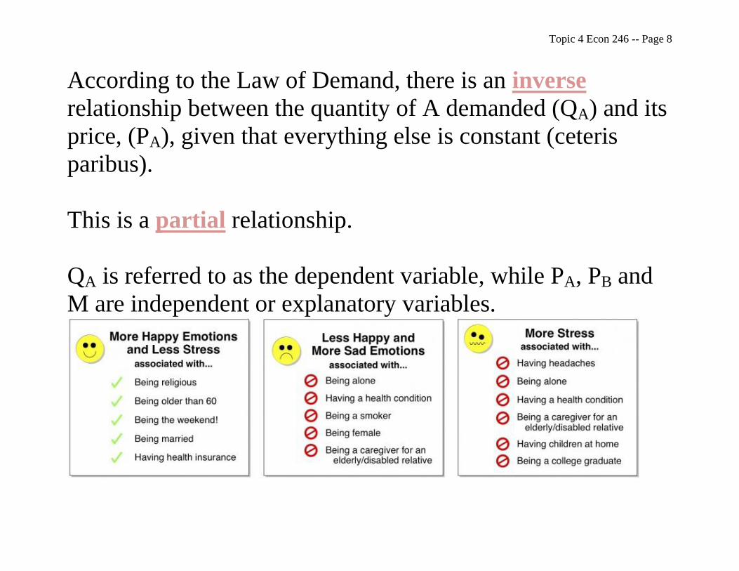
According to the Law of Demand, there is an inverse

relationship between the quantity of A demanded (QA) and its

price, (PA), given that everything else is constant (ceteris

paribus).

This is a partial relationship.

QA is referred to as the dependent variable, while PA, PB and

M are independent or explanatory variables.

Topic 4 Econ 246 --

Economic theory dictates the variable or variables

whose values determine the behaviour of a variable of

interest.

i.e. Economic theory make claims about the variables the

affect the value of the variable of interest.

For example, the price of a new car will determine the

quantity of cars demanded.

Or the interest rate on mortgages, CPI and the GDP may

partially determine the demand for new housing.

Topic 4 Econ 246 --

But:

(i) Economic theory does not always provide the expected

signs for all explanatory variables.

Example: PB: its sign is the demand function depends on

whether the good is a complement or substitute good.

(ii) Economic theory does not always provide clear and

precise information about the functional form of the

function.

The functional form of these type of relationships must

be specified before estimation can take place.

Otherwise, estimation of economic theory can be

misleading.

Topic 4 Econ 246 --

Example: A linear demand function is specified

QA=β1+β2PA+β3PB+β4M

Where the βi’s are the parameter of the model.

Parameters are usually unknown.

We often wish to estimate them.

Note: QA, PA, PB, and M may be transformations of non-linear

data:

For example: C

AQ

Q1

or .2

AC QQ

Topic 4 Econ 246 --

These non-linear relationships have been transformed

into a linear format and hence, expressed in a linear

regression model.

For example:

Sales

Sales

SalesSales

QQ

QQ

1

2

Once we have determined the functional form of the

regression, we can address questions such as:

If we change the income tax laws, will there be an effect

on the quantity of new homes demanded, which works

through disposable income?

Topic 4 Econ 246 --

Are goods A and B substitutes or complements (which is

determined by cross price elasticities)? If the price of B

rises, does the quantity of A increase or decrease?

If PB increases and it is a complement: QA demanded

decreases.

Example: Quantity of large vehicles demanded decreases

when the price of gasoline increases.

Example: the price of batteries and the demand for battery

powered toys.

If PB increases and it is a substitute: QA demanded

increases.

Topic 4 Econ 246 --

Example: Quantity of apples demanded increases when the

price of oranges increases.

Apples and oranges are substitutes.

Above we had examples of exact relationships between

the dependent variable and the explanatory variables.

The functional relationships were deterministic ( i.e. no

uncertainty involved.)

However, in the real world, such relationships are not as

simple or straight forward.

Topic 4 Econ 246 --

For illustration, if we look at two businesses that build

the same product, and face the same production costs

and factor prices, their demands are not usually the

same.

There are many other individual factors that have been

ignored. (Firm’s ideology, skill level of employees,

marketing experience, etc.)

There will be some uncertainty: “stochastic” function.

Example: Suppose we have several households with the same

income, facing the same prices. The typical demands

from each household will differ because other

individual factors have been ignored by the model.

Topic 4 Econ 246 --

Such as: tastes

Beliefs

Health

Influence of advertising

Age

Gender

These factors project uncertainty into the function.

This stochastic element is incorporated into the

function by including a “stochastic” error term into the

model.

MPPQ XYY 4321

Topic 4 Econ 246 --

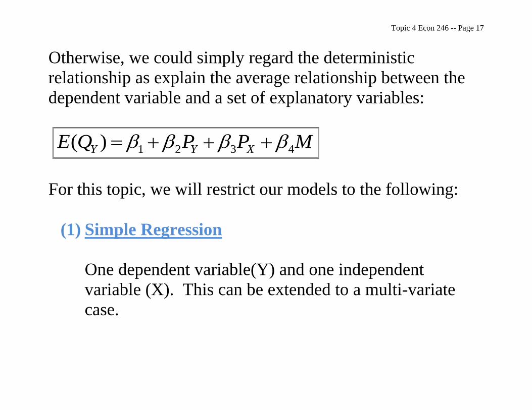
Otherwise, we could simply regard the deterministic

relationship as explain the average relationship between the

dependent variable and a set of explanatory variables:

MPPQE XYY 4321)(

For this topic, we will restrict our models to the following:

(1) Simple Regression

One dependent variable(Y) and one independent

variable (X). This can be extended to a multi-variate

case.

Topic 4 Econ 246 --

(2) Linear Parameters:

We assume the relationship between the dependent variable

and the independent variable is linear in terms of parameters:

XYE )(

Population regression line is linear in terms of parameters α

and β, which depict the functional relationship between X and

Y.

(3) XYE )( Means for a given value of X, the

expected value of Y (average) is given by X .

Topic 4 Econ 246 --

We expect Y, [E(Y)], to change as X changes.

Use subscripts to denote which observation of X and Y

we are looking at: ii XYE )( for observation i.

Parameters:

α is referred to as the (population) Y-intercept term

β denotes the (population) slope term which is the

derivative of Y with respect to X:

x

y.

Topic 4 Econ 246 --

Yi

(Xi,Yi)

* ii XYE )(

* ε * * *

*

Slope = β E(Yi)

*

α *

X

Xi

Topic 4 Econ 246 --

Example: Let Y be the crime rate and X represent the

unemployment rate. Then for the ith

observation, the expected

value of crime is:

E(crime) = α + β(Unemployment rate) for the ith

observation.

E(Yi) = α + β (Xi) for the ith

observation.

For each city with the same X (unemployment rate) actual

crime (Y) varies because of the “other” factors involved.

For observation i:

ii XY Population regression model

Topic 4 Econ 246 --

where )( ii YEY

which represents the difference between the actual observed

Yi (crime rate) and the population regression line, E(Yi).

β – the slope – measures the marginal product of a change in

the unemployment rate which is implicit in a change in the

crime rate.

Another Example:

Let Yi be the number of years of post secondary education

for individual i.

Topic 4 Econ 246 --

Le Xi be the number of years of post secondary education by

one of the parents (either by the father or mother, whoever

has more education,) of individual i.

Suppose we know that α = 1.3 and β= 0.8. Then the

population regression line is:

ii XY 8.03.1

Or

ii XYE 8.03.1)(

Topic 4 Econ 246 --

Notes on this example:

(i) Suppose the individual ‘i’ is Jason. One of his parents

has four years of post secondary schooling. How

many years of post secondary education do we

expect Jason to have, ceteris paribus?

Xi =4, so:

yearsYE

YE

XYE

i

i

ii

5.4)(

)4(8.03.1)(

8.03.1)(

On average, we expect an individual with a parent that has 4

years of post secondary schooling to complete 4.5 years of

post secondary schooling.

Topic 4 Econ 246 --

(ii) Other factors affect Yi for i= Jason.

If the number of years of schooling is in fact 4.5, the random

error term, εi, equals zero: εi=0.

But, if the actual number of years of school competed is

seven years, εi=2.5 for Jason.

Obviously, regression analysis is useful since it allows us to

quantify the association or relationship among variables.

We can determine how variable affect each other

numerically!

Topic 4 Econ 246 --

Individual’s Schooling (Yi)

7 ii XYE 8.03.1)(

εi=2.5

4.5

5.4)( iYE 1.3

Parent’s schooling 0 4 Xi

Topic 4 Econ 246 --

The Sample Regression Model

(α and β Unknown)

In the previous examples, we assumed that we knew the value

of α and β – the population parameters.

This is unrealistic, and we usually must estimate α and β

using sample data.

I.e. this is analogous to using X as an estimator of µ, or s2 as

an estimator of σ2.

Topic 4 Econ 246 --

Questions:

1) How do we decide which estimators to use for estimating

α and β?

2) How can we use sample information?

Topic 4 Econ 246 --

The sample regression line takes the form:

ii bXaY ˆ

Where:

(i) The “hat” indicates a “fitted value” or a calculated

value.

(ii) ‘a’ is the estimator of α.

(iii) ‘b’ is the estimator of β.

(iv) The ‘i’ subscript indicate the ith

observation and

includes all observations in the sample from 1 to n

(n=sample size.)

Topic 4 Econ 246 --

As with the population regression line, ii YY ˆ, typically.

The difference between ii YandY , the sample error, is

denoted ei: iii YYe ˆ

Substituting:

iiiii bXaYebXaY ˆ

Hence, we can express the sample regression model as:

iii ebXaY

Topic 4 Econ 246 --

Note:

ei is the sample error.

εi is the population error.

They are not the same thing.

ei is observable.

εi is not observable.

.

.,

parameterspopulationunknownareandXY

andofestimatessampleknownarebabXaYe

iii

iii

Topic 4 Econ 246 --

In general, banda . }

The usual distinction between a sample and a population.

Let ei (the sample error) be referred to as the residual term.

Let εi (the population error) be referred to as the disturbance

term.

Let ‘a’ be our estimator of α derived from a sample.

Let ‘b’ be our estimator of β derived from a sample.

Since an estimator is a formula or rule, we must determine ‘a’ and ‘b’ from the sample information.

Which method should be employed, since there are many

possible estimators?

Topic 4 Econ 246 --

The Method of Least Squares

Recall we have restricted our discussion in this topic to a two-

variable (bivariate) model which is linear in parameters.

ii XY

This model is linear in variables (Y and X) as well as

parameters.

But, it is not necessary to restrict our variables this way.

Topic 4 Econ 246 --

Topic 4 Econ 246 --

Example:

Regression analysis can handle:

(i) Log-linear models: ii XYLog )(

or

(ii) Log-Log models: )()( ii XLOGYLog

These models are linear in parameters, but non-linear in

variables.

By redefining the variables: )log(

)log(

*

*

ii

ii

xX

YY

, the models are

linear in the new variables:

Topic 4 Econ 246 --

iii XYYLog *)( and

**

)()(

ii

ii

XY

XLOGYLog

respectively.

What is important for the following analysis is that our

parameters are linear.

Topic 4 Econ 246 --

Least Squares:

Suppose we have a sample of size n, with (Xi,Yi) pair value.

Plot the data points with the Yi’s on the vertical axis and Xi’s

on the horizontal axis.

Yi *

*

* *

*

* *

*

*

0 Xi

Topic 4 Econ 246 --

We can derive a fitted line that passes through these values by

measuring α and β by values a and b, such that the fitted line

passes close to the observed data.

Yi

ii bXaY ˆ

*

* *

*

* *

*

*

0 Xi

Topic 4 Econ 246 --

How should we choose a and b?

By minimizing the distance between the actual observation

and the fitted line:

To illustrate, isolate one point:

Yi

ii bXaY ˆ

*

* *

ei *

* *

* iY

* Yi

0 Xi

Topic 4 Econ 246 --

We want the sum of the residuals to be small as possible.

The problem with choosing a and b so as to minimize

n

i

ie1

, is

offsetting signs.

We could:

(i) Minimize

n

i

ie1

Or

(ii) Minimize ApproachSquaresLeasten

i

i 1

2

Topic 4 Econ 246 --

Why Use The Least Squares Approach?

(I) All observations are given equal weight.

(II) Our estimators of α and β, a and b respectively, have

good statistical properties:

(i) Unbiased: E(a)= α and E(b)= β.

(ii) Efficient: minimum variance estimators out of

all linear unbiased estimators (BEST)

(III) Computationally simple (closed form analytic solution

to minimization problem.)

(IV) Extends trivially to multivariate and non-linear

relationships.

Topic 4 Econ 246 --

Thus, least squares (LS) estimators of α and β are those

estimators of a and b which minimize the sum of the squared

residuals.

Mathematically, least squares problem is:

n

i

ii

n

i

ii

n

i

i

ii

n

i

ii

n

i

iba

bXaYYYeG

Gs

bXaYwhere

YYeGMin

1

2

1

2

1

2

1

2

1

2

),(

ˆ

:intoexpressionabovethengsubstitutio

ˆ

ˆ

Solve this minimization problem using calculus.

Topic 4 Econ 246 --

Partially differentiate G with respect to a and b and equate

these firsts order conditions (FOC) to zero. This results in

two equations with two unknowns and we solve for a and b.

n

i

n

i

iii

n

i

ii

n

i

ii

n

i

ii

n

i

ii

n

i

iba

ebXaY

bXaY

FOCbXaYa

bXaY

a

Gi

bXaYeGMin

1 1

1

11

2

1

2

1

2

),(

00 :equation normal theyieldswhich

02

)(0)1(2)(

Taking the summation sign through:

Topic 4 Econ 246 --

...

11

:nby dividing

:

0

0

11

11

11

111

ofestimatorSLXbYa

Xn

bYn

a

XbYna

grearrangin

XbnaY

bXaY

n

i

i

n

i

i

n

i

i

n

i

i

n

i

i

n

i

i

n

i

i

n

i

n

i

i

Topic 4 Econ 246 --

0

(*) into that substitute we,Since

(*)0

0

0 :equation normal theyieldswhich

02

)(0)(2)(

1

2

1

1

2

1

1

2

11

1

2

1

2

11

2

n

i

i

n

i

ii

n

i

i

n

i

ii

n

i

i

n

i

i

n

i

ii

n

i

iiii

n

i

iiii

n

i

ii

n

i

ii

XbXnXbYYX

XbYa

XbXanYX

XbXaYX

bXaXYX

bXaXYX

FOCXbXaYb

bXaY

b

Gii

Topic 4 Econ 246 --

.

)(

:LHS on the is b""such that gRearrangin

0)(

0

0

1

22

1

11

22

1

22

1

1

22

1

1

2

1

ofEstimatorSquaresLeast

XnX

YXnYX

b

YXnYXXnXb

XXnbYXnYX

XbXnbYXnYX

XbXnXbYYX

n

i

i

n

i

ii

n

i

ii

n

i

i

n

i

i

n

i

ii

n

i

i

n

i

ii

n

i

i

n

i

ii

Topic 4 Econ 246 --

So, the least squares formulae for a and b for fitting our linear

regression model to the data are:

XbYa

.

1

22

1

n

i

i

n

i

ii

XnX

YXnYX

b

Topic 4 Econ 246 --

Can also write b as:

n

i

i

n

i

ii

n

i

i

n

i

ii

XXn

YYXXn

b

or

XX

YYXX

b

1

2

1

1

2

1

)()1(

1

))(()1(

1

)(

))((

Topic 4 Econ 246 --

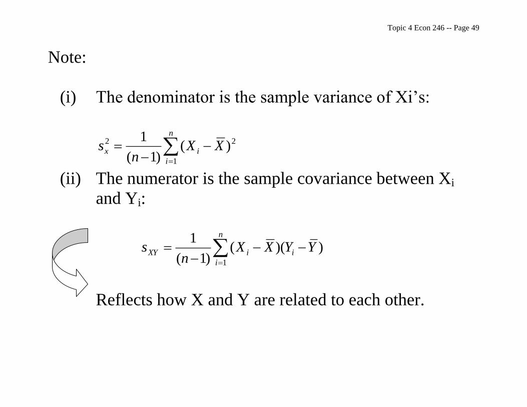
Note:

(i) The denominator is the sample variance of Xi’s:

n

i

ix XXn

s1

22 )()1(

1

(ii) The numerator is the sample covariance between Xi

and Yi:

))(()1(

1

1

YYXXn

sn

i

iiXY

Reflects how X and Y are related to each other.

Topic 4 Econ 246 --

Thus, we can also write:

variableindep. of varianceSample

variabledep. & indep.between COV Sample2

X

XY

S

Sb

Topic 4 Econ 246 --

(iii) The sample regression line always passes through the

point: ( YX , ).

Recall, the fitted regression model is:

Y a bX a bX

but,

a Y bX

so,

Y Y bX bX Y

when

X X.

i i

i

i

The sample regression line always passes through the

point YX , .

Topic 4 Econ 246 --

Yi

ii bXaY ˆ

*

* *

Y *

* *

*

*

0 Xi

X

Topic 4 Econ 246 --

(iv) With the least squares procedure, the sum of the errors

(residuals) equals zero:

n

i

ii

n

i

i bXaYe11

0

Recall the normal equation for determining a:

Topic 4 Econ 246 --

n

i

ii

n

i

n

i

iii

n

i

i

n

i

n

i

i

n

i

i

n

i

i

YY

ebXaY

XbaY

zerotoEquate

XbnaY

1

1 1

111

11

0)ˆ(

00

0

:

The sum of the least squares residuals is always zero.

Topic 4 Econ 246 --

The least squares line is derived such that the line will

be situated amongst the data values such that the

positive residuals (under-estimates of actual points)

always exactly cancel out the negative residuals (over-

estimates of actual points).

Example: Gas prices (X) and Bike sales (Y)

Sales of Bikes (Y)

(millions)

Gas prices (X)

6 0.75

6.5 0.85

8 0.95

10.3 1.05

12 1.15

9 1.25

Topic 4 Econ 246 --

Sample size, n=6.

Estimate the population intercept and slope by least

squares estimators a and b to determine the sample

regression model. ii bXaY ˆ

Sales of Bikes

(Y) (millions)

Gas prices

(X)

($/litre)

2

iX XiYi

6 0.75 0.5625 4.5

6.5 0.85 0.7225 5.525

8 0.95 0.9025 7.6

10.3 1.05 1.1025 10.815

12 1.15 1.3225 13.8

9 1.25 1.5625 11.25

iY =51.8 iX =6 2

iX =6.175 iiYX =53.49

Topic 4 Econ 246 --

49.53

175.6

16/6

633.86/8.51

2

ii

i

YX

X

X

Y

669.9

175.0

692.1

175.0

798.5149.53

)1)(6(175.6

)633.8)(1)(6(49.532

1

22

1

n

i

i

n

i

ii

XnX

YXnYX

b

0356.1)1)(669.9(633.8 XbYa

ii XY 669.90356.1ˆ

For each $1 increase in the price of gas, bike sales will

increase by 9.7 million.

Topic 4 Econ 246 --

If you put a “hat” on the dependent variable, iY , then

you do not have to put the residual(ei) into the

regression line. If you do not put the “hat” on the Yi

then you must include the ei.

Forecasting:

If price is $1.50, then:

4679.13)50.1(669.90356.1ˆ

669.90356.1ˆ

i

ii

Y

XY

The best estimate of bike sales is 13.5 million.

Topic 4 Econ 246 --

Topic 4 Econ 246 --

Summary: Regression Model -- Terms and Symbols

Term Population Symbol Sample Symbol

Model ii XY iii ebXaY

Error εi ei

Slope β b

Intercept α a Equation of

the line: ii XYE )( ii bXaY ˆ

Topic 4 Econ 246 --

Concluding Remarks:

1) The least squares procedure is simply a curve-fitting

technique. It makes no assumptions about the

independent variable(s), X, the dependent variable, Y, or

the error term.

2) We will need to make assumptions about the independent

variables, the dependent variable and the error term if we

wish to consider how well ‘a’ and ‘b’ estimate α and β.

3) We will also need to make assumptions if we want to form

interval estimates for predicted values of Y or interval

estimates for α and β. (Impose some restrictions on how

X behaves, or distributed.)

Topic 4 Econ 246 --

4) We will need assumptions if we want to test any

hypotheses about the population parameters.

Example: 0

00

:

:

aH

H

, where β0 is some known

value.

Special test: 0:

0:0

aH

H

. This tests to see if X is

significant in explaining Y.

5) We can extend least squares principle to non-linear

models.

Topic 4 Econ 246 --

6) We use least squares because it can be shown that under

certain assumptions, a and b are unbiased estimators of α

and β, respectively. They are also consistent and efficient

(i.e. minimum variance).

In other words, under certain assumptions, a and b are the

best unbiased estimators of α and β, respectively.

Topic 4 Econ 246 --

Assumptions and Estimator Properties

The population model is: ii XY ,

where i=1, 2, 3…N.

The Five Assumptions:

Gauss-Markov Theorem: Given the five basic assumptions,

(below,) the least squares estimators in the linear

regression model ae best linear unbiased

estimators: “BLUE”

Topic 4 Econ 246 --

Assumption #1:

The random variable ε is statistically independent of X.

That is, E(ε,X)=0.

Always holds if X is non-stochastic (fixed in

repeated sampling.)

Assumption #2:

εi is normally distributed for all i.

Assumption #3:

E(ε )=0. That is, on average the disturbance term is

zero for all i.

Topic 4 Econ 246 --

Assumption #4:

Var(εi)= .2

iXandi

This is known as the assumption of

homoscedasticity or constant variance, across all

observations. Otherwise, heteroscedastic.

Assumption #5:

Any two errors εi and εj are statistically

independent of each other for i≠j. That is, zero

covariance (disturbances ae uncorrelated). For

example, disturbance in observation 1 does not

affect observation 2, etc.

Topic 4 Econ 246 --

If disturbances are correlated across observations, then there

exists autocorrelation or serial correlation.

Topic 4 Econ 246 --

Remarks:

1) From assumptions 1 through 4, we have .),0(~ 2 iNi

2) Yi is random only because εi is random if X is non-

random or non-stochastic.

3) iiii XXEYE )()(

Since Xi is non-stochastic and E(εi)=0.

2)()()( iiii VarXVarYVar .

Since α, β, and X are non-stochastic (No variability).

Yi is a linear function of εi and is normal.

That is, from ,),0(~ 2

Ni it follows that ).,(~ 2

ii XNY

Topic 4 Econ 246 --

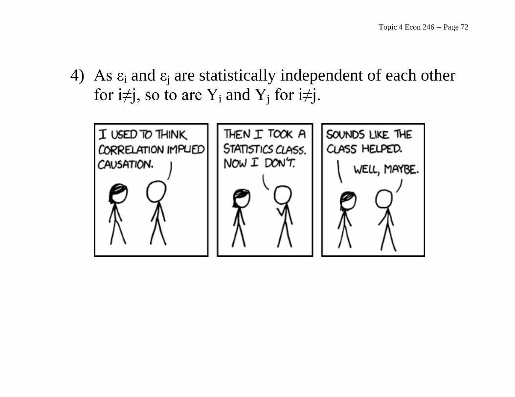
4) As εi and εj are statistically independent of each other

for i≠j, so to are Yi and Yj for i≠j.

Topic 4 Econ 246 --

Measures of Goodness of Fit

This section will explore two measures of goodness of fit:

1) The standard error of the estimate: which is the

measure of the absolute fit of the sample points to

the sample regression line.

2) The coefficient of determination R2: which is a

measure of the relative goodness of fit of a sample

regression line.

Topic 4 Econ 246 --

Notation:

Total deviation of Y: the difference between the observed

value of Yi and the mean of the Y-values, Y .

YYi (By adding and subtracting Y , we can separate the

deviation into two parts:)

The total deviation can be expressed as the sum of two other

deviations:

ii YY ˆ and YYi ˆ

.

The first deviation expression is the residual ei: iii eYY ˆ

.

Topic 4 Econ 246 --

Since the ei’s are random, the term iii eYY ˆ is referred

to as the unexplained deviation.

(We cannot determine why ii YY ˆ ).

The second deviation can be explained by the regression line.

YYi ˆ

is the explained deviation, because it is possible to

explain iY differs from Y because Xi differs from

X .

Total Deviation = Unexplained Deviation+ Explained Deviation

YYi = ii YY ˆ + YYi ˆ

Topic 4 Econ 246 --

Y

Regression line

Y Explained

iY Unexplained

Yi

X

Topic 4 Econ 246 --

Y

Yi Regression line

Unexplained dev.

iY

Explained dev.

Y

X

Topic 4 Econ 246 --

The two parts of the total deviation are independent.

Hence, we can square each deviation and sum over all ‘n’

observations as follows:

2

1

2

1

2

1

ˆˆ

n

i

i

n

i

i

n

i

i YYYYYY

Breaking into three parts:

Topic 4 Econ 246 --

SST

squares of sum totalThe

variation totalThe

2

1

n

i

i YY

n

i

n

i

i YY

1

2

i

2

1

eSSE

error squares of sum The

variationdunexplaine Theˆ

Topic 4 Econ 246 --

SSR

regression squares of sum The

.regression e th

todue variationexplained Theˆ2

1

n

i

i YY

SSR SSE SST

ˆˆ

deviation Explained deviation dUnexplainedeviation Total

2

1

2

1

2

1

n

i

i

n

i

i

n

i

i YYYYYY

Topic 4 Econ 246 --

Why are we dissecting the total variation

into two components?

We can now determine the goodness of fit of a regression in

terms of the size of SSE.

If the fit is perfect, SSE = 0. iYY ii ˆ

If the fit is not perfect SSE≠0

Topic 4 Econ 246 --

Calculation of SST, SSR and SSE

The best way to illustrate the calculation of these measures is

through the example from earlier:

Sales of Bikes

(Y) (millions)

Gas prices

(X)

($/litre)

2

iX XiYi

6 0.75 0.5625 4.5

6.5 0.85 0.7225 5.525

8 0.95 0.9025 7.6

10.3 1.05 1.1025 10.815

12 1.15 1.3225 13.8

9 1.25 1.5625 11.25

iY =51.8 iX =6 2

iX =6.175 iiYX =53.49

Topic 4 Econ 246 --

49.53

175.6

16/6

633.86/8.51

2

ii

i

YX

X

X

Y

669.9

175.0

692.1

175.0

798.5149.53

)1)(6(175.6

)633.8)(1)(6(49.532

1

22

1

n

i

i

n

i

ii

XnX

YXnYX

b

0356.1)1)(669.9(633.8 XbYa

ii XY 669.90356.1ˆ

Topic 4 Econ 246 --

Sales of

Bikes (Y)

(millions)

Gas prices

(X)

($/litre)

2YYi Total deviation

22 ˆiii YYe

Unexplained

deviation

2ˆ YYi

Explained

deviation

iY

6 0.75 6.932689 0.046720823 5.841163922 6.21615

6.5 0.85 4.549689 0.466557303 2.102355003 7.18305

8 0.95 0.400689 0.022485002 0.233337303 8.14995

10.3 1.05 2.778889 1.399843923 0.234110823 9.11685

12 1.15 11.336689 3.672014063 2.104675563 10.08375

9 1.25 0.134689 4.205165423 5.845031523 11.05065

iY =51.8 iX =6 SST=26.1333 SSE=9.81279 SSR=16.3607

We should find that SST=SSR+SSE

A more convenient way to determine SST is the

following:

2

11

2 1

n

i

i

n

i

i Yn

YSST

Topic 4 Econ 246 --

The amount of variation explained by the regression

equation can be determined without first calculation SSE.

The method eliminates the calculation of each estimated

value ( iY ).

Explained variation:

Y) and X ofion b(covariat

))((

YYXXbSSR ii

Once SST and SSR are found, the unexplained variation,

SSE, is found by subtraction:

SSE=SST-SSR.

Topic 4 Econ 246 --

How Good is the Fit In Regression Analysis?

(I) Standard Error of the Estimate

2

ˆ2

1

1

2

n

SSEYY

nS

n

i

iie

The number of degrees of freedom in this case is n-2 because

two sample statistics (a and b) must be calculated

before the value of iY can be computed.

The information from this statistic provides an indication of

the fit of the regression model. It also indicates the

size of the residuals that result.

Topic 4 Econ 246 --

The units of Se are always the same as those for the variable

Y since ‘e’ is a leftover (residual) component of Y.

Problem: (units) Is Se large or small?

To determine whether Se is large of small, we compare it to

the average size of Y.

Using a coefficient of variation type measure, we can define

the typical percentage error in predicting Y using the

sample data and the regression line.

Topic 4 Econ 246 --

Coefficient of Variation For the Regression Residuals:

First compute the Se:

5663.1453197.226

81279.9

2ˆ

2

1

1

2

n

SSEYY

nS

n

i

iie

1429.18100633.8

5663.1100:..

Y

SresidualsVC e

For this example, the C.V. residuals = 18.14%. In predicting

the number of bike sales, the value will be incorrect by

18.14% on the average.

Topic 4 Econ 246 --

(II) Coefficient of Determination

The second measure of goodness of fit is the

coefficient of determination. (R2)

It facilitates in the interpretation of the relative amount

of variation that has been explained by the sample

regression line.

Topic 4 Econ 246 --

Deriving R2:

Recall: SST=SSE+SSR

If we divide this expression by SST: SST

SSR

SST

SSE

SST

SSR

SST

SSE

SST

SST

1 .

These two ratios must sum to one and are mutually exclusive.

Recall, SSE is the unexplained variation in Y.

Topic 4 Econ 246 --

The ratio SST

SSE

represents the proportion of total variation that

is unexplained by the regression relation.

The ratio SST

SSR

represents the relative measure of goodness of

fit and is called the coefficient of determination.

It measures the proportion of total variation that is explained

by the regression line.

. variationTotal

explainedVariation 2 SST

SSRR

Topic 4 Econ 246 --

If the regression line perfectly fits all the sample points,

SSR=SST and the coefficient of determination would

achieve its maximum value of 1: R2=1.

Y

Regression line

*

*

*

*

X

Perfect fit: R2 =1; ii YY ˆ

Topic 4 Econ 246 --

As the degree of fit becomes less accurate and less of the

variation in Y is explained by their relation with X, R2

decreases.

Y

* Regression line

*

* * * *

* *

*

X

{0<R2<1}

Topic 4 Econ 246 --

The lowest value of R2 is zero, which will occur whenever SSR=0

and SSE=SST. This occurs when YYi ˆ

for all

observations.

Y

* *

* *

* * * * Regression line

* * * *

* * * *

X There is no systematic relation between Y and X:

R2=0; YYi

ˆ ; b=0.

The regression line is horizontal with a slope =0.

Hence, X has no effect in explaining Y.

Topic 4 Econ 246 --

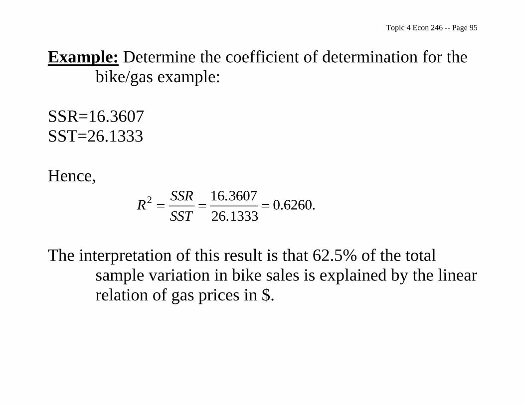
Example: Determine the coefficient of determination for the

bike/gas example:

SSR=16.3607

SST=26.1333

Hence,

.6260.0

26.1333

16.36072 SST

SSRR

The interpretation of this result is that 62.5% of the total

sample variation in bike sales is explained by the linear

relation of gas prices in $.

Topic 4 Econ 246 --

The remaining 37.4% of the variation in bike sales is still

unexplained.

Most likely some other variable has been omitted from the

regression model that could explain some additional

portion of the variation. (“Multiple regression model”

is required.)

Topic 4 Econ 246 --

Topic 4 Econ 246 --

Correlation Analysis

The measurement of how well two or more variables vary

together is called correlation analysis.

One measure of the population relationship between two

random variables is the population covariance:

)])([(),( YYXXEYXCov ii

Usually this measure is not a good indicator of the relative

strength of the relationship between two variables

because its magnitude depends on the units used to

measure the variables.

Topic 4 Econ 246 --

Hence, it is necessary to standardize the covariance of two

variables in order to have a good measure of fit. (Unit-

less measure.)

Standardization is carried out by dividing the covariance of X

and Y by the standard deviation of X times the

standard deviation of Y:

This is referred to as:

YX

YXCov

),(

Y) of dev. (STD.X) of dev. (STD.

Y and X of Covariance

:tCoefficienn Correlatio Population

Topic 4 Econ 246 --

Three Special Cases:

Case #1: Perfect Positive Correlation: ρ= 1.

All values of X and Y fall on a positively sloped straight line:

Topic 4 Econ 246 --

Case #2: Perfect Negative Correlation: ρ = -1.

All values of X and Y fall on a negatively sloped straight line.

Topic 4 Econ 246 --

Case #3: Zero Correlation: ρ=0.

If X and Y are not linearly related, they are independent

random variables. Then, the value of the correlation

coefficient will be zero, since Cov(X,Y)=0.

Topic 4 Econ 246 --

Thus, ρ measures the strength of the linear association

between X and Y.

Values of ρ close to zero indicate a weak relation;

Values close to +1 indicate a strong positive relation;

Values close to -1 indicate a strong negative correlation.

Sample Correlation Coefficient

We employ sample data to estimate the population parameter

ρ. The sample correlation coefficient is denoted by the

letter ‘r’.

We determine the value of ‘r’ in the same manner as ρ, except

that we substitute for each population parameter its

best estimate based on the sample data.

Topic 4 Econ 246 --

n

i

iiXY

XY

YYXXn

S

S

1

))((1

1

::Covariance Sample

The Sample Correlation Coefficient:

Variations Sample

ncovariatio Sample

:freedom of degrees out the divide

)(1

1)(

1

1

))((1

1

Y ofdeviation

standard Sample

X ofdeviation

standard Sample

Y and X of valuessample Cov.

1

2

1

2

1

YX

XY

n

i

i

n

i

i

n

i

ii

YX

XY

SSSS

SCr

YYn

XXn

YYXXn

SS

Sr

Topic 4 Econ 246 --

The Connection Between Correlation and Regression

1) The correlation coefficient and the coefficient of

determination measure the strength of the association

between X and Y.

For a model with only one explanatory variable, the

measure of R2 is the square of the correlation measure

‘r’, as they measure the same relationship.

When there is a weak relationship, both measures are

close to zero.

Topic 4 Econ 246 --

A strong relation is indicated between the two variables,

X and Y, when r approaches -1 or +1.

And, since the square of ‘r’ is always positive, R2

approaches +1 when there is a strong relation.

Topic 4 Econ 246 --

2) The correlation coefficient provides information about

the direction of the association between X and Y.

Either positively or negatively related.

A positive correlation must always correspond to a

regression line with a positive slope (b), indicating a

direct relationship.

A negative correlation corresponds to an inverse

relationship.

Topic 4 Econ 246 --

3) In correlation analysis the X and Y variables are

assumed to have probability distribution.

In regression analysis, the independent variable X can be

considered as a set of given values.

When X is an independent random variable, correlation

between X and Y is zero.

Topic 4 Econ 246 --

Topic 4 Econ 246 --

4) In correlation analysis there is no specified “dependent”

and “independent” variable designation.

In regression analysis we impose a model, such that Y is

being explained by X.

If the dependent and independent variables are switched, the

regression model will not be the same, although the sign on the

slope parameter will remain the same.

Topic 4 Econ 246 --

topic 4: simple correlation and regression analysisweb.uvic.ca/~bettyj/246/topic4new.pdf · topic 4...

Documents