topic 3 drawing inferences · topic 3: drawing inferences in this topic, students continue...

Lesson 1We Want to Hear From You!Collecting Random Samples . . . . . . . . . . . . . . . . . . . . . . . . . . . . . . . . . . . . . . . . M4-133

Lesson 2Tiles, Gumballs, and PumpkinsUsing Random Samples to Draw Inferences . . . . . . . . . . . . . . . . . . . . . . . . . . . . M4-151

Lesson 3Spicy or Dark?Comparing Two Populations . . . . . . . . . . . . . . . . . . . . . . . . . . . . . . . . . . . . . . . . M4-169

Lesson 4Finding Your Spot to LiveUsing Random Samples from Two Populations to Draw Conclusions . . . . . . . . . M4-181

Choosing a sample randomly from a population is a good way to select items that are representative of the entire population.

TOPIC 3

Drawing Inferences

C02_SE_M04_T03_INTRO.indd 129C02_SE_M04_T03_INTRO.indd 129 1/14/19 11:44 AM1/14/19 11:44 AM

C02_SE_M04_T03_INTRO.indd 130C02_SE_M04_T03_INTRO.indd 130 1/14/19 11:44 AM1/14/19 11:44 AM

Carnegie Learning Family Guide Course 2

Module 4: Analyzing Populations and ProbabilitiesTOPIC 3: DRAWING INFERENCESIn this topic, students continue developing their understanding of the statistical process by focusing on the second component of the process: data collection. They learn about samples, populations, censuses, parameters, and statistics. Students display data and compare the difference of the measures of center for two populations to their measures of variation. Then students draw conclusions about two populations using random samples.

Where have we been?In grade 6, students learned about and used aspects of the statistical problem-solving process: formulating questions, collecting data, analyzing data, and interpreting the results. They also used numerical data displays, including both measures of center (mean, median, mode) and measures of variation (mean absolute deviation, range, and interquartile range).

Where are we going?In high school, students will learn about specifi c types of random sampling and the inherent bias in sampling techniques. They will continue analyzing and comparing random samples from populations and comparing their measures of center and variation.

Using a Random Number Table to Select Random Samples

When selecting samples for an experiment, a random number table can be used to assign individuals to groups. The fi rst three lines of a sample random number table are shown.

TOPIC 3: Family Guide • M4-131

Random Number Table

Line 1 65285 97198 12138 53010 94601 15838 16805 61404 43516 17020

Line 2 17264 57327 38224 29301 18164 38109 34976 65692 98566 29550

Line 3 95639 99754 31199 92558 68368 04985 51092 37780 40261 14479

C02_SE_FG_M04_T3.indd 131C02_SE_FG_M04_T3.indd 131 1/14/19 11:11 AM1/14/19 11:11 AM

Myth: Faster = smarter.In most cases, speed has nothing to do with how smart you are. Why is that? Because it largely depends on how familiar you are with a topic. For example, a bike mechanic can look at a bike for about 8 seconds and tell you details about the bike that you probably didn’t even notice (e.g., the front tire is on backwards). Is that person smart? Sure! Suppose, instead, you show the same bike mechanic a car. Will s/he be able to recall the same amount of detail as for the bike? No!

It’s easy to confuse speed with understanding. Speed is associated with the memorization of facts. Understanding, on the other hand, is a methodical, time-consuming process. Understanding is the result of asking lots of questions and seeing connections between different ideas. Many mathematicians who won the Fields Medal (i.e., the Nobel prize for mathematics) describe themselves as extremely slow thinkers. That’s because mathematical thinking requires understanding over memorization.

#mathmythbusted

M4-132 • TOPIC 3: Drawing Inferences

Talking Points You can support your student’s learning by approaching problems slowly. Students may observe a classmate learning things very quickly, and they can easily come to believe that mathematics is about getting the right answer as quickly as possible. When this doesn’t happen for them, future encounters with math can raise anxiety, making problem solving more diffi cult, and reinforcing a student’s view of himself or herself as “not good at math.” Slowing down is not the ultimate cure for math diffi culties. But it’s a good fi rst step for children who are struggling. You can reinforce the view that learning with understanding takes time, and that slow, deliberate work is the rule, not the exception.

Key Termsparameter

When data are gathered from a population, the characteristic used to describe the population is called a parameter.

statistic

When data are gathered from a sample, the characteristic used to describe the sample is called a statistic.

random sample

A random sample is a sample that is selected from the population in such a way that every member of the population has the same chance of being selected.

C02_SE_FG_M04_T3.indd 132C02_SE_FG_M04_T3.indd 132 1/14/19 11:11 AM1/14/19 11:11 AM

LESSON 1: We Want to Hear From You! • M4-133

1

LEARNING GOALS• Differentiate between a population and a sample. • Differentiate between a parameter and a statistic.• Differentiate between a random sample and a

non-random sample.• Identify the benefits of random sampling of a

population, including supporting valid statistical inferences and generalizations.

• Use several methods to select a random sample.

KEY TERMS• survey • data • population • census

• sample • parameter • statistic• random sample

WARM UPLight It Up Light Bulb Company tests 24 of the bulbs they just produced and found that 3 of them were defective. Use proportions to predict how many light bulbs would be defective in shipments of each size.

1. 100 light bulbs

2. 400 light bulbs

3. 750 light bulbs

We Want to Hear From You!Collecting Random Samples

The statistical process is a structure for answering questions about real-world phenomena. How can you make sure that the data you collect accurately answer your statistical questions?

C02_SE_M04_T03_L01.indd 133C02_SE_M04_T03_L01.indd 133 1/14/19 9:51 AM1/14/19 9:51 AM


Getting Started

Reviewing the Statistical Process

There are four components of the statistical process:

• Formulating a statistical question.• Collecting appropriate data.• Analyzing the data graphically and numerically.• Interpreting the results of the analysis.

1. Summarize each of the four components. You may want to use examples to support your answers.

How could you describe the students in your classroom? How do the students in your classroom compare to other groups of students in your school, or to other seventh graders in the United States?

2. Formulate a statistical question about your classmates. How might you collect the information to answer your question?

One data collection strategy you can use is a survey. A survey is a method of collecting information about a certain group of people. It involves asking a question or a set of questions to those people. When information is collected, the facts or numbers gathered are called data.

3. Answer each question in the survey shown. You will use the results in the next activity.

a. What is your approximate height?

b. Do you have a cell phone? Yes No

c. About how many text messages do you send each day?

In this lesson, you will explore the second component of the statistical process, data collection. You will learn strategies for generating samples.



Representative SamplesACTIVIT Y

1.1

The population is the entire set of items from which data can be selected. When you decide what you want to study, the population is the set of all elements in which you are interested. The elements of that population can be people or objects.

A census is the data collected from every member of a population.

1. Use your survey to answer each question.

a. Besides you, who else took the math class survey?

b. What is the population in your class survey?

c. Are the data collected in the class survey a census? Explain your reasoning.

Ever since 1790, the United States has taken a census every 10 years to collect data about population and state resources. The original purposes of the census were to decide the number of representatives a state could send to the U.S. House of Representatives and to determine the federal tax burden.

2. Describe the population for the United States census.

3. Why do you think this collection of data is called “the census”?

Some examples of

populations include:

• every person in the

United States

• every person in

your math class

• every person in

your school

• all the apples in

your supermarket

• all the apples in the

world

According to the 2016 census, approximately 323,000,000 people live in the United States!



In most cases, it is not possible or logical to collect data from every member of the population. When data are collected from a part of the population, the data are called a sample. A sample should be representative of the population. In other words, it should have characteristics that are similar to the entire population.

When data are gathered from a population, the characteristic used to describe the population is called a parameter.

When data are gathered from a sample, the characteristic used to describe the sample is called a statistic. A statistic is used to make an estimate about the parameter.

4. After the 2000 census, the United States Census Bureau reported that 7.4% of Georgia residents were between the ages of 10 and 14. Was a parameter or a statistic reported? Explain your reasoning.

5. A recent survey of 1000 teenagers from across the United States shows that 4 out of 5 carry a cell phone with them.

a. What is the population in the survey?

b. Were the data collected in the survey a census? Why or why not?

c. Does the given statement represent a parameter or a statistic? Explain how you determined your answer.

d. Of those 1000 teenagers surveyed, how many carry a cell phone? How many do not carry a cell phone?

At Bower Valley

Middle School, 29%

of students had

perfect attendance

last year. This is a

parameter because

you can count every

single student at the

school.

Nationally, 16% of all

teachers miss 3 or

fewer days per year.

This characteristic is a

statistic because the

population is too big

to survey every single

teacher.


NOTES


6. Use your math class survey, or the data from a sample class survey provided at the end of this lesson, to answer each question. Use a complete sentence to justify each answer.

a. How many students in the class have a cell phone?

b. What percent of the students in the class have a cell phone?

c. Does the percent of students in the class that have a cell phone represent a parameter or a statistic? Explain how you determined your answer.

7. Suppose you only want to survey a sample of the class about whether they have a cell phone. Discuss whether or not these samples would provide an accurate representation of all students in a class. Use complete sentences to justify your answers.

a. the selection of all of the girls for the sample

b. the selection of the students in the first seat of every row



c. the selection of every fourth student alphabetically

d. the selection of the first 10 students to enter the classroom

8. Suppose you wanted to determine the number of students who have a cell phone across the entire seventh grade.

a. What is the population?

b. Suggest and justify a method of surveying students in the seventh grade to obtain a representative sample.

When information is collected from a sample in order to describe a characteristic about the population, it is important that such a sample be as representative of the population as possible. A random sample is a sample that is selected from the population in such a way that every member of the population has the same chance of being selected.

Oh, I see! To get accurate characteristics of a population, I must carefully select a sample that represents, or has similar characteristics as, the population.



Selecting a Random SampleACTIVIT Y

1.2

Ms. Levi is purchasing standing desks for her classroom. She wants to set up the desks to minimize the amount of desk height adjusting by the students and decides to use the mean height of students in her math class as a guide. Rather than using the heights of all students in her class, she decides to collect a random sample of students in her class.

1. What is the population for this problem?

2. Ms. Levi received two suggestions to randomly sample her class. Decide if each strategy represents a random sample. If not, explain why not.

a. Ms. Levi chooses the girls in the class.

b. Ms. Levi chooses all of the students wearing white sneakers.

What is Ms. Levi's statistical question?



3. Ms. Levi decides to select a random sample of five students in her class, and then calculate the mean height. She assigns each student in her class a different number. Then, she randomly selects 5 numbers.

a. Explain why Ms. Levi’s method of taking a sample is a random sample.

b. Do you think randomly selecting 5 students will accurately represent the population of her class? If not, do you think she should pick more or fewer students?

c. Damien hopes Ms. Levi will assign him the number 7 because it will have a better chance of being selected for the sample. Do you agree or disagree with Damien? Explain your reasoning.

d. Julie claims Ms. Levi must begin with the number 1 when assigning numbers to students. Jorge says she can start with any number as long as she assigns every student a different number. Who is correct? Explain your reasoning.


NOTES


One way to select the students is to write the numbers (or student names) on equal-sized pieces of paper, put the papers in a bag, draw out a piece of paper, and record the result. To create a true random sample, the papers should be returned to the bag after each draw.

Help Ms. Levi randomly select five students from her class.

4. With your partner, create a bag with 30 numbers from which to select your sample.

a. Draw 5 numbers and record your results.

b. Compare your sample with the samples of your classmates. What do you notice?

5. Suppose Ms. Levi starts with the number 15 when she assigns each of the 30 students in her class a number. How can you change your selection process to accommodate the list beginning at 15?

6. Suppose that the 5 numbers selected from your bag resulted in 5 girls.

a. Is the sample still a random sample? Explain your reasoning.

b. How is this outcome different from choosing all girls to represent the sample in Question 2?



Using Random Number

Tables to Select a Sample

ACTIVIT Y

1.3

The standing desks improved student motivation, attendance, and achievement so much in Ms. Levi's class that the principal, Ms. Garrett, has decided to order standing work desks for every seventh grade class in the school.

The school has 450 seventh grade students, and Ms. Garrett would like to take a random sample of 20 seventh graders, determine their heights, and use their mean height for the initial set-up of the standing desks. However, Ms. Garrett does not want to write the 450 names on slips of paper.

There are other ways to select a random sample. One way to select a random sample is to use a random number table like you used previously to simulate events.

You can use a random number table to choose a number that has any number of digits in it. For example, if you are choosing 6 three-digit random numbers and begin with Line 7, the first 6 three-digit random numbers would be: 242, 166, 344, 421, 283, and 070.

Technology, such

as spreadsheets,

graphing calculators,

and random

number generator

applications, can be

used to generate

random numbers.

Random Number Table

Line 6 62490 99215 84987 28759 19177 14733 24550 28067 68894 38490

Line 7 24216 63444 21283 07044 92729 37284 13211 37485 10415 36457

Line 8 16975 95428 33226 55903 31605 43817 22250 03918 46999 98501

Line 9 59138 39542 71168 57609 91510 77904 74244 50940 31553 62562

Line 10 29478 59652 50414 31966 87912 87154 12944 49862 96566 48825



1. What number does “070” represent when choosing a three-digit random number? Why are the zeros in the number included? Explain your reasoning.

2. If selecting a three-digit random number, how would the number 5 be displayed in the table?

3. Begin on Line 10 and select 5 three-digit random numbers.

4. Explain how to assign numbers to the 450 seventh grade students so that Ms. Garrett can take a random sample.

5. Use Line 6 as a starting place to generate a random sample of 20 students.

a. What is the first number that appears?

Do you think Ms. Levi's class was a representative sample of all seventh graders?



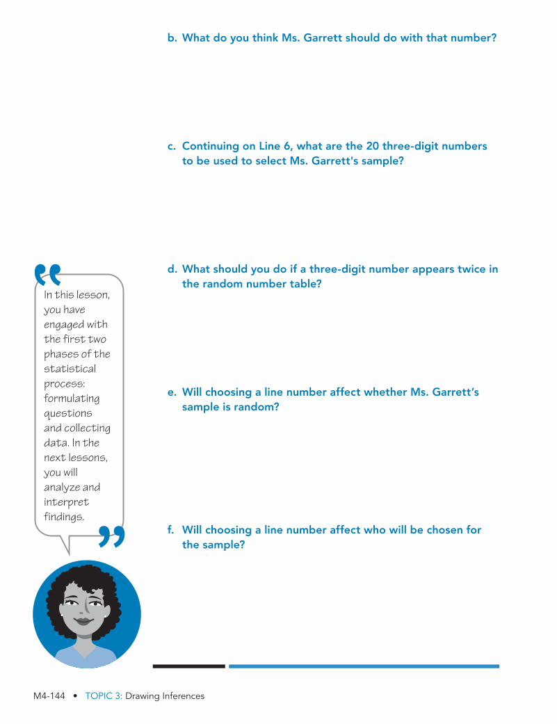
b. What do you think Ms. Garrett should do with that number?

c. Continuing on Line 6, what are the 20 three-digit numbers to be used to select Ms. Garrett's sample?

d. What should you do if a three-digit number appears twice in the random number table?

e. Will choosing a line number affect whether Ms. Garrett’s sample is random?

f. Will choosing a line number affect who will be chosen for the sample?

In this lesson, you have engaged with the first two phases of the statistical process: formulating questions and collecting data. In the next lessons, you will analyze and interpret findings.


NOTES


TALK the TALK

Lunching with Ms. Garrett

Ms. Garrett wishes to randomly select 10 students for a lunch meeting to discuss ways to improve school spirit. There are 1500 students in the school.


2. What is the sample for this problem?

3. Ms. Garrett selects three to four student council members from each grade to participate. Does this sample represent all of the students in the school? Explain your answer.

4. Ms. Levi recommended that Ms. Garrett use a random number table to select her sample of 10 students. How would you recommend Ms. Garrett assign numbers and select her random sample?



Results from a Sample Class Survey

Student1. What is your

approximate height?

2. Do you carry a cell phone with you?

3. About how many text messages do you send in one day?

1-Sue (F) 60 in. Yes 75

2-Jorge (M) 68 in. Yes 5

3-Alex (M) 63 in. No 0

4-Maria (F) 65 in. Yes 20

5-Tamika (F) 62 in. Yes 50

6-Sarah (F) 68 in. Yes 100

7-Beth (F) 56 in. Yes 60

8-Sam (M) 70 in. No 0

9-Eric (M) 69 in. Yes 50

10-Marcus (M) 66 in. Yes 100

11-Carla (F) 61 in. Yes 0

12-Ben (M) 68 in. Yes 60

13-Will (M) 64 in. Yes 50

14-Yasmin (F) 66 in. Yes 40

15-Paulos (M) 60 in. Yes 90

16-Jon (M) 67 in. Yes 10

17-Rose (F) 64 in. Yes 0

18-Donna (F) 65 in. Yes 25

19-Suzi (F) 63 in. Yes 30

20-Kayla (F) 58 in. Yes 80



Assignment

WriteMatch each definition to the corresponding term.

1. the facts or numbers gathered by a survey

2. the characteristic used to describe a sample

3. the collection of data from every member of a population

4. a method of collecting information about a certain group of people by

asking a question or set of questions

5. a sample that is selected from the population in a such a way that every

member of the population has the same chance of being selected

6. the characteristic used to describe a population

7. the entire set of items from which data can be selected

8. the data collected from part of a population

RememberStatistics obtained from data collected through a random sample are more likely to be

representative of the population than those statistics obtained from data collected through

non-random samples.

a. census

b. data

c. parameter

d. population

e. sample

f. statistic

g. survey

h. random sample

Practice

1. Explain which sampling method is more representative of the population.

a. Katie and Cole live in Springfield, RI, and are interested in the average number of skateboarders who

use their town’s Smooth Skate Park in one week. Katie recorded the number of skateboarders who

used the park in June. Cole recorded the number of skateboarders who used the park in January.

b. Fiona and Rachel want to determine the most popular lunch choice in the school cafeteria among

seventh graders. They decide to collect data from a sample of seventh graders at school. Fiona

surveys twenty seventh graders that are in line at the cafeteria. Rachel surveys twenty seventh

graders whose student ID numbers end in 9.

2. The coach of the soccer team is asked to select 5 students to represent the team in the Homecoming

Parade. The coach decides to randomly select the 5 students out of the 38 members of the team.

a. What is the population for this problem?

b. What is the sample for this problem?

c. Suggest a method for selecting the random sample of 5 students.


3. Consider the population of integers from 8 to 48.

a. Select a sample of 6 numbers. Is this a random sample? Explain your reasoning.

b. How can you assign random numbers to select a sample using a random number table?

c. Use the random number table to choose 6 numbers from this population.

d. Use a different line of the random number table to choose 6 numbers from this population.

e. Compare the results from each sample. Do the results surprise you? Explain.

4. The manager of the Millcreek Mall wants to know the mean age of the people who shop at the mall

and the stores in which they typically shop. Dennis has been put in charge of collecting data for

the Millcreek Mall. He decides to interview 100 people one Saturday because it is the mall’s busiest

shopping day.

a. What is the population for this situation?

b. What is the sample?

c. When Dennis calculates the mean age of the people who shop at the mall, will he be calculating a

parameter or a statistic? Explain your reasoning.

d. Describe three different ways Dennis can take a sample. Describe how any of these three possible

samples may cause the results of Dennis’s survey to inaccurately reflect the average age of shoppers

at the mall.

e. Dennis decides to use a random number table to choose the next 10 people to interview. Explain

how to choose 10 two-digit numbers between 1 and 80 from a random number table.

f. Record the numbers of the people who would be interviewed. Be sure to specify which line you used

to generate your list.

g. Suppose Dennis uses a random number table to generate his sample, resulting in Dennis interviewing

10 people who all go into the gaming store. Does this mean the sample is not random? Explain.

StretchVariations of random samples are often preferred to truly random samples. Two variations are called

stratified random samples and systematic random samples. Research each type of random sampling.

Define each type of sample and give an example, perhaps from the lesson, of when each might provide a

more representative sample than a truly random sample.




Review1. A soccer player makes 4 out of every 5 penalty shots she attempts.

a. What might be a good model for simulating the number of shots the soccer player makes in when

attempting 4 penalty shots?

b. Describe how you would assign outcomes and then describe one trial of the simulation.

c. Conduct 20 trials of the simulation and record your results in a table.

d. According to your simulation, what is the probability that the soccer player makes exactly 3 out of the

next 4 penalty shots?

2. Mike spins two spinners. The first spinner is divided into 4 equal sections and each is labeled with a

perfect square (4, 9, 16, 25). The second spinner is divided into 5 equal sections and each is labeled with

an even number (2, 4, 6, 8, 10).

a. Create an array to illustrate the possible products of the result of spinning both spinners.

b. What is the probability that the product is a perfect square?

c. What is the probability that the product is a perfect cube?

d. What is the probability that the product is a multiple of 10?

3. Solve each equation for the unknown.

a. 7 2 2(3t 1 9) 5 247

b. 22.5 5 (5.5h 2 7)

________ 1.5 1 4


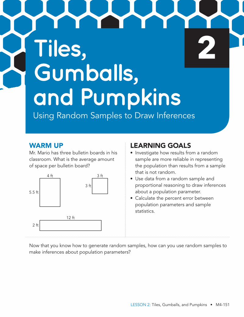
LESSON 2: Tiles, Gumballs, and Pumpkins • M4-151

LEARNING GOALS• Investigate how results from a random

sample are more reliable in representing the population than results from a sample that is not random.

• Use data from a random sample and proportional reasoning to draw inferences about a population parameter.

• Calculate the percent error between population parameters and sample statistics.

Now that you know how to generate random samples, how can you use random samples to make inferences about population parameters?

WARM UPMr. Mario has three bulletin boards in his classroom. What is the average amount of space per bulletin board?

Tiles, Gumballs, and PumpkinsUsing Random Samples to Draw Inferences

2

4 ft

5.5 ft

3 ft

3 ft

12 ft

2 ft



Getting Started

Selecting Squares

The Art Club created a design on the floor of the art room. Each of the 40 numbered squares on the floor will have colored tiles. The club needs to calculate how many colored tiles they must buy. Each small grid square represents a square that is one foot long and one foot wide.

#1#10

#12#13

#9

#2#3

#4

#8 #11

#15#14

#20

#6

#24

#38

#39#37

#28

#40

#25

#18

#5

#19

#26

#7#16

#17

#22

#29

#30

#31

#36#35

#34

#33

#32

#27

#23

#21

The Art Club needs to complete the art room floor plan project by tomorrow! Because they are short of time, they decide they do not have enough time to measure all 40 squares.

1. Suggest a method for the Art Club to use to sample the 40 squares. What would they do once they collect their sample?



Using Multiple Samples to

Make Predictions

ACTIVIT Y

2.1

Samantha says, “Since we don’t have a lot of time, why don’t we just select 5 squares and calculate their total area? That should be good enough for us to estimate the total area of all the squares that will need colored tiles.”

1. Do you think Samantha’s idea could work to estimate the total area for all the squares that need colored tiles? Explain your reasoning.


WORKED EXAMPLE

As you learned, you can select a sample to estimate parameters of a population. In this problem situation, the Art Club is going to set up a ratio using the sample of squares they select to the total area of those sample squares.

They will use the ratio:

number of squares in the sample : total area of the sample squares.

Samantha decides to select the following squares: 1, 15, 21, 37, and 40.

Total area Ratio

#1: 1 3 1 5 1 square foot

#15: 2 3 2 5 4 square feet

#21: 7 3 7 5 49 square feet

#37: 4 3 4 5 16 square feet

#40: 2 3 2 5 4 square feet

So, the total area of these 5 squares is 74 square feet.

I wonder why Samantha picked those squares.

number of squares : in the sample

5 squares : 74 square feet

total area of the sample squares



3. Select 5 numbered squares that you think best represent the 40 squares that need colored tiles. Record the numbers of the squares you selected.

4. Calculate the total area of the 5 numbered squares you selected.

Now that you have collected your data, you need to analyze the data. Remember, there are three common distributions of data: skewed left, skewed right, and symmetric. The distribution of data can help you determine whether the mean or median is a better measure of center. Examine the diagrams shown.

You will use these descriptions throughout this lesson.

The mean of a dataset is greater thanthe median whenthe data are skewedto the right.

skewed right

X X

XXX X

The median is thebest measure ofcenter because themedian is notaffected by verylarge data values.

symmetric

The mean andmedian are equalwhen the data aresymmetric.

skewed left

The mean of a data setis less than the medianwhen the data areskewed to the left.

The median is thebest measure ofcenter because themedian is notaffected by verysmall data values.

median median median

mean mean mean

The median is not affected by very large or very small data values, but the mean is affected by these large and small values.



5. Compare the total area of your sample to the total areas of your classmates’ samples.

a. Record the total area you calculated for your sample on the dot plot shown. Then, record the total areas your classmates calculated on the same dot plot.

10 20 30 40 50 60 70 80 90 100 110 120 130Total Area of the Sample Numbered Squares (sq ft)

b. Describe the distribution of the dot plot.

c. Estimate the total area for a sample of 5 squares using the data values in the dot plot.

You can set up a ratio of the sample of 5 squares to the total area of those 5 sample squares, as Samantha did, and then you can set up a proportion to estimate the total area of those 40 squares in the Art Club’s floor plan design. In doing so, you are scaling up from your sample to the population of the squares.

6. Write a ratio of the number of squares in your sample to the total area of the squares.

7. Estimate the total area of all 40 squares on the fl oor plan using proportional reasoning.



8. Compare the estimated total area of the 40 squares on the fl oor plan with your classmates’ estimated total areas.

a. Record the estimated total area of the 40 squares on the floor plan on the dot plot shown. Then, record your classmates’ estimates of the total area of the 40 squares.

b. Describe the shape of the distribution. Compare with the distribution in Question 5.

c. Estimate the total area of the squares in the floor plan using data values in the dot plot.

Total Area of All Squares (sq ft)50 150 250 350 450 550 650 750 850 950 1050



Using Random Samples

to Make Predictions

ACTIVIT Y

2.2

Samples chosen by looking at the squares and trying to pick certain squares will probably contain many more of the larger squares in the floor plan. Most of the squares actually have small areas (17 of the 40 squares have an area of 1 square foot, and 10 of the 40 squares have an area of 4 square feet); therefore, you need to use another method to randomly choose squares.

1. How might you randomly choose 5 squares for your sample?

2. Soo Jin has a suggestion on how to randomly select the numbered squares. She says, “I can cut out the squares from the fl oor plan, and then I can put these squares in a bag. That will help me randomly select squares.” Will Soo Jin’s method result in a random sample? Explain your reasoning or suggest a way to modify her strategy.

3. How can you use the random number table to choose 5 numbered squares for your sample?

When you chose your squares in the last activity, did you generate a random sample?



Please record the line number you used as a starting point for your sample.

4. Use a random number table to choose 5 numbered squares using two-digit numbers ranging between 01 and 40. Record the square numbers.

5. Calculate the total area of the 5 numbered squares you selected.

6. Compare the total area of your sample to the total areas your classmates calculated from their random samples.

a. Record the total areas your classmates calculated and the total area you calculated on the dot plot shown.

b. How do the values plotted on this dot plot compare to the values plotted in the previous activity? Compare the shapes and the centers of the data values for both dot plots.

10 20 30 40 50 60 70 80 90 100 110 120 130Area of Sample Squares (sq ft)



7. Using proportional reasoning, estimate the total area of all 40 squares on the fl oor plan using the area you calculated from the random sample.

8. Compare your estimated total area from the random sample for all 40 squares with your classmates’ total area estimates.

a. Record your estimated total area of the 40 squares on the dot plot shown. Then, record your classmates’ estimates of the total area of the 40 squares on the dot plot.

Total Area of Squares on Floor Plan50 150 250 350 450 550 650 750 850 950 1050

b. Estimate the total area of the squares in the floor plan using data values in the dot plot.

c. How do the values plotted on this dot plot compare to the values plotted in Activity 2.1, Question 8? Compare the distributions and the centers of the data values for both dot plots.



9. The actual total area of the 40 numbered squares is 288 square feet.

a. Is 288 a parameter or a statistic? Explain your reasoning.

b. Locate 288 on each dot plot you created in the previous activity and this activity. What do you notice?

c. Calculate the percent error for the parameter and your statistics from this activity and the previous activity for the total sum of the areas of the squares.

d. Based on your percent error, which sample is more accurate? Is this what you expected? Explain your reasoning.

Percent error is the

absolute value of the

ratio of the difference

between the statistic

and parameter to the

parameter.



Using Samples to Justify

Predictions

ACTIVIT Y

2.3

The student council holds regular fundraisers to raise money for community service projects. To raise money for Back-to-School Backpacks for the local homeless shelter, they hold a Gumball Guessing Competition. They place differently colored gumballs in a large, clear gumball machine. Students pay $1.00 to predict the percent of blue gumballs in the machine. Any students who predict within 5% of the actual percent win a $5.00 credit at the school store and a share of the gumballs.

To make their predictions, students take a sample of 25 gumballs (and then return the gumballs to the machine) and use the percent of blue gumballs in the sample to make their guess. The results from the first 100 students’ samples are provided in the table.

1. Create a dot plot of the results. Be sure to label your dot plot.

2. Use the results to predict the likely percent of gumballs that are blue. Explain your reasoning.

3. How many of the students obtained a sample that was less than 25% blue gumballs?

0.0 0.1 0.2 0.3 0.4 0.5 0.6 0.7 0.8 0.9 1.0

Percent of Blue

Gumballs in the Sample

Number of Samples

12% 5

16% 8

20% 13

24% 13

28% 16

32% 18

36% 13

40% 10

44% 3

48% 1



4. The gumball machine holds 10,000 gumballs and there are 2936 blue gumballs in the machine.

a. How many students will split the gumballs? How many gumballs will each student receive?

b. Is it reasonable that none of the estimates were equal to the actual percent of blue gumballs? Explain your reasoning.

c. Suppose a disgruntled student argued that there must be at least 40% blue gumballs. Use the analysis to explain why this is unlikely.

d. The principal did not take a random sample to create his estimate. Instead, he based his estimate on a visual inspection of the gumball machine. His guess was 35%. Calculate the percent error of the principal’s guess from the true percent of blue gumballs.


NOTES


TALK the TALK

Pumpkin Patch

Right before pumpkin picking season, you are hired by Paula’s Pumpkin Patch. Your first task is to determine the number of pumpkins available for picking. In addition to growing pumpkins in the pick-your-own field, Paula also grows gourds.

The diagram on the next page shows the field that contains the pumpkins and the gourds. The stars represent the gourds. Notice that there are also gaps in the field.

You and Paula agree that it would take too long to count all the pumpkins in the field.

1. Design and carry out a method to estimate the total number of pumpkins in the field without counting all the shapes. Then prepare a presentation for your classmates that includes an explanation of your method, your results, and justification of your estimate.


Pumpkins and Gourds



Assignment


PracticeThe table at the end of this assignment shows the names and ages at inauguration of 45 presidents of the

United States.

1. You want to determine the mean age of the U.S. presidents at their inaugurations. Instead of calculating

the mean using all 45 presidents’ ages, you will take a sample.

a. What is the population for this situation?

b. Select 10 presidents whose ages best represent the mean age of a U.S. president at inauguration.

c. Record the ages of these presidents.

d. Explain why you chose these presidents.

e. Is this a random sample? Explain your reasoning.

f. Calculate the mean age of the presidents you selected. Round to the nearest year.

g. Record the mean age you calculated and the mean age your classmates calculated on a dot plot.

h. Describe the distribution of the dot plot in part (g).

2. You decide to use another method to choose presidents.

a. Randomly select 10 presidents. Record the ages of these presidents.

b. Is this a random sample? Explain your reasoning.

c. Calculate the mean age of the presidents you selected. Round to the nearest year.

d. Is the mean age of the 10 presidents you selected a statistic or parameter? Explain your reasoning.

e. Record the mean age you calculated and the mean age your classmates calculated on a dot plot.

f. Describe the distribution of the line plot in part (e).

g. Calculate the actual mean age at inauguration of all 45 presidents. Round to the nearest year. Plot this

age with an A on the dot plot in part (e).

h. Calculate the percent error between the statistic from your random sample and the true mean age.

3. Why is a random sample more desirable than a sample that is not chosen randomly?

RememberIf you are estimating a parameter that is a count, rather than a

percentage, you can use proportional reasoning to scale up

from the ratio of the number of observations in your sample

to the statistic.

WriteExplain the purpose and process

of taking a sample when you are

interested in a characteristic of

the population.



Review1. Ms. Patel, the sponsor of the spirit team, wants to survey the team about upcoming events. Which

sampling methods would result in representative samples? Explain your reasoning.

a. Surveying the first 5 members who arrive at the volleyball game.

b. Drawing 5 names from a box that contains the names of all the members and surveying those 5

members.

c. Surveying the 5 members who have been members the longest.

2. Mike spins each spinner one time. He determines the

product of the two numbers.

a. Create an array to illustrate the possible products.

b. What is the sample space?

c. Determine P(multiple of 10).

d. Determine P(0).

3. A game requires spinning a spinner numbered

1 through 5 and rolling a six-sided number cube.

a. Determine the possible outcomes for playing

the game.

b. What is the probability of spinning an even number

and rolling an even number?

c. What is the probability of spinning a 5 or rolling a 5?

4. Evaluate the expression 1.2(x 1 0.9) 2 10.8 for each unknown.

a. x 5 25.5 b. x 5 8.9

StretchDesign a simulation that takes 100 samples of size 25 from a population in which 42% of the members of the

population have a particular characteristic (e.g., blood group). Formulate a question and collect the data.

For each sample, compute the percentage of observations with the given characteristic. Then analyze your

results: summarize your sample percentages in a table and on a dot plot. Interpret the results: What are

some predictions or generalizations about the population parameter based on your sample?

5

0 10

1

45

3

2

0

1

2

34

5



Presidents of the United States

President Age at Inauguration President Age at

Inauguration

George Washington 57 Franklin Pierce 48

John Adams 61 James Buchanan 65

Thomas Jefferson 57 Abraham Lincoln 52

James Madison 57 Andrew Johnson 56

James Monroe 58 Ulysses S. Grant 46

John Quincy Adams 57 Rutherford B. Hayes 54

Andrew Jackson 61 James A. Garfield 49

Martin Van Buren 54 Chester A. Arthur 51

William Henry Harrison 68 Grover Cleveland 47

John Tyler 51 Benjamin Harrison 55

James K. Polk 49 Grover Cleveland 55

Zachary Taylor 64 John F. Kennedy 43

William McKinley 54 Lyndon B. Johnson 55

Theodore Roosevelt 42 Richard Nixon 56

William Howard Taft 51 Gerald Ford 61

Woodrow Wilson 56 Jimmy Carter 52

Warren G. Harding 55 Ronald Reagan 69

Calvin Coolidge 51 George H.W. Bush 64

Herbert Hoover 54 Bill Clinton 46

Franklin D. Roosevelt 51 George W. Bush 54

Harry S. Truman 60 Barack Obama 47

Dwight D. Eisenhower 62 Donald Trump 70

Millard Fillmore 50


LESSON 3: Spicy or Dark? • M4-169

WARM UPThe dot plot shows the number of football games boys and girls attended. The "o" represents boys' responses, and the "x" represents girls' responses.

10 11 12

X X

8 90 1 32 4 5 6 7

X X

1. Estimate the mean number of games the boys attended.

2. Estimate the mean number of games the girls attended.

3. What observations can you make from your estimations of the data?

LEARNING GOALS• Calculate the measures

of center and measures of variability for two populations.

• Compare the measures of center to the measures of variability for two populations.

• Informally assess the degree of overlap of two numerical data distributions.

Spicy or Dark?Comparing Two Populations

3

You have used measures of center and measures of variation to analyze single data sets. How can you use statistics to compare two different data sets in terms of their measures of center and variation?



Getting Started

Couch Potatoes

Several teenagers were surveyed to determine the number of hours they spend watching TV during a typical weekend. Another group was surveyed about the number of hours they spend playing outside. Eight surveys were randomly chosen from each group.

The IQR is the

difference between

the third quartile and

the first quartile. The

MAD is the mean of

the absolute values of

the deviations of each

data point from

the mean.

1. Create a dot plot for each data set.

2. Calculate the mean, median, interquartile range (IQR), and mean absolute deviation (MAD) for each data set.

3. What do these measures of center and variation tell you about the data from the surveys?

Survey Number

Hours Spent Watching TV (Per Weekend)

1 5

2 3

3 10

4 6

5 15

6 9

7 8

8 3

Survey Number

Hours Spent PlayingOutside (Per Weekend)

1 1

2 2

3 0

4 3

5 8

6 2

7 3

8 3



Comparing Measures

of Center and Variation

Jessica has just opened a new restaurant, Choco-Latta, which serves nothing but chocolate milk. She is experimenting with two new flavors—a spicy chocolate milk and a dark chocolate milk.

Jessica has asked you to provide a report analyzing customer feedback about the new flavors. You have conducted a survey of 20 random customers, asking each customer to rate a flavor on a scale of zero to one hundred.

ACTIVIT Y

3.1

Flavor Rating Flavor Rating

Spicy 50 Spicy 70

Dark 20 Dark 30

Dark 30 Dark 40

Spicy 100 Spicy 70

Spicy 60 Dark 20

Spicy 80 Dark 60

Spicy 60 Spicy 80

Dark 10 Dark 20

Dark 30 Spicy 60

Dark 40 Spicy 70

The 4 steps of the statistical process are 1. Formulate a statistical question.2. Collect data.3. Analyze the data.4. Interpret the data.



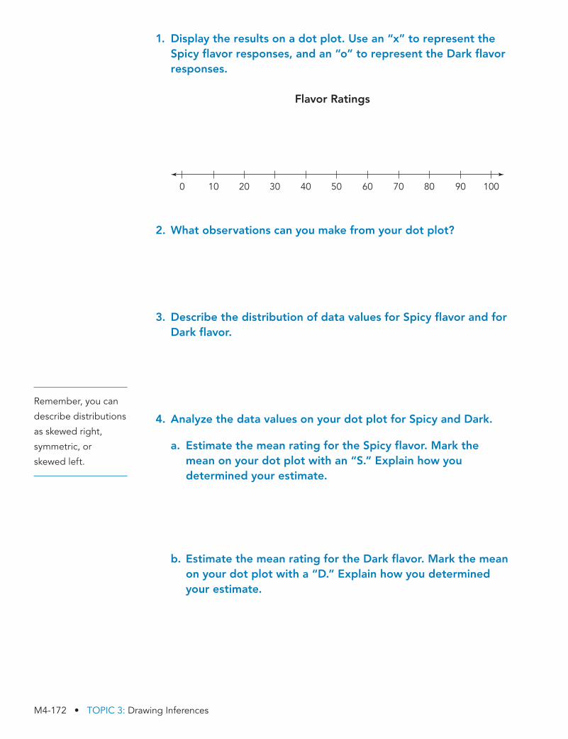
1. Display the results on a dot plot. Use an “x” to represent the Spicy flavor responses, and an “o” to represent the Dark flavor responses.

Flavor Ratings

0 10 20 30 40 50 60 70 80 90 100

2. What observations can you make from your dot plot?

3. Describe the distribution of data values for Spicy flavor and for Dark flavor.

4. Analyze the data values on your dot plot for Spicy and Dark.

a. Estimate the mean rating for the Spicy flavor. Mark the mean on your dot plot with an “S.” Explain how you determined your estimate.

b. Estimate the mean rating for the Dark flavor. Mark the mean on your dot plot with a “D.” Explain how you determined your estimate.

Remember, you can

describe distributions

as skewed right,

symmetric, or

skewed left.



5. Calculate the actual mean rating for the Spicy flavor.

6. Calculate the actual mean rating for the Dark flavor.

7. What observations can you make about the spread of the two data sets?

8. Calculate the mean absolute deviation for the ratings of the Spicy flavor and the Dark flavor.

9. Interpret and compare the mean absolute deviations for the Spicy flavor and the Dark flavor.

10. How can you tell by looking at your dot plot that the mean absolute deviations would be equal for the Spicy flavor and the Dark flavor?


NOTES


11. Can you report on which flavor has a more consistent rating? Explain your reasoning.

WORKED EXAMPLE

Comparing the difference of means with the variation in each data set can be an important way of determining just how different two data sets are.

Consider these data sets.

5, 3, 4, 5, 10 5, 3, 100, 5, 10

Mean 5 5.4 Mean 5 24.6

The difference in their means is 19.2. Depending on what you are measuring, that can be a big difference.

But this difference of 19.2 is actually less than the mean absolute deviation of the right data set (30.16). This indicates that the data sets may overlap. The right data set is the same as the left one except for one number.

12. For the Spicy flavor and Dark flavor data, compare the difference in the means with each mean absolute deviation. What observations can you make?

13. What recommendation will you give to Jessica about the two new flavors?


NOTESComparing Distributions

ACTIVIT Y

3.2

In 2009, the Los Alamos Middle School’s football team won only 2 games. The school decided to give the coach another chance at improving the team the next year. In 2010, the team won 7 games. Did scoring points have something to do with Los Alamos improving their record? The stem-and-leaf plot shows the number of points scored in each game by Los Alamos Middle School’s football team in 2009 and 2010.

Los Alamos Middle School Football Team

Points scored 2009 Points scored 2010

7 3 0 0

7 4 4 2 0 1 4 7 7

9 8 2 4 7 8 8

5 3 5 8

4 2 5

Key 5 0 1 4 means 10 and 14

1. In which year did the Los Alamos Middle School football team score more points?

2. Describe the distribution of the stem-and-leaf plots for each year.




3. Create a combined dot plot to represent the data. Use "x"s and "o"s to represent data from the different years.

Points Scored by Los Alamos Middle School Football Team, 2009 and 2010

403530 452520151050

a. How does the shape of the stem-and-leaf plot distribution compare with the shape of the dot plot distributions?

4. Determine the five number summary and IQR for each data set. Then, complete the table shown.

2009 2010

Minimum

Q1

Median

Q3

Maximum

IQR



5. In order to calculate the five number summary and IQR, did you use the data from the stem-and-leaf plot or the dot plots? Explain.

6. Compare the median and the IQR for the two data sets.

7. How does the difference in the medians compare to the IQR?

8. Do you think that scoring more points may have been one reason the Los Alamos Middle School football team improved its record?

The final step in the

statistical process is

to interpret the data.


NOTESTALK the TALK

Summarize

Write 1–2 paragraphs to summarize this lesson. Answer each question in your response.

1. How can you compare the mean and the spread of data for two populations from a dot plot?

2. If the measures of center for two populations are equivalent, how can the mean absolute variation show the differences in variation for two populations?



Assignment

WriteExplain how to compare the

difference of means with the

variation of two populations in

order to interpret the differences

between the two populations.

PracticeThe head librarian at the Branford Public Library

is investigating the current trends in technology

and the effects of computers and electronic books

on the loaning of books. She thinks that the users

at the library on the computers are generally

younger than the people who actually check out

books. She asks the ages of a sample of both

computer users and book borrowers. The results

are shown in the table.

1. Display the results on a dot plot. Use an “o” to

represent the computer users’ ages, and an “x”

to represent the book borrowers’ ages from the

information in the table.

2. Display the results using a stem-and-leaf plot.

Be sure to include a key.

3. Describe the distribution of data values for the

computer users and the book borrowers.

4. Calculate the mean age of the computer users

and the mean age of the book borrowers.

5. Calculate, interpret, and compare the mean

absolute deviations for both the computer users

and the book borrowers.

6. Determine the five-number summary for the

computer uses and the book borrowers.

7. Calculate, interpret, and compare the IQR

for both the computer users and the book

borrowers.

8. What can you say about these two populations?

RememberData for two populations may overlap. Comparing the measures of

center and variation for the two populations can help you interpret

the differences between the two populations.

Patron

AgeComputer

userBook

borrower

C 27

C 16

B 57

C 20

B 55

B 60

C 22

B 59

B 63

C 20

C 24

B 63

B 60

C 22

C 20

C 17

B 66

B 60

B 55

C 25



StretchLet the difference in means between two data sets be k. Let the mean absolute deviation for the first data

set be m and the mean absolute deviation for the second data set be n. Is it possible for the data sets to

overlap if both k __ m and k __ n are greater than 1? If so, provide an example.

Review1. Louie is using a computer program to randomly generate a digit from 1 to 6. Which statement most

accurately describes how many times Louie’s program will generate a 3 if he runs it 300 times? Explain

your choice.

a. exactly 50 times

b. approximately 50 times

c. exactly 100 times

d. approximately 100 times

2. The school cafeteria has a hot food line and a cold food line for both breakfast and lunch. The cafeteria

manager wants to estimate the percentage of students who select their meals from the hot food line.

The manager collected data from the first 50 students who arrive for lunch and determined that 42% of

students select their meals from the hot food line. Which statement is true about the cafeteria manager’s

sample? Explain your choice.

a. The sample is the percent of students who select foods from the hot food line.

b. The sample shows that exactly 42% of the student body select food from the hot food line.

c. The sample might not be representative of the population because it only included the first group of

lunch students.

d. The sample size is too small to make any generalizations.

3. The spinner is divided into 8 equal sections.

Determine each probability.

a. P(greater than 3)

b. P(not greater than 3)

4. Determine each difference.

a. 27.7 2 (277.7)

b. 4 1 __ 5 2 10 3 __ 4


1

25

4

2

3

1

2


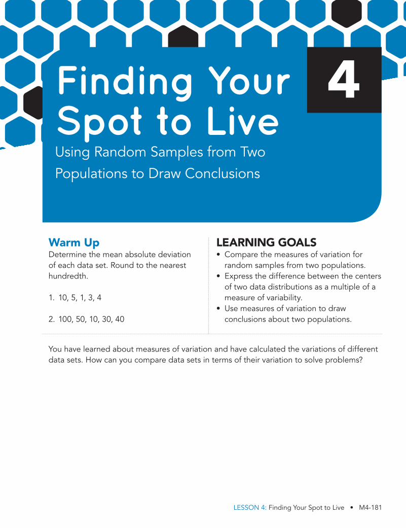
LESSON 4: Finding Your Spot to Live • M4-181

LEARNING GOALS• Compare the measures of variation for

random samples from two populations.• Express the difference between the centers

of two data distributions as a multiple of a measure of variability.

• Use measures of variation to draw conclusions about two populations.

You have learned about measures of variation and have calculated the variations of different data sets. How can you compare data sets in terms of their variation to solve problems?

Warm UpDetermine the mean absolute deviation of each data set. Round to the nearest hundredth.

1. 10, 5, 1, 3, 4

2. 100, 50, 10, 30, 40

Finding Your Spot to LiveUsing Random Samples from Two

Populations to Draw Conclusions

4



Getting Started

Downloading Podcasts

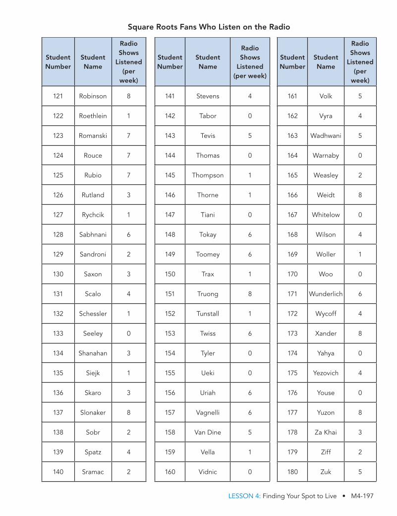
Square Roots is a radio show that airs 10 times a week on local radio station WMTH.

WMTH is trying to raise its commercial airtime rates during Square Roots. The station claims that while this music show is listened to by hundreds of middle school students via the radio, there are actually a greater number of middle school students who listen to the show by regularly downloading the podcast. Advertisers disagree with WMTH’s claim. Advertisers want the station to verify its claim that there are more students listening by downloaded podcasts than actual listeners. To do so, WMTH and the advertisers choose Bryce Middle School to collect data. They send out a survey and ask the following two questions:

• Do you listen to Square Roots on the radio or download the podcast?

• How often do you listen to Square Roots per week?

All 389 students at Bryce Middle School who listen to Square Roots responded to the survey.

1. What are the two populations for the Square Roots survey WMTH is conducting?

WMTH decides to select a random sample for each population.

2. There are 180 regular radio listeners and 209 podcast listeners at Bryce Middle School. Describe how WMTH and the advertisers can randomly select students for their sample.



Let’s use a random number table to simulate random samples from the data. The random number table and data are at the end of the lesson.

1. Use the random number table and the list of radio and podcast listeners in Bryce Middle School at the end of the lesson to help WMTH randomly select a sample.

a. Randomly select 10 radio listeners. Record each student’s last name. Then, use the list to record the number of times each student listened to Square Roots during the week.

b. Randomly select 10 podcast listeners. Record each student’s last name. Then, use the list to record the number of podcasts each student downloaded in one week.

Simulating Random SamplesACTIVIT Y

4.1

When you are assigning each student a number, each number should have the maximum number of digits in the largest number of a population.Therefore, if there are 300 people in a population, each number assigned should have three digits.



2. Construct a combined dot plot for the two groups. What conclusions can you draw?

Radio Shows and Podcasts(per week)

9 107 86543210

3. Describe the distribution for each graph. Describe any clusters or gaps in the data values in each graph.

4. Estimate the mean for each dot plot. Explain how you determined your estimate.

5. Calculate the mean number of radio shows listened to in a week, and the mean number of podcasts downloaded in a week.

6. Compare the two samples. Are more shows listened to on the radio, or are more podcasts downloaded?



7. Calculate the mean absolute deviation for each group. Compare the measures of center and variation.

8 Richard says,“If we had started on a different line number in the random number table, our results would have been the same.” Is Richard correct? Explain your reasoning.

9. Combine your data with the data from other classmates. Calculate measures of center and variation for the two combined random samples, and interpret your results.

10. Determine the difference of means for the two samples and describe this difference as a multiple of the measure of variation.

The third step in the

statistical process is

to interpret the data.



Dominique graduated from college and now has a choice of two jobs. One of the jobs is in Ashland, and the other job is in Belsano. Since Dominique enjoys mild weather and average temperatures in the 60s (8F), she decides to compare the monthly average temperatures of the two cities. She gathered the following sample of average monthly temperatures for a previous year for the two cities as shown in the table.

Month

Ashland Average Monthly

Temperatures(8F)

Belsano Average Monthly

Temperatures(8F)

January 56 48

February 58 55

March 60 59

April 61 62

May 65 66

June 70 69

July 75 78

August 82 88

September 73 82

October 68 69

November 60 59

December 56 49

Comparing Random SamplesACTIVIT Y

4.2



1. What are some ways Dominique could analyze the data to determine which city is warmer?

2. Dominique decides to calculate the mean and median temperature for each city to determine which city is warmer overall. Calculate the mean and median temperature for both cities. What do you notice?

3. Jacqui says that since Ashland and Belsano have very similar mean and median temperatures, Dominique could choose either city to live in because they both have mild temperatures. Do you agree or disagree? Explain your reasoning.



4. Construct a back-to-back stem-and-leaf plot for the average monthly temperature for each city.

Ashland Belsano

5. What conclusions can you draw from the plot?

6. Determine and interpret the five number summary and IQR for each data set. Then, describe some observations from the data of each five number summary.

Ashland Belsano

Minimum:

Q1:

Median:

Q3:

Maximum:

IQR:

Don't forgetto add a keyto the plot.


NOTES


7. Construct and label box-and-whisker plots for each data set using the same number line for both. What conclusions can you make?

9080 8575706560555045

8. Compare the mean and variation of the samples. If you were Dominique, which city would you choose to live in? Explain your reasoning.



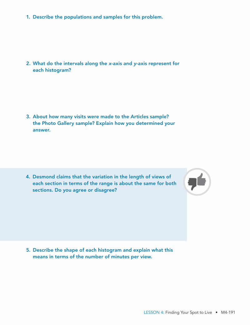
Web sites often analyze customer visits to see if there are patterns or trends. Gaining information about patterns helps companies display the information users want.

A sample of customer visits to Horizon, a news and opinion website, are shown in the histograms. The histograms display the number of visits customers made to the Articles and Photo Gallery sections of the website, along with how long each customer spent viewing content in each section.

Minutes per View5 10 15 20 25 30 35 40 45 50

250

200

150

100

50

00

Num

ber

of

Vis

its

Visits to the Articles

00

50

100

150

200

250

300

Num

ber

of

Vis

its

Minutes per View

Visits to the Photo Gallery

5 10 15 20 25 30 35 40 45 50

Analyzing Displays of Data

from Random Samples

ACTIVIT Y

4.3



1. Describe the populations and samples for this problem.

2. What do the intervals along the x-axis and y-axis represent for each histogram?

3. About how many visits were made to the Articles sample? the Photo Gallery sample? Explain how you determined your answer.

4. Desmond claims that the variation in the length of views of each section in terms of the range is about the same for both sections. Do you agree or disagree?

5. Describe the shape of each histogram and explain what this means in terms of the number of minutes per view.



6. Determine whether the mean or the median is greater for each section. Then, explain why that measure of center is greater in value for each section.

7. If you calculate the mean absolute deviation for the length of the views, which section would have more variation in the length of views? Why?

8. The box-and-whisker plots shown represent the view durations for the Photo Gallery and Articles sections. Using the information you know from the histograms for each section, which box plot do you think represents the view durations for Articles, and which represents the view durations for Photo Gallery? Explain your choice.

0 50 0 50

9. In terms of the box-and-whisker plots, which section has more variation in the duration of views? Explain your reasoning.


NOTES


TALK the TALK

Into Each Life Some Rain Must Fall

Sam lives in Seattle, Washington, and says it seems like it rains all the time. Richard lives in Washington, D.C., and says it seems like it doesn’t rain very much.

The table contains the average monthly rainfall for both cities over the past 30 years.

1. Use any method you want to determine the validity of Sam's and Richard's statements.

Month

Seattle, Washington

Average Monthly Rainfall (inches)

Washington, D.C. Average

Monthly Rainfall (inches)

January 5.24 3.21

February 4.09 2.63

March 3.92 3.60

April 2.75 2.77

May 2.03 3.82

June 1.55 3.13

July 0.93 3.66

August 1.16 3.44

September 1.61 3.79

October 3.24 3.22

November 5.67 3.03

December 6.06 3.05



Square Roots Fans Who Listen on the Radio

Student Number

Student Name

Radio Shows

Listened (per

week)

Student Number

Student Name

Radio Shows

Listened(per week)

Student Number

Student Name

Radio Shows

Listened(per

week)

1 Abunto 1 21 D’Ambrosio 0 41 Granger 0

2 Adler 3 22 Datz 4 42 Guca 2

3 Aizawa 3 23 Delecroix 2 43 Haag 8

4 Alescio 4 24 Difiore 6 44 Heese 5

5 Almasy 8 25 Dobrich 7 45 Hilson 1

6 Ansari 6 26 Donoghy 1 46 Holihan 1

7 Aro 7 27 Donaldson 5 47 Hudack 1

8 Aung 2 28 Dreher 2 48 Ianuzzi 3

9 Baehr 7 29 Dubinsky 1 49 Islamov 4

10 Bellmer 1 30 Dytko 8 50 Jacobsen 5

11 Bilski 4 31 Fabry 7 51 Jessell 4

12 Blinn 6 32 Fetcher 1 52 Ji 1

13 Bonetto 3 33 Fontes 5 53 Johnson 2

14 Breznai 1 34 Frick 3 54 Jomisko 1

15 Cabot 3 35 Furmanek 5 55 Jones 6

16 Chacalos 0 36 Gadgil 4 56 Joy 5

17 Cioc 0 37 Gavlak 4 57 Jumba 1

18 Cole 3 38 Gibbs 0 58 Juth 7

19 Creighan 4 39 Gloninger 2 59 Jyoti 6

20 Cuthbert 6 40 Goff 1 60 Kachur 2




Student Number

Student Name

Radio Shows

Listened (per

week)

Student Number

Student Name

Radio Shows

Listened(per week)

Student Number

Student Name

Radio Shows

Listened(per

week)

61 Kanai 0 81 McNary 7 101 Nzuyen 2

62 Keller 2 82 Meadows 0 102 O’Bryon 0

63 Khaing 7 83 Merks 8 103 Obitz 3

64 Kindler 5 84 Mickler 5 104 Oglesby 8

65 Kneiss 5 85 Minniti 4 105 Ono 1

66 Kolc 1 86 Mohr 3 106 Paclawski 0

67 Kuisis 2 87 Mordecki 5 107 Pappis 6

68 Labas 1 88 Mueser 3 108 Peery 3

69 Lasek 8 89 Musati 3 109 Phillips 5

70 Leeds 5 90 Myron 2 110 Potter 3

71 Lin 0 91 Nadzam 4 111 Pribanic 7

72 Litsko 2 92 Nazif 7 112 Pwono 5

73 Lodi 3 93 Newby 0 113 Quinn 2

74 Lookman 2 94 Ng 1 114 Rabel 5

75 Lucini 1 95 Nino 2 115 Rayl 2

76 Lykos 0 96 Northcutt 4 116 Rea 4

77 MacAllister 1 97 Novi 3 117 Reynolds 5

78 Magliocca 6 98 Null 8 118 Rhor 8

79 Marchick 5 99 New 5 119 Rielly 8

80 McGuire 1 100 Nyiri 1 120 Risa 7




Student Number

Student Name

Radio Shows

Listened (per

week)

Student Number

Student Name

Radio Shows

Listened(per week)

Student Number

Student Name

Radio Shows

Listened(per

week)

121 Robinson 8 141 Stevens 4 161 Volk 5

122 Roethlein 1 142 Tabor 0 162 Vyra 4

123 Romanski 7 143 Tevis 5 163 Wadhwani 5

124 Rouce 7 144 Thomas 0 164 Warnaby 0

125 Rubio 7 145 Thompson 1 165 Weasley 2

126 Rutland 3 146 Thorne 1 166 Weidt 8

127 Rychcik 1 147 Tiani 0 167 Whitelow 0

128 Sabhnani 6 148 Tokay 6 168 Wilson 4

129 Sandroni 2 149 Toomey 6 169 Woller 1

130 Saxon 3 150 Trax 1 170 Woo 0

131 Scalo 4 151 Truong 8 171 Wunderlich 6

132 Schessler 1 152 Tunstall 1 172 Wycoff 4

133 Seeley 0 153 Twiss 6 173 Xander 8

134 Shanahan 3 154 Tyler 0 174 Yahya 0

135 Siejk 1 155 Ueki 0 175 Yezovich 4

136 Skaro 3 156 Uriah 6 176 Youse 0

137 Slonaker 8 157 Vagnelli 6 177 Yuzon 8

138 Sobr 2 158 Van Dine 5 178 Za Khai 3

139 Spatz 4 159 Vella 1 179 Ziff 2

140 Sramac 2 160 Vidnic 0 180 Zuk 5



Square Roots Fans Who Download Show Podcasts

Student Number

Student Name

Podcasts Downloaded (per week)

Student Number

Student Name


Student Number

Student Name


1 Aaronson 2 21 Chang 4 41 Frena 1

2 Abati 0 22 Clarke 9 42 Galdi 8

3 Ackerman 4 23 Crnkovich 0 43 Gansberger 3

4 Aderholt 2 24 Dahl 0 44 Gianni 1

5 Akat 7 25 Dax 7 45 Glencer 1

6 Aleck 9 26 Defoe 1 46 Godec 7

7 Alessandro 5 27 Dengler 4 47 Goldstein 0

8 Allen 3 28 Di Minno 4 48 Graef 6

9 Ansil 1 29 Dilla 5 49 Gula 1

10 Archer 5 30 Draus 5 50 Hagen 2

11 Badgett 9 31 Duffy 0 51 Haupt 8

12 Bartle 2 32 Ecoff 3 52 Herc 4

13 Bibby 9 33 Esparra 7 53 Hnat 9

14 Bilich 5 34 Fakiro 7 54 Hodak 3

15 Bloom 3 35 Ferlan 4 55 Hoyt 2

16 Boccio 5 36 Fetherman 2 56 Huang 3

17 Bracht 3 37 Fillipelli 6 57 Iannotta 4

18 Bujak 7 38 Fisher 2 58 Irwin 5

19 Caliari 9 39 Folino 9 59 Jackson 7

20 Cerminara 8 40 Forrester 9 60 Jamil 1




Student Number

Student Name


Student Number

Student Name


Student Number

Student Name


61 Jessop 1 81 Ling 6 101 Moorey 6

62 Johnson 9 82 Loch 4 102 Mox 7

63 Joos 9 83 Lorenzo 4 103 Mrkali 7

64 Joseph 5 84 Lovejoy 5 104 Mu 0

65 Jubic 3 85 Luba 8 105 Muller 3

66 Juhl 7 86 Lukitsch 4 106 Murphy 2

67 Jung 9 87 Luzzi 8 107 Mwambazi 6

68 Jurgensen 4 88 Lyman 5 108 Myers 4

69 Jyoti 0 89 MacIntyre 8 109 Nangle 3

70 Kaib 5 90 Maddex 5 110 Neilan 7

71 Kapoor 6 91 Marai 2 111 Nicolay 5

72 Kennedy 2 92 Mato 9 112 Niehl 6

73 Kimel 5 93 McCaffrey 0 113 Nix 2

74 Klaas 4 94 McElroy 5 114 Noga 3

75 Ko 9 95 McMillan 3 115 Nowatzki 7

76 Krabb 1 96 Meng 9 116 Nuescheler 5

77 Ladley 9 97 Michelini 5 117 Nye 6

78 Lawson 1 98 Misra 0 118 Nytra 6

79 Lemieux 7 99 Miller 8 119 O’Carrol 6

80 Lewan 6 100 Modecki 7 120 Obedi 7




Student Number

Student Name


Student Number

Student Name


Student Number

Student Name


121 Oehrle 8 141 Rea 5 161 Scopaz 4

122 Olds 5 142 Renard 7 162 Sebula 4

123 Oleary 0 143 Rex 7 163 Shah 1

124 Ondrey 1 144 Richards 7 164 Sidor 6

125 Owusu 9 145 Ridout 7 165 Skraly 6

126 Palamides 9 146 Rivera 6 166 Sokolowski 5

127 Pappas 0 147 Roberts 4 167 Speer 6

128 Pecori 3 148 Rodwich 0 168 T’Ung 9

129 Pennix 4 149 Roney 7 169 Tamar 9

130 Pendleton 1 150 Ross 6 170 Tebelius 1

131 Phillippi 2 151 Rothering 0 171 Tesla 4

132 Pieton 6 152 Rua 4 172 Thuma 0

133 Ploeger 2 153 Russo 8 173 Tibi 2

134 Pressman 4 154 Ryer 8 174 Tobkes 9

135 Puzzini 1 155 Sagi 8 175 Torelli 8

136 Qu 4 156 Sallinger 6 176 Tozzi 0

137 Qutyan 8 157 Sau 7 177 Traut 6

138 Raab 5 158 Sbragia 7 178 Trax 0

139 Raeff 0 159 Schaier 5 179 Tu 8

140 Rav 1 160 Schmit 2 180 Tumicki 2




Student Number

Student Name


Student Number

Student Name


Student Number

Student Name


181 Tyson 1 191 Wallace 2 201 Wulandana 8

182 Uansa 0 192 Webb 9 202 Wysor 9

183 Ulan 4 193 Weisenfeld 0 203 Xiao 4

184 Urbano 7 194 Whalen 7 204 Yee 6

185 Uzonyi 7 195 Wiley 9 205 Yost 1

186 Vaezi 8 196 Williams 5 206 Young 7

187 Vinay 6 197 Williamson 6 207 Yuros 6

188 Vu 8 198 Witek 9 208 Zaki 0

189 Wallee 0 199 Wojcik 3 209 Zimmerman 1

190 Waldock 4 200 Woollett 6



Random Number Table

Line 1 65285 97198 12138 53010 94601 15838 16805 61004 43516 17020

Line 2 17264 57327 38224 29301 31381 38109 34976 65692 98566 29550

Line 3 95639 99754 31199 92558 68368 04985 51092 37780 40261 14479

Line 4 61555 76404 86210 11808 12841 45147 97438 60022 12645 62000

Line 5 78137 98768 04689 87130 79225 08153 84967 64539 79493 74917

Line 6 62490 99215 84987 28759 19177 14733 24550 28067 68894 38490

Line 7 24216 63444 21283 07044 92729 37284 13211 37485 10415 36457

Line 8 16975 95428 33226 55903 31605 43817 22250 03918 46999 98501

Line 9 59138 39542 71168 57609 91510 77904 74244 50940 31553 62562

Line 10 29478 59652 50414 31966 87912 87154 12944 49862 96566 48825

Line 11 96155 95009 27429 72918 08457 78134 48407 26061 58754 05326

Line 12 29621 66583 62966 12468 20245 14015 04014 35713 03980 03024

Line 13 12639 75291 71020 17265 41598 64074 64629 63293 53307 48766

Line 14 14544 37134 54714 02401 63228 26831 19386 15457 17999 18306

Line 15 83403 88827 09834 11333 68431 31706 26652 04711 34593 22561

Line 16 67642 05204 30697 44806 96989 68403 85621 45556 35434 09532

Line 17 64041 99011 14610 40273 09482 62864 01573 82274 81446 32477

Line 18 17048 94523 97444 59904 16936 39384 97551 09620 63932 03091

Line 19 93039 89416 52795 10631 09728 68202 20963 02477 55494 39563

Line 20 82244 34392 96607 17220 51984 10753 76272 50985 97593 34320



Assignment

Practice1. Repeat the sampling procedure you used with the data in Activity 4.1. Choose a different line number in

the random number table.

a. Record the results for 20 students.

b. Construct a combined dot plot for the two groups, using the same scale.

c. Describe the distribution of the data for each group.

d. Estimate and then calculate the mean for the data in each group.

e. Compare your new results with your results from Activity 4.1.

2. Ratings are not limited to television shows alone. Ratings can also be used to show people’s opinions of

hotels and restaurants. One of the things that can help a restaurant get good ratings is the time it takes

to be seated (the wait time) at a restaurant without reservations.

3. Big Al’s Steak House and Trail’s End both claim to have the shortest wait times in town. To check out the

claims, Ramon, a restaurant reviewer, records the time it takes to be seated without reservations. The

results of wait times for 8 visits to each restaurant are shown in the table.

Big Al’s Steak House Wait Times

(minutes)

Trail’s End Wait Times

(minutes)

5 11

13 19

22 14

7 14

20 15

21 20

20 10

12 17

a. Describe the populations and samples for this problem.

b. Calculate the mean wait times between the two restaurants. Which restaurant

seems to have faster service?

RememberYou can use the means and mean absolute deviations to compare

two populations with approximately symmetric data sets. You

can use the medians and the interquartile range to compare two

populations with skewed data sets.

WriteExplain how to use measures of

center and variation to compare

two populations.



c. Complete the dot plot of the times. What do you notice?

d. Determine the median wait time for each restaurant.

e. Explain the difference in median times for the two restaurants.

f. Which measure of center would you use if:

a. you are Big Al’s Steak House and want to claim you have the shortest wait time?

b. you are Trail’s End and want to claim you have the shortest wait time?

c. you are a customer and want the shortest wait time?

g. Suppose another restaurant reviewer records wait times at each restaurant several times. Do you think

it is possible that the wait times might be different from Ramon’s wait times? Explain your reasoning.

h. How could we be more certain which restaurant has the shortest wait time?

2520151050

= Big Al’s Steak House

X = Trail’s End

Wait Times

StretchConduct your own experiment! Collect data from samples drawn from two populations. Then, analyze the

data and report on your findings.

ReviewDescribe the difference in means between each data set as a multiple of the mean absolute deviation of

each data set.

1. {1, 2, 3, 4, 5} {5, 5, 5, 5, 5}

2. {62, 41, 11, 60, 55} {50, 112, 149, 131, 60}

A spinner has 6 equal sections, labeled 1 through 6. Determine each compound probability.

3. What is the probability that the next spin is a 2 or a 5?

4. What is the probability that the next spin is a 1, 2, or 3?

Evaluate each expression for x 5 20.5.

5. x4 1 x3

6. 2x4 2 x3


TOPIC 3: SUMMARY • M4-205

Drawing Inferences Summary

There are four components of the statistical process:• Formulating a statistical question.• Collecting appropriate data.• Analyzing the data graphically and numerically.• Interpreting the results of the analysis.

One data collection strategy you can use is a survey. A survey is a method of collecting information about a certain group of people. It involves asking a question or a set of questions to those people. When information is collected, the facts or numbers gathered are called data.

The population is the entire set of items from which data can be selected. When you decide what you want to study, the population is the set of all elements in which you are interested. The elements of that population can be people or objects. A census is the data collected from every member of a population.

In most cases, it is not possible or logical to collect data from every member of the popula-tion. When data are collected from a part of the population, the data are called a sample.

KEY TERMS• survey• data• population

• census• sample• parameter

• statistic• random sample

LESSON

1 We Want to Hear From You!

AL7_SE_TS_M04_T03.indd 205AL7_SE_TS_M04_T03.indd 205 1/14/19 11:59 AM1/14/19 11:59 AM

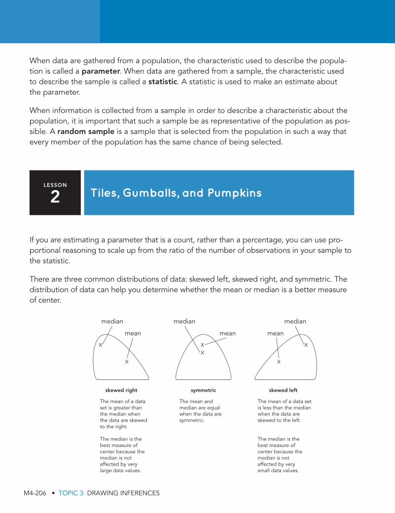
M4-206 • TOPIC 3: DRAWING INFERENCES

When data are gathered from a population, the characteristic used to describe the popula-tion is called a parameter. When data are gathered from a sample, the characteristic used to describe the sample is called a statistic. A statistic is used to make an estimate about the parameter.

When information is collected from a sample in order to describe a characteristic about the population, it is important that such a sample be as representative of the population as pos-sible. A random sample is a sample that is selected from the population in such a way that every member of the population has the same chance of being selected.

If you are estimating a parameter that is a count, rather than a percentage, you can use pro-portional reasoning to scale up from the ratio of the number of observations in your sample to the statistic.

There are three common distributions of data: skewed left, skewed right, and symmetric. The distribution of data can help you determine whether the mean or median is a better measure of center.

LESSON

2 Tiles, Gumballs, and Pumpkins

The mean of a dataset is greater thanthe median whenthe data are skewedto the right.

skewed right

X X

XXX X

The median is thebest measure ofcenter because themedian is notaffected by verylarge data values.

symmetric

The mean andmedian are equalwhen the data aresymmetric.

skewed left

The mean of a data setis less than the medianwhen the data areskewed to the left.

The median is thebest measure ofcenter because themedian is notaffected by verysmall data values.

median median median

mean mean mean


TOPIC 3: SUMMARY • M4-207

Data for two populations may overlap. Comparing the measures of center and variation for the two populations can help you interpret the differences between the two populations.

Comparing the difference of means with the variation in each data set can be an important way of determining just how different two data sets are.

For example, consider these data sets.

5, 3, 4, 5, 10 5, 3, 100, 5, 10Mean 5 5.4 Mean 5 24.6

The difference in their means is 19.2. Depending on what you are measuring, that can be a big difference. However, this difference of 19.2 is actually less than the mean absolute deviation of the right data set (30.16). This indicates that the data sets may overlap. The right data set is the same as the left one except for one number.

You can use the means and mean absolute deviations to compare two populations with approximately symmetric data sets. You can use the medians and the interquartile range to compare two populations with skewed data sets.

For example, suppose Forrest wanted to compare the number of text messages sent each day by middle school students to the number of text messages sent each day by high school stu-dents. He randomly selected and surveyed 10 students from each grade. The data sets provid-ed represent the number of text messages each student said they send each day.

Grade 7: 44, 40, 43, 73, 74, 76, 56, 59, 66, 54

Grade 8: 77, 86, 69, 52, 76, 79, 60, 61, 57, 85

LESSON

3

LESSON

4

Spicy or Dark?

Finding Your Spot to Live


M4-208 • TOPIC 3: DRAWING INFERENCES

Forrest created a back-to-back stem-and-leaf plot to display the data.

Grade 7 Grade 8

Leaf Stem Leaf

4 3 0 4

9 6 4 5 2 7

6 6 0 1 9

6 4 3 7 6 7 9

8 5 6

For grade 7, the mean number of texts sent per day is 58.5 and the mean absolute deviation is 11.1. The median is 57.5 and the interquartile range is 29. For grade 8, the mean number of texts sent per day is 70.2 and the mean absolute deviation is 10.4. The median is 69 and the interquartile range is 22.


topic 3 drawing inferences · topic 3: drawing inferences in this topic, students continue...

Documents