Tools toCharacterize andStudy Polymers.

Overview.1. Osmometry. 2. Viscosity Measurements.3. Elastic and Inelastic Light Scattering.

4. Gel-Permeation Chromatography.

5. Atomic Force Microscopy.6. Computer Simulation.

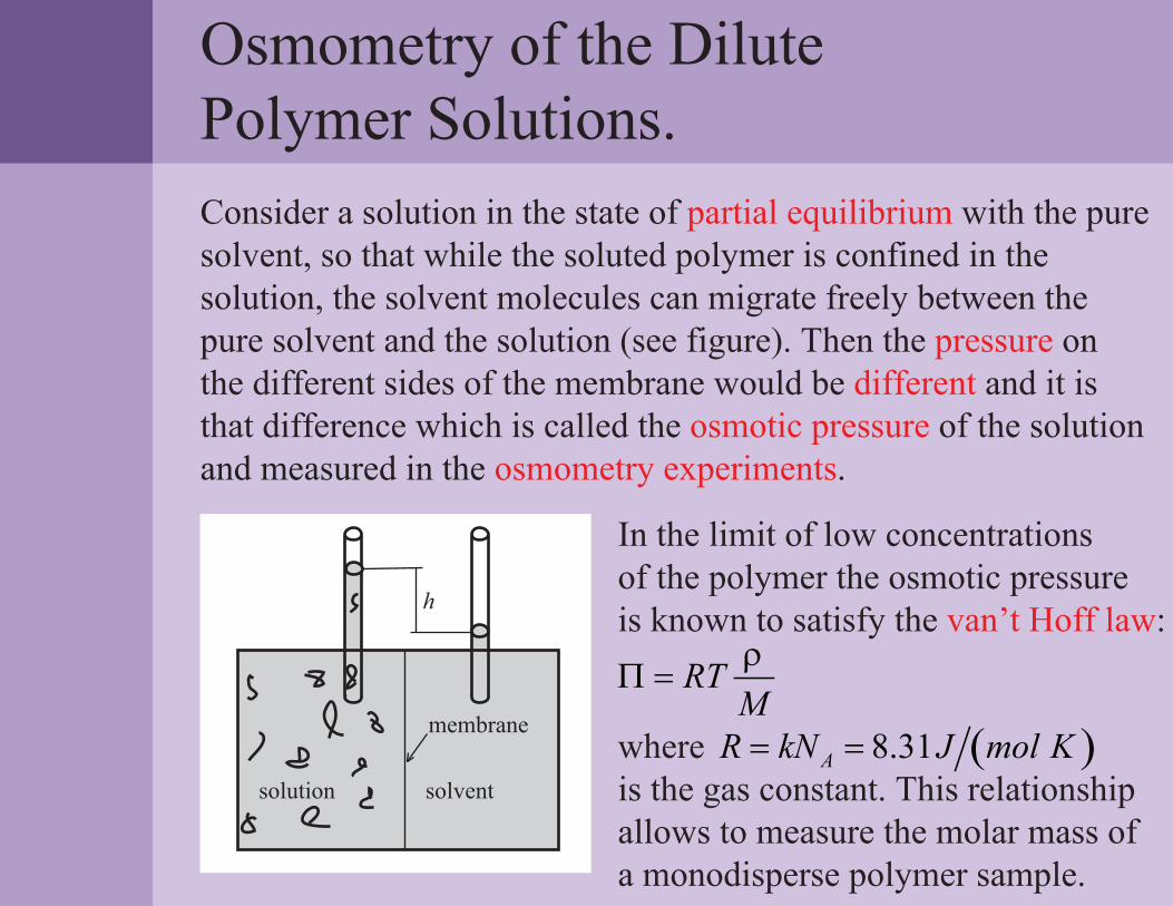
Osmometry of the Dilute Polymer Solutions.Consider a solution in the state of partial equilibrium with the puresolvent, so that while the soluted polymer is confined in the solution, the solvent molecules can migrate freely between thepure solvent and the solution (see figure). Then the pressure onthe different sides of the membrane would be different and it is that difference which is called the osmotic pressure of the solutionand measured in the osmometry experiments.

h

solution solvent

membrane

In the limit of low concentrationsof the polymer the osmotic pressureis known to satisfy the van’t Hoff law:

where is the gas constant. This relationship allows to measure the molar mass of a monodisperse polymer sample.

( )8.31AR kN J mol K= =

RTMρ

Π =

Osmometry of the Polymer Solutions. Measuring the Molecular Mass.Consider now a more complicated case of a polydisperse polymersample. Then the van’t Hoff law is to be rewritten as follows

Thus, we get the following formula

which allows to measure the number average molecular mass of apolymer sample by measuring the osmotic pressure in the dilute solution of this sample at very low concentrations.

ii

i n

RT RT c RTM Mρ ρ

Π = = =∑ ∑where are the molecular mass, density, and concentrationof the i-th fraction of the sample, respectively, while is the number average molecular mass of the sample.

, ,i i iM cρ

n i i iM c cρ ρ= =∑ ∑ ∑

0lim

n

RTMρ ρ→

Π=

Osmometry of the Polymer Solutions. Measuring the Second Virial Coefficient.The van’t Hoff law introduced above can be considered as a firstterm of a virial expansion for the osmotic pressure:

2 3, ,...A Awhere are the (properly averaged, see below) second, third, etc. virial coefficients of the coils. Note the difference between these coefficients which describe the interactions of the coils with each other, and the virial coefficients of single monomer units introduced in the previous lecture. In particular, for weak interactions , where B is the second virial coefficient of the monomer units.

22A N B

Moreover, for a polidisperse sample

where is the second virial coefficient describing the interaction of the i-th and j-th fractions.

( )2ijA

2 32 3 ...

n

A ART M

ρρ ρ

Π= + + +

( )22 2

,

1i j ij

i jA Aρ ρ

ρ= ∑

Osmometry of the Polymer Solutions. Conclusions.

Thus, in the osmometry measurements the ratio is measured as a function of polymer mass concentration ρ. By extrapolating it to the zero concentration one gets the inverse of the number average molecular mass, while the slope of the dependence at low values of ρ gives the second virial coefficient of the interactions of the coils.

21 ...

n

ART M

ρρΠ

= + +

RTρΠ

Viscosity of the Dilute Polymer Solutions.

0η

For the dilute polymer solutions, one is normally interested not in the value of η itself but in the specific viscosity (where is the viscosity of pure solvent) and the characteristic viscosity , where ρ is the density of monomer units in solution.

( )0 0sη η η η= −

[ ] ( )0 0η η η η ρ= −

For the solution of impenetrable spheres of radius R Einstein derived

( )0 1 2.5η η= + Φwhere Φ is the volume fraction occupied by the spheres in solution. If each sphere consists of N particles (monomer units) of mass m, and the average density of the spheres in the solutionis ρ, we get

3 34 43 3

A AN NR RmN Mρ ρπ π

Φ = =

where M is the molecular mass of the polymer chain, M = mN, and N is the Avogadro number.A

Viscosity of the Dilute Polymer Solutions.

[ ]3102.5

3AR N

Mπ

ηρΦ

= =

For dense spheres and [η] is independent of the size of the particles. Therefore, the viscosity measurements are not informative in this limit. E.g. for globular proteins one always obtains independently of the size of the globule.[ ] 34cm gη ≈

3N R

However, polymer coils are very loose objects with3 3 3 3 1/ 2 3

0N R N R N aα α− − −

If they still move as a whole together with the solvent inside the coil (the non-draining assumption), the Einstein formula remains valid. Then

[ ]3

3 1/ 2 3103

AR N N amN

πη α=

i.e., for polymer coils there is a non-trivial N dependence. Thus, by measuring [η] one can get information about the size of polymer coils.

Viscosity of the Dilute Polymer Solutions.Similary to the consideration of the osmotic pressure above, it ispossible to go beyond the zero-concentration limit and expandthe viscosity in powers of the concentration. The resulting formula,known as Huggins equation, is as follows

where is the so-called Huggins constant. The same result can berewritten in the different form called the Kraemer equation

Hk

In practice these two equations are used simultaneously to determinethe characteristic viscosity. When both the Huggins and Kraemer equations provide the same characteristic viscosity and Huggins constant, the high-order terms can be safely ignored. If not, viscositymeasurements need to be made at lower concentrations.

[ ] [ ]2 ...sH

s

kη ηη η ρ

η ρ−

= + +

( ) [ ] [ ]( ) [ ] [ ]2 22ln 1 1ln 1 ... ...2

sH Hk k

η ηη ρ η ρ η η ρ

ρ ρ = + + + = + − +

What Can Be Measured in Viscosimetry Experiments?1. If the measurements are performed at the Θ-point one has

[ ]3/ 22

006

S

Mη

Θ= Φ (the so-called Flory-Fox Law)

where universal constant if [η] is expressed in dl/g. From this relation, if we know M (from, say, elastic light scattering or chromatography), it is possible to determine , and, therefore, to obtain the length of the Kuhn segment l:

210 2.84 10Φ = ×

2

0S

2

06l S L=

On the other hand, if we know l, we can determine M.

2. By determining [η] and [η] in the good solvent, one can calculate the expansion coefficient of the coil.

Θ

[ ] [ ]( )1/3α η η

Θ=

What Can Be Measured in Viscosimetry Experiments?3. Another important characteristics of the polymer solutions which can be determined by the viscosity measurements is theoverlap concentration of polymer coils c*:

*c c< *c c= *c c>dilute solution overlap concentration semidilute solution

At the overlap concentration c* the average polymer concentration in the solution equals that inside a single polymer coil. Thus,

* 3 3 1/ 2 3c N R N aα − − −

Therefore, we get . For practical purposes, it is usuallyassumed that

[ ]* 1c η

[ ] 1*c η −= .

What Can Be Measured in Viscosimetry Experiments?

Thus, one can write , where K is some proportionalitycoefficient.

[ ] 1/ 2KMη =

In the good solvent [ ] 3 1/ 2 3/10 1/ 2 4 /5M M M Mη α , i.e.[ ] 1/ 2K Mη ′= , where is some other coefficientK ′

Thus, generally speaking,

[ ] aKMη =

This statement is called the Mark-Kuhn-Houwink equation. Its experimental significance is due to the fact that by performing viscosimetry measurements for some unknown polymer for different values of M and by determining the value of a it is possible to judge on the quality of solvent for this polymer.

4. At the Θ-point [ ] 3 3/ 2R M M Mη .

Non-draining assumption.Let us now take a little more close view on the assumption of non-draining coils. A careful analysis shows that it is always valid for long enough chains.Indeed, consider a system of obstacles of concentration c moving through a liquid with a velocity υ. Inside the upper half-space the liquid will move together with the obstacles, inside the lower half-space it will mainly remain at rest.

L

υ

System of obstacles in the upper half-space moves through the liquidwith the velocity υ.

The characteristic distance L connected with the draining is( )1/ 2L cη ξ= , where η is the viscosity of the liquid and ξ is

the friction coefficient of each obstacle.

Non-draining assumption.To apply these results to a polymer coil, we identify obstacles with monomer units. Then

3 1/ 2 3c N aα − − −

Thus, for the penetration length( ) ( )1/ 21/ 2 3 1/ 2 3L c N aη ξ ηα ξ=

In particular, for Θ-solvent

( )1/ 23 1/ 4 1/ 2L a N R aNη ξ

For good solvent

( )1/ 23 2/5 3/5L a N R aNη ξ

In both cases the value of L is much smaller than the coil size R (for large N), thus the non-draining assumption is valid. Analysis shows that the opposite limit (free draining) can be realized only for short and stiff enough chains.

Elastic Light Scattering from theDilute Polymer Solutions.

It is well-known that all media (e.g., a pure solvent) scatter light. This is the case even for the macroscopically homogeneous media due to the density fluctuations. If polymer coils are dissolved in a solvent, another type of scattering arises - scattering on the polymer concentration fluctuations. This additional contributionis called excess scattering; it is this component which is normally investigated to analyse the properties of the coils.

In this section we consider elastic (or Rayleigh) light scattering (i.e., the scattering without the change of the frequency of the scattered light) from the dilute solutions of polymer coils.

Elastic Light Scattering from theDilute Polymer Solutions.Assume the incident beam of light (with wavelength λ andintensity J ) to pass through a dilute polymer solution.0

0

The detector is located at a distance r from the scattering cell in the direction of the scattering angle Θ. The quantity which is measured is the intensity of excess scattering J(Θ).

Normally the size of the coil is less than 100nm and is, therefore, much smaller than the wavelength of light λ . The coil,thus, can be (at least in the first approximation) regarded as point scatterer.

1/ 2R N a

0

Elastic Light Scattering byPoint Scatterers.Scattering of normal nonpolarized light by point scatterers has been investigated by Lord Rayleigh. The resulting expression for the intensity of the scattered light is as follows:

4 22

0 04 20

16 1 cos2

J c VJrπ θ

αλ

+=

where c is the concentration of coils (scatterers), V is the scattering volume, α is the polarizability of the coil (defined according to ; P being a dipole moment acquired by a coil in the external field E).

0

→

→P Eα=

Experimental results are usually expressed in terms of the reduced scattering intensity

2 4 22

040 0

16 1 cos2

J rI cJ V

π θα

λ+

= =

The value of I does not depend on the geometry of experimental setup.

Elastic Light Scattering byPoint Scatterers.Traditionally for polymer scatterers the value of polymer mass per unit volume, ρ, is used instead of c : , whereM is the molecular mass of a polymer, and N is the Avogadro number. Thus,

0 0 Ac N Mρ=

A

22 4 2

40 0

16 1 cos2

ANJ rIJ V M

α ρπ θλ

+= =

Moreover, the polarizability α can be directly expressed in terms of the change of the refractive index of the solution n upon addition of polymer coils to the solvent:

0

2 A

n M nN

απ ρ

∂=

∂where n is the refractive index of the pure solvent. The value of is called the refractive index increment; it can be directly experimentally measured for a given polymer-solvent system. Thus,n ρ∂ ∂

0

222 20

40

4 1 cos2A

n nI MN

π θρ

λ ρ ∂ +

= ∂

Elastic Light Scattering: Measuring the Molecular Mass.Rewrite now the last formaula as follows

21 cos2

I H M θρ

+=

where is the so-called optical constant of the

solution. It depends only on the type of the polymer-solvent system, but not on the molecular weight or concentration of the dissolved polymer.

2220

40

4

A

n nHN

πλ ρ

∂= ∂

Thus, by measuring I(θ) one can determine the molecular mass of the dissolved polymer. For example, if I(90 ) is the scattering intensity at the angle θ = 90 ,

o

o

( )o2 90M I Hρ=The physical reason for the possibility of the determination of M from the light scattering experiments can be explained as follows. The value of I is proportional to the concentration of scatterers (~ 1/M) and to the square of polarizability (~ M ), thus I ~ M.2

Elastic Light Scattering from the Non-Point-Like Objects.We note now that, though we have assumed the contrary in the previous section, the coil actually is not a point scatterer. For coilsizes larger then the destructive interference of light scattered by different monomers can be actually measured. This interference depends on the size of the coil R, and thus scattering experiments allow to measure this size.

20R λ>

The waves scattered from the monomer units A and B in the direction of the unit vector u are shifted in phase with respect to each other, because of the excess distance l. This phase shift is small, as soon as , but still it is responsible for the partially destructive interference which leads to the decrease in I. This effect should be larger for higher values of θ.

l λ

Elastic Light Scattering: the Form Factor.From the scattering theory we know that

( ) ( ) ( ) ( ) ( ){ }2

2 21 1 1

010 exp expN N N

j j lj j l

II I ik r ik r r

N Nθ

= = =

= = − ∑ ∑∑

( )0

4 sin 2k uπθ

λ=

where I(0) is the intensity of light scattered at θ = 0 (given by the formula for point scatterers discussed above), and

o

is the scattering wave vector (u being the unit vector pointed in the direction of the scattered light).

→

( ) ( )( )0

IP

Iθ

θ =The ratio depends only on the properteies of the

scattering object, and does not depend on the details of the experimental setup. It is called the form factor of the object. It canbe calculated within different theoretical models of the polymer, and the validity of the models can be checked by comparison of the calculated form factors with the experimental data.

Elastic Light Scattering: the Form Factor of an Ideal Chain.The form factor of an ideal chain of length N can be easily calculated within the beads on a string model (first done by P. Debye in 1946), the result is called the Debye function:

2Swhere , and is the mean square radius of gyrationof the polymer coil.

( )1/ 22Q k S=

In most experiments on the scattering of visible light and one can expand P(k) in powers of k:

1Q

( ) 2 21 3P k S k= −

Thus, it is possible to find the gyration radius of the chain via theelastic light scattering experiments.

( ) ( )( )2 24

2 exp 1P k Q QQ

= − − +

Elastic Light Scattering: the Form Factor at Large Q.It is impossible to study large Q in the experiments on visible lightscattering. However, in the small-angle X-ray scattering the scattering vectors are much larger, and the regions and can be accessable. The Debye function for has an asymptotic

1Q 1Q1Q

( ) 2

1P kQ

To visualize this asymptotic it is conventional to use the Zimm diagrams, i.e. plots of the inverse formfactor as a function of 1P− 2QMoreover, one can show that for a general fractal object with mass-size dependence the large wavevector asymptotic of the form factor takes the form . Thus, for a polymer chain in a good solvent

R M ν

( ) 1/P k Q ν−

( ) 5/3P k Q−

1Q

1QNote: all these asymptotics are valid only for since on smaller length scales the beads on the string model fails and the polymer coil is not a fractal any longer.

1k a−

Elastic Light Scattering: Conclusions.

Summarizing, we conclude that:

1. By measuring the intensity of the scattered light at some particular fixed angle it is possible to obtain the molecular mass of a polymer chain, M.

2. By measuring the angular dependence of scattered light it is possible to obtain the mean square radius of gyration of a polymer coil, .2S

3. By studying the asymptotic behavior of the angular dependance at large wavevectors (accessable in the small-angle X-ray scattering) it is possible to measure the critical exponent ν.

Inelastic Light Scattering: Main Ideas.Generally speaking, the wavelength of the scattered light does notalways equal the incidental beam wavelength due to the fact that scattering objects are moving in space. In the method of inelastic light scattering the frequency spectrum of scattered light is measured as well as its intensity. For this method the incident beam should obligatory be a monochromatic light from a laser (we use the notations I , ω , and λ for the reduced intencity, frequency, and wavelength of the incidental beam, respectively).

0 0 0

It is known from the theory of scattering that the inelastic scattering of light is connected with the dynamics of concentration fluctuations. More precisely, the intensity of scattered light is proportional to the Fourier transform of the so-called dynamicstructure factor, i.e. the mean product of concentration fluctuation in two different points at two different times.

Inelastic Light Scattering: Main Ideas.More formally, the intensity of light of frequency scattered at the angle θ equals

( )0Iθ ω ω+0ω ω+

( ) ( ) ( ) ( ) ( )300 exp exp 0,0 ,

2II dt i t d r ik r c c r tθ ω ω ω δ δπ

+ = ∫ ∫

where k is the scattering wavevector, and is the aforementioned dynamic structure factor of the polymer solution, is the deviation from the averagepolymer concentration at the point r at time t.

( ) ( )0,0 ,c c r tδ δ

( ) ( ) 0, ,c r t c r t cδ = −

→

→

By studying scattering at a given angle θ (or ), we investigate the dynamics of polymer chain motions with the typical length scale .

k k=

1kλ −

Thus, the study of the scattering with kR > 1 would give us information about the internal motions of the coil. This condition, however, can be realized only in X-rays or neutron scattering. In the scattering of visible light, the product kR is always much less then unity, so the scattering intensity is defined by the motions of the coils as a whole.

Inelastic Light Scattering: Measuring the Diffusion Coefficient.In the limit the coils move as point scatterers with some diffusion coefficient D. The concentration of coils (scatterers) obeys the diffusion equation

1kR

( ),c r t

( ) ( ),,

c r tD c r t

t∂

= ∆∂

where2 2 2

2 2 2x y z∂ ∂ ∂

∆ = + +∂ ∂ ∂

The Fourier transform of the solution of the diffusion equation isknown to give the so-called Lorenz law

( )( )

2

0 0 22 2

DkI IDk

θ ω ωω

+ =+

ω0 ω0+ ω

∆ω

Iθ

The Lorenz curve: the spectrum of the light scattered at some angle θ

Inelastic Light Scattering: Measuring the Diffusion Coefficient.The characteristic width of the Lorenz curve isThus, by measuring the spectrum of the scattered light it is possible to determine the diffusion coefficient of the coils, D.

2Dkω∆

What should be expected for the value of D? If the coils are considered to be impenetrable spheres of radius R (compare withthe non-draining approximation above), then

6kTD

Rπη= (the Stokes-Einstein formula)

where η is the viscosity of the solvent. Thus, by measuring D it is possible to determine R. This is a more precise method for the determination of the size of a polymer coil than elastic light scattering. Detailed analysis shows that the value thus determined is the so-called hydrodynamic radius of the coil

112

, 1,

12

N

H iji j i j

R rN

−−

= ≠

= ∑ which, however, differs from the gyration radius and the end-to-end distance only by some numerical coefficient.

Gel Permeation Chromatography.In the method of gel permeation chromatography a polymer solution is forced to trickle through a microporous (gel) medium in a so-called chromatographic column. Then the fact that the chains of different lengths move through the medium with differentvelocities is exploited to provide the separation of chains by length.The driving force for the motion is a pressure gradient due to the pumping of polymer solution through the column.

A somewhat conterintuitive result here is that in the normal exclusion regime of gel permeation chromatography (with no specific interactions of polymers with the column) larger chains move faster. The reason for that is that there is normally a very wide pore size distribution in the gel, shorter chains can penetrate even the smallest pores of microporous system, while long chains move only through the largest pores. Therefore, the “effective way” for the long chains is shorter.

Gel Permeation Chromatography.The main advantage of the gel permeation chromatography is thatthe whole molecular mass distribution of the polymer sample canbe measured in these experiments, contrary to the other methods which allow measurement of the mean values only.

ln(R

)

elution volume

3

This measurements are significantly simplified by the possibility of a universal calibration of a chromatography column. Indeed, it is natural to assume that if there are no specific interactions between the material of the column and the polymer, the drift velocity depends only on the pervaded volume of the polymer R .3

An example of such a callibration is shown on the figure. Here the elation volume is the amount of solvent that exits the column between the time the monomer is injected and when it exits the column, and the pervaded volume can be measured in theviscosimetry experiments, using the equality

[ ]3R Mη=

Gel Permeation Chromatography.

There are two additional notes to be made:

1. The linear part of the callibration curve corresponds exactly to the pervaded volumes comparable with the size of the pores. If the polymers are too short, so that all pores are accessible, or if they are too long so that there is only one way they can use, the resolution of the chromatography method vanishes.

2. Apart from the exclusion chromatography regime described above there exists also the adsorption regime, when the polymers are capable of adsorbing on the surface of the pores. In that case the adsorption energy is proportional to the chail length, and therefore longer chains move slower.

Atomic force microscope

Photodiode

Laser

Cantilever and Tip

Piezomanipulator

Atomic Force Microscopy.

12

2

1

crystallite

coil

12

2

1

12

2

1

crystallite

coil

AFM Observation of Single Poly(ethylene) Molecules

AFM images were recorded in tapping mode at ambient conditions with low amplitudes of probe oscillation in the range of several nm. Si cantilevers with spring constants of 30 N/m were used.

Standard PE grade: MN=11400 MW/MN=1.19

111

Polybutadiene-polystyrene block copolymers

Polybutadiene-polystyrene block copolymers(15%) (85%)

topography binary filtering height histogramafter binaryfiltering

Polybutadiene-polystyrene block copolymers

Scanning Probe Microscopy of Biopolymers: 3D Visualization.

Human hair

Escherichia coli

Helicobacter pilory

Lysozyme protein crystal

Plant virus

Computer Simulationsin Polymer Science.In parallel with the investigation of the analytical models it is convenient to use computer simulations as a way to study complexphenomena in polymer systems.

The motivation to use computer siulations is usually two-fold. On the one hand, a careful computer simulation can give a deeper physical insight into the nature of phenomenon under investigation, the comparative importance of different parameters, etc. This insight can be used further in the construction of the analytical models. Putting it in other words, computer simulation allows the researcher to change and tune parameters which can be hardly accessible in usual experiments in a laboratory.On the other hand, if the situation of interest is too complicated to obtain an exact analytical prediction, the computer simulation can be the only way to obtain a numerically accurate prediction.

Computer Simulationsin Polymer Science.

The computer simulation techiniques can be classified with respectto the level of finesse used to describe the system hamiltonian, and, even more importantly, by the chosen rules of time evolution.

The computer simulation setup is usually as follows.One represents the system of interest by a set of particles in a finitevolume, and defines the way in which these particles are interacting, that is, writes down the hamiltonian of the system , and the constraints due to the system architecture (i.e., the presence of chemical bonds between the particles, etc.), and the rules of time evolution of the system. The number of particles in the model system is defined as a compromise between the aspiration to study the system behaviorin the thermodynamic limit, and the limitations dictated by the calculating capacity of the computers. This number rarely exceeds10 , so the periodic boundary conditions are used to minimize the surface effects.

6

( )1... NH r r

Molecular Dynamic Simulations.The first class of the evolition rules is called molecular dynamics. In this case the movements of the particles are obtained by the numerical integration of the Newton rules of motion:

( )1... Ni i i

i

H r rm r f

r∂

= = −∂

The temperature of the system is defined in this setup by the average kinetic energy of the particles:

2

1

3 12 2

ni i

i

m rkTn =

= ∑

and is conserved throughout the evolution.A very important point is the choice of a time step over which theNewton equations are to be integrated. To get a reasonable resultone should choose this time step to be much smaller then the fastestrelaxation time in the system. In practice, the relaxation times typical for single monomers are of order 10 sec, one is forced thusto take a time step of order 10 sec or even less.

-12

-14

Monte Carlo Simulations.

Another possible way to define the evolution rules is called the Monte Carlo simulation. In this case we avoid any deterministicevolution algorithm and allow the system to explore its phasevolume by the means of some properly defined random walk.

A Monte Carlo movement algorithm is, thus, organized in a following way. We start with some conformation and choose randomly a way to slightly change it (e.g., move one particle a little bit). After that, we use some rule to decide whether this attempted movement is accepted or declined, and then repeat thealgorithm.

To produce a limiting distribution over the set of possible configurations of the system which is consistent with the laws of equilibrium statistical mechanics the acceptence rule should satisfy the condition of microscopic reversibility.

Monte Carlo Simulations.The condition of microscopic reversibility:

x xy xy y yx yxp w p wπ π=

Here, ( ) are the probabilities that the system is found in states x and y, ( ) are the probabilities that a movement from state xto state y is attempted, and ( ) are the acceptance probabilities for these movements. For example, if (the sampling is not biased) and we want our system to satisfy the Boltzmann statistics ,it is convenient to define

( ) ( )( ) ( ) ( )

1, if

exp , if xy

H y H x

H kT H y H xπ

<= ∆ >

where . . This rule is called the Metropolis algorithm. Thus, in the Monte Carlo simulation the temperatureis introduced via the Boltzmann weights which govern the proba-bility for the system to increase its energy in an evolution step.

( ) ( )H H y H x∆ = −

xp ypxyw yxw

xyπ yxπ

xy yxw w=

( )( )expxp H x kT−

Monte Carlo Vs. Molecular Dynamics.

Molecular dynamics Monte CarloADVANTAGES

Evolution “as in real life”.Can study systems with very involved interactions and see how they evolve with time.

One can explore the whole phase space and find the true equilibrium thermodynamical functions.One can study phase transitions andcalculate phase diagrams.

DISADVANTAGES

In a general case, the dynamics of the system is not represented correctly.

Only very short simulationtimes are accessable. It is impossible to reach a true equilirium in any system with slow enough relaxation modes.