too much of a good thing? causes and consequences of increases in sugar content of

Too Much of a Good Thing? Causes and Consequences of Increases in Sugar Content of California Wine Grapes

. Julian M. Alston, Kate B. Fuller, James T. Lapsley and George Soleas

CWE Working Paper number 1001 Reprinted in Journal of Wine Economics, Volume 6, Number 2, 2011, Pages 135–159

The analyses and views reported in this paper are those of the author(s). They are not necessarily endorsed by the RMI Center for Wine Economics, by the Department of Agricultural and Resource Economics or by the University of California, Davis.

Too Much of a Good Thing? Causes and Consequences of

Increases in Sugar Content of California Wine Grapes*

Julian M. Alstona, Kate B. Fuller

b, James T. Lapsley

cand George Soleas

d

Too Much of a Good Thing?Some wine writers express their dismay

Over high alcohol cabernetBurning coal, says Al GoreNot the high Parker score

Is the cause of the rising baume

Still a 15 percent chardonnay

Will be too hot to drink most would sayLower Brix on the vineSpinning tricks with the wineOr a lie on the label might pay

Abstract

The sugar content of California wine grapes has increased significantly over the past 10–20

years, and this implies a corresponding increase in the alcohol content of wine made with

those grapes. In this paper we develop a simple model of winegrape production and quality,

including sugar content and other characteristics as choice variables along with yield. Using

this model we derive hypotheses about alternative theoretical explanations for the

phenomenon of rising sugar content of grapes, including effects of changes in climate and

producer responses to changes in consumer demand. We analyze detailed data on changes in

# The American Association of Wine Economists, 2011

*We are grateful for data provided by the Liquor Control Board of Ontario and Calanit Bar-Am. The

work for this project was partly supported by the University of California Agricultural Issues Center.

Authorship is alphabetical. We thank the editor and a referee for helpful comments and suggestions.a

Department of Agricultural and Resource Economics at the University of California, Davis, One

Shields Avenue, Davis, CA 95616, and Robert Mondavi Institute Center for Wine Economics at the

University of California. e-mail: [email protected]

Department of Agricultural and Resource Economics at the University of California, Davis, One

Shields Avenue, Davis, CA 95616. e-mail: [email protected]

Department of Viticulture & Enology at the University of California, Davis and UC Agricultural

Issues Center, One Shields Avenue, Davis, CA 95616. e-mail: [email protected]

Quality Assurance and Specialty Services, Liquor Control Board of Ontario, 1 Yonge Street, Suite

1401, Toronto, Ontario, M5E 1E5, Canada, email: [email protected].

Journal of Wine Economics, Volume 6, Number 2, 2011, Pages 135–159

the sugar content of California wine grapes at crush to obtain insight into the relative

importance of the different influences. We buttress this analysis of sugar content of wine

grapes with data on the alcohol content of wine. (JEL Classification: Q54, Q19, D12, D22)

I. Introduction

The sugar content of California wine grapes has increased significantly over thepast 10–20 years, and this implies a corresponding increase in the alcohol contentof wine made with those grapes. The sugar content of California wine grapes atharvest increased from 21.4 degrees Brix in 1980 (average across all wines and alldistricts) to 21.8 degrees Brix in 1990 and 23.3 degrees Brix in 2008.1 Relative tothe average sugar content in 1980 this amounts to an increase of almost 7 percentover the most recent 18 years and 9 percent over 28 years. Since sugar convertsessentially directly into alcohol, a 9 percent increase in the average sugar content ofwine grapes implies a corresponding 9 percent increase in the average alcoholcontent of wine. These changes might have resulted from changes in climate (e.g.,generally hotter weather), cultural changes in the vineyard (e.g., later harvest dates)either in response to perceived demand for more-intense or riper-flavored wines(e.g., as reflected in higher “Parker” scores) or to mitigate the effects of climatechange, or some combination of the two.

In this article, we document the increases in the sugar content of wine grapesand their implications for the alcohol content of wine in California, and evaluatethe roles of exogenous changes in climate versus human responses (both in thevineyard and the winery) to climate change and other influences in determining thechanging sugar content of wine grapes. Our main statistical analysis uses annualdata, by variety of grapes and crush district, on the average sugar content of winegrapes at crush, for 1980 through 2008, along with other data on yield, acreage,and production of wine grapes by variety and county. This analysis is buttressed byan analysis of the changes over time in the alcohol content of California wine testedby the Liquor Control Board of Ontario (LCBO), Canada.

II. Evolution of California Winegrape Production

The primary motivation for this work came from the observation of rising sugarcontent of California wine grapes at harvest. The extent of change varied by varietyand growing region, as well as over time, but it is clear that a shift towards highersugar at harvest became evident in the mid 1990s and through the first decade ofthe 21st century. In the case of white varieties, which are generally picked at lower

1Degrees Brix (�Bx) is a measurement of the relative density of dissolved sucrose in unfermented grape

juice, in grams per 100 milliliters. A 25 �Bx solution has 25 grams of sucrose sugar per 100 milliliters of

liquid. The percentage of alcohol by volume of the finished wine is estimated to be 0.55 times the �Bx of

the grape juice.

136 Too Much of a Good Thing?

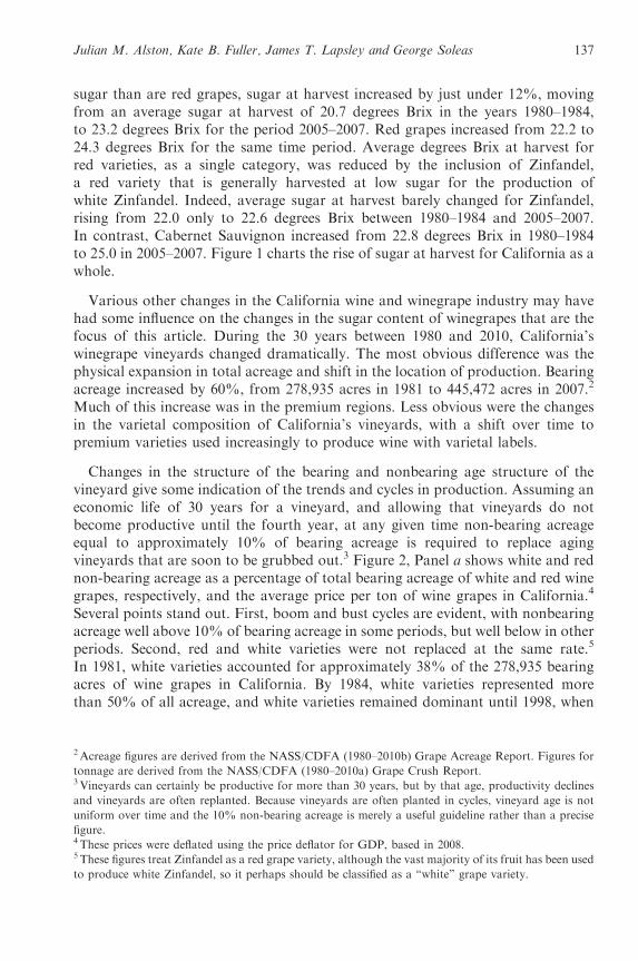
sugar than are red grapes, sugar at harvest increased by just under 12%, movingfrom an average sugar at harvest of 20.7 degrees Brix in the years 1980–1984,to 23.2 degrees Brix for the period 2005–2007. Red grapes increased from 22.2 to24.3 degrees Brix for the same time period. Average degrees Brix at harvest forred varieties, as a single category, was reduced by the inclusion of Zinfandel,a red variety that is generally harvested at low sugar for the production ofwhite Zinfandel. Indeed, average sugar at harvest barely changed for Zinfandel,rising from 22.0 only to 22.6 degrees Brix between 1980–1984 and 2005–2007.In contrast, Cabernet Sauvignon increased from 22.8 degrees Brix in 1980–1984to 25.0 in 2005–2007. Figure 1 charts the rise of sugar at harvest for California as awhole.

Various other changes in the California wine and winegrape industry may havehad some influence on the changes in the sugar content of winegrapes that are thefocus of this article. During the 30 years between 1980 and 2010, California’swinegrape vineyards changed dramatically. The most obvious difference was thephysical expansion in total acreage and shift in the location of production. Bearingacreage increased by 60%, from 278,935 acres in 1981 to 445,472 acres in 2007.2

Much of this increase was in the premium regions. Less obvious were the changesin the varietal composition of California’s vineyards, with a shift over time topremium varieties used increasingly to produce wine with varietal labels.

Changes in the structure of the bearing and nonbearing age structure of thevineyard give some indication of the trends and cycles in production. Assuming aneconomic life of 30 years for a vineyard, and allowing that vineyards do notbecome productive until the fourth year, at any given time non-bearing acreageequal to approximately 10% of bearing acreage is required to replace agingvineyards that are soon to be grubbed out.3 Figure 2, Panel a shows white and rednon-bearing acreage as a percentage of total bearing acreage of white and red winegrapes, respectively, and the average price per ton of wine grapes in California.4

Several points stand out. First, boom and bust cycles are evident, with nonbearingacreage well above 10% of bearing acreage in some periods, but well below in otherperiods. Second, red and white varieties were not replaced at the same rate.5

In 1981, white varieties accounted for approximately 38% of the 278,935 bearingacres of wine grapes in California. By 1984, white varieties represented morethan 50% of all acreage, and white varieties remained dominant until 1998, when

2Acreage figures are derived from the NASS/CDFA (1980–2010b) Grape Acreage Report. Figures for

tonnage are derived from the NASS/CDFA (1980–2010a) Grape Crush Report.3 Vineyards can certainly be productive for more than 30 years, but by that age, productivity declines

and vineyards are often replanted. Because vineyards are often planted in cycles, vineyard age is not

uniform over time and the 10% non-bearing acreage is merely a useful guideline rather than a precise

figure.4 These prices were deflated using the price deflator for GDP, based in 2008.5 These figures treat Zinfandel as a red grape variety, although the vast majority of its fruit has been used

to produce white Zinfandel, so it perhaps should be classified as a “white” grape variety.

Julian M. Alston, Kate B. Fuller, James T. Lapsley and George Soleas 137

red varieties accounted for 50.7%. The trend toward red varieties has continuedand in 2007 red varieties claimed just under 62% of all California winegrapeacreage.

Figure 1

Trends in Sugar Content (Degrees Brix) of California Wine Grapes,

1980–2008

1980 1985 1990 1995 2000 200519

20

21

22

23

24

25

Average Degrees Brix for Total Red Wine Grapes, State Total

(Average annual percent change: 0.23%)

1980 1985 1990 1995 2000 200519

20

21

22

23

24

25

Average Degrees Brix for Total White Wine Grapes, State Total


1980 1985 1990 1995 2000 200519

20

21

22

23

24

25

Average Degrees Brix for Total Wine Grapes, State Total


Source: Created by the authors using data from NASS/CDFA Grape Crush Reports,1981–2010.


The state aggregate figures mask significant spatial variation. As can be seen inFigure 2, Panel b, in most years during the two decades from 1985 to 2005, Napaand Sonoma counties had a higher percentage of non-bearing acreage than did thestate as a whole. These counties suffered a phylloxera infestation in the 1980s and1990s, necessitating replanting of existing vineyards as well as new vineyardplantings to meet increased demand. During this period, wine consumers in theUnited States increasingly chose varietally labeled wine, leading to the dominanceof “premium” varieties such as Chardonnay, Cabernet Sauvignon, Zinfandel, andMerlot. In 1985, only 19% of California table wine carried a varietal label, but

Figure 2

Nonbearing Acreage of Wine grapes as a Percentage of Bearing Acreage

Panel b:

Panel a:

0

200

400

600

800

1000

0

5

10

15

20

25

1981 1986 1991 1996 2001 2006

Red White Avg $/ton

% Nonbearing 2008 $

0

5

10

15

20

25

30

35

40

1981 1986 1991 1996 2001 2006

Napa/Sonoma Statewide

% Nonbearing

Source: Created by the authors using data from NASS/CDFA Grape Acreage Reports,

1982–2010.


within 15 years, by 2000, varietally labeled wine accounted for 71% of allCalifornia table wine by volume (Shanken, 2001, p. 97).6 Although costly inmaterials and lost harvest revenue, the replanting in Napa and Sonoma roughlycoincided with a market swing to red wine in the 1990s, and allowed vineyardowners to convert their vineyards to red varieties, especially Cabernet Sauvignonand Merlot, while adopting higher planting densities and new trellising systems.

The trend to grow premium varieties of red wine was accompanied by a shiftto produce a greater share of production in the premium regions. In 1981 slightlymore than 50% of California’s winegrape acreage was located in the southernSan Joaquin Valley but by 2008, this percentage had fallen to slightly more than33% of acreage. While total California winegrape vineyard acreage had expandedby 164,756 acres (a 59% increase), San Joaquin Valley acreage had increased byonly 12,422 acres, or 8.5%. As can be seen in Figure 3, the areas experiencing thegreatest percentage growth in acreage were the Delta, which grew by 185% from17,355 acres in 1981 to 49,558 acres in 2008; the North Coast, which expanded by128% from 55,474 acres in 1981 to 87,726 acres in 2008; and the Central Coast,which doubled in size from 41,015 acres in 1981 to 82,600 acres in 2008.7

California’s vineyard regions differ significantly in yield and in perceived quality,which is reflected in the average price per ton paid for grapes from differentregions. Figure 4 shows the average price per ton for Cabernet Sauvignon andChardonnay wine grapes for five California viticultural areas in 2008. The priceranged from an average price of $4,648 a ton for Cabernet Sauvignon grown inNapa County, to a low of $363 a ton for the same variety grown in district 14,which is located at the southern end of the San Joaquin Valley. The higherprices paid for Cabernet from Napa and Sonoma counties reflect the veryreal compositional differences, such as higher acidity, deeper color, and greaterintensity, relative to grapes grown in California’s warm interior valley. To someextent the prices also are indicative of yield. In 2008, Napa County vineyardsdelivered 2.4 tons of Cabernet per acre, and neighboring Sonoma County yieldswere only a bit higher at 2.8 tons. In the warm interior valley, Delta vineyardsproduced 7.6 tons per acre of Cabernet while district 14 yielded 15.1 tons per acre.Monterey and San Benito counties in California’s Central Coast, yielded 4.4 tonsper acre.

6Under U.S. law, varietally labeled wine must contain at least 75% of the named variety.7 For the present purpose, we have divided California into five viticultural areas: (1) the “North Coast,”

including Napa, Sonoma, Mendocino, Lake and Marin counties; (2) the “Central Coast,” including

Monterey, San Benito, San Luis Obispo, and Santa Barbara counties; (3) the “Delta,” which includes

the northern portion of San Joaquin County and southern portions of Yolo and Sacramento counties

adjacent to California’s delta; (4) the “San Joaquin Valley,” comprising southern San Joaquin County,

Stanislaus, Merced, Madera, Fresno, Tulare, Kings and Kern counties; and “Other” which includes the

Sierra foothills, southern California, and the northern Sacramento Valley (in aggregate the “Other” area

comprises approximately 6% of vineyard acreage and 3.5% of total tonnage).


In Figure 5, Panel a shows the percentage of tons by region while Panel bdisplays the percentage of value by region in 2008. The North Coast, whichaccounted for just less than 10% of all grapes crushed, commanded over 38% of allrevenue. It is followed by the Central Coast, which grew 9.4% of all tons crushedand claimed 18.8% of revenue. The Delta, the coolest area of California’s interiorvalley, delivered 17.1% of all grapes crushed, and received 13.5% of the revenue.

Figure 3

Regional Distribution of California Winegrape Acreage, 1981 and 2008

0

20

40

60

80

100

120

140

160

180

North Coast Central Coast Delta SJV Other

Acr

es (

1000

's)

Source: Created by the authors using data from NASS/CDFA Grape Acreage Reports,1982–2010.


The southern San Joaquin Valley, responsible for producing 61% of California’sharvest, received just under 27% of the revenue. Clearly growing grapes is asignificantly different business in Napa than in the San Joaquin Valley.

III. A Simple Model of Determinants of Sugar in Wine Grapes

It is unclear why sugar has increased at harvest but several contributing factorshave been suggested. Global warming is often mentioned. For instance, averageminimum temperatures in the San Joaquin Valley rose by about 2.5 degreesFahrenheit (almost 1.4 �C) from the 1930s to the first years of the 21st century,and most of that increase became apparent during the most recent 20–30 years(Bar-Am, 2012, in process; see also Weare, 2009). Denser coastal vineyardplantings and new trellising systems are also often cited. Some wine makers pointto the new rootstock/scion interactions that were introduced following the collapseof the rootstock, AXR to phylloxera, indicating that these new vineyards achievesugar ripeness prior to reaching phenolic maturity, making it necessary for thegrapes to “hang” longer than in the past. Still others claim that higher sugar atharvest is simply a style choice, with no underlying physiological reason to befound in the vineyard.

Whatever, the case, it is clear that higher sugar grapes, if fermented to dryness,result in higher alcohol wines. Higher alcohol in wines may or may not be a desiredoutcome. The presence of more alcohol can contribute to a perception of “hotness”for some consumers, while for others higher alcohol may add a sense of sweetnessto the wine. However, under the United States tax system, wines above 14%alcohol by volume are taxed at $0.50 a gallon more than are wines with less than

Figure 4

Price of Cabernet Sauvignon and Chardonnay in Various Places, 2008

0

1000

2000

3000

4000

5000

6000

Napa Sonoma Monterey

in $/ton

Delta Kern

Cabernet Sauvignon Chardonnay



14% alcohol by volume.8 The demand to reduce alcohol concentrations has givenrise to a new business in California, alcohol reduction. Currently two firms, WineSecrets and ConeTech, specialize in alcohol removal. Use of such technologyindicates a demand to reduce the alcohol content of wine.9

Figure 5

Total Tons Harvested and Value in 1980 and 2008, by Region

0

5

10

15

20

25

30

35

80020891

Ton

s (i

n 10

0,00

0's)

North Coast Central Coast Delta San Joaquin Valley Other

0

500

1000

1500

2000

2500

80020891

$ (M

illio

ns)

North Coast Central Coast Delta San Joaquin Valley Other


8 Federal tax rates are $1.07 per gallon for wine having 7 to 14% alcohol and $1.57 per gallon for wine

between 14 and 21% alcohol by volume. See http://www.ttb.gov/tax_audit/atftaxes.shtml9 Based on its production of “proof gallons,” we estimate that ConeTech alone treated roughly 3.3

million gallons of wine per year for the four years 2005–2008, which represents a finished amount of

approximately 16.5 million gallons (assuming 20% of a lot would be treated), or about 3% of

California’s annual wine production. ConeTech indicates that they have sold their technology to several

large California wineries, but declined to name their clients.


In this section we develop a model of winegrape production and quality,including sugar content and other characteristics as choice variables alongwith yield, which we can use to derive hypotheses about alternative theoreticalexplanations for the phenomenon of rising sugar content of grapes. Growers’variable profit per acre of wine grapes of variety v grown in crush district d in year tis equal to gross revenue per acre (yield in tons per acre, Yvdt times the price perton, Pvdt) minus variable costs (the quantity of variable inputs used per acre, Xvdt

times the price per unit of inputs, vt). That is:

p Gdvt ¼ PdvtYdvt � vtXdvt: ð1Þ

The price of wine grapes varies, depending on their sugar content, B (in degreesBrix) and other physical quality characteristics, Q (such as acidity), as well as thevariety, V, the district, D, and the year, Y (reflecting market conditions). Thus:

Pdvt ¼ p Bdvt;Qdvt;Dd;Vv; Ttð Þ: ð2Þ

The yield of wine grapes varies among crush districts, varieties, and years, and withchanges in the quantity of variable inputs, X; it also depends on weather conditionsduring the growing season in the crush district, Wdt (a complex of rainfall andtemperature variables), and management practices applied to the particular variety,Mdvt. The yield relationship may also vary over time reflecting year-to-yearand secular changes in technology that are not captured in the weather andmanagement variables (e.g., because of changes in climate, rootstocks, pest anddisease prevalence, or other factors), and the variable Tt is included to representthese aspects.

Ydvt ¼ p Xdvt;Wdt;Mdvt;Dd;Vv; Ttð Þ: ð3Þ

The sugar content of wine grapes (B) and other quality characteristics (Q) dependon the same factors that affect yield.

Bdvt ¼ b Xdvt;Wdt;Mdvt;Dd;Vv; Ttð Þ: ð4Þ

Qdvt ¼ q Xdvt;Wdt;Mdvt;Dd;Vv; Ttð Þ: ð5Þ

Winemakers’ variable profit per gallon of bulk wine (or equivalent quantity ofwine grapes) produced using variety v grown in crush district d in year t is equal togross revenue per gallon, Gdvt minus (a) the cost of excise taxes per gallon, E, whichdepend on the alcohol content of the wine, Advt, (b) the cost of the wine grapes,(c) variable costs of winemaking (the quantity of variable inputs used per gallon,Zvdt times the price per unit of inputs, rt), and (d) expenditure on removal ofalcohol from wine, Svdt.

10 That is:

pWdvt ¼ Gdvt � EðAdvÞ � PdvtYdvt � rtZdvt � Sdvt: ð6Þ

10 It might be useful to disaggregate into several categories of winemaking inputs for some purposes but

for now we treat Z as a scalar aggregate, as we did with X for grape production.


The value of wine per gallon depends on its alcohol content, A, other physicalquality characteristics, K, as well as the variety, V, the district, D, and the year, Y.

Gdvt ¼ g Advt;Kdvt;Dd;Vv; Ttð Þ: ð7Þ

The alcohol content of the wine depends on the sugar content of the wine grapes,but can be modified by the expenditure of effort, S.

Advt ¼ a Bdvt; Sdvtð Þ: ð8Þ

Other quality characteristics of the wine depend on the same variables, as well asthe quality characteristics of the wine grapes, Q, the quantity of winemakinginputs, Z, and oenological management practices in the winery, O.

Kdvt ¼ k Qdvt;Odvt;Bdvt; Sdvt;Advt;Dd;Vv; Ttð Þ: ð9Þ

We draw informally on this model in proposing two hypotheses about the sourcesof the rise in sugar content of California winegrapes. In each case the increasein sugar content of grapes is seen as an unsought consequence of other factors.The first hypothesis is that exogenous changes in the weather, with generally risingaverage temperatures, imply increases in sugar content of grapes even without anychanges in management of the vineyard.11 Profit-maximizing responses of growersand wineries to such changes could mitigate the implications for sugar content ofgrapes but should not be expected entirely to eliminate their impact.

The second hypothesis is that the trend was caused by a market demand(perceived or real) for wines with ripe flavors and lower tannin levels, attributesassociated with grapes that are picked at higher degrees Brix. Under thishypothesis, profit-maximizing responses of wineries and growers to changes indemand for quality characteristics of wine required changes in viticultural practicesthat resulted in unsought increases in sugar content of grapes. For instance,extending the “hang time” and picking the grapes later than they would dootherwise is likely to result in higher sugar content, if only because the grapes aremore dehydrated.12 To some extent vignerons can independently manage the sugar

11A literature is developing on the implications of climate and climate change for the wine industry, and

some of that specific to California. Examples include Nemani et al. (2001), Tate (2001), Jones (2005,

2006, 2007), Jones et al. (2005), Webb et al. (2005), White et al. (2006), and Jones and Goodrich (2008).

Issues addressed include various aspects of wine quality, yield, and the optimal location of production.

Published work to date has not quantified the impacts on sugar content of grapes that are the subject of

our work.12More-specifically, influential wine writers, such as Robert Parker of the Wine Advocate or James

Laube of the Wine Spectator, may have encouraged the production of wines with strong, intense, riper

fruit flavors, by giving very favorable ratings for such wines. This argument applies more directly to

ultra-premium wines than to the large volume end of the market that is not subject to wine ratings, and

probably more to red wines than white wines. However, changes in the ultra-premium end of the market

might have led to similar subsequent movements in wines in the lower price categories. In addition,

some of the market growth of moderately priced wines might have been facilitated by an emphasis on

similar styles of wine that are attractive to less experienced wine consumers.


content of grapes and other quality characteristics, but an increase in intensity andripeness of fruit is likely to come to some extent at the expense of a reduction intons per hectare and an increase in degrees Brix.13

IV. Changing Sugar Content of California Wine Grapes

We assembled a very detailed data set (from annual crush reports and various othersources) that includes (a) annual data by variety of grapes and crush district on theaverage sugar content of wine grapes at crush, extending from 1980 through 2008,(b) other data on yield, acreage, and production of wine grapes by variety andcounty, and (c) daily data on temperatures by crush district. Using these data, weestimated variants of the following model to examine the extent of changes indegrees Brix (BRIX) over time among crush districts and varieties and the role ofclimate as represented by a heat index:

BRIXdvt ¼ b0 þ bhHdt þ �V

j¼1n jVARvj þ �

D

i¼1d dDISTdi þ t 0Tt þ �

V

j¼1t v

j VARvjrTt

� �

þ �D

i¼1t d

i DISTdirTtð Þ þ edvt ð10Þ

In this model, Hdt is a weather variable, the “heat index” for crush district d duringthe growing season in year t. The other variables are dichotomous dummy (orindicator) variables such that VARvj = 1 if j = v, 0 otherwise, and DISTdi = 1 if i = d,0 otherwise), and a time trend, Tt.

A. Definitions of Variables and Data for the Analysis

We have data for the years 1980–2008 on average degrees Brix for over 200varieties in 17 crush districts. (The number of varieties reported changes from yearto year and from district to district. Varieties include wine, table, and raisingrapes.)14 Table 1 reports average annual growth rates over the longer period1980–2008 as well as 1990–2008, for a selection of important varieties, as well as forall red, all white, and all varieties, in each of the main production regions and forCalifornia as a whole. The data in the table are suggestive of the possibility thatgrowth rates may have differed systematically among regions and varieties, an issuethat we examine next. The statistical analysis that follows uses only the data for the

13A literature on the economic effects of weather and climate on wine quality has developed over the

past 20 years, with contributions such as Ashenfelter, Ashmore and Lalonde (1995), Ashenfelter and

Byron (1995), Jones et al. (2005), Storchmann (2005), Ashenfelter (2008), and Ashenfelter and

Storchmann (2010).14 These data were compiled from the Annual Grape Crush Reports, published by NASS/CDFA,

various issues.


more recent period, 1990–2008, for which the data are more consistent and morecomplete, and the estimated relationships are more likely to be stable andmeaningful.

Table 1Trends in Sugar Content of California Wine Grapes (Degrees Brix), by Variety and Region

(a) 1980–2008

Variety

Region

NorthCoast

CentralCoast Delta

San JoaquinValley

SouthernCalifornia California

average annual percentage change

Sauvignon Blanc - 0.02 0.11 0.05 0.51 0.20 0.16

French Colombard - 0.12 – 0.25 0.22 – 0.20

Chardonnay 0.18 0.32 0.29 0.37 0.19 0.18

Chenin Blanc 0.05 0.29 0.30 0.33 - 0.11 0.29

All White Varieties 0.30 0.42 0.68 0.40 0.61 0.47

Cabernet Sauvignon 0.30 0.25 0.33 0.23 0.38 0.25

Merlot 0.15 0.32 0.38 0.10 – 0.19

Zinfandel 0.37 0.17 0.07 - 0.29 0.07 - 0.16

Pinot Noir 0.39 0.30 – 0.72 – 0.42

All Red Varieties 0.36 0.35 0.27 0.17 0.18 0.26

All Varieties 0.34 0.38 0.34 0.22 0.30 0.31

(b) 1990–2008

Variety

Region

NorthCoast

CentralCoast Delta

San JoaquinValley

SouthernCalifornia California

average annual percentage change

Sauvignon Blanc 0.18 0.39 0.08 0.37 0.42 0.21

French Colombard - 0.05 – 0.19 0.04 – 0.04

Chardonnay 0.35 0.49 0.39 0.22 0.00 0.32

Chenin Blanc 0.12 0.72 0.23 0.16 0.07 0.20

All White Varieties 0.36 0.63 0.69 0.26 0.25 0.43

Cabernet Sauvignon 0.50 0.49 0.46 0.29 0.53 0.42

Merlot 0.44 0.55 0.44 0.18 0.35 0.40

Zinfandel 1.11 1.01 1.02 0.33 0.60 0.55

Pinot Noir 0.88 0.63 0.75 1.49 0.26 0.87

All Red Varieties 0.72 0.75 0.96 0.31 0.49 0.53

All Varieties 0.57 0.69 0.85 0.36 0.43 0.53

Notes. Entries in this table are average annual percentage changes, computed as ln(final value) – ln(initial value) divided by the number of

years and multiplied by 100. For some years and some varieties, records are unavailable. In the table, this is indicated by “—.”

Source: Created by the authors using data from NASS/CDFA Grape Crush Reports, 1981–2010.


The daily measure of growing degrees (GDs) is equal to the average of the dailyminimum and daily maximum temperature minus a base temperature of 50�F.The growing season for wine grapes is defined as extending over the six months,April through September. The accumulated total of growing degree units (GDUs)is the sum of GDs accumulated during the season. We use a growing seasonheat index, H defined as the average daily GDs during the growing season, equalto the accumulated GDUs divided by the total number of days.15 We alsoexperimented with the same variable applied to different periods (e.g., the entireyear or particular months).

The data on monthly temperature averages were obtained from NOAA’sNational Climatic Data Center (NOAA, 2010). From hundreds of NOAA stationswithin California, we chose one weather station for each of the 17 crush districts.While more localized data would have been preferred, none were available.However, Lecocq and Visser (2006) showed that while highly localized data makefor better-fitting models, weather station data approximate the disaggregated dataquite well (see, also, Haeger and Storchmann, 2006). We attempted to find stationsthat were geographically central to wine-growing areas within each district, whilemaking sure that the station locations were not at higher altitudes, or wereotherwise different from the areas where winegrapes are grown. In some instances,it was difficult to find a well-located station for which data were available foreach month in the entire span of time we are examining. Some stations arerelatively new, and so do not have historical data reaching more than several yearsback. Other stations have been shut down or have large gaps in reporting. As aresult, we used some data from stations that were not ideal for our purposes, andwe used the same weather station for districts 11 and 12.16 Faced with a similar

15We thank Professor Andrew Walker from the Department of Viticulture and Enology at UC Davis

for advising us about the appropriate choice of a heat index for our purpose.16We were able to obtain data from the NOAA website for a number of weather stations in the Napa

Valley on monthly average temperatures for the years 1990 through 2007, that we could use to compute

our growing season heat index. None of these stations is located in the center of the vineyard area in the

Napa Valley, and away from urban and other influences, as would be ideal for the purpose.

Temperatures vary significantly within the valley, tending to increase as you go North and East, and

consequently particular locations may not be fully representative of the Valley as a whole. In our initial

analysis we used data from Markley Cove, which is at a higher altitude on the Eastern edge of Napa

County, and somewhat warmer than locations in the Valley floor, especially at the Southern end. Data

from Napa City Hospital, at the Southern end of the Valley, reflect a combination of urban influence

and generally cooler conditions. Data from Healdsburg, which we used for Sonoma county, are more

likely to be representative of the Napa Valley as a whole, because Healdsburg has temperature patterns

quite similar to those of St Helena, which is somewhat warmer than the city of Napa, at the Southern

end of the Valley. When we tried using data for Healdsburg instead of Markley Cove, the results were

essentially identical. Based on this analysis we concluded that the results were not sensitive to the choice,

and we report the results we obtained in the first instance, using data from Markley Cover to represent

the Napa crush district.


problem, Storchmann (2005) regressed Rhine wine quality on English weatherfrom 1700–2003.

We tried the model in equation (11) with different aggregations of varietiesand districts in preliminary analysis. To reduce the dimensions of the problem ofreporting and interpreting results we opted to aggregate crush districts into fourlarger regions based on the average price of wine grapes in 2008. Table 2 showsthe districts as classified. Similarly, rather than model individually every winegrapevariety we included various aggregates such as “red” versus “white,” and“premium” versus “non-premium” varieties, where “premium” included CabernetSauvignon, Merlot, and Chardonnay (we tried including Pinot Noir as well, but theresults were not affected much).

B. Regression Results for Model of Changes in Brix in California,1990–2008

Each of the four columns in Table 3 refers to a different variant of the model inequation (12). We estimated each model by ordinary least squares (OLS) but wherepossible we used Newey-West robust standard errors for hypothesis testing ratherthan the conventional OLS robust standard errors. We also ran the model withcluster-robust standard errors, but the effect on the results was very small. As wellas estimating each model using conventional OLS we also estimated each modelusing weighted regression, where the data from each crush district were weighted

Table 2Definitions of Regions

Region (average winegrape price in 2008) Includes Crush Districts

Ultra-premium (>$2,000/ton) 3 (Sonoma)

4 (Napa)

Premium ($1,000 – $2,000/ton) 1 (Mendocino)

2 (Lake)

6 (San Francisco area)

7 (Monterey, San Benito)

8 (Santa Barbara area)

10 (Sierra Foothills area)

15 (Los Angeles, San Bernardino)

16 (San Diego area)

Fine ($500 – $1,000/ton) 5 (Solano)

9 (Northern California area)

11 (San Joaquin, part of Sacramento)

17 (parts of Yolo, Sacramento)

Ordinary (< $500/ton) 12 (Merced area)

13 (Fresno area)

14 (Kern, parts of Kings, Tulare)


Table 3Brix Regression Results, Annual Observations 1990–2008

a: Weighted Observations

Regressor (1) (2) (3) (4)

Constant 20.91** 18.79** 19.25** 0.58**

(0.107) (0.447) (0.418) (0.424)

[0.187] [0.649] [0.616]

Trend 0.14** 0.10** 0.02 0.01**

(0.011) (0.009) (0.011) (0.007)

[0.020] [0.015] [0.018]

Variety

Red 0.96** 0.22 0.19**

(0.087) (0.158) (0.091)

[0.156] [0.274]

Premium 1.89** 2.25** 0.36**

(0.072) (0.119) (0.100)

[0.123] [0.200]

Region

Ultra-premium 1.34** 0.48 0.40**

(0.121) (0.176) (0.116)

[0.189] [0.290]

Premium 1.71** 0.80* 0.50**

(0.206) (0.215) (0.140)

[0.302] [0.336]

Fine 0.28 - 0.91* 0.18**

(0.137) (0.265) (0.154)

[0.241] [0.463]

Heat Index (Growing Season Average Degree Days) 0.04* 0.05* 0.03**

(0.018) (0.017) (0.010)

[0.027] [0.025]

TrendrRegion

Ultra-Premium 0.09** - 0.01

(0.014) (0.009)

[0.023]

Premium 0.09** - 0.00

(0.013) (0.009)

[0.021]

Fine 0.10** 0.00

(0.023) (0.013)

[0.040]

TrendrVariety

Red 0.08** 0.00

(0.005) (0.008)

[0.025]

Premium - 0.03** - 0.02**

(0.0051) (0.008)

[0.019]

Brix(Year-1)

0.35**

(0.030)

Brix(Year-2)

0.41**

(0.029)

Brix(Year-3)

0.17**

(0.033)

Adjusted R2 0.14 0.49 0.52 0.91

RMSE 1.94 1.49 1.45 0.63


b: Unweighted Observations

Regressor (1) (2) (3) (4)

Constant 21.87** 19.97** 20.35** 3.69**

(0.032) (0.121) (0.140) (0.371)

[0.049] [0.173] [0.206]

Trend 0.14** 0.13** 0.09** 0.03**

(0.003) (0.003) (0.008) (0.007)

[0.004] [0.004] [0.013]

Variety

Red 1.05** 0.77** 0.21**

(0.031) (0.063) (0.078)

[0.048] [0.093]

Premium 0.70** 0.90** 0.18**

(0.026) (0.049) (0.059)

[0.039] [0.072]

Region

Ultra-premium 1.28** 1.00** 0.50**

(0.060) (0.117) (0.127)

[0.091] [0.174]

Premium 1.25** 0.97** 0.58**

(0.057) (0.091) (0.088)

[0.085] [0.139]

Fine 0.74** 0.38* 0.41**

(0.057) (0.107) (0.104)

[0.090) [0.166]

Heat Index (Growing Season Average Degree Days) 0.02** 0.02** 0.02**

(0.005) (0.005) (0.004)

[0.006] [0.006]

TrendrRegion

Ultra-Premium 0.03 - 0.01

(0.010) (0.010)

[0.015]

Premium 0.03* - 0.01

(0.008) (0.007)

[0.012]

Fine 0.03* - 0.01

(0.010) (0.009)

[0.015]

TrendrVariety

Red 0.03** 0.01

(0.006) (0.006)

[0.008]

Premium

- 0.02** - 0.00

(0.005) (0.005)

[0.006]

Brix(Year-1)

0.35**

(0.032)

Brix(Year-2)

0.28**

(0.036)

Brix(Year-3) 0.17**

(0.020)

Adjusted R2 0.14 0.26 0.27 0.61

RMSE 1.83 1.69 1.68 1.20

OLS robust standard error in parentheses. Newey-West robust standard error in square brackets. **, * Significant at the 1% and 5% levels,

respectively, using Newey-West except in column (4). 13,379 observations.


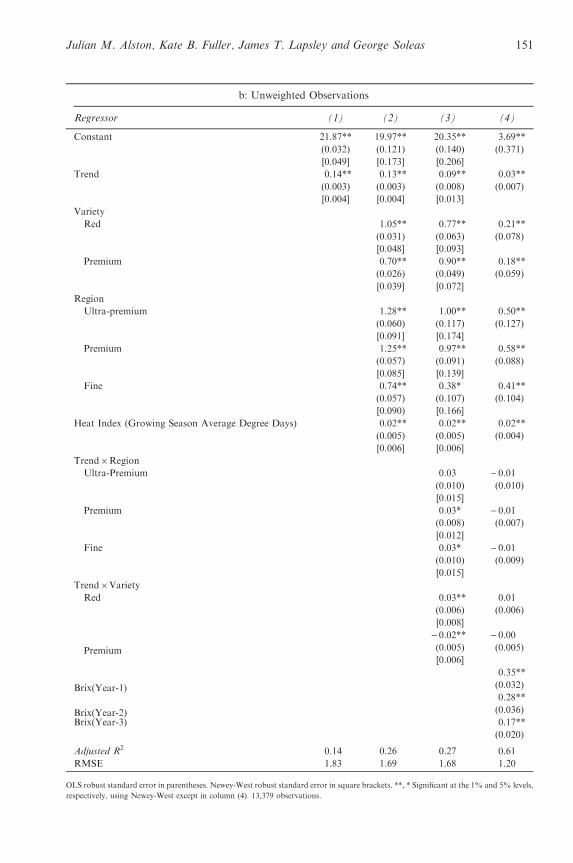
according to shares of California’s total production.17 The rationale for using aweighted regression is that the data we are using are themselves annual averages forparticular varieties within individual crush districts, with very different numbers ofobservations contributing to the average, depending on the volume of the crush.We prefer the estimates from the model using weighted regression, as reported inPanel a of Table 3. The results from the same models using the unweighted data arealso presented for comparison in Panel b of Table 3.

In Table 3, Panel a, column (1) includes the results from a regression of Brixagainst trend for all varieties and regions. The model predicts that on average,sugar content of California wine grapes increased by 0.14 degrees Brix per yearover the years 1990–2008 from a base of 21.7 in 1989, a predicted increase of2.5 degrees Brix, or 11.6 percent over the period. In column (2) the model isaugmented with a weather variable (the heat index for the growing season), andvarious dummy variables for Variety and Region, retaining the assumption of asingle trend growth rate applying to all varieties and regions. The trend growth ratein this model is slightly lower, 0.10 rather than 0.14 degrees Brix per year.

The coefficient on the heat index is positive and statistically significant indicatingthat a 1 degree increase in the index would result in a 0.04 degrees Brix increase inthe sugar content of wine grapes. This is a comparatively small effect, since a1 degree increase in the heat index requires a large temperature increase.18 The firstVariety dummy is set equal to 1 for “red” varieties (including Zinfandel, althoughsignificant quantities of Zinfandel are used to make White Zinfandel). The secondVariety dummy is set equal to 1 for “premium” varieties (Cabernet Sauvignon,Merlot, or Chardonnay). Regional dummies represent the “fine,” “premium,” and“ultra premium” regions as defined in Table 2 such that the default region is“ordinary.” The coefficients on all of the dummy variables for Varieties andRegions are positive and statistically significant (with the marginal exception of the“fine” region), indicating that red varieties, and premium varieties, and grapes fromdistricts commanding price premia could be expected to have higher sugar contentat crush compared with the default category.

In this case we interpret the intercept (18.79) as applying to the default categoryof “non-premium,” “white” varieties from the “ordinary” region (crush districts12, 13, and 14 in the southern San Joaquin Valley). The counterpart for redvarieties is higher by 0.96 degrees Brix, the estimated dummy variable coefficient,and the counterpart for premium varieties is higher by 1.89 degrees Brix. It can beseen that compared with the default region (“ordinary”) the other regions have

17 The weights were calculated using STATA’s “aweight” option, with the weights for particular

observations equal to the corresponding observation-specific tons crushed as a share of total California

tonnage in the same year.18 For instance, an increase by 1 degree Fahrenheit in both the average daily minimum and the average

daily maximum temperature throughout the six-month growing period would imply 1 degree increase in

the index.


higher degrees Brix associated with higher prices for wine grapes: by 0.28 degreesBrix for the “fine” region, 1.71 degrees Brix for the “premium” region and 1.34degrees Brix for the “ultra premium” region. These results are consistent with theidea that higher sugar content and higher alcohol content are less desirable inlower-priced wine grapes, possibly because of the additional $0.50 cents per gallontax on wine with more than 14 percent alcohol by volume.

The model in column (3) augments the model in column (2) with variables thatinteract the time trend with the dummy variables for varieties and regions. In thismodel the coefficient on the heat index indicates that a 1 degree increase in theindex would result in a 0.05 degrees Brix increase in the sugar content of winegrapes, slightly higher than that in the model without interaction terms, but thecoefficient on the time trend (the growth rate for the default category) and severalof the coefficients on the dummy variables for Varieties and Regions are no longerstatistically significant. Still, premium varieties (but no longer red varieties) andgrapes from the premium and fine districts (but not the ultra-premium district)could be expected to have higher sugar content at crush compared with the defaultcategory.

The interaction terms indicate significantly faster growth rates in sugar contentfor red varieties and premium varieties, and for grapes from the premium and fineregions, compared with the default; they indicate a slower growth rate for the ultra-premium region. The coefficients on the interaction terms represent the additionalgrowth in degrees Brix per year for the dummy category relative to the default. Thedefault category is non-premium, white varieties in the ordinary wine region, forwhich the trend growth rate is 0.02 degrees Brix per year from a base of 19.25degrees Brix. Thus, for instance, for a premium white variety in the premiumregion, the corresponding estimate is a trend growth rate of 0.14 (0.02+0.09+0.03)degrees Brix per year from a base of 22.30 (19.25+2.25+ 0.80) degrees Brix.

Column (4) of Table 3 represents the same model as in column (3) augmentedwith lagged values of the dependent variable. We experimented with the number oflags of the dependent variable to include. The adjusted R-squared is maximizedand the Akaike Information Criterion (AIC) is minimized when three lags areincluded, so that is the model we are reporting. In models with lagged dependentvariables we could not compute Newey-West measures and so we report the OLSrobust standard errors. Notably the coefficients on all three lagged-dependentvariables are individually statistically significant, and diminishing with lag length,and they sum to 0.93, which means that in this model shocks have very persistenteffects on the dependent variable. In addition, the long-run impact of a shock is onthe order of 10–20 times its initial impact.19 This implication of the model mightnot be equally plausible for all types of shocks. Otherwise, this model is to be

19 The long-run multiplier for a permanent increase is equal to the short-run multiplier, divided by one

minus the sum of the coefficients on the lagged dependent variable: 1/(1–0.93) = 14.3.


preferred, on grounds of its superior statistical performance, to the one in column(3) that omits the lagged values of the dependent variable.

The coefficients for this model are generally plausible, and they are largelyconsistent with those of the variant in column (3). The coefficient on the heat indexindicates that a 1 degree increase in the average heat index would result in a 0.03degrees Brix increase in the sugar content of wine grapes in the current year.Taking the lagged dependent variables into account, a permanent increase in theheat index by 1 degree Fahrenheit would imply a 0.43 degrees Brix increase in thesugar content of wine grapes in the ultimate long run. Compared with the defaultvariety, non-premium white, for red varieties sugar content is higher by 0.19degrees Brix and for premium varieties it is higher by 0.36 degrees Brix. As in theother models, compared with the default region (“ordinary”) the other regions havehigher degrees Brix associated with higher prices for wine grapes: by 0.18 degreesBrix for the “fine” region, 0.50 degrees Brix for the “premium” region and 0.40degrees Brix for the “ultra premium” region. Importantly, none of the coefficientson interactions of trend with region, or trend with red varieties, is statisticallysignificant. For these categories the coefficient on the trend is the same as for thedefault category, 0.01 degrees Brix per year. Only for premium varieties is the trendgrowth rate significantly different: it is lower by 0.02 degrees Brix per year.

Table 4Trends in the Heat Index by Crush District and for California, 1990–2008

Crush DistrictAnnualized Average

Change (%)100*Slope from Regression

of Ln(Heat) on Trend

percent per year

1 - 0.30 - 0.23 (0.357)

2 - 0.18 0.11 (0.722)

3 0.58 0.75 (0.007)

4 0.01 0.20 (0.374)

5 0.03 - 0.01 (0.979)

6 - 0.50 - 0.16 (0.600)

7 - 0.69 - 0.55 (0.271)

8 - 0.60 - 0.05 (0.919)

9 0.02 0.14 (0.445)

10 0.85 1.01 (0.004)

11 - 0.19 - 0.09 (0.725)

12 - 0.19 - 0.09 (0.725)

13 0.22 0.25 (0.224)

14 0.22 0.26 (0.312)

15 0.04 0.27 (0.249)

16 - 0.31 - 0.83 (0.033)

17 0.07 0.28 (0.195)

State Average (Weighted) 0.06 0.12 (0.405)

Notes: The weather station is the same for Districts 11 and 12. The annual heat index is a weighted average across crush districts, where the

weights are tons crushed in the respective districts as a share of the total California tonnage. Standard errors in parentheses.


Of particular interest here is the relative importance of the heat index as anexplanation of the rise in Brix. Across all the models, the results suggest that even asubstantial rise in average temperature (or the average of the daily maximum andminimum temperatures) during the growing season would have had only modesteffects on the sugar content of wine grapes. In fact, however, our data do not showa substantial rise in temperature between 1990 and 2007, as measured by the heatindex. Table 4 includes two measures of the average trend rate in the index for eachcrush district: (a) the simple average of the annual proportional growth rates asmeasured by the logarithmic difference, and (b) the trend growth rate, from aregression of the logarithm of the index against a time trend. The estimates areexpressed as annual percentage growth rates, and they include a mixture of smallpositive and negative numbers, none of which is statistically significantly differentfrom zero. This outcome reflects the fact that the year-to-year movements in theindex are large relative to any underlying trend that can be discerned. This aspectis revealed clearly in Figure 6, which represents the weighted heat index forCalifornia, in which the district-specific indexes are weighted according to thedistrict shares of the total tonnage produced.

Combining the negligible trend in the heat index with its low coefficient in themodel, our results imply that warming average temperatures in the growing seasondid not contribute substantially or significantly to the increase in sugar content ofCalifornia’s wine grapes during the almost twenty-year period 1990–2008. Otherfactors in the model do account for much of the rise in sugar content, includingchanges in the varietal mix and location of production. Some is attributedstatistically to underlying trends that are not captured by specific variables in the

Figure 6

Growing Season Heat Index, California Weighted Average, 1990–2008

19

20

21

22

23

24

25

1990 1992 1994 1996 1998 2000 2002 2004 2006 2008

Average, 1981-1990 Annual Average

Notes: The annual heat index is a weighted average across crush districts where the weightsare tons crushed in the respective districts as a share of the total California tonnage.Source: Created by the authors using data from NOAA NCDC Climate Radar Data

Inventories, 1980–2009.


model and might reflect elements of climate change not well represented by our heatindex. Regardless of the cause, the rise in sugar content of grapes implies increases inalcohol content of wine that might not be desired by winemakers or consumers.

V. Changes in Alcohol Content of Wine: Too Much of a Good Thing?

Detailed data on the alcohol content of California wines are not available. Whileevery wine bottle reports a figure for alcohol content on the label, the tolerances arewide and the information content is therefore limited. Specifically, U.S. law allows arange of plus or minus 1.5 percent for wine with 14 percent alcohol by volume or less,and plus or minus 1.0 percent for wine with more than 14 percent alcohol by volume.Wineries may have incentives to deliberately distort the information because the taxrate is higher for higher alcohol wine or for marketing reasons, if consumers preferparticular alcohol percentages. Consequently, label claims concerning alcoholcontent may be misleading. However, the Liquor Control Board of Ontario(LCBO), which has a monopoly on the importation of wine for sale in the provinceof Ontario, Canada, tests every wine it imports and records a number ofcharacteristics including the alcohol content. We have obtained access to 18 yearsof LCBO data comprising information on a total of 129,123 samples composed of80,421 red wines and 46,985 white wines. For each sample a number of measures arereported including the label claim of alcohol content and the actual alcohol content.

Here we report some preliminary analysis. Table 5 shows the average alcoholcontent of red wine, white wine, and both red and white wine from Californiatested by the LCBO in 1990 and in 2008. The data show that the average alcoholpercentage increased by 0.30 percent, with a larger increase for white wine (0.38percent) than for red wine (0.25 percent). This increase in alcohol percentage isconsistent with an increase in the sugar content of the grapes used to make thatwine of 0.55 degrees Brix, on average. Such an increase in degrees Brix over a

Table 5Alcohol Percentage of California Wine Measured by the LCBO: 1990 versus 2000

Red Wine White Wine All Wine

1990 Number of Observations 329 152 481

Mean (Standard deviation) 13.14 (0.65) 13.04 (0.96) 13.10 (0.77)

2000 Number of Observations 115 171 286

Mean (Standard deviation) 13.39 (1.44) 13.41 (0.84) 13.40 (1.12)

Average Difference in Means (Standard error) 0.25 (0.10) 0.38 (0.10) 0.30 (0.07)

t1 (equal variances) - 2.51** - 3.83** - 4.36**

t2 (unequal variances) - 1.81* - 3.79** - 3.97**

F 0.21** 1.32* 0.47**

**, * Significant at the 1 percent and 10 percent levels of significance, respectively.

t1 and t2 report the results of t-tests for a paired comparison under assumptions of equal and unequal variances, respectively.

F is the F-value for a test of equal variances.


10 year period, while substantial, implies a relatively small growth rate comparedwith the actual growth. Further work remains to be done to examine the othercharacteristics of the wine tested.

The LCBO also records the alcohol percentage claimed on the wine label.We compared the true alcohol percentage and the label claims and found someremarkable discrepancies. On average across 7,920 observations of Californiawines, the actual alcohol percentage (13.35 percent by volume) exceeded thedeclared alcohol percentage (12.63 percent by volume) by 0.72 percent by volume.Further work is needed to examine more fully the nature of this discrepancy beforewe can evaluate causes. It seems unlikely that wineries are making consistent errorsof this magnitude in measuring the true alcohol content of the wine. One possibilityis that wine producers may be attempting to avoid tax, given that tax rates varywith alcohol percentage; another is that there may be marketing advantages fromhaving label claims of alcohol percentages that are consistent with consumers’expectations for given types of wine; a third is that they simply cannot be botheredgetting it right.

VI. Conclusion

The work in this paper has documented a substantial rise in the sugar content ofwine grapes in California since 1980, and we have analyzed in detail patterns since1990. All regions of production and all varieties grown have experienced someincrease. We investigated the patterns among varieties and regions to try to shedlight on the role of nurture, in terms of management choices by vignerons, versusnature, in terms of climate change as factors contributing to this growth. It isdifficult to devise clean, definitive tests of these competing possibilities, given thecomplex relationships involved and the many dimensions for responses andinteractions. However, we were able to distinguish some interesting patterns.

Previous studies have shown some increase in measures of temperature inCalifornia over the longer term, which may have contributed to changes inwinegrape characteristics including sugar content at harvest. We used a measure ofheat during the growing season for wine grapes to attempt to account for any directeffect of climate change. This measure itself exhibits large year-to-year swingsmaking it difficult to discern clear trends in it. The variable contributed statisticallysignificantly to the models, and showed that an increase in heat during the growingseason would contribute to an increase in the sugar content of grapes. However, theheat index did not exhibit any statistically significant growth during the growingseason and, in any event, its coefficient was small. Hence, this variable did notaccount for much of the growth of the average sugar content of grapes, comparedwith the other variables in the model.

Sugar content of grapes at harvest was relatively high for red varieties andpremium varieties, and for grapes from ultra-premium and premium regions. The


same categories tended to show evidence of faster growth rates in sugar content aswell, but here the story is a little mixed, depending on the details of the model. In allof the models, however, the analysis shows a higher propensity for growth in sugarcontent for premium varieties, compared with non-premium varieties, even thoughpremium varieties had higher sugar content to begin with. This feature and thepatterns of the level of sugar content among regions and varieties could beconsistent with a “Parker effect” where higher sugar content is an unintendedconsequence of wineries responding to market demand and seeking riper flavored,more-intense wines through longer hang times. A similar story holds for red (versuswhite varieties) in the models without lagged dependent variables, but not in themodels with lagged dependent variables.

Regional patterns are important in relation to the average sugar content ofgrapes, but less so with regard to trends in sugar content. Using a definition ofregions based on the average price of wine grapes, we found that the region withthe lowest price of wine grapes (under $500 per ton) had significantly lower averagedegrees Brix at crush compared with all other regions. This finding could reflect thefact that sugar content is being managed in the vineyard, perhaps with a viewto avoiding taxes that are disproportionately high on lower-valued wine. Butindependent of tax effects it may also be profitable, in producing lower-pricedwines, to opt for a higher yield of wine per ton of grapes in exchange for lower Brix.

Preliminary analysis of data from the LCBO indicates that the alcohol content ofCalifornia wine has risen in concert with the rise in sugar content of wine grapes,although possibly not to the same extent. This result is consistent with the fact thatsignificant effort is being spent in wineries to remove alcohol from wine, whichsuggests that to some extent at least alcohol is a nuisance by-product in somewines; possibly because of tax implications. The finding that label claims appearsystematically to understate the alcohol content of California wine sampled by theLCBO may reflect a perception that higher alcohol content diminishes theconsumer value of certain wines.

References

Ashenfelter, O., Ashmore, D. and Lalonde, R. (1995). Bordeaux wine vintage quality andthe weather. Chance, 8, 7–13.

Ashenfelter, O. and Byron, R.P. (1995). Predicting the quality of an unborn Grange. The

Economic Record, 7(212), 40–53.Ashenfelter, O. (2008). Predicting the prices and quality of Bordeaux wines. The Economic

Journal, 118, 40–53.

Ashenfelter, O. and Storchmann, K. (2010). Using a hedonic model of solar radiationto assess the economic effect of climate change: the case of Mosel valley vineyards.The Review of Economics and Statistics, 92(2), 333–349.

Bar-Am, C. (2012). The economic effects of climate change of the California winegrapeindustry. Unpublished doctoral dissertation, University of California, Davis (in process).


Haeger, J.W. and Storchmann, K. (2006). Prices of American Pinot Noir wines: climate,craftsmanship, critics. Agricultural Economics, 35, 76–78.

Jones, G.V. (2005). Climate change in the Western United States grape growing regions.Acta Horticulturae (ISHS), 689, 41–60.

Jones, G.V. (2006). Climate and terroir: Impacts of climate variability and change on wine.In: Macqueen, R.W. and Meinert, L.D. (eds.), Fine Wine and Terroir – The GeosciencePerspective., Geological Association of Canada, St. John’s, Newfoundland, 203–216.

Jones, G.V. (2007). Climate change: observations, projections, and general implications forviticulture and wine production. Economics Department Working Paper No. 7, WhitmanCollege, Walla Walla, WA (online: http://hdl.handle.net/10349/593).

Jones, G.V. and Goodrich, G.B. (2008). Influence of climate variability on wine regions inthe western USA and on wine quality in the Napa Valley. Climate Research, 35, 241–254.

Jones, G.V., White, M.A., Cooper, O.R. and Storchmann, K. (2005). Climate change andglobal wine quality. Climatic Change, 73(3), 319–343.

Lapsley, J.T. (1996). Bottled Poetry. Berkeley: University of California Press.Lecocq, S. and Visser, M. (2006). Spatial variations in weather conditions and wine prices in

Bordeaux. Journal of Wine Economics, 1(2), 114–124.

NASS/CDFA. (1980–2010a). Final grape crush report. Various years. Sacramento, CA:California Department of Food and Agriculture (CDFA) and U.S. Department ofAgriculture, National Agricultural Statistics Service (NASS) California Field Office.

Sacramento, CA. http://www.cdfa.ca.gov/statistics/files/CDFA_Sec7.pdfNASS/CDFA (1980–2010b). Final grape acreage report. Various years. Sacramento, CA.

http://www.nass.usda.gov/Statistics_by_State/California/Publications/Grape_Acreage/

200804gabtb01.pdf.Nemani, R.R., White, M.A., Cayan, D.R., Jones, G.V., Running, S.W. and Coughlan, J.C.

(2001). Asymmetric climatic warming improves California vintages. Climate Research,19(1), 25–34.

NOAA/NCDC (2010). Climate Radar Data Inventories. Available from http://lwf.ncdc.noaa.gov/oa/climate/stationlocator.html. Accessed January 2011.

Shanken, M. (2001). The U.S. Wine Market, 2001 Edition. New York: M. Shanken

Communications.Smith, R. (1998). Phylloxera and planting survey results. Sonoma County Viticulture

Newsletter, December. Available at http://cesonoma.ucdavis.edu/newsletters/December_

1998___Phylloxera_Planting_Survery_Results23314.pdf, accessed August 8, 2011.Storchmann, K. (2005). English weather and Rhine wine quality: an ordered probit model.

Journal of Wine Research, 16(2), 105–119.

Sullivan, V. (1996). New rootstocks stop vineyard pests for now. California Agriculture50(4), 7–8.

Tate, A.B. (2001). Global warming’s impact on wine. Journal of Wine Research, 12, 95–109.Weare, B.C. (2009). “How will changes in global climate influence California?” California

Agriculture, 63(2)(April–June): 59–66. Available at: http://ucanr.org/repository/CAO/issue.cfm?volume=63&issue=2

Webb, L.B., Whetton, P.H. and Barlow, E.W.R. (2005). Impact on Australian viticulture from

greenhouse induced temperature change. In: Zerger, A. and Argent, R.M. (eds.),MODSIM2005 International Congress on Modelling and Simulation. Modelling and SimulationSociety of Australia and New Zealand, December 2005, Melbourne, pp. 170–176.

White, M.A., Diffenbaugh, N.S., Jones, G.V., Pal, J.S. and Giorgi, F. (2006). Extreme heatreduces and shifts United States premium wine production in the 21st century.Proceedings of the National Academy of Sciences, 103(30), 11217–11222.


too much of a good thing? causes and consequences of increases in sugar content of

Documents