toardsw 3d direct current resistivity and induced
TRANSCRIPT

Towards 3D Direct Current Resistivity and Induced Polarization
Imaging
by
Kun Guo
A research report submitted in conformity with the requirements
for the degree of Master of Science
Graduate Department of Earth Sciences
University of Toronto
c© Copyright 2014 by Kun Guo

Executive Summary
In this report, I investigate the capability of direct current resistivity and induced polarization (DC/IP)
method in time lapse monitoring and three dimensional imaging. The rst chapter introduces various
parameters that aects the bulk electrical resistivity of earth materials and the methodology of measuring
DC/IP responses. The second chapter examines the importance of geometry factor and its application
in a eld experiment. The third chapter presents two dimensional cross-borehole tomography results
from two eld experiments along with a new color scheme for simultaneous display of resistivity and
chargeability tomography. Also, the detectability problem is addressed through numerical modeling.
The fourth chapter attempts to construct a three dimensional image of area of interests by combining
tomography results from various combinations of surface and borehole tomography measurements. Last
but not least, the reports ends with conclusions and outlook/recommendations.
ii

Acknowledgements
I would like to take this opportunity to express my sincere gratitude to my supervisor Prof. Bernd
Milkereit for his continuous support and guidance.
My sincere thanks also goes to Prof. Richard Bailey and Dr. Charly Bank for being on my committee
and examining my presentation. I would like to thank Prof. Gordon West, Prof. Nigel Edward and
Prof. Richard Smith for providing valuable suggestions and Dr. Wei Qian, Dr. Stephane Perrouty for
eld work support. My thanks also goes to my colleagues and friends Dong Shi, Ramin Saleh, Ken Nurse
and Maria Tibbo, Hui Chen, who have supported me in both academic and everyday life.
This project was supported by NSERC, CMIC Footprint and the SUMIT ORF program.
iii

Contents
1 Introduction 1
1.1 Background . . . . . . . . . . . . . . . . . . . . . . . . . . . . . . . . . . . . . . . . . . . . 1
1.2 Method . . . . . . . . . . . . . . . . . . . . . . . . . . . . . . . . . . . . . . . . . . . . . . 4
2 Geometrical eect 8
2.1 Single-borehole . . . . . . . . . . . . . . . . . . . . . . . . . . . . . . . . . . . . . . . . . . 8
2.2 Cross-borehole . . . . . . . . . . . . . . . . . . . . . . . . . . . . . . . . . . . . . . . . . . 9
2.3 Application . . . . . . . . . . . . . . . . . . . . . . . . . . . . . . . . . . . . . . . . . . . . 13
2.4 Discussion . . . . . . . . . . . . . . . . . . . . . . . . . . . . . . . . . . . . . . . . . . . . . 16
3 Cross-borehole DC/IP tomography 18
3.1 A 2D color scheme for DC/IP tomography display . . . . . . . . . . . . . . . . . . . . . . 18
3.2 Field examples . . . . . . . . . . . . . . . . . . . . . . . . . . . . . . . . . . . . . . . . . . 18
3.2.1 Surface boreholes, Sudbury North Range . . . . . . . . . . . . . . . . . . . . . . . 18
3.2.2 Boreholes in a deep mine, Sudbury East Range . . . . . . . . . . . . . . . . . . . . 20
3.3 Detectability: modeling study on a spherical anomaly between boreholes . . . . . . . . . . 23
3.4 Discussion . . . . . . . . . . . . . . . . . . . . . . . . . . . . . . . . . . . . . . . . . . . . . 27
4 Towards 3D 31
4.1 Single surface lines . . . . . . . . . . . . . . . . . . . . . . . . . . . . . . . . . . . . . . . . 31
4.2 Single-boreholes . . . . . . . . . . . . . . . . . . . . . . . . . . . . . . . . . . . . . . . . . . 32
4.3 Cross-boreholes . . . . . . . . . . . . . . . . . . . . . . . . . . . . . . . . . . . . . . . . . . 35
4.4 Surface-to-surface . . . . . . . . . . . . . . . . . . . . . . . . . . . . . . . . . . . . . . . . . 38
4.5 3D reconstruction . . . . . . . . . . . . . . . . . . . . . . . . . . . . . . . . . . . . . . . . . 38
4.6 Surface-to-borehole . . . . . . . . . . . . . . . . . . . . . . . . . . . . . . . . . . . . . . . . 40
4.7 Discussion . . . . . . . . . . . . . . . . . . . . . . . . . . . . . . . . . . . . . . . . . . . . . 40
5 Discussion and Conclusions 42
6 Outlook/Recommendations 45
Appendices 46
A Tempertature-electrical resistivity correction for water related DC resistivity moni-
toring 47
iv

B Surface-to-borehole 50
C Suggested models for non-causal voltage responses 53
Bibliography 59
v

List of Figures
1.1 The bulk resistivity of a rock as a function of conductivity of induced pore uid at dierent
porosities (m = 2). The numbers in the legend are volume fractions of porosity. The lower
end of the conductivity of uid 10−2 S/m corresponds to fresh water and the higher end
102 S/m corresponds to brine water. Percentage is ρa/ρs × 100% . . . . . . . . . . . . . . 2
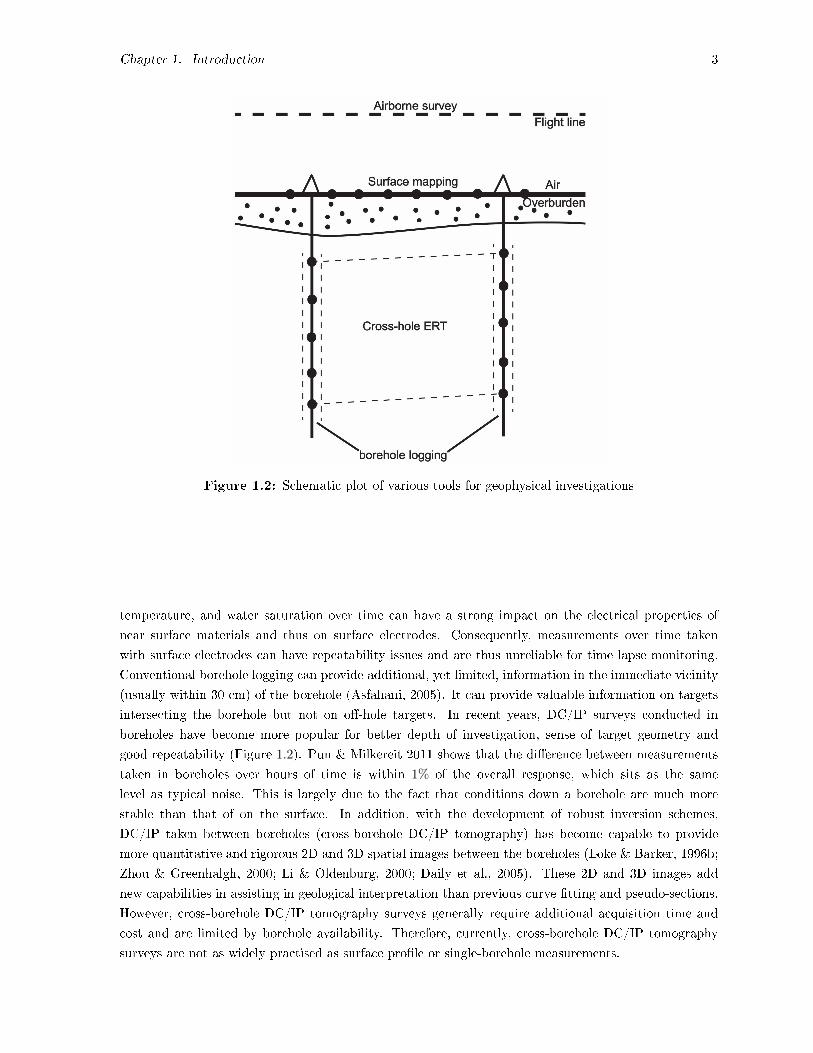
1.2 Schematic plot of various tools for geophysical investigations . . . . . . . . . . . . . . . . . 3
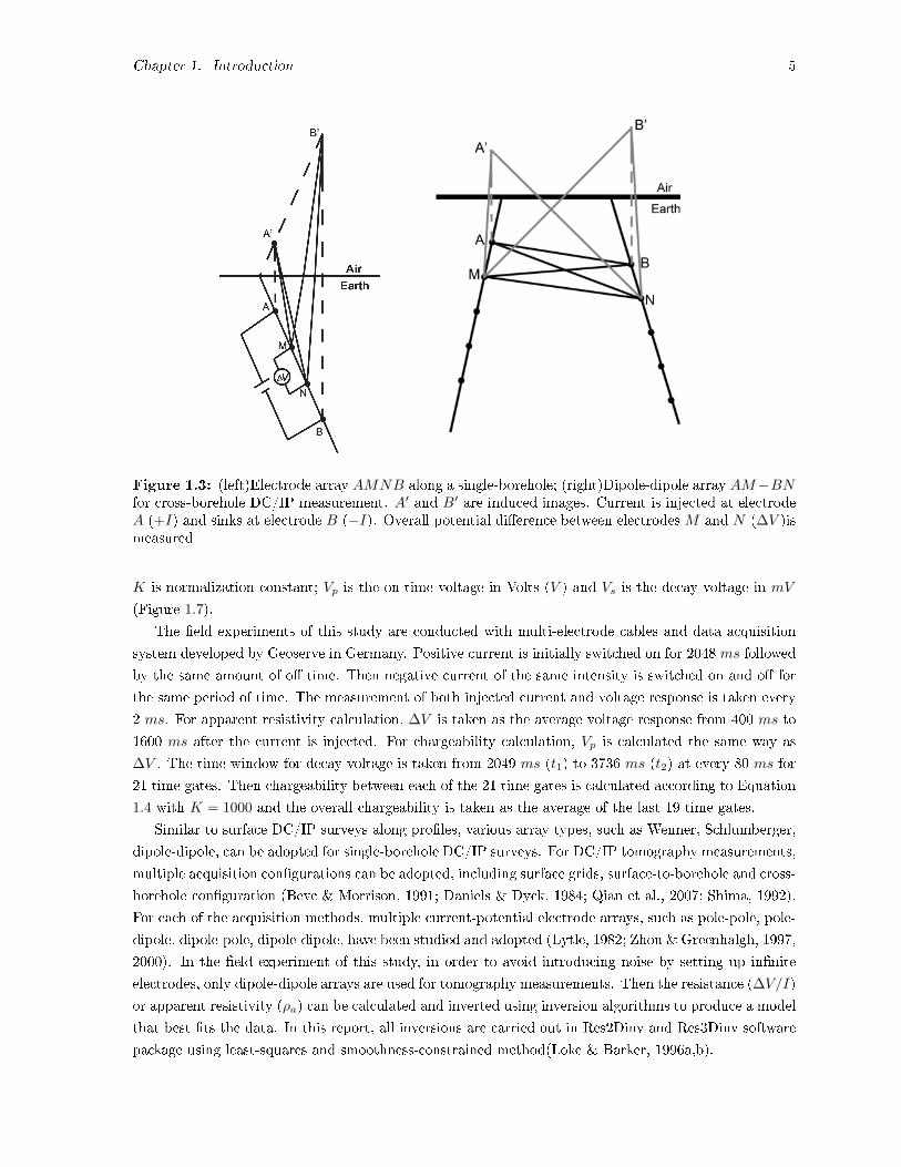
1.3 (left)Electrode array AMNB along a single-borehole; (right)Dipole-dipole array AM −BN for cross-borehole DC/IP measurement. A′ and B′ are induced images. Current is
injected at electrode A (+I) and sinks at electrode B (−I). Overall potential dierencebetween electrodes M and N (∆V )is measured . . . . . . . . . . . . . . . . . . . . . . . . 5
1.4 Schematic plot of electrode layouts for surface, borehole and surface-to-borehole DC/IP
surveys. Black circles represent positions of electrodes . . . . . . . . . . . . . . . . . . . . 6
1.5 Time-domain waveform of DC/IP data example with minimal IP eect; (top) injected
current; (bottom) voltage response . . . . . . . . . . . . . . . . . . . . . . . . . . . . . . . 6
1.6 Time-domain waveform of DC/IP data example with IP and potentially other distortion
eects; (top) injected current; (bottom) voltage response . . . . . . . . . . . . . . . . . . . 7
1.7 Schematic plot of voltage response illustrating chargeability calculation (modied from
Zonge et al. 2005) . . . . . . . . . . . . . . . . . . . . . . . . . . . . . . . . . . . . . . . . 7
2.1 Schematic plot of near surface boreholes at dierent dip angles. Solid black circles denote
positions of electrodes . . . . . . . . . . . . . . . . . . . . . . . . . . . . . . . . . . . . . . 9
2.2 Schematic plots of (left) idealized cross-borehole DC/IP tomography survey geometry and
(right) actual survey geometry using existing exploration boreholes . . . . . . . . . . . . . 9
2.3 Normalized geometry factor nkf as a function of depth of Wenner array. Numbers in the
legend are dip angles of the boreholes (in degrees). 0.5 corresponds to half-space scenario
and 1.0 corresponds to full-space scenario. z is depth . . . . . . . . . . . . . . . . . . . . 10
2.4 Normalized geometry factor nkv as a function of depth of Wenner array. Numbers in the
legend are dip angles of the boreholes (in degrees). 1.0 corresponds to a vertical borehole
scenario . . . . . . . . . . . . . . . . . . . . . . . . . . . . . . . . . . . . . . . . . . . . . . 10
2.5 Normalized geometry factor nkf as a function of depth for cross-borehole array AM−BN .
Numbers in the legend are dip angles of the boreholes (in degrees). 0.5 corresponds to half-
space scenario and 1.0 corresponds to full-space scenario. z is depth. Electrode spacing a
is 16m. Two boreholes are separated by 32m on the surface . . . . . . . . . . . . . . . . . 11
vi

2.6 Normalized geometry factor nfv as a function of depth of for cross-borehole array AM −BN . Numbers in the legend are dip angles of the boreholes (in degrees). 1.0 corresponds
to a vertical borehole scenario. z is depth. Electrode spacing a is 16m. Two boreholes
are separated by 32m on the surface . . . . . . . . . . . . . . . . . . . . . . . . . . . . . . 11
2.7 Schematic plot of cross-borehole acquisition geometry. . . . . . . . . . . . . . . . . . . . . 12
2.8 Normalized geometry factor nkf as a function of depth of for cross-borehole array AM −BN . Numbers in the legend are dip angles of the boreholes (in degrees). 1.0 corresponds
to a vertical borehole scenario. z is depth. Two boreholes are separated by 8m on the
surface . . . . . . . . . . . . . . . . . . . . . . . . . . . . . . . . . . . . . . . . . . . . . . 12
2.9 Normalized geometry factor nkv as a function of depth of for cross-borehole array AM −BN . Numbers in the legend are dip angles of the boreholes (in degrees). 1.0 corresponds
to a vertical borehole scenario. z is depth. Two boreholes are separated by 8m on the
surface . . . . . . . . . . . . . . . . . . . . . . . . . . . . . . . . . . . . . . . . . . . . . . 12
2.10 Schematic plot of cross-borehole acquisition geometry. . . . . . . . . . . . . . . . . . . . . 13
2.11 The two-layer model. C denotes current electode; P denotes voltage electrode. The
thickness of the water is d. All electrodes are on the water-Earth interface. . . . . . . . . 14
2.12 Apparent resistivity pseudo-sections at the bottom of the Ogilvie's lake at Deep River in
the summer. (a) calculated without correction for deviation eect and water layer; (b)
calculated with corrected geometry factor; (c) dierence between (a) and (b). (a), (b) are
in logarithmic scale while (c) is in natural number scale. . . . . . . . . . . . . . . . . . . . 16
3.1 2D color scheme combining resistivity and chargeability data . . . . . . . . . . . . . . . . 19
3.2 (Apparent resistivity (left) and chargeability (right) pseudo-section along borehole W121
(Schlumberger array). Resistivity is in log10(Ωm). Chargeability is in mV/V . Electrode
spacing is 4m . . . . . . . . . . . . . . . . . . . . . . . . . . . . . . . . . . . . . . . . . . . 20
3.3 Apparent resistivity (left) and chargeability (right) pseudo-sections along borehole W128
(Schlumberger array). Resistivity is in log10(Ωm). Chargeability is in mV/V . Electrode
spacing is 8m . . . . . . . . . . . . . . . . . . . . . . . . . . . . . . . . . . . . . . . . . . . 20
3.4 Apparent resistivity (left) and chargeability (right) pseudo-sections along borehole W130
(Schlumberger array). Resistivity is in log10(Ωm). Chargeability is in mV/V . Electrode
spacing is 8m . . . . . . . . . . . . . . . . . . . . . . . . . . . . . . . . . . . . . . . . . . . 21
3.5 (left) Resistivity tomography inversion result; (right) chargeability tomography inversion
result in commonly used RGB color scheme. Resistivity is in log10(Ωm) and chargeability
is in natural number scale (mV/V ). The horizontal axis is distance on the surface in
meters. Black solid lines represent positions of boreholes where the measurements were
taken. Borehole numbers from left to right are W130, W121 and W128 . . . . . . . . . . 21
3.6 Resistivity tomography in blue to green color scheme and chargeability tomography in
black to red color scheme . . . . . . . . . . . . . . . . . . . . . . . . . . . . . . . . . . . . 21
3.7 Combined resistivity and chargeability result in the new 2D color scheme. Resistivity is
in log10(Ωm) and chargeability is in mV/V . . . . . . . . . . . . . . . . . . . . . . . . . . 22
3.8 Apparent resistivity (left) and chargeability (right) pseudo-sections along borehole NRS130075
(Schlumberger array). Resistivity is in log10(Ωm). Chargeability is in mV/V . Electrode
spacing is 4m . . . . . . . . . . . . . . . . . . . . . . . . . . . . . . . . . . . . . . . . . . . 22
vii

3.9 Apparent resistivity (left) and chargeability (right) pseudo-sections along borehole NRS170143
(Schlumberger array). Resistivity is in log10(Ωm). Chargeability is in mV/V . Electrode
spacing is 8m . . . . . . . . . . . . . . . . . . . . . . . . . . . . . . . . . . . . . . . . . . . 23
3.10 Apparent resistivity (left) and chargeability (right) pseudo-sections along borehole NRS170100
(Schlumberger array). Resistivity is in log10(Ωm). Chargeability is in mV/V . Electrode
spacing is 16m . . . . . . . . . . . . . . . . . . . . . . . . . . . . . . . . . . . . . . . . . . 23
3.11 Apparent resistivity (left) and chargeability (right) pseudo-sections along borehole NRS170162
(Schlumberger array). Resistivity is in log10(Ωm). Chargeability is in mV/V . Electrode
spacing is 16m . . . . . . . . . . . . . . . . . . . . . . . . . . . . . . . . . . . . . . . . . . 24
3.12 (left) Resistivity tomography inversion result; (right) chargeability inversion result in com-
monly used RGB color scheme. Resistivity is in log10(Ωm) and chargeability is in mV/V .
The horizontal axis is distance in the tunnel in meters. Black solid lines represent posi-
tions of boreholes where the measurements were taken. Borehole numbers from left to
right are NRS170143 and NRS170100 . . . . . . . . . . . . . . . . . . . . . . . . . . . . . 24
3.13 Resistivity tomography in blue to green color scheme and chargeability tomography in
black to red color scheme between NRS170143 and NRS170100 . . . . . . . . . . . . . . . 24
3.14 Combined resistivity and chargeability tomography result in the new 2D color scheme
between NRS170143 and NRS170100. Resistivity is in log10(Ωm) and chargeability is in
mV/V . . . . . . . . . . . . . . . . . . . . . . . . . . . . . . . . . . . . . . . . . . . . . . 25
3.15 Schematic plot of a sphere anomaly of radius rsph, resistivity ρ1 located between two
boreholes in a homogeneous half-space of resistivity ρ2 (adopted from Lytle., 1982). The
center of the sphere is the origin of the spherical coordinate system . . . . . . . . . . . . . 26
3.16 Apparent resistivity of the sphere model with dipole-dipole array AM − BN (left) and
AM −NB (right) . . . . . . . . . . . . . . . . . . . . . . . . . . . . . . . . . . . . . . . . 27
3.17 Apparent resistivity perturbation due a conductive sphere between borehole with dipole-
dipole array AM −BN and AM −NB. AM is xed at 50m at borehole 1 while BN or
NB is shifted along the other borehole . . . . . . . . . . . . . . . . . . . . . . . . . . . . 28
3.18 Apparent resistivity perturbation due a conductive sphere between borehole with pole-
dipole array AM − B and AM −N . AM is xed at 50m at borehole 1 while B or N is
shifted along the other borehole . . . . . . . . . . . . . . . . . . . . . . . . . . . . . . . . 28
3.19 Comparison of apparent resistivity along the borehole acquired with dipole-pole AM −Nand dipole-dipole AM −BN array . . . . . . . . . . . . . . . . . . . . . . . . . . . . . . . 29
3.20 Percentage of variation in apparent resistivity due a spherical anomaly between boreholes
at various borehole separations and resistivity contrasts . . . . . . . . . . . . . . . . . . . 29
4.1 3D DC/IP survey acquisition geometry at an exploration site of Canadian Malartic Mine.
BR stands for borehole and L stands for line . . . . . . . . . . . . . . . . . . . . . . . . . 32
4.2 Apparent resistivity (left) and chargeability (right) pseudo-section of L1 (Schlumberger
array). Resistivity is in log10(Ωm). Chargeability is in mV/V . Electrode spacing is 4m . 33
4.3 Apparent resistivity (left) and chargeability (right) pseudo-section of L2 (Schlumberger
array). Resistivity is in log10(Ωm). Chargeability is in mV/V . Electrode spacing is 4m . 33
4.4 Apparent resistivity (left) and chargeability (right) pseudo-section of L3 (Schlumberger
array). Resistivity is in log10(Ωm). Chargeability is in mV/V . Electrode spacing is 4m . 33
viii
4.5 Waveform examples from L3 of injection current and voltage response without (left) and
with (right) IP and other distortion eects from L3 . . . . . . . . . . . . . . . . . . . . . 34
4.6 Waveforms of injection current and reversed voltage response with IP eect from voltage
reversal zone at 50m of L3 . . . . . . . . . . . . . . . . . . . . . . . . . . . . . . . . . . . 34
4.7 Waveforms of injection current and voltage response with IP eect of reversed polarity . 35
4.8 Apparent resistivity (left) and chargeability (right) pseudo-section along BR1 (Schlum-
berger array). Resistivity is in log10(Ωm). Chargeability is in mV/V . Electrode spacing
is 8m . . . . . . . . . . . . . . . . . . . . . . . . . . . . . . . . . . . . . . . . . . . . . . . 35
4.9 Apparent resistivity (left) and chargeability (right) pseudo-section along BR2 (Schlum-
berger array). Resistivity is in log10(Ωm). Chargeability is in mV/V . Electrode spacing
is 8m . . . . . . . . . . . . . . . . . . . . . . . . . . . . . . . . . . . . . . . . . . . . . . . 36
4.10 Apparent resistivity (left) and chargeability (right) pseudo-section along BR3 (Schlum-
berger array). Resistivity is in log10(Ωm). Chargeability is in mV/V . Electrode spacing
is 16m . . . . . . . . . . . . . . . . . . . . . . . . . . . . . . . . . . . . . . . . . . . . . . . 36
4.11 Resistivity tomography between BR1(Left) and BR2(right) in log10(Ωm). Electrode spac-
ing is 8m . . . . . . . . . . . . . . . . . . . . . . . . . . . . . . . . . . . . . . . . . . . . . 37
4.12 Chargeability tomography between BR1(Left) and BR2(right) in mV/V . Electrode spac-
ing is 8m . . . . . . . . . . . . . . . . . . . . . . . . . . . . . . . . . . . . . . . . . . . . . 37
4.13 Resistivity tomography between BR1(Left) and BR2(right) in log10(Ωm). Data is acquired
with dipole-dipole array AM −NB. Electrode spacing is 8m . . . . . . . . . . . . . . . . 37
4.14 Chargeability tomography between BR1(Left) and BR2(right) inmV/V . Data is acquired
with dipole-dipole array AM −NB. Electrode spacing is 8m . . . . . . . . . . . . . . . . 37
4.15 Resistivity tomography between BR1(Left) and BR3(right most) in log10(Ωm). BR2 is
also plotted for reference. Electrode spacing is 16m. BR3 is the edge of the image at 200m 38
4.16 Chargeability tomography between BR1(Left) and BR3(right most) in mV/V . BR2 is
also plotted for reference. Electrode spacing is 16m. BR3 is the edge of the image at 200m 38
4.17 Resistivity tomography between L1(Left) and L2(right) in log10(Ωm). Electrode spacing
is 4m . . . . . . . . . . . . . . . . . . . . . . . . . . . . . . . . . . . . . . . . . . . . . . . 39
4.18 Chargeability tomography between L1(Left) and L2(right) in mV/V . Electrode spacing
is 4m . . . . . . . . . . . . . . . . . . . . . . . . . . . . . . . . . . . . . . . . . . . . . . . 39
4.19 Resistivity tomography between L1(Left) and L3 (right most) in log10(Ωm). Electrode
spacing is 4m . . . . . . . . . . . . . . . . . . . . . . . . . . . . . . . . . . . . . . . . . . . 39
4.20 Chargeability tomography between L1(Left) and L3 (right most) in mV/V . Electrode
spacing is 4m . . . . . . . . . . . . . . . . . . . . . . . . . . . . . . . . . . . . . . . . . . . 39
4.21 3D fence diagram of resistivity (left) and chargeability (right) distribution around L1, L2
and BR1, BR2 . . . . . . . . . . . . . . . . . . . . . . . . . . . . . . . . . . . . . . . . . . 40
4.22 3D view of various anomaly distrition with respect to the acquistion conguration . . . . 41
A.1 Percentage of change in electrical resistivity from 0 to 30 C based on Equation A.1 and
A.2 . . . . . . . . . . . . . . . . . . . . . . . . . . . . . . . . . . . . . . . . . . . . . . . . 48
A.2 Inverted resistivity pseudo-section of line 4 on Ogilvie's lake in the summer (top) and in
the winter(bottom). The array type is Schlumberger and electrode spacing is 4m . . . . . 48
A.3 Modied inverted resistivity pseudo-section of line 4 on Ogivile's lake in the winter based
on Equation A.1 (top) and A.2 (bottom) . . . . . . . . . . . . . . . . . . . . . . . . . . . 49
ix

B.1 Apparent resistivity along L1 and BR1 in log10(Ωm) . . . . . . . . . . . . . . . . . . . . . 51
B.2 Chargeability along L1 and BR1 in mV/V . . . . . . . . . . . . . . . . . . . . . . . . . . 51
B.3 Apparent resistivity along L2 and BR2 in log10(Ωm) . . . . . . . . . . . . . . . . . . . . . 51
B.4 Chargeability along L2 and BR2 in mV/V . . . . . . . . . . . . . . . . . . . . . . . . . . 51
B.5 Apparent resistivity along L1 and BR2 in log10(Ωm) . . . . . . . . . . . . . . . . . . . . . 51
B.6 Chargeability along L1 and BR2 in mV/V . . . . . . . . . . . . . . . . . . . . . . . . . . 51
B.7 Apparent resistivity along L2 and BR1 in log10(Ωm) . . . . . . . . . . . . . . . . . . . . . 52
B.8 Chargeability along L2 and BR1 in mV/V . . . . . . . . . . . . . . . . . . . . . . . . . . 52
B.9 Apparent resistivity along L3 and BR3 log10(Ωm) . . . . . . . . . . . . . . . . . . . . . . 52
B.10 Chargeability along L3 and BR3 in mV/V . . . . . . . . . . . . . . . . . . . . . . . . . . 52
B.11 Apparent resistivity along L1 and BR3 log10(Ωm) . . . . . . . . . . . . . . . . . . . . . . 52
B.12 Chargeability along L1 and BR3 in mV/V . . . . . . . . . . . . . . . . . . . . . . . . . . 52
C.1 Schematic plots of equipotentials (dashed lines) of array AMNB. a(top) in a homogeneous
full-space; b(bottom) disturbed by resistivity anomaly and give reversed voltage response 54
C.2 Schematic plots of a capacitor with reversed current ow in a 3D Earth . . . . . . . . . . 55
C.3 Simplied circuit digram representing the layered Earth materials as a capacitor in parallel
with resistors . . . . . . . . . . . . . . . . . . . . . . . . . . . . . . . . . . . . . . . . . . . 55
C.4 Apparent resistivity in log10(Ωm)(left), chargeability in mV/V (right) pseudo-sections of
NRS170143 . . . . . . . . . . . . . . . . . . . . . . . . . . . . . . . . . . . . . . . . . . . . 55
C.5 Cross-correlation coecient pseudo-section of NRS170143 . . . . . . . . . . . . . . . . . . 56
C.6 Apparent resistivity in log10(Ωm) (left), chargeability in mV/V (right) pseudo-sections
of NRS170100 . . . . . . . . . . . . . . . . . . . . . . . . . . . . . . . . . . . . . . . . . . 56
C.7 Cross-correlation coecient pseudo-section of NRS170100 . . . . . . . . . . . . . . . . . . 57
C.8 Apparent resistivity in log10(Ωm) (left), chargeability in mV/V (right) pseudo-sections
of L3 . . . . . . . . . . . . . . . . . . . . . . . . . . . . . . . . . . . . . . . . . . . . . . . 57
C.9 Cross-correlation coecient pseudo-section of L3 . . . . . . . . . . . . . . . . . . . . . . . 58
x

List of Tables
1 List of Symbols . . . . . . . . . . . . . . . . . . . . . . . . . . . . . . . . . . . . . . . . . . xi
Table 1: List of Symbols
t timeσ conductivityρ resistivityµ magnetic permeabilitya electrode spacingI currentm chargeability
U , V potentialθ latitudinal angle in spherical coordinateφ longitudinal angle in spherical coordinateΦ cross-correlation coecientτ time lagR distance between current and potential electrodek geometric factorrsph radius of spherers distance between the center of the sphere center and current electroder distance between the potential electrode and center of the sphereR distance between the current and potential electrode
A, B current electrodeM , N potential electrodeAMNB Wenner, Schlumberger array
AM −BN , AM −NB cross-borehole dipole-dipole arrayAM −N , AM −B cross-borehole dipole-pole array
Pmn associate Legendre function of the rst kindλ dummy variable of integrationJ0 zeroth order Bessel function of the rst kind
αi, βi transmission, reection coecientε temperature compensation factor
xi

Chapter 1
Introduction
1.1 Background
For near surface earth materials within lithostatic pressure, the bulk electrical resistivity is not only
controlled by conductive materials, but also largely inuenced by porosity, permittivity, fracturing and
uid content (Ward, 1990). In general, presence of porosity, permittivity and fracturing will increase
the bulk electrical resistivity. However, uid induced into these open spaces may further complicate the
situation by further increasing (e.g. oil) or decreasing (e.g. water) the resistivity of the material. Brace
et al. 1965 report that the electrical resistivity of water-saturated crystalline rocks generally increases
with increasing hydrostatic pressure. From 0 kb to 10 kb, the increase can be as much as three orders
of magnitude. For partially saturated rocks, on the other hand, the resistivity decreases with increasing
pressure. The resistivity-pressure variation becomes more complicated with the presence of conductive
materials. Increase in pressure initially decreases resistivity and then has almost no eect (Brace &
Orange, 1968b). Further experiments show that, for water saturated crystalline rock under compressive
stress, resistivity rst slightly increases until half the fracture stress and then decreases. However, for
sandstone under stress, either fully or partially saturated, the resistivity decreases with increasing stress
until fracturing occurs (Kate, 1994). Nevertheless, changes in bulk electrical resistivity of earth materials
can be used as an indicator of changes in stress and structures.
By Archie′s law, porosity and induced uid have a direct impact on the bulk resistivity (Archie,
1942). Glover et al. 2000; Glover 2010 proposes a modied Archies law by taking both the pore uid
and the hosting rock as conductive phases,
ρa = ρwφ−m + ρs(1− φ)−p (1.1)
where p = log(1−φm)log(1−φ) ; ρs is the resistivity of the host rock; porosity φ is fully saturated with uid of
resistivity ρw; m is cementation exponent; ρa is the resulting bulk resistivity. Figure 1.1 depicts the
calculated bulk resistivity of a rock at dierent porosities as a function of conductivity of the induced
pore uid.
Figure 1.1 shows that even for uid of low conductivity (10−2 S/m - 10−1 S/m), saturating porosity
of small volume fractions (0.5% - 1.0%), can change bulk resistivity can by up to 10 %. This amount of
change sits well above typical instrumental noise level (1 %) and can be well captured by direct current
(DC) resistivity imaging. It is also noted that, with pore uid of higher conductivity (greater than 10
1

Chapter 1. Introduction 2
Figure 1.1: The bulk resistivity of a rock as a function of conductivity of induced pore uid at dierentporosities (m = 2). The numbers in the legend are volume fractions of porosity. The lower end of theconductivity of uid 10−2 S/m corresponds to fresh water and the higher end 102 S/m corresponds tobrine water. Percentage is ρa/ρs × 100%
S/m) and porosity higher than 5%, the bulk resistivity is primarily controlled by the conductivity of the
uid. Under this circumstance, the pore uid acts as the main conducting phase and the bulk resistivity
variation under stress or pressure should be primarily attributed to changes in pore space.
Therefore, in addition to mineral and ground water exploration, DC resistivity method has been
demonstrated to be capable to track time lapse changes for geotechnical and environmental monitoring,
such as waste leakage, air sparging, steam injection and tracer experiment (Daniels & Dyck, 1984;
LaBrecque et al., 1996; Muller et al., 2010; Nimmer et al., 2007; Ramirez et al., 1993; Schima et al.,
1996).
The induced polarization (IP) eect was rst reported by Conrad Schlumberger in the early 1900s and
is usually measured together with DC resistivity measurement (Schlumberger, 1920). When the current
injection is being switched on and o, in time domain, it is a phenomenon observed as a voltage delay
while in frequency domain as a phase shift (Summer, 1976; Ward, 1990). Although without knowing the
nature of the IP eect, it has been demonstrated to be useful in ground water exploration and detecting
non-conductive targets, such as disseminated sulphide related gold and copper mineralization (Binley &
Kemna, 2005; Seigel, 1971; Hallof et al., 1990; Seigel et al., 2007). The IP eect can be aected by a
range of parameters, such as lithology, open spaces and pore uid chemistry (Binley & Kemna, 2005;
Ward, 1990). In addition to mineral exploration, some eort has also been put into investigating its
capability in dealing with time lapse monitoring problems (Gallas et al., 2011; Ghorban et al., 2008;
Slater & Sandberg, 2000).
Over the last century, surface DC/IP surveys have been well utilized for near surface imaging. Despite
their popularity, such surveys are limited by the depth of penetration, especially with the presence of
conductive overburden, and repeatability problems (Oldenburg & Li, 1999; Pun & Milkereit, 2011). It
has been suggested that, for a target in a homogeneous half-space, one cannot expect to delineate target
whose depth is greater than its dimension (Van, 1953; Asfahani, 2005). Also, variation of weather,
Chapter 1. Introduction 3
Figure 1.2: Schematic plot of various tools for geophysical investigations
temperature, and water saturation over time can have a strong impact on the electrical properties of
near surface materials and thus on surface electrodes. Consequently, measurements over time taken
with surface electrodes can have repeatability issues and are thus unreliable for time lapse monitoring.
Conventional borehole logging can provide additional, yet limited, information in the immediate vicinity
(usually within 30 cm) of the borehole (Asfahani, 2005). It can provide valuable information on targets
intersecting the borehole but not on o-hole targets. In recent years, DC/IP surveys conducted in
boreholes have become more popular for better depth of investigation, sense of target geometry and
good repeatability (Figure 1.2). Pun & Milkereit 2011 shows that the dierence between measurements
taken in boreholes over hours of time is within 1% of the overall response, which sits as the same
level as typical noise. This is largely due to the fact that conditions down a borehole are much more
stable than that of on the surface. In addition, with the development of robust inversion schemes,
DC/IP taken between boreholes (cross-borehole DC/IP tomography) has become capable to provide
more quantitative and rigorous 2D and 3D spatial images between the boreholes (Loke & Barker, 1996b;
Zhou & Greenhalgh, 2000; Li & Oldenburg, 2000; Daily et al., 2005). These 2D and 3D images add
new capabilities in assisting in geological interpretation than previous curve tting and pseudo-sections.
However, cross-borehole DC/IP tomography surveys generally require additional acquisition time and
cost and are limited by borehole availability. Therefore, currently, cross-borehole DC/IP tomography
surveys are not as widely practised as surface prole or single-borehole measurements.

Chapter 1. Introduction 4
1.2 Method
In measuring the bulk resistivity of earth materials, a pair of current electrodes are used to inject current
(I) into surrounding materials. The resulting potential dierence (∆V ) is measured at a another pair of
potential electrodes (Figure 1.3). The current-potential electrode pairs compose an electrode array. For
borehole DC/IP surveys, the electrode arrays at dierent spacings are moved along the borehole(s) for
single-borehole and cross-borehole DC/IP measurements.
In this study, the following symbol convention is adopted. The italic letter A denotes the current
source (+I) and B denotes the current sink (−I). M and N denote potential electrodes. For cross-
borehole DC/IP tomography, electrodes in dierent boreholes are separated by dash line −. For exampleelectrode array AM − BN represent an array in which electrodes A and M are in the left hand side
borehole and A is on top of M ; B and N are in the right hand side borehole and B is on top of N
(Figure 1.3).
For an electrode planted on the surface of a homogeneous half-space, all injected currents are restricted
to ow into the Earth side as the air is non-conductive. For an electrode in a homogeneous full-space, on
the other hand, injected currents are free to ow in all directions (Figure 1.4). As a result, the geometry
factor, which accounts for the electrode array conguration, for the full-space case is essentially twice
the half space case. For resistivity measurements taken in near surface boreholes, we are essentially
dealing with a situation between half-space and full-space. For an electrode array AMNB along a near
surface borehole (Figure 1.3), electrical images A' and B' are induced with equal current intensity at
equal distances to the air-Earth interface above the Earth (Van & Cook, 1966; Telford & Sheri, 1990).
Both electrical images will also results in potentials at M and N . Then the expression for potential
dierence between M and N is
∆V =ρaI
4π(
1
AM+
1
A′M− 1
BM− 1
B′M− 1
AN− 1
A′N+
1
BN+
1
B′N) (1.2)
The apparent resistivity ρa can then be calculated by rearranging Equation 1.2
ρa =∆V
Ik, k = 4π/(
1
AM+
1
A′M− 1
BM− 1
B′M− 1
AN− 1
A′N+
1
BN+
1
B′N) (1.3)
where k is the geometry factor for a certain electrode array. The apparent resistivity will approach the
true resistivity of the half- or full-space if the dimension of the target is much smaller than the electrode
spacing and/or the distance from the target to the electrode array.
Figure 1.5 and 1.6 show time-domain DC/IP data examples with minimal and signicant IP eect.
When the current is on, a constant voltage response is produced and when the current is switched o,
the voltage response instantly goes back to zero. However, some earth materials act as capacitors and
the voltage response respond to current variation with a time delay. As shown in Figure 1.6, the voltage
gradually increases to its maximum before the injected current is switched o. After the current is
switched o, the voltage gradually decays back to zero. The time-domain IP eect can be quantied as
chargeability m (Zonge et al., 2005)
m =K
Vp
∫ t2
t1
Vsdt (1.4)
where m is chargeability in mV/V ; t1 and t2 are time gates between which the voltage is measured;
Chapter 1. Introduction 5
Figure 1.3: (left)Electrode array AMNB along a single-borehole; (right)Dipole-dipole array AM−BNfor cross-borehole DC/IP measurement. A′ and B′ are induced images. Current is injected at electrodeA (+I) and sinks at electrode B (−I). Overall potential dierence between electrodes M and N (∆V )ismeasured
K is normalization constant; Vp is the on-time voltage in Volts (V ) and Vs is the decay voltage in mV
(Figure 1.7).
The eld experiments of this study are conducted with multi-electrode cables and data acquisition
system developed by Geoserve in Germany. Positive current is initially switched on for 2048 ms followed
by the same amount of o time. Then negative current of the same intensity is switched on and o for
the same period of time. The measurement of both injected current and voltage response is taken every
2 ms. For apparent resistivity calculation, ∆V is taken as the average voltage response from 400 ms to
1600 ms after the current is injected. For chargeability calculation, Vp is calculated the same way as
∆V . The time window for decay voltage is taken from 2049 ms (t1) to 3736 ms (t2) at every 80 ms for
21 time gates. Then chargeability between each of the 21 time gates is calculated according to Equation
1.4 with K = 1000 and the overall chargeability is taken as the average of the last 19 time gates.
Similar to surface DC/IP surveys along proles, various array types, such as Wenner, Schlumberger,
dipole-dipole, can be adopted for single-borehole DC/IP surveys. For DC/IP tomography measurements,
multiple acquisition congurations can be adopted, including surface grids, surface-to-borehole and cross-
borehole conguration (Bevc & Morrison, 1991; Daniels & Dyck, 1984; Qian et al., 2007; Shima, 1992).
For each of the acquisition methods, multiple current-potential electrode arrays, such as pole-pole, pole-
dipole, dipole-pole, dipole-dipole, have been studied and adopted (Lytle, 1982; Zhou & Greenhalgh, 1997,
2000). In the eld experiment of this study, in order to avoid introducing noise by setting up innite
electrodes, only dipole-dipole arrays are used for tomography measurements. Then the resistance (∆V/I)
or apparent resistivity (ρa) can be calculated and inverted using inversion algorithms to produce a model
that best ts the data. In this report, all inversions are carried out in Res2Dinv and Res3Dinv software
package using least-squares and smoothness-constrained method(Loke & Barker, 1996a,b).

Chapter 1. Introduction 6
Figure 1.4: Schematic plot of electrode layouts for surface, borehole and surface-to-borehole DC/IPsurveys. Black circles represent positions of electrodes
Figure 1.5: Time-domain waveform of DC/IP data example with minimal IP eect; (top) injectedcurrent; (bottom) voltage response

Chapter 1. Introduction 7
Figure 1.6: Time-domain waveform of DC/IP data example with IP and potentially other distortioneects; (top) injected current; (bottom) voltage response
Figure 1.7: Schematic plot of voltage response illustrating chargeability calculation (modied fromZonge et al. 2005)

Chapter 2
Geometrical eect
Although the capability of DC/IP method in dealing with exploration and monitoring problems has been
demonstrated, previous studies generally assume the boreholes are drilled near vertically and dierent
boreholes are in the same plane as what is to be imaged. It is also assumed that, regardless of depth
from the surface, electrodes in a borehole are in a full-space scenario. However, for practical purposes,
boreholes are usually drilled at various dip angles and azimuths in order to maximize geological informa-
tion to be obtained (Figure 2.1, 2.2). For near-surface borehole DC/IP surveys in particular, we are also
dealing with a transition from half-space to full-space. Data processing and inversion without taking
such deviation eect can raise errors that are well above typical data noise levels (Oldenborger et al.,
2005; Yi et al., 2009). Such errors can be problematic in resolving high resolution structures, especially
for time-varying monitoring purposes. This chapter compares the geometry factors of dipping boreholes
with geometry factors calculated with full-space or vertical borehole assumptions for the single-borehole
and cross-borehole cases. Then a modied geometry factor is proposed to account for both the deviation
eect and the water layer for a underwater DC/IP survey.
2.1 Single-borehole
In order to examine the deviation eect, the geometry factor k along a deviated borehole is normalized
by the geometry factor in a full-space scenario (kf )
nkf = k/kf (2.1)
or in a vertical borehole scenario
nkv = k/kv (2.2)
Figure 2.3 and 2.4 depict the variation of normalized geometry factors of Wenner array as a function
of depth along boreholes dipping at various angles. Both gures show that the normalized geometry
factors converge to 1.0. Also, normalized geometry factors along shallow dipping boreholes show more
variation than near vertical ones. According to Figure 2.3, the transition from half-space to full-space
mostly occurs in the top 20 % of the boreholes, within which boreholes of all dip angles show signicant
variation. Even for a near vertical borehole dipping at 80 degrees, the total variation can be more than
15 %. In Figure 2.4, it is noted that the transition from deviated to vertical boreholes also mostly occurs
8

Chapter 2. Geometrical eect 9
Figure 2.1: Schematic plot of near surface boreholes at dierent dip angles. Solid black circles denotepositions of electrodes
Figure 2.2: Schematic plots of (left) idealized cross-borehole DC/IP tomography survey geometry and(right) actual survey geometry using existing exploration boreholes
within the rst 20 % of the boreholes. However, for boreholes with the same dip angles, the deviation
and half-space-full-space transition are only signicant for shallow dipping boreholes. For a borehole
dipping at 60 degrees, the total variation is less than 3 %. For a borehole with a steep dip angle of
80 degrees, the variation is basically within the typical instrumental noise level (1 %). It is also found
that, when the rst electrode is at depth of 100m, regardless of dip angle, the total variation in both
nkf and nkv becomes less than typical noise level and thus can be neglected. Similar variation pattern
is obtained with Schlumberger array.
2.2 Cross-borehole
The normalized geometry factors for cross-borehole array AM −BN are calculated in the same way as
the single-borehole case. Electrodes A and M are xed on the top of the left borehole while B and N
are moved from the top to the bottom in the other borehole. The depth of each plot point is calculated

Chapter 2. Geometrical eect 10
Figure 2.3: Normalized geometry factornkf as a function of depth of Wenner ar-ray. Numbers in the legend are dip angles ofthe boreholes (in degrees). 0.5 correspondsto half-space scenario and 1.0 corresponds tofull-space scenario. z is depth
Figure 2.4: Normalized geometry factor nkvas a function of depth of Wenner array. Num-bers in the legend are dip angles of the bore-holes (in degrees). 1.0 corresponds to a verticalborehole scenario
by averaging the depth of the four electrodes. The two boreholes dip at the same angle with opposite
azimuths. The results are shown in Figure 2.5 and 2.6.
Similarly as the single-borehole case (Figure 2.3), nkf shows a transition from half-space to full-space
scenario and most variation occurs within the top 20 % of the borehole (Figure 2.5 and 2.6). However,
nkf converges to 0.8 instead of 1.0. This suggests that the transition remains signicant throughout the
borehole and the full-space assumption over simplies the situation. nkv in Figure 2.6 also shows similar
behaviour as the single-borehole case with greater overall variation. Even for a steep dipping borehole
at 80 degrees, the overall variation, instead of being below noise level, is about 10 % and should be taken
into account. When the boreholes separation is smaller than spacing between current and potential
electrode in each borehole, a near singular behaviour occurs.
For electrode array AM −BN as depicted in Figure 2.7, the denominator of geometry factor g from
Equation 1.3 can be rearranged into
g = 2(1
a− 1
a
1√1 + (d/a)2
+1
a+ 2z− 1
a+ 2z
1√(1 + (d/a+ 2z)2
)
=2
a(1− 1√
1 + (d/a)2) +
2
a+ 2z(1− 1√
1 + (d/a+ 2z)2)
When borehole separation d is smaller than electrode separation a (d/a+ 2z < d/a < 1),
g ∼ 2
a(1− (1− 1
2(d/a)2)) +
2
a(1− (1− 1
2(d/a+ 2z))) =
d2
a3+
d2
(a+ 2z)2(2.3)
g becomes considerably small and k becomes a near singular point. Figure 2.9 depicts the variation of
nkv with depth when borehole separation d is one half of AM (AM = a). Because of near singular
behaviour of kv when AM and BN are at the same level, nnv behaves non-causally as observed as
signicant dips in 2.9. Similar behaviour is also seen in Figure 2.8 when the borehole is steeply dipping

Chapter 2. Geometrical eect 11
Figure 2.5: Normalized geometry factor nkfas a function of depth for cross-borehole arrayAM − BN . Numbers in the legend are dipangles of the boreholes (in degrees). 0.5 cor-responds to half-space scenario and 1.0 corre-sponds to full-space scenario. z is depth. Elec-trode spacing a is 16m. Two boreholes are sep-arated by 32m on the surface
Figure 2.6: Normalized geometry factor nfvas a function of depth of for cross-boreholearray AM − BN . Numbers in the legend aredip angles of the boreholes (in degrees). 1.0corresponds to a vertical borehole scenario. zis depth. Electrode spacing a is 16m. Twoboreholes are separated by 32m on the surface
at 80 degrees. Data acquired at such levels may not be eective signals from potential targets and results
in misinterpretation. Such behaviour disappears in boreholes dipping at smaller angles as separation
between boreholes becomes greater electrode spacing a. Therefore, it is recommended that extra care
should be taken when borehole separation is smaller than electrode spacing. Zhou & Greenhalgh 2000
reports that array AM −NB produces similar inversion results as AM − BN in their synthetic study.
As there is no singularity problem in geometry factor in array AM−NB, it can be used as an alternativeacquisition array when borehole separation is smaller than electrode spacing at certain levels.
On the other hand, for a cross-borehole acquisition geometry as in Figure 2.10, the potential due to
+I at A and −I at B at (x, z)
V (x, z) =ρI
4π(
1√z2 + x2
− 1√z2 + (d− x)2
) (2.4)
Then the horizontal eld at distance z below A in the left hand side borehole
E(z) = −∂V∂x|x=0=
ρI
4π
d
(z2 + d2)3/2(2.5)
Dierentiating equation 2.2 with respect to borehole separation d,
∂E(z)
∂d=ρI
4π
(z2 + d2)3/2 − 3(z2 + d2)1/2d2
(z2 + d2)3(2.6)
The optimal detecting depth with respect to borehole separation occurs when the above dierentiation

Chapter 2. Geometrical eect 12
Figure 2.7: Schematic plot of cross-borehole acquisition geometry.
Figure 2.8: Normalized geometry factor nkfas a function of depth of for cross-boreholearray AM − BN . Numbers in the legend aredip angles of the boreholes (in degrees). 1.0corresponds to a vertical borehole scenario. zis depth. Two boreholes are separated by 8mon the surface
Figure 2.9: Normalized geometry factor nkvas a function of depth of for cross-borehole ar-ray AM −BN . Numbers in the legend are dipangles of the boreholes (in degrees). 1.0 cor-responds to a vertical borehole scenario. z isdepth. Two boreholes are separated by 8m onthe surface

Chapter 2. Geometrical eect 13
Figure 2.10: Schematic plot of cross-borehole acquisition geometry.
goes to zero∂E(z)
∂d= 0⇒ z =
√2d (2.7)
and∂2E(
√2d)
∂2d< 0 (2.8)
Therefore, the maximum horizontal eld is reached at√
2 times the separation of the boreholes below the
current electrodes. However, the aforementioned singularity problem may arise with such conguration.
Therefore, for boreholes at small separation, the optimal electrode spacing should not be greater than
the borehole separation. After each set of measurements, the electrodes can be shifted by a portion of
AM to improve resolution and better delineate small scale features.
2.3 Application
A DC/IP monitoring project has been conducted at Ogilvie's lake, Deep River, Ontario. The lake is
believed to be closely related to a pristine shallow glaciouvial groundwater system (Shirokova & Ferris,
2013). Multiple proles of DC/IP surveys have been conducted both on top and at the bottom of the
lake. The lake bottom dips roughly at 10 degrees from the bank to the center of the lake, which is a
similar scenario as a shallow dipping borehole. In addition, for the latter case, the electrodes are laid at
the interface of lake water and sediments. The injected current, instead of all owing into homogeneous
Earth materials, splits into the water and the Earth. Therefore, the conventional apparent resistivity
formula (Equation 1.3) needs to be re-formulated to include the presence of a water layer. This scenario
is approximately equivalent to a two layered Earth problem where the electrodes locate at the interface
of the rst and second layer.
Van & Cook 1966 gives the potential due to a point source in a three layered Earth. Then Daniels
1978 extends the formulation to an n-layered case in a recursion relationship. Assuming the current
electrode to be a pole at the origin of cylindrical coordinates, for a point current source in layer 0 of

Chapter 2. Geometrical eect 14
Figure 2.11: The two-layer model. C denotes current electode; P denotes voltage electrode. Thethickness of the water is d. All electrodes are on the water-Earth interface.
resistivity ρ0 (Figure 2.11), the potential measured at P is,
Ui(r, zi) =Iρ04π
[
∫ +∞
0
(αieλzi + (βi + 1)e−λzi)J0(λr)dλ] (2.9)
Using the Lipschitz's integral, we get
Ui(r, zi) =Iρ04π
[1
r+
∫ +∞
0
(αieλzi + βie
−λzi)J0(λr)dλ] (2.10)
where I is injected current, r is the radial distance between a pair of current electrode and potential
electrode; αi, βi are transmittance and reection coecients in the ith layer; λ is the dummy variable
of integration; J0 is the zeroth order Bessel function of the rst kind. The rst part of Equation 2.10
is the primary part and is the same as the case where the electrode is in a homogeneous full-space.
The second part of the equation is the secondary part due to presence of non-resistive layer above the
current electrode. The α term is the part that decays upwards and the β term is the part that decays
downwards.
However, Daniels 1978's formulation is unnecessarily complicated by having current and potential
electrodes in arbitrary layers and is mainly used for modelling and interpretation. In this study, the
scenario can be simplied by replacing all layers above the current electrode by a water layer of thickness
d of resistivity rho−1 and all layers below the current electrode by a homogeneous half-space of resistivity
ρ0 (Figure 2.11). As the potential electrode is also located at the water-Earth interface, Equation 2.10
can be further simplied by letting zi = 0. Two typos are noted in Daniels's paper and are corrected in
the following formulation. The simplied model is depicted in Figure 2.11.
Consequently, Equation 2.10 is simplied to be
U−1(r, z−1) =Iρ04π
[1
r+
∫ +∞
0
(α−1eλz−1 + β−1e
−λz−1)J0(λr)dλ] (2.11)
in the water layer and
U0(r, z0) =Iρ04π
[1
r+
∫ +∞
0
(α0eλz0 + β0e
−λz0)J0(λr)dλ] (2.12)

Chapter 2. Geometrical eect 15
in the Earth layer. (α−1 β−1) and (α0 β0) are undetermined coecients to be solved by applying
appropriate boundary conditions.
First of all, the current across the air-water interface must be zero as the air is non-conductive. As
the current density is proportional to the vertical derivation of potential (Jz = − 1ρ∂U∂z ), then
∂U−1∂z|z−1=d =
Iρ04π
[
∫ +∞
0
(λα−1eλd − λ(β−1 + 1)e−λd)J0(λr)dλ] = 0 (2.13)
Setting the integrand to be zero.
α−1eλd − (β−1 + 1)e−λd = 0 =⇒ α−1 = (β−1 + 1)e−2λd (2.14)
Secondly, the potential at the water-Earth interface must be continuous U−1|z−1=0 = U0|z0=0 so that
α−1 + β−1 = α0 + β0 (2.15)
In addition, the secondary part of the vertical current density should be continuous across the water-
Earth interface1
ρ−1
∂U−1∂z|z−1=0 =
1
ρ0
∂U0
∂z|z0=0 (2.16)
Equating the integrands and gets
ρ0λ(α−1 − β−1) = ρ−1λ(α0 − β0) =⇒ ρ0ρ−1
(α−1 − β−1) = α0 − β0 (2.17)
Lastly, U0 should go to zero as z0 goes to innity and go to ρ0I4π near the source. Therefore in layer 0
α0 = 0 (2.18)
Solving Equation 2.3 to 2.18 for (α−1 β−1),(α0 β0) and get
α−1 =e−2λd(ρ−1 − ρ0)
e−2λd(ρ−1 + ρ0) + (ρ−1 − ρ0), β−1 = − e−2λd(ρ−1 + ρ0)
e−2λd(ρ−1 + ρ0) + (ρ−1 − ρ0)(2.19)
and
α0 = 0, β0 = − 2e−2λdρ0e−2λd(ρ−1 + ρ0) + (ρ−1 − ρ0)
(2.20)
Then
U0|z0=0 =Iρ04π
[1
r− 2
ρ0ρ−1 + ρ0
∫ +∞
0
e−2λd
e−2λd + ρ−1−ρ0ρ−1+ρ0
J0(λr)dλ] (2.21)
Unfortunately, there is not analytical solution to the integral, it has to be calculated numerically.
For a four electrode array AMNB, where current is injected at A and sinks at B, potential is
measured at M and N , r is replaced with AM , BM , AN and BN :
∆U =Iρa4π
(1
AM− 1
BM− 1
AN+
1
BN−
2ρ0
ρ−1 + ρ0
∫ +∞
0
e−2λd
e−2λd + ρ−1−ρ0ρ−1+ρ0
[J0(λAM)− J0(λBM)− J0(λAN) + J0(λBN)]dλ

Chapter 2. Geometrical eect 16
Figure 2.12: Apparent resistivity pseudo-sections at the bottom of the Ogilvie's lake at Deep River inthe summer. (a) calculated without correction for deviation eect and water layer; (b) calculated withcorrected geometry factor; (c) dierence between (a) and (b). (a), (b) are in logarithmic scale while (c)is in natural number scale.
The apparent resistivity can be calculated by rearranging Equation 2.3
ρa =∆U
Ikm, km = 4π/(
1
AM− 1
BM− 1
AN+
1
BN−
2ρ0
ρ−1 + ρ0
∫ +∞
0
e−2λd
e−2λd + ρ−1−ρ0ρ−1+ρ0
[J0(λAM)− J0(λBM)− J0(λAN) + J0(λBN)]dλ(2.22)
where km is the modied geometry factor.
In the lake environment, the resistivity of water is estimated to be ρ−1 = 100 Ωm and the resistivity
of sediments in contact with the electrodes ρ0 = 300 Ωm. Then km can be calculated accordingly. To
correct for deviation eect, terms due to electrical images are added to Equation 1.3.
Figure 2.12 compares apparent resistivity pseudo-sections calculated with and without geometry
factor corrected for deviation eect and presence of the water layer. Data were acquired using a Schlum-
berger array at 4m electrode spacing. It clearly shows that, after correction for the water layer, the rst
few data levels become more resistive and is less aected by the water layer. The dierence between (a)
and (b) can be up to 40 % of the apparent resistivity after correction in (b). This dierence will carry
on to inversion and potentially result in misinterpretation.
2.4 Discussion
For near surface borehole DC/IP surveys, the deviation and half-space-full-space transition eects are
both depth and dip angle dependent. Especially for shallow dipping boreholes, the vertical borehole
and full-space assumptions over simplify the situation. Therefore, in order to accurately image potential

Chapter 2. Geometrical eect 17
targets, the exact locations of electrode arrays should be obtained so that correct geometry factors can
be applied for apparent resistivity calculation. Moreover, for the AM − BN array in cross-borehole
measurements, the geometry factor may behave near singularly when the current-potential electrode
separation is smaller than the electrode spacing. The singularity problem can be overcome by alternative
array AM −NB. The imaging capacity of the two types of arrays are compared and discussed in later
chapters. The maximum of the horizontal eld is reached when the current-potential electrode separation
is√
2 times the borehole separation. Therefore for boreholes at small separation, the current-potential
electrode separation should be as large but no greater than the borehole separation.
A modied geometry factor is proposed to account for presence of water layer for under water
DC/IP surveys. Application of the modied geometry factor to underwater resistivity data shows that
it eectively removes the top low resistivity layer due to presence of a more conductive water layer.
In addition, while investigating this time lapse dataset, it is noted that the temperature-resistivity
variation of the water layer should also be taken into account for monitoring purposes. By comparing two
popular temperature-conductivity relationship of water in the literature, the simple linear temperature-
conductivity relationship of water is found to be more eective in temperature correction. Comparison
of the two temperature-conductivity relationships are discussed in Appendix A.

Chapter 3
Cross-borehole DC/IP tomography
The concepts of cross-borehole electrical resistivity tomography (ERT) rst migrated from medical elec-
trical tomography and are applied in a much larger scale (Daily et al., 2005; Dines & Lytle, 1979;
Olayinka & Yaramanci, 2000). Later, inversion scheme for IP tomography become available to assist
ERT interpretation without having complete knowledge on the physical controls of IP eect (Cardarelli
& Filippo, 2009; Li & Oldenburg, 2000; Kemna et al., 2004). The combination of resistivity and IP
tomography provides further constraint in distinguishing dierent lithology. In this chapter, a 2D color
scheme is proposed to display resistivity and chargeability tomography on the same image. Rather than
comparing resistivity and chargeability tomography side by side, this new color scheme enables direct
visual comparison of the two properties and to assist fast and accurate interpretation. Then single-
borehole pseudo-sections and cross-borehole tomography results from two sets of eld experiment are
presented and are compared. In the end of this chapter, the detectability of cross-borehole measure-
ments is investigated by modeling perturbation due to a spherical anomaly in a homogeneous half-space
between boreholes.
3.1 A 2D color scheme for DC/IP tomography display
The 2D color scheme adopts the composition of the three additive color primaries, red, green and blue.
The color scheme for resistivity and chargeability, respectively, varies from blue to green and black to
red (Figure 3.1). The composition of the two color schemes gives a 2D color scheme with blue, green,
purple and yellow at the four corners representing dierent end members of resistivity-chargeability
combinations. Lithology of various resistivity-chargeability combinations can be directly represented by
dierent colors in this color scheme. For example purple indicates a lithology of low resistivity and high
chargeability while yellow indicated a lithology of high resistivity and high chargeability.
3.2 Field examples
3.2.1 Surface boreholes, Sudbury North Range
Three surface boreholes, W121, W128 and W130 were available for DC/IP single- and cross-borehole
tomography measurements at an exploration site at Sudbury North Range, Ontario. Single-borehole
18

Chapter 3. Cross-borehole DC/IP tomography 19
Figure 3.1: 2D color scheme combining resistivity and chargeability data
DC/IP pseudo-sections are shown in Figure 3.2, 3.3 and 3.4 (Schlumberger array). All three boreholes
show that the resistivity of the rst half of the borehole is more conductive than that of the second
half. Near-hole materials are mainly non-chargeable while materials get more chargeable away from the
borehole. Relatively conductive while non-chargeable near-hole zones around 100m along the boreholes
are likely to be due to the same lithology as the three boreholes are close together near the surface.
Also, borehole W121 intersects conductive materials at the end of the borehole. Two small chargeability
anomalies along W121 can be observed at 210m and 245m along the borehole, equivalent to depth of
194m and 227m. Two similar anomalies are also observed at 220m and 250m along W128(equivalent
to 218m and 249 depth). These two anomalies may be produced by the same chargeable materials
intersected by both boreholes.
Cross-borehole DC/IP tomography inversion results are depicted in Figure 3.5. By Figure 3.5, it is
shown that all three boreholes intersect a chargeable anomaly at around 200m. Borehole W130 and W121
intersect conductive materials at depth of 175m and below 300m and a chargeability anomaly at around
depth of 200m. However, comparing with single-borehole pseudo-sections, it is suggested that these
anomalies are actually o-hole rather than intersected by the boreholes except for the resistivity anomaly
at the end of W121. Borehole W128 mainly goes through resistive materials while the chargebility
anomaly it intersects at depth of 230m may be related to the anomaly the other two boreholes intersect
at similar depth. Therefore, although cross-borehole tomography is a powerful tool in providing spatial
image of resistivity and chargeability distributions, single-borehole data should also be collected to assist
accurate interpretation.
The resistivity and chargeability distribution each provides ample information for interpretation.
However, it is dicult to know how and how much the the two parameters are related in the surveyed
area by visual inspection with commonly used RGB color scheme. Figure 3.6 shows similar information
as in Figure 3.5. However, when the two gures in Figure 3.6 are combined and gives Figure 3.7,
the relation and degree of relation between the resistivity and chargeability anomalies can be clearly
identied and inferred by the hue and saturation of color in the color scheme. 3.7 unveils that the major
chargeability anomaly at depth around 200m is associate with both conductive and resistive materials,
observed as color variation from purple to yellow and green. This can be caused by dierent lithology
or change in electrical properties within the same lithology. The economic value of potential targets can

Chapter 3. Cross-borehole DC/IP tomography 20
Figure 3.2: (Apparent resistivity (left) and chargeability (right) pseudo-section along borehole W121(Schlumberger array). Resistivity is in log10(Ωm). Chargeability is in mV/V . Electrode spacing is 4m
Figure 3.3: Apparent resistivity (left) and chargeability (right) pseudo-sections along borehole W128(Schlumberger array). Resistivity is in log10(Ωm). Chargeability is in mV/V . Electrode spacing is 8m
be then be assessed accordingly.
At this exploration site, most of the resistive rocks the boreholes intersect are norite in the hanging
wall section of the Sudbury basin. The end of boreholes may reach the hanging wall/foot wall contact
and intersect contact mineralizations as suggested by the apparent resistivity pseudo-section of W121.
3.2.2 Boreholes in a deep mine, Sudbury East Range
Four boreholes in a deep mine at Sudbury East Range, Ontario, were available for DC/IP measurements
on the 1300 and 1700 level. In borehole NRS130075 and NRS170143, only single-borehole DC/IP mea-
surements were conducted in collaboration with borehole logging group from the University of Alberta.
In NRS170143 and NRS170100, both single- and cross-borehole DC/IP data were collected. The purpose
of this survey is both for exploration and to establish a baseline for time lapse monitoring of potential
stress and structural changes as mining operations progress.
Borehole NRS130075 intersects a relatively conductive zone at 50m along the borehole and the rest of
near-hole materials remains resistive (Figure 3.8). However, o-hole materials get more conductive away
from the borehole. The overall chargeability response in NRS130075 except for two small anomalies
at 250m and 290m along the borehole. The resistivity response in borehole NRS170143 varies by over

Chapter 3. Cross-borehole DC/IP tomography 21
Figure 3.4: Apparent resistivity (left) and chargeability (right) pseudo-sections along borehole W130(Schlumberger array). Resistivity is in log10(Ωm). Chargeability is in mV/V . Electrode spacing is 8m
Figure 3.5: (left) Resistivity tomography inversion result; (right) chargeability tomography inversionresult in commonly used RGB color scheme. Resistivity is in log10(Ωm) and chargeability is in naturalnumber scale (mV/V ). The horizontal axis is distance on the surface in meters. Black solid linesrepresent positions of boreholes where the measurements were taken. Borehole numbers from left toright are W130, W121 and W128
Figure 3.6: Resistivity tomography in blue to green color scheme and chargeability tomography inblack to red color scheme

Chapter 3. Cross-borehole DC/IP tomography 22
Figure 3.7: Combined resistivity and chargeability result in the new 2D color scheme. Resistivity is inlog10(Ωm) and chargeability is in mV/V
Figure 3.8: Apparent resistivity (left) and chargeability (right) pseudo-sections along boreholeNRS130075 (Schlumberger array). Resistivity is in log10(Ωm). Chargeability is in mV/V . Electrodespacing is 4m
three orders of magnitude with two in-hole conductive anomalies at 160m and from 250m to 290m along
the borehole. These two conductive anomalies roughly coincide with chargeability anomalies while the
chargeability anomaly from 250m to 290m along the borehole appears slightly o-hole.
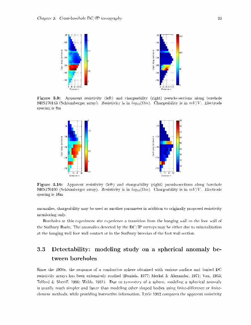
Figure 3.10 (NRS170100) recovers both in-hole and o-hole resistivity and chargeability anomalies
at various resistivity-chargeability combinations while NRS170162 (Figure 3.11) mainly intersect a low
resistivity and high chargeability anomaly which extends away from the borehole. Tomography results
recovers similar anomalies (Figure 3.12). However, it is noted that these anomalies are associated
with individual boreholes rather than connected across the two boreholes. The middle area has small
variation in both resistivity and chargeability, suggesting a relatively uniform lithology, which potentially
can be changed with mining operations. It is also suspected that as the borehole separation (more than
100m) greatly exceeds current-potential electrode spacing in each borehole (16m), the resolution between
boreholes can be too poor to recover detailed features, especially for the second half where the boreholes
are further separated. The resistivity and chargeability variation may not be as uniform as suggested
in the current tomography result. As all boreholes have signicant in-hole or o-hole chargeability
Chapter 3. Cross-borehole DC/IP tomography 23
Figure 3.9: Apparent resistivity (left) and chargeability (right) pseudo-sections along boreholeNRS170143 (Schlumberger array). Resistivity is in log10(Ωm). Chargeability is in mV/V . Electrodespacing is 8m
Figure 3.10: Apparent resistivity (left) and chargeability (right) pseudo-sections along boreholeNRS170100 (Schlumberger array). Resistivity is in log10(Ωm). Chargeability is in mV/V . Electrodespacing is 16m
anomalies, chargeability may be used as another parameter in addition to originally proposed resistivity
monitoring only.
Boreholes at this experiment site experience a transition from the hanging wall to the foot wall of
the Sudbury Basin. The anomalies detected by the DC/IP surveys may be either due to mineralization
at the hanging wall-foot wall contact or in the Sudbury breccias of the foot wall section.
3.3 Detectability: modeling study on a spherical anomaly be-
tween boreholes
Since the 1930s, the response of a conductive sphere obtained with various surface and buried DC
resistivity arrays has been extensively studied (Daniels, 1977; Merkel & Alexander, 1971; Van, 1953;
Telford & Sheri, 1990; Webb, 1931). Due to symmetry of a sphere, modeling a spherical anomaly
is usually much simpler and faster than modeling other shaped bodies using nite-dierence or nite-
element methods, while providing instructive information. Lytle 1982 compares the apparent resistivity

Chapter 3. Cross-borehole DC/IP tomography 24
Figure 3.11: Apparent resistivity (left) and chargeability (right) pseudo-sections along boreholeNRS170162 (Schlumberger array). Resistivity is in log10(Ωm). Chargeability is in mV/V . Electrodespacing is 16m
Figure 3.12: (left) Resistivity tomography inversion result; (right) chargeability inversion result incommonly used RGB color scheme. Resistivity is in log10(Ωm) and chargeability is in mV/V . Thehorizontal axis is distance in the tunnel in meters. Black solid lines represent positions of boreholes wherethe measurements were taken. Borehole numbers from left to right are NRS170143 and NRS170100
Figure 3.13: Resistivity tomography in blue to green color scheme and chargeability tomography inblack to red color scheme between NRS170143 and NRS170100

Chapter 3. Cross-borehole DC/IP tomography 25
Figure 3.14: Combined resistivity and chargeability tomography result in the new 2D color schemebetween NRS170143 and NRS170100. Resistivity is in log10(Ωm) and chargeability is in mV/V
perturbation due to a conductive sphere for single- and cross-borehole surveying using a pole-pole array.
It is suggested that cross-borehole probing provides azimuth information as well as greater detectability
than single-borehole. However, the detectability of more complicated three- and four- electrode arrays
remains to be investigated.
This section rst presents the mathematical formulas of voltage response of a sphere anomaly em-
bedded in a homogeneous half-space due to low frequency injected current based on Budak et al. 1964
and Lytle 1982. The half-space and sphere can be of arbitrary resistivity. Then modelling results with
pole-dipole and dipole-dipole arrays are compared and discussed.
In the case of low frequency direct current, the electrical eld E is the gradient of potential V
E = −∇V (3.1)
By Ohm's law,
J = σE (3.2)
where σ is conductivity of the medium. Therefore,
J = −σ∇V (3.3)
For a conserved charge within a volume τ enclosed by surface S,∫S
Jda = 0 (3.4)
Then by Green's theorem ∫S
Jda =
∫V
∇Jdτ (3.5)
and at the point of this charge
∇J = −∇∇(σV ) = −(∇σ∇V + σ∇2V ) = 0 (3.6)

Chapter 3. Cross-borehole DC/IP tomography 26
Figure 3.15: Schematic plot of a sphere anomaly of radius rsph, resistivity ρ1 located between twoboreholes in a homogeneous half-space of resistivity ρ2 (adopted from Lytle., 1982). The center of thesphere is the origin of the spherical coordinate system
As a result,we get the Laplace's Equation
∇2V = 0 (3.7)
Morse and Feshbach (1953) gives the general solution for V in spherical coordinates
V (r, θ, φ) =
∞∑n=0
n∑m=0
(Amnrn +Bmnr
−n−1)Pmn (cosθ)cosmφ (3.8)
where Amn, Bmn are coecients to be determined from boundary conditions and governs potential inside
and outside the sphere respectively. Pmn (cosθ) is the associate Legendre function. Then for current source
I located outside or at the edge of the sphere (rs > rsph), the resultant potential measured at r from
the center of the sphere in spherical coordinate system (Figure 3.15)
V =Iρ24πR
+
∞∑n=1
Irsphρ24πrsr
ρ1 − ρ2(n+ 1)ρ1 + nρ2
n(r2sphrsr
)nPn(cosγ) (3.9)
and for r ≤ rsph
V =Iρ24πrs
+
∞∑n=1
Irnρ1ρ2
4πrn+1s
2n+ 1
(n+ 1)ρ1 + nρ2Pn(cosγ) (3.10)
where cosγ = cosθcosθs + sinθsinθscos(φ− φs). If the current source is inside the sphere, the resultantpotential measured inside the sphere (r < a) is calculated to be
V =Iρ14πR
+
∞∑n=0
Iρ14πrsph
(rsr
r2sph)n(ρ1 − ρ2)
n+ 1
(n+ 1)ρ1 + nρ2Pn(cosγ) (3.11)

Chapter 3. Cross-borehole DC/IP tomography 27
Figure 3.16: Apparent resistivity of the sphere model with dipole-dipole array AM − BN (left) andAM −NB (right)
and the potential measured outside the sphere (r ≥ rsph)
V =
∞∑n=0
Iρ1ρ24πr
(rsr
)n2n+ 1
(n+ 1)ρ1 + nρ2Pn(cosγ) (3.12)
For a multi-electrode arrays, the resulting potentials can be calculated by superposition of voltage
responses due to dierent current electrodes. Figure 3.16 depicts the apparent resistivity perturbation
due to a conductive sphere detected by dierent dipole-dipole cross-borehole arrays. Electrodes in each
borehole are laid from 0 to 100m at 4m spacing. The two boreholes are separated by 40m and the sphere
is placed in the middle of the boreholes at 50m. The radius of the sphere is 16m and the resistivity
contrast (ρ2/ρ1) between the sphere and the homogeneous half-space is 100 (Figure 3.15). Although
dierent in acquisition geometry, the two dierent arrays give identical apparent resistivity response as
conrmed by Figure 3.17. Similarly, dierent pole-dipole arrays gives identical response with the sphere
model (Figure 3.18). Comparing responses from dipole-dipole and pole-dipole arrays, it is found that
pole-dipole array gives greater perturbation under the same modelling parameters(Figure 3.19). The
same conclusion can be reached by setting the sphere at dierent depths. Therefore, pole-dipole array
oers greater detectability and can be a more powerful tool in detecting small perturbation such as in
tracer experiments.
Figure 3.20 depicts the total variation in apparent resistivity due to the spherical anomaly as a
function of borehole separation (d) and resistivity contrast between the sphere and the homogeneous
half-space. Compared with resistivity contrast, the borehole separation with respect to the dimension
of the sphere has a much greater impact on the detectability of the anomaly. It is found that, regardless
of resistivity contrast, the borehole separation should not exceed two times the diameter of the sphere
in order for a detectable perturbation to be detected.
3.4 Discussion
Compared with pseudo-sections from single-borehole surveys, cross-borehole DC/IP tomography pro-
vides directional constrained spatial image of resistivity and chargeability distribution between boreholes
and enables more rigorous and quantitative interpretation. However, as observed in the previous eld ex-

Chapter 3. Cross-borehole DC/IP tomography 28
Figure 3.17: Apparent resistivity perturbation due a conductive sphere between borehole with dipole-dipole array AM −BN and AM −NB. AM is xed at 50m at borehole 1 while BN or NB is shiftedalong the other borehole
Figure 3.18: Apparent resistivity perturbation due a conductive sphere between borehole with pole-dipole array AM − B and AM − N . AM is xed at 50m at borehole 1 while B or N is shifted alongthe other borehole

Chapter 3. Cross-borehole DC/IP tomography 29
Figure 3.19: Comparison of apparent resistivity along the borehole acquired with dipole-pole AM −Nand dipole-dipole AM −BN array
Figure 3.20: Percentage of variation in apparent resistivity due a spherical anomaly between boreholesat various borehole separations and resistivity contrasts

Chapter 3. Cross-borehole DC/IP tomography 30
ample at Sudbury North Range, the tomography can also be strongly aected by anomalies that are not
in the plane as what is to be imaged. Therefore, it is necessary to compare cross-borehole tomography
results with single-borehole pseudo-sections for accurate interpretation.
A 2D color scheme is proposed and it enables simultaneous display of the resistivity and charge-
ability data on the same image. With the aid of this color scheme, various combinations of resistivity-
chargeability variation can be directly visualized and be used to further dierentiate dierent lithology.
This color scheme can also be applied to display other combinations of geophysical data, such as Vp and
Vs, NMR and porosity, stress and Vp. In addition to better characterize dierent lithology, it can also
be used to show the correlation between two parameters.
Apparent resistivity perturbation due to an o-hole spherical anomaly captured by various three- and
four-electrode cross-borehole arrays are calculated and compared. Modelling results show that dipole-
dipole arrays AM −BN and AM −NB give identical response, so do pole-dipole arrays AM −B and
AM−N . Almost identical tomography results are also obtained with AM−BN and AM−NB arrays in
a eld experiment at Canadian Malartic Mine (Chapter 4). Moreover, for the same anomaly, pole-dipole
arrays generally capture greater perturbation than dipole-dipole arrays. Thus, in eld experiment, pole-
dipole arrays oer better signal strength and are more recommended for geotechnical and environmental
monitoring surveys where there is little noise for the innite electrode. In addition, it is found that the
detectability of cross-borehole measurements is primarily determined by borehole separation rather than
resistivity contrast. In order to get eective response from the target in the middle of the boreholes, the
borehole separation should not be more than two times greater than the dimension of the target.

Chapter 4
Towards 3D
As geological features are three dimensional, potential targets can only be fully recovered by 3D DC/IP
surveys. Conventional 3D DC/IP surveys adopt a layout of square or rectangular electrode grid on the
surface and measurements are taken at various current-potential electrode combinations (Loke, 2001).
However, such 3D surveys have not become commonly practice for either exploration or monitoring as
they require a large number of electrodes and measurements and therefore are not economic nor time
ecient. In addition, similar to 2D surface DC/IP surveys, the data resolution decreases exponentially
with depth (Oldenburg & Li, 1999). However, with the availability of boreholes, surface-to-borehole and
cross-borehole measurements can be taken in addition to surface measurements. This can potentially
greatly reduce the number of electrodes required on the surface while providing depth constrained tomog-
raphy results. A combination of cross-borehole, surface-to-surface, surface-to-borehole DC/IP surveys
were conducted at an exploration site of Canadian Malartic Mine. Three boreholes and three surface
lines were used and measurements were taken at various cross-borehole, surface-to-borehole and surface-
to-surface combinations (Figure 4.1). The three boreholes are approximately 100m apart with similar
dip and azimuth. The three surface lines start from the borehole collars and run at similar azimuths
as the boreholes. Previous surface mapping and geophysicald surveys have identied gold deposits and
near surface IP anomalies. The goal of this eld experiment is to better delineate the distribution of
gold deposits at depth and to investigate the 3D DC/IP imaging capability with combinations of pro-
posed acquisition geometry. Unless specied, tomography data were acquired with dipole-dipole array
AM − BN . One of the cross-borehole surveys was also conducted with another dipole-dipole array
AM −NB to compare the detectability of the two arrays.
4.1 Single surface lines
The three surface lines are all 124m in length using 4m electrode spacing. The measurements were
taken with Schlumberger array and the apparent resistivity and chargeability pseudo-sections are shown
from Figure 4.2 to 4.4. Figure 4.5 gives waveforms examples of injection current and voltage response
with and without IP or other distortion eects measured in L3 survey. Pseudo-sections of L1 and L2
show similar resistivity and chargeability patterns. Two vertical bands of low resistivity anomalies occur
in the rst half of the lines, in which the location of the rst band in L2 coincides with an outcrop
containing low grade gold mineralization. The chargeability increases with increasing current-potential
31
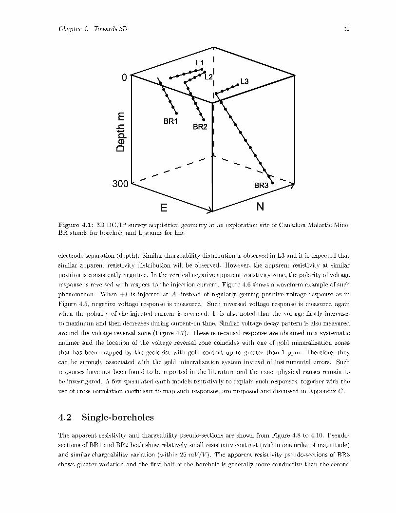
Chapter 4. Towards 3D 32
Figure 4.1: 3D DC/IP survey acquisition geometry at an exploration site of Canadian Malartic Mine.BR stands for borehole and L stands for line
electrode separation (depth). Similar chargeability distribution is observed in L3 and it is expected that
similar apparent resistivity distribution will be observed. However, the apparent resistivity at similar
position is consistently negative. In the vertical negative apparent resistivity zone, the polarity of voltage
response is reversed with respect to the injection current. Figure 4.6 shows a waveform example of such
phenomenon. When +I is injected at A, instead of regularly getting positive voltage response as in
Figure 4.5, negative voltage response is measured. Such reversed voltage response is measured again
when the polarity of the injected current is reversed. It is also noted that the voltage rstly increases
to maximum and then decreases during current-on time. Similar voltage decay pattern is also measured
around the voltage reversal zone (Figure 4.7). These non-causal response are obtained in a systematic
manner and the location of the voltage reversal zone coincides with one of gold mineralization zones
that has been mapped by the geologist with gold content up to greater than 1 ppm. Therefore, they
can be strongly associated with the gold mineralization system instead of instrumental errors. Such
responses have not been found to be reported in the literature and the exact physical causes remain to
be investigated. A few speculated earth models tentatively to explain such responses, together with the
use of cross-correlation coecient to map such responses, are proposed and discussed in Appendix C.
4.2 Single-boreholes
The apparent resistivity and chargeability pseudo-sections are shown from Figure 4.8 to 4.10. Pseudo-
sections of BR1 and BR2 both show relatively small resistivity contrast (within one order of magnitude)
and similar chargeability variation (within 25 mV/V ). The apparent resistivity pseudo-sections of BR3
shows greater variation and the rst half of the borehole is generally more conductive than the second

Chapter 4. Towards 3D 33
Figure 4.2: Apparent resistivity (left) and chargeability (right) pseudo-section of L1 (Schlumbergerarray). Resistivity is in log10(Ωm). Chargeability is in mV/V . Electrode spacing is 4m
Figure 4.3: Apparent resistivity (left) and chargeability (right) pseudo-section of L2 (Schlumbergerarray). Resistivity is in log10(Ωm). Chargeability is in mV/V . Electrode spacing is 4m
Figure 4.4: Apparent resistivity (left) and chargeability (right) pseudo-section of L3 (Schlumbergerarray). Resistivity is in log10(Ωm). Chargeability is in mV/V . Electrode spacing is 4m

Chapter 4. Towards 3D 34
Figure 4.5: Waveform examples from L3 of injection current and voltage response without (left) andwith (right) IP and other distortion eects from L3
Figure 4.6: Waveforms of injection current and reversed voltage response with IP eect from voltagereversal zone at 50m of L3

Chapter 4. Towards 3D 35
Figure 4.7: Waveforms of injection current and voltage response with IP eect of reversed polarity
Figure 4.8: Apparent resistivity (left) and chargeability (right) pseudo-section along BR1 (Schlum-berger array). Resistivity is in log10(Ωm). Chargeability is in mV/V . Electrode spacing is 8m
half. The chargeability pseudo-section of BR3 shows two strongly chargeable zones at about 120m and
180m along the borehole, in which the 120m one locates at similar location as previously discussed
voltage reversal zone (4.6). The two anomalies can be responses from the same lithology.
4.3 Cross-boreholes
Cross-BR1-BR2 resistivity and chargeability tomography are shown in Figure 4.11 and 4.12. The resis-
tivity tomography recovers a conductive anomaly between BR1 and BR2 and the anomaly extends to
BR2. Also, BR1 gets into conductive materials at the end the borehole. These features are also sug-
gested by single-borehole surveys (Figure 4.8, 4.9). However, cross-borehole tomography provides more
information on the spatial distribution of dierent anomalies. The chargeability tomography suggests
that the materials between BR1 and BR2 have a small chargeability variation while lithology around
the middle of BR1 is more chargeable than that of around BR2. This feature is not captured by the

Chapter 4. Towards 3D 36
Figure 4.9: Apparent resistivity (left) and chargeability (right) pseudo-section along BR2 (Schlum-berger array). Resistivity is in log10(Ωm). Chargeability is in mV/V . Electrode spacing is 8m
Figure 4.10: Apparent resistivity (left) and chargeability (right) pseudo-section along BR3 (Schlum-berger array). Resistivity is in log10(Ωm). Chargeability is in mV/V . Electrode spacing is 16m

Chapter 4. Towards 3D 37
Figure 4.11: Resistivity tomography betweenBR1(Left) and BR2(right) in log10(Ωm). Elec-trode spacing is 8m
Figure 4.12: Chargeability tomography be-tween BR1(Left) and BR2(right) in mV/V .Electrode spacing is 8m
Figure 4.13: Resistivity tomography betweenBR1(Left) and BR2(right) in log10(Ωm). Datais acquired with dipole-dipole array AM−NB.Electrode spacing is 8m
Figure 4.14: Chargeability tomography be-tween BR1(Left) and BR2(right) in mV/V .Data is acquired with dipole-dipole array AM−NB. Electrode spacing is 8m
single-borehole measurement.
BR1-BR2 tomography data were also collected with another type of dipole-dipole array AM−NB, inwhich the positions of current and potential electrodes in the second borehole are switched. The results
are shown in Figure 4.13 and 4.14. Although with anisotropy of earth materials and potential noise in
the eld measurement, the resistivity tomography result from AM − NB array gives almost identical
resistivity distribution pattern as that of from AM − BN array with slightly dierence in amplitude.
This conrms the modelling result from the previous chapter. However, the chargeability tomography
shows a rather dierent chargeability distribution. It is suggested that, instead of BR1, BR2 experience
more chargeable lithology in the middle of the borehole. Similar feature is also noted by comparing
single-borehole chargeability pseudo-sections of the two boreholes. This suggests that the AM − NBarray may be a more reliable array in imaging chargeability distribution while provide similar resistivity
results as the AM −BN array.
Tomography results between BR1 and BR3 (Figure 4.15, 4.16) show a conductive anomaly at the
end of BR2, a chargeable anomaly between the end of BR1 and BR2 and another one around the top

Chapter 4. Towards 3D 38
Figure 4.15: Resistivity tomography betweenBR1(Left) and BR3(right most) in log10(Ωm).BR2 is also plotted for reference. Electrodespacing is 16m. BR3 is the edge of the imageat 200m
Figure 4.16: Chargeability tomography be-tween BR1(Left) and BR3(right most) inmV/V . BR2 is also plotted for reference. Elec-trode spacing is 16m. BR3 is the edge of theimage at 200m
of BR3. However, both resistivity and chargeability tomography fail to recover the details between BR1
and BR2 as in the BR1-BR2 tomography(Figure 4.11, 4.14). Moreover, it shows no coincidence with
resistivity and chargeability anomalies observed in pseudo-sections along BR1 and BR3 (Figure 4.8 and
4.10). Referring to Figure 3.20, it is speculated that, compared with borehole separation, the dimensions
of anomalies between BR1 and BR3 is too small to be delineated by cross-borehole array AM −BN .
4.4 Surface-to-surface
Similar as cross-borehole measurement, the AM−BN array was also applied between surface lines. The
data is inverted in the same way as cross-borehole data though a half-space geometry factor is used in
calculating the apparent resistivity. The results are shown from Figure 4.17 and 4.20. In Figure 4.17,
two conductive bands across L1 and L2 are observed. This coincides with the two conductive bands in
the pseudo-sections of L1 and L2 and suggests that each of the two bands are connected across L1 and
L2. Chargebility tomography suggests a chargeable zone between the end of L1 and L2. This result
shows that array AM −BN is applicable to surface lines and is capable of near surface tomography at
proper line separation. It is useful in mapping the connectedness of near surface anomalies. However,
the depth of investigation remains to be investigated.
For cross-L1-L3 tomography measured at a greater separation, resistivity and chargeability tomog-
raphy both only show anomalies associated with each line with little detail in between. Also, it fails to
recover details between L1 and L2 as observed in the L1-L2 tomography (Figure 4.19, 4.18). Similar as
the case of BR1-BR3 tomography, the missing of details is likely because the size of anomalies is too
small comparing with the separation between L1 and L3.
4.5 3D reconstruction
Figure 4.21 gives a 3D reconstruction of resistivity and chargeability distribution with surface-to-surface,
cross-borehole tomography and surface line pseudo-sections. It clearly shows that each the two conduc-
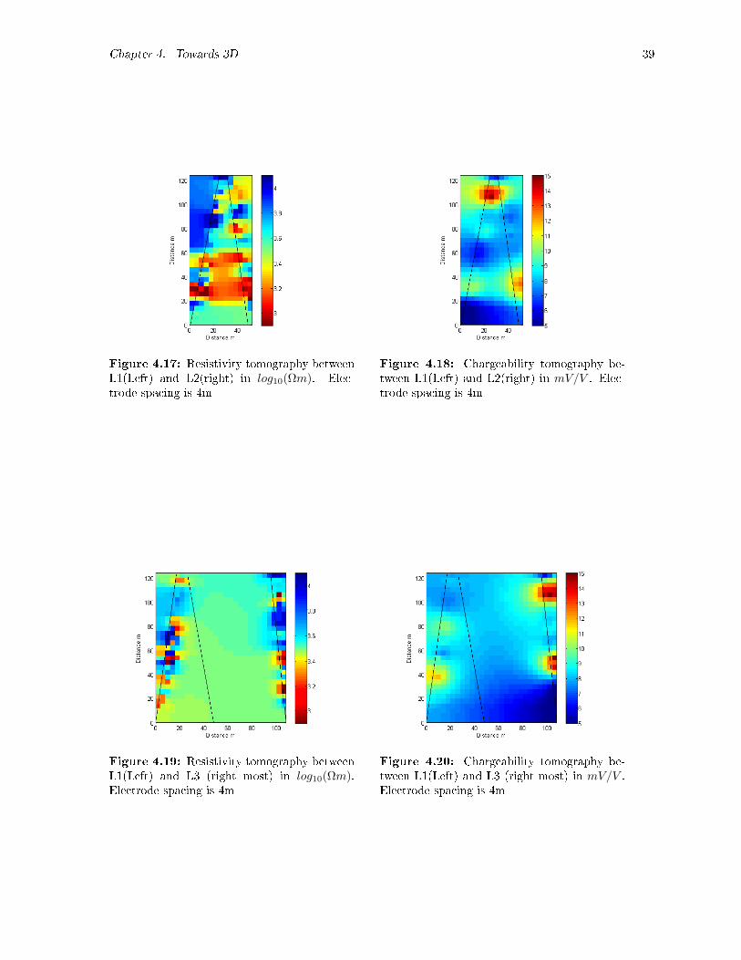
Chapter 4. Towards 3D 39
Figure 4.17: Resistivity tomography betweenL1(Left) and L2(right) in log10(Ωm). Elec-trode spacing is 4m
Figure 4.18: Chargeability tomography be-tween L1(Left) and L2(right) in mV/V . Elec-trode spacing is 4m
Figure 4.19: Resistivity tomography betweenL1(Left) and L3 (right most) in log10(Ωm).Electrode spacing is 4m
Figure 4.20: Chargeability tomography be-tween L1(Left) and L3 (right most) in mV/V .Electrode spacing is 4m
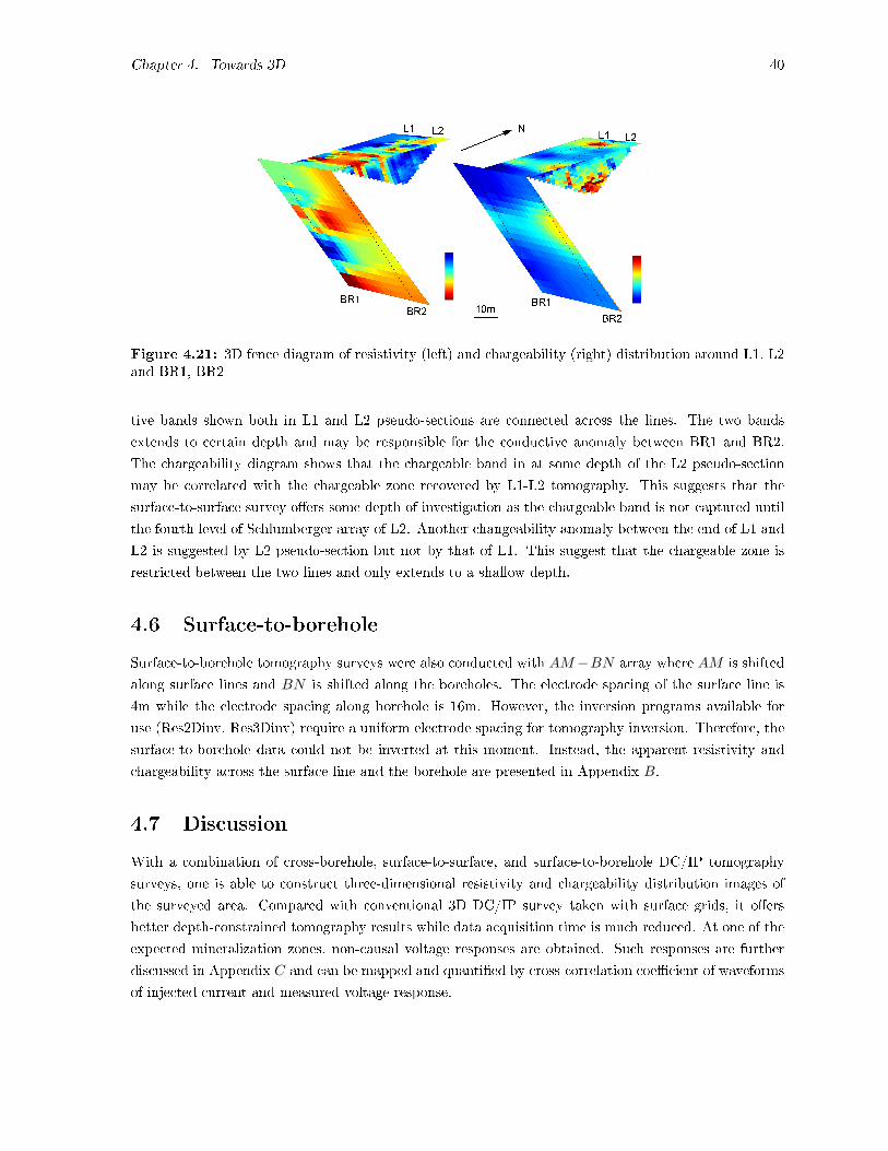
Chapter 4. Towards 3D 40
Figure 4.21: 3D fence diagram of resistivity (left) and chargeability (right) distribution around L1, L2and BR1, BR2
tive bands shown both in L1 and L2 pseudo-sections are connected across the lines. The two bands
extends to certain depth and may be responsible for the conductive anomaly between BR1 and BR2.
The chargeability diagram shows that the chargeable band in at some depth of the L2 pseudo-section
may be correlated with the chargeable zone recovered by L1-L2 tomography. This suggests that the
surface-to-surface survey oers some depth of investigation as the chargeable band is not captured until
the fourth level of Schlumberger array of L2. Another changeability anomaly between the end of L1 and
L2 is suggested by L2 pseudo-section but not by that of L1. This suggest that the chargeable zone is
restricted between the two lines and only extends to a shallow depth.
4.6 Surface-to-borehole
Surface-to-borehole tomography surveys were also conducted with AM −BN array where AM is shifted
along surface lines and BN is shifted along the boreholes. The electrode spacing of the surface line is
4m while the electrode spacing along borehole is 16m. However, the inversion programs available for
use (Res2Dinv, Res3Dinv) require a uniform electrode spacing for tomography inversion. Therefore, the
surface-to-borehole data could not be inverted at this moment. Instead, the apparent resistivity and
chargeability across the surface line and the borehole are presented in Appendix B.
4.7 Discussion
With a combination of cross-borehole, surface-to-surface, and surface-to-borehole DC/IP tomography
surveys, one is able to construct three-dimensional resistivity and chargeability distribution images of
the surveyed area. Compared with conventional 3D DC/IP survey taken with surface grids, it oers
better depth-constrained tomography results while data acquisition time is much reduced. At one of the
expected mineralization zones, non-causal voltage responses are obtained. Such responses are further
discussed in Appendix C and can be mapped and quantied by cross-correlation coecient of waveforms
of injected current and measured voltage response.

Chapter 4. Towards 3D 41
Figure 4.22: 3D view of various anomaly distrition with respect to the acquistion conguration
Chapter 5
Discussion and Conclusions
The DC resistivity and induced polarization responses of earth materials are not only determined by
the electrical properties of the lithology, but are strongly inuenced by presence of stress, pore space
and uid contents. As measurements taken in boreholes provide good repeatability over conventional
surface arrays, borehole DC/IP imaging can be a powerful tool for monitoring time lapse changes in
geotechnical and environmental studies. Also, for DC/IP surveys taken for mineral exploration purposes
under a stressed environment, extra care should be taken in interpretation as the anomaly may be also
due to stress anomaly or uid lled structures.
For near surface borehole DC/IP surveys, the geometry factor plays an important role in accounting
for the deviation eect and transition from half-space to full-space as the electrode array is shifted from
the top to the bottom of the borehole. It is found that deviation and transition eects are both depth
and dipping angle dependent. They are especially important for shallow dipping boreholes, in which
case the dierence in apparent resistivity calculated with and without correct geometry factors remains
above typical data noise level throughout the boreholes. Such dierence can be problematic in accurately
imaging potential target structures. Therefore, for near surface borehole DC/IP surveys, rather than
assuming a vertical borehole and/or full-space setting, the exact locations of electrode arrays should be
obtained so that correct geometry factors can be applied for apparent resistivity calculation. Moreover,
for cross-borehole DC/IP surveys, the geometry factor of certain array conguration may behave near
singularly when the borehole separation is smaller than the current-potential electrode spacing. Data
obtained with such arrays should be avoided in order to avoid introducing artifacts in tomography
inversion. Alternatively, dipole-dipole array AM −NB can be used. It oers similar detectability and
its geometry factor is free of singularity issue. For current electrodes A and B in separate boreholes, the
maximum of horizontal eld is reached when the current-potential electrode separation is√
2 times the
borehole separation, at which the target can be best detected.
For underwater DC/IP surveys, a modied geometry factor is proposed to account for presence
of the water layer. At the water-earth interface, more currents tend to ow into the water layer as
the water is usually less resistive than sediments. However, with presence of conductive materials in
the sediments such as clays and iron oxides, current may also tends to ow in the sediments side. The
modied geometry factor requires estimates of resistivity of the water as well as the underlying half-space
and is simple to be programmed for apparent resistivity calculation. It has been applied to resistivity
data acquired with underwater conguration, where the water is more conductive than the sediments
42

Chapter 5. Discussion and Conclusions 43
and tends to bring down overall apparent resistivity. It eectively removes the low resistivity layer on
the top of the pseudo-section, which is mostly aected by the water layer. Moreover, for time lapse
DC/IP monitoring surveys associated with water, the temperature-resistivity variation of water also has
a strong impact on resistivity data and should be well accounted. By applying dierent temperature-
conductivity relationships reported in the literature to repeated resistivity measurements taken in the
summer and the winter, the simple linear temperature-conductivity relationship is found to be more
eective in temperature correction than the viscosity-based relationship (Appendix A).
Compared with single-borehole DC/IP surveys, cross-borehole DC/IP tomography provides direc-
tional and depth constrained spatial image of resistivity and chargeability distribution between boreholes.
It greatly assists more rigorous and quantitative interpretation than using curving tting and pseudo-
sections. As geological features are three dimensional, cross-borehole DC/IP tomography is not only
imaging the electrical properties in the plane of the boreholes, but may also be strongly inuenced
by o-hole targets. Cross-borehole tomography with surface boreholes at Sudbury North Range suggest
that all three boreholes intersect a chargeability anomaly. However, after comparing with single-borehole
pseudo-sections, it is concluded that the anomaly is likely to be due to an o-hole target. Therefore, al-
though cross-borehole tomography has the advantage of providing 2D spatial distribution of imaged area,
it should be combined with single-borehole surveys for accurate interpretation. In addition, environmen-
tal monitoring surveys, such as tracer experiments, are generally not recommended to be conducted
close to background anomalies. The responses from tracer may manifest with background anomalies
even though the anomalies are not in the same plane to be imaged.
A 2D color scheme is proposed for DC/IP tomography display. Using this color scheme, resistivity
and chargeability data can be displayed on the same image and lithology associated with dierent
resistivity-chargeability combinations can be directly dierentiated by dierent colors in the color scheme.
Rather than comparing two sets of data side by side, it enables direct visual examination of resistivity-
chargeability variation pattern of the imaged area. This new color scheme can also be used to display
other geophysical data, such as Vp and Vs, NMR and porosity, stress and Vp, to better characterize
lithological changes and to investigate the correlation between two parameters.
Modeling results are calculated with dierent cross-borehole arrays for a conductive sphere between
boreholes. It is shown that, although dierent in acquisition geometry, dipole-dipole arrays AM − BNand AM−NB give identical apparent resistivity responses. This modeling results is conrmed by cross-
borehole resistivity tomography results from the exploration site at Canadian Malartic Mine, although
with anisotropy of the Earth materials and potential noise in the eld measurements. However, the two
arrays give dierent chargeabilty tomography results across the same area. Considering the electrode
separation is 16m at each measurement, the dierence in chargeability tomography may be due to the
fact that the current electrodes of one of the two arrays happen to have more contact with dierent parts
of chargeable materials. With the sphere model, identical responses are also obtained with dipole-pole
arrays AM − B and AM − N . Moreover, dipole-pole arrays generally oer greater detectability than
dipole-dipole arrays. Therefore, in case of small background noise for remote electrode, pole-dipole array
is recommended for geotechnical and environmental monitoring surveys. It is also found that, for an
o-hole anomaly, it is the borehole separation with respect to the dimension of the anomaly, rather than
the resistivity contrast between the anomaly and the homogeneous half-space that plays the primary
role that determines the detectability of the anomaly. In general, one should not expect to get eective
responses from the anomaly in the middle of the two boreholes when the borehole separation is more

Chapter 5. Discussion and Conclusions 44
than two times greater than the dimension of the anomaly.
A combination of cross-borehole, surface-to-surface, and surface-to-borehole DC/IP were conducted
at an exploration site of Canadian Malartic Mine in order to construct three-dimensional images of
resistivity and chargeability distributions and to give DC/IP characterization of a gold mineralization
system. At one of the expected mineralization zones, various non-causal voltage responses are obtained
in a systematic manner, including voltage discharge while the current is being injected, voltage and
induced polarization responses with reversed polarization. Such responses are obtained around the same
expected mineralization zone and thus are unlikely to be due to instrumental errors. Some models have
been proposed to explain such non-causal responses (Appendix C). However, the exact physical causes
or complexity introduced by 3D heterogeneity of geology remain to be investigated.
Comparing with conventional 3D DC/IP surveys taken with surface grid, cross-borehole and surface-
to-borehole surveys provide better depth constraint imaging while reducing data acquisition time. In
addition, with presence of near surface anomalies, surface-to-surface tomography is found to be a use-
ful tool to map the connectedness of these near surface anomalies. Due to limitation of inversion
algorithm currently available, the surface-to-borehole dataset cannot be inverted. However, 3D resis-
tivity and chargeability distribution images are able to be constructed by combining surface-to-surface,
cross-borehole tomography results and surface line pseudo-sections. In addition to delineating a known
mineralization zones with surface expressions, several anomalies are identied as potential mineralization
zones.

Chapter 6
Outlook/Recommendations
Based on numerical modeling and eld experiment results, the following actions and recommendations
are proposed
1. Repeated single-borehole DC/IP measurement will be conducted on both 1300 and 1700 levels at
the deep mine at Sudbury East Range. The correlation between potential changes in resistivity
and stress will be investigated. In addition, the applicability of induced polarization eect in time
lapse monitoring under a stressed environment will be discussed.
2. Cross-borehole DC/IP surveys will be taken with surface boreholes at Sudbury North Range at
dierent osets. The detectability and changes in resolution of DC/IP tomography at dierent
borehole separation will be examined.
3. More sophisticated inversion algorithms are required to invert surface-to-borehole data taken at the
exploration site of Canadian Malartic Mine. Then more complete 3D resistivity and chargeability
images can be obtained across the surveyed area. The DC/IP results will also be combined with
geological information to give geophysical and geological characterization of the gold mineralization
system at Canadian Malartic Mine.
4. More research, both numerical modeling and laboratory experiment, is recommended to better
understand the physical causes of voltage and IP response with reversed polarity as observed in
the measurements at the exploration site of Canadian Malartic Mine.
5. DC/IP measurements on cores samples are required to give the DC/IP characterization of dif-
ferent lithology. Then single-borehole and cross-borehole imaging results can be more accurately
interpretative in terms of real geology.
45

Appendices
46

Appendix A
Tempertature-electrical resistivity
correction for water related DC
resistivity monitoring
The electrical conductivity of water is controlled by the combination of total dissolved solid and the
temperature (Chang et al., 1983; Millero, 2001). The general conductivity-temperature relationship is
complicated and non-linear (Millero, 2001). However, in the range of 0 to 30 C for environmental mon-
itoring, a linear and a viscosity-based equations are commonly used to represent the relation (Sorensen
& Glass, 1987)
σ(t) = σ(25)[1 + ε(t− 25)] (A.1)
where σ(t) is electrical conductivity at temperature t in C; ε is temperature compensation factor and
is recommended to be 0.0187 for natural waters (Hayashi, 2004).
σ(t) = σ(25)(µt/µ25)−b (A.2)
where log µt
µ25= A(25−t)−B(25−t)2
t+C , ut is viscosity of water at temperature t C, µ25 = 0.0008903Nsm−2,
A = 1.1278, B = 0.001895 C−1, C = 88.93 C (Hayashi, 2004; Korson et al., 1969). Then the electrical
resistivity is simply the inverse of electrical conductivity.
The percentage of change relative to resistivity at 0 C based on Equation A.1 and A.2 is depicted in
Figure A.1. In general, resistivity of water decreases with increasing temperature. However, Equation
A.1 suggests a higher degree of variation compared with that of suggested by Equation A.2.
On Ogilvie's lake, Deep River, Ontario, repeated DC resistivity surveys across the lake have been
conducted both in the summer and winter. The water layer is about 2m in thickness and has a signicant
impact on the rst few levels of the data as the electrode spacing is 4m. In the winter, holes were drilled
on the frozen lake so that electrodes could be put in contact with lake water. The change in resistivity
inversion results due to change in resistivity of water can be clearly observed in Figure A.2. The
inversion results of data collected in the winter collaboratively unveil a relatively resistive top layer,
which is primarily caused by decrease in temperature of lake water.
47

Appendix A. Tempertature-electrical resistivity correction for water related DC resistivity monitoring48
Figure A.1: Percentage of change in electrical resistivity from 0 to 30 C based on Equation A.1 andA.2
Figure A.2: Inverted resistivity pseudo-section of line 4 on Ogilvie's lake in the summer (top) and inthe winter(bottom). The array type is Schlumberger and electrode spacing is 4m

Appendix A. Tempertature-electrical resistivity correction for water related DC resistivity monitoring49
Figure A.3: Modied inverted resistivity pseudo-section of line 4 on Ogivile's lake in the winter basedon Equation A.1 (top) and A.2 (bottom)
.
Equation A.1 and A.2 are both used to correct for temperature-resistivity variation of water. From
0C to 25 C, the percentage of change is 47% and 24% respectively. The modied results are shown
in Figure A.3. By visual inspection, the top 5m in the modied resistivity pseudo-section using Equa-
tion A.1 is more uniform than that of using Equation A.2. Previous researchers have suggested that
the conductivity-temperature relation is primarily controlled by change in viscosity of water and the
viscosity-based equation should oers a higher accuracy than the linear relation(Robinson & Stokes,
1965; Korson et al., 1969; Sorensen & Glass, 1987; Hayashi, 2004). However, application of both equa-
tions to DC resistivity eld examples on Ogilvie's lake suggests that Equation A.1 is more eective in
correcting temperature based resistivity variation.

Appendix B
Surface-to-borehole
Due to limitation of the inversion program currently available for use (Res2Dinv, Res3Dinv), the surface-
to-borehole tomography data from the exploration site at Canadian Malartic Mine could not be inverted.
Instead, the apparent resistivity and chargeability across the surface line and the borehole are presented
and discussed below. The distances along the two axes are the positions of the middle of AM or BN .
All surface-to-borehole tomography surveys were also conducted with AM − BN array where AM is
shifted along surface lines and BN is shifted along the boreholes. The electrode spacing of the surface
line is 4m while the electrode spacing along borehole is 16m. The distances along the two axes are the
positions of the middle of AM or BN .
The L1-to-BR1 apparent resistivity result shows two conductive zones when AM is at around 20m,
50m and the two zones remains conductive and the one at 20m gets more chargeable as BN is shifted
along BR1. This conrms the previous conclusion that the two conductive bands, shall extend towards
BR1. A third conductive zone is shown at around 100m of L1. This is also a chargeable zone which
extends along BR1. Similar features can be observed in the L2-to-BR1 survey. The apparent resistivity
of L2-to-BR1 clearly shows the three conductive zones while the distances along L2 are consistently
being shifted by about 10m. It shows that of conductive zone at 30m at L2 end is more chargeable than
that of at the L1 end while the the conductive zone at 110m is less chargeable.
However, similar features are not observed in results from L2-to-BR2 or L1-to-BR2 surveys. As a
matter of facts. it seems that both the resistivity and chargeability data is strongly contaminated by
noise.
The L1-to-BR3 survey again shows three conductive zones at around 30m, 60m and 100m of L1 and
these zones, remains conductive while BN is being shifted along BR3. However, the 30m and 100m zones,
especially the 100m one, become much less conductive than the 60m. However, it is suggested that the
60m zone is associated with low chargeability while the 100m zone is associate with high chargeability.
These two zones may both be mineralization zones however are associated with dierent lithology and/or
dierent in concentration. Similar features are also observed in L3-to-BR3 survey and are likely to be
caused by same mineralization as in previous mentioned surface-to-borehole surveys. However, the 30m
zone becomes mostly non-chargeable and 60m zone does not start until BN is at 100m along BR3. This
suggests that, from west to east, the the mineralization becomes less chargeable and the top gets deeper
into the Earth.
50

Appendix B. Surface-to-borehole 51
Figure B.1: Apparent resistivity along L1 andBR1 in log10(Ωm)
Figure B.2: Chargeability along L1 and BR1in mV/V
Figure B.3: Apparent resistivity along L2 andBR2 in log10(Ωm)
Figure B.4: Chargeability along L2 and BR2in mV/V
Figure B.5: Apparent resistivity along L1 andBR2 in log10(Ωm)
Figure B.6: Chargeability along L1 and BR2in mV/V

Appendix B. Surface-to-borehole 52
Figure B.7: Apparent resistivity along L2 andBR1 in log10(Ωm)
Figure B.8: Chargeability along L2 and BR1in mV/V
Figure B.9: Apparent resistivity along L3 andBR3 log10(Ωm)
Figure B.10: Chargeability along L3 andBR3 in mV/V
Figure B.11: Apparent resistivity along L1and BR3 log10(Ωm)
Figure B.12: Chargeability along L1 andBR3 in mV/V

Appendix C
Suggested models for non-causal
voltage responses
In the DC/IP survey along surface line L3 at the exploration site of Canadian Malartic Mine, voltage
and IP responses with reversed polarity were obtained as seen in Figure 4.6, 4.7. These responses are
measured systematically from one of the expected mineralization zones that has been mapped by the
geologists and are unlikely to be due to instrumental errors. As illustrated in Figure C.1 a, for a AMNB
array in a homogeneous full-space, the potential from M to N decreases when current is injected at A.
Then ∆V = VM − VN has the same polarity as current injection at A. If the material is chargeable,
∆V rstly keeps increasing during current-on time and then decays back to 0 during current-o time.
However, in the vertical negative apparent resistivity zone, it is found that the polarity of voltage
response is reversed with respect to the injection current. Figure 4.6 shows a waveform example of such
phenomenon. When +I is injected at A, instead of getting positive response as in Figure 4.5, negative
voltage response is measured. Such reversed voltage response is measured again when current is injected
at B. One possible explanation for such non-causal phenomenon is illustrated in Figure C.1 b. Due to
disturbance of conductive materials, when +I is injected at A, potential at N is higher than potential
at M and therefore negative ∆V is measured. Another possibility is illustrated in Figure C.2. In a 3D
Earth, the injected current initially ows at some azimuth with respect to the prole being measured.
Then it ows in a circular pattern towards the prole through some chargeable materials (simplied as
a capacitor) and nally sinks at the other current electrode. Then negative voltage response will be
measured at one side the of current ow circle. Also, when the current is switched o, the capacitor acts
as a current source. The current ows in a regular pattern so that IP eect with a opposite polarity with
respect to the on-time voltage response is obtained. It is also noted that the voltage rstly increases to
maximum and then decreases during current-on time. Similar voltage decay pattern is also measured
around the voltage reversal zone (Figure 4.7). One possible layered Earth model responsible for such
phenomenon is illustrated in Figure C.3. The rst layer of the Earth is represented as a capacitor and
the following layers as resistors in parallel with the capacitor. The injected current rst ows through
the capacitor so that the voltage response increases. Then, the current ows into subsequent layers
which act as resistors. For a parallel conguration, the current tends to ow through resistors rather
than the capacitor and, by Ohm′s law, the measured voltage decreases. However, the exact cause also
remains to be investigated.
53

Appendix C. Suggested models for non-causal voltage responses 54
Figure C.1: Schematic plots of equipotentials (dashed lines) of array AMNB. a(top) in a homogeneousfull-space; b(bottom) disturbed by resistivity anomaly and give reversed voltage response
The cross-correlation coecient at zero time lag of the current and voltage waveforms Φ(τ = 0)
can be used to quantify such distortion eects. Without IP and other distortion eects, Φ is close
to 1. Its deviation from 1 indicates the degree of distortion of the voltage response from the injected
current. As depicted in Figure C.5, the Φ pseudo-section clearly recovers the chargeability anomalies as
in Figure C.4. However, in case of NRS170100 where the chargeability anomaly does not coincide with
the resistivity anomaly, the Φ pseudo-section gives slightly dierent anomaly distribution pattern from
either the apparent resistivity or chargeability pseudo-sections. For L3 survey, Φ gets close to -1 in the
voltage reversal zone. Also, it recovers the chargeability anomaly at the bottom of the pseudo-section.
One advantage of using the Φ parameter over chargeability is that it is less aected by presence of
self-potential. However, the quantitative relationship between Φ and the other two parameters remains
to be established.

Appendix C. Suggested models for non-causal voltage responses 55
Figure C.2: Schematic plots of a capacitor with reversed current ow in a 3D Earth
Figure C.3: Simplied circuit digram representing the layered Earth materials as a capacitor in parallelwith resistors
Figure C.4: Apparent resistivity in log10(Ωm)(left), chargeability in mV/V (right) pseudo-sections ofNRS170143

Appendix C. Suggested models for non-causal voltage responses 56
Figure C.5: Cross-correlation coecient pseudo-section of NRS170143
Figure C.6: Apparent resistivity in log10(Ωm) (left), chargeability in mV/V (right) pseudo-sections ofNRS170100

Appendix C. Suggested models for non-causal voltage responses 57
Figure C.7: Cross-correlation coecient pseudo-section of NRS170100
Figure C.8: Apparent resistivity in log10(Ωm) (left), chargeability in mV/V (right) pseudo-sections ofL3
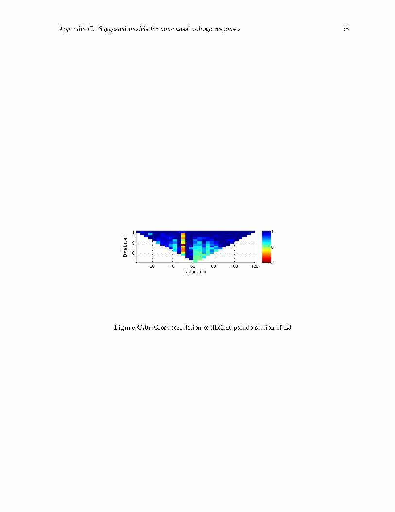
Appendix C. Suggested models for non-causal voltage responses 58
Figure C.9: Cross-correlation coecient pseudo-section of L3

Bibliography
Archie, G, E., 1942, The electrical resistivity log as an aid in determining some reservoir characteristics,
Petroleum Transactions of AIME , 146, 5462.
Asch, T. & Morrison, H. F., 1989, Mapping and monitoring electrical resistivity with surface and sub-
surface electrode arrays, Geophysics, 54(2), 235244.
Asfahani, J., 2005, Directional borehole logging congurations using dc and telluric methods for detecting
deep conductors not intersected by wells, Pure and Applied Geophysics, 162(12), 25232556.
Baumgartner, F., 1996, A new method for geoelectrical investigations underwater, Geophysical Prospect-
ing , 44(1), 7198.
Bevc, D. & Morrison, H. F., 1991, Borehole-to-surface electrical resistivity monitoring of a salt water
injection experiment, Geophysics, 56(6), 769777.
Binley, A. & Kemna, A., 2005, Dc resistivity and induced polarization methods, in Hydrogeophysics. Wa-
ter and Science Technology Library 50 , edited by R. Yuram & S. Hubbard, pp. 129156, Springer,New
York, USA.
Bleil, D., 1953, Induced polarization, a method of geophysical prospecting, Geophysics, 18(3), 636661.
Brace, W. F. & Orange, A., 1968a, Electrical resistivity changes in saturated rocks during fracture and
frictional sliding, Journal of Geophysical Research, 73(4), 14331445.
Brace, W. F. & Orange, A., 1968b, Further studies of the eects of pressure on electrical resistivity of
rocks, Journal of Geophysical Research, 73(16), 54075420.
Brace, W. F., Orange, A., & Maden, T., 1965, The eect of pressure on the electrical resistivity of
water-saturated crystalline rocks, Journal of Geophysical Research, 70(22), 56695678.
Budak, B., Samarskii, A., & A.N., T., 1964, A collection of problems on Mathematical Physics, Macmil-
lan, New York, USA.
Cardarelli, E. & Filippo, G., 2009, Electrical resistivity and induced polarization tomography in in-
dentifying the plume of chlorinated hydrocardbons in sedimentary formation: a case study in rho
(milan-italy), Water Management and Research, 27, 595602.
Chang, C., Sommerfeldt, T. G., & Schaalje, G. B., 1983, Relationships of electrical conductivity with
total dissolved solid and cation concentration of sulfate-dominant soil extracts, Canadian Journal of
Soil Science, 63, 7986.
59

BIBLIOGRAPHY 60
Daily, W., Ramirez, A., Binley, A., & LaBrecque, D., 2005, Electrical resistance tomography-theory
and practice, in Near-surface geophysics, edited by D. Butler, pp. 525550, Society of Exploration
Geophysicists, Tulsa, Okla, USA.
Daniels, J., 1983, Hole-to-surface resistivity measurements, Geophysics, 48(1), 8797.
Daniels, J. & Dyck, A., 1984, Borehole resistivity and electromagnetic methods applied to mineral
exploration, IEEE Transactions on Geoscience and Remote Sensing , GE-22, 8087.
Daniels, J. J., 1977, Three-dimensional resistivity and induced polarization modelling using buried elec-
trodes, Geophysics, 42(1), 10061019.
Daniels, J. J., 1978, Interpretation of buried electrode resistivity data using a layered earth model,
Geophysics, 43(5), 9881001.
Dines, K. & Lytle, R. J., 1979, Computerized geophysical tomography, in in Proceedings of IEEE , vol. 67,
pp. 10651073.
Gallas, J. D. F., Taioli, F., & Filho, W. M., 2011, Induced polarizaiton, resistivity, and self-potential: a
case history of contamination evaluation due to landll leakage, Environmental Earth Sciences, 63(2),
251261.
Ghorban, A., Cosenza, P., Ruy, S., Doussan, C., & Florsch, N., 2008, Non-invasive monitoring of water
inltration in a silty clay loam soil using spectral induced polarization, Water Resources Research, 44,
W08402.
Glover, P., 2009, What is the cementation exponent? a new interpretation, The Leading Edge, 28(1),
8285.
Glover, P., 2010, A generalized archieâs law for n phases, Geophysics, 75(6), E247E265.
Glover, P. W., Hole, M., & Pous, J., 2000, A modied archieâs law for two conducting phases, Earth
and Planetary Science Letters, 180(3), 369383.
Hallof, P. G., Yamashita, C. M., Wynn, J. C., Grosz, A. E., Carlson-Foscz, V. L., Witherly, K. E., ., &
Reynolds, J., 1990, Induced polarization applications and case histories, SEG.
Hayashi, M., 2004, Temperature-electrical conductivity relation of water for environmental monitoring
and geophysical data inversion, Environmental monitoring and assessment , 96(1-3), 119128.
Jamtlid, A., Magnusson, K. A., Olsson, O., & Stenberg, L., 1984, Electrical borehole measurements for
the mapping of fracture zones in crystalline rock, Geoexploration, 22(3), 203216.
Kate, J. M., 1994, Shear and resistivity behaviour of sandstones, in in proceedings of the 7th IAEG
Congress, vol. 2, pp. 889897, Lisbon, Portugal.
Keller, G. & Frischknecht, F. C., 1966, Electrical Methods in Geophysics Prospecting , Pargamon Press,
Oxford.
Kemna, A., Binley, A., & Slater, L., 2004, Crosshold ip imaging for engineering and environmental
applications, Geophysics, 69(1), 97107.
BIBLIOGRAPHY 61
Kim, J. H., Yi, M. J., Park, S. G., & Kim, J. G., 2009, 4-d inversion of dc resistivity monitoring
data acquired over a dynamically changing earth model, The Journal of Physical Chemistry , 68(4),
522532.
Korson, L., Drost-Hansen, W., & Millero, F. J., 1969, Viscosity of water at various temperatures, The
Journal of Physical Chemistry , 73(1), 3439.
LaBrecque, D., Ramirez, A., Daily, W., Binley, A., & Schima, S., 1996, Ert monitoring of environmental
remediation processes, Meas. Sci. Technol., 7(375), E247E265.
Li, Y. & Oldenburg, D., 2000, 3d inversion of induced polarization data, Geophysics, 65, 19311945.
Loke, M., 2001, Tutorial: 2-d and 3-d electrical imaging surveys, Copyright (1996-2012).
Loke, M. & Barker, R., 1996a, Rapid least-squares inversion of apparent resistivity pseudosections by a
quasi-newton method, Geophysics Prospecting , 44(1), 131152.
Loke, M. & Barker, R., 1996b, Practical techniques for 3d resistivity surveys and data inversion, Geo-
physics Prospecting , 44(3), 499523.
Lytle, R., 1982, Resistivity and induced-polarization probing in the vicinity of a spherical anomaly,
Geoscience and Remote Sensing, IEEE Transactions on, GE-20(4), 493499.
Merkel, R. & Alexander, S., 1971, Resistivity analysis for models of a sphere in a half-space with buried
current source, Geophysics Prospecting , 19(4), 640651.
Millero, F., 2001, The physical chemistry of natural waters, Wiley-Interscience, New York, USA.
Morse, P. M. & Feshbach, H., 1953, Methods of Theoretical Physics, vol. Part II, New York: McGraw-
Hill.
Muller, K., Vanderborght, J., Englert, A., Kemna, A., Huisman, J. A., Rings, J., & Vereecken, H.,
2010, Imaging and characterization of solute transport during two tracer tests in a shallow aquifer
using electrical resistivity tomography and multilevel groundwater samplers,Water resources research,
46(3), E247E265.
Nimmer, R. E., Osiensky, J. L., Binley, A. M., Sprenke, K. F., & Williams, B. C., 2007, Electrical
resistivity imaging of conductive plume dilution in fractured rock, Hydrogeology Journal , 15(5), 877
890.
Olayinka, A. & Yaramanci, U., 2000, Use of block inversion in the 2-d interpretation of apparent resis-
tivity data and its comparison with smooth inversion, Journal of Applied Geophysics, 45, 6381.
Oldenborger, G., Routh, P., & Knoll, M., 2005, Sensitivity of electrical resistivity tomography data to
electrode position errors, Geophysical Journal International , 163, 19.
Oldenburg, D. & Li, Y., 1994, Inversion of induced polarization data, Geophysics, 59, 13271341.
Oldenburg, D. & Li, Y., 1999, Estimating depth of investigation in dc resistivity and ip surveys, Geo-
physics, 64(2), 403416.

BIBLIOGRAPHY 62
Oldenburg, D., McGillivary, P., & Ellis, R., 1993, Generalized subspace method for large scale inverse
problem, Geophysical Journal International , 114, 1220.
Osasan, K. S. & Afeni, T. B., 2010, Review of surface mine slope monitoring techniques, Journal of
Mining Science, 46, 177186.
Osiensky, J. L., Nimmer, R., & Binley, A. M., 2004, Borehole cylindrical noise during holeâsurface
and holeâhole resistivity measurements, Journal of Hydrology , 289(1-4), 7894.
Pun, W. & Milkereit, B., 2011, Geophysical time series data from a stressed environment , Master's
thesis, University of Toronto.
Qian, W., Milkereit, B., McDowell, G., Stevens, K., & Halladays, S., 2007, Borehole resistivity log-
ging and tomography for mineral exploration, in in Proceedings of Exploration 07: Fifth Decennial
International Conference on Mineral Exploration, edited by B. Milkereit, pp. 11151118.
Ramirez, A., Daily, W., LaBrecque, D., Owen, E., & Chestnut, D., 1993, Monitoring an underground
steam injection process using electrical resistance tomography,Water Resource Research, 29(1), 7387.
Robinson, R. & Stokes, R. H., 1965, Electrolyte solutions, Butterworth.
Schima, S., LaBrecque, D. J., & Lundegard, P. D., 1996, Monitoring air sparging using resistivity
tomography, Groundwater Monitoring and Remediation, 16(2), 131138.
Schlumberger, C., 1920, Etude sur la prospection electrique du sous-sol: Gauthier-Villar et Cie, Paris,
France.
Seigel, H. O., 1971, Some comparative geophysical case histories of base metal discoveries, Geoexplo-
ration, 9, 8197.
Seigel, H. O., Nabighian, M., Parasnis, D., & Vozo, K., 2007, The early history of the induced polar-
ization method, The Leading Edge, 26(3), 312321.
Shima, H., 1992, 2d and 3d resistivity imaging reconstruction using cross-hole data, Geophysics, 55,
682694.
Shirokova, V. L. & Ferris, F. G., 2013, Microbial diversity and biogeochemistry of a shallow pritine
canadian shield groundwater system, Geomicrobiology Journal , 30, 140149.
Slater, L. D. & Sandberg, S. K., 2000, Resistivity and induced polarization monitoring of salt transpot
under natural hydraulic gradients, Geophysics, 65(2), 408420.
Sorensen, J. A. & Glass, G. E., 1987, Ion and temperature dependence of electrical conductance for
natural waters, Analytical Chemistry , 59(13), 15941597.
Summer, J., 1976, Principle of induced polarization for geophysical exploration, Elsevier Scientic Pub.
Co.
Telford, W. M. & Sheri, R. E., 1990, Applied geophysics, vol. 1, Cambridge university press.

BIBLIOGRAPHY 63
Tsourlos, P., Ogilvy, R., Papazachos, C., & Meldrum, P., 2011, Measurement and inversion schemes
for single borehole-to-surface electrical resistivity tomography surveys, Journal of Geophysics and
Engineering , 8(4), 487.
Van, N. R., 1953, Limition on resistivity methods as inferred from the buried sphere problem, Geophysics,
18, 423433.
Van, N. R. & Cook, K. L., 1966, Interpretation of resistivity data, U.S. Government, Washington DC,
USA.
Ward, S., 1990, Resistivity and induced polarization methods, in Geotechnical and environmental geo-
physics. Society of Exploration Geophysics, vol. 1, Society of Exploration Geophysicists, Tulsa, Okla,
USA.
Webb, J., 1931, Potential due to a buried sphere, Phys.Rev.,, 37, 292302.
Yi, M., Kim, J., & Son, J., 2009, Borehole deviation eect in electrical resistivity tomography, Geo-
sciences Journal , 13(1), 87102.
Zhou, B. & Greenhalgh, S. A., 1997, A synthetic study on crosshole resistivity imaging using dierent
electrode array, Exploration Geophysics, 28, 15.
Zhou, B. & Greenhalgh, S. A., 2000, Cross-hole resistivity tomography using dierent electrode cong-
uration, Geophysical Prospecting , 48(5), 887912.
Zonge, K., Wynn, J., & Urquhart, S., 2005, Resistivity, induced polarization, and complex resistivity,
in Near-surface geophysics, edited by D. Butler, pp. 265300, Society of Exploration Geophysicists,
Tulsa, Okla, USA.