Public Choice 42:311-325 (1984). © 1984 Martinus N~]hoff Publishers, The Hague. Printed in the Netherlands.

To vote or not to vote: The paradox of nonvoting*

G U I L L E R M O OWEN**

B E R N A R D GROFMAN***

Abstract

One paradox of voting states that, in a general election, in which many citizens vote, the prob- ability that a single voter can affect the outcome is so small that in general citizens have no rational reason for voting. However, if all citizens accept this reasoning, then none will vote, and so each vote has a large probability of affecting the outcome. Hence all should vote after all. The adoption of mixed strategies resolves this paradox: if each citizen adopts a certain (small) probability of voting, then the actual number of citizens voting will be just enough to make it worth those citizens' while to vote. A Nash equilibrium point thus occurs. Here we compute Nash equilibria for the simple case of majority voting; for the more complicated case of composite voting (for example, as in a presidential election), we draw certain qualitative inferences.

1. Introduction

I f he is r a t i o n a l , a c i t i zen will v o t e o n l y i f his expec t ed ga in f r o m v o t i n g

( n a m e l y , t he p r o b a b i l i t y t h a t his v o t e wil l m a k e a d i f f e r e n c e in e lec t ing his

p r e f e r r e d c a n d i d a t e , m u l t i p l i e d by the d i f f e r e n c e in u t i l i ty b e t w e e n his

p r e f e r r e d c a n d i d a t e a n d tha t c a n d i d a t e ' s o p p o n e n t ) exceeds t he cos ts o f

v o t i n g (R ike r a n d O r d e s h o o k , 1968; see c o r r e c t i o n in M c K e l v e y a n d

* This research was supported by NSF Grant # SES 80-07915, Program in Political Science. We thank the members of the staff of the Word Processing Center, School of Social Sciences, University of California, Irvine, for their invaluable assistance in typing repeated drafts of this manuscript; we also thank Linton Freeman, Dean of the School of Social Sciences, and Charles Lave, Chair of the Program in Economics and Public Choice, for facilitating a visiting appointment for Professor Owen at the University of California, Irvine, to permit the authors to pursue their collaborative research. The junior author also thanks the students in his course 'Introduction to Decision Analysis, 'whose questions about rational choice models of citizen turnout prompted the writing of this essay. ** Department of Economics, University of Iowa and Visiting Professor, School of Social Sciences, University of California, Irvine, CA 92717. *** School of Social Sciences, University of California, kvine, CA 92717.

312

Ordeshook, 1972: 42). Section 2 of this essay analyzes the probabili ty that a citizen's vote will change an election's outcome, as a function of the size of the electorate and expected closeness of the election. We review earlier results (for example, Beck, 1975) and provide one new useful approxima- tion.

Because the probabili ty of affecting an election outcome is ordinarily quite low, we anticipate that few citizens would have an incentive to vote. However, many more persons actually vote than an expected-utility- maximizing rule alone would seem to predict. One way proposed to escape

the claim that voting is irrational is to argue that rational citizens would vote if they thought that others would abstain, since their votes would then have a high probabili ty of being decisive. Section 3 analyzes the concept of the expected efficacy of a vote. Here we see that, unless the costs of voting are extremely low or the utility difference extremely high, only a few citizens can be expected to vote. In the symmetric case (all citizens have equal costs of voting and equal degrees of preference among the can- didates), a symmetric equilibrium occurs, in which each citizen decides to vote or to abstain according to a probabili ty distribution (mixed strategy). This probabili ty distribution represents an equilibrium in the sense of Nash; that is, if all citizens use this strategy, then none of them has

anything to gain f rom a unilateral change in his decision as to the pro- bability with which he will vote. We extend this equilibrium analysis to the case of a composite voting game, such as the electoral-college method of electing the president.

2. H o w probable is it that one vote m a k e s a difference: the two-candidate case

In a two-candidate election, an expected-utility-maximizing citizen will vote (for his first choice, cl) if and only if pe [Ul - u2] > net costs o f voting,

such that pe is the citizen's subjectively estimated probabili ty that his vote will change the election outcome from what it would have been had he not voted, and Ui is the utility to the citizen of having candidate i elected (Downs, 1957; Riker and Ordeshook, 1968). ul - u2 is the utility difference between the candidates.

The probabili ty that a citizen's vote makes a difference to the election outcome, p~, derives f rom one of two outcomes, one in which the citizen's vote breaks a tie and one in which it makes a tie.~ Since only one of these events is possible (depending upon whether N is odd or even, 2 for simplici- ty we assume that N is odd and focus on calculating the probabili ty that a given voter 's ballot will break a tie and thus elect the preferred candidate (cf. McKelvey and Ordeshook, 1972.) 3

313

This section considers only citizens who vote. Each voter votes for can- didate 1 with probability p and candidate 2 with probability 1-p. (We con- sider abstention in Section 3.) Without loss of generality we assume that

1 1 1 p > ~- a n d w r i t e p = ~- +q , q > 0 . We may think o f p - ~- as ameasure

of electoral competitiveness. For N odd,

f N-1 N~ (~N-I_~ N-I . . : (1)

N-1 N-I (N-l)!

,

This binomial expression has been approximated in various ways (Beck, 1975; Margolis, 1977; Linehan and Schrodt, 1979) to calculate pe.

Linehan and Schrodt's simulation study looks at two hypotheses com- mon in the turnout literature: (a) pe is inversely related to N; and (b) p~

1 is inversely related to p - ~- . Both hypotheses seem to be intuiti~,ely quite

plausible; however, Linehan and Schrodt reject (a) and find only limited support for (b). This is as it should be, since by looking at a simple numerical approximation for expression (1), Beck and others show that ac-

l tually (a ' ) for p very near ~- , p~ is inversely related to the square root

of N (and hence does not decrease nearly as rapidly with N as intuition might suggest). We demonstrate analytically that (b ' ) for N fixed, p~ is an inverse exponential function of the square of electoral competitiveness

1 (and hence decreases rather slowly for p in the vicinity of ~ but quite

rapidly for p outside of that neighborhood - a finding that Linehan and Schrodt observe in their simulation data and that Beck finds in the tabular data that he reports).

Stirling's formula provides an approximation to N!.

1 N! = (2~rN) 2 N~V e -~. (2)

Applying this approximation to expression (1), we obtain

314

N-I N-1 2Np 2 (l-p) 2

(3) Pe = x / ~ (N-l)

1 For p near ~- , p is approximately inversely proportional to the square

r o o t of N. a This result is well known (Beck, 1975; Margolis, 1977; cf. Good and Mayer, 1975: 27-28).

1 +2q and l -p= 1-2______~q, wemays ta te Making use of the identities p = 2 2

equation (3) as

N-1 ( ~ _ ) 2 ~-,

2 ~v 2(1_4q2) 2

pe "~ 2x/~-~(N-1) = x~-~r(N-1)

Taking (natural) logarithms we obtain

( ~ ) 1 log Pe -~ log 2 + log (1-4q) 2 - ~- log 2 r (N-l). (4)

From the Taylor expansion of the natural logarithm (Feller, 1957: 49-52) we know that

log (1-4q 2) = - 4 q 2 + 8q 4 - _~_q6 + . . .

Substituting the first term of this expansion s in equation (4) and then 1

taking antilogs and substituting back q = p - ~ , we obtain a useful new

approximation:

1 2 2e-2(N-1)(P- T )

Pe = 4 ~ ( N - 1 ) (5)

Hence, as claimed, pe is an inverse e x p o n e n t i a l function of the square of electoral competitiveness. This function is relatively flat in the neighbor-

1 hood of p = ~- , but it slopes away quite sharply thereafter.

We may illustrate these findings with some simple examples. If N =

315

1 100,000,000 and p --- ~- , we have pe " ~ .00008. Similarly, if N = 1,000,000

1 1 and p = ~- , then pe ~ .0008. Of course, even for p = ~- it would take an

electorate smaller than 10,000 before pe exceeded .01. On the other hand, if p = .6, even if N were as low as 1000, p~ is on the order of 10 -11 . When

elections are not very comptitive, even with very small electorates, voter ef-

ficacy is essentially infinitesimal (Beck, 1975: Table 1, p. 77). If the only

reason to vote is to seek to influence a given election outcome, in a two- candidate race, except under very special circumstances, one usually has no good reason to vote. 6

3. Equilibrium strategies for voting: The paradox of nonvoting

Suppose that all eligible voters assign positive costs to voting. Hence, each

citizen may decide that, given his minimal probability of affecting the out-

come, there is no profit in voting. But then any single voter in effect can

decide the outcome of the election, and, assuming that U I - U 2 > 0 , he should vote. Thus a 'paradox' occurs: if all decide to vote, each will find

his vote useless; if no one votes, then the vote becomes extremely valuable.

In other words, the vote seems to be worth something only if not used (cf.

Meehl, 1977). This 'paradox' is easy enough to solve. The point is that not all o f those

eligible to vote need do the same thing: some can vote while some can ab- stain, and, if a critical number - no more and no less - votes, then an

equilibrium (in the Nash sense) can be reached. The problem is to ascertain

this critical number of voters.

We assume here that voters assign a positive cost to voting and that they

also see a positive benefit to be gained if their preferred candidate wins.

For reasons of symmetry we assume that the net cost of voting (that is, costs minus benefits) are the same for all voters. The total population eligi- ble to vote A; not all, however, will vote.

Assume that each citizen sees a difference, B, between the two can- didates (B = UI - U2 in our earlier notation); moreover, he assigns a cost,

C, to voting. Consider now a given citizen, favoring (let us say) candidate 1. If X, Y are votes for the two candidates (not counting hiw own), then

the voter will be decisive if and only if - 1 _<X-Y_<0, or - 1 . 5 < X - Y

<0.5 If Y = N - X , this gives - 1 . 5 < 2 X - N < 0 . 5 = > N - 1 . 5 < 2 X < N

N -0 .75 < X < ~ +0.5, or - ~ - +0.25.

Now X is a binomial random variable with parameters N, p, and so it

has mean ~x =pN and variance of =p(1-p)N.

316

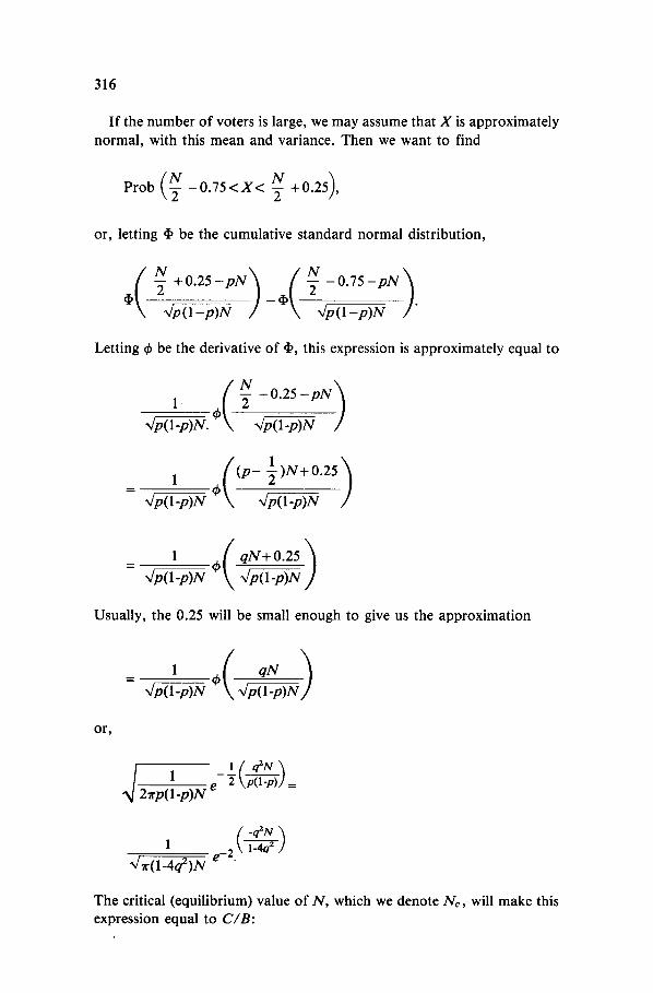
If the number of voters is large, we may assume that X is approximately normal, with this mean and variance. Then we want to find

( ~ ~ ) Prob ~- -0 .75<X< -~ +0.25 ,

or, letting ~I, be the cumulative standard normal distribution,

o(. )~-~N 7- ~ ~ 7

Letting ¢ be the derivative of ~, this expression is approximately equal to

,

~ N - ~ ~ 7

1 ( ( p - ~ ) N + 0.25) - ~ ~ x - ~

I qN+ 0.25 / - - ~ ~ .

Usually, the 0.25 will be small enough to give us the approximation

1

or,

~j _±(CN) _ 1 e 2 \ p ( 1 - p ) , / = 2~rp(1-p)N

, ~_~(~) 4r(1-4qZ)N

The critical (equilibrium) value of N, which we denote No, will make this expression equal to C/B'.

317

( 4q 2 Nc ~ C 2 2 - \ l_4q~/=

e r(1-4q2)Nc B 2 " (6)

This is a transcendental equation, which must be solved for No. While an exact solution is not possible, it is not difficult to solve numerically. In par- ticular we note that the left-hand side decreases as N increases, both because N appears in the denominator and because it appears in the

(negative) exponential. Hence, as the ratio C/B increases, either because B decreases (no great difference between candidates) or because C in- creases (for example, it is difficult to get to the polls), N~ must decrease. Similarly, as q increases (the victor 's lead is seen as large), Nc will decrease. (N~ is independent of A, the number of potential voters.)

A Nash equilibrium exists if the number of people voting is equal to N~, as given by equation (6). There are many alternative equilibria, but we look for a symmetric equilibrium (one in which all citizens choose the same (mixed) strategy) because there is no a priori reason for treating citizens differently. If we asume that other citizens' decisions are fixed, then any given citizens' probabili ty of affecting the election outcome is independent of which candidate he wishes to support. From equation (6) it follows that a symmetric equilibrium obtains if each citizen votes with probabili ty r, such that

r = f ~ / A if N¢<A

if N~ > A

Assuming that N~ _<A, then, the probabili ty that candidate 1 wins is given by

~(. qN~ ~ = ~ ( 2 q N c _ ~ (7)

As an example, suppose that p ~ - , so that q = 0. Then Nc will satisfy

2/TrN~ = C2/B 2 , or N~ = 2B2/~rC 2 .

Thus, in a very close election, the equilibrium number of voters is pro- portional to the square of the difference that the candidates make, and in- versely proportional to the square of the costs of voting. If, for example C/B = 10 -3 , then Nc = 2 x 1 0 6 / 7 1 . = 6.4 x 105 .

But suppose that the election is not so close. I f p = .6, then we will have,

approximately, ~2--~-_ e-.°4:~ = 1 0 - 6 orNce .04No = 6.4 x 103 . ~ l z * c

318

This expression is of the order of Nc = 200. Of course, 60°7o of the votes represents a landslide, and we can understand that, in such an event, there is not much point in voting. But we find that even for p = .51 - hardly a landslide - the critical value of Nc is of the order of 10,000. It is only when the election becomes a cliff-hanger that there is much point to voting: for p = .501, we would have a critical value of approximately 380,000. Even this number is small compared to the American electorate (which is of the order of 10s). We conclude, then, that people must generally be induced

to vote through some argument other than an interest in affecting the elec- tion outcome: no matter how close an election, it is almost inconceivable that one vote will prove decisive, and the slight probability o f this event is simply not great enough to make. the effort (o f voting) worthwhile.

4. Composite voting

Let us now consider the situation that holds under composite voting, for example, in an American presidential election. In this case, there are m constituencies, with A~ ( j = 1,2 . . . . . m) citizens respectively. The citizens f rom the j th constituency elect a delegate with wj 'electoral votes. ' Election is by a majori ty of the electoral votes, arbitrarily defined as q or more, such that usually (but not necessarily),

1 1 )

l J, q ~- q= ~ [ Z w j + or = Z w j + l

(whichever of these is an integer).

In this situation, a citizen who is considering voting for candidate I finds that he will be decisive only if two conditions hold: (a) his vote makes a difference within the constituency (state), and (b) his constituency's elec- toral votes are decisive in the election.

The meaning of (a) is given earlier; the meaning of (b) is best given by saying that s t a t e j is decisive (for 1) if q - w j < ~ wk < q, such that T is the

keT set o f constituencies, other than j , that candidate 1 carries.

The set T is not generally known. Rather, it is a random variable. To simplify matters, we assume that each voter has probabili ty 1/2 of voting for candidate 1; if so, then each constituency also has probabili ty 1/2 of voting for 1, and it follows that Zj = ~ wk is a random variable with

k~T mean/z(Z~) = I / 2 ~ ] w~ and variance o2(Z~) = 1/4~Y~ w, 2 .

k~j k~tj The exact distribution of Zj is very difficult to give. But if we assume

that the number of constituencies is large and that no one constituency is

319

much larger than the others, then we may assume that Z~ is approximately normal. Thus we are looking for the probability, which we denote s~, that q - w ~ - 1/2< Z~ < q - 1/2, with Zj a normal random variable with the given mean and variance. This is approximately

)-+t,- 7' such that • is the normal distribution function. Assuming that q =

1 1 z---x-~w~ + ~ - , this will give us approximately

!8)

sj = 2 ~ I ' / ~ / - 1. (9)

On the other hand, the probability, u~, that a given citizen is decisive in his constituency is

uj = (10)

The probability that the citizen is decisive in the general election is the pro- duct of these two probabilities, sj and uj.

We thus have

s j u j = ,b wj -1 ~r~" (11) Wk

Because the critical number of voters is obtained when this quantity is 2 C 2

= o r equal to C / B , we have ~rN~ B2s~ 2'

2B2 sj 2 N j c - ~rC2 • (12)

Now, equation (12) gives the critical number, N~c, of voters from the j th constituency. In equilibrium, the individual citizens from this constituency should vote with probability rj, such that

320

f N j c / A j if Nj~ -<Aj rj ~ .

if Njc >-A j ,

and such that Aj is the number of eligible citizens in the j th constituency. s~ is the Banzhaf-Coleman index for the weighted majority game (see

Owen, 1975). Under many circumstances, this index is approximately pro- portional to wj. We would then have Njc~kw~ 2, and so, if N j c < A j ,

kw.i 2 rj = Aj " (13)

It seems reasonable that 'a fair' assignment of weights (wj) is one that will hold equal incentives for citizens in each constituency; that is, all r~ should be approximately equal. If so, then the wj should be chosen proportional, not to the district' population, but rather to the square root of the popula- tion. To be somewhat more precise, the weights should be chosen in such a way as to make the Banzhaf-Coleman index, s~, as much as possible pro- portional to the square root of the population (but this choice might in itself be a very complicated problem).

Generally there are three problems with the preceding analysis. First, the assumption that all of the probabilities p~ are equal seems extremely restrictive: in most elections some constituencies have a stronger preference for one candidate than for another. Second, even if all districts have similar preferences (all p~ are equal), it is not clear that the common value

ofp j should be ----~. Third, if we assign weights proportional to the square

root of population, we violate other notions of 'fair' representation (Grof- man and Scarrow, 1981).

Let us consider the second of these objections: we suppose that all p~ are

but different from -~-. We again assume, without loss of equal, generality,

1 that p~ = p = ~ - + q , q>0 . But the quantities xj (the probability that can-

didate 1 carries the constituency) will depend not only on p but also on N~, the number of actual citizens in the region. More exactly, we have the approximation

x)= ~ ~ / (14)

as before; it is clear that, for q>0 , xj will be greatest for those constituen- cies with the largest number of citizens.

321

We can obtain equilibrium values of Nj, depending on the cost-to-

benefit ratio, C/B, and also on p . Since the critical values are all inter- related, however, we will arrive at a very complicated system of equations, the numerical solution of which, while in theory possible, will be quite lengthy.

Qualitatively, it seems likely that the citizens in the smaller constituencies

are advantaged. Indeed, if p is considerably larger than -~-, then uj (given

equation by (10)) decreases quite rapidly as N~ increases, and we can con- clude that, at equilibrium, Njc should increase much less rapidly then A~ (the potential number of citizens). Thus r~ should be relatively smaller for

those constituencies with large populations, although a measurement of the bias seems difficult. If, as is usually the case, w~. is made proport ional to A~, it is difficult to say which values of p will advantage the small, as op- posed to the large constituencies.

There remains the case in which the p~'s differ among constituencies. Ce- teris paribus, the citizens in the 'close' constituencies (those in which p~ is

1 close to -~-) should have the greatest incentive to vote, although exact cal-

culations are quite complex.

5. Conclusions: Vote for the candidate of your choice

Looking back on November 4, 1980 it is apparent that many fewer people voted for John Anderson than had earlier expressed support for him. While we no doubt can explain some of this fallout in the Anderson vote by a disenchantment with the candidate, we can also interpret a very large

part of Anderson 's loss of support as voters being convinced that a vote for Anderson was a 'wasted vote. ' As the compaign continued, it became more and more obvious that Anderson had no real chance to win, or even to get enough electoral votes to put the election into the House of Representatives. Media pundits, the pollsters, and supporters of the major candidates reminded voters who were Anderson supporters that to vote for

Anderson was to throw away any chance they had of affecting the election outcome.

The idea that a third party vote was a 'wasted ' vote, while a vote for Carter or Reagan would not have been wasted, is absurd. It makes sense only if one believes that a citizen, by choosing to cast his vote for Carter or Reagan instead of Anderson (or Clarke or Commoner) , could have had some reasonable expectation that his vote might affect the outcome in favor of one or the other of the major party candidates. But such a belief is nonsensical! Even in an election as close as the Carter-Reagan contest

322

was supposed to have been, no single citizen's vote would have made a discernible difference, even for the electoral outcome in a single state. Moreover, for that citizen's vote to have affected the presidential election, it would not only have had to have determined the outcome in the voter's home state, but also the state's electoral votes would have had to have been critical in providing the winner with the needed victory margin in the Elec- toral College. The product of two such improbabilities is an even greater improbability.

For example, if a citizen had a one-in-3,000 chance of affecting the elec- tion outcome in, say, California (see equation (3)), and if California's elec- toral vote had a one-in-seven chance of providing the winning electoral margin (see exact calculations in Owen, 1975), then a California voter had only a one-in-21,000 chance of affecting the election outcome. 7 Barring improbably high utility for his preferred candidate over his next preferred candidate, if a citizen's only reason for voting was to influence the out- come of the presidential election, he or she would have been best off stay- ing home. s Moreover, one in 3,000 and one in seven are actually wildly op- timistic. One in 3,000 is the probability that a voter in a voting electorate of eight million would cast a decisive vote in a two-candidate contest, in which each voter walking into the ballot booth had exactly a fifty-fifty chance of voting for each candidate and flipped a 'mental ' coin to decide which candidate it would be. Real elections are much more lopsided. In California, where Reagan crushed Carter, the likelihood that a single vote could have affected the outcome was, to put it simply, zero.

An analogous line of reasoning applies for the race within the electoral college. Nationwide, in terms of electoral votes~ the likelihood that a switch of a single state (even a state as large as California) could have affected the outcome was also (see Section 3) roughly zero.

We believe that the implication of such probability calculations is quite clear. I f you are going to bother to vote at all, then never allow yourself to be talked out of voting for the candidate o f your choice. Since your vote is not going to make a difference anyway, you make as well at least have the satisfaction of voting for the candidate whom you prefer.

NOTES

1. The probabilities o f these two outcomes are denoted P3 and p~, for respectively, in Fere- john and Fiorina (1974).

2. For N unknown and sufficiently large, the probability that a given citizen's vote will make a tie is essentially identical to the probability that a given citizen's vote will break a tie.

3. A related but still quite distinctive approach to the citizen's decision calculus is found in Hinich (1981).

4. For N large, N and N-1 are essentially interchangeable. The result is mathematically iden-

323

tical to a well-known theorem in game theory on the properties of the Banzhaf index. (See

Banzhaf, 1965; Lucas, 1976; Owen, 1975.) An alternative approach is to assume that p is

unknown but is distributed according to a distribution F(p), with a cont inuous density ¢f(p) in the neighborhood of 1/2. In this case, Chamberlain and Rothschild (1981) show that the probability of a decisive vote is roughly inverse to N.

5. For p in the range .4 to .6, the first term of the expansion offers a reasonable approxi- mation.

6. Of course, voters have other motivations than electorally instrumental ones (Riker and

Ordeshook, 1968, 1974; Niemi, 1976). Moreover, on most occasions on which citizens go

to the polls, they are entitled to cast ballots in a number of different elections - in some of which the voting electorate may be quite small (Wuffle, 1979).

Also, since the Uni':ed States has more elections (at various levels of government) than

any other country in the world, it is inevitable that there will be some elections that actually

do end in ties. For example, ' the Garfield Heights, Ohio, municipal court judge election

was decided in December 11, 1981, by a flip of a coin after the race was officially declared

a tie - 11,653 votes for each candidate. However, the tie occurred only after 3,000 ballots missing on election night were found, four uncounted ballot cards were discovered ten days

after the election, the board ruled on citizen intent on eleven cards had been incorrectly

punched, and a double count o f a disputed ballot had been corrected' (Election Ad- ministration Reports, January 4, 1982: 5). Moreover, for many citizens much of the burden of 'voting' may be the onus of registering to vote and learning the location o f the polling

place. Once those sunk costs are borne, voting itself may be relatively cheap (Erickson,

1979). We might also note that sometimes if elections are reasonably close (for example,

in the range of 100 votes in the case of a large electorate) courts will order recounts or even

a new election (Finkelstein, 1978: 120-130). However, these qualifications do not

significantly affect our pessimistic conclusions, since what would now be calculated is the

probability t.hat one 's vote would be the one that tips the election close enough so that a

new election or recount would be required; and a similar analysis to that given here would establish this probability to be essentially zero.

One way that incentives to vote might arise for a subset of voters is if they could count on the partisanship o f citizens outside the subset. For example, in a large electorate, if most citizens were committed partisans (and to a significant extent committed citizens), and if

the constituency was reasonably competitive in terms of the distribution of a partisan sup-

port, then independent voters might see an opportunity to be decisive in the small 'effec-

tive' electorate (that is, the electorate consisting of their fellow independent voters whose

votes might swing the election). As the proportion of independents increases, so does the

size of the 'effective' electorate. Thus, the recent breakdown of partisanship in the United

States may have had a double-barrelled impact on turnout , not only reducing voters ' affec- ting ties to the political system but also reducing the perceived efficacy of their votes.

However, in previously noncompetit ive areas, the 'Solid South ' for example, the reduction in turnout at tending decreased partisan loyalties might be compensated for by an increase

in turnout created by increased overall electoral competitiveness.

If we consider the most realistic three-candidate case - one in which there are two major candidates, 1 and 2, and one minor candidate, 3, in which only one o f the major candidates can win a clear plurality and the minor candidate could at best achieve a three-way tie - it is easy to show that the addition of a third (minor) candidate increases the likelihood that

1 a given voter 's ballot will affect the election outcome by a factor of only , that is, by

a factor o f only roughly 1.22 (see McKelvey and Ordeshook, 1972; Aranson, 1971). 7. An analogous argument applies to citizens of smaller states. Their chances of deciding their

324

home state's electoral votes will be higher, since the electorate is smaller; but since their state has fewer electoral votes, the likelihood that its vote will provide a decisive electoral margin for the winner is correspondingly reduced. The figure of one seventh, would go down, for example, to one-in-one hundred for the state of South Carolina. See Owen 0975) and Section 3.

8. Cf. Frerejohn and Fiorina (1974, 1975).

REFERENCES

Aranson, P.H. (1971). Politicalparticipation in alternative election systems. Presented at the Annual Meeting of the American Political Science Association, Chicago, September 7-11, 1971.

Banzhaf, J. III. (1965). Weighted voting doesn't work: A mathematical analysis. Rutgers Law Review 19: 317-343.

Beck, N. (1975). A note on the probability of a tied election. Public Choice 23(Fall): 75-80. Chamberlain, G., and Rothschild, M. (1981). A note on the probability of casting a decisive

vote. Journal o f Economic Theory 25 (August): 152-162. Coleman, J. (1971). Control of collectivities and the power of a collectivity to act. In B.

Lieberman (Ed.), Social choice. New York: Simon and Schuster. Downs, (1957). An economic theory o f democracy. New York: Harper and Row. Erickson, R. (1979). Why do people vote? Because they are registered. Presented at the Con-

ference on Voter Turnout, San Diego, May 16-19. Feller, W. (1957). An introduction to probability theory and its application, I. New York:

Wiley. Ferejohn, J., and Fiorina, M. (1974). The paradox of not voting: A decision theoretic

analysis. American Political Science Review 68(June): 525-536. Ferejohn, J., and Fiorina, M. (1975). Closeness counts only in horseshoes and dancing.

American Political Science Review 49(Sept.): 920-925. Finkelstein, M.O. (1978). Quantitative methods in law. New York: Free Press. Good, I.J., and Mayer, L.S. (1975). Estimating the efficacy of a vote. Behavioral Science

20:25-33. Grofman, B. (1981). Fair apportionment and the Banzhaf Index. American Mathematics

Monthly 88(- ): 1-5. Grofman, B., and Scarrow, H. (1981). Riddle of apportionment: Equality of what? National

Civic Review 70, 5(May): 242-254. Hinich, M.J. (1981). Voting as an act of contribution. Public Choice 36: 135-140. Linehan, W.J., and Schrodt, P.A. (1979). Size, competitiveness and the probability o f in-

fluencing an election. Presented at the Conference on Voter Turnout, San Diego, May 16-19.

Lucas, W.F. (1974). Measuring power in weighted voting systems. Case Studies in Applied Mathematics. Mathematics Association of America, Module in Applied Mathematics, 1976. (Originally published as Technical Report No. 227, Department of Operations Research, College of Engineering, Cornell University, Ithaca, N.Y, September.)

Margolis, H. (1977). Probability of a tied election. Public Choice 31(Fall): 135-138. McKelvey, R.D., and Ordeshook, P.C. (1972). A general theory of the calculus of voting. In

J.F. Herndon and J.L. Bernd (Eds.), Mathematical applications in political science, Vol. 6, Charlottesville, Va.: University press of Virginia.

Meehl, P.E. (1977). The selfish citizen paradox and the throw away vote argument. American Political Science Review 71(March): 11-30.

325

Niemi, R.G. (1976). Costs of voting and nonvoting. Public Choice 27(Fall): 115-119. Owen, G. (1979). Multilinear extensions and the Banzhaf value. Naval Research Logistics

Quarterly 22, 4(Dec.): 741-750. Riker, W.H., and Ordeshook, P.C. (1974). A n introduction to positive political theory.

Englewood Cliffs, N.J.:Prentice-Hall. Riker, W.H., and Ordeshook, P.C. (1968). A theory of the calculus of voting. American

Political Science Review62 (March): 25-43. Wuffle, A. (1979). Should you brush your teeth on November 4, 1980? Paper not prepared

for delivery at the Conference on Voter Turnout, San Diego, May 16-19, 1979.