to the theory of galaxies rotation and the hubble

Journal of Modern Physics, 2012, 3, 1103-1122 http://dx.doi.org/10.4236/jmp.2012.329145 Published Online September 2012 (http://www.SciRP.org/journal/jmp)

To the Theory of Galaxies Rotation and the Hubble Expansion in the Frame of Non-Local Physics

Boris V. Alexeev Moscow Lomonosov State University of Fine Chemical Technologies, Prospekt Vernadskogo, Moscow, Russia

Email: [email protected]

Received May 4, 2012; revised June 9, 2012; accepted June 17, 2012

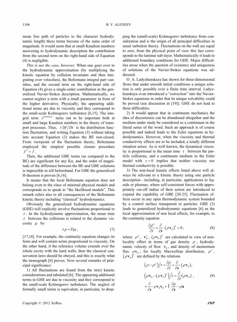
ABSTRACT

The unified generalized non-local theory is applied for mathematical modeling of cosmic objects. For the case of galaxies the theory leads to the flat rotation curves known from observations. The transformation of Kepler’s regime into the flat rotation curves for different solitons is shown. The Hubble expansion with acceleration is explained as result of mathematical modeling based on the principles of non-local physics. Peculiar features of the rotational speeds of galaxies and effects of the Hubble expansion need not in the introduction of new essence like dark matter and dark energy. The origin of difficulties consists in the total Oversimplification following from the principles of local physics. Keywords: Dark Matter; Dark Energy; Galaxy: Halo; Galaxy: Kinematics and Dynamics; Hubble Expansion;

Hydrodynamics

1. Introduction

More than ten years ago, the accelerated cosmological expansion was discovered in direct astronomical observations at distances of a few billion light years, almost at the edge of the observable Universe. This acceleration should be explained because mutual attraction of cosmic bodies is only capable of decelerating their scattering. It means that we reach the revolutionary situation not only in physics but also in the natural philosophy on the whole. Practically we are in front of the new challenge since Newton’s Mathematical Principles of Natural Philosophy was published. As result, new idea was introduced in physics about existing of a force with the opposite sign, which is called universal antigravitation. Its physical source is called as dark energy that manifests itself only because of postulated property of providing antigravitation.

It was postulated that the source of antigravitation is “dark matter” which inferred to exist from gravitational effects on visible matter. However, from the other side dark matter is undetectable by emitted or scattered elec- tromagnetic radiation. It means that new essences—dark matter, dark energy—were introduced in physics only with the aim to account for discrepancies between measurements of the mass of galaxies, clusters of galaxies and the entire universe made through dynamical and general relativistic means, measurements based on the mass of the visible “luminous” matter. It could be reasonable if we are speaking about small corrections to the system of know-

ledge achieved by mankind to the time we are living. But mentioned above discrepancies lead to affirmation, that dark matter constitutes 80% of the matter in the Universe, while ordinary matter makes up only 20%.

Dark matter was postulated by Swiss astrophysicist Fritz Zwicky of the California Institute of Technology in 1933. He applied the virial theorem to the Coma cluster of galaxies and obtained evidence of unseen mass. Zwicky estimated the cluster’s total mass based on the motions of galaxies near its edge and compared that estimate to one based on the number of galaxies and total brightness of the cluster. He found that there was about 400 times more estimated mass than was visually observable. The gravity of the visible galaxies in the cluster would be far too small for such fast orbits, so something extra was required. This is known as the “missing mass problem”. Based on these conclusions, Zwicky inferred that there must be some non-visible form of matter, which would provide enough of the mass, and gravity to hold the cluster together.

The work by Vera Rubin (see for example [1,2]) re- vealed distant galaxies rotating so fast that they should fly apart. Outer stars rotated at essentially the same rate as inner ones (~254 km/s). This is in marked contrast to the solar system where planets orbit the sun with velocities that decrease as their distance from the centre increases. By the early 1970s, flat rotation curves were routinely detected. It was not until the late 1970s, however, that the community was convinced of the need for dark matter halos around spiral galaxies. The mathematical modeling

Copyright © 2012 SciRes. JMP

B. V. ALEXEEV 1104

(based on Newtonian mechanics and local physics) of the rotation curves of spiral galaxies was realized for the various visible components of a galaxy (the bulge, thin disk, and thick disk). These models were unable to predict the flatness of the observed rotation curve beyond the stellar disk. The inescapable conclusion, assuming that Newton’s law of gravity (and the local physics description) holds on cosmological scales, that the visible galaxy was embedded in a much larger dark matter (DM) halo, which contributes roughly 50% - 90% of the total mass of a galaxy. As result another models of gravitation were in- volved in consideration—from “improved” Newtonian laws (such as modified Newtonian dynamics and tensor- vector-scalar gravity [3]) to the Einstein’s theory based on the cosmological constant [4]. Einstein introduced this term as a mechanism to obtain a stable solution of the gravitational field equation that would lead to a static Universe, effectively using dark energy to balance gravity.

Computer simulations with taking into account the hypothetical DM in the local hydrodynamic description include usual moment equations plus Poisson equation with different approximations for the density of DM

DM containing several free parameters. Computer simulations of cold dark matter (CDM) predict that CDM particles ought to coalesce to peak densities in galactic cores. However, the observational evidence of star dynamics at inner galactic radii of many galaxies, including our own Milky Way, indicates that these galactic cores are entirely devoid of CDM. No valid mechanism has been demonstrated to account for how galactic cores are swept clean of CDM. This is known as the “cuspy halo problem”. As result, the restricted area of CDM influence introduced in the theory. As we see the concept of DM leads to many additional problems.

I do not intend to review the different speculations based on the principles of local physics. I see another problem. It is the problem of Oversimplification—but not “trivial” simplification of the important problem. The situation is more serious—total Oversimplification based on principles of local physics, and obvious crisis, we see in astrophysics, simply reflects the general shortcomings of the local kinetic transport theory. It is important to underline that we should have expected this crisis of local statistical physics after the discovery of Bell’s fundamental inequalities [5]. The antigravitation problem in application to the theory of galaxies rotation and the Hubble expansion is solved further in the frame of non-local statistical physics and the Newtonian law of gravitation.

I deliver here some main ideas and deductions of the generalized Boltzmann physical kinetics and non-local physics. For simplicity, the fundamental methodic aspects are considered from the qualitative standpoint of view avoiding excessively cumbersome formulas. A rigorous

description can be found, for example, in the monograph [6].

In 1872 L. Boltzmann [7,8] published his kinetic equation for the one-particle distribution function (DF) , , tr v . He expressed the equation in the form f

BDf Dt J f , (1) BJ is the local collision integral, and where

D

Dt t

v Fr v

v

n T

0BJ 0

is the substantial (particle) de-

rivative, and r being the velocity and radius vector of the particle, respectively. Boltzmann Equation (1) governs the transport processes in a one-component gas, which is sufficiently rarefied that only binary collisions between particles are of importance and valid only for two character scales, connected with the hydrodynamic time-scale and the time-scale between particle collisions. While we are not concerned here with the explicit form of the collision integral, note that it should satisfy con- servation laws of point-like particles in binary collisions. Integrals of the distribution function (i.e. its moments) determine the macroscopic hydrodynamic characteristics of the system, in particular the number density of particles and the temperature . The Boltzmann equation (BE) is not of course as simple as its symbolic form above might suggest, and it is in only a few special cases that it is amenable to a solution. One example is that of a maxwellian distribution in a locally, thermodynamically equilibrium gas in the event when no external forces are present. In this case the equality and f f is met, giving the maxwellian distribution function 0f . A weak point of the classical Boltzmann kinetic theory is the way it treats the dynamic properties of interacting particles. On the one hand, as the so-called “physical” derivation of the BE suggests, Boltzmann particles are treated as material points; on the other hand, the collision integral in the BE brings into existence the cross sections for collisions between particles. A rigorous approach to the derivation of the kinetic equation for f (noted in following as fKE ) is based on the hierarchy of the Bogolyubov- Born-Green-Kirkwood-Yvon (BBGKY) [6,9-13] equations.

A fKE obtained by the multi-scale method turns into the BE if one ignores the change of the distribution function (DF) over a time of the order of the collision time (or, equivalently, over a length of the order of the particle interaction radius). It is important to note [6,14] that ac- counting for the third of the scales mentioned above leads (prior to introducing any approximation destined to break the Bogolyubov chain) to additional terms, generally of the same order of magnitude, appear in the BE. If the correlation functions is used to derive fKE from the BBGKY equations, then the passage to the BE means the neglect of non-local effects.


B. V. ALEXEEV 1105

Given the above difficulties of the Boltzmann kinetic theory, the following clearly inter related questions arise. First, what is a physically infinitesimal volume and how does its introduction (and, as the consequence, the un- avoidable smoothing out of the DF) affect the kinetic equation? This question can be formulated in (from the first glance) the paradox form—what is the size of the point in the physical system? Second, how does a sys- tematic account for the proper diameter of the particle in the derivation of the fKE affect the Boltzmann equation? In the theory developed here, I shall refer to the corresponding fKE

r vt

as Generalized Boltzmann Equa- tion (GBE). The derivation of the GBE and the applications of GBE are presented, in particular, in [6]. Accord- ingly, our purpose is first to explain the essence of the physical generalization of the BE.

Let a particle of finite radius be characterized, as before, by the position vector and velocity of its center of mass at some instant of time . Let us introduce physically small volume (PhSV) as element of measurement of macroscopic characteristics of physical system for a point containing in this PhSV. We should hope that PhSV contains sufficient particles ph for statistical description of the system. In other words, a net of physically small volumes covers the whole investi- gated physical system.

N

Every PhSV contains entire quantity of point-like Boltzmann particles, and the same DF f is prescribed for whole PhSV in Boltzmann physical kinetics. There- fore, Boltzmann particles are fully “packed” in the reference volume. Let us consider two adjoining physically small volumes 1 and 2PhSV . We have in principle another situation for the particles of finite size moving in physical small volumes, which are open thermodynamic systems.

PhSV

Then, the situation is possible where, at some instant of time t, the particle is located on the interface between two volumes. In so doing, the lead effect is possible (say, for 2 ), when the center of mass of particle moving to the neighboring volume 2 is still in 1 . However, the delay effect takes place as well, when the center of mass of particle moving to the neighboring volume (say, 2 ) is already located in but a part of the particle still belongs to .

PhSVPhSV PhSV

2PhSVPhSV

1

Moreover, even the point-like particles (starting after the last collision near the boundary between two mentioned volumes) can change the distribution functions in the neighboring volume. The adjusting of the particles dynamic characteristics for translational degrees of free- dom takes several collisions. As result, we have in the definite sense “the Knudsen layer” between these volumes. This fact unavoidably leads to fluctuations in mass and hence in other hydrodynamic quantities. Existence of such “Knudsen layers” is not connected with the choice

of space nets and fully defined by the reduced description for ensemble of particles of finite diameters in the con- ceptual frame of open physically small volumes, therefore—with the chosen method of measurement.

PhSV

This entire complex of effects defines non-local effects in space and time. The corresponding situation is typical for the theoretical physics—we could remind about the role of probe charge in electrostatics or probe circuit in the physics of magnetic effects.

f corresponds to 1 and DF PhSVSuppose that DF f f PhSV is connected with 2 for Boltzmann parti-

cles. In the boundary area in the first approximation, fluctuations will be proportional to the mean free path (or, equivalently, to the mean time between the collisions). Then for PhSV the correction for DF should be introduced as

af f Df Dt (2)

in the left hand side of classical BE describing the trans- lation of DF in phase space. As the result

a BDf Dt J , (3) BJ is the Boltzmann local collision integral. where

Important to notice that it is only qualitative explana- tion of GBE derivation obtained earlier (see for example [6]) by different strict methods from the BBGKY—chain of kinetic equations. The structure of the K fE is generally as follows

B nonlocalDfJ J

Dt

nonlocalJ

, (4)

where is the non-local integral term incorpo- rating the non-local time and space effects. The generalized Boltzmann physical kinetics, in essence, involves a local approximation

nonlocal D DfJ

Dt Dt

(5)

for the second collision integral, here in the simplest case being the mean time between the particle collisions. We can draw here an analogy with the Bhatnagar- Gross-Krook (BGK) approximation for BJ ,

0B f fJ

, (6)

which popularity as a means to represent the Boltzmann collision integral is due to the huge simplifications it of- fers. In other words—the local Boltzmann collision integral admits approximation via the BGK algebraic expression, but more complicated non-local integral can be expressed as differential form (5). The ratio of the second to the first term on the right-hand side of Equation (4) is given to an order of magnitude as and at large Knudsen numbers (Kn defining as ratio of

2Knnonlocal BJ J O


B. V. ALEXEEV 1106

mean free path of particles to the character hydrodynamic length) these terms become of the same order of magnitude. It would seem that at small Knudsen numbers answering to hydrodynamic description the contribution from the second term on the right-hand side of Equation (4) is negligible.

This is not the case, however. When one goes over to the hydrodynamic approximation (by multiplying the kinetic equation by collision invariants and then inte- grating over velocities), the Boltzmann integral part van- ishes, and the second term on the right-hand side of Equation (4) gives a single-order contribution in the generalized Navier-Stokes description. Mathematically, we cannot neglect a term with a small parameter in front of the higher derivative. Physically, the appearing additional terms are due to viscosity and they correspond to the small-scale Kolmogorov turbulence [6,15]. The integral term turns out to be important both at small and large Knudsen numbers in the theory of transport processes. Thus,

nonlocalJ

Df Dt is the distribution function fluctuation, and writing Equation (3) without taking into account Equation (2) makes the BE non-closed. From viewpoint of the fluctuation theory, Boltzmann employed the simplest possible closure procedure

af f . Then, the additional GBE terms (as compared to the

BE) are significant for any Kn, and the order of magnitude of the difference between the BE and GBE solutions is impossible to tell beforehand. For GBE the generalized H-theorem is proven [6,16].

It means that the local Boltzmann equation does not belong even to the class of minimal physical models and corresponds so to speak to “the likelihood models”. This remark refers also to all consequences of the Boltzmann kinetic theory including “classical” hydrodynamics.

Obviously the generalized hydrodynamic equations (GHE) will explicitly involve fluctuations proportional to . In the hydrodynamic approximation, the mean time between the collisions is related to the dynamic viscosity by

p , (7)

[17,18]. For example, the continuity equation changes its form and will contain terms proportional to viscosity. On the other hand, if the reference volume extends over the whole cavity with the hard walls, then the classical con-servation laws should be obeyed, and this is exactly what the monograph [6] proves. Now several remarks of prin-cipal significance:

1) All fluctuations are found from the strict kinetic considerations and tabulated [6]. The appearing additional terms in GHE are due to viscosity and they correspond to the small-scale Kolmogorov turbulence. The neglect of formally small terms is equivalent, in particular, to drop-

ping the (small-scale) Kolmogorov turbulence from consideration and is the origin of all principal difficulties in usual turbulent theory. Fluctuations on the wall are equal to zero, from the physical point of view this fact corresponds to the laminar sub-layer. Mathematically it leads to additional boundary conditions for GHE. Major difficulties arose when the question of existence and uniqueness of solutions of the Navier-Stokes equations was ad- dressed.

O. A. Ladyzhenskaya has shown for three-dimensional flows that under smooth initial conditions a unique solution is only possible over a finite time interval. Ladyz- henskaya even introduced a “correction” into the Navier- Stokes equations in order that its unique solvability could be proved (see discussion in [19]). GHE do not lead to these difficulties.

2) It would appear that in continuum mechanics the idea of discreteness can be abandoned altogether and the medium under study be considered as a continuum in the literal sense of the word. Such an approach is of course possible and indeed leads to the Euler equations in hydrodynamics. However, when the viscosity and thermal conductivity effects are to be included, a totally different situation arises. As is well known, the dynamical viscosity is proportional to the mean time between the particle collisions, and a continuum medium in the Euler model with 0 implies that neither viscosity nor thermal conductivity is possible.

3) The non-local kinetic effects listed above will al- ways be relevant to a kinetic theory using one particle description—including, in particular, applications to liquids or plasmas, where self-consistent forces with appro- priately cut-off radius of their action are introduced to expand the capability of GBE [20-25]. Fluctuation effects occur in any open thermodynamic system bounded by a control surface transparent to particles. GBE (3) leads to generalized hydrodynamic equations [6] as the local approximation of non local effects, for example, to the continuity equation

0 0a

a

t

v

ra

, (8)

where , 0 , 0 are calculated in view of non- locality effect in terms of gas density

av av , hydrody-

namic velocity of flow 0 , and density of momentum flux 0

vv a; for locally Maxwellian distribution, ,

are defined by the relations 0

av

0

0 0 0

0 0

,

I

a

a

t

tp

vr

v v v

v v аr r

, (9)


B. V. ALEXEEV 1107

where is a unit tensor, and is the acceleration due to the effect of mass forces.

I

a

In the general case, the parameter is the non-locality parameter; in quantum hydrodynamics, the “time- energy” uncertainty relation defines its magnitude. The violation of Bell’s inequalities [5] is found for local statistical theories, and the transition to non-local description is inevitable. The following conclusion of principal significance can be done from the generalized quantum consideration [22,23]:

1) Madelung’s quantum hydrodynamics is equivalent to the Schrödinger equation (SE) and leads to description of the quantum particle evolution in the form of Euler equation and continuity equation.

2) SE is consequence of the Liouville equation as re-sult of the local approximation of non-local equations.

3) Generalized Boltzmann physical kinetics defines the strict approximation of non-local effects in space and time and after transmission to the local approximation leads to parameter , which on the quantum level corresponds to the uncertainty principle “time-energy”.

4) GHE lead to SE as a deep particular case of the generalized Boltzmann physical kinetics and therefore of non-local hydrodynamics.

In principal GHE needn’t in using of the “time-energy” uncertainty relation for estimation of the value of the non-locality parameter . Moreover, the “time-energy” uncertainty relation does not lead to the exact relations and from position of non-local physics is only the simplest estimation of the non-local effects.

Really, let us consider two neighboring physically in- finitely small volumes 1 and 2 in a non- equilibrium system. Obviously the time

PhSV PhSV should tend

to diminish with increasing of the velocities of particles invading in the nearest neighboring physically infi- nitely small volume ( or ):

u

2PhSV1hSVPnH u . (10)

However, the value cannot depend on the velocity direction and naturally to tie with the particle kinetic energy, then

2 ,H mu (11)

where H is a coefficient of proportionality, which reflects the state of physical system. In the simplest case H is equal to Plank constant and relation (11) becomes compatible with the Heisenberg relation.

non-local effects can be discussed from viewpoint of

adjoin

ons I i nified ge

e dark matter is not signifi- ca

tion curves have the character fla

possible to obtain the continuous transition fr

he explo- si

her words—is it possible using only Newtonian gr

2. Disk Galaxy Rotation and the Problem of

Ab after Zwicky’s initial observations

of the type B corresp

Finally, we can state that introduction of open control volume by the reduced description for ensemble of particles of finite diameters leads to fluctuations (proportional to Knudsen number) of velocity moments in the volume. This fact defines the significant reconstruction of the theory of transport processes. Obviously the mentioned

breaking of the Bell’s inequalities [5] because in the non-local theory the measurement (realized in 1PhSV ) has influence on the measurement realized in the - ing space-time point in 2PhSV and verse versa.

In the following secti ntend to apply the uneralized non-local theory for mathematical modeling

of cosmic objects. For the case of galaxies the theory leads to the flat rotation curves known from observations. The transformation of Kepler’s regime into the flat rotation curves for different solitons is shown. The Hubble expansion with acceleration is explained as result of mathematical modeling based on the principals of non- local physics. Therefore the answers for the following questions are formulated:

1) Why the concept of thnt in the Solar system? 2) Why the galaxy rotat form? 3) Is it

om the Kepler regime to the flat halo curves? 4) Why after Big Bang explosion (or after t

on in the Hubble boxes) the Hubble expansion exists with acceleration? ([26-28], Nobel Prize for the observ- ers S. Perlmutter, A. G. Riess, B. Schmidt of the year 2011).

In otavitation law and non-local statistical description to

forecast the flat gravitational curve of a typical spiral galaxy (Section 2) and the Hubble expansion (including the Hubble expansion with acceleration, PRS-regime), (Section 3)? The last question has the positive answer.

Dark Matter

out forty years Vera Rubin, astronomer at the Department of Terrestrial Magnetism at the Carnegie Institution of Washington presented findings based on a new sensitive spectrograph that could measure the velocity curve of edge-on spiral galaxies to a greater degree of accuracy than had ever before been achieved. Together with Kent Ford, Rubin announced at a 1975 meeting of the American Astro- nomical Society the astonishing discovery that most stars in spiral galaxies orbit at roughly the same speed reflected schematically on Figure 1.

For example, the rotation curve onds to the galaxy NGC3198. The following extensive

radio observations determined the detailed rotation curve of spiral disk galaxies to be flat (as the curve B), much beyond as seen in the optical band. Obviously the trivial balance between the gravitational and centrifugal forces leads to relation between orbital speed V and galacto- centric distance r as 2

NV M r bey nd the physical extent of the galaxy of m

oass M (the curve A). The


B. V. ALEXEEV

JMP

1108

obvious contradiction with the velocity curve B having a “flat” appearance out to a large radius, was explained by introduction of a new physical essence—dark matter because for spherically symmetric case the hypothetical density distribution

Vel

ocit

y

B

2~ 1r r V const leads to . The result of this activity is known—undetectable dark matter which does not emit radiation, inferred solely from its gravitational effects. But it means that upwards of 50% of the mass of galaxies was contained in the dark galactic halo.

A

Strict consideration leads to the following system of the generalized hydrodynamic equations (GHE) [6,22-25, 29-31] written in the generalized Euler form:

Distance

Figure 1. Rotation curve of a typical spiral galaxy: pre- ) (Continuity equation for species dicted (A) and observed (B).

Copyright © 2012 SciRes.

0

10 0 0I .

t t

p qR

t m

0 0

vr

v v v v F v Br r r

(12)

(Continuity equation for mixture)

0

(1)0 0 0 0 0I 0

t t

p q

t m

vr

v v v v F v Br r r

(13)

.

(Momentum equation for species )

10 0 0 0 0

10

10

p q

t t m

t

q p q

v v v v F v Br r

F vr

v B B0 0 0 0

0 0 0I

m t m

pt

v v v v Fr r

v v vr

(1) (1)0 0 0 0 0 0 0

I

2I

I

p

p

q qp

m m

0

0 0 0 0

, ,d d .st el st inelm J m J

v

v v v vr r

v F v v F v B v v v Br

(14)

v v v v

(Momentum equation for mixture)

B. V. ALEXEEV 1109

(1) (1)0 0 0 0 0

(1)0 0 0 0 0

0 0 I

p q

t t m

q p q

m t m

p

0t

v v v v F v B F vr r r

v v v v F v B Br r

v vr

0 0 0 0 0 0

(1) (1)0 0 0 0 0 0 0

I 2I

I 0

p pt

q qp

m m

v v v v v vr r

v F v v F v B v v v Br

(15)

(Energ ation for y equ species)

20 03v 2

2 (1)0 0 0 0 0

2 20 0 0 0 0 0 0 0

20 0 0 0

3 1 5

2 2 2 2 2 2

1 5 1 5

2 2 2 2

1 7

2 2

vp n p n v p n

t t

v p n v p nt

v p

v v v F vr

v v v v v vr

v v v vr

22

0 0 0 0

2(1) (1) 2 (1) (1) 0

0 0 0 0

(1)0 0

(1) (1)0 0 0 0

1 5

2 2

1 3

2 2 2

5

2

p pp v n

m

v qp v p

m

q qp n n

m m

pt

v v

F v v F F F v B

v B v B F

F v F v v vr r

(1)

0

2 2, ,d d .

2 2st el st inel

q n

m v m vJ J

F v B

v v

(16)

(Energy equation for mixture)

202

00 0 0 0

2 20 0 0 0 0 0 0 0

20 0 0

33 1

2 22 2 2 2

1 5 1 5

2 2 2 2

1 7

2 2

vp nv

p n v p ntt

v p n v p nt

v

2 (1)0

5

v v v F vr

v v v v v vr

v vr

22

0 0 0 0 0

2(1) (1) 2 (1) (1) 0

0 0 0 0 0

(1)0

(1) (1)0 0 0 0

1 5

2 2

1 3 5

2 2 2 2

p pp p v n

m

v q qp v p p

m m

qn n

m

t

v v v v

F v v F F F v B v B

v B F

v F F v v vr

(1)0 0.p q n

F v B

r

(17)


B. V. ALEXEEV


1110

Here 1

F are the forces of the non-magnetic origin, B —magnet nduction, I

t tensor, qic i —uni —charge

of the α-com particleponent , p —static pressure for poneα-com nt, —in

0 — hyternal en y for the particles of

pone v drody c velocity for mixture, erg

namiα-com nt,

—non ter. GHE can ap lied to the ysical systems from the

Universe to atomic scales. All additional explanations will be done by delivering the results of modeling of corresponding physical systems with the special consideration of non-lo arameters

-local pa be

ramep ph

cal p . Generally speaking to GHE should dded the system of generalized Maxwell equations (for example in the form of the generalized Poisson equation for electric potential) and gravitational equations (for example in the form of the generalized Poisson equation for gravitational potential).

In the following I intend to show that the character features reflected on Figure 1 can be explained in the framki

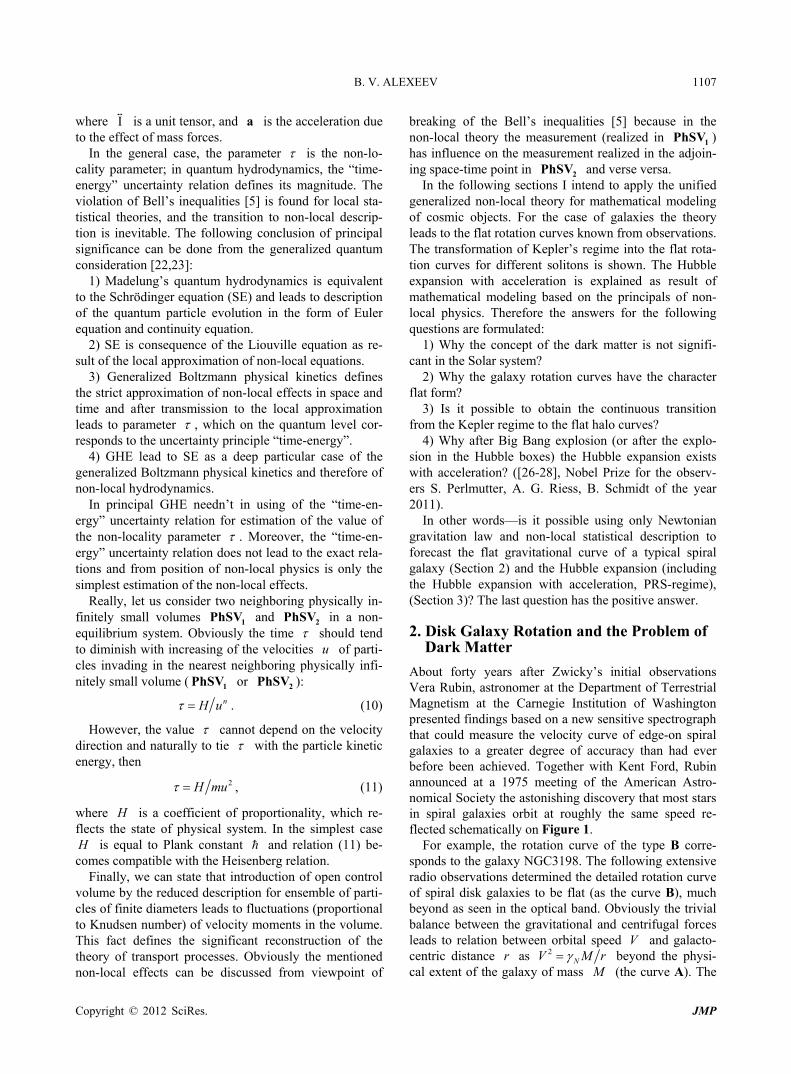
consider the formation of the soliton’s type of solution of the generalized hydrodynamic equations for gravitational media like galaxy in the self consistent gravitational field. Our aim consists in calculation of the self-consistent hydrodynamic moments of possible formation like gravitational soliton.

Let us investigate of the gravitational soliton formation in the frame of the non-stationary 1D Cartesian formula- tion. Then the system of GHE consist from the gized Poisson equation reflecting the effects of the density and the density flux perturbations, continuity equation, motion and energy equations. The GHE derivation can be found in [6,15,29]. This system of four equations for non-stationary 1D case is written as the deep particular case of Equations (12)-(17) in the form:

(Poisson equation)

be a

eneral-

e of Newtonian gravitation law and the non-local netic description created by me. With this aim let us

2

24π N u

t xx

, (18)

(Continuity equation)

2 0,p

ux x x

(19) u u

t t x x t

u

(Motion equation)

2

2 2 3 3 u

2 0,

ux t x

ux

p

u u ut t x x x

u p u p u px t x

(20)

(Energy equation)

2 23 3u p u pt t x

3

3 3

2 2

5 2

5 5 8 5

3 5 2 0,

u pu ux

u pu u pu u p ux t x

u p u u u px x t x x

(21)

(

24 2 p

where u is translational velocity of the one species object, —self consistent gravitational potential

Taking into accowait that the group v

unt the De Broglie relation we should elocity gu is equal 2 0u . In moving

coordinate system all dependent hydrodynamic values are function of

g r is acceleration in gravitational field), is density and p is pressure, , t is non-locality pa- . W

n of the soliton type. For this solution xplicit dependence on time for coordinate g with the phase velocity 0u . Write down

of Equations (18)-(21) in the dimensionless imensionless symbols are marked by tildes.

e investigate the possibility of the object formatiothere is no esystem movinthe systemform, where d

rameter, N is Newtonian gravitation constant. Let us introduce the coordinate system moving along

the positive direction of x-axis in ID space with velocity C u equal to phase velocity of considering object 0

x Ct . (22)

B. V. ALEXEEV 1111

For the scales 0 0 0, ,u x 20 0 0 0,u t u , 2 2

0 0 0 0u xN ,

0 0 0p u2 and conditions 0 1C C u , the equations take the form

(Generalized Poisson equation)

:

2

24π N u

, (23)


2 2 0,p u u

(24)

u

(Mot quation) ion e

2 u

u

22u p u u 32 3p u pu

2u 0,

(25

(Energy equation)

)

23 4 2

2

1 8 5

2

pu pu

u

u u p

2 3

2

3 5 2

3 5 2 2

u p u pu u

u p u

20 3pu u p

0,

(26)

the system of four ordinary non- linear Equations (23)-(26):

1) Every equation from the system is of the second order and needs two conditions. The problem belongs to the class of Cauchy problems.

2) In comparison for example, with the Schrödinger theory connected with behavior of the wave function, no special conditions are applied for dependent variables in of the solution existing. This domain is defined automatically in the process of the numerical solution of the concrete variant of calculations.

3) From the introduced scales 20 0 0 0 0 0 0, , ,u x u t u ,

Some comments to

cluding the domain

2 20 0 0 0N u x , 2

0 0 0p u , only three parameters are independent, namely, 0 0 0, ,u x .

4) Approximation for the dimensionless non-local parameter should be introduced (see (11)). In the definite sense it is not ynamic level

e calculation of drodynamics).

the problem of the hydrodm description (like thts in the classical hy

of the the Int

physical systekinetic coefficien

eresting to notice that quantum GHE were applied with success for calculation of atom structure [22-25], which is considered as two species charged ,e i mixture. The corresponding approximations for non-local parameters i , e and ei are proposed in [22,23]. In the theory of the atom structure [23] after taking into

account the Balmer’s relation, (11) transforms into

2e en m u , (27)

where 1, 2,n is principal quasult the length scale relation was written as

ntum number. As re-

0 0 0e eH m u n m u . But the value x quev m

has the dimension 2cm s and can be titled as quantum viscosity, 21.1577cm s.quv Then

2que nv u . (28)

Introduce now the quantum Reynolds number

0 0Requ quu x v . (29)

As result from (27)-(29) follows the condition quantization for Requ . Namely

Re , 1, 2,qu n n (30)

5) Taking into account the previous considerations I in

of

troduce the following approximation for the dimensionless non-local parameter

21 u , (31)

2 2ku x u u , (32) 0 0 0


B. V. ALEXEEV 1112

where the scale for the kinematical viscosity is intro-

0 0 the physically transparent result—non-l

d in i proportion to the sq

duced 0k u x . Then we have -

ocal parameter is proportional to the kinematical viscosity an nverse

uare of velocity. The system of generalized hydrodynamic Equations

(23)-(26) (solved with the help of Maple) have the great possibilities of mathematical modeling as result of changing of eight Cauchy conditions describing the character features of initial perturbations which lead to the soliton formation. The following Maple notations on figures are used: r—density , u—veloc u , p— pressure p and v—self consistent potential .

Explanations placed under all following figures, Maple program contains Maple’s notations—for example the expression 0 0D u means in the usual nota

ity

tions u 0 0 , indepe ndent variable t responds to .

gin with

Cauchy condition avitationaobject of the soliton’s kind

ith thins ( I 1 ,

We be investigation of the problem of principle significance—is it possible after a perturbation (defined by

Figure. 3. p pressure p (dashed line), u velocity u in gravitational soliton.

s) to obtain the gr l as result of the self-organiza-

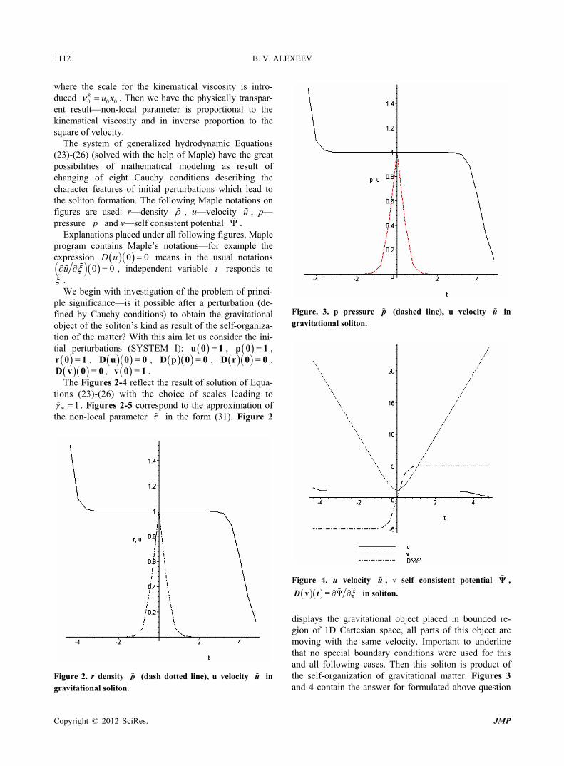
tion of the matter? W s aim let us consider the initial perturbatio u 0 = SYSTEM ): p 0 = 1 , r 0 = 1 , D u 0 = 0 , p 0 = 0 , D r 0 = 0 , D D v 0 = 0 , v 0 = 1 . The Figures 2-4 reflect the result of solution of Equa-

tions (23)-(26) with the choice of scales leading t1N

o . Figures 2-5 correspond toth

the approximation of e non-local parameter in the form (31). Figure 2

Figure 4. u velocity u , v self consistent potential Ψ ,

v Ψ D t = ξ in soliton.

displays the gravitational object placed in bounded region of 1D Cartesian space, all parts of this object are moving with the same velocity. Important to underline that no special boundary conditions were used for this and all following cases. Then this soliton is product of the self-organization of gravitational matter. Figures 3 and 4 contain the answer for formulated above question

Figure 2. r density ρ (dash dotted line), u velocit u in gravitational soliton.

y


B. V. ALEXEEV 1113

Figure 5. u velocity u , density r ρ , v ΨD t = ξ in

soliton, ( γ = 0.01 ). N

about stability of the object. The derivative (see Figure 4)

0 0x g2020

xg u

u

is proportional

to the self-consistent gravitational force acting on the soliton and in its vicinity. Therefore the stability of the object is result of the self-consistent influence of the gravitational potential and pressure.

Extremely important that the self-consistent gravitational force has the character of the flat area which exists in the vicinity of the object. This solution exists only in the restricted area of space; the corresponding character length is defined automatically as result of the numerical solution of the problem. The non-lo rameter cal pa , in the definite sense plays the role an ous to kinetic co- efficients in the usual Boltzmann kinetic theory. The influence on the results of calcula gnificant. The same situation exists in the generalized hydrodynamics. Really, let us use the anothe pproximation fo

alog

tions is not too si

r a r in the simplest possible form, namely

1 . (3 )

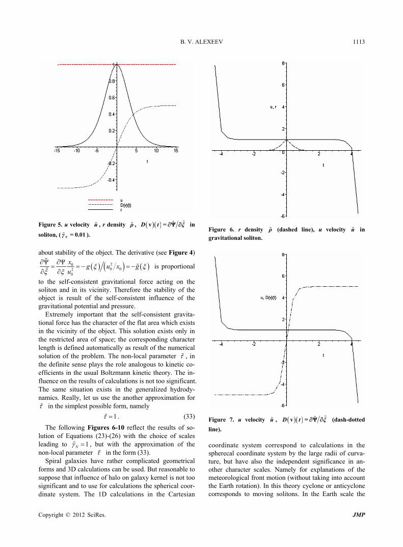
Figures 6-10

3

The following reflect the results of solution of Equations (23)-(26) with the choice of scales leading to 1N , but with the approximation of the non-local parameter in the form (33).

Spiral galaxies have rather complicated geometrical forms and 3D calculations can be used. But reasonable to suppose that influence of halo on galaxy kernel is not too significant and to use for calculations the spherical coordinate system. The 1D calculations in the Cartesian

Figure 6. r density ρ (dashed n in gravitatio on.

li e), u velocity unal solit

Figure 7. u velocity u , v Ψ t = ξ (dash-dotted D

lin

systemradii of curva-

tu

e). coordinate correspond to calculations in the spherecal coordinate system by the large

re, but have also the independent significance in another character scales. Namely for explanations of the meteorological front motion (without taking into account the Earth rotation). In this theory cyclone or anticyclone corresponds to moving solitons. In the Earth scale the


B. V. ALEXEEV 1114

Figu . r density re 8 ρ , u velocity u , w tal velocity w orbi .

G = 0.01 .

Figure 9. p pressure p , v self consistent potential in gravi-

tational soliton, Ψ , v Ψ D t = ξ in gravitational

ales

soliton. sc can be used: 3 31.29air 10 cmg , 0

Figure 10. r density ρ , u velocity u in gravitational soli-

bi

n, w or tal velocity w . G = 1 .

the spherical coordinate system can be found in [29,30]. The following figures reflect the result of soliton calculations for the case of spherical symmetry for galaxy kernel. The velocity u corresponds to the direction of the soliton movement for spherical coordinate system on following figures. Self-consistent gravitational force

to

F acting on the unit of mass permits to define the orbital velocity w of objects in halo, w Fr , or

w rr

, (34)

where r is the distance from the center of galaxy. All calculations are realized for the conditions (SYSTEM I) but for different parameter

2 20 0 0 0N N N NG x u . (35)

Parameter G plays the role of similarity criteria in traditional hydrodynamics. Important conclusions:

Fi

ik urve A on Figurs 14 and 15; large G, like curve B on Figure 1)

r typical spiral galaxies. planets (like Sun) corr

gravitation

l physics in principal and authors of many pa- pe

1) The following gures 8-15 demonstrate evolution of the rotation curves from the Kepler regime (Figures 8 and 9; small G, l e c e 1) to observed (Figurefo

2) The stars with espond to the al soliton with small G and therefore originate

the Kepler rotation regime. 3) Regime B cannot be obtained in the frame of local

1u m s ,

0 10x km and ~ 0.01N . Figure 5 reflects the results of the corresponding calculation and in particular reflects correctly the wind orientation in front and behind of the soliton.

The full system of 3D non-local hydrodynamic equations in moving (along x axis) Cartesian coordinate system and the corresponding expression for derivatives in

statisticars introduce different approximations for additional

“dark matter density” (as usual in Poisson equation) try- ing to find coincidence with data of observations.


B. V. ALEXEEV 1115

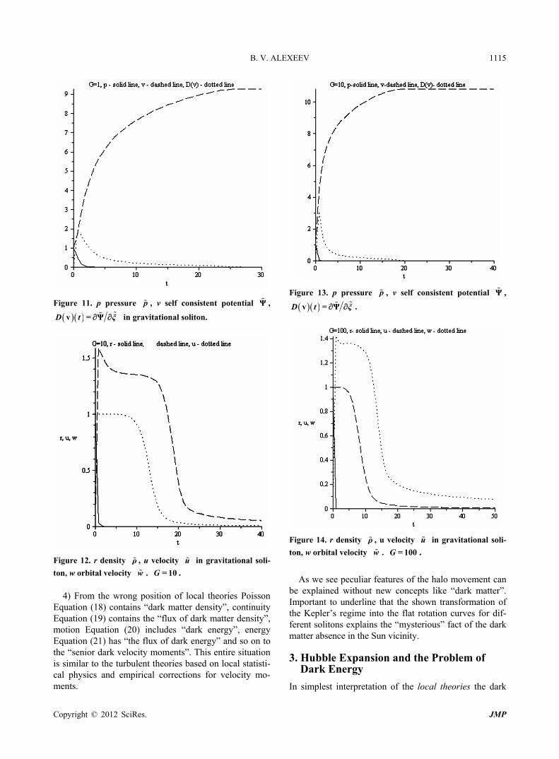
Figure 13. p pressure

p , v self consistent potential ΨFigure 11. p pressur e p , v self c nsistent potential Ψ ,

o

v Ψ D t = ξ in g vi al soliton. ra tation

Figure 12. r density ρ , u velocity u in gravitational soli-

ton, w orbital velocity w . G = 10 .

4) From the wrong position of local theories Poisson Eq

udes “dark energy”, energy Eq

uation (18) contains “dark matter density”, continuity Equation (19) contains the “flux of dark matter density”, motion Equation (20) incl

uation (21) has “the flux of dark energy” and so on to the “senior dark velocity moments”. This entire situation is similar to the turbulent theories based on local statistical physics and empirical corrections for velocity moments.

,

v Ψ D t = ξ .

Figure 14. r density ρ , u velocity u in gravitational sol

.

features of the halo movement can e

lest interpretation of the local theories the dark

i-

ton, w orbital velocity w . G = 100

As we see peculiar

b explained without new concepts like “dark matter”. Important to underline that the shown transformation of the Kepler’s regime into the flat rotation curves for different solitons explains the “mysterious” fact of the dark matter absence in the Sun vicinity.

3. Hubble Expansion and the Problem of Dark Energy

In simp


B. V. ALEXEEV 1116

ssFigure. 15. pre ure p p , v self consi nt potential Ψ , ste

v Ψ= ξ .

energy is related usually to the Einstein cosmological constant. In review [4] the modified Newton force is written as

D t

2

M 8π

3N NF r r

r

v , (36)

where v is the Einstein-Gliner vacuum density [33]. In the limit of large distances the influence of central mass M becomes negligibly small and the field of forces is determined only by the second term in the right side of (36). It follows from relation (36) that there is a distance rv at which the sum of the gravitation and antigravitation forces is equal to zero. I r words rv is “the zero-gravitational radius”. Fo o called Local Group of galaxies ation of rv t 1Mpc.

From the non-local statistical theo e physical pic- ture follows which leading to the Hubble flow witho

rk 36

The main origin of Hubble effect (including the matter ex

to obtain the corre- near eal-

ize rect mathematical model supporting

(USA) and B. Schmidt (Australia). These researchers studied Type 1a supernovae and determined that more distant galactic objects seem to move faster. Their observations suggest that not only is the Universe expanding, its expansion is relentlessly speeding up.

Effects of gravitational self-catching should be typical for Universe. The existence of “Hubble boxes” is discussed in review [4] as typical blocks of the nearby Uni- verse. Gravitational self-catching takes place for Big Bang having given birth to the global expansion of Uni- verse, but also for Little Bang in so called Local Group (using the Hubble’s terminology) of galaxies. Then the evolution of the Local Group (the typical Hubble box) is really fruitful field for testing of different theoretical constructions (see Figure 16). The data were obtained by Karachentsev and his collaborators in 2002-2007 in ob-servation with the Hubble Space Telescope [4,32]. Each point corresponds to a galaxy with measured values of distance and line-of-site velocity in the reference fram

shows two distinct structures, the Local Group and the

cal flow of galaxies. The galaxies of the Local Group

(positive velocities) and toward the center (negative velocities). These galaxies formally bound quasi-stationary system. Thvelocity is equal to zero. The galaxies of the local flow

n other s

is aboury th

estim

utnew essence like da energy and without modification of Newton force like ( ).

Namely:

pansion with acceleration) is self—catching of expanding matter by the self—consistent gravitational field in conditions of weak influence of the central massive bodies.

The formulated result is obtained in the frame of the linear theory [25,31]. Is it possiblesponding result on the level of the general non-lidescription? Such an investigation was successfully r

d and leads to a dithe well known observations of S. Perlmutter, A. Riess

e related to the center of the Local Group. The diagram

looccupy a volume with the radius up to ~1.1 - 1.2 Mpc, but there are no galaxies in the volume whose radius is less than 0.25 Mpc. These galaxies move both away from the center

a gravitation- eir average radial

are located outside the group and all of them are moving from the center (positive velocities) beginning their motion near 1 MpcR with the velocity ~ 50 km/sv . By the way the measured by Karachentsev the average Hubble parameter for the Local Group is 72 ± 6

1 1km s Mpc . Let us choose these values as scales:

0 01 Mpc, 50 km/sx u . (37)

Recession velocities increase as the distance increases in accordance with the Hubble law. The straight line correspond the dependence from observations

r r (38)

fo

v H

r the region outside of the Local Group. In the non- dimensional form

v H r r (39)

where

0

0

xH H r

u . (40)

For the following calculations we should choose the corresponding scales (especially for estimating G ) for modeling of the Local Group evolution


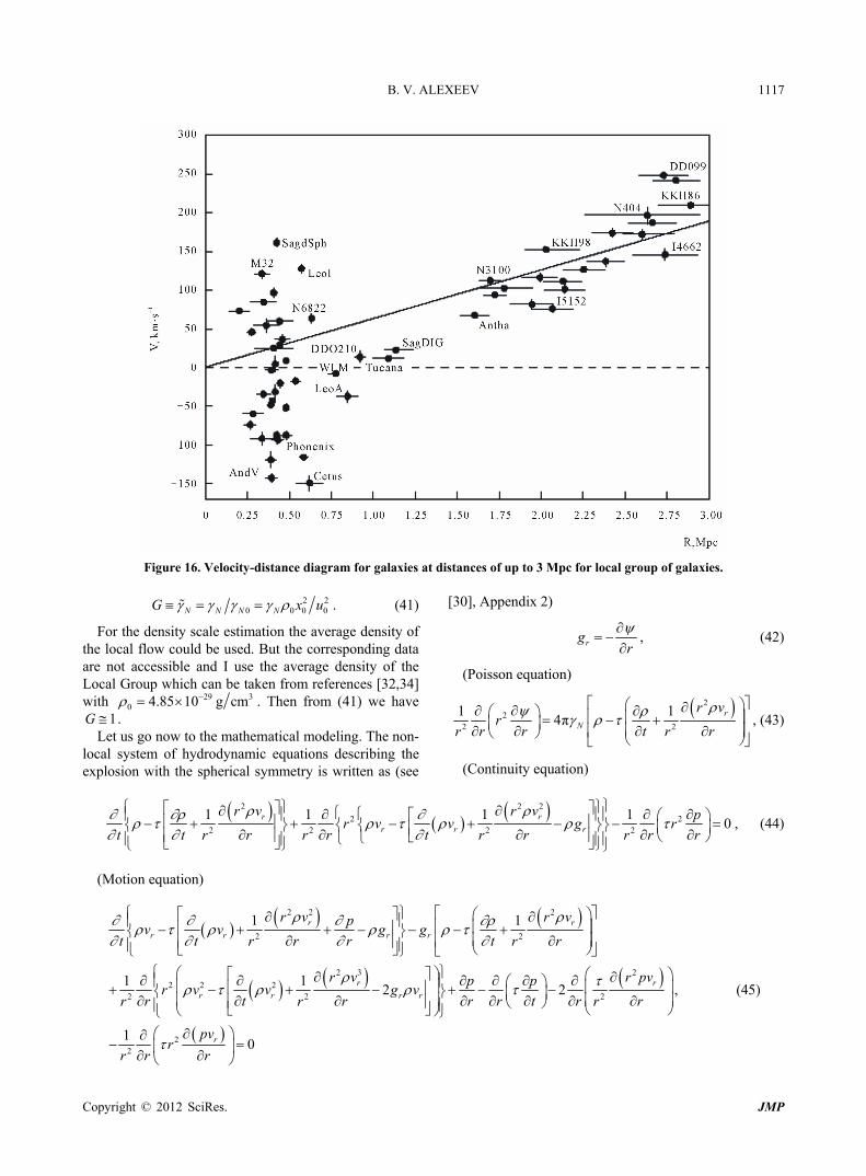
B. V. ALEXEEV

JMP

1117

tances of up to 3 Mpc for local group of galaxies. Figure 16. Velocity-distance diagram for galaxies at

dis

2 20 0 0 0N N N NG x u . (41)

Copyright © 2012 SciRes.

For the density scale estimthe local flow could be used.

ation the average density of But the corresponding data

are not accessible and I use the average density of the Local Group which can be taken from references [32,34] with 29 3

0 4.85 10 g cm . Then from (41) we have G

to the mathematical modeling. The non- drodynamic equations describing the

explosion with the spherical symmetry is written as (see

[30], Appendix 2)

1. Let us go now

local system of hy

rgr

, (42)

(Poisson equation)

2

22 2

1 14π

r

N

r vr

r r t rr r

, (43)


2 2 2

2 22 2 2 2

1 1 1 10

r r

r r r

r v r v pr v v g r

t t r r t r r rr r r r

, (44)

(M ) otion equation

2 2 2

2 2

2 3 2

2 2 2

1 1

2 2

r r

r r

r r

r r r r

r v r vpg g

r r t rr r

r v r pvp pg v

r t r r r t r rr r r

2 2 21 1

r rv vt t

r v v

21 rpv

r2 0rr r

, (45)

B. V. ALEXEEV 1118

(Energy equation)

2 22

2 2 22

1 3 1 3 1

2 2 2 2

1 1 5 1

2 2

r r

r r r

v p v pt t rr

r v p v vr r

2 2

2 22

1 5

2 2

5 7

2 2 2 2

1

r r r r

r r r

r v v p g v

p v p vr t r

21 1v r

2 2

2r r rg v v

2

2 2 2

2

1 1 5 1

r r rp g g v

pr pv r p

2 22

2 2

3 1

2 2

r r r r

r r

pg v r v g

t r rr

gr r rr r

0.

The system of Equations (43)-(46) belongs to the class of the 1D non-stationary equations and can be solved by kn thods. But for the aims of the trans-pa cal modeling of self-catching of the expanding matter by the self-consistent gravitational field I introduce the following assumption. Let us allot the quasi-stationary Hubble regime when only the im-plicit dependence on time for the unknown values exists. It means that for the intermediate (Hubble) regime the

substitution

(46)

own numerical merent vast mathemati

r

rv

t r t r

(47)

can be introduced. As result we have the following system of the 1D dimensionless equations:

2

22 2

1 14π

r

r

r vr G v

r r r rr r

,(48)

2

2

2 2

22 2

1

1 1 10,

r

r r

r

r r

r vv v

r r rr

r v pv v r

r r r r rr r

(49)

22 rr v

rr

2 2 2

2

1 1r r

r

r v r vpv v v v v

r r rr r

2

2 3

2 2 22 2

1 12

r r r r

r

r r r

r r r r r

r vr v v v v

r r r rr r

2

22 2

12 0

r

r rr

r pv pvp pv r

r r r r r r rr r

,

(50)

2 2 2 22

2 2 22 2

13 3 2

1 15 5

r r r r r r

r r r r r

v v p v v p r v v pr r rr

r v p v v v p vr rr r

2 2 2 2 27 2 3r r r rr v p v v v pr r r

5 rvr

2 22

22 2 2

12

1 15 2 0

r r r r

pv v v r v

r r r r rr

pr pv r p

2 2r

r

r r r rr r

(51)


B. V. ALEXEEV 1119

The system of generalized hydrodynamic equations

(48)-(51) have the great possibilities of mathematical modeling as result of changing of eight Cauchy conditions describing the character features of the local flow evolution. The following Maple notations on figures are use —density d: r velocity rv —pressure p and —self consistent

, u— , pv potential , h — H and inde-

pend iable t nations placed under all fo igures, e prog m cont Maple’s no-

p 0 0D u means in

enllowing

the us

t var f

tations—for exam

is Mapl

rl. Expla

ra ains e the expression

ual notations 0 0 . n- meter

u r noAs mentioned before, the local para , in

the definite sense plays the role an ous to kinetic co- efficients in the usual Boltzmann kinetic theory. The influence on the results of calcula gnificant, (see (31, 33)). The same situa generalized hydrodynamics. As before I introduce the following approximation for the dimensionless n-local parameter

ru v )

alog

tions is not too sition exists in the

no(see (31), here 21 u define also the

tion for the quasi-stationary regime

. Let us celeration funcdimensionless acceleration-de

Figure 17. Dependence of the acceleration-deceleration function Q (in Maple notation D u t = u r ), deriva-

tion of the self-consistent potential rv uQ

r r

, (52)

as an analogue of the dimensionless deceleration function q which was used in [28].

One obtains for the approximation (31) and SYSTEM 2:

v Ψ D t = ξ and

velocity u = u on the radial distance r .

v 1 = 1, u 1 = 1, r 1 = 1, p 1 = 1 , D v 1 = 0 , .

= 1. From these calculations follow:

) As it was waiting the quasi-stationary regime exists on

sh F or-ce ct al

D uFigures

= 0 , 17 and

1 D r 1 = 0 18 corresp

, D p 1 = 0ond to G

1ly in the restricted (on the left and on the right sides)

area. Out of these boundaries the explicit time dependent regime should be considered. But it is not the Hubble regime.

2) In the Hubble regime one obtains the negative area (low part of the da -dotted curve of igure 17). It c responds to the self-consistent for a ing ong the expansion of the local flow.

3) The dependence of H r is not linear (see Figure 18), more over the curvature cont m. The area of acceleration pl

ains maximuaced between two areas of the de-

y the 0

celeration. Let us show now the result of calculations for another

approximation in the simplest possible form, namely (see also (33)) 1 . One obtains for this - approximation and SYSTEM 2 for G = 1, see Figures 19-22.

We can add to the previous conclusions: 4) Approximation const conserves all principal

characters of the previous dependences, but the area of the Hubble regime becomes larger.

5) Approximation

Figure 18. Dependence of the dimensionless Hubble pa-rameter on the radial distance. numerical transition to the “classical” gas dynamics of explosions. B there are no Hubble regimes in

istent gravitational field.

principal. 6) Diminishing of G leads to diminishing of the area of

the Hubble regime with the positive acceleration of the matter catched by the self-cons

7) Dependence of H r do es not contain the maxi- const allows realizing the


B. V. ALEXEEV 1120

Figure 19. r density ρ , u u , v Ψ D t = ξ .

Figure 20. Dependence of the acceleration-deceleration

D u t

Figure 21. Dependence of the dimensionless Hubble pa-rameter on the radial distance for G = 1.

Figure 22. Dependence of the dimensionless hubble parameter on the radial distance for G = 10. the rotational speeds of galaxies and the Hubble expansion with acceleration need not in the introduction of new essence like dark matter and dark energy.

4. Conclusion

The n o heory is applied for athematical modeling of cosmic objects with success.

case of galaxies the theory leads to the flat rotation curves known from observations. The transformation

= u r on r .

mum on the curve for the small value of parameter G (A- regime). It is reasonable to find from the observation the Hubble boxes where A-regime is realizing. Considera- tion of the Local Group evolution of galaxies (see Figure 16) leaves the impression that this burst responds to the PRS-regime.

As we see the Hubble expansion with acceleration is explained as result of mathematical modeling based on the principles of non-local physics. Peculiar features of

unified generalized on-l cal tmFor the


B. V. ALEXEEV 1121

of Kepler’s regime into the flat rotation curves for different solitons is shown. The origin of Hubble effect (in-cluding the matter expansion with acceleration) is self- catching of the expanding matter by the self-consistent gravitational field in conditions of weak influence of the central massive bodies. The Hubble expansion with acceleration is obtained as result of mathematical modeling based on the principles of non-local physics. Peculiar features of the rotational speeds of galaxies and effects of the Hubble expansion need not in the introduction of new essence like dark matter and dark energy. The origin of difficulties consists in the total Oversimplification following from the principles of local physics.

REFERENCES

[1] V. Rubin and W. K. Ford Jr., “Rotation of the Andromeda Nebula from a Spectroscopic Survey of Emission Re

doi:10.1086 7

- gions,” Astrophysical Journal, Vol. 159, 1970, p. 379.

/15031

[2] V. Rubin, N. Thonnard and W. K. Ford Jr., “Rotational Properties of 21 Sc Galaxies with a Large Range of Lu- minosities and Radii from NGC 4605 (R = 4 kpc) to UGC 2885 (R = 122 kpc),” Astrophysical Journal, Vol. 238, 1980, pp. 471-487. doi:10.1086/158003

[3] M. Milgrom, “The MOND Paradigm,” ArXiv Preprint, 2007. http://arxiv.org/abs/0801.3133v2

[4] A. D. Chernin, “Dark Energy and Universal Antigravita- tion,” Physics-Uspekhi, Vol. 51, No. 3, 2008, pp. 267-300. doi:10.1070/PU2008v051n03ABEH006320

[5] J. S. Bell, “On the Einstein Podolsky Rosen Paradox,” Physics, No. 1, 1964, pp. 195-200.

[6] B. V. Alexeev, “Generalized Boltzmann Physical Kinet- ics,” Elsevier, Amsterdam, 2004.

[7] L. Boltzmann. “Weitere Studien über das Warmegleich- gewicht unter Gasmoleculen,” Sitzungsberichte der Kai- serlichen Akademie der Wissenschaften, Vol. 66, 1872, p. 275.

[8] L. Boltzmann, “Vorlesungen über Gastheorie,” Verlag von Johann Barth, Zweiter Unveränderten Abdruck. 2 Teile, Leipzig, 1912.

[9] N. N. Bogolyubov, “Problemy Dinamicheskoi Teorii v Statisticheskoi Fizike, (Dynamic Theory Problems in Sta- tistical Physics),” Moscow Leningrad Gostekhizdat, 1946.

[10] M. Born and H. S. Green. “A General Kinetic Theory of Liquids,” Proceedings of the Royal Society, Vol. 188, No. 1012, 1946, pp. 10-18. doi:10.1098/rspa.1946.0093

[11] H. S. Green, “The Molecular Theory of Fluids,” North- Holland, Amsterdam, 1952.

[12] J. G. Kirkwood, “The Statistical Mechanical Theor Transport Processes 2: Transport in Gases,” Journal of

y of

Chemical Physics, Vol. 15, No. 1, 1947, pp. 72-76. doi:10.1063/1.1746292

[13] J. Yvon, “La Theorie Statistique des Fluides et l’Equationd’etat,” Hermann, Paris, 1935.

[14] B. V. Alekseev, “Matematicheskaya Kinetika Reagiru- yushchikh Gazov,” (Mathematical Theory of Reacting Gases), Nauka, Moscow, 1982.

[15] B. V. Alexeev, “The Generalized Boltzmann Equation, Generalized Hydrodynamic Equations and their Applica- tions,” Philosophical Transactions of the Royal Society of London, Vol. 349, 1994, pp. 417-443. doi:10.1098/rsta.1994.0140

[16] B. V. Alexeev, “The Generalized Boltzmann Equation,” Physica A, Vol. 216, No. 4, 1995, pp. 459-468. doi:10.1016/0378-4371(95)00044-8

[17] S. Chapman and T. G. Cowling, “The Mathematical The- ory of Non-Uniform Gases,” University Press, Cambridge, 1952.

[18] I. O. Hirschfelder, Ch. F. Curtiss and R. B. Bird, “Mo-lecular Theory of Gases and Liquids,” John Wiley and sons, Inc., New York, Chapman and Hall, London, 1954.

[19] Yu. L. Klimontovich, “About Necessity and Possibility of Unified Description of Hydrodynamic Processes,” Theo- retical and Mathematical Physics, Vol. 92, No. 2, 1992, p. 312.

Physics-Uspekhi, Vol. 43, No. 6, 2000, pp. 601-629.

[20] B. V. Alekseev, “Physical Basements of the Generalized Boltzmann Kinetic Theory of Gases,”

doi:10.1070/PU2000v043n06ABEH000694

[21] B. V. Alekseev, “Physical Fundamentals of the General- ized Boltzmann Kinetic Theory of Ionizeics-Uspekhi, Vol. 46, No. 2, 2003, pp. 139

d Gases,” Phys- -167.

2003v046n02ABEH001221doi:10.1070/PU

[22] B. V. Alexeev, “Generalized Quantum Hydrodynamics and Principles of Non-Local Physics,” Journal of Nano- electronics and Optoelectronics, Vol. 3, No. 2, 2008, pp. 143-158. doi:10.1166/jno.2008.207

[23] B. V. Alexeev, “Application of Generalized Quantum Hydrodynamics in the Theory of Quantum Soliton Evolu- tion,” Journal of Nanoelectronics and Optoelectronics, Vol. 3, No. 3, 2008, pp. 316-328. doi:10.1166/jno.2008.311

[24] B. V. Alexeev, “Generalized Theory of Landau Damp- ing,” Journal of Nanoelectronics and Optoelectronics, Vol. 4, No. 1, 2009, pp. 186-199. doi:10.1166/jno.2009.1021

[25] B. V. Alexeev, “Generalized Theory of Landau Damping in Collisional Media,” Journal of Nanoelectronics and Optoelectronics, Vol. 4, No. 3, 2009, pp. 379-393. doi:10.1166/jno.2009.1054

[26] S. Perlmutter, et al., “Measurements of Ω and Λ from 42 High-Redshift Supernovae,” Astrophysical Journal, Vol. 517, No. 2, 1999, pp. 565-586. doi:10.1086/307221

[27] A. G. Riess, et al., “Observational Evidence from Super- novae for an nd a Cosmological Constant,” As . 116, No. 3, 1998,

Accelerating Universe atronomical Journal, Vol

pp. 1009-1038. doi:10.1086/300499

[28] A. G. Riess, et al., “Type IA Supernova Discoveries at 1z from the Hubble Telescope: Evidence for Past D

celeration and Conste-

raints on Dark Energy Evolution,” Astrophysical Journal, Vol. 607, 2004, pp. 665-687. doi:10.1086/383612


B. V. ALEXEEV


1122

Non-Local Phys-Medium and

es in the ersity Press,

[29] B. V. Alexeev, “Non-local Physics. Non-Relativistic The- ory,” Lambert Academic Press (in Russian), 2011.

[30] B. V. Alexeev and I. V. Ovchinnikova, “

Loca

ics. Relativistic Theory,” Lambert Academic Press, 2011, (in Russian).

[31] B. V. Alexeev, “Application of Non-Local Physics in the Theory of Hubble Expansion,” Nova Science Publishers, Inc., 2011.

[32] I. D. Karachentsev and O. G. Kashibadze, “Masses of the

l Group and of the M81 Group Estimated from Dis-tortions in the Local Velocity Field,” Astrophysics, Vol. 49, No. 1, 2006, pp. 3-18.

[33] E. B. Gliner, “The Vacuum-Like State of a Friedman Cosmology,” Soviet Physics—Doklady, Vol. 15, No. 6, 1970, pp. 559-561.

[34] L. S. Sparke and J. S. Gallagher III, “GalaxiUniverse: Introduction,” Cambridge UnivCambridge, 2000.

to the theory of galaxies rotation and the hubble

Documents