tìm kiếm trên đồ thị (version 0.2) - thangdn.com filechú ý: nhiều hình vẽ trong tài...
TRANSCRIPT
Tìm kiếm trên đồ thị (Version 0.2)
Trần Vĩnh Đức
HUST
Ngày 20 tháng 4 năm 2017
1 / 57

Tài liệu tham khảo
▶ S. Dasgupta, C. H. Papadimitriou, and U. V. Vazirani,Algorithms, July 18, 2016.
▶ Chú ý: Nhiều hình vẽ trong tài liệu được lấy tùy tiện mà chưaxin phép.
2 / 57

Nội dung
Biểu diễn đồ thị
Tìm kiếm theo chiều sâu trên đồ thị vô hướng
Tìm kiếm theo chiều sâu trên đồ thị có hướng
Thành phần liên thông mạnh

Biểu diễn đồ thị dùng Ma trận kềNếu đồ thị có n = |V| đỉnh v1, v2, . . . , vn, thì ma trận kề là mộtmảng n × n với phần tử (i, j) của nó là
aij =
{1 nếu có cạnh từ vi tới vj
0 ngược lại.
Ví dụ
v1
v2
v3
A =
1 1 10 0 10 1 0
4 / 57

Dùng ma trận kề có hiệu quả?
▶ Có thể kiểm tra có cạnh nối giữa cặp đỉnh bất kỳ chỉ cần mộtlần truy cập bộ nhớ.
▶ Tuy nhiên, không gian lưu trữ là O(n2)
5 / 57

Biểu diễn đồ thị dùng danh sách kề▶ Dùng một mảng Adj gồm |V| danh sách.▶ Với mỗi đỉnh u ∈ V, phần tử Adj[u] lưu trữ danh sách các
hàng xóm của u. Có nghĩa rằng:
Adj[u] = {v ∈ V | (u, v) ∈ E}.
Ví dụ
0
1
2
Adj[0] = {0, 1, 2}Adj[1] = {2}Adj[2] = {1}
6 / 57

Dùng danh sách kề có hiệu quả?
▶ Có thể liệt kê các đỉnh kề với một đỉnh cho trước một cáchhiệu quả.
▶ Nó cần không gian lưu trữ là O(|V|+ |E|). Ít hơn O(|V|2) rấtnhiều khi đồ thị ít cạnh.
7 / 57

Nội dung
Biểu diễn đồ thị
Tìm kiếm theo chiều sâu trên đồ thị vô hướng
Tìm kiếm theo chiều sâu trên đồ thị có hướng
Thành phần liên thông mạnh

ptg12441863
Adjacency-lists data structure. adjacency-lists data structure
Bag Section 1.3 --
Graph
tinyG.txt v and w, we add w to vlist and v to w twiceGraph
n V + E n
n v v
Note
Graph -
Graphadj()
-Graph
toString()-
Exercise 4.1.7
13130 54 30 19 126 45 40 211 129 100 67 89 115 3
% java Graph tinyG.txt13 vertices, 13 edges0: 6 2 1 5 1: 0 2: 0 3: 5 4 4: 5 6 3 5: 3 4 0 6: 0 4 7: 8 8: 7 9: 11 10 12 10: 911: 9 12 12: 11 9
tinyG.txt
Output for list-of-edges input
VE
first adjacentvertex in input
is last on list
secondrepresentation
of each edgeappears in red
5254.1 n Undirected Graphs
Câu hỏiTừ một đỉnh của đồ thị ta có thể đi tới những đỉnh nào?
9 / 57

Tìm đường trong mê cung
P1: OSO/OVY P2: OSO/OVY QC: OSO/OVY T1: OSO
das23402 Ch03 GTBL020-Dasgupta-v10 August 10, 2006 19:18
Chapter 3 Algorithms 83
Figure 3.2 Exploring a graph is rather like navigating a maze.
A
C
B
F
D
H I J
K
E
G
L
H
G
DA
C
FKL
J
I
B
E
3.2 Depth-first search in undirected graphs3.2.1 Exploring mazesDepth-first search is a surprisingly versatile linear-time procedure that reveals awealth of information about a graph. The most basic question it addresses is,
What parts of the graph are reachable from a given vertex?
To understand this task, try putting yourself in the position of a computer that hasjust been given a new graph, say in the form of an adjacency list. This representationoffers just one basic operation: finding the neighbors of a vertex. With only thisprimitive, the reachability problem is rather like exploring a labyrinth (Figure 3.2).You start walking from a fixed place and whenever you arrive at any junction (vertex)there are a variety of passages (edges) you can follow. A careless choice of passagesmight lead you around in circles or might cause you to overlook some accessiblepart of the maze. Clearly, you need to record some intermediate information duringexploration.
This classic challenge has amused people for centuries. Everybody knows that allyou need to explore a labyrinth is a ball of string and a piece of chalk. The chalkprevents looping, by marking the junctions you have already visited. The stringalways takes you back to the starting place, enabling you to return to passages thatyou previously saw but did not yet investigate.
How can we simulate these two primitives, chalk and string, on a computer? Thechalk marks are easy: for each vertex, maintain a Boolean variable indicatingwhether it has been visited already. As for the ball of string, the correct cyber-analog is a stack. After all, the exact role of the string is to offer two primitiveoperations—unwind to get to a new junction (the stack equivalent is to push thenew vertex) and rewind to return to the previous junction (pop the stack).
Instead of explicitly maintaining a stack, we will do so implicitly via recursion(which is implemented using a stack of activation records). The resulting algorithm
Hình: Tìm kiếm trên đồ thị cũng giống tìm đường trong mê cung
10 / 57

procedure explore(G, v)Input: đồ thị G = (V,E); v ∈ VOutput: visited(u)=true với mọi đỉnh u có thể đếnđược từ v
visited(v) = trueprevisit(v)for each edge (v, u) ∈ E:
if not visited(u): explore(G, u)postvisit(v)
11 / 57

Ví dụ: Kết quả chạy explore(A)
P1: OSO/OVY P2: OSO/OVY QC: OSO/OVY T1: OSO
das23402 Ch03 GTBL020-Dasgupta-v10 August 10, 2006 19:18
Chapter 3 Algorithms 83
Figure 3.2 Exploring a graph is rather like navigating a maze.
A
C
B
F
D
H I J
K
E
G
L
H
G
DA
C
FKL
J
I
B
E
3.2 Depth-first search in undirected graphs3.2.1 Exploring mazesDepth-first search is a surprisingly versatile linear-time procedure that reveals awealth of information about a graph. The most basic question it addresses is,
What parts of the graph are reachable from a given vertex?
To understand this task, try putting yourself in the position of a computer that hasjust been given a new graph, say in the form of an adjacency list. This representationoffers just one basic operation: finding the neighbors of a vertex. With only thisprimitive, the reachability problem is rather like exploring a labyrinth (Figure 3.2).You start walking from a fixed place and whenever you arrive at any junction (vertex)there are a variety of passages (edges) you can follow. A careless choice of passagesmight lead you around in circles or might cause you to overlook some accessiblepart of the maze. Clearly, you need to record some intermediate information duringexploration.
This classic challenge has amused people for centuries. Everybody knows that allyou need to explore a labyrinth is a ball of string and a piece of chalk. The chalkprevents looping, by marking the junctions you have already visited. The stringalways takes you back to the starting place, enabling you to return to passages thatyou previously saw but did not yet investigate.
How can we simulate these two primitives, chalk and string, on a computer? Thechalk marks are easy: for each vertex, maintain a Boolean variable indicatingwhether it has been visited already. As for the ball of string, the correct cyber-analog is a stack. After all, the exact role of the string is to offer two primitiveoperations—unwind to get to a new junction (the stack equivalent is to push thenew vertex) and rewind to return to the previous junction (pop the stack).
Instead of explicitly maintaining a stack, we will do so implicitly via recursion(which is implemented using a stack of activation records). The resulting algorithm
P1: OSO/OVY P2: OSO/OVY QC: OSO/OVY T1: OSO
das23402 Ch03 GTBL020-Dasgupta-v10 August 10, 2006 19:18
Chapter 3 Algorithms 85
Figure 3.4 The result of explore(A) on the graph of Figure 3.2.
I
E
J
C
F
B
A
D
G
H
For instance, while B was being visited, the edge B − E was noticed and, since Ewas as yet unknown, was traversed via a call to explore(E ). These solid edgesform a tree (a connected graph with no cycles) and are therefore called tree edges.The dotted edges were ignored because they led back to familiar terrain, to verticespreviously visited. They are called back edges.
3.2.2 Depth-first searchThe explore procedure visits only the portion of the graph reachable from itsstarting point. To examine the rest of the graph, we need to restart the procedureelsewhere, at some vertex that has not yet been visited. The algorithm of Figure 3.5,called depth-first search (DFS), does this repeatedly until the entire graph has beentraversed.
Figure 3.5 Depth-first search.
procedure dfs(G)
for all v ∈ V:visited(v) = false
for all v ∈ V:if not visited(v): explore(v)
The first step in analyzing the running time of DFS is to observe that each vertex isexplore’d just once, thanks to the visited array (the chalk marks). During theexploration of a vertex, there are the following steps:
1. Some fixed amount of work—marking the spot as visited, and thepre/postvisit.
12 / 57
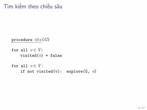
Tìm kiếm theo chiều sâu
procedure dfs(G)
for all v ∈ V:visited(v) = false
for all v ∈ V :if not visited(v): explore(G, v)
13 / 57

Ví dụ: Đồ thị và Rừng DFS
P1: OSO/OVY P2: OSO/OVY QC: OSO/OVY T1: OSO
das23402 Ch03 GTBL020-Dasgupta-v10 August 10, 2006 19:18
86 3.2 Depth-first search in undirected graphs
2. A loop in which adjacent edges are scanned, to see if they lead somewherenew.
This loop takes a different amount of time for each vertex, so let’s consider allvertices together. The total work done in step 1 is then O(|V |). In step 2, overthe course of the entire DFS, each edge {x, y} ∈ E is examined exactly twice, onceduring explore(x) and once during explore(y). The overall time for step 2 istherefore O(|E |) and so the depth-first search has a running time of O(|V | + |E |),linear in the size of its input. This is as efficient as we could possibly hope for, sinceit takes this long even just to read the adjacency list.
Figure 3.6 (a) A 12-node graph. (b) DFS search forest.
(a)
A B C D
E F G H
I J K L
(b) A
B E
I
J G
K
FC
D
H
L
1,10
2,3
4,9
5,8
6,7
11,22 23,24
12,21
13,20
14,17
15,16
18,19
Figure 3.6 shows the outcome of depth-first search on a 12-node graph, once againbreaking ties alphabetically (ignore the pairs of numbers for the time being). Theouter loop of DFS calls explore three times, on A, C , and finally F . As a result,there are three trees, each rooted at one of these starting points. Together theyconstitute a forest.
3.2.3 Connectivity in undirected graphsAn undirected graph is connected if there is a path between any pair of vertices. Thegraph of Figure 3.6 is not connected because, for instance, there is no path from Ato K . However, it does have three disjoint connected regions, corresponding to thefollowing sets of vertices:
{A, B, E , I , J } {C , D, G , H, K , L} {F }.
These regions are called connected components: each of them is a subgraph that isinternally connected but has no edges to the remaining vertices. When exploreis started at a particular vertex, it identifies precisely the connected componentcontaining that vertex. And each time the DFS outer loop calls explore, a newconnected component is picked out.
14 / 57

Bài tậpXây dựng rừng DFS cho đồ thị sau. Vẽ cả những cạnh nét đứt.
15 / 57

Rừng DFS và số thành phần liên thông
P1: OSO/OVY P2: OSO/OVY QC: OSO/OVY T1: OSO
das23402 Ch03 GTBL020-Dasgupta-v10 August 10, 2006 19:18
86 3.2 Depth-first search in undirected graphs
2. A loop in which adjacent edges are scanned, to see if they lead somewherenew.
This loop takes a different amount of time for each vertex, so let’s consider allvertices together. The total work done in step 1 is then O(|V |). In step 2, overthe course of the entire DFS, each edge {x, y} ∈ E is examined exactly twice, onceduring explore(x) and once during explore(y). The overall time for step 2 istherefore O(|E |) and so the depth-first search has a running time of O(|V | + |E |),linear in the size of its input. This is as efficient as we could possibly hope for, sinceit takes this long even just to read the adjacency list.
Figure 3.6 (a) A 12-node graph. (b) DFS search forest.
(a)
A B C D
E F G H
I J K L
(b) A
B E
I
J G
K
FC
D
H
L
1,10
2,3
4,9
5,8
6,7
11,22 23,24
12,21
13,20
14,17
15,16
18,19
Figure 3.6 shows the outcome of depth-first search on a 12-node graph, once againbreaking ties alphabetically (ignore the pairs of numbers for the time being). Theouter loop of DFS calls explore three times, on A, C , and finally F . As a result,there are three trees, each rooted at one of these starting points. Together theyconstitute a forest.
3.2.3 Connectivity in undirected graphsAn undirected graph is connected if there is a path between any pair of vertices. Thegraph of Figure 3.6 is not connected because, for instance, there is no path from Ato K . However, it does have three disjoint connected regions, corresponding to thefollowing sets of vertices:
{A, B, E , I , J } {C , D, G , H, K , L} {F }.
These regions are called connected components: each of them is a subgraph that isinternally connected but has no edges to the remaining vertices. When exploreis started at a particular vertex, it identifies precisely the connected componentcontaining that vertex. And each time the DFS outer loop calls explore, a newconnected component is picked out.
v ccnum[v]A 1B 1C 2D 2E 1F 3G 2H 2I 1J 1
Biến ccnum[v] để xác định thành phần liên thông của đỉnh v.
16 / 57

Tính liên thông trong đồ thị vô hướngprocedure dfs(G)cc = 0for all v ∈ V: visited(v) = falsefor all v ∈ V:
if not visited(v):cc = cc + 1explore(G, v)
procedure explore(G, v)visited(v) = trueprevisit(v)for each edge (v, u) ∈ E:
if not visited(u): explore(G, u)postvisit(v)
procedure previsit(v)ccnum[v] = cc
17 / 57

Bài tậpHãy cài đặt chương trình tính số thành phần liên thông của mộtđồ thị vô hướng.
18 / 57
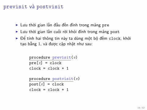
previsit và postvisit
▶ Lưu thời gian lần đầu đến đỉnh trong mảng pre▶ Lưu thời gian lần cuối rời khỏi đỉnh trong mảng post▶ Để tính hai thông tin này ta dùng một bộ đếm clock, khởi
tạo bằng 1, và được cập nhật như sau:
procedure previsit(v)pre[v] = clockclock = clock + 1
procedure postvisit(v)post[v] = clockclock = clock + 1
19 / 57

Bài tậpVẽ rừng DFS với cả số pre và post cho mỗi đỉnh cho đồ thị sau.
20 / 57

Tính chất của previsit và postvisit
Mệnh đềVới mọi đỉnh u và v, hai khoảng
[ pre(u), post(u) ] và [ pre(v), post(v) ]
▶ hoặc là rời nhau,▶ hoặc là có một khoảng chứa một khoảng khác.
Tại sao? vì [ pre(u), post(u) ] là khoảng thời gian đỉnh u nằmtrong ngăn xếp. Cấu trúc vào-sau, ra-trước đảm bảo tính chất này.
21 / 57

Nội dung
Biểu diễn đồ thị
Tìm kiếm theo chiều sâu trên đồ thị vô hướng
Tìm kiếm theo chiều sâu trên đồ thị có hướng
Thành phần liên thông mạnh

Bài tậpHãy vẽ rừng DFS với số pre và post trên mỗi đỉnh cho đồ thị cóhướng sau.
P1: OSO/OVY P2: OSO/OVY QC: OSO/OVY T1: OSO
das23402 Ch03 GTBL020-Dasgupta-v10 August 10, 2006 19:18
88 3.3 Depth-first search in directed graphs
Figure 3.7 DFS on a directed graph.
AB C
F DE
G H
A
H
B C
E D
F
G
12,15
13,14
1,16
2,11
4,7
5,6
8,9
3,10
In further analyzing the directed case, it helps to have terminology for importantrelationships between nodes of a tree. A is the root of the search tree; everythingelse is its descendant. Similarly, E has descendants F , G , and H , and conversely,is an ancestor of these three nodes. The family analogy is carried further: C is theparent of D, which is its child.
For undirected graphs we distinguished between tree edges and nontree edges. Inthe directed case, there is a slightly more elaborate taxonomy:
Bac
k
Forward
Cross
Tree
A
B
C D
DFS treeTree edges are actually part of the DFS forest.
Forward edges lead from a node to a nonchild descendant inthe DFS tree.
Back edges lead to an ancestor in the DFS tree.
Cross edges lead to neither descendant nor ancestor; theytherefore lead to a node that has already been completelyexplored (that is, already postvisited).
Figure 3.7 has two forward edges, two back edges, and two cross edges. Can youspot them?
Ancestor and descendant relationships, as well as edge types, can be read off directlyfrom pre and post numbers. Because of the depth-first exploration strategy, vertexu is an ancestor of vertex v exactly in those cases where u is discovered first and
23 / 57

DFS trên đồ thị có hướng
P1: OSO/OVY P2: OSO/OVY QC: OSO/OVY T1: OSO
das23402 Ch03 GTBL020-Dasgupta-v10 August 10, 2006 19:18
88 3.3 Depth-first search in directed graphs
Figure 3.7 DFS on a directed graph.
AB C
F DE
G H
A
H
B C
E D
F
G
12,15
13,14
1,16
2,11
4,7
5,6
8,9
3,10
In further analyzing the directed case, it helps to have terminology for importantrelationships between nodes of a tree. A is the root of the search tree; everythingelse is its descendant. Similarly, E has descendants F , G , and H , and conversely,is an ancestor of these three nodes. The family analogy is carried further: C is theparent of D, which is its child.
For undirected graphs we distinguished between tree edges and nontree edges. Inthe directed case, there is a slightly more elaborate taxonomy:
Bac
k
Forward
Cross
Tree
A
B
C D
DFS treeTree edges are actually part of the DFS forest.
Forward edges lead from a node to a nonchild descendant inthe DFS tree.
Back edges lead to an ancestor in the DFS tree.
Cross edges lead to neither descendant nor ancestor; theytherefore lead to a node that has already been completelyexplored (that is, already postvisited).
Figure 3.7 has two forward edges, two back edges, and two cross edges. Can youspot them?
Ancestor and descendant relationships, as well as edge types, can be read off directlyfrom pre and post numbers. Because of the depth-first exploration strategy, vertexu is an ancestor of vertex v exactly in those cases where u is discovered first and
24 / 57

Các kiểu cạnh
P1: OSO/OVY P2: OSO/OVY QC: OSO/OVY T1: OSO
das23402 Ch03 GTBL020-Dasgupta-v10 August 10, 2006 19:18
88 3.3 Depth-first search in directed graphs
Figure 3.7 DFS on a directed graph.
AB C
F DE
G H
A
H
B C
E D
F
G
12,15
13,14
1,16
2,11
4,7
5,6
8,9
3,10
In further analyzing the directed case, it helps to have terminology for importantrelationships between nodes of a tree. A is the root of the search tree; everythingelse is its descendant. Similarly, E has descendants F , G , and H , and conversely,is an ancestor of these three nodes. The family analogy is carried further: C is theparent of D, which is its child.
For undirected graphs we distinguished between tree edges and nontree edges. Inthe directed case, there is a slightly more elaborate taxonomy:
Bac
k
Forward
Cross
Tree
A
B
C D
DFS treeTree edges are actually part of the DFS forest.
Forward edges lead from a node to a nonchild descendant inthe DFS tree.
Back edges lead to an ancestor in the DFS tree.
Cross edges lead to neither descendant nor ancestor; theytherefore lead to a node that has already been completelyexplored (that is, already postvisited).
Figure 3.7 has two forward edges, two back edges, and two cross edges. Can youspot them?
Ancestor and descendant relationships, as well as edge types, can be read off directlyfrom pre and post numbers. Because of the depth-first exploration strategy, vertexu is an ancestor of vertex v exactly in those cases where u is discovered first and
Tree Edges là cạnh thuộc rừng DFS.
Forward Edges là cạnh dẫn từ một núttới một nút con cháu của nó nhưngkhông thuộc rừng DFS.
Back Edges là cạnh dẫn từ một nút tớimột tổ tiên của nó.
Cross Edges là cạnh dẫn từ một nút tớimột nút không phải tổ tiên cũng khôngphải con cháu của nó.
25 / 57

Bài tậpThực hiện thuật toán DFS trên mỗi đồ thị sau; nếu phải thực hiệnlựa chọn đỉnh, chọn đỉnh theo thứ tự từ điển. Phân loại mỗi cạnh(tree edge, forward edge, back edge, hay cross edge) và đưa ra sốpre và post cho mỗi đỉnh.
26 / 57
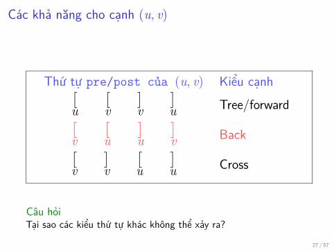
Các khả năng cho cạnh (u, v)
Thứ tự pre/post của (u, v) Kiểu cạnh[u
[v
]v
]u Tree/forward[
v[u
]u
]v Back[
v]v
[u
]u Cross
Câu hỏiTại sao các kiểu thứ tự khác không thể xảy ra?
27 / 57

Mệnh đềMột đồ thị có hướng có chu trình nếu và chỉ nếu thuật toán tìmkiếm theo chiều sâu tạo ra back edge.
Chứng minh.
P1: OSO/OVY P2: OSO/OVY QC: OSO/OVY T1: OSO
das23402 Ch03 GTBL020-Dasgupta-v10 August 10, 2006 19:18
88 3.3 Depth-first search in directed graphs
Figure 3.7 DFS on a directed graph.
AB C
F DE
G H
A
H
B C
E D
F
G
12,15
13,14
1,16
2,11
4,7
5,6
8,9
3,10
In further analyzing the directed case, it helps to have terminology for importantrelationships between nodes of a tree. A is the root of the search tree; everythingelse is its descendant. Similarly, E has descendants F , G , and H , and conversely,is an ancestor of these three nodes. The family analogy is carried further: C is theparent of D, which is its child.
For undirected graphs we distinguished between tree edges and nontree edges. Inthe directed case, there is a slightly more elaborate taxonomy:
Bac
k
Forward
Cross
Tree
A
B
C D
DFS treeTree edges are actually part of the DFS forest.
Forward edges lead from a node to a nonchild descendant inthe DFS tree.
Back edges lead to an ancestor in the DFS tree.
Cross edges lead to neither descendant nor ancestor; theytherefore lead to a node that has already been completelyexplored (that is, already postvisited).
Figure 3.7 has two forward edges, two back edges, and two cross edges. Can youspot them?
Ancestor and descendant relationships, as well as edge types, can be read off directlyfrom pre and post numbers. Because of the depth-first exploration strategy, vertexu is an ancestor of vertex v exactly in those cases where u is discovered first and
▶ Nếu (u, v) là back edge, thìu ; v → u là một chu trình.
▶ Ngược lại, giả sử đồ thị có chutrình
C = v0 → v1 → · · · → vk → v0.
Xét vi là đỉnh đầu tiên trong Cđược thăm theo DFS. Mọi đỉnhkhác trong chu trình sẽ đạt được từvi. Vậy thì vi−1 → vi là back edge.
28 / 57

Bài tập1. Hãy mô tả một thuật toán kiểm tra liệu đồ thị có hướng cho
trước có chu trình hay không.2. Hãy cài đặt thuật toán này.
29 / 57
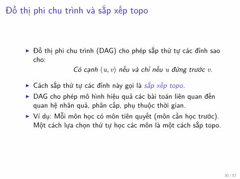
Đồ thị phi chu trình và sắp xếp topo
▶ Đồ thị phi chu trình (DAG) cho phép sắp thứ tự các đỉnh saocho:
Có cạnh (u, v) nếu và chỉ nếu u đứng trước v.
▶ Cách sắp thứ tự các đỉnh này gọi là sắp xếp topo.▶ DAG cho phép mô hình hiệu quả các bài toán liên quan đến
quan hệ nhân quả, phân cấp, phụ thuộc thời gian.▶ Ví dụ: Mỗi môn học có môn tiên quyết (môn cần học trước).
Một cách lựa chọn thứ tự học các môn là một cách sắp topo.
30 / 57

Đồ thị phi chu trình (DAG)
P1: OSO/OVY P2: OSO/OVY QC: OSO/OVY T1: OSO
das23402 Ch03 GTBL020-Dasgupta-v10 August 10, 2006 19:18
90 3.3 Depth-first search in directed graphs
Figure 3.8 A directed acyclic graph with one source, two sinks, and fourpossible linearizations.
A
B
C
D
E
F
out of bed; you have to be out of bed, but not yet dressed, to take a shower; and soon). The question then is, what is a valid order in which to perform the tasks?
Such constraints are conveniently represented by a directed graph in which eachtask is a node, and there is an edge from u to v if u is a precondition for v. In otherwords, before performing a task, all the tasks pointing to it must be completed. If thisgraph has a cycle, there is no hope: no ordering can possibly work. If on the otherhand the graph is a dag, we would like if possible to linearize (or topologically sort)it, to order the vertices one after the other in such a way that each edge goes froman earlier vertex to a later vertex, so that all precedence constraints are satisfied. InFigure 3.8, for instance, one valid ordering is B, A, D, C , E , F . (Can you spot theother three?)
What types of dags can be linearized? Simple: All of them. And once again depth-first search tells us exactly how to do it: simply perform tasks in decreasing or-der of their post numbers. After all, the only edges (u, v) in a graph for whichpost(u) <post(v) are back edges (recall the table of edge types on page 88)—andwe have seen that a dag cannot have back edges. Therefore:
Property In a dag, every edge leads to a vertex with a lower post number.
This gives us a linear-time algorithm for ordering the nodes of a dag. And, to-gether with our earlier observations, it tells us that three rather different-soundingproperties—acyclicity, linearizability, and the absence of back edges during a depth-first search—are in fact one and the same thing.
Since a dag is linearized by decreasing post numbers, the vertex with the smallestpost number comes last in this linearization, and it must be a sink—no outgoingedges. Symmetrically, the one with the highest post is a source, a node with noincoming edges.
Property Every dag has at least one source and at least one sink.
The guaranteed existence of a source suggests an alternative approach to lineariza-tion:
Phi chu trình ⇐⇒ Không có Back Edge ⇐⇒ Sắptopo
31 / 57

Bài tậpHãy đưa ra mọi cách sắp topo cho đồ thị phi chu trình sau:
P1: OSO/OVY P2: OSO/OVY QC: OSO/OVY T1: OSO
das23402 Ch03 GTBL020-Dasgupta-v10 August 10, 2006 19:18
90 3.3 Depth-first search in directed graphs
Figure 3.8 A directed acyclic graph with one source, two sinks, and fourpossible linearizations.
A
B
C
D
E
F
out of bed; you have to be out of bed, but not yet dressed, to take a shower; and soon). The question then is, what is a valid order in which to perform the tasks?
Such constraints are conveniently represented by a directed graph in which eachtask is a node, and there is an edge from u to v if u is a precondition for v. In otherwords, before performing a task, all the tasks pointing to it must be completed. If thisgraph has a cycle, there is no hope: no ordering can possibly work. If on the otherhand the graph is a dag, we would like if possible to linearize (or topologically sort)it, to order the vertices one after the other in such a way that each edge goes froman earlier vertex to a later vertex, so that all precedence constraints are satisfied. InFigure 3.8, for instance, one valid ordering is B, A, D, C , E , F . (Can you spot theother three?)
What types of dags can be linearized? Simple: All of them. And once again depth-first search tells us exactly how to do it: simply perform tasks in decreasing or-der of their post numbers. After all, the only edges (u, v) in a graph for whichpost(u) <post(v) are back edges (recall the table of edge types on page 88)—andwe have seen that a dag cannot have back edges. Therefore:
Property In a dag, every edge leads to a vertex with a lower post number.
This gives us a linear-time algorithm for ordering the nodes of a dag. And, to-gether with our earlier observations, it tells us that three rather different-soundingproperties—acyclicity, linearizability, and the absence of back edges during a depth-first search—are in fact one and the same thing.
Since a dag is linearized by decreasing post numbers, the vertex with the smallestpost number comes last in this linearization, and it must be a sink—no outgoingedges. Symmetrically, the one with the highest post is a source, a node with noincoming edges.
Property Every dag has at least one source and at least one sink.
The guaranteed existence of a source suggests an alternative approach to lineariza-tion:
32 / 57

Tính chất của DAG
Mệnh đềTrong DAG, nếu (u, v) ∈ E thì post(u) > post(v).
Vậy thì các đỉnh của DAG có thể sắp topo theo thứ tự giảm dầncủa post.
33 / 57

Bài tậpXét một DAG có pre và post như dưới đây. Hãy đưa ra một thứtự topo cho các đỉnh.
1
0
3
25
47
6
9
8
0 : [1, 16]1 : [17, 18]2 : [2, 9]3 : [3, 8]4 : [19, 20]5 : [4, 7]6 : [11, 14]7 : [10, 15]8 : [12, 13]9 : [5, 6]
34 / 57
Bài tập1. Hãy mô tả một thuật toán sắp Topo cho một DAG.2. Hãy cài đặt thuật toán này.
35 / 57

Đỉnh nguồn và đỉnh hút
P1: OSO/OVY P2: OSO/OVY QC: OSO/OVY T1: OSO
das23402 Ch03 GTBL020-Dasgupta-v10 August 10, 2006 19:18
90 3.3 Depth-first search in directed graphs
Figure 3.8 A directed acyclic graph with one source, two sinks, and fourpossible linearizations.
A
B
C
D
E
F
out of bed; you have to be out of bed, but not yet dressed, to take a shower; and soon). The question then is, what is a valid order in which to perform the tasks?
Such constraints are conveniently represented by a directed graph in which eachtask is a node, and there is an edge from u to v if u is a precondition for v. In otherwords, before performing a task, all the tasks pointing to it must be completed. If thisgraph has a cycle, there is no hope: no ordering can possibly work. If on the otherhand the graph is a dag, we would like if possible to linearize (or topologically sort)it, to order the vertices one after the other in such a way that each edge goes froman earlier vertex to a later vertex, so that all precedence constraints are satisfied. InFigure 3.8, for instance, one valid ordering is B, A, D, C , E , F . (Can you spot theother three?)
What types of dags can be linearized? Simple: All of them. And once again depth-first search tells us exactly how to do it: simply perform tasks in decreasing or-der of their post numbers. After all, the only edges (u, v) in a graph for whichpost(u) <post(v) are back edges (recall the table of edge types on page 88)—andwe have seen that a dag cannot have back edges. Therefore:
Property In a dag, every edge leads to a vertex with a lower post number.
This gives us a linear-time algorithm for ordering the nodes of a dag. And, to-gether with our earlier observations, it tells us that three rather different-soundingproperties—acyclicity, linearizability, and the absence of back edges during a depth-first search—are in fact one and the same thing.
Since a dag is linearized by decreasing post numbers, the vertex with the smallestpost number comes last in this linearization, and it must be a sink—no outgoingedges. Symmetrically, the one with the highest post is a source, a node with noincoming edges.
Property Every dag has at least one source and at least one sink.
The guaranteed existence of a source suggests an alternative approach to lineariza-tion:
Trong đồ thị có hướng,▶ Đỉnh nguồn (source) là đỉnh không có cạnh đi vào.▶ Đỉnh hút (sink) là đỉnh không có cạnh đi ra.
36 / 57

Tính chất của DAG
Mệnh đề (Nhắc lại)Trong DAG, nếu (u, v) ∈ E thì post(u) > post(v).
Vậy thì các đỉnh của DAG có thể sắp topo theo thứ tự giảm dầncủa post.
Và khi đó, đỉnh có post nhỏ nhất sẽ nằm cuối danh sách, và vậythì nó phải là đỉnh hút.
Tương tự, đỉnh có post lớn nhất là đỉnh nguồn.
37 / 57

Mệnh đềMọi DAG đều có ít nhất một đỉnh nguồn và ít nhất một đỉnh hút.
Bài tậpHãy chứng minh mệnh đề trên.
38 / 57

Thuật toán sắp topo (thứ 2)
▶ Tìm một đỉnh nguồn, ghi ra nó, và xóa nó khỏi đồ thị.▶ Lặp lại cho đến khi đồ thị trở thành rỗng.
39 / 57
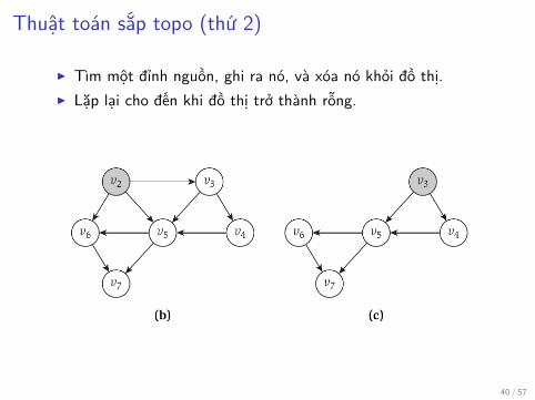
Thuật toán sắp topo (thứ 2)
▶ Tìm một đỉnh nguồn, ghi ra nó, và xóa nó khỏi đồ thị.▶ Lặp lại cho đến khi đồ thị trở thành rỗng.
40 / 57
Thuật toán sắp topo (thứ 2)
▶ Tìm một đỉnh nguồn, ghi ra nó, và xóa nó khỏi đồ thị.▶ Lặp lại cho đến khi đồ thị trở thành rỗng.
41 / 57

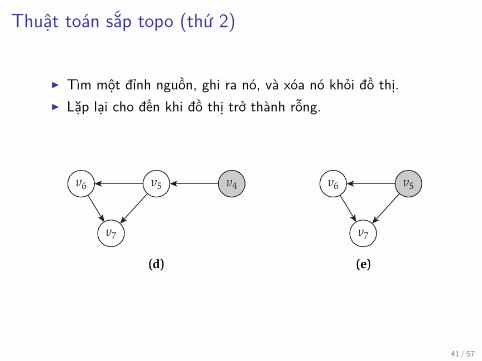
Thuật toán sắp topo (thứ 2)
▶ Tìm một đỉnh nguồn, ghi ra nó, và xóa nó khỏi đồ thị.▶ Lặp lại cho đến khi đồ thị trở thành rỗng.
42 / 57

Bài tậpChạy thuật toán sắp topo trên đồ thị sau:
1. Chỉ ra số pre và post của mỗi đỉnh.2. Tìm các đỉnh nguồn và đỉnh hút của đồ thị.3. Tìm thứ tự topo theo thuật toán.4. Đồ thị này có bao nhiêu thứ tự topo?
43 / 57

Câu hỏi
▶ Tại sao thuật toán trước cho một thứ tự topo?▶ Nếu đồ thị có chu trình thì thuật toán gặp vấn gì?▶ Làm thế nào để cài đặt thuật toán này trong thời gian tuyến
tính?
44 / 57

Nội dung
Biểu diễn đồ thị
Tìm kiếm theo chiều sâu trên đồ thị vô hướng
Tìm kiếm theo chiều sâu trên đồ thị có hướng
Thành phần liên thông mạnh

Thành phần liên thông mạnh
Định nghĩaHai đỉnh u và v của một đồ thị có hướng là liên thông nếu có mộtđường đi từ u tới v và một đường đi từ v tới u.
Quan hệ này phân hoạch tập đỉnh V thành các tập rời nhau và tagọi các tập rời nhau này là các thành phần liên thông mạnh.
46 / 57

Thành phần liên thông mạnh
P1: OSO/OVY P2: OSO/OVY QC: OSO/OVY T1: OSO
das23402 Ch03 GTBL020-Dasgupta-v10 August 10, 2006 19:18
Chapter 3 Algorithms 91
Find a source, output it, and delete it from the graph.
Repeat until the graph is empty.
Can you see why this generates a valid linearization for any dag? What happens ifthe graph has cycles? And, how can this algorithm be implemented in linear time?(Exercise 3.14.)
3.4 Strongly connected components3.4.1 Defining connectivity for directed graphsConnectivity in undirected graphs is pretty straightforward: a graph that is not con-nected can be decomposed in a natural and obvious manner into several connectedcomponents (Figure 3.6 is a case in point). As we saw in Section 3.2.3, depth-firstsearch does this handily, with each restart marking a new connected component.
In directed graphs, connectivity is more subtle. In some primitive sense, the directedgraph of Figure 3.9(a) is “connected”—it can’t be “pulled apart,” so to speak, with-out breaking edges. But this notion is hardly interesting or informative. The graphcannot be considered connected, because for instance there is no path from Gto B or from F to A. The right way to define connectivity for directed graphs isthis:
Two nodes u and v of a directed graph are connected if there is a path from u tov and a path from v to u.
Figure 3.9 (a) A directed graph and its strongly connected components. (b) Themeta-graph.
(a)A
D E
C
F
B
HG
K
L
JI
(b)
A B,E C,F
DJ,K,LG,H,I
Hình: (a) Đồ thị có hướng và các thành phần liên thông mạnh. (b) Cácthành phần liên thông mạnh tạo thành một DAG
47 / 57

Các thành phần liên thông mạnh trong đồ thị
Mệnh đềMọi đồ thị có hướng đều là một DAG của các thành phần liênthông mạnh.Vì nếu có chu trình đi qua một số thành phần liên thông mạnh thìcác thành phần này phải được gộp chung lại thành một thànhphần liên thông mạnh.
48 / 57

Một số tính chất
Mệnh đềNếu thủ tục con explore bắtđầu từ một đỉnh u, thì nó sẽkết thúc khi mọi đỉnh có thểđến được từ u đã được thăm.
49 / 57

Một số tính chất
Nếu ta gọi explore từ một đỉnhthuộc một thành phần liên thôngmạnh hút, vậy thì ta sẽ nhậnđược đúng thành phần này.
50 / 57
Câu hỏi
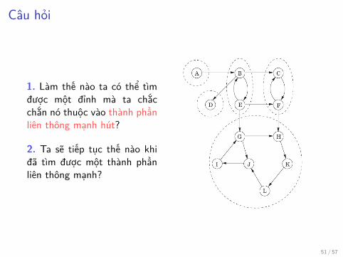
1. Làm thế nào ta có thể tìmđược một đỉnh mà ta chắcchắn nó thuộc vào thành phầnliên thông mạnh hút?
2. Ta sẽ tiếp tục thế nào khiđã tìm được một thành phầnliên thông mạnh?
51 / 57

Câu hỏi 1Làm thế nào ta có thể tìm được một đỉnh mà ta chắc chắn nóthuộc vào thành phần liên thông mạnh hút?Xét GR là đồ thị ngược của G, tức là đồ thị GR đạt được từ Gbằng cách đảo hướng các cạnh.
Thành phần liên thông mạnh của G cũng là của GR. Tại sao?
Và thành phần liên thông mạnh hút trong G sẽ là thành phần liênthông mạnh nguồn trong GR.Mệnh đềĐỉnh có số post lớn nhất theo DFS phải thuộc một thành phầnliên thông mạnh nguồn.
52 / 57

Hình: Đồ thị G Hình: Đồ thị ngược GR của G
53 / 57

Câu hỏi 2Ta sẽ tiếp tục thế nào khi đã tìm được một thành phần liên thôngmạnh?
Mệnh đềNếu C và D là các thành phần liên thông mạnh, và có một cạnhtừ một đỉnh trong C tới một đỉnh trong D, vậy thì số post lớnnhất trong C phải lớn hơn số post lớn nhất trong D.
Khi ta tìm thấy một thành phần liên thông mạnh và xóa nó khỏiđồ thị G, vậy thì đỉnh với số post lớn nhất trong các đỉnh còn lạisẽ thuộc vào thành phần liên thông mạnh hút của đồ thị còn lạicủa G.
54 / 57

Thuật toán tìm thành phần liên thông mạnh1. Chạy DFS trên đồ thị ngược GR của G.2. Chạy thuật toán tìm thành phần liên thông (tương tự như của
đồ thị vô hướng) trên đồ thị có hướng G; và trong khi chạyDFS, xử lý các đỉnh theo thức tự giảm dần theo số post củamỗi đỉnh.
55 / 57

Bài tậpChạy thuật toán tìm thành phần liên thông mạnh trên đồ thị sau(theo thứ tự từ điển).
56 / 57

Bài tậpChạy thuật toán tìm thành phần liên thông mạnh trên đồ thị sau(theo thứ tự từ điển).
57 / 57