Title Some Mathematical Considerations on Parent-OffspringConflict Phenomenon(Mathematical Topics in Biology)

Author(s) SENO, Hiromi; TOKUDA, Hiroki

Citation 数理解析研究所講究録 (1994), 870: 227-238

Issue Date 1994-05

URL http://hdl.handle.net/2433/84006

Right

Type Departmental Bulletin Paper

Textversion publisher

Kyoto University

227

Some Mathematical Considerationson Parent-Offspring Conflict Phenomenon

Hiromi SENO and Hiroki TOKUDADepartment of Mathematics, Faculty of Science, Hiroshima University

子の独立時期についての親子間衝突に関する数理モデル解析

瀬野裕美・徳田博樹広島大学理学部

A stochastic dynamic programming model for parent-offspring confict is analyzed and discussed. It is discussedhow the confiict is resolved and how the ultilllate off-spring’s independence age is determined between parentand offspring. Results by the mathematical model in-dicates such possibility that the observed behaviour ofparental care may ch ange depending on the parent’s age.This is because the compromise conclusion of the parent-offspring conflict depends on the parent’s age, that isessentially, on the parent’s expected future reproductivevalue. Moreover, it is shown that the observed parent-offspring confbct possibly depends on the parent’s age,too.

INTRODUCTION

In behavioural ecology, many researchers havebeen interested in and have discussed the parent-offspring conflict phenomenon: offspring wants tobecome independent of parent and to feed by it-self after an age $t_{o},$ $w1_{1}ile$ parent of its age $a$ wantsto stop feeding after an offspring’s age $t_{p}(a)$ . Thecritical day $t_{p}(a)$ from the parent’s viewpoint isassumed to depend on the parent’s age $a$ . When$t_{o}$ and $t_{p}(a)$ do not coincide with each other, aconflict takes place between parent and offspring.There are possibly two different types of such con-flict: $t_{o}^{l}<t_{p}(a);t_{o}>t_{p}^{l}(a)$ . Under the conflict inthe case when $t_{o}<t_{p}(a)$ , offspring wants to be-come independent of parent, while parent wantsto feed offspring. On the other hand, in the casewhen $t_{o}>t_{p}(a)$ , offspring wants to be fed, while

parent wants to stop feeding. Only when $t_{o}=$

$t_{p}(a)$ , any conflict doesn’t take place. However,since $t_{o}$ does not depend on the parent’s age $a$ ,whereas $t_{p}(a)$ does, the conflict between parentand offspring is observable very much.In this work, we analyze a stochastic dynamic pro-gramming model which corresponds to the modelconstructed by Clark and Ydenberg (1990). Inour model, differently from their model, parent isassumed to have a finite reproducible age-span,so that its future reproductive value is explicitlyvariable depending on the parent’s age. A spe-cific growth function and a specific terminal fitnessfunction are introduced. Analyzing the model, wediscuss the characteristics of the optimal criticalages $t_{o}$ and $t_{p}(a)$ , and it is shown that possibly ex-istent conflict is only the type that $t_{o}>t_{p}(a)$ , in-dependently of the parent’s age and the other pa-rameters characterizing the relation between par-ent and offspring. Further, we discuss how theconflict is resolved and how tbe ultimate indepen-dence age is determined between parent and off-spring.

MODEL

Parent’s and Offsprrng’s Ages

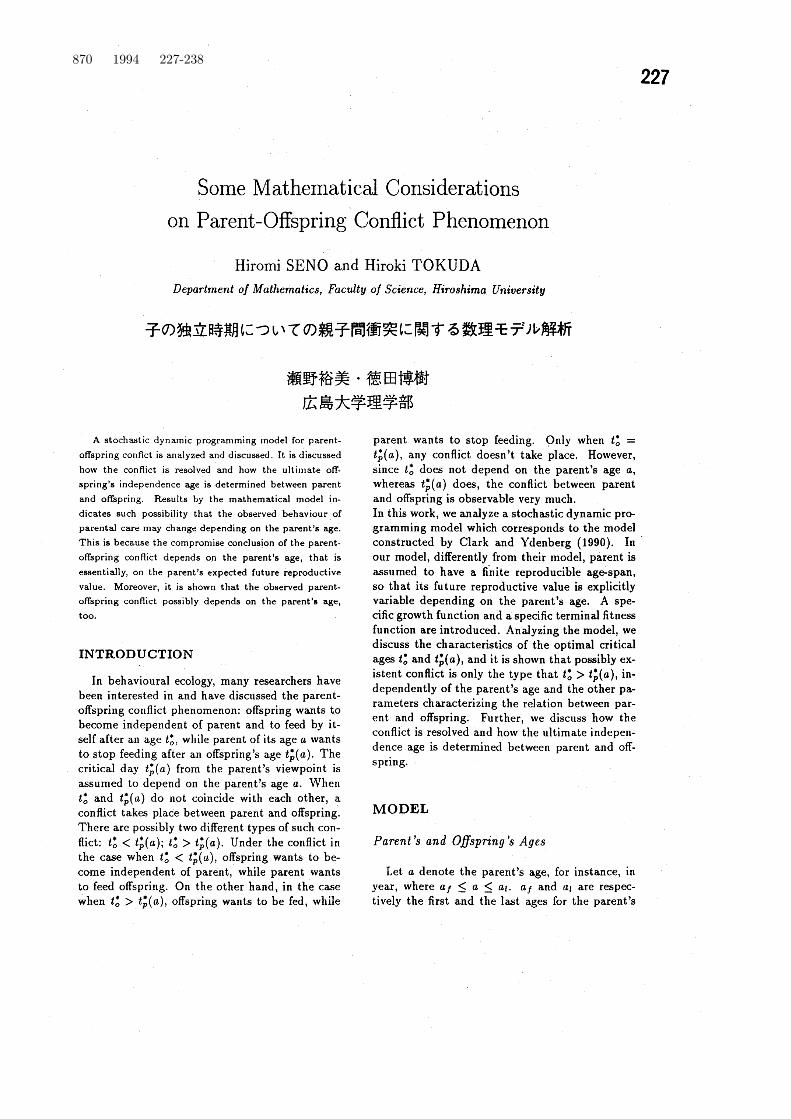
Let $a$ denote the parent’s age, for instance, inyear, where $a_{f}\leq a\leq a_{1}$ . $a_{f}$ and $a_{1}$ are respec-tively the first and the last ages for the parent’s

数理解析研究所講究録第 870巻 1994年 227-238

228parents reproduCible ages

$\underline{a_{f}}$$\underline{\varphi+1}$ – $—-,’ \backslash -\underline{a}\sigma_{\nu}\bigcap_{\backslash }\backslash ----$

$\underline{a_{t}}$

bneang$”’$

’

$\sim$

$\infty aen$ $\sim_{s}$

$\vdash’’+^{\prime d\text{下_{}-}sa\underline{fter0\Uparrow}\underline{sbi}rt\text{加^{}\backslash }\backslash }\infty’\div-\infty^{\backslash }\{""\prime y_{-}sp\dot{n}n_{9_{-}’\backslash }\backslash \backslash \backslash \backslash$

12 $t_{l}$ r-l $T$

$-hnnt*\prime c_{n}\text{\’{e}} n(o_{f},\sigma)arrow 2^{o\kappa_{\epsilon m\eta\dot{\}}}j_{nm_{\sigma_{r}^{n}}\infty_{\sigma_{o})}}$

(

Fig. 1. Modelling the parent-offspring relauon.

reproduction. Hence, the reproducible age-spanfor every parent is given by $a\iota-a_{f}+1$ . The off-spring’s age in day during a breeding season isdenoted by $t$ , where $1\leq t\leq T$ . $T$ is the length inday of breeding season (see Fig. 1).

Offsp7ring $s$ Growth

We use the following specific growth functionfor offspring:

$Y(t+1)=\{Y(t)+Y(t)+k_{t=t,t_{S}+1^{s},..,T-1}fort^{1}=1_{s}2,\ldots,t-.1r\circ r^{k_{2}}(I)$

$Y(1)=Y_{1}$ , (2)

that is,

$Y(t)=\{\begin{array}{l}k_{1}(t-1)+Y_{1}k_{2}(t\frac{}{f}t_{S})+k_{s^{1}}(t_{\delta}-1)+Y_{1}r_{ort=1,2_{\prime}}ort=t+1_{\prime}t^{t_{s^{S}}}+2,\ldots,T\end{array}$ (3)

where $Y(t)$ is the offspring’s weight at the begin-ning of day $t$ , and $Y_{1}$ is the offspring’s weight at itsbirth. $t_{s}$ is the offspring’s age when parent stops

. feeding and offspring becomes independent. $k_{1}$ isa positive constant which means the offspring’sdaily growth rate with the parent’s feeding, while$k_{2}$ is a positive constant which means the inde-pendent offspring’s daily growth rate (see Fig. 2).

Now, consider the offspring’s weight $Y(T;t_{s})$ atthe beginning of thelast day $T$ of the breeding sea-son, under the condition that offspring becomesindependent at day $t_{s}$ . From (3), $Y(T;t_{s})$ is ex-pressed as follows:

$Y(T, t_{\theta})=k_{2}(T-t_{S})+k_{1}(t_{S}-1)+Y_{1}$ . (4)

Offspring’s Fitness

We define the daily survival probability $\sigma_{n}$ foroffspring fed by parent, the daily survival proba-bility $\sigma_{o}$ for offspring independent of parent, thedaily survival probability $\sigma_{f}$ for parent feeding off-spring, and the daily survival probability $\sigma_{p}$ forparent not feeding offspring (see Fig. 1). AsYdenberg (1989) showed in general for alcids, itis naturally assumed that $\sigma_{o}<\sigma_{n}$ and $\sigma_{f}<\sigma_{p}$ .The following events significant to determine theoffspring’s fitness are assumed on each day: (i)If parent survives and feeds offspring with prob-ability $\sigma_{f}$ , offspring grows following to (3) withits survival probability $\sigma_{n}$ ; (ii) $|If$ parent dies with

probability $1-\sigma_{f}$ , offspring becomes independentto grow following to (3) with its survival probabil-ity $\sigma_{o}$ ; (iii) If parent stops feeding offspring withits survival probability $\sigma_{p}$ , offspring becomes inde-pendent to grow following to (3) with its survivalprobability $\sigma_{o}$ .

Consider such probability $\phi(1^{\prime’}(T;t_{\dot{\theta}}))$ that off-spring $wit1_{1}$ weight $Y(T;t_{s})$ at the end of thebreeding season will survive after the breeding sea-son and reach the reproducible age to reproducethe next generation. The probability $\phi(Y(T;t_{s}))$

is called the terminal fitness function for offspring,and given as follows:

$\phi(1’(T;t_{s}))=\{$ $\gamma(YT\cdot t)0oth’erwise^{y}!t_{S})>y_{C};(5)$

where $\gamma$ is a positive constant translating the ad-vantage of weight gain $Y(T;t_{s})-y_{C}$ to the prob-ability $\phi(Y(T;t_{S}))$ . $y_{C}$ is the offspring’s minimumbody weight at the end of the breeding season,sufficient to survive after the breeding season andreach its reproducible age to reproduce the nextgeneration (see Fig. 3).

Conventionally, we define the critical day $t_{c}$

such that $Y(T;t_{c})=y_{c}$ , which is given by

$t_{c} \equiv\frac{y_{C}-Y_{1}+k_{1}-k_{2}T}{k_{1}-k_{2}}$ . (6)

Used the notation $t_{c}$ , the probability $\phi(Y(T;t_{s}))$

can be expressed in the following way:When $k_{1}>k_{2}$ ,

$\phi(Y(T;t_{s}))=\{\begin{array}{l}\gamma(k_{1}-k_{2})(t_{s}ift_{S}>^{-}t^{t_{c^{c}}.,)}0otherwise\end{array}$ (7)

When $k_{1}<k_{2}$ ,

(8)$\phi(Y(\mathcal{T};t_{\delta}))=\{\begin{array}{l}\gamma(k_{2}-k_{1})(t_{c}if\ell_{S}<^{-}\ell^{\iota_{c^{s}}.)}0otherwise\end{array}$

Eventually, it is assumed that $1<t_{c}<T$ . In thecase when $k_{1}>k_{2}$ , if the offspring’s independenceday $t_{s}$ is earlier than the critical day $[t_{c}]+1$ givenby (6), the offspring’s weight $Y(T;t,)$ at the endof the breeding season is below $y_{c}$ so that the ter-minal fitness function $\phi(Y(T;t_{s})$ is zero (Fig. 3).In contrast, in the case when $k_{1}<k_{2}$ , if the off-spring’s independence day $t_{s}$ is later than $[t_{c}]$ , theterminal fitness function $\phi(Y(T;t_{s})$ is zero.

Now, we consider the offspring’s fitness $F_{o}(t_{s})$

defined as such probability that offspring can sur-vive through and after the breeding season andreach its reproducible age to reproduce the next

$k_{1}>k_{2}$ $k_{1}<k_{2}$229

Fig. 2. Offspring’s growth function $Y(t)$ for two cases: when $k_{1}>k?\sim$ and thegrowth rate is larger under the parent’s feeding than after the offspring’sindependence; when $k_{1}<k_{2}$ and the growth rate has the inverse nature.Offspring has the weight $Y_{1}$ at its birth. lf offspnng becomes independentof parent on the day $t_{S}$. it reaches the weight $Y(T;t_{s})$ at the end of thebreeding season.

$k_{1}>k_{2}$ $k_{1}<k_{2}$

Fig. 3. Terrmnal fitness function $\phi(Y(T;t))$ given by (5). There exists such acnuca! day for the offspnng’s independence that the terminal fitnessfunction $\phi(Y(T;t))$ is zero tor any independence day $t$ before or after thecntical day.

230

generation, under the condition that it becomesindependent on day $t_{S}$ of the breeding season. Ifoffspring becomes independent on the first day,that is, $t_{s}=1$ , it survives through the breedingseason with probability $\sigma_{o}^{T}$ . Growing up with (3),the offspring’s weight reaches $Y(T;1)$ at the lastday $T$ of the breeding season, which means that,after the breeding season, offspring gets the prob-ability $\phi(Y(T;1))$ to survive and reach its repro-ducible age. Hence, the offspring’s fitness $F_{o}(1)$ isgiven by

$F_{o}(1)=\sigma_{o}^{T}\phi(Y(T;1))$. (9)

In the case when $t_{s}=2$ , two cases arise to beconsidered. The first case is that, if parent dies onthe first day with probability $1-\sigma_{f}$ , offspring is

i糖鍛鰯響鞭\not\in n漉難窺難$pt$嚇 hernepet撫ability $\sigma_{o}^{T}$ . Therefore, the fitness in this case isgiven by $F_{o}(1)$ with probability $1-\sigma_{f}$ . The second

詳諸認織雅 r認撒響 fd,講 r離播and survives for one day with probability $\sigma_{n}$ . For$o^{s}n\overline{\overline{d}}d^{\sim}t_{therest\circ fthebreedingseason^{ri_{W1}survives}}^{0ffs}Tl9throug^{a}f_{en,theindependentoffspng_{thproba-}}^{ri\iota\iota gbecomesindependentonthe\sec-}$

bilty $\sigma_{O}^{T-1}$ . The offspring‘s weight reaches $Y(T;2)$on day $T$ , which means that, after the breedingseason, offspring gets the probability $\phi(Y(T;2))$

to survive and reach its reproducible age. Lastly,the offsping’s fitness $F_{o}(2)$ is given by

$F_{O}(2)=$ ( $1$ –a$f$ ) $\sigma_{O}^{T}\phi(Y(T;1))$

(10)

$+\sigma_{f}\sigma_{n}\sigma_{o}^{T-1}\phi(Y(’\Gamma;^{o}\sim))$ .

In the case when $t_{s}=3$ , three cases arise. Thefirst case is that parent dies on the first day withprobability $1-\sigma_{f}$ . The second case is that parentsurvives on the first day with probability $\sigma_{f}$ anddies on the second day with probability $1-\sigma_{f}$ . Inthis case from the second day, offspring becomes$independ_{en}t$ and survives through the rest of the

$Caseisb\circ thofbreedin_{t}fi_{th^{a}e}^{se_{t}asonwithprobabi1ity_{feedsoffs}}\not\in arentsurvivesandf_{proba-}^{ringon}$

$T-1$ . The third

bility $\sigma_{f}^{2}$ . In this case, offspring survives for twodays with probability $\sigma_{n}^{2}$ . For $t_{s}=3$ , offspringbecomes independent on the third day. The mde-pendent offspring survives through the rest of thebreeding season with probability $\sigma_{o}^{T-2}$ . Lastly, theoffspring’s fitness $F_{o}(3)$ is given by

$F_{o}(3)=(1-\sigma_{f})\sigma_{o}^{T}\phi(Y(T;1))$

$+\sigma_{f}(1-\sigma_{f})\sigma_{n}\sigma_{o}^{T-1}\phi(Y(T;2))$(11)

$+\sigma_{f}^{2}\sigma_{n}^{2}a_{o}^{T-2}\phi(Y(T;3))$ .

For the case when $t_{s}=4,5,$ $\ldots,$$T,$ $F_{o}(t_{s})$ is given

in the same way.Consequently, except for the case when $t_{s}=$

$1,$ $F_{o}(t_{s})$ is expressed in general as follows:

$F_{O} \langle l,)=\sum_{j=1}^{t_{*}-1}\sigma_{f}^{j-1}\langle 1-\sigma_{j})\sigma_{\mathfrak{n}}^{j-1}\sigma_{O}^{T-j+1}\phi(Y^{-}(T:j))$

$+\sigma_{j}^{1-1}\sigma_{n^{l}}^{l-1}\sigma_{o}^{T-t_{9}+1}\phi(Y(T;\ell_{i}))$ .

(12)

Parent’s Survival Probability

In this section, We consider the parent’s sur-vival probability $F_{p}(t_{s})$ , which is defined assuch probability that parent survives through thebreeding season under the condition that it stopsfeeding on day $t_{s}$ in the breeding season. Now, $\sigma_{w}$

is defined as such probability that parent survivesthrough the interval period between two sequentbreeding seasons and reaches the next breedingseason.

If parent never feeds offspring on any daythrough the breeding season, that is, if $t_{S}=1$ ,parent survives through the breeding season withprobability $\sigma_{p}^{T}$ . Then, parent can reach the nextbreeding season with probability $\sigma_{w}$ . Hence, theparent’s survival probability $F_{p}(1)$ is given by

$F_{P}(1)=\sigma_{p}^{T}\sigma_{w}$ . (13)

If parent feeds offspring on the first day andstops feeding on the second day, that is, if $t_{s}=2$ ,parent survives on the first day with probability$\sigma_{f}$ and through the rest of the breeding seasonwith probability $\sigma_{p}^{T-1}$ . Hence, the parent’s sur-vival probability $F_{p}(2)$ is given by

$F_{p}(2)=a_{f}a_{p}^{T-1}\sigma_{w}$ . (14)

In the case when $t_{s}=3$ , two cases arise to beconsidered. The first case is that parent feeds off-spring on the first day with its survival probability$\sigma_{f}$ , while offspring dies on the first day with prob-ability $1-\sigma_{n}$ . Then, parent survives through therest of the breeding season with probability $\sigma_{p}^{T-1}$ .The second case is that parent feeds offspring onthe first day with its survival probability $\sigma_{f}$ , whileoffspring survives on the second day with its sur-vival probability $\sigma_{n}$ . Parent feeds offspring alsoon the second day with its survival probability$\sigma_{f}$ . For $t_{s}=3$ , parent stops feeding on the thirdday. Then, parent survives through the rest of thebreeding season with probability $\sigma_{p}^{T-2}$ . Lastly, theparent’s survival probability $F_{p}(3)$ is given by

231

$F_{p}(3)=\{(1-\sigma_{n})a_{f}\sigma_{p}^{T-}+a_{n}a_{f}^{2}\sigma_{p}^{T-2}\}\sigma_{w}.(15)$

For the case when $t_{S}=4,5,$$\ldots,$

$T,$ $F_{p}(t_{s})$ is givenin the same $wav$.

Consequently, except for the case when $t_{s}=1$

or $t_{s}=2,$ $F_{p}(t_{s})$ is expressed in general as follows:

$F_{p}(t_{s})$ $=a_{w} \sum_{j=1}^{t,-2}\sigma_{n}^{j-1}(1-a_{n})\sigma_{f}^{j}a_{p}^{T-j}$

(16)

$+a_{w}\sigma_{n}^{t.-2}\sigma_{f}^{t.-1}\sigma_{p}^{T-\iota.+1}$ .

reproductive value $R(a_{1}-1)$ for the age $a\iota-1$ isdetermined by

$R(a_{l}-I)$ $=$ $\sigma_{w}J(t_{p}(a_{\iota});R(a_{\iota}))$

$=$ $a_{w}F_{O}(i_{p}(a_{\iota}))$ , (19)

and, further, in general, the value $R(a_{l}-i)(i=$$1,2,$

$\ldots,$$a\iota$ –a$’$ ) for the age $a\iota-i$ is given by the

following backward recurrence equation:

$R(a_{\iota}-i)=\sigma_{w}J(t_{p}(a_{\iota}-i+1);R(a_{l}-i+1)).(20)$

MODEL

Parent’s Fitness

Consider the parent’s fitness at its age $a$ , underthe condition that it stops feeding on day $t_{s}$ of thebreeding season. The parent’s fitness $J(t_{s}; R(a))$

is defined by the parent’s survival probability$F_{p}(t_{s})$ , its offspring’s fitness $F_{o}(t_{s})$ , and the par-ent’s expected future reproductive value $R(a)$ atthe last day of the breeding season at the parent’sage $a$ , which satisfies the following:

$R(a)=a_{w}J(t_{S}; R(a+1))$(17)

$(a=a_{f}, a_{f}+1, \ldots, a_{\iota}-1)^{-}$

$J(t_{s} ; R(a+1))$ means the parent’s fitness at itsage $a+1$ . Since $\sigma_{w}$ means the probability thatparent survives between the end of the breedingseason at its age $a$ and the beginning of the nextbreeding season at its age $a+1$ , the righthand sideof (17) means the expected future reproductivevalue. Remark that $R(a)$ should be monotonicallydecreasing in terms of the age $a$ , and $R(a\iota)=0$

because $a_{l}$ is the last age for the parent’s repro-duction.

As in Clark and Ydenberg (1990), $J(t_{s}; R(a))$

is given in this paper as follows:

$J(t_{S} ; R(a))=F_{O}(t_{S})+R(a)F_{p}(t_{S})$ . (18)

From (17) and (18), we can obtain the backwardrecurrence equation to determine the expected fu-ture reproductive value $R(a)$ for every age $a$ . Itis assumed that, since the expected future repro-ductive value $R(a)$ is considered only for parent todetermine its behaviour $t_{p}(a)$ from its viewpoint,it has no relation with $t_{o}$ from the offspring’s view-point. Thus, since $R(a_{\iota})=0$ , the expected future

ANALYSIS

The Optimal Offspring $s$ Independence AgeFrom The Offspring’s Viewpoint

The $opt_{!}md$ offspring’s independence age $t_{o}$

from offspring’s $viewp_{01}nt$ is defined as the dayto maximize the offspring’s fitness $F_{o}(t_{s})$ in thebreeding season. Therefore, by analyzing $F_{o}(t_{s})$

given by (9) and (12) (as for the way of analysis,see Appendix A), $t_{o}$ can be obtained as follows(Fig. 4):

When $k_{1}>k_{2}$ ,

$\ell_{O}=T$ . (21)

When $k_{1}<k_{2}$ ,

$t_{o}=\{\begin{array}{l}n1ift<\nu+if\nu^{c}+n<t_{c\leq}^{2}\nu+n+1(n=2,3,\ldots\prime T-1)\end{array}$ (22)

where

$\nu\equiv\frac{1}{\sigma_{n}/\sigma_{O}-1}$ . (23)

Since $\sigma_{n}>\sigma_{o}$ from the assumption, $0<\nu<\infty$ .For convenience, we will hereafter use the notation$\nu$ .

As seen in Fig. 4, those conditions for $t_{o}$ in thecase when $k_{1}<k_{2}$ , given by (22), are complemen-tary each $otl\iota er$ , and the possibly maximal $F_{o}(t_{s})$

is $T-1$ in the case.

The Optimal Offspring’s Independence AgeFrom Parent’s Viewpoint

The optimal offspring’s independence age $t_{p}^{l}(a)$

from the parent’s viewpoint is defined as the off-spring’s age $t_{s}|$ to maximize the parent’s fitness$J(t_{s};R(a))$ . By analyzing $J(t_{s}; R(a))$ given by ,

232

Fig. 4. In the case when $k_{1}<k_{2}$ , the optimal offspnng’s independence age $t_{o^{*}}$

from the offspnng’s viewpoint on the parameter space $(V, t_{c})$ . For $1<t_{c}<$

$T,$ $t_{o}^{*}<T$.

Fig. 5. In the case when $k_{1}>k_{2}$ , the parameter space $(p. K(n))$ is categorizedinto $I_{1}-I_{7}$ , depending on the type ot the division of the parameter space$(v, t_{c})$ in terms of the value $0\dot{f}t_{p}^{*}(\iota)$ .

$I_{1}$ $I_{2}$

$I_{3}$ $L$

Fig. 6. $\ln$ the case when $k_{1}>k_{2}$ , the optimal oftspring $s$ independence ,Igc$t_{p}^{*}(a)$ from the parent’s viewpoint on the $pu\phi met_{C^{\backslash }}r$ space $(v, t\cdot)$ for theparameter sets $I_{1}-I_{4}$ of the parameter space $(p, K(\iota))$ .

Fig. 7. In the case when $k_{1}>k_{2}$, the optimal offspring’s independence age$t_{p^{*}}(a)$ from the parent’s viewpoint on the parameter space $(v, t_{c})$ tor theparameter sets $I_{5}-I_{7}$ of the parameter space $(p. K(l))$ .

233

Fig. 8. In the case when $k_{1}<k_{2}$ , the parameter space $(p, \mathfrak{l}K(a)1)$ is categonzedinto $C0$. $C_{dt}$ , and $C_{2}\sim Cr-2$, depending on the type of the division ofthe parameter space $(v, t_{c})$ in terms of the value of $t_{p^{*}}(a)$.

Fig. 9. In the case when $k_{l}<k_{2}$ , the optimal offspnng’s independence age$t_{P^{*}}(a)$ from the parent’s viewpoint on the parameter space $(v, t_{c})$ for theparameter sets, $C_{0},$ $C_{all}$ , and $C_{n}(n=2,3, \ldots, T-2)$ of the parameter space( $p$ , I$K(a)I$ ).

234

(18), $t_{p}(a)$ can be obtained for the parent’s age$a$ , when $R(a)>0$ , that is, when a $f\leq a\leq a_{\iota}-1$ ,as follows:

When $k_{1}>k_{2}$ ,

$t_{p}(a)=\{Tlni^{i\leq_{+_{\ell}^{t<}}^{(\nu_{C}\cdot a\rangle_{(\nu\cdot.\alpha_{\circ)}}}}i_{ T\leq_{T\frac{9}{h}}}i^{ft>_{(n_{l}=}}orilt<^{2}orii\ell<_{\mathfrak{n}+_{2^{l_{\prime}}}^{n^{l_{\frac{\{}{ct_{3}}}}}}^{n}n_{an_{d^{c^{l}}h_{C}\nu.a.)\leq t_{C}<h_{n}\langle\nu.\alpha)}}^{c}an_{-}^{d_{C}h^{g}\nu\cdot...a_{\nu}).\leq.l_{C}<.g_{\mathfrak{n}}\{\nu\cdot..a\rangle}and\ell c<r^{<_{l}\tau^{T_{)}-l)}}an^{-}d\ell<\tau^{l}t^{n}’$ (24)

When $k_{1}<k_{2}$ ,

$t_{p}(a)=\{n1i^{ft<h(\nu.\cdot a)}i_{fh^{c_{n}}(\nu\cdot.a)<t_{c}..\leq h_{n+}(n=^{1}2,3,.,T-1^{1})^{(\nu\cdot.a)}}$ (25)

where

$g_{n}( \nu;a)\equiv n+\frac{\rho^{T-n+2}\nu}{K(a)\nu+1}$ (26)

$h_{\hslash}( \nu;a)\equiv n+(1-\frac{\rho^{T-n+2}}{K(a)})\nu$ (27)

$\rho\equiv\frac{\sigma_{p}}{\sigma_{O}}$ (28)

$K(a) \equiv\frac{\gamma(k_{1}-k_{2})\sigma_{P}/\sigma_{w}}{R(a)\sigma_{p}/\sigma_{f}-1}$ . (29)

Note that those conditions for $t_{p}(a)$ are notcomplementary each other. For example, in thecase when $k_{1}>k_{2},$ there exist such parametersthat $g_{2}(\nu;a)<t_{c}<h_{T}(\nu;a)<T-1$ . This meansthat, with such parameters, $t_{p}^{l}(a)$ should be 1 or$T$ . In this case, $t_{p}(a)$ can be ultimately deter-mined by comparing $J(1;R(a))$ with $J(T;R(a))$ .In this paper, avoiding a mess of calculations, weno longer discuss the ultimately determined $t_{p}(a)$

in such case, because our presented analyses givesufficiently significant qualitative results valuablefor the discussion on the parent-offspring conflictphenomenon.

As indicated by those conditions for $t_{p}(a)$ , givenby (24) and (25), the ultimately determined $t_{p}(a)$

strongly depends on parameters (Fig. 6, Fig. 7,Fig. 9). The parameter space $(\nu, t_{c})$ can be de-vided into some subregions depending on whatvalue is possible for $t_{p}(a)$ . The way of the devi-sion depends on the other parameters $\rho$ and $K(a)$

(Fig. 5, Fig. 8).In the case when $k_{1}>k_{2}$ , depending on the

$Wtecateg\circ rizetheparemeterreg\circ 7_{\iota\circ f(\rho,K(a^{c})^{)})}^{rspace(\nu,t}$

into those regions $I_{1}\sim I_{7}$ as shown iu Fig. 5 (asfor the analyzing way, see Appendix B). Accordingto those parameter subregions of $(\rho, I(a))$ , the ul-timately determined $t_{p}(a)$ is shown in the param-eter space $(\nu, t_{c})$ as in Fig. 6 and Fig. 7. In casesof $I_{1},$ $I_{2}$ , and $I_{4}$ , the possible value of $t_{p}(a\rangle$ is $T$

or less than an $N$ , while, in case of $I_{3}$ , it is anyvalue from 1 to $T$. In cases of $I_{5}\sim I_{7}$ , only 1 or$T$ is possible for $t_{p}(a)$ .

In contrast, in the case when $k_{1}<k_{2}$ , we cat-egorize the paremeter region of $(\rho, |K(a)|)$ intothose regions $C_{0},$ $C_{n}(n=2,3, \ldots, T-2)$ , and $C_{a1l}$

as shown in Fig. 8 (Appendix B). For those re-gions, the ultimately determined $t_{p}(a)$ is shown inthe parameter space $(\nu, t_{c})$ as in Fig. 9. Indepen-dently of which case is considered, any value from1 to $T-1$ is possible for $t_{p}(a)$ .

When $a=a_{1}$ , since $R(a_{1})=0$ from the defini-tion, it is followed that $J(t_{s}; R(a_{t}))=J(t_{s} ; 0)=$

$F_{o}(t_{s})$ . Therefore, $t_{p}(a_{1})=t_{o}$ given by (21) and(22), and there does not occur any conflict be-tween parent and offspring.

The offspring’s independence age $t_{p}\sim$ to maxi-mize the parent’s survival probability $F_{p}(t_{s})$ is al-ways 1 independently of the values of parameters,because $F_{o}(t_{s})$ is monotonically decreasing. In-deed, since $a_{p}>\sigma_{f}$ , for any $\downarrow s$

’

$F_{P}(t_{S}+1)-F_{P}(t_{s})$

$=\sigma_{n}^{t.-1}\sigma_{f}^{t.-1}\sigma_{p}^{T-t}(a_{f}-a_{P})\sigma_{w}<0$ . (30)

From the definition (18), when parent is suf-ficiently young and $R(a)$ is so large, it is ex-pected that $t_{p}(a)$ is near $t_{p}\sim$ , because $J(t_{s} ; R(a))\approx$

$R(a)F_{p}(t_{s})$ . Indeed, as seen in Fig. 6, Fig. 7, andFig. 9, the parameter region for $t_{p}(a)=t_{p}\sim=1$

is relatively larger for the smaller $|K(a)|$ than forthe larger.

Existence of Parent-Offsp$7^{\vee}ing$ ConflictCompared Fig. 4 to Fig. 6, Fig. 7, and Fig.

9, the parent-offspring confict presents for a widerange of parameters.

In the case when $k_{1}>k_{2}$ , as shown in Fig. 6and Fig. 7, especially for relatively large value of$t_{c}$ , the parent-offspring conflict can exist, because$t_{o}=T$ . The type of conflict is eventually for $t_{o}>$

$t_{p}(a)$ , that is, under conflict, parent tends to stopfeeding its offspring, while offspring wants to befed. Only for sufficiently small values of $t_{c}$ and $\nu$ ,$t_{o}=t_{p}(a)=T$ , and, all over the breeding season,

235

parent keeps feeding its offspring who wants to befed.

As well, in the case when $k_{1}<k_{2}$ , as shownin Fig. 9, only one type of conflict, $t_{o}>t_{p}^{l}(a)$ ,is possible to exist and occur. This result canbe easily proved that any slope of boundaries ofparameter regions in $(\nu, t_{c})$ , given by (27), is morethan 1.

Parent’s Age Dependence of ConfiictThe optimal offspring’s independence age $t_{p}(a)$

from the parent’s viewpoint for a breeding seasonis determined depending on the value of $K(a)$ ,that is, of $R(a)$ as shown by the above analy-sis. Following the definition, $|K(a)|$ is monoton-ically increasing to infinite as the parent’s age $a$

increases, since $R(a)$ monotonically decreases as $a$

increases, and reaches zero at the age $a_{\iota}$ . There-fore, as the parent’s age increases, the parameterpoint moves up in the $par\dot{a}meter$ space $(\rho, |K(a)|)$ .

In the case when $k_{1}>k_{2}$ and $0<K(a)$ , if$\rho\geq 1$ , as the parent’s age increases, the parame-ter point $(\rho, It’(a))$ moves as $I_{5}arrow I_{6}arrow I_{7}$ in Fig.5. Therefore, since $t_{o}=T$ in this case, wheneverthe conflict occurs, $t_{p}(a)=1$ , and parent tends tostop feeding its offspring on everyday of the breed-ing season, while offspring wants to be fed all overthe breeding season. Otherwise, when the con-flict does not occur, then parent keeps feeding itsoffspring all over the breeding season. Moreover,for some parameters of $(\nu, t_{c})$ , as seen in Fig. 7,the conflict does not occur for parent older thana critical age determined by the parameter $(\nu,$ $t_{c}$ ,while the conflict occurs for the younger parent.

If $\rho<1$ when $k_{1}>k_{2}$ , as the parent’s ageincreases, the parameter point $(\rho, K(a))$ moves upin Fig. 5 through the following order of parameterregions in it: $I_{5}arrow I_{1}arrow I_{2}arrow I_{3}arrow I_{4}arrow I_{7}$ .The parameter point $(\rho, K(a))$ does not pass anyregion with any order inverse to this order. Theargument similar to that for $\rho\geq 1$ is applicablefor this case. As the parent’s age increases, $t_{p}(a)$

tends to be tlte same or to increase, therefore, it islikely that, after a critical parent’s age, the conflictdoes not occur and parent keeps feeding all overthe breeding season.

As mentioned before, at the parent’s age $a\iota$ lastin the reproducible age span, in the case when$k_{1}>k_{2}$ , the conflict does not occur and $t_{p}(a)=$

$t_{o}=T$ , so that parent keeps feeding all over thebreeding season.

It is concluded for $tl\iota e$ case when $k_{1}>k_{2}$ thatthe optimal offspring’s independence age $t_{p}(a)$

from the parent’s viewpoint stays the same ortends to become the larger toward $T$ as the par-ent’s age $a$ increases, and the conflict of the typefor $t_{o}>t_{p}(a)$ disappears after a parent’s age,then. parent keeps feeding all over the breedingseason.

On the other hand, in the case when $k_{1}<k_{2}$

and $K(a)<0$ , as the parent’s age $a$ increases, theparameter point $(\rho, |K(a)|)$ moves up in Fig. 8through the following order of parameter regionsin it: $C_{a\downarrow\iota}arrow c_{\tau-2}arrow C_{T-3}arrow\cdotsarrow C_{3}arrow C_{2}arrow$

$C_{0}$ . The parameter point $(\rho, |K(a)|)$ does not passany region with any order inverse to this order.Therefore, as seen in Fig. 9, since the conflict isonly of the type that $t_{o}^{l}>t_{p}(a)$ , the conflict candisappear after a critical age of parent for someparameters of $(\nu, t_{c})$ . For the other parameters of$(\nu, \ell_{c})$ , the conflict of type that $t_{o}>t_{p}(a)$ occursthrough the parent’s reproducible age-span exceptfor the last age $a\iota$ . In both cases, the optimal off-spring’s independence age $t_{p}(a)$ from the parent’sviewpoint stays the same or tends to become thelarger as the parent’s age $a$ increases, as well as inthe case when $k_{1}>k_{2}$ .

Resolution of Parent-Offspring ConflictBy the above anaiysis, it is shown that the

parent-offspring conflict possibly occurs depend-ing on those parameters including the parent’sage. The conflict is resolved once parent or off-spring yields to another. In this section, we discusshow the conflict is resolved, and how the compro-mised day $t^{\star}(a)$ when offspring becomes indepen-dent is determined.

For the resolution of parent-offspring conflict,the cost for conflict is taken into account. Now,the cost for conflict is assumed to be introducedas the decrease of fitness (Higashi and Yamamura,1993). That is, under the conflict, it is assumedthat offspring must pay a cost $c$ to counter par-ent, while parent must pay a cost $\alpha c$ to counteroffspring, where $c$ is monotonically increasing asthe duration of the behaviour to counter anotherside per conflict, and $\alpha$ is a positive constant. Atthe beginning of any day under the conflict sit-uation, $c=0$ because the behaviour to counteranother side is not yet started. Those costs aresubtracted from fitnesses of parent and offspring.

In the following, we consider the resolution ofparent-offspring conflict, making use of the cost

236

mentioned above, for two distinct cases: $t_{o}^{r}>$

$t_{p}^{r}(a);t_{o}^{l}<t_{p}(a)$ .

CASE $A:t_{o}>t_{p}(a)$

The compromised day $t^{\star}(a)$ naturally satisfiesthat $t_{p}(a)\leq t^{\star}(a)\leq t_{o}$ . The fitness gain $D_{p}(t;a)$

for parent on a day $t$ under the conflict (expectedfor the case in which parent wins the conflict andsucceeds in making offspring independent), rela-tive to such fitness that parent yielded to offspringin the first place and let offspring depending on theparent’s feeding, is now given by

$D_{p}(t;a)=J(t;R(a))-J(i+1;R(a))-\alpha c$ . (31)

On the other hand, the fitness gain $D_{o}(t;a)$ foroffspring on a day $t$ under the conflict (expectedfor the case in which offspring wins the conflictand succeeds in making parent feeding), relativeto such fitness that offspring yielded to parent inthe first place and became independent, is nowgiven by

$D_{o}(t_{1}\cdot a)=F_{O}(t+1;a)-F_{O}(l;a)-c$ . (32)

When $t_{p}(a)\leq t<t^{*}(a)$ , the fitness gains$D_{p}(t;a)$ and $D_{o}(t;a)$ must eventually decline frompositive toward zero on the day $t$ , because thecost $c$ is temporally increasing as the behaviourof conflict continues. Therefore, when $D_{p}(t;a)$

becomes zero while $D_{o}(t;a)$ is still positive, par-ent yields to offspring and feeds it. Thus, when$t_{p}(a)\leq t<t^{\star}(a)$ , there exists such a value of $c$

that $D_{p}(t;a)=0$ and $D_{o}(t_{;}a)>0$ . On the otherhand, on the day when $t=t^{\star}(a)$ , parent does notyield to offspring before offspring yields to par-ent, from the definition of $t^{\star}(a)$ . This means thatthere exists such a value of $c$ tbat $D_{o}(t;a)=0$

and $D_{p}(t;a)\geq 0$ . It is assured that $t^{\star}(a)\leq t_{o}$ ,because $D_{o}(t_{o} ; a)\leq-c$ from the definition of $t_{o}$

so that the compromised independence day doesnot be beyond the day $t_{o}$ . This argument can besimplified with the following function $\theta(t;\alpha, a)$ :

$\theta(t;\alpha, a)\equiv\alpha\{F_{o}(t+1;a)-F_{o}(t;a)\}$

$+\{J(t+1;R(a))-J(t;R(a))\}$

$=(\alpha+1)\{F_{O}(t+1 ; a)-F_{O}(t;a)\}$

$+R(a)\{F_{p}(t+1;a)-F_{P}(t;a)\}$

$=(\alpha+1)\{J(t+1;\alpha\#^{a}t)-J(t_{\urcorner T}^{R(a)};_{\alpha})\}$ .(33)

Remark that $\theta(t;\alpha, a)>0$ when $t_{p}(a)\leq t<t^{\star}(a)$ ,while $\theta(t;\alpha, a)\leq 0$ when $t=t^{\star}(a)$ . Therefore, thecompromised day $t^{\star}(a)$ is given by

$t^{\star}(a)= \min_{t}\{t|\theta(t;\alpha, a)\leq 0, t_{p}(a)\leq t\leq t_{\circ}\}$ (34)

CASE $B:t_{\circ}<t_{p}(a_{1})$

As before, the compromised day $t^{\star}(a)$ naturally‘satisfies that $t_{o}\leq t^{\star}(a\rangle$ $\leq t_{p}^{t}(a)$ . Contrarily toCASE $A$ , the fitness gain $D_{p}(t;a)$ for parent ona day $t$ under the conflict (expected for the casein which parent wins the conflict and succeeds inkeeping offspring under the parent’s feeding), rela-tive to such fitness that parent yielded to offspring$ln$ the first place and let $0ffsprlIlg$ independent, isnow given by

$D_{P}(t;a)=J(t+1;R(a))-J(t;R(a))-\alpha c$ . (35)

The fitness gain $D_{o}(t;a)$ for offspring on a day $t$

under the conflict (expected for the case in whichoffspring wins the conflict and succeeds in becom-ing independent), relative to such fitness that off-$sriyie1dedt\circ Cept$

ac-

$D_{o}(t, a)=F_{o}(t, a)-F_{o}(\ell+1;a)-c$ . (36)

By the same argument as in CASE $A$ , when$t_{o}\leq t<t^{\star}(a)$ , there exists such a value of $c$

that $D_{p}(t;a)>0$ and $D_{o}(t;a)=0$ . On theday when $t=t^{\star}(a)$ , there exists such a value of$c$ that $D_{o}(t;a)\geq 0$ and $D_{p}(t;a)=0$ . Also inthis case, it is assured tbat $t^{\star}(a)\leq t_{p}\{a$ ), because$D_{p}(t_{p}(a);a)\leq-\alpha c$ from the definition of $t_{p}(a)$ .This argument can be simplified with the samefunction (33), $\theta(t;\alpha, a)$ . Moreover, the compro$\cdot$

mised day $t^{\star}(a)$ is given by the following equationsimilar to (34):

$\ell^{\star}(a)=\min_{t}\{\ell|\theta(t|\alpha, a)\leq 0, \ell_{\circ}\leq t\leq t_{p}(a)\}$ . (37)

We note that, since the considered signitureof $\theta(\ell;\alpha, a)$ is determined by the difference of$J(t;R(a)/(\alpha+1)),$ $t^{\star}(a)$ is regarded as the smallestvalue that gives the maximal of $J(t;R(a)/(\alpha+1))$

when $mi_{I}\iota\{t_{o}, t_{p}(a)\}\leq t\leq\max\{t_{o}^{*}, t_{p}(a)\}$ . Exis-tence of such $t^{\star}(a)$ is assured by the above argu-ment.

By the result for our model, it is shown thatthe conflict is only of the type that $t_{o}>t_{p}(a)$ ,that is, of CASE $A$ , and as the parent’s age $a$

increases and the expected future reproductivevalue $R(a)$ decreases, $t_{p}(a)$ stays the same or be-comes the larger and approacbes $t_{o}$ from below.Therefore, the above result indicates that the com-promise between parent with the expected futurereproductive value $R(a)$ and its offspring shiftsthe offspring’s independence day to that corre-sponding to the favorable (not necessarily opti-mal!) independence age from the viewpoint of par-ent $\iota vith$ the expected future reproductive value$R(a)/(\alpha+1)$ . Eventually, the compromised inde-pendence day $t^{\star}(a)$ is the nearer to $t_{o}$ as $\alpha$ is thelarger.

237

In the case when $k_{1}>k_{2}$ and $\rho\geq 1,$ $t_{o}=T$ and$t_{p}(a)$ is 1 or $T$ , as resulted in the previous section(Fig. 7). Thus, the compromise can cause onlytwo alternative conclusion of the parent-offspringconflict: offspring becomes independent on thefirst day of breeding season, or parent keeps feed-ing offspring all over the breeding season. Since$t_{p}^{r}(a)$ is 1 or $T$ by our analysis, if parent yields tooffspring on the first day of breeding season, theoffspring’s independence does not occur until thelast day of breeding season.

On the other hand, in the case when $k_{1}>k_{2}$

and $\rho<1$ , the compromise can cause the off-spring’s independence on the day $t^{\star}(a)$ such that$1<t^{\star}(a)<T$ (see Fig. 6). Depending on the pa-rameters, the compromise conclusion same as inthe case when $k_{1}>k_{2}$ and $\rho\geq 1$ still possiblyoccurs.

In the case when $k_{1}<k_{2}$ , both of $i_{o}$ and $t_{p}(a)$

can take any value less than $T$ , depending onthe parameters, whereas it is always satisfied that$t_{o}>t_{p}(a)$ , as resulted in the previous section (Fig.9). Therefore, the compromise can cause the off-spring’s independence on the day $t^{\star}(a)$ as definedas $t_{p}(a)\leq t^{\star}(a)\leq t_{o}$ .

CONCLUSION

Results by our mathematical model indicatessuch possibility that the observed behaviour ofparental care may change depending on the par-ent’s age. This is because the compromise con-clusion of the parent-offspring conflict depends onthe parent’s age, that is essentially, on the par-ent’s expected future reproductive value. More-over, the observed parent-offspring conflict possi-bly depends on the parent’s age, too.

As long as in the framework of our mathemat-ical model, the possibly observed parent-offspringconflict is of the type that $t_{o}>t_{p}(a)$ , that is,parent intends to stop feeding its offspring, whileoffspring wants to be fed. Hence, if another typethat $t_{o}^{*}<t_{p}(a)$ , that is, parent intends to feed,while offspring wants to become independent, isobserved, some improved mathematical model willbe required for the mathematical theoretic expla-nation on it.

REFERENCES

Clark, C. W. and Ydenberg, R.C. (1990) The risksof parenthood. I. General theory and applications.Evol. Ecol. 4: 21-34.

Higashi, M. and Yamamura, N. (1993) What de-termines the animal group size: insider-outsiderconflict and its resolution. personal communica-tions

Ydenberg, R. C. (1989) Growth-mortality tradeoffs and the evolution of juvenile life histories inthe Alcidae. Ecology 70: 1494-1506.

APPENDIX A

In this appendix, we show the way to determineanalytically $t_{o}$ and $t_{p}(a)$ . The optimal offspring’s$diefinedasthe(f_{ayt^{\circ}o\max imizetheoffspring’ sfit-}^{etfr\circ m\circ ffspring’ sviewpointis}$

ness $F_{o}(t_{s})$ in the breeding season. Thus, $t_{o}$ shouldbe one of maximals of $F_{o}(t_{s})$ for $t_{s}=1,2,$ $\ldots,$

$T$ .The necessary condition for $t_{o}=1$ is

$F_{O}(2)-F_{O}(1)<0$ .

In the same way, the necessary condition for $t_{o}=$

$T$ is

$F_{O}(T)-F_{o}(T-1)>0$ ,

where it is assumed that, if $F_{o}(T)=F_{o}(T-1)$ ,then, $t_{o}\leq T-1$ . In contrast, the necessary con-dition for $t_{o}^{l}=n(n=2,3, \ldots, T-1)$ is as follows:

$\{F_{o}(n)-F_{O}(n-1)>0F^{o}(n+1)-F_{O}(\mathfrak{n})\leq 0$

Some cumbersome analyses of those necessaryconditions can lead to possible values of $t_{o}$ givenas (21) and (22).

Also as for $t_{p}^{*}(a)$ , the same argument is adapt-able for $J(t_{s} ; R(a))$ given by (18). In this case,as long as is considered parent-offspring relationwithin a breeding season, the expected futurereproductive value can be regarded as a non-negative constant independent of $t_{s}$ . Therefore,the same way of analysis can be carried out for$J(t_{s}; R(a))$ and give those possible values of $t_{p}(a)$

as (24) and (25).

APPENDIX $B$

In this appendix, some outlines of analyzingway on the parameter dependence of the optimaloffspring’s independence age from parent’s view-point, given by Fig. 5 and Fig. 8.

In the case when $k_{1}>k_{2},$ $t_{p}^{l}$ is given by (24).Function $g_{n}(\nu;a)$ has the following asymptote:

$t_{c}=n- \frac{\rho_{\mathfrak{l}}^{T-n+2}}{K\uparrow a)}$

238

Therefore, depending on the position of theabove asymptote, the valid condition of (24)switches, because the positional relation amongthose functions $g_{n}(\nu;a)$ and $h_{n}(\nu;a)$ changes (seeFig. A). Further, the positional relation dependsalso on $n$ . Thus, as seen in cases of $I_{1},$ $I_{2}$ , and $I_{4}$

of Fig. 6, there is such case that $t_{p}$ cannot be lessthan $\exists_{N}>1$ . For $n<\exists_{N}$ in such case, the posi-tional relation corresponds to (a) or (b) in Fig. A..

$ti\circ na1e1ati\circ namongt^{zed^{e_{@}}}be^{S}ana_{r^{yyeg^{A}’ yana1yzingthe_{I_{n}^{o_{+}si-}}}}1tica11catori_{h\circ sepointsP_{n}and}^{thositiona1re1ationca_{1}n}AindicatedinFig$

.

given by

$P_{n}$ : $(n-1,$ $\frac{1}{\rho^{T-n+2}/I\backslash ’(a)-1})$

$P_{n+1}$ : $(n-1,$ $\frac{2}{\rho^{T-n+1}/K(a)-1})$ .

If $P_{n+1}$ is located left to $P_{n}$ , there exists someregion for $t_{p}=n$ , seen in the case (d) of Fig. A.Even if $P_{n+1}$ is located right to $P_{n}$ , when $\rho<1$ ,there can exist a region for $t_{p}=n$ , seen as thecase (e) in Fig. $A$ , under the following condition:

$\frac{n}{\rho^{T-n+1}/K(a)-1}<\frac{n-1}{\rho^{T-n+2}/K(a)-1}$

This condition means that the cross section of$h_{n+1}(\nu;a)$ on $\nu$ axis is located left to that of$h_{n}(\nu;a)$ . In Fig. 5, no distinction is indicatedbetween two cases (d) and (e) of Fig. A. Includ-ing these cases, the parameter region of $(\rho, K(a))$

further shows a detail structure, when $k_{1}>k_{2}$ ,as shown in Fig. $B$ :those regions $I_{3}$ and $I_{4}$ arerespectively $di_{V1}ded$ into distinct two regions. Forparameters of $I_{3U}$ , as increasing $n$ for $t_{p}=n$ , bothcases of (d) and (e) occur in the order from (d) to(e) of Fig. $A$ , while, for those of $I_{3L}$ , only thecase (d) occurs. Similarly, for parameters of $I_{4U}$ ,as increasing $n$ , if $n<\exists_{N}$ the case (a) occurs,and when $n=\exists_{N}(c)$ occurs. Then, for $n>\exists_{N}$

both cases of (d) and (e) occurs from (d) to (e).However, for those of $I_{4L}$ , the case (e) does notoccurs, taken the place by (d). As another case,if the following condition is satisfied for $\exists_{N}$ when$\rho<1$ ,

$\frac{\rho^{T-N+2}}{K(a)}\leq 1<\frac{\rho^{T-N+1}}{K(a)}$

there exist some regioll for $t_{p}=N$ as given by (c)in Fig. A. This case is included in the region $I_{4}$ ofFig. 5, as seen in Fig. 6.

In the case when $k_{1}<k_{2}$ , the same way canbe carried out for $h_{n}(\nu;a)$ and $h_{n+1}(\nu;a)$ . For$C_{n}$ , the region of $(\nu, t_{c})$-space for $t_{p}=j$ less than$n+1$ and more than 1 appears as triangle because$h_{n}(\nu;a)$ and $h_{n+1}(\nu;a)$ cross, as in Fig. 9.

Fig. A. Schematic descnption of the configuration pattem for $g_{n}(v;a)$ and $h_{n}(v$ :$a)$ . For detail explanation, see text.

Fig. B. In the case when $k_{1}>k_{2}$ and $p\leq 1$ . the parameter space $(p, K(a))$

consists of a detail stmcture depending on the type of the division of theparameter space ($v,$ $t_{c}\rangle$ in terms of the value of $t_{p^{*}}(a)$ . Compare with Fig.5.