Title Numerical modelling of fluid flow tests in a rock fracture witha special algorithm for contact areas

Author(s) Koyama, T.; Li, B.; Jiang, Y.; Jing, L.

Citation Computers and Geotechnics (2009), 36(1-2): 291-303

Issue Date 2009-01

URL http://hdl.handle.net/2433/93461

Right

Copyright © 2008 Elsevier; この論文は出版社版でありません。引用の際には出版社版をご確認ご利用ください。;This is not the published version. Please cite only the publishedversion.

Type Journal Article

Textversion author

Kyoto University

- 1 -

Numerical modelling of fluid flow tests in a rock fracture with a special

algorithm for contact areas

T. Koyamaa*, B. Lib, Y. Jiangb and L. Jinga

a Engineering Geology and Geophysics Research Group, Department of Land and Water

Resources Engineering, Royal Institute of Technology, KTH, S-100 44, Stockholm, Sweden

b Faculty of Engineering, Nagasaki University, Nagasaki, 852-8521, Japan

* Corresponding author.

Tomofumi Koyama

Engineering Geology and Geophysics Research Group,

Department of Land and Water Resources Engineering,

Royal Institute of Technology, KTH,

S-100 44 Stockholm, Sweden.

Tel.: +46-8-790 6807

Fax: +46-8-790 6810

E-mail address: tomofumi@kth.se (T. Koyama)

Submitted to Computers and Geotechnics on the 22nd of January, 2007

- 2 -

Abstract

The fluid flow in rock fractures during shear processes has been an important issue in rock

mechanics and is investigated in this paper using Finite Element Method (FEM), considering

evolutions of aperture and transmissivity with shear displacement histories under different

normal stress and normal stiffness conditions as measured during laboratory coupled

shear-flow tests. The distributions of fracture aperture and its evolution during shearing were

calculated from the initial aperture, based on the laser-scanned sample surface roughness

results, and shear dilations measured in the laboratory tests. Three normal loading conditions

were adopted in the tests: simple normal stress and mixed normal stress and normal stiffness

to reflect more realistic in situ conditions. A special algorithm for treatment of the contact

areas as zero-aperture elements was used to produce more accurate flow field simulations,

which is important for continued simulations of particle transport but often not properly

treated in literature. The simulation results agree well with the measured hydraulic apertures

and flow rate data obtained from the laboratory tests, showing that complex histories of

fracture aperture and tortuous flow fields with changing normal loading conditions and

increasing shear displacements. With the new algorithm for contact areas, the tortuous flow

fields and channeling effects under normal stress/stiffness conditions during shearing were

more realistically captured, which is not possible if traditional techniques by assuming very

small aperture values for the contact areas were used. These findings have an important

impact on the interpretation of the results of coupled hydro-mechanical experiments of rock

fractures, and on more realistic simulations of particle transport processes in fractured rocks.

Keywords: Rock fractures; Coupled stress-flow tests; shear displacement; normal loading;

contact areas; Finite Element Method (FEM)

- 3 -

1. Introduction

Coupled stress-flow processes in rock fractures are increasingly important research topics for

the development and utilizations of deep underground spaces such as radioactive waste

repositories, geothermal energy extractions and petroleum reservoirs. The performance of

these facilities depends on the knowledge of permeability of rock masses, which varies with

in situ and disturbed stress conditions and the hydro-mechanical behaviors of rock fractures.

Especially for high-level radioactive waste disposal facilities in crystalline rocks, their safety

assessments are mainly based on the knowledge of paths and travel times of radioactive

nuclide transport that is dominated by groundwater flow in rock fractures.

As far as laboratory tests for rough rock fractures are concerned, laboratory studies focusing

on the effect of both normal and shear stresses on fluid flow through rock fractures, so-called

coupled shear-flow tests, have been a particular attraction due to its importance to understand

and quantify the coupled stress-flow processes in fractured rocks [1-7]. In laboratory direct

shear tests, the constant normal loading/stress (CNL) condition corresponds to the cases such

as non-reinforced rock slopes. For deep underground opening or rock anchor-reinforced

slopes, more representative in situ condition of rock fractures would be the one under constant

normal stiffness (CNS) condition [8, 9]. Many of the coupled shear-flow tests have been

performed under CNL condition and some new tests under CNS condition have been reported

recently [2, 6-7].

Many efforts have also been made to test fluid flow and tracer transport processes in rock

fractures, with or without flow visualization and normal stress [10-13]. It was found that fluid

flows in rock fractures through connected and tortuous channels that bypass the contacts areas.

However, the effects of contacts and the channel distribution patterns on the fluid flow and

tracer transport processes in a rock fracture and their change due to both normal and shear

- 4 -

displacements/stresses have not been fully understood. This is mainly due to the difficulties of

quantitative measurements of changing fracture surface roughness and aperture during

laboratory coupled stress-flow tests, especially the contact areas, as well as a number of

technical difficulties exist in laboratory shear-flow testing, most notably the sealing of fluid

during shear.

Flow simulations in rough fractures are often performed considering effects of only normal

stress [14, 15] or small shear displacements without normal stress or with only very small

normal stresses [16-19], under well controlled hydraulic gradients. The Reynolds equation is

commonly applied to simulate such tests instead of the Navier-Stokes equation. How to

measure or calculate the fracture aperture under different normal stresses and shear

displacements during the coupled stress-flow tests and numerical simulations are the most

essential points to understand the process, interpret the testing and simulation results and

quantify the hydraulic properties. The important phenomenon of shear induced anisotropy and

heterogeneity of aperture distribution and its effects on fluid flow in fractures, such as the

more significant flow in the direction perpendicular to the shear, was reported in [16-19].

These findings represent an important step for more physically meaningful understanding of

the coupled shear-flow processes in rock fractures. However in these works, due to numerical

difficulties, very small aperture values were assigned to contact areas to avoid solving

ill-formed matrix equations [17, 20-21]. Therefore, there still exist some flow inside the

contact areas, even they are small in magnitudes. Such treatment of contact areas as non-zero

aperture elements is not only physically nonrealistic, but may have more significant effects on

the particle transport simulations since such fluid-conducting contact areas will change the

particle transport paths, which may affect the estimations of travel time, dispersivity and

tortuosity. The work presented in [14] is the only case to treat contact areas correctly but they

did not consider the effects of shear displacement.

- 5 -

In the present study, laboratory tests of fluid flow in three fracture replicas under different

normal stresses and stiffness conditions were simulated by using numerical simulations with

FEM, considering simulated evolutions of aperture and transmissivity with large shear

displacements. The distributions of fracture aperture and its evolution during shearing and the

flow rate were calculated from the initial aperture and shear dilations and compared with

results measured in the laboratory coupled shear-flow tests. The contact areas in the fractures

were treated correctly with zero aperture values with a special algorism so that more realistic

flow velocity fields and potential particle paths were captured, which is important for

continued works on more realistic simulations of particle transport to be reported separately

later.

2. The experimental study

2.1 Sample preparations

A natural rock fracture surface, labeled J3, were taken from the construction site of Omaru

power plant in Miyazaki prefecture in Japan and used as the parent fracture surface in this

study as shown in Fig. 1. This natural fracture surface is quite rough (JRC = 16-18) without

major structural non-stationarities. Three replicas of fracture specimens were manufactured

with the J3 as the parent fracture surface. The specimens are 100 mm in width, 200 mm in

length and 100 mm in height, respectively. They were made of mixtures of plaster, water and

retardant with weight ratios of 1: 0.2: 0.005. The surfaces of the natural rock fractures were

firstly re-cast by using resin, and then the two parts of a fracture specimen were manufactured

based on the resin replica. By doing so, the two parts of each fracture specimens used in this

- 6 -

study are almost perfectly mated as the initial condition with contact ratio very close to 1.0

[6-9].

2.2 Fracture surface measurement

A three-dimensional laser scanning profilometer system with an accuracy of ±20 µm and a

resolution of 10 µm was employed to obtain the topographical data of rock fracture surface J3.

A X-Y positioning table is added to the laser scanner, which can move automatically by

pre-programmed paths, together with a PC computer performing data collecting and

processing in real time. The surface of J3 was measured with an interval of 0.2 mm in both x

and y-axes [6-9].

2.3 Coupled shear-flow tests under CNL and CNS conditions

A series of coupled shear-flow tests under constant normal stresses (CNL) and constant

normal stiffness (CNS) conditions (with initial normal stresses) were carried out using the

newly developed apparatus in Nagasaki University, Nagasaki, Japan [6, 7]. The normal

stress/stiffness conditions applied during the tests are summarized in Table 1. The increase of

normal stress due to application of normal stiffness was automatically determined and added

by the LABVIEW software of the servo-controlled test apparatus.

The flow rates were measured during the shear-flow tests with a constant hydraulic head

difference of 0.1 m during shear, with a 1 mm interval of shear displacement up to 18 mm.

The flow direction is parallel with the shear direction. Since the sizes of the upper and lower

- 7 -

parts of the specimens are the same, the actual contact lengths decrease during shear. As a

result, the hydraulic gradient was not constant (became progressively larger) during shear so

that the back-calculations of flow rates and hydraulic conductivities were adjusted to this

condition. The details about features of the coupled shear-flow testing apparatus and testing

procedure were reported in [6-9].

2.4 Evaluation of aperture evolution during shear-flow tests

The aperture (or transmissivity) and its evolution during shear are key issues for simulating

fluid flow and mass transport in rock fractures. In common practice, the mean transmissivity

or hydraulic aperture of a sample can be calculated from measured flow rate from which the

mean aperture is back-calculated by assuming the validity of the cubic law. The detailed

distribution of aperture/transmissivity inside the fracture cannot be directly measured during

shear tests, but could be accurately simulated by numerical simulations if the topographical

data of the fracture surfaces are available. A previous work on evolution of aperture

distributions inside a rock fracture during shear-flow coupling tests simulated using a FEM

code is reported in [18], based on the measured topographical data of fracture surfaces.

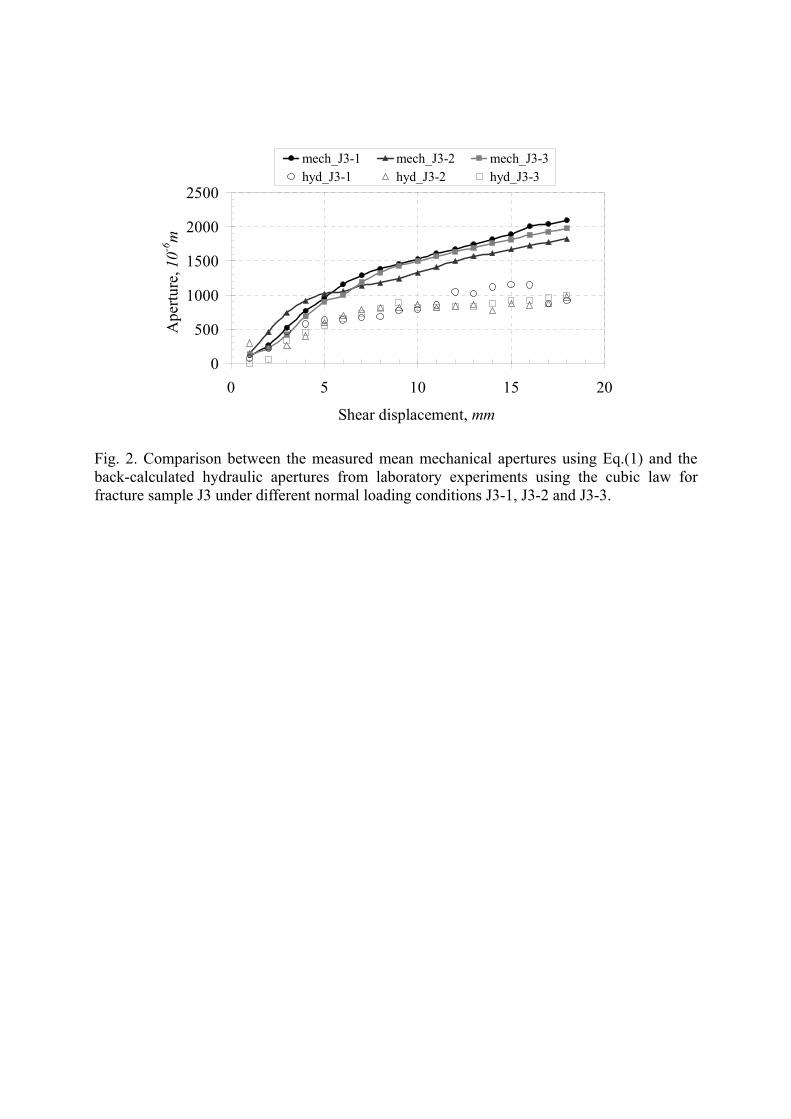
During the shear-flow tests, the mean mechanical aperture, bm, was assessed based on

measured values of the items in the following equation [1]:

snm bbbb ∆+∆−= 0 (1)

where b0 is the initial aperture, ∆bn is the change of aperture by normal loading (such as

closure or opening), and ∆bs is the change of aperture by shearing (dilation). The initial

aperture b0 under a certain normal stress can be obtained by using the normal stress-normal

- 8 -

displacement curves (which are usually fitted by a hyperbolic function) when initial stress

state is available. Under the CNL boundary conditions, ∆bn could be taken as a constant, and

∆bs is the measured normal displacement (dilation) during shear. For the tests under the CNS

boundary conditions, the normal stress changes with both the normal and shear displacements,

therefore, ∆bn itself should be revised due to the corresponding normal stress during shear and

∆bs is also the measured normal displacement (shear dilation). The evaluated mean normal

displacement of the sample during shear is then used in the numerical simulations for

evaluating shear-induced changes of mechanical apertures of elements in the FEM models.

The mean mechanical apertures calculated from measured topographical data using Eq.(1)

and the back-calculated hydraulic aperture from experimental flow fate data using cubic law

for fracture sample J3 under different normal loading conditions (a constant normal stress of

1.0 MPa for J3-1, normal stiffness of 0.2 GPa/m with an initial normal stress of 1.0 MPa for

J3-2 and normal stiffness of 0.5 GPa/m with an initial stiffness of 1.0 MPa for J3-3,

respectively) are compared in Table 2 and Fig. 2. Both the mean mechanical aperture and the

back calculated hydraulic aperture increase with increasing shear displacements (due to the

shear dilation) and decreases with increasing normal stresses, respectively. However the mean

mechanical aperture is always larger than the hydraulic aperture. This is due to the fact that

fluid flow occurs only in connected voids bypassing contact areas. This agrees well with

commonly adopted physical behaviour of rough rock fractures. Note that when normal

stiffness is applied, normal stress will increase with shear displacement by shear-induced

normal dilation. Therefore normal stresses in J3-2 and J3-3 are not constant but increase

gradually with shear displacement, and larger than the initial normal stress of 1.0 MPa that is

also the constant normal stress condition for J3-1. Therefore apertures of J3-2 and J3-3 are

smaller at each shear state comparing with that of J3-1. The increased asperity deformation by

- 9 -

stiffness induced normal stress increase was not considered in this study for simplicity, but

will be considered in future works.

3. Numerical simulations

3.1 Governing equations

When flow velocity is low and the fracture surface geometry does not vary too abruptly the

Reynolds equation can be used, instead of the full Navier-Stokes equations, to describe the

flow in fractures [16, 22]. Assuming that the flow of an incompressible fluid through the

fracture follows the cubic law, in a steady state, the governing equation can be written as

0=+

∂∂

∂∂

+

∂∂

∂∂ Q

yhT

yxhT

x yyxx (2)

where Q is the source/sink term (positive when fluid is flowing into the fracture), and Txx and

Tyy are the fracture transmissivity in x- and y- directions, respectively. In this paper, the local

transmissivity at each point is assumed to be equal in x- and y- directions for simplicity and is

defined by

( )µ

ρ12

,3gb

yxTTT fyyxx === , (3)

where µ is the dynamic viscosity, fρ the fluid density, g the gravitational acceleration,

and b the local fracture aperture (calculated using Eq.(1)), respectively. The local

transmissivity of the fracture can be determined element by element, according to the aperture

evaluation results. In this study, the density and dynamic viscosity of water at 10°C were used

- 10 -

as fρ = 3210997.9 mkg× and µ = sPa ⋅× −310307.1 , respectively, with a gravitational

acceleration g = 2807.9 sm .

Applying the Galerkin scheme to the Eq. (2), the discretized FEM formulation of the above

governing equation becomes

( )[ ] ( ){ } ( ){ }∑∑==

=N

m

mN

m

mm FhK11

, (4)

with

( )[ ] ( )[ ] ( )[ ]( )( )[ ]dSBDBK m

S

mmmm∫=

T , (5)

( ){ } ( )[ ]( )( ) ( )[ ]( ) dLn

yhTn

xhTNdSQNF yxL

mm

S

mmmm

∂∂

+∂∂

−= ∫∫TT

, (6)

where N is the total number of elements, m the element number, and [K(m)], {h(m)}, {F(m)},

[N(m)], S(m) and L(m) are the local transmissivity matrix, hydraulic head vector, flux vector,

shape function matrix, surface area and the boundary in which the flow rate is known for

element m, respectively. The symbols nx and ny are the unit normal vector components to the

boundary in x and y-direction, respectively. The matrices [D(m)] and [B(m)] are defined as

( )[ ]( )

( )

=

=

µρ

µρ

120

012

00

3

3

mf

mf

m

gb

gb

TT

D (7)

( )[ ]( )[ ]

( ){ } ( )[ ] ( ){ }mmmm

m

hBh

yN

xN

yhxh

=

∂∂

∂∂

=

∂∂∂∂

T

T

(8)

To solve Eq. (4), the commercial FEM software, COMSOL Multiphysics [23] was used to

simulate flow processes during shear in this study. Since the number of the scanning points on

- 11 -

the surface for representing the roughness and calculating the aperture is very large (2000 ×

1000 points) for each sample, even though they are regularly distributed over the specimen

area, the digitalized aperture fields of the fracture specimens were divided into 20000 (200 ×

100) small square grids of an edge length of 1.0 mm. The mean aperture of each grid zone

was calculated at each shear displacement interval (1.0 mm). Numerical shearing is simulated

by moving the upper surface by a horizontal translation of 1 mm in the shear direction, then

uplifting by the dilation increment according to the measured mean shear dilation value at that

shear interval. Since initial aperture is zero for fully mated specimens, full contact is assumed

everywhere with zero aperture as the initial condition in the numerical simulations. When

translational shear and dilation displacements are enforced during the numerical simulations

of shearing processes as mentioned above, the previous full contact pattern is broken and

some new voids and new contact areas are generated and the contact conditions and apertures

must be re-evaluated for all grid zones. When a zone has its two opposing surfaces separated,

it represents a void zone and its aperture is evaluated as the mean distance in the direction

normal to the mean plane of the fracture. When its two opposing surfaces are just in touch or

penetrate each other with negative values of contact distance, which represents a contact zone

and is assigned with a zero aperture. In reality the latter represents surface damage/asperity

degradation. The degree of such approximation depends much on the scanning grid mesh

resolution of the fracture surface and the chosen FEM model mesh. Some compromises and

simplifications must be adopted to make a reasonable size of the FEM model for flow

simulations. All void zones as assumed to be parallel plate models obeying the cubic law with

a constant mean aperture. Please note that in the reality of tests, perfect full contact may or

may not be realized since relocation errors (putting two opposite surfaces to their assumed

initial relative positions) always exist, to varying extent.

- 12 -

In the numerical modeling of fluid flow, effect of gorge materials is ignored since negligible

amount of gorge materials were observed during tests. Asperity deformation was not

considered but damage at contact points were partially approximated by removing the

overlapping parts of contacting asperities in the contact elements. Their effects on shear

dilation and fluid flow are, however, reflected in the measured total flow rate and normal

displacement values. Because of the fully mated initial conditions of samples, the

shear-induced dilation became the only contribution mechanism to the changes of aperture

and served as the controlling parameters for the evolutions of aperture/transmissivity fields.

The special treatment of the contact areas for the flow simulation is described in the next

section. Since irregular triangle elements were used in the COMSOL modeling for fluid flow,

which is more flexible for treatment of the complex contact geometry with much finer FEM

meshes around the contact areas, the regular rectangular grid aperture data evaluated using the

approach described above paragraph was linearly interpolated for the triangle elements. This

technique was applied to evaluate the elemental transmissivity, which can be calculated from

aperture value using Eq. (3), assuming local validity of the Reynolds equation, at each shear

displacement interval to simulate the fluid flow through the fracture during shear.

3.2 Boundary conditions and the treatment of contact areas

Unidirectional flow parallel with the shear direction was considered in the tests by fixing the

initial hydraulic heads of 0.1 m and 0 m along the left- and right-hand boundaries,

respectively (see Fig. 3a). This flow boundary condition is the same as the one used in the

laboratory coupled shear-flow tests, which was presented in the previous works by the authors

[6, 7]. For the contact areas, once zero values are given to the aperture, all components of the

- 13 -

calculated local transmissivity matrix, [K(m)] in Eq. (5) becomes zero and assemblage of the

local transmissivity matrix becomes singular. Therefore, Eq. (4) cannot be solved without

special treatment. One usually adopted numerical technique to avoid such singularities is to

assign very small aperture values to the contact elements to generate non-singular

transmissivity matrices [17, 20-21]. However, by giving these artificial, even very small,

transmissivity values for the elements in contact areas, due to their high resistance to the fluid

flow, large hydraulic head drop will occur inside the contact areas. As a result, iso-potential

contour lines become very dense through them and some flow, even very small, still exists

inside the contact areas. This may not affect the calculations of global hydraulic variables

such as the mean flow rates. However, it may affect the local pattern of the streamlines

around the contact areas and give artificial changes to the particle transport paths that may

change the travel distances and time, dispersion and tortuosity. Hence, in this study, contact

areas/elements were numerically eliminated from the calculation domain and their boundaries

were treated as additional internal boundaries with a zero flux condition ( ) 0=⋅∇≡∂∂ nhnh ,

where n is the outward unit normal vector, in order to satisfy conditions of no flow into or out

of the contact areas [14], as shown in Fig. 3a. This processes for finding contact areas,

eliminating them from the element assemblage process and treating them as internal no-flux

boundaries was done automatically by using a CAD system. Once the updated calculation

domain with contact areas treated as additional boundary conditions, it is straightforward to

apply the geometrical and the external/internal boundary conditions in the FEM models

suitable for the COMSOL code for flow simulations. One of the FEM mesh of the fracture

specimen thus generated for fluid flow simulations in this study is shown in Fig. 3b. The use

of irregular triangle mesh to quantify the elemental hydraulic transmissivities is explained in

Section 3.1.

- 14 -

4. Results

4.1 Aperture, transmissivity and contact area evolutions during shear

Figure 4 show the evolution of transmissivity fields of sample J3 under different normal

loading conditions: J3-1, J3-2 and J3-3. In the figure, the white ‘islands’ indicate the contact

areas. The grey intensity of the background in the flow areas indicates the magnitude of local

transmissivities (see the legend in the figures). The simulation results show that shear induced

new contact areas decrease slowly with increasing shear displacement (from full contact as

the initial condition), reach a critical value at about 2 mm of shear displacements, decrease

sharply afterwards and become almost constant after shear displacement of 5 mm (Fig. 4a, c),

with the number of contact spots becoming much smaller and focused at a much fewer

locations of larger areas of contact. Figure 5 shows the measured shear stress and normal

displacement (dilation) curves during shear. The oscillations of small magnitudes in the stress

curves are probably due to the interactions between the samples and testing frame, and

asperity damage on the fracture sample surfaces. A good correspondence can be observed

between the development stages of contact areas and the shear stress (Fig. 5a) and shear

dilation curves (Fig. 5b). The critical total area of contact at a shear displacement of 2 mm,

indicating the maximum mobilized contact areas (Fig. 4), corresponds to the occurrence of the

peak shear stress at the same shear displacement (Fig. 5a) and the first upward turning point

of the shear dilation curve (Fig. 5b). Continuous increase of the shear dilation indicates

continuous increase of the aperture, as indicated also in Fig. 2. It is important to note that at

all stages the distributions of contact spots are relatively uniform, indicating the

homogenization for calculating the mean values of hydraulic properties is reasonable. Such

- 15 -

basis for homogenization may not exist if fractures have dominating structural

non-stationarities (such as large scale asperities clustered at one or two spots).

These figures clearly show the influences of initial morphological behaviors of rock fractures

and the normal loading effects on the development of transmissivity.

4.2 Flow simulation results

The simulated results of flow velocities are superimposed in Fig. 4, with arrows, at different

shear displacement of 1, 2, 5 and 10 mm for fracture J3 under different normal loading

conditions (J3-1, J3-2 and J3-3, respectively). Since the samples are assumed to be fully

mated with a zero initial aperture, no flow is possible at the start. At 1 mm of shear

displacement, the contact areas are widely and uniformly distributed over the whole fracture

sample with small fluid flow at a number of outlet spots without major flow path (first figure

of Figs. 4a, b and c). More continuous flow paths start to form at 2 mm of shear

displacements, and continue to grow into main flow paths with continued decrease of contact

areas and increase of transmissivity, with increasing shear displacement (see the last three

figures of Figs. 4a, b, and c), with only one outlet spot on the outlet boundary of the samples,

with the widely distributed contact areas and complicated void space geometry, which causes

complex structure of transmissivity and flow velocity fields. As a result, flow patterns (or

stream lines) become very tortuous. This phenomenon is the well-known ‘channelling effect’

[24]. At present only numerical simulations can illustrate realistically the process of complex

evolution of the flow localization (channeling) during shear under different normal loading

conditions, since direct measurement and visualization is not possible.

- 16 -

The flow rate at the outlet boundary (along x=0) of sample J3 with different normal loading

conditions were compared between laboratory tests and numerical simulations as shown in

Fig. 6 and Table 3. Note that the zero flow rates cannot be plotted in the figure with

log-scaling in the axis for flow rate. The general behaviors of the simulated flow rate

variations with shear displacements under different normal stress/stiffness conditions were

captured for all three conditions of normal loading, agree well with measured results. Both

simulated and measured flow rates show the sharp increase at about 2 mm shear

displacements and continue to increase but with a progressive reduction of gradient, and more

stabilized flow rate after the 5 mm shear displacement, corresponding to the almost stabilized

contact areas as shown in Fig. 4. The general increase of flow rate is about 5-6 orders of

magnitude from the initial state before shear. The maximum increase of flow rate is between

10-5-10-4 m3/sec in order of magnitude. These general behaviors agree with the general

understanding of the flow behavior of rock fractures. Please note that the numerical

simulation was not calibrated with test results but predictions with assumptions of zero

apertures (therefore zero flow rate) as the initial state for all cases. But in test, non-zero flow

rate was observed in J3-3, with possible relocation errors that were not considered in

numerical predictions.

The results presented here are more realistic, due to more proper treatment of contact areas in

flow simulations, compared with earlier results reported in literature, obtained from flow

simulations in which fracture samples have only a few very small contact areas, without

normal stress or with very small normal stresses [16-19].

The measured hydraulic apertures of the fractures and their evolutions during shear were back

calculated from the flow rates obtained from laboratory tests are compared with the predicted

values by numerical simulations in Fig. 7, and tabulated in Table 4. The measured and

predicted values agree well, even with non-zero initial apertures during tests. The magnitudes

- 17 -

of the predicted hydraulic apertures are systematically slightly larger than the measured ones

due to the fact that deformation and damage of asperities on fracture surface and generation of

gorge materials were not considered in the numerical predictions so that the measured flow

rates should be smaller than the simulated ones, but the discrepancy is well within acceptable

small ranges corresponding to mechanical deformation/damage effects. Both the numerical

predictions and the measured aperture data show that with increasing normal stresses in the

order of J3-1, J3-3 and J3-2 in terms of normal stress magnitude, apertures decreases

accordingly in the same order. This agrees well with commonly adopted physical behaviour

of rough rock fractures. The small offset between the results in J3-2 and J3-3 are due to

changes in test conditions occurred during tests (such as consistency in fluid sealing at

different shear stages and initial sample relocation offsets, etc.).

The deviations in flow rates and hydraulic apertures between the experimental results and

numerical predictions may be caused by three possible reasons that were not considered in

numerical simulations:

1) uneven dilation in the fracture (tilting of the fracture samples, for example) during

coupled shear-flow tests;

2) relocation offsets by experimental difficulties to realize fully mated initial condition with

very small fluid flow still exists for J3-1 and J3-2 even after applying weak cyclic normal

loading during tests (see Figs. 6 and 7 and Tables 3 and 4);

3) mechanical deformation and damage of asperities and thus generated gorge materials.

Among the above reasons as possible sources of discrepancies in the results of flow rates and

hydraulic apertures, the ignorance of asperity deformation are the most significant, since

generation of gorge materials by damage is not significant as observed in tests. The relocation

error (offset) is of the secondary importance since it affects mainly the general behaviors of

- 18 -

simulation results in early stage of shear, before 2 mm of shear displacement. The effects of

relocation offset and tilting could be considered readily in further model calibrations as long

as the initial aperture and tilting direction and extent can be quantified during testing, but the

asperity deformation and damage cannot be properly considered at present.

5. Discussions and concluding remarks

In the present study, the fluid flow in rock fracture replicas during shear under normal stress

and normal stiffness controls was simulated using the COMSOL Multiphysics code of FEM

with a special algorism for contact areas, considering evolutions of aperture and

transmissivity fields during shear, obtained from real coupled shear-flow tests of fracture

specimens of realistic surface roughness features. The numerical models captured complex

behavior of fluid flow in fracture samples with special highlights in terms of contact area

evolutions using the special algorithm of contact elements of zero apertures. This contact

algorithm is an important link for realistic simulations of couplings between stress and fluid

flow in fractures with shear and under normal loading. The results show that such special

treatment of contact areas can simulate more realistic behaviour of flow fields in fractures that

is important for particle transport simulations.

Besides the above general conclusions, a few outstanding issues need to be further discussed.

a) Validity of Reynolds equation (the cubic law)

The Navier-Stokes equations have been solved using FEM in real fracture geometry,

considering non-linear regimes of fluid flow in rock fractures, with results compared to

experiments, as reported in [25]. The Reynolds equation, on the other hand, is more

- 19 -

commonly used for the flow in fractures for its simplicity, as demonstrated by many

publications, under certain conditions of hydraulic gradient, aperture, fluid velocity, etc.,

depending on the Reynolds number of the flow fields. We used it for simplicity in this work

since effects of normal stress and shear displacement on fluid flow in fractures are the causes

of first order variations and are therefore the main concern, and believed that the Reynolds

equation could be acceptable for all shear displacement stages. To check whether our

assumption is valid, we calculated the Reynolds numbers of the measured flow data during

the tests, as listed in Table 5. The resultant Reynolds numbers generally satisfies the

requirements for laminar steady state flows, as we assumed. Therefore, use of Reynolds

equation for solving the flow and back-calculating the hydraulic properties can be accepted.

b) Technical difficulties of measuring evolutions of aperture during shear

The accurate knowledge of aperture evolution under normal loading during shear is important

for the development of coupled hydro-mechanical constitutive models for rock fractures. To

get accurate aperture values during shear, direct measurement is desirable but not possible in

practice in laboratory tests at present. The most common way to obtain the mean aperture in

numerical modeling is to calculate the distance of superimposed two rough surfaces in the

direction perpendicular to the nominal fracture plane, which is adopted in this study, and

back-calculation using measured flow rate in tests assuming validity of the cubic law.

However, some assumptions are always required to determine the initial position of rough

surfaces corresponding to the samples’ in situ stress conditions, to quantify the local aperture

distribution, and to estimate relocation errors. More accurate measurement of relocation errors

at the start and quantification of tilting effects during shear are important for more accurate

numerical predictions, especially for rough fracture samples not fully mated at the initial

conditions.

- 20 -

c) The asperity degradation/damage and generation of gorge materials cannot be measured at

asperity scale directly during shear tests, due to the same technical difficulty as the

determination of aperture field during shear. However, as demonstrated in this paper, they

have significant effects on fluid flow in rock fractures. More development in numerical

modelling with functions of stress, deformation and damage analyses are needed to improve

the capacity of more reliable numerical modelling tools. On the other hand, development of

more advanced experimental techniques for quantitative real-time measurement of evolution

of aperture and surface roughness during shear with normal loading, in conjunction with fluid

flow, however, is needed not only to validate numerical models, but also for the scientific

foundation of the subject.

d) Effect of proper treatment of contact areas

The iso-value contours of hydraulic head for fracture sample J3 under constant normal stress

of 1.0 MPa (test case J3-1) at a shear displacement of 5 mm are compared between with and

without special treatment for contact areas in Fig. 8. It should be noted that very small

aperture value of 0.1 µm was given for the contact areas for the case of without special

treatment, as shown in Fig. 8b. Figure 8a shows the results with special contact elements

developed in Section 3.2. The calculated overall flow rates were almost the same between the

two models. However, as shown in Fig. 8b, some of the iso-value contours of hydraulic head

crossed the contact areas and caused continuous and tightly clustered zones with very small

aperture values (Fig. 8b), which is physically not meaningful. Such continuous clusters will

not form when zero apertures were given to contact elements (Fig. 8a), with iso-value contour

lines stopping right at the boundary of the contact areas in right angles, forming a much

discontinuous overall pattern of the iso-value contour lines of hydraulic head. This difference

- 21 -

in the overall pattern of continuously clustered or broken clusters of iso-head contour lines

will affect local stream lines around the contact areas and change the particle transport paths

and travel time, such as trapping particles, and changing tortuosity of stream lines, which will

affect the final calculation of break through curves and evaluation of the transport properties

in the fractures [26].

Acknowledgement

The authors thank the Swedish Nuclear Power Inspectorate (SKI) for the financial support for

the first author’s Ph.D studies at Royal Institute of Technology (KTH), Stockholm, Sweden.

References

[1] Esaki T, Du S, Mitani Y, Ikusada K and Jing L. Development of a shear-flow test

apparatus and determination of coupled properties for a single rock joint. Int J Rock Mech

Min Sci 1999; 36: 641-50.

[2] Olsson R, Barton N. An improved model for hydromechanical coupling during shearing of

rock joints. Int J Rock Mech Min Sci, 2001; 38: 317-329.

[3] Lee HS and Cho TF. Hydraulic characteristics of rough fractures in linear flow under

normal and shear load. Rock Mech Rock Engng, 2002; 35: 299-318.

[4] Hans J and Boulon M. A new device for investigating the hydro-mechanical properties of

rock joints. Int J Numer Anal Meth Geomech, 2003; 27: 513-548.

- 22 -

[5] Auradou H, Drazer G, Hulin JP and Koplik J. Permeaqbility anisotropy induced by the

shear displacement of rough fracture walls. Water Resour Res, 2005; 41: W09423, doi:

10.1029/2005WR003938.

[6] Li B, Jiang Y, Saho R, Tasaku Y and Tanabashi Y. An investigation of hydromechanical

behaviour and transportability of rock joints. In: Rock Mechanics in Underground

Construction, Proc of the 4th Asian Rock Mech Symp, eds. Leung CF Y and Zhou YX,

World Scientific, 2006, pp. 321.

[7] Li B, Jiang Y, Koyama T, Jing L and Tanabashi Y. Experimental study on

hydro-mechanical behaviour of rock joints by using parallel-plates model containing

contact area and artificial fractures. Manuscript submitted to Int J Rock Mech Min Sci,

October, 2006.

[8] Jiang Y, Xiao J, Tanabashi Y and Mizokami T. Development of an automated

servo-controlled direct shear apparatus applying a constant normal stiffness condition. Int

J Rock Mech Min Sci, 2004; 41(2): 275-286.

[9] Jiang Y, Li B and Tanabashi Y. Estimating the relation between surface roughness and

mechanical properties of rock joints. Int J Rock Mech Min Sci, 2006; 43(6): 837-846.

[10] Brown SR, Caprihan A and Hardy R. Experimental observation of fluid flow channels in

a single fracture. J Geophys Res, 1998; 103(B3): 5125-5132.

[11] Detwiler RL, Pringle SE and Glass RJ. Measurement of fracture aperture fields using

transmitted light: An evaluation of measurement errors and their influence on simulations

of flow and transport through a single fracture. Water Resour Res, 1999; 35(9):

2605-2617.

[12] Renshaw CE, Dadakis JS and Brown SR. Measuring fracture apertures: A comparison of

methods. Geophys Res Lett, 2000; 27(2); 289-292.

- 23 -

[13] Xiao J, Satou H, Sawada A and Takebe A. Visualization and quantitative evaluation of

aperture distribution, fluid flow and tracer transport in a variable aperture fracture. In:

Rock Mechanics in Underground Construction, Proc of the 4th Asian Rock Mech Symp,

eds. Leung CF Y and Zhou YX, World Scientific, 2006, pp. 416.

[14] Zimmerman RW, Chen DW and Cook NGW. The effect of contact area on the

permeability of fractures. J Hydrology, 1992; 139: 79-96.

[15] Lespinasse M and Sausse J. Quantification of fluid flow: hydro-mechanical behaviour of

different natural rough fractures. J Geochemical Exploration, 2000; 60-70: 483-486.

[16] Yeo IW, De Freitas MH and Zimmerman RW. Effect of shear displacement on the

aperture and permeability of rock. Int J Rock Mech Min Sci, 1998; 35: 1051-70.

[17] Kim HM, Inoue J and Horii H. Flow analysis of jointed rock masses based on

excavation-induced transmissivity change of rough joints. Int J Rock Mech Min Sci, 2004;

41(6): 959-974.

[18] Koyama T, Fardin N, Jing L and Stephansson O. Numerical simulation of shear induced

flow anisotropy and scale dependent aperture and transmissivity evolutions of fracture

replicas. Int J Rock Mech Min Sci, 2006; 43(1): 89-106.

[19] Matsuki K, Chida Y, Sakaguchi K and Glover PWJ. Size effect on aperture and

permeability of a fracture as estimated in large synthetic fractures. Int J Rock Mech Min

Sci, 2006; 43(5): 726-755.

[20] Brown SR. Fluid flow through rock joints: The effects of surface roughness. J Geophys

Res, 1987; 92(B2): 1337-1347.

[21] Yasuhara H and Elsworth D. A numerical model simulating reactive transport and

evolution of fracture permeability. Int J Numer Anal Meth Geomech, 2006; 30:

1039-1062.

- 24 -

[22] Zimmerman RW and Bodvarsson GS. Hydraulic conductivity of rock fractures. Transp

Porous Media, 1996; 23: 1-30.

[23] COMSOL AB. COMSOL Multiphysics Ver.3.3, Stockholm, 2006. Home page:

http://www.comsol.se

[24] Tsang YW and Tsang CF. Channels model of flow through fractured media. Water

Resour Res, 1987; 23(3): 467-479.

[25] Zimmerman RW, Al-Yaarubi A, Pain CC, and Grattoni CA. Non-linear regimes of fluid

flow in rock fractures. Int J Rock Mech Min Sci, 2004; 41(3): 384-384.

[26] Koyama T, Vilarrassa V, Neretnieks I and Jing L. Shear-induced Flow Channels in a

Single Rock Fracture and their Effect on Particle Transport, Manuscript submitted to

Water Resour Res, March, 2006.

Table 1. Experimental loading cases under CNL and CNS boundary conditions for sample J3.

* CNL: Constant Normal Load (stress) and CNS: Constant Normal Stiffness Table 2. Comparison between mean mechanical apertures and the back-calculated hydraulic apertures using the cubic law in laboratory experiments for fracture sample J3. See Table 1 for different normal loading conditions.

(unit: µm) J3-1 (CNL, 1.0 MPa) J3-2 (CNS, 0.2 GPa/m) J3-3 (CNS, 0.5 GPa/m) Shear

disp. mm mechanical hydraulic mechanical hydraulic mechanical hydraulic1 119.171 78.0141 145.072 299.120 129.5993 02 262.980 226.743 458.592 248.122 222.0791 55.49603 519.278 467.933 742.291 263.580 423.1777 327.9784 767.296 578.374 918.687 399.546 686.6003 450.3455 950.857 631.659 1019.99 596.297 900.3918 552.6656 1153.02 637.699 1053.64 698.376 999.3655 654.9257 1285.95 669.418 1134.24 785.275 1189.439 728.1888 1381.37 687.352 1177.96 810.937 1323.947 794.4999 1451.52 771.911 1240.91 821.197 1426.133 889.394

10 1524.01 786.980 1325.06 860.159 1499.285 813.60211 1607.74 849.646 1410.14 822.820 1563.727 817.56712 1668.77 1044.16 1497.07 840.610 1630.976 837.68513 1741.27 1019.65 1568.72 858.203 1687.956 832.30614 1815.91 1117.41 1611.59 773.331 1758.472 873.32815 1889.49 1154.70 1669.24 875.828 1810.214 921.09116 2004.69 1146.49 1725.01 853.338 1876.390 918.96317 2037.89 875.277 1771.20 871.887 1924.038 964.50518 2090.96 919.616 1821.15 970.137 1977.605 996.645

Normal loading conditions Fracture Samples

Loading cases

Roughness (JRC range) *CNL/CNS Initial normal stresses, σni

(MPa) Normal stiffness, kn

(GPa/m)

J3 J3-1 J3-2 J3-3

16~18 CNL CNS CNS

1.0 1.0 1.0

0 0.2 0.5

Table 3. Comparison of the mean flow rates at sample outlets between laboratory experiments and numerical simulations for fracture sample J3. See Table 1 for different normal loading conditions.

(unit: m3/sec) J3-1 (CNL, 1.0 MPa) J3-2 (CNS, 0.2 GPa/m) J3-3 (CNS, 0.5 GPa/m) Shear

disp. mm Experiments Simulation Experiments Simulation Experiments Simulation0 3.58724e-08 0 8.97865e-07 0 0 01 1.49147e-08 6.81190e-09 8.40683e-07 2.33799e-08 0 1.22573e-082 3.68031e-07 1.10853e-07 4.82259e-07 1.20040e-06 5.39595e-09 3.40911e-083 3.25112e-06 1.32808e-06 5.81058e-07 6.33769e-06 1.11948e-06 5.18847e-075 8.07910e-06 1.39717e-05 6.79677e-06 1.31203e-05 5.41128e-06 7.26221e-067 9.71590e-06 2.45841e-05 1.56840e-05 1.48290e-05 1.25061e-05 1.71328e-05

10 1.60356e-05 3.78310e-05 2.09378e-05 1.78881e-05 1.77187e-05 3.52597e-0515 5.20220e-05 7.39862e-05 2.27004e-05 3.56260e-05 2.64049e-05 5.83768e-0518 2.67115e-05 1.02628e-04 3.13601e-05 5.02597e-05 3.40015e-05 7.67927e-05

Table 4. Comparison of the hydraulic apertures between laboratory measurements (from flow rates using cubic law) and numerical simulations for fracture sample J3. See Table 1 for different normal loading conditions.

(unit: µm) J3-1 (CNL, 1.0 MPa) J3-2 (CNS, 0.2 GPa/m) J3-3 (CNS, 0.5 GPa/m) Shear

disp. mm Experiments Simulation Experiments Simulation Experiments Simulation0 104.700 0 306.265 0 0 01 78.0141 60.0792 299.120 90.6252 0 73.07452 226.743 151.992 248.122 336.264 55.4960 102.5933 467.933 347.200 263.580 584.542 327.978 253.8165 631.659 758.191 596.297 742.466 552.665 609.6097 669.418 912.195 785.275 770.738 728.188 808.746

10 786.980 1047.65 860.159 816.187 813.602 1023.3615 1154.70 1298.55 875.828 1017.80 921.091 1199.9318 919.616 1440.33 970.137 1135.31 996.645 1307.62

Table 5. Calculated Reynolds numbers of the flow in the test conditions of sample J3 Shear disp. mm J3-1 (CNL, 1.0 MPa) J3-2 (CNS, 0.2 GPa/m) J3-3 (CNS, 0.5 GPa/m)

0 0.27438 6.867605 0 1 0.11408 6.430231 0 2 2.81500 3.688709 0.041273 3 24.8672 4.444403 8.562729 5 61.7956 51.98725 41.38984 7 74.3151 119.9642 95.65674

10 122.654 160.1494 135.5272 15 397.907 173.6314 201.9662 18 204.311 239.8675 260.0714

Fig. 1. 3-D surface topography model of fracture specimen J3 based on the laser scanning results. It should be noted that the resolution of the figures was reduced up to mesh size of 2 mm.

(mm)

0

500

1000

1500

2000

2500

0 5 10 15 20

Shear displacement, mm

Ape

rture

, 10-6

mmech_J3-1 mech_J3-2 mech_J3-3hyd_J3-1 hyd_J3-2 hyd_J3-3

Fig. 2. Comparison between the measured mean mechanical apertures using Eq.(1) and the back-calculated hydraulic apertures from laboratory experiments using the cubic law for fracture sample J3 under different normal loading conditions J3-1, J3-2 and J3-3.

Fig. 3. Special treatment for the contact areas, a) Boundary conditions for flow simulations and b) the calculation mesh of a FEM model.

h=0 m

h=0.1 m

No flow

Contact areas

No flow

a)

b)

x

y

No flow

1 mm

2 mm

5 mm

10 mm a) b)

1 mm

2 mm

5 mm

10 mm

Fig. 4. Flow velocity fields with transmissivity evolutions at different shear displacements of 1, 2, 5 and 10 mm for fracture sample J3 under different normal loading conditions: a) constant normal stress of 1 MPa, J3-1, b) mixed initial normal stress (1.0 MPa) and normal stiffness (0.2 GPa/m), J3-2 and c) mixed initial normal stress (1.0 MPa) and normal stiffness (0.5 Gpa), J3-3. The white ‘islands’ show contact areas and the legend shows the order of transmissivity (m2/sec).

1 mm

2 mm

5 mm

10 mm c)

0

-2

-4

-6

-8

-10

-12

Min: -13

Max: 0

Fig. 5. Direct shear test results on sample J3: a) the shear stress versus shear displacement and b) the normal displacement versus shear displacement [6, 7].

00.20.40.60.8

11.2

0 2 4 6 8 10 12 14 16 18 20Shear displacement (mm)

Shea

r stre

ss (M

Pa) J3-1

J3-2J3-3

-0.5

0.5

1.5

2.5

0 2 4 6 8 10 12 14 16 18 20Shear displacement (mm)

Nor

mal

dis

plac

emen

t(m

m)

J3-1J3-2J3-3

1.0E-09

1.0E-08

1.0E-07

1.0E-06

1.0E-05

1.0E-04

1.0E-03

0 5 10 15 20

Shear displacement, mm

Flow

rate

, m3 /s

ec

J3-1_experimentJ3-1_simulationJ3-2_experimentJ3-2_simulationJ3-3_experimentJ3-3_simulation

Fig. 6. Comparison of the flow rates at the outlet between laboratory experiments and numerical predictions for fracture sample J3 under different normal loading conditions J3-1, J3-2 and J3-3. It should be noted that zero flow rate values cannot be plotted in the log scale of the flow rate axis, which was assumed at the initial shear stages of modeling.

0200400600800

1000120014001600

0 5 10 15 20

Shear displacement, mm

Hyd

raul

ic a

pertu

re, 1

0-6m

J3-1_experiment J3-1_simulationJ3-2_experiment J3-2_simulationJ3-3_experiment J3-3_simulation

Fig. 7. Comparison of hydraulic apertures back calculated from the flow rates obtained from the experiments (assuming the cubic law) and numerical simulations for sample J3 under different normal loading conditions J3-1, J3-2 and J3-3.

Fig. 8. Iso-value counters of hydraulic head at 5 mm shear displacement a) with and b), without special treatment for contact areas for fracture sample J3 under constant normal stress of 1 MPa, J3-1. Iso-value counters were drawn from 2.5e-4 m to 9.975e-2 m with every 0.5e-4 m intervals. It should be noted that very small aperture value of 0.1 µm was given for contact elements for the case of without special treatment.

b)a)