1  

 

Title: A Metagenomics Portal for a Democratized Sequencing World  

Authors: Andreas Wilke1,2,, Elizabeth M. Glass1,2,, Daniela Bartels1,2, Jared Bischof 1,2, Daniel Braithwaite1,2, Mark D’Souza1,2, Wolfgang Gerlach1,2, Travis Harrison1,2,, Kevin Keegan1,2, Hunter Matthews1, Renzo Kottmann3, Tobias Paczian1,2, Wei Tang, 1,2, William L. Trimble1,2, Pelin Yilmaz3, Jared Wilkening1,2, Narayan Desai1,2, Folker Meyer1,2  1Argonne National Laboratory; 2 University of Chicago; 3Max-Planck Institute für Marine Biologie, Bremen, Germany;  

The democratized world of sequencing is leading to numerous data analysis challenges; MG-RAST solves them for amplicon data sets, shotgun metagenomes, and metatranscriptomes. The changes from version 2 to version 3 include the addition of a dedicated gene calling stage using FragGenescan, clustering of predicted proteins at 90% identity, and the use of BLAT for the computation of similarities. Together with changes in the underlying software infrastructure, this has enabled the dramatic scaling up of pipeline throughput while remaining on a limited hardware budget. The web based service allows upload, fully automated analysis and visualization of results. As a result of the plummeting cost of sequencing and the readily available analytical power of MG-RAST, over 78,000 metagenomic datasets have been analyzed, with over 12,000 of them publicly available in MG-RAST.  

 

Keywords:  

1. automated analysis of metagenomes, metatranscriptomes and amplicon data  

2. public archive for data and analysis results  

3. metadata enabled data discovery  

4. scalable analysis pipeline  

5. next generation sequence analysis  

 

1. INTRODUCTION  

2. Pipeline and technology platform  

Details on the new MG-RAST pipeline  

Additional improvements  

3. WEB INTERFACE  

Overview  

The Upload and Metadata pages  

Metadata enabled data discovery  

2  

 

The Overview Page  

Technical detail on the overview page  

Metagenome QC  

Technical Data  

Taxonomic and functional information on the overview page  

Organism Breakdown  

Functional Breakdown  

The Analysis Page  

Resolving the best hits vs. representative hits conundrum  

Normalization  

Heatmap/Dendrogram  

Ordination  

Table  

KEGG maps  

4. How to drill down using the workbench  

Viewing Evidence  

5. MG-RAST DOWNLOADS  

Uploaded File(s)  

Preprocessing  

Dereplication  

Screening  

Prediction of protein coding sequences  

RNA Clustering  

RNA similarities  

Gene Clustering  

Protein similarities  

6. DISCUSSION  

7. FUTURE WORK  

8. References  

3  

 

9. Acknowledgments  

 

 

1. INTRODUCTION  The growth in data enabled by next-generation sequencing platforms provides an exciting opportunity for studying microbial communities, ~99% of the microbes in which have not yet been cultured (Riesenfeld, Schloss, & Handelsman, 2004). To support user-driven analysis of metagenomic data, we have provided MG-RAST (Meyer, Paarmann, D'Souza, Olson, Glass, Kubal, et al., 2008). The MG-RAST portal offers automated quality control, annotation and comparative analysis services and archives over 78,000 datasets contributed by over 10,000 researchers.  

While the previous version of MG-RAST (v2) was widely used, it was limited to datasets smaller than a few 100 Mbases and comparison of samples was limited to pairwise comparisons. In the new version, datasets of 10s of gigabases can be annotated and comparison of taxa or functions that differed between samples is now limited by the available screen real estate. Figure 1 shows a comparison of the analytical and computational approaches used in MG-RAST v2 and v3. The major changes are the inclusion of a dedicated gene calling stage using FragGenescan (Rho, Tang & Ye, 2010), clustering of predicted proteins at 90% identify using uclust (Edgar, 2010) and the use of BLAT (Kent, 2002) for the computation of similarities. Together with changes in the underlying infrastructure this has allowed dramatic scaling of the analysis with the limited hardware available.  

The new version of MG-RAST represents a rethinking of core processes and data products, as well as new user interface metaphors and a redesigned computational infrastructure. MG-RAST supports a variety of user-driven analyses, including comparisons of many samples, previously too computationally intensive to support for an open user community.  

4  

 

 Figure 1: Overview of processing pipeline in (a) MG-RAST 2 and (b) MG-RAST 3. In the old pipeline, metadata was rudimentary, compute steps were performed on individual reads on a 40-node cluster that was tightly coupled to the system, and similarities were computed by BLAST to yield abundance profiles that could then be compared on a per-sample or per pair basis. In the new pipeline, rich metadata can be uploaded, normalization and feature prediction are performed, faster methods such as BLAT are used to compute similarities, and the resulting abundance profiles are fed into downstream pipelines on the cloud to perform community and metabolic reconstruction and to allow queries according to rich sample and functional metadata.  

Scaling to the new workload required changes in two areas: the underlying infrastructure needed to be re-thought and the analysis pipeline needed to be adapted to address the properties of the newest sequencing technologies.  

2. Pipeline and technology platform  One key aspect of scaling MG-RAST to large numbers of modern NGS datasets is the use of cloud computing which decouples MG-RAST from its previous dedicated hardware resources. Using our task server AWE (Wilke, Wilkening, Glass, Desai, and Meyer, 2011) and the SHOCK data management tool developed alongside it we have updated our underlying computational platform using purpose built software platform optimized for large scale sequence analysis.  

The new analytical pipeline for MG-RAST version 3 (Figure 2) is encapsulated and separated from the data store, enabling far greater scalability.  

 

5  

 

 Figure 2: Details of the analysis pipeline for MG-RAST version 3.x  

Details on the new MG-RAST pipeline  Several key algorithmic improvements were needed to support the flood of user-generated data.  

PREPROCESSING: First, we replaced the read-centric approach, no longer performing a search for each independent read. The new pipeline actually consists of two independent flows. After upload, data is pre-processed using SolexaQA (Cox, Peterson & Biggs, 2010) to trim low quality regions from FASTQ data. Platform specific approaches are used for 454 data submitted in FASTA format: reads more than than two standard deviations away from the mean read length are discarded following (Huse, Huber, Morrison, Sogin & Welch, 2007).  

RNA DETECTION, CLUSTERING, and IDENTIFICATION: rRNA reads are identified using a simple rRNA detection pipeline and are searched in a separate flow in the pipeline. An initial BLAT (Kent, 2002) search against a reduced RNA database efficiently identifies RNA. The RNA-similar reads are then clustered at 97% identity and a BLAT similarity search is performed for the longest cluster representative.  

DEREPLICATION: For the remaining data after quality filtering (which we assume to be protein coding) the processing starts with a de-replication step used to remove artificial duplicate reads (ADRs) (Gomez-Alvarez, Teal & Schmidt, 2009). Instead of discarding the ADRs we use these technical duplicates to estimate an error score for the entire data set based on the variations in the sets of nearly identical reads stemming from artificial duplication (Keegan, Trimble, Wilke, Harrison, D’Souza, & Meyer, 2012).  

QUALITY ASSESSMENT: The MG-RAST pipeline offers a variety of summaries of technical aspects of the sequence quality to enable sequence data triage. These tools include DRISEE for estimating sequence error, summaries of the spectra of long kmers, and visualizations of the base caller output.  

1. DRISEE, (Duplicate Read Inferred Sequencing Error Estimation)  

6  

 

DRISEE (Keegan et al., 2010) is a method to provide a measure for sequencing error for whole genome shotgun metagenomic sequence data that is independent of sequencing technology, and accounts for many of the shortcomings of Phred. It utilizes ADR’s (artifactual/artificial duplicate reads) to generate internal sequence standards from which an overall assessment of sequencing error in a sample is derived. DRISEE values are normally reported as percent error.  DRISEE values can be used to assess the overall quality of sequence samples. DRISEE data are presented on the Overview page for each MG-RAST sample for which a DRISEE profile can be determined. Total DRISEE Error presents the overall DRISEE based assessment of the sample as a percent error:  Total DRISEE Error = base_errors/total_bases * 100  where “base_errors” refers to the sum of DRISEE detected errors and total_bases refers to the sum of all bases considered by DRISEE.  The current implementation of DRISEE is not suitable for amplicon sequencing data, or other samples that may contain natural duplicated sequences (e.g. eukaryotic DNA where gene duplication and other forms of highly repetitive sequences are common) in high abundance.  

 2. Kmer profiles  k-mer digests are an annotation-independent method to describe sequence datasets that can support inferences about genome size and coverage. Here the overview page presents several visualizations of the kmer spectrum of each dataset, evaluated at k=15.  Three visualizations provided of the kmer spectrum are the kmer spectrum, kmer rank abundance, and ranked kmer consumed. All three graphs represent the same spectrum, but in different ways. The kmer spectrum plots the number of distinct kmers against kmer coverage. The kmer coverage is equivalent to number of observations of each kmer. The kmer rank abundance plots the relationship between kmer coverage and the kmer rank–answering the quesiton “what is the coverage of the nth most-abundant kmer.” Ranked kmer consumed plots the largest fraction of the data explained by the nth most abundant kmers only.  

 3. Nucleotide histograms  These graphs show the fraction of base pairs of each type (A, C, G, T, or ambiguous base “N”) at each position starting from the beginning of each read. Amplicon datasets (see Figure 3) should show biased distributions of bases at each position, reflecting both conservation and variability in the recovered sequences:  

 

7  

 

 Figure 3. Nucleotide histogram with biased distributions.    

Shotgun datasets should have roughly equal proportions of A, T, G and C basecalls, independent of position in the read as shown in Figure 4.  

 Figure 4. Nucleotide histogram showing ideal distributions.  

 Vertical bars at the beginning of the read indicate untrimmed (see Figure 5), contiguous barcodes. Gene calling via FragGeneScan (Rho, 2010) and RNA similarity searches are not impacted by the presence of barcodes. However if a significant fraction of the reads is consumed by barcodes it reduces the biological information contained in the reads.  

 

 Figure 5. Nucleotide histogram with untrimmed barcodes.    

If a shotgun dataset has clear patterns in the data (see Figure 6), this indicates likely contamination with artificial sequences. This dataset had a large fraction of adapter dimers:  

 

8  

 

 Figure 6. Nucleotide histogram with contamination.  

 

SCREENING: The pipeline provides the option to remove reads that are near-exact matches to the genomes of a handful of model organisms, including fly, mouse, cow, and human. The screening stage uses bowtie (Langmead, Trapnell, Pop & Salzberg, 2009) and only reads that do not match the model organisms pass into the next stage of the annotation pipeline.  

GENE PREDICTION and AA Clustering: While the previous version of MG-RAST used similarity-based gene predictions, this approach is significantly more expensive computationally than de-novo gene prediction. After an in depth investigation of tool performance (Trimble, Keegan, D’Souza, Wilke, Wilkening, Gilbert, et al., 2012), we have moved to a machine learning approach: FragGeneScan (Rho et al., 2010). Using this approach we can now predict coding regions in DNA sequences of 75 bp and longer. Our novel approach also enables the analysis of user provided assemblies. MG-RAST builds clusters of proteins at the 90% identity level using the uclust (Edgar 2010) implementation in QIIME (Caporaso, Kuczynski, Stombaugh, Bittinger, Bushman, Costello, et al., 2010) preserving the relative abundances. These clusters greatly reduce the computational burden of comparing all pairs of short reads while clustering at 90% identity preserves sufficient biological signal. Once created, a representative (the longest sequence) for each cluster is subjected to similarity analysis, instead of BLAST we use sBLAT, an implementation of the BLAT algorithm (Kent, 2002), which we parallelized using OpenMPI (Gabriel, Fagg, Bosilca, Angskun, Dongarra, Squyres et al., 2004) for this work.  

Once the similarities are computed we present reconstructions of the species content of the sample based on the similarity results. We reconstruct the putative species composition of the sample by looking at the phylogenetic origin of the database sequences hit by the similarity searches.  PROTEIN IDENTIFICATION and ANNOTATION MAPPING: Sequence similarity searches are computed against a protein database derived from the M5NR (Wilke, Harrison Wilkening, Field, Glass, Kyrpides et al., 2011), which provides a non-redundant integration of many databases (GenBank (Benson, Cavanaugh, Clark, Karsch-Mizrachi, Lipman, Ostell et al., 2012), SEED (Overbeek, Begley, Butler, Choudhuri, Chuang, Cohoon et al., 2005), IMG (Markowitz,  Chen,  Palaniappan,  Chu,  Szeto,  Grechkin  et  al.,  2012), KEGG (Kanehisa, Goto, Sato, Furmichi & Tanabe, 2012), and eggNOGs). Unlike MG-RAST 2, which relied solely on SEED, MG-RAST now supports many complementary views into the data with one similarity search, including different functional hierarchies: SEED subsystems, IMG

9  

 

terms, COG (Tatusov,  Fedorova,  Jackson,  Jacobs,  Kiryutin,  Koonin    et  al.,  2003)/eggNOGs (Jensen,  Julien,  Kuhn,  von  Mering,  Muller,  Doerks  et  al.,  2008) and ontologies such as GO (Gene  Ontology  Consortium, 2013). Users can easily change views without recomputation. For example COG and KEGG views can be displayed, which both show the relative abundances of histidine biosynthesis in a dataset of four cow rumen metagenomes.  

After similarity computation, a number of additional pipeline stages are executed, transforming the data into several representations that enable rapid query and or comparison.  

Additional improvements  Adding the ability for users to encode rich information about each sample is another key improvement in MG-RAST 3. By using the standards developed by the Genomics Standards Consortium we have enabled users to contribute GSC (Field, Amaral-Zettler, Cochrane, Cole, Dawyndt, Garrity et al., 2011) standard formatted metadata. Specifically we use MIxS (Minimum information about any (x) sequence (MIxS) and MIMARKS (Minimum Information about a MARKer gene Survey) specifications (Yilmaz,  Kottmann,  Field,  Knight,  Cole,  Amaral-­‐Zettler et al., 2011) to store metadata and to search for related data sets in terms of geographic location, biochemical environment, or other contextual data.  

This enables data discovery by end-users using contextual metadata using searches like “retrieve soil samples from the continental U.S.”. If the users have added additional metadata (domain specific extension) additional queries are enabled e.g. “restrict the results to soils with a specific pH”.  

We have also enabled users to extract abundance profile data via the use of the BIOM format (McDonald, Clemente, Kuczynski, Rideout, Stombaugh, Wendel et al., 2012). This enables downstream processing with BIOM compliant tools e.g. QIIME (Caporaso et al., 2010).  

 

3. WEB INTERFACE  The MG-RAST system provides a rich web user interface that covers all aspects of the metagenome analysis from data upload to ordination analysis. The web interface can also be used for data discovery. Metagenomic datasets can be easily selected individually or on the basis of filters such as technology (including read length), quality, sample type, and keyword, with dynamic filtering of results based on similarity to known reference proteins or taxonomy. For example, a user might want to perform a search such as (phylum eq “actinobacteria” and function in “KEGG pathway Lysine Biosynthesis” and sample in “Ocean”) to extract sets of reads matching the appropriate functions and taxa across metagenomes. The results can be displayed in familiar formats, including bar charts, trees that incorporate abundance information, heatmaps, or principal components analyses, or exported in tabular form.

10  

 

The raw or processed data can be recovered via download pages. Metabolic reconstructions based on mapping to KEGG pathways are also provided.  

Sample selection is crucial for understanding large-scale patterns when multiple metagenomes are compared. Accordingly, MG-RAST supports MIxS and MIMARKS

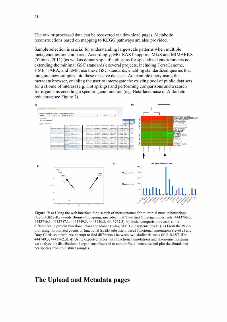
(Yilmaz, 2011) (as well as domain-specific plug-ins for specialized environments not extending the minimal GSC standards); several projects, including TerraGenome, HMP, TARA, and EMP, use these GSC standards, enabling standardized queries that integrate new samples into these massive datasets. An example query using the metadata browser, enabling the user to interrogate the existing pool of public data sets for a Biome of interest (e.g. Hot springs) and performing comparisons and a search for organisms encoding a specific gene function (e.g. Beta-lactamase or Aldo/keto reductase; see Figure 7).  

 Figure 7: a) Using the web interface for a search of metagenomes for microbial mats in hotsprings (GSC-MIMS-Keywords Biome=”hotspring; microbial mat”) we find 6 metagenomes (refs: 4443745.3, 4443746.3, 4443747.3, 4443749.3, 4443750.3, 4443762.3). b) Initial comparison reveals some differences in protein functional class abundance (using SEED subsystems level 1). c) From the PCoA plot using normalized counts of functional SEED subsystem based functional annotations (level 2) and Bray-Curtis as metric, we attempt to find differences between two similar datasets (MG-RAST-IDs: 444749.3, 4443762.3). d) Using exported tables with functional annotations and taxonomic mapping we analyze the distribution of organisms observed to contain Beta-lactamase and plot the abundance per species from to distinct samples..  

 

 

The Upload and Metadata pages  

11  

 

Data and Metadata can be uploaded in the form of spreadsheets along with the sequence data using both the ftp and the http protocols. The web uploader will automatically split larger files and allow parallel uploads.  

MG-RAST supports datasets that are augmented with rich metadata using the standards and technology developed by the GSC.  

Each user has a temporary storage location inside the MG-RAST system. This “inbox” provides temporary storage for data and metadata to be submitted to the system. Using the inbox users can extract compressed files, convert a number of vendor specific formats to MG-RAST submission compliant formats and obtain an MD5 checksum for verifying that transmission to MG-RAST has not altered the data.  

The web uploader has been optimized for large data sets of over 100GBp (gigabasepairs) often resulting in file sizes in excess of 150 GB.  

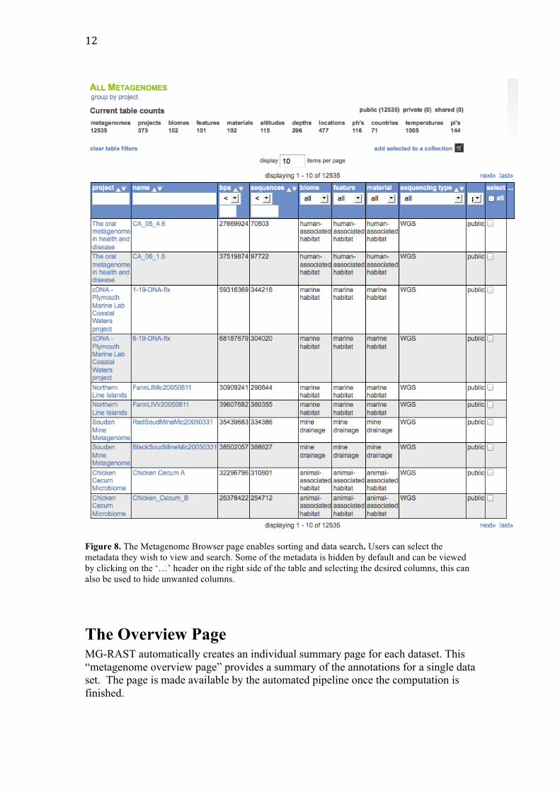
Metadata enabled data discovery  The Metagenome Browse page list all data sets visible to the user. Datasets in MG-RAST are private by default, but the submitting user has the option to share datasets with specific users or to make datasets public. This page also provides an overview of the non-public data sets submitted by the user or shared with them. Figure 8 shows the metagenome browse table, which provides an interactive graphical means to discover data based on technical data (e.g. sequence type or data set size) or metadata (e.g. location or biome).  

12  

 

 Figure 8. The Metagenome Browser page enables sorting and data search. Users can select the metadata they wish to view and search. Some of the metadata is hidden by default and can be viewed by clicking on the ‘…’ header on the right side of the table and selecting the desired columns, this can also be used to hide unwanted columns.  

 

The Overview Page  MG-RAST automatically creates an individual summary page for each dataset. This “metagenome overview page” provides a summary of the annotations for a single data set. The page is made available by the automated pipeline once the computation is finished.  

13  

 

The page is intended as a single point of reference for metadata, quality and data. It also provides an initial overview of the analysis results for individual data sets with default parameters. Further analysis are available on the Analysis page.  

 

Technical detail on the overview page  The Overview page provides the MG-RAST ID for a data set, a unique identifier that is usable as accession number for publications. Additional information like the Name of the submitting PI and organization and a user provided metagenome name are displayed at the top of the page as well. A static URL for linking to the system that will be stable across changes to the MG-RAST web interface is provided as additional information (Figure 9).  

 Figure 9: Top of the metagenome overview page.  

We provide an automatically generated paragraph of text describing the submitted data and the results computed by the pipeline. Via the project information we display additional information provided by the data submitters at the time of submission or later.  

 Figure 10: Sequences to the pipeline are classified into one of 5 categories. grey = failed the QC, red = unknown sequences, yellow = unknown function but protein coding, green = protein coding with known function and blue = ribosomal RNA. For this example just under 20% of the sequences were either filtered by QC or failed to be recognized as either protein coding or ribosomal.  

One of the key diagrams in MG-RAST is the sequence breakdown pie chart (Figure 10) classifying the submitted sequences submitted into several categories according to

14  

 

their annotation status. As detailed in the description of the MG-RAST v3 pipeline above, the features annotated in MG-RAST are protein coding genes and ribosomal proteins.  

It should be noted that for performance reasons no other sequence features are annotated by the default pipeline. Other feature types e.g. small RNAs or regulatory motifs (e.g. CRISPRS (Bolotin, Quinquis, Sorokin & Ehrlich, 2005)) will not only require significantly higher computational resources but also are frequently not supported by the unassembled short reads that comprise the vast majority of today’s metagenomic data in MG-RAST.  

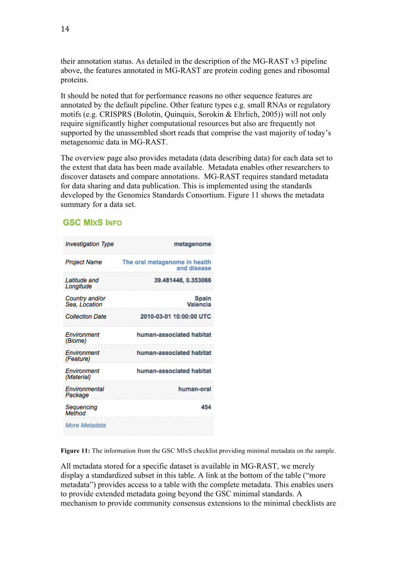
The overview page also provides metadata (data describing data) for each data set to the extent that data has been made available. Metadata enables other researchers to discover datasets and compare annotations. MG-RAST requires standard metadata for data sharing and data publication. This is implemented using the standards developed by the Genomics Standards Consortium. Figure 11 shows the metadata summary for a data set.  

 Figure 11: The information from the GSC MIxS checklist providing minimal metadata on the sample.  

All metadata stored for a specific dataset is available in MG-RAST, we merely display a standardized subset in this table. A link at the bottom of the table (“more metadata”) provides access to a table with the complete metadata. This enables users to provide extended metadata going beyond the GSC minimal standards. A mechanism to provide community consensus extensions to the minimal checklists are

15  

 

the environmental packages are explicitly encouraged, but not required when using MG-RAST.  

Metagenome  QC  The analysis flowchart and analysis statistics provide an overview of the number of sequences at each stage in the pipeline. (Figure 12). The text block next to the analysis flowchart presents the numbers next to their definitions.  

 Figure 12. The analysis flowchart provides an overview of the fractions of sequences “surviving” the various steps of the automated analysis. In this case about 44% of sequences were filtered during quality control. From the remaining 66,764,893 sequences, 58.9% were predicted to be protein coding and 10.4% hit ribosomal RNA. From the predicted proteins, 79.8% could be annotated with a putative protein function. Out of 55,748,499 annotated proteins, 44,493,781 have been assigned to a functional classification (SEED, COG, eggNOG, KEGG).  

Technical  Data  This part provides a quick links to a general statistical overview of the different analysis steps performed (see Analysis flowchart), a comprehensive list of all metadata for the data set, sequence length and GC distributions and a breakdown of blat hits per data source (e.g. hits to RefSeq (Pruitt, Tatusova & Maglott, 2007) , UniProt (UniProt Consortium, 2013) or SEED (Overbeek et al., 2005)).  

The Analysis Statistics and Analysis Flowchart provide sequence statistics for the main steps in the pipeline from raw data to annotation, describing the transformation of the data between steps.  

Sequence length and GC histograms display the distribution before and after quality control steps.  

Metadata is presented in a searchable table which contains contextual metadata describing sample location, acquisition, library construction and sequencing using GSC compliant metadata. All metadata can be downloaded from the table.  

16  

 

 

Taxonomic and functional information on the overview page    

Organism Breakdown  The taxonomic hit distribution display breaks down taxonomic units into a series of pie charts of all the annotations grouped at various taxonomic ranks (Domain, Phylum, Class, Order, Family, Genus). The subsets are selectable for downstream analysis, this also enables downloads of subsets of reads, e.g. those hitting a specific taxonomic unit.  

The  rank  abundance  plot  (Figure  13)  provides  a  rank-­‐ordered  list  of  taxonomic  units  at  a  user-­‐defined  taxonomic  level,  ordered  by  their  abundance  in  the  annotations.    

  Figure 13: Rank abundance plot by phylum.  

The rarefaction curve of annotated species richness is a plot of the total number of distinct species annotations as a function of the number of sequences sampled. The slope of the right-hand part of the curve is related to the fraction of sampled species that are rare. When the rarefaction curve is flat, more intensive sampling is likely to yield only few additional species. The rarefaction curve is derived from the protein taxonomic annotations and is subject to problems stemming from technical artifacts. These artifacts can be similar to the ones affecting amplicon sequencing (Reeder & Knight 2009) but the process of inferring species from protein similarities may introduce additional uncertainty.  

Finally in this section we display an estimate of the alpha diversity based on the taxonomic annotations for the predicted proteins. The alpha diversity is presented in context of other metagenomes in the same project.  

17  

 

Functional Breakdown  This section contains four pie charts providing a breakdown of the functional categories for KEGG (Kanehisa et al., 2012), COG (Vasudevan et al., 2003), SEED Subsystems (overbeek et al., 2005) and EggNOGs (Jensen et al., 2008). Clicking on the individual pie chart slices will save the respective sequences to the workbench.  

The relative abundance of sequences per functional category can be downloaded as a spreadsheet and users can browse the functional breakdowns via the Krona tool (Onodov, Bergman & Phillippy, 2011) integrated in the page.  

A more detailed functional analysis, allowing the user to manipulate parameters for sequence similarity matches is available via the analysis page.  

 

The  Analysis  Page  The MG-RAST annotation pipeline produces a set of annotations for each sample; these annotations can be interpreted as functional or taxonomic abundance profiles. The analysis page can be used to view these profiles for a single metagenome, or compare profiles from multiple metagenomes using various visualizations (e.g. heatmap) and statistics (e.g. PCoA , normalization).  

The page breaks down in three parts following a typical workflow (Figure 14):  

1. Selection of an MG-RAST analysis scheme, that is selection of a particular taxonomic or functional abundance profile mapping. For taxonomic annotations, since there is not always a unique mapping from hit to annotation, we provide three interpretations: Best Hit, Representative Hit and Lowest Common Ancestor as explained below. Functional annotations can either be grouped into mappings to functional hierarchies or displayed without a hierarchy. In addition the recruitment plot displays the recruitment of protein sequences against a reference genome.  

2. Selection of sample and parameters. This dialog allows the selection of multiple metagenomes which can be compared undividually, or selected and compared as groups. Comparison is always relative to the annotation source, e-value and percent identity cutoffs selectable in this section. In addition to the metagenomes available in MG-RAST, sets of sequences previously saved in the workbench can be selected for visualization.  

3. Data Visualization and Comparison. Depending on the selected profile type, the profiles for the metagenomes can be visualized and compared using “barcharts”, “trees”, spreadsheet like “tables” , “heatmaps”, “PCoA”, “rarefaction plots”, “Circular recruitment plot” and KEGG maps.  

18  

 

 Figure 14: Using the analysis page is a three step process. First select a profile and hit (see below) type. Second select a list of metagenomes and set annotation source and similarity parameters. Third chose a comparison.  

 

Representative hit, best hit, and Lowest Common Ancestor interpretation  MG-RAST searches the non-redundant M5NR and M5RNA databases in which each sequence is unique. These two databases are built from multiple sequence database sources and the individual sequences may occur multiple times in different strains and species (and sometimes genera) with 100% identity. In these circumstances, choosing the “right” taxonomic information is not a straightforward process.  

To optimally serve a number of different use cases, we have implemented three different ways of finding the “right” function or taxon information. This impacts the end-user experience as they have three different methods to choose the number of hits reported for a given sequence in their data set. The details on the three different classification functions implemented are below:  

Best Hit  

The best hit classification reports the functional and taxonomic annotation of the best hit in the M5NR for each feature. In those cases where the similarity search yields multiple same-scoring hits for a feature, we do not choose any single “correct” label. For this reason we have decided to “double count” all annotations with identical match properties and leave determination of truth to our users. While this approach aims to inform about the functional and taxonomic potential of a microbial community by preserving all information, subsequent analysis can be biased because of a single feature having multiple annotations, leading to inflated hit counts. If you are looking for a specific species or function in your results, the “best hit” function is likely what you are looking for.  

Representative Hit  

The representative hit classification selects a single unambiguous annotation for each feature. The annotation is based on the first hit in the homology search and the first annotation for that hit in our database. This makes counts additive across functional

19  

 

and taxonomic levels and thus allows for example to compare functional and taxonomic profiles of different metagenomes.  

Lowest Common Ancestor (LCA)  

To avoid the problem of multiple taxonomic annotations for a single feature we provide taxonomic annotations based on the widely used LCA-method (lowest common ancestor) introduced by MEGAN (Huson, Auch, Qi & Schuster, 2007). In this method all hits that have a bit score close to the bit score of the best hit are collected. The taxonomic annotation of the feature is then determined by computing the LCA of all species in this set. This replaces all taxonomic annotations from ambiguous hits with a single higher level annotation in the NCBI taxonomy tree.  

The number of hits (“occurrences of the input sequence in the database”) may be inflated if the “best hit” filter is used, or your favorite species might be missing despite a very similar sequence similarity result if using the “representative hit” classifier function (in fact 100% identical match to your favorite species exists).  

One way to consider both “representative” and “best” hit is that they over-interpret the available evidence, with the LCA classifier function any input sequence is only classified down to a trustworthy taxonomic level. While naively this seems to be the best function to choose in all cases as it classifies sequences to varying depths, this causes problems for downstream analysis tools that might rely on everything being classified to the same level.  

Normalization  Normalization  refers  to  a  transformation  that  attempts  to  reshape  an  underlying  distribution.      A  large  number  of  biological  variables  exhibit  a  log-­‐normal  distribution,  meaning  that  when  you  transform  the  data  with  a  log  transformation,  the  values  exhibit  a  normal  distribution.      Log-­‐transformation  of  the  counts  data  makes  a  normalized  data  product  that  is  more  likely  to  satisfy  the  assumptions  additional  downstream  tests  like  ANOVA  or  t-­‐tests.    

Standardization  is  a  transformation  applied  to  each  distribution  in  a  group  of  distributions  so  that  all  distributions  exhibit  the  same  mean  and  the  same  standard  deviation.  This  removes  some  aspects  of  inter-­‐sample  variability  and  can  make  data  more  comparable.  This  sort  of  procedure  is  analogous  to  commonly  practiced  scaling  procedures,  but  is  more  robust  in  that  it  controls  for  both  scale  and  location.    

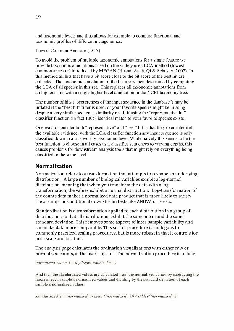
The  analysis  page  calculates  the  ordination  visualizations  with  either  raw  or  normalized  counts,  at  the  user’s  option.    The  normalization  procedure  is  to  take    

normalized_value_i = log2(raw_counts_i + 1)  

And then the standardized values are calculated from the normalized values by subtracting the mean of each sample’s normalized values and dividing by the standard deviation of each sample’s normalized values.  

standardized_i = (normalized_i - mean({normalized_i})) / stddev({normalized_i})  

20  

 

You can read more about these procedures in a number of texts - We recommend Terry Speed’s “Statistical Analysis of Gene Expression in Microarray Data” (ISBN1584883278).  

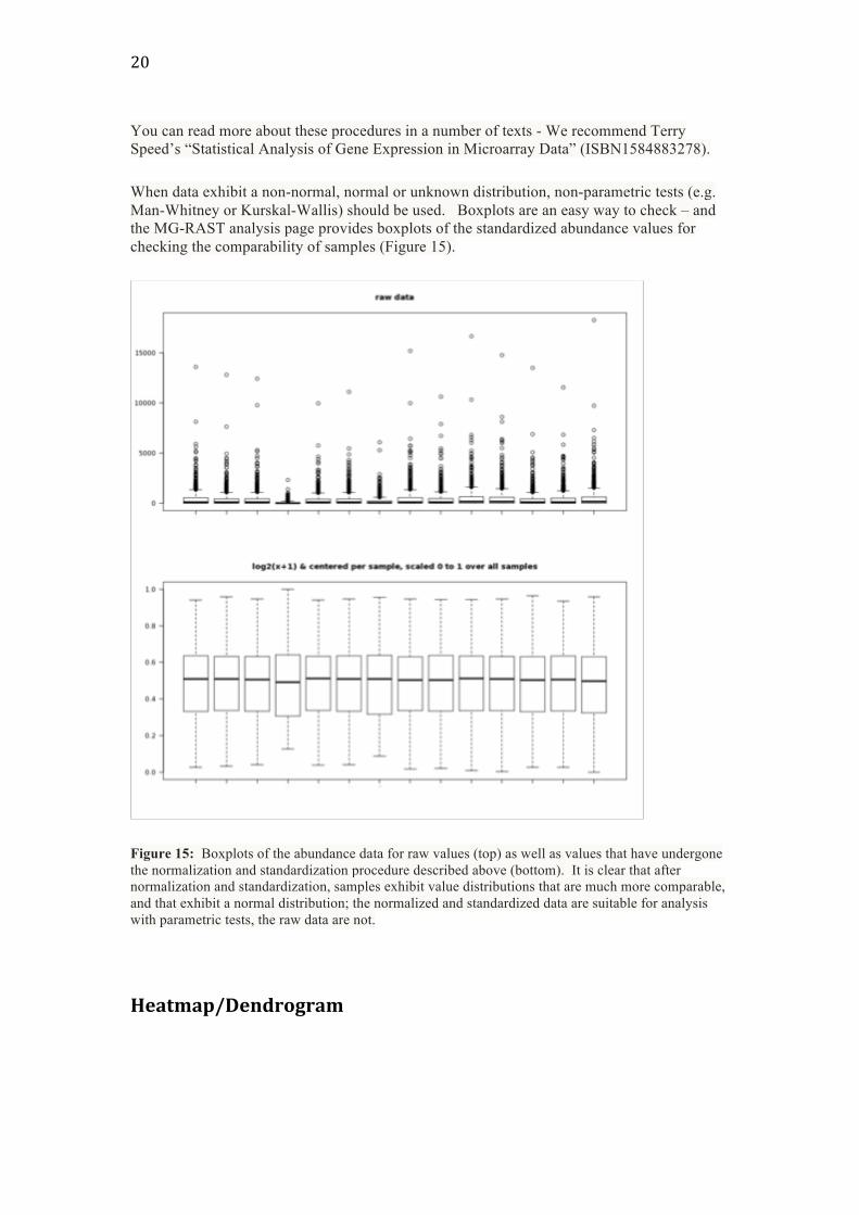
When data exhibit a non-normal, normal or unknown distribution, non-parametric tests (e.g. Man-Whitney or Kurskal-Wallis) should be used. Boxplots are an easy way to check – and the MG-RAST analysis page provides boxplots of the standardized abundance values for checking the comparability of samples (Figure 15).  

 

Figure 15: Boxplots of the abundance data for raw values (top) as well as values that have undergone the normalization and standardization procedure described above (bottom). It is clear that after normalization and standardization, samples exhibit value distributions that are much more comparable, and that exhibit a normal distribution; the normalized and standardized data are suitable for analysis with parametric tests, the raw data are not.  

 

Heatmap/Dendrogram    

21  

 

 Figure 16: Heatmap/dendogram example in MG-RAST. The MG-RAST heatmap/dendrogram has two dendrograms, one indicating the similarity/dissimilarity among metagenomic samples (x axis dendrogram) and another to indicate the similarity/dissimilarity among annotation categories (e.g., functional roles; the y-axis dendrogram).      The heatmap/dendrogram (Figure 16) is a tool that allows an enormous amount of information to be presented in a visual form that is amenable to human interpretation. Dendrograms are trees that indicate similarities between annotation vectors. The MG-RAST heatmap/dendrogram has two dendrograms, one indicating the similarity/dissimilarity among metagenomic samples (x axis dendrogram) and another to indicate the similarity/dissimilarity among annotation categories (e.g., functional roles; the y-axis dendrogram). A distance metric is evaluated between every possible pair of sample abundance profiles. A clustering algorithm (e.g ward-based clustering) then produces the dendrogram trees. Each square in the heatmap dendrogram represents the abundance level of a single category in a single sample. The values used to generate the heatmap/dendrogram figure can be downloaded as a table by clicking on the “download” button.  

 

Barchart  and  tree  The barchart and tree tools map raw or normalized abundances onto functional or taxonomic hierarchies. The barchart tool presents mapping onto the highest category of a hierarchy (e.g. Domain) and allows a drill down into the hierarchy. In addition reads from a specific level can be added into the workbench.  

Ordination  MG-RAST uses Principle Coordinate Analysis (PCoA) to reduce the dimensionality of comparisons of multiple samples that consider functional or taxonomic annotations.  

PCoA is a well known method for dimensionality reduction of large data sets. Dimensionality reduction is a process that allows the complex variation found in a

22  

 

large data sets (e.g. the abundance values of thousands of functional roles or annotated species across dozens of metagenomic samples) to be reduced to a much smaller number of variables that can be visualized as simple 2 or 3 dimensional scatter plots. The plots enable interpretation of the multidimensional data in a human-friendly presentation. Samples that exhibit similar abundance profiles (taxonomic or functional) group together, whereas those that differ are found further apart. A key feature of PCoA based analyses is that users can compare components not just to each other, but to metadata recorded variables (e.g. sample pH, biome, DNA extraction protocol etc.) to reveal correlations between extracted variation and metadata-defined characteristics of the samples. It is also possible to couple PCoA with higher resolution statistical methods to identify individual sample features (taxa or functions) that drive correlations observed in PCoA visualizations. This can be accomplished with permutation based statistics applied directly to the data before calculation of distance measures used to produce PCoAs, or by applying conventional statistical approaches (e.g. ANOVA or Kruskal-Wallis test) to groups observed in PCoA based visualizations.  

Table  The table tool creates a spreadsheet based abundance table that can be searched and restricted by the user. Tables can be generated at user-selected levels of phylogenetic or functional resolution. Table data can be visualized using Krona (Ondov 2011), can be exported in BIOM format to be used in other tools, e.g. QIIME (Caporaso et al., 2010), or the tables can be exported as tab-separated text. Abundance tables serve as the basis for all comparative analysis tools in MG-RAST, from PCoA to heatmap-dendrograms.  

KEGG maps  The KEGG map tool allows the visual comparison of predicted metabolic pathways in metagenomic samples. It maps the abundance of identified enzymes onto a KEGG (Kanehisa et al., 2012) map of functional pathways. Metagenomes can be assigned into one of two groups and those groups can be visually compared.  

 

4. How to drill down using the workbench  One of the new features of MGRAST v3 is the workbench. It is the main mechanism for exchanging subsets of data between analysis views. It also allows you to download the FASTA files of a selection of proteins.  

When you initially go to the analysis page, your workbench will be empty. It is displayed as the leftmost tab in the data tabular view. So how do you get data into the workbench? There are two simple ways to select data subsets – from any generated table or from the drilldown of a barchart.  

23  

 

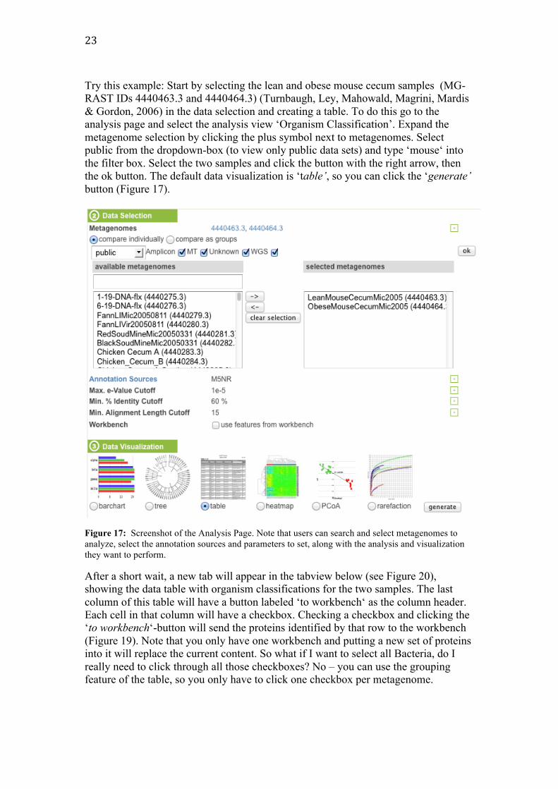
Try this example: Start by selecting the lean and obese mouse cecum samples (MG-RAST IDs 4440463.3 and 4440464.3) (Turnbaugh, Ley, Mahowald, Magrini, Mardis & Gordon, 2006) in the data selection and creating a table. To do this go to the analysis page and select the analysis view ‘Organism Classification’. Expand the metagenome selection by clicking the plus symbol next to metagenomes. Select public from the dropdown-box (to view only public data sets) and type ‘mouse‘ into the filter box. Select the two samples and click the button with the right arrow, then the ok button. The default data visualization is ‘table’, so you can click the ‘generate’ button (Figure 17).  

 Figure 17: Screenshot of the Analysis Page. Note that users can search and select metagenomes to analyze, select the annotation sources and parameters to set, along with the analysis and visualization they want to perform.  

After a short wait, a new tab will appear in the tabview below (see Figure 20), showing the data table with organism classifications for the two samples. The last column of this table will have a button labeled ‘to workbench‘ as the column header. Each cell in that column will have a checkbox. Checking a checkbox and clicking the ‘to workbench‘-button will send the proteins identified by that row to the workbench (Figure 19). Note that you only have one workbench and putting a new set of proteins into it will replace the current content. So what if I want to select all Bacteria, do I really need to click through all those checkboxes? No – you can use the grouping feature of the table, so you only have to click one checkbox per metagenome.  

24  

 

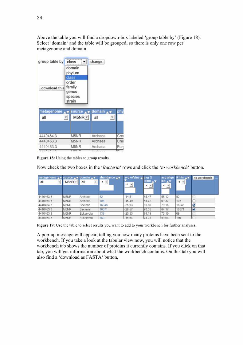
Above the table you will find a dropdown-box labeled ‘group table by’ (Figure 18). Select ‘domain‘ and the table will be grouped, so there is only one row per metagenome and domain.  

 Figure 18: Using the tables to group results.  

Now check the two boxes in the ‘Bacteria‘ rows and click the ‘to workbench‘ button.  

 Figure 19: Use the table to select results you want to add to your workbench for further analyses.  

A pop-up message will appear, telling you how many proteins have been sent to the workbench. If you take a look at the tabular view now, you will notice that the workbench tab shows the number of proteins it currently contains. If you click on that tab, you will get information about what the workbench contains. On this tab you will also find a ‘download as FASTA‘ button,  

 

 

25  

 

 Figure 20: View of the workbench with the summary of the proteins that have been added.  

Aside from being able to download the sequences of your selected proteins, you can also use them to generate other visualizations. This includes switching from organism to functional classification. To to this, simply check the ‘use proteins from workbench‘ checkbox in the data selection when generating a new visualization, e.g. a circular tree using the proteins we just buffered.  

The table is not the only visualization that allows to put a subselection into the workbench. You can also use the barchart to do this (Figure 21). Simply click on the ‘to workbench’ button next to the headline of a drilldown. Note that you cannot put the topmost barchart into the workbench, as it is not yet a subselection of proteins.  

 

 Figure 21: In addition to the results table, users can download results or add to their workbench from barcharts.  

 

2.6 Downloads  

26  

 

The workbench feature stores sub-selections of data and allows those to be used as input for further selection or displays, e.g. select all E. coli reads and then display the functional categories present just in E. coli reads across multiple data sets. In addition the workbench allows downloading the annotated reads for the sub-selection stored in the workbench as fasta (Figure 22).  

 Figure 22: The workbench facilitates the download of selected reads using the name space of the selection.  

Once processing data sets in MG-RAST is finished a download page is created for the project. On this page all data products created during the computation are made available as files. In addition, datasets which have been published in MG-RAST have links to an ftp site at the top of this page where you can download additional information.  

 

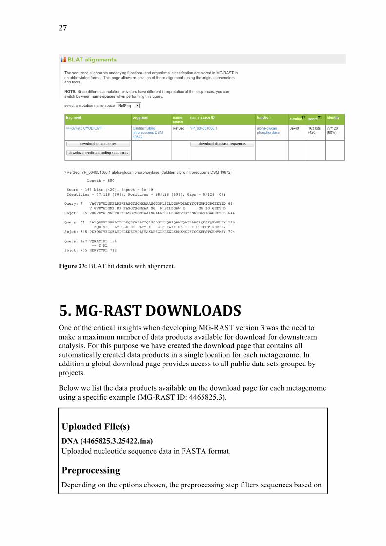
Viewing Evidence  For  individual  proteins,  the  MG-­‐RAST  page  allows  users  to  retrieve  the  sequence  alignments  underlying  the  annotation  transfers  (see  Figure  23).  Using  the  M5NR  (Wilke,  2011)  technology  users  can  retrieve  alignments  against  the  database  of  interest  with  no  additional  overhead.  

27  

 

 Figure 23: BLAT hit details with alignment.  

 

5.  MG-­‐RAST  DOWNLOADS  One of the critical insights when developing MG-RAST version 3 was the need to make a maximum number of data products available for download for downstream analysis. For this purpose we have created the download page that contains all automatically created data products in a single location for each metagenome. In addition a global download page provides access to all public data sets grouped by projects.  

Below we list the data products available on the download page for each metagenome using a specific example (MG-RAST ID: 4465825.3).  

Uploaded File(s)  DNA (4465825.3.25422.fna)  Uploaded nucleotide sequence data in FASTA format.  

Preprocessing  Depending on the options chosen, the preprocessing step filters sequences based on

28  

 

length, number of ambiguous bases and quality values if available.  passed, DNA (4465825.3.100.preprocess.passed.fna)  

A FASTA formatted file containing the sequences which were accepted and will be passed on to the next stage of the analysis pipeline.  

removed, DNA (4465825.3.100.preprocess.removed.fna)  

A FASTA formatted file containing the sequences which were rejected and will not be passed on to the next stage of the analysis pipeline.  

Dereplication  The optional dereplication step removes redundant “technical replicate” sequences from the metagenomic sample. Technical replicates are identified by binning reads with identical first 50 base-pairs. One copy of each 50-base-pair identical bin is retained.  passed, DNA (4465825.3.150.dereplication.passed.fna)  

A FASTA formatted file containing one sequence from each bin which will be passed on to the next stage of the analysis pipeline.  

removed, DNA (4465825.3.150.dereplication.removed.fna)  

A FASTA formatted file containing the sequences which were identified as technical replicates and will not be passed on to the next stage of the analysis pipeline.  

Screening  The optional screening step screens reads against model organisms using bowtie to remove reads which are similar to the genome of the selected species.  passed, DNA (4465825.3.299.screen.passed.fna)  

A FASTA formatted file containing the reads which which had no similarity to the selected genome and will be passed on to the next stage of the analysis pipeline.  

Prediction of protein coding sequences  Coding regions within the sequences are predicted using FragGeneScan, an ab-initio prokaryotic gene calling algorithm. Using a hidden Markov model for coding regions and non-coding regions, this step identifies the most likely reading frame and translates nucleotide sequences into amino acids sequences. The predicted coding regions, possibly more than one per fragment, are called features.  coding, Protein (4465825.3.350.genecalling.coding.faa)  

A amino-acid sequence FASTA formatted file containing the translations of the predicted coding regions.  

29  

 

coding, DNA (4465825.3.350.genecalling.coding.fna)  

A nucleotide sequence FASTA formatted file containing the predicted coding regions.  

RNA Clustering  Sequences from step 2 (before dereplication) are pre-screened for at least 60% identity to ribosomal sequences and then clustered at 97% identity using UCLUST. These clusters are checked for similarity against the ribosomal RNA databases (Greengenes, LSU, SSU, and RDP).  rna97, DNA (4465825.3.440.cluster.rna97.fna)  

A FASTA formatted file containing sequences that have at least 60% identity to ribosomal sequences and are checked for RNA similarity.  

rna97, Cluster (4465825.3.440.cluster.rna97.mapping)  

A tab-delimited file that identifies the sequence clusters and the sequences that comprise them.  

The columns making up each line in this file are:  

1 Cluster ID, e.g. rna97_998  2 Representative read ID, e.g. 11909294  3 List of IDs for other reads in the cluster, e.g. 11898451,11944918  4 List of percentage identities to the representative read sequence, e.g.

97.5%,100.0%  

RNA similarities  The two files labelled ‘expand’ are comma- and semicolon- delimited files that provide the mappings from md5s to function and md5s to taxonomy:  annotated, Sims (4465825.3.450.rna.expand.lca)  

annotated, Sims (4465825.3.450.rna.expand.rna)  

Packaged results of the blat search against all the DNA databases with md5 value of the database sequence hit followed by sequence or cluster ID, similarity information, annotation, organism, database name.  

raw, Sims (4465825.3.450.rna.sims)  

This is the similarity output from BLAT. This includes the identifier for the query which is either the FASTA id or the cluster ID, and the internal identifier for the sequence that it hits.  

The fields are in BLAST m8 format:  

1 Query id (either fasta ID or cluster ID), e.g. 11847922  

30  

 

2 Hit id, e.g. lcl|501336051b4d5d412fb84afe8b7fdd87  3 percentage identity, e.g. 100.00  4 alignment length, e.g. 107  5 number of mismatches, e.g. 0  6 number of gap openings, e.g. 0  7 q.start, e.g. 1  8 q.end, e.g. 107  9 s.start, e.g. 1262  10 s.end, e.g. 1156  11 e-value, e.g. 1.7e-54  12 score in bits, e.g. 210.0  

 filtered, Sims (15:04 4465825.3.450.rna.sims.filter)  This is a filtered version of the raw Sims file above that removes all but the best hit for each data source.  

Gene Clustering  Protein coding sequences are clustered at 80% identity with UCLUST. This process does not remove any sequences but instead makes the similarity search step easier. Following the search, the original reads are loaded into MG-RAST for retrieval on-demand.    

aa90, Protein (4465825.3.550.cluster.aa90.faa)  

An amino acid sequence FASTA formatted file containing the translations of one sequence from each cluster (by cluster ids starting with aa90_) and all the unclustered (singleton) sequences with the original sequence ID.  

aa90, Cluster (4465825.3.550.cluster.aa90.mapping)  

A tab-separated file in which each line describes a single cluster.  

The fields are:  

1 Cluster ID, e.g. aa90_3270  2 protein coding sequence ID including hit location and strand, e.g.

11954908_1_121_+  3 additional sequence ids including hit location and strand, e.g.

11898451_1_119_+,11944918_19_121_+  4 sequence % identities, e.g. 94.9%,97.0%  

Protein similarities  annotated, Sims (4465825.3.650.superblat.expand.lca)  The expand.lca file decodes the md5 to the taxonomic classification it is annotated

31  

 

with.  

The format is:  

1 md5(s), e.g. cf036dfa9cdde3a8a4c09d7fabfd9ba5;1e538305b8319dab322b8f28da82e0a1  

2 feature id (for singletons) or cluster id of hit including hit location and strand, e.g. 11857921_1_101_-  

3 alignment %, e.g. 70.97;70.97  4 alignment length, e.g. 31;31  5 E-value, e.g. 7.5e-05;7.5e-05  6 Taxonomic string, e.g. Bacteria;Actinobacteria;Actinobacteria

(class);Coriobacteriales;Coriobacteriaceae;Slackia;Slackia exigua;-    annotated, Sims (4465825.3.650.superblat.expand.protein)  Packaged results of the blat search against all the protein databases with md5 value of the database sequence hit followed by sequence or cluster ID, similarity information, functional annotation, organism, database name.  

Format is:  

1 md5 (identifier for the database hit), e.g. 88848aa7224ca2f3ac117e7953edd2d9  

2 feature id (for singletons) or cluster ID for the query, e.g. aa90_22837  3 alignment % identity, e.g. 76.47  4 alignment length, e.g. 34  5 E-value, e.g. 1.3e-06  6 protein functional label, e.g. SsrA-binding protein  7 Species name associated with best protein hit, e.g. Prevotella bergensis

DSM 17361 RefSeq 585502    raw, Sims (4465825.3.650.superblat.sims)  Blat output with sequence or cluster ID, md5 value for the sequence in the database and similarity information.  

filtered, Sims (4465825.3.650.superblat.sims.filter)  

Blat output filtered to take only the best hit from each data source.  

 

6. DISCUSSION  We have described MG-RAST, a community resource for the analysis of metagenomic sequence data. We have developed a new pipeline and environment for automated analysis of shotgun metagenomic data, as well as a series of interactive

32  

 

tools for comparative analysis. The pipeline is also being used for the analysis of metatranscriptome data as well as amplicon data of various kinds. This service is being used by thousands of users worldwide, many contributing their data and analysis results to the community. We believe that community resources, such as MG-RAST, will fill a vital role in the bioinformatics ecosystem in the years to come.  

 

MG-RAST has become a community clearinghouse for metagenomic data and analysis, with over 12,000 public data sets that can be freely used. Because analysis was performed in a uniform way, these data sets can be used as building blocks for new comparative analysis; so long as new data sets are analyzed similarly, results are robustly comparable between new and old data set analysis. These data sets (and the resulting analysis data products) are made available for download and reuse as well.  

Community resources like MG-RAST provide an interesting value proposition to the metagenomics community: First, it enables low-cost meta-analysis. Users utilize the data products in MG-RAST as a basis for comparison without the need to re-analyze every data set used in their studies. The high computational cost of analysis (Wilkening, Wilke, Desai & Meyer, 2009) cite Wilkening) makes pre-computation a prerequisite for large scale meta-analyses. In 2001, Angiuli et al., determined the real currency cost of re-analysis for the over 12,000 data sets openly available on MG-RAST to be in excess of 30 million US-dollars if Amazon’s EC2 platform is used (Angiuoli, Matalka, Gussman, Galens, Vangala, Riley, et al. 2011). This figure doesn’t consider the 66,000 private data sets that have been analyzed with MG-RAST.  

Second, it provides incentives to the community to adopt standards, both in terms of metadata and analysis approaches. Without this standardization, data products aren’t readily reusable, and computational costs quickly become unsustainable. We are not arguing that a single analysis is necessarily suitable for all users, rather, we are pointing out that if one particular type of analysis is run for all data sets, the results can be efficiently reused, amortizing costs. Open access to data and analyses foster community interactions that make it easier for researchers’ efforts to achieve consensus with respect to establishing best practises as well as identifying methods and analyses that could provide misleading results.  

Third, community resources drive increased efficiency and computational performance. Community resources consolidate the demand for analysis resources sufficiently to drive innovation in algorithms and approaches. Due to this demand, the MG-RAST team has needed to scale the efficiency of their pipeline by a factor of nearly 1000 over the last four years. This drive has caused improvements in gene calling, clustering, sequence quality analysis, as well as many other areas. In less specialized groups with less extreme computational needs, this sort of efficiency gain would be difficult to achieve. Moreover, the large quantities of data sets that flow through the system have forced the hardening of the pipeline against a large variety of sequence pathology types that wouldn’t be readily observed in smaller systems.  

We believe that our experiences in the design and operation of MG-RAST are representative of bioinformatics as a whole. The community resource model is critical if we are to benefit from the exponential growth in sequence data. This data has the potential to enable new insights into the world around us, but only if we can analyze it

33  

 

effectively. It is only due to this approach that we have been able to scale to the demands of our users effectively, analyzing over 200 billion sequences thus far.  

We note that scaling to the required throughput by adding hardware to the system or simply renting time using an unoptimized pipeline on e.g. Amazon’s EC2 machine would not be economically feasible. The real currency cost on EC2 for the data currently analyzed in MG-RAST (26 Terabasepairs) would be in excess of 100 million US dollars using an unoptimized workflow like CLOVR (Angiuoli et al., 2011).  

 

All of MG-RAST is open source and available on https://github.com/MG-RAST  

7. FUTURE WORK  While MG-RAST v3 is a substantial improvement over prior systems, much work remains to be done. Data set sizes continue to increase at an exponential pace. Keeping up with this change remains a top priority, as metagenomics users continue to benefit from increased resolution of microbial communities. Upcoming versions of MG-RAST will include: (1) mechanisms for speeding pipeline up using data reduction strategies that are biologically motivated; (2) opening up the data ecosystem via an API that will enable third-party development and enhancements; (3) providing distributed compute capabilities using user-provided resources; as well as (4) providing virtual integration of local data sets to allow comparison between local data and shared data without requiring full integration.  

8. References  Angiuoli, S.V., Matalka, M., Gussman, A., Galens, K., Vangala, M., Riley, D.R., et al. (2011). CloVR: a virtual machine for automated and portable sequence analysis from the desktop using cloud computing. BMC Bioinformatics, 12:356.  

Benson, D.A., Cavanaugh, M., Clark, K., Karsch-Mizrachi, I., Lipman, D.J., Ostell, J., et al. (2012). GenBank. Nucleic Acids Res. 41(Database issue):D36-42.  

Bolotin, A., Quinquis, B., Sorokin, A., & Ehrlich, S.D. (2005). Clustered regularly interspaced short palindrome repeats (CRISPRs) have spacers of extrachromosomal origin. Microbiology. 151(Pt 8):2551-61.  

Caporaso, J.G., Kuczynski, J., Stombaugh, J., Bittinger, K., Bushman, F.D., Costello, E.K., et al. (2010). QIIME allows analysis of high-throughput community sequencing data. Nature Methods, 7(5):335-6.  

Cox, M.P., Peterson, D.A., Biggs, P.J., & Solexa, Q.A. (2010). At-a-glance quality assessment of Illumina second-generation sequencing data. BMC Bioinformatics, 11:485.  

34  

 

Edgar, R.C. (2010). Search and clustering orders of magnitude faster than BLAST. Bioinformatics, 26: 2460–2461  

Field D, Amaral-Zettler L, Cochrane G, Cole JR, Dawyndt P, Garrity GM, et al. (2011). The Genomic Standards Consortium. PLoS Biol., 9(6).  

Gabriel, E., Fagg, G.E., Bosilca, G., Angskun, T., Dongarra, J.J.,. Squyres, J.M., et al. (2004). In Proceedings, 11th European PVM/MPI Users' Group Meeting.  

Gene Ontology Consortium. (2013). Gene Ontology annotations and resources. Nucleic Acids Res., 41(Database issue):D530-5.  

Gomez-Alvarez, V., Teal, T. K. & Schmidt, T. M. (2009). Systematic artifacts in metagenomes from complex microbial communities. ISME J., 3, 1314-1317.  

Huse, S.M,, Huber, J.A., Morrison, H.G., Sogin, M.L., & Welch, D.M. (2007). Accuracy and quality of massively parallel DNA pyrosequencing. Genome Biol., 8(7):R143.  

Huson, D.H., Auch, A.F., Qi, J., & Schuster, S.C. (2007). MEGAN analysis of metagenomic data. Genome Research, 17, 377-386.  

Jensen, L.J., Julien, P., Kuhn, M., von Mering, C., Muller, J., Doerks, T., & Bork, P. (2008). eggNOG: automated construction and annotation of orthologous groups of genes. Nucleic Acids Res., 36(Database issue):D250-4.  

Kanehisa, M., Goto, S., Sato, Y., Furumichi, M., & Tanabe, M. (2012). KEGG for integration and interpretation of large-scale molecular data sets. Nucleic Acids Res., 40(Database issue):D109-14.  

Keegan, K.P., Trimble, W.L., Wilkening, J., Wilke, A., Harrison, T., D'Souza, M., et al. (2012). A Platform-Independent Method for Detecting Errors in Metagenomic Sequencing Data: DRISEE. PLoS Computational Biology, 8(6):e1002541.  

Kent, W. J. (2002). BLAT--the BLAST-like alignment tool. Genome Research, 12:656-664.  

Langmead, B., Trapnell, C., Pop, M., & Salzberg, S.L. (2009). Ultrafast and memory-efficient alignment of short DNA sequences to the human genome. Genome Biol., 10(3):R25.  

Markowitz, V.M., Chen, I.M., Palaniappan, K., Chu, K., Szeto, E., Grechkin, Y., et al. (2012). IMG: the Integrated Microbial Genomes database and comparative analysis system. Nucleic Acids Res., 40(Database issue):D115-22.  

McDonald, D., Clemente, J.C., Kuczynski, J., Rideout, J., Stombaugh, J., Wendel, D., et al. (2012). The Biological Observation Matrix (BIOM) format or: how I learned to stop worrying and love the ome-ome. Gigascience, 1(1):7.  

Ondov, B.D., Bergman, N.H., & Phillippy, A.M. (2011). Interactive metagenomic visualization in a Web browser. BMC Bioinformatics, 12(1):385.  

35  

 

Overbeek, R., Begley, T., Butler, R.M., Choudhuri, J.V., Chuang, H.Y., Cohoon, M., et al. (2005). The subsystems approach to genome annotation and its use in the project to annotate 1000 genomes. Nucleic Acids Res., 33(17):5691-702.  

Pruitt, K.D., Tatusova, T., & Maglott, D.R. (2007). NCBI reference sequences (RefSeq): a curated non-redundant sequence database of genomes, transcripts and proteins. Nucleic Acids Res., 35(Database issue):D61-5.  

Reeder, J. & Knight, R., (2009). The 'rare biosphere': a reality check. Nature Methods 6, 636 - 637 (2009)    Riesenfeld, C. S., Schloss, P. D., & Handelsman, J. (2004). Metagenomics: genomic analysis of microbial communities. Annual Review of Genetics, 38, 525-552.  

Rho, M., Tang, H., & Ye, Y. (2010). FragGeneScan: predicting genes in short and error-prone reads. Nucleic Acids Res., 38, e191.  

Tatusov, R.L., Fedorova, N.D., Jackson, J.D., Jacobs, A.R., Kiryutin, B., Koonin, E.V., et al. (2013). Update on activities at the Universal Protein Resource (UniProt) in 2013. Nucleic Acids Res., 41(Database issue):D43-7.  

Trimble, W.L., Keegan, K.P., D'Souza, M., Wilke, A., Wilkening, J., Gilbert, J., et al. (2012). Short-read reading-frame predictors are not created equal: sequence error causes loss of signal. BMC Bioinformatics, 28;13:183.  

Turnbaugh, P.J., Ley, R.E., Mahowald, M.A., Magrini, V., Mardis, E.R., & Gordon, J.I. (2006). An obesity-associated gut microbiome with increased capacity for energy harvest. Nature, 21;444(7122):1027-31.  

Vasudevan, S., Wolf, Y.I., Yin, J.J., & Natale, D.A. (2003). The COG database: an updated version includes eukaryotes. BMC Bioinformatics, 11;4:41.  

Wilke, A., Harrison, T., Wilkening, J., Field, D., Glass, E.M., Kyrpides, N., et al. (2011). The M5nr: a novel non-redundant database containing protein sequences and annotations from multiple sources and associated tools. BMC Bioinformatics, 13:141.  

Wilke, A., Wilkening, J., Glass, E.M., Desai, N.L., & Meyer, F. (2011). An experience report: porting the MG-RAST rapid metagenomics analysis pipeline to the cloud. Concurrency and Computation: Practice and Experience, 23(17), 2250–2257.  

Wilkening, J., Wilke, A., Desai, N., & Meyer, F. (2009) Using Clouds for Metagenomics: A Case Study. IEEE Cluster 2009, New Orleans, LA.  

Yilmaz, P., Kottmann, R., Field, D., Knight, R., Cole, J.R., & Amaral-Zettler, L. (2011). Minimum information about a marker gene sequence (MIMARKS) and minimum information about any (x) sequence (MIxS) specifications. Nat Biotechnol., 29(5):415-20.  

 

36  

 

9. Acknowledgments  This work used the Magellan machine (Office of Advanced Scientific Computing Research, Office of Science, U.S. Department of Energy, Contract grant DE-AC02-06CH11357) at Argonne National Laboratory, and the PADS resource (National Science Foundation grant OCI-0821678) at the Argonne National Laboratory/University of Chicago Computation Institute.This work was supported in part by the U.S. Dept. of Energy under Contract DE-AC02-06CH11357, the Sloan Foundation (SLOAN #2010-12), NIH NIAID (HHSN272200900040C) and the NIH Roadmap HMP program (1UH2DK083993-01).  

 Argonne License to be removed before publication  

The submitted manuscript has been created by UChicago Argonne, LLC, Operator of Argonne National Laboratory ("Argonne"). Argonne, a U.S. Department of Energy Office of Science laboratory, is operated under Contract No. DE-AC02-06CH11357. The U.S. Government retains for itself, and others acting on its behalf, a paid-up nonexclusive, irrevocable worldwide license in said article to reproduce, prepare derivative works, distribute copies to the public, and perform publicly and display publicly, by or on behalf of the Government.  

 

10. Tables    

11. Figure Legends  Figure 1. Overview of processing pipeline in (a) MG-RAST 2 and (b) MG-RAST 3. In the old pipeline, metadata was rudimentary, compute steps were performed on individual reads on a 40-node cluster that was tightly coupled to the system, and similarities were computed by BLAST to yield abundance profiles that could then be compared on a per-sample or per pair basis. In the new pipeline, rich metadata can be uploaded, normalization and feature prediction are performed, faster methods such as BLAT are used to compute similarities, and the resulting abundance profiles are fed into downstream pipelines on the cloud to perform community and metabolic reconstruction and to allow queries according to rich sample and functional metadata.  

Figure 2. Details of the analysis pipeline for MG-RAST version 3.x.  

Figure 3. Nucleotide histogram with biased distributions.  

Figure 4. Nucleotide histogram showing ideal distributions.  

Figure 5. Nucleotide histogram with untrimmed barcodes.  

Figure 6. Nucleotide histogram with contamination.  

37  

 

Figure 7. a) Using the web interface for a search of metagenomes for microbial mats in hotsprings (GSC-MIMS-Keywords Biome=”hotspring; microbial mat”) we find 6 metagenomes (refs: 4443745.3, 4443746.3, 4443747.3, 4443749.3, 4443750.3, 4443762.3). b) Initial comparison reveals some differences in protein functional class abundance (using SEED subsystens level 1). C) From the PCoA plot using normalized counts of functional SEED subsystem based functional annotations (level 2) and Bray-Curtis as metric, we attempt to find differences between two similar datasets (MG-RAST-IDs: 444749.3, 4443762.3). d) Using exported tables with functional annotations and taxonomic mapping we analyze the distribution of organisms observed to contain Beta-lactamase and plot the abundance per species for two distinct samples.  

Figure 8. The Metagenome Browser page enables sorting and data search. Users can select the metadata they wish to view and search. Some of the metadata is hidden by default and can be viewed by clicking on the ‘…’ header on the right side of the table and selecting the desired columns, this can also be used to hide unwanted columns.  

Figure 9. Top of the metagenome overview page.  

Figure 10. Sequences to the pipeline are classified into one of 5 categories. grey = failed the QC, red = unknown sequences, yellow = unknown function but protein coding, green = protein coding with known function and blue = ribosomal RNA. For this example over 50% of sequences were either filtered by QC or failed to be recognized as either protein coding or ribosomal.  

Figure 11. The information from the GSC MIxS checklist providing minimal metadata on the sample.  

Figure 12. The analysis flowchart provides an overview of the fractions of sequences “surviving” the various steps of the automated analysis. In this case about 20% of sequences were filtered during quality control. From the remaining 37,122,128 sequences, 53.5% were predicted to be protein coding, 5.5% hit ribosomal RNA. From the predicted proteins, 76.8% could be annotated with a putative protein function. Out of 32 million annotated proteins, 24 million have been assigned to a functional classification (SEED, COG, EggNOG, KEEG), representing 84% of the reads.  

Figure 13. Organism breakdown: Sample rank abundance plot by phylum.  

Figure 14. Using the analysis page is a three step process. First select a profile and hit (see below) type. Second select a list of metagenomes and set annotation source and similarity parameters. Third chose a comparison.  

Figure 15. Boxplots of the abundance data for raw values (top) as well as values that have undergone the normalization and standardization procedure described above (bottom). It is clear that after normalization and standardization, samples exhibit value distributions that are much more comparable, and that exhibit a normal distribution; the normalized and standardized data are suitable for analysis with parametric tests, the raw data are not.  

Figure 16. Heatmap/dendogram example in MG-RAST. The MG-RAST heatmap/dendrogram has two dendrograms, one indicating the similarity/dissimilarity

38  

 

among metagenomic samples (x axis dendrogram) and another to indicate the similarity/dissimilarity among annotation categories (e.g., functional roles; the y-axis dendrogram).    Figure 17. Screenshot of the Analysis Page and orkbench tab. Note that users can search and select metagenomes to analyze, the annotation cources and parameters to set, along with the analysis and visualization they want to perform.    Figure 18. Using the tables to group results.  

Figure 19. Use the table to select results you want to add to your workbench for further analyses.  

Figure 20. View of the workbench with the summary of the proteins that have been added.  

Figure 21. In addition to the results table, users can download results or add to their workbench from barcharts.  

Figure 22. The workbench facilitates the download of selected reads using the name space of the selection.  

Figure 23: BLAT hit details with alignment.