timing analysis with clock skew - harvey mudd...

Timing Analysis with Clock Skew

David Harris, Mark Horowitz1, & Dean Liu1

[email protected], {horowitz, dliu}@vlsi.stanford.edu

March, 1999

Harvey Mudd College

Claremont, CA

1 (with Stanford University, Stanford, CA)

Timing Analysis with Clock Skew David Harris

Outline

q Introductionq Timing Analysis Formulationq Timing Analysis with Clock Skewq Timing Verification Algorithmq Resultsq Conclusion


Introduction

Clock skew, as a fraction of the cycle time, is a growing problem for fast chips• Fewer gate delays per cycle• Poor transistor length, threshold tolerances• Larger clock loads• Bigger dice


Introduction


The designer may:• Reduce skew

Very hard; clock networks are already well optimized


Introduction



Very hard; clock networks are already well optimized• Tolerate skew

Flip-flops and traditional domino circuits reduce cycle time by skewLatches and skew-tolerant domino can hide modest amounts of skew


Introduction



Very hard; clock networks are already well optimized• Tolerate skew

Flip-flops and traditional domino circuits reduce cycle time by skewLatches and skew-tolerant domino can hide modest amounts of skew

• Only budget necessary skewsSkew between nearby latches is often much less than skew across dieNeed better timing analysis for different skews between different latches


Timing Analysis Formulation

Build on Sakallah, Mudge, Olukotun (SMO) analysis of latch-based systems.System contains:

• k clocks C = {φ1, φ2, ..., φk)• l latches L = {L1, L2, ..., Ll}

Latch

φ1

φ2

Latch

LatchLogic Logic

φ1 φ1φ2

L1 L2 L3


Clock Waveforms

: cycle time

Latch

φ1

φ2

Latch

LatchLogic Logic

φ1 φ1φ2

L1 L2 L3

0 Tc

Tc


Clock Waveforms

: cycle time: duration for which φi is high

Latch

φ1

φ2

Latch

LatchLogic Logic

φ1 φ1φ2

L1 L2 L3

0 TcTφ1 = Tc/2

Tφ2= Tc/2

TcTφi


Clock Waveforms

: cycle time: duration for which φi is high: start time, relative to beginning of common clock, of φi being high

Latch

φ1

φ2

Latch

LatchLogic Logic

φ1 φ1φ2

L1 L2 L3

0 Tc

sφ2 = Tc/2

sφ1 = 0

Tφ1 = Tc/2

Tφ2= Tc/2

TcTφisφi


Clock Waveforms

: cycle time: duration for which φi is high: start time, relative to beginning of common clock, of φi being high

: phase shift from φi to next occurrence of φj. Used to translate times rela-tive to particular clock phases.

Latch

φ1

φ2

Latch

LatchLogic Logic

φ1 φ1φ2

L1 L2 L3

0 Tc

Sφ1φ2 = Sφ2φ1 = -Tc/2sφ2 = Tc/2

sφ1 = 0

Tφ1 = Tc/2

Tφ2= Tc/2

TcTφisφiSφiφj


Latch Variables

: clock phase controlling latch i

Latch

φ1

φ2

Latch

LatchLogic Logic

φ1 φ1φ2

L1 L2 L3p1: 1 p2: 2 p3: 1

pi


Latch Variables


: setup time for latch i

Latch

φ1

φ2

Latch

LatchLogic Logic

φ1 φ1φ2

L1 L2 L3p1: 1 p2: 2 p3: 1

pi

∆DC i


Latch Variables


: setup time for latch i: propagation delay

through latch i

Latch

φ1

φ2

Latch

LatchLogic Logic

φ1 φ1φ2

L1 L2 L3p1: 1 p2: 2 p3: 1

pi

∆DC i

∆DQ i


Latch Variables



through latch i

Assume: = 1000 ps

= 80 ps

: propagation delay through logic between latches i and jLatch

φ1

φ2

Latch

LatchLogic Logic

φ1 φ1φ2

L1 L2 L3

0 1000

p1: 1 p2: 2 p3: 1∆12 = 670 ∆23 =70

500pi

∆DC i

∆DQ i

Tc∆DQ

∆ij


Latch Variables



through latch i

Assume: = 1000 ps

= 80 ps

: propagation delay through logic between latches i and j: arrival time at latch i, relative to start of pi

Latch

φ1

φ2

Latch

LatchLogic Logic

φ1 φ1φ2

L1 L2 L3

0 1000

p1: 1A1: 0 ps

p2: 2A2: 250

p3: 1A3: -100

∆12 = 670 ∆23 =70

500pi

∆DC i

∆DQ i

Tc∆DQ

∆ijAi


Latch Variables



through latch i

Assume: = 1000 ps

= 80 ps

: propagation delay through logic between latches i and j: arrival time at latch i, relative to start of pi

: departure time from latch i

Latch

φ1

φ2

Latch

LatchLogic Logic

φ1 φ1φ2

L1 L2 L3

0 1000

p1: 1A1: 0 psD1: 0

p2: 2A2: 250D2: 250

p3: 1A3: -100D3: 0

∆12 = 670 ∆23 =70

500pi

∆DC i

∆DQ i

Tc∆DQ

∆ijAiDi


Latch Variables



through latch i

Assume: = 1000 ps

= 80 ps

: propagation delay through logic between latches i and j: arrival time at latch i, relative to start of : departure time from latch i: output time of latch i

Latch

φ1

φ2

Latch

LatchLogic Logic

φ1 φ1φ2

L1 L2 L3

0 1000

p1: 1A1: 0 psD1: 0Q1: 80

p2: 2A2: 250D2: 250Q2: 330

p3: 1A3: -100D3: 0Q3: 80

∆12 = 670 ∆23 =70

500pi

∆DC i

∆DQ i

Tc∆DQ

∆ijAi piDiQi


Timing Constraints

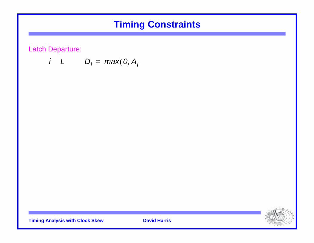
Latch Departure:

i L∈∀ Di max 0 Ai,( )=


Timing Constraints

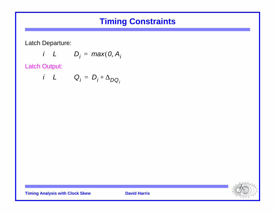
Latch Departure:

Latch Output:


i L∈∀ Qi Di ∆DQ i+=


Timing Constraints

Latch Departure:

Latch Output:

Latch Arrival:



i j L∈,∀ Ai max Qj ∆ji Spjpi+ +( )=


Timing Constraints

Latch Departure:

Latch Output:

Latch Arrival:

Propagation Constraints:




i j L∈,∀ Di max 0 max Dj ∆DQ j∆ji Spjpi

+ + +( ),( )=


Timing Constraints

Latch Departure:

Latch Output:

Latch Arrival:

Propagation Constraints:

Setup Constraints:





+ + +( ),( )=

i L∈∀ Di ∆DC iTpi

≤+


Timing Analysis with Clock Skew

Clock skew is the difference between nominal and actual interarrival times of a pair of clocks.

Enlarge set of physical clocks C to model skew between nominally identical clocks.Example:

∆4

∆5

∆6

∆7

φ1a

φ2a

φ1b

φ2b

φ2a

ALU (clock domain a) Data Cache (clock domain b)

D4

D5

D3

D6

D7

L3

L4

L5

L6

L7

tskewlocal

tskewglobal between domains

within domains

C = {φ1a, φ2a, φ1b, φ2b}


Single Skew Formulation

Easy and conservative to budget global skew everywhere

Effectively increases setup time at each latch

Too conservative for high-speed designs with big global skews

Setup Constraints:

i L∈∀ Di ∆DC itskewglobal+ Tpi

≤+


Exact Skew Budgets

How much skew must be budgeted? • L3 to L4: local skew

∆4

∆5

∆6

∆7

φ1a

φ2a

φ1b

φ2b

φ2a


D4

D5

D3

D6

D7

L3

L4

L5

L6

L7


Exact Skew Budgets

How much skew must be budgeted?• L3 to L4: local skew• L7 to L4: global skew

∆4

∆5

∆6

∆7

φ1a

φ2a

φ1b

φ2b

φ2a


D4

D5

D3

D6

D7

L3

L4

L5

L6

L7


Exact Skew Budgets

How much skew must be budgeted?• L3 to L4: local skew• L7 to L4: global skew• L5 to L4 through transparent L6, L7: local skew

Must track launching clock to determine skew budget

∆4

∆5

∆6

∆7

φ1a

φ2a

φ1b

φ2b

φ2a


D4

D5

D3

D6

D7

L3

L4

L5

L6

L7


Exact Skew Formulation

Define arrival and departure times with respect to launching clocks:: arrival time at latch i for path launched by clock c: departure time from latch i for path launched by clock c

: skew between clocks φi, φj

Aic

Dic

tskewφi φj,


Negative Departure Times

Must now allow negative departure times with respect to other clocks:• Path from L5 to L7 is earlier than L6 to L7, but sees more skew, miss setup• Reaches L6 at -50 ps, but L6 may be transparent by then because of skew

Departure times w.r.t. latch’s own clock still must be nonnegative

∆4

∆5

∆6

∆7

φ1a

φ2a

φ1b

φ2b

φ2a


L3

L4

L5

L6

L7

450 ps

950 pstskew1b 2b, 25 ps=

tskew2a 2b, 150 ps=

∆DC 0=

∆DQ 0=

Tc = 1000 ps

D71b 450=

D72a 400=

D61b 0=

D62a 50–=


Exact Constraints with Skew:

Propagation Constraints (single skew):

Setup Constraints (single skew):

Propagation Constraints (exact skew):

Setup Constraints (exact skew):


+ + +( ),( )=

i L∈∀ Di ∆DC itskewglobal+ Tpi

≤+

i j L c C∈,∈,∀ if c = pi

then Dic max 0 max Dj

c ∆DQ j∆ji Spjpi

+ + +( ),( )=

else D ic max Dj

c ∆DQ j∆ji Spjpi

+ + +( )=

i L c C∈,∈∀ Dic ∆DC i

tskewc pi,

Tpi≤+ +


Other Timing Constraints

Flip-flops:• No transparency, easier than latches• Still budget skew between launching and receiving clocks

Min-delay:• Only requires checks between consecutive pairs of clocked elements• Standard verification algorithms work if proper skew is used


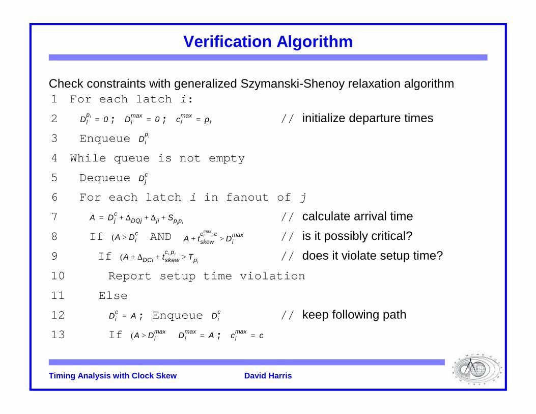
Verification Algorithm

Check constraints with generalized Szymanski-Shenoy relaxation algorithm1 For each latch i:2 ; ; // initialize departure times

3 Enqueue 4 While queue is not empty5 Dequeue 6 For each latch i in fanout of j7 // calculate arrival time

8 If AND // is it possibly critical?

9 If // does it violate setup time?

10 Report setup time violation11 Else12 ; Enqueue // keep following path

13 If ;

Dipi 0= Di

max 0= cimax pi=

Dipi

Djc

A D jc ∆DQj ∆ji Spjpi

+ + +=

A Dic>( ) A tskew

cimax c,

Dimax>+

A ∆DCi tskewc p i,

Tpi>+ +( )

Dic A= Di

c

A Dimax>( ) Di

max A= cimax c=


Results

Analyzed MAGIC: Memory & General Interconnect Controller of FLASH supercomputer

Assume

Model A: • As designed, from MAGIC .sdf database

Model B: • Flops converted to latch pairs, logic balanced between pairs

tskewlocal 250ps= tskew

global 500ps=


Results

Analyzed MAGIC: Memory & General Interconnect Controller of FLASH supercomputer

Assume

Model A: • As designed, from MAGIC .sdf database

Model B: • Flops converted to latch pairs, logic balanced between pairs

CPU time < 1 second in all cases

Model A Model B

# Flip-Flops 10559 0

# Latches 1819 22937

Single Skew Tc 9.43 ns 8.05 ns

# Latch Departures Checked 3866 24995

Exact Skew Tc 9.38 7.96

# Latch Departures Checked 4009 25328

tskewlocal 250ps= tskew

global 500ps=


Conclusions

Global skews will be too large for GHz + systems• Use skew-tolerant circuit techniques such as latches• Take advantage of smaller local skews where possible

Requires support of timing analyzer• Budget appropriate skew at each receiver• Track departure times with respect to launching clocks• Allow negative departure times with respect to other clocks

Leads to explosion in number of timing constraints. However...• Most are not tight because most critical paths do not borrow time across

many latches• Relaxation algorithm automatically prunes loose constraints• Very small increase in runtime

Expect synchronous systems well beyond 1 GHz

timing analysis with clock skew - harvey mudd...

Documents