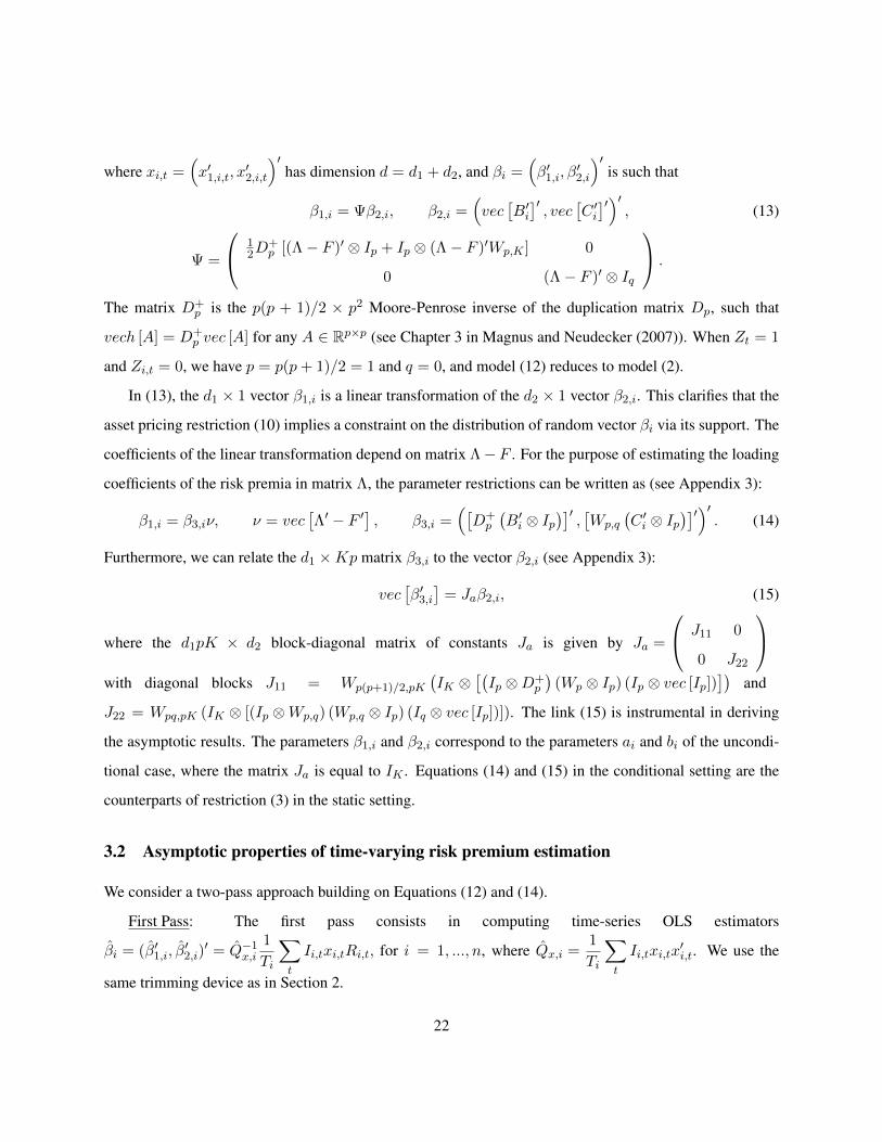
TIME-VARYING RISK PREMIUM IN LARGE

CROSS-SECTIONAL EQUITY DATASETS

Patrick Gagliardinia, Elisa Ossolab and Olivier Scailletc*

First draft: December 2010

This version: November 2011

Abstract

We develop an econometric methodology to infer the path of risk premia from large unbalanced

panel of individual stock returns. We estimate the time-varying risk premia implied by conditional linear

asset pricing models where the conditioning includes instruments common to all assets and asset specific

instruments. The estimator uses simple weighted two-pass cross-sectional regressions, and we show its

consistency and asymptotic normality under increasing cross-sectional and time series dimensions. We

address consistent estimation of the asymptotic variance, and testing for asset pricing restrictions induced

by the no-arbitrage assumption in large economies. The empirical illustration on returns for about ten

thousands US stocks from July 1964 to December 2009 shows that conditional risk premia are large and

volatile in crisis periods. They exhibit large positive and negative strays from standard unconditional

estimates and follow the macroeconomic cycles. The asset pricing restrictions are rejected for the usual

unconditional four-factor model capturing market, size, value and momentum effects.

JEL Classification: C12, C13, C23, C51, C52 , G12.

Keywords: large panel, factor model, risk premium, asset pricing.

aUniversity of Lugano and Swiss Finance Institute, bUniversity of Lugano, cUniversity of Genèva and Swiss Finance Institute.

*Acknowledgements: We gratefully acknowledge the financial support of the Swiss National Science Foundation (Prodoc project

PDFM11-114533 and NCCR FINRISK). We thank Y. Amihud, A. Buraschi, V. Chernozhukov, R. Engle, J. Fan, E. Ghysels, C.

Gouriéroux, S. Heston, participants at the Cass conference 2010, CIRPEE conference 2011, ECARES conference 2011, CORE

conference 2011, Montreal panel data conference 2011, ESEM 2011, and participants at seminars at Columbia, NYU, Georgetown,

Maryland, McGill, GWU, ULB, UCL, Humboldt, Orléans, Imperial College, CREST, Athens, CORE, Bernheim center, for helpful

comments.

1

1 Introduction

Risk premia measure financial compensation asked by investors for bearing risk. Risk is influenced by

financial and macroeconomic variables. Conditional linear factor models aim at capturing their time-varying

influence in a simple setting (see e.g. Shanken (1990), Cochrane (1996), Ferson and Schadt (1996), Ferson

and Harvey (1991, 1999), Lettau and Ludvigson (2001), Petkova and Zhang (2005)). Time variation in risk

is known to bias unconditional estimates of alphas and betas, and therefore asset pricing test conclusions

(Jagannathan and Wang (1996), Lewellen and Nagel (2006), Boguth, Carlson, Fisher and Simutin (2010)).

Ghysels (1998) discusses the pros and cons of modeling time-varying betas.

The workhorse to estimate equity risk premia in a linear multi-factor setting is the two-pass cross-

sectional regression method developed by Black, Jensen and Scholes (1972) and Fama and MacBeth (1973).

Its large and finite sample properties for unconditional linear factor models have been addressed in a series

of papers, see e.g. Shanken (1985, 1992), Jagannathan and Wang (1998), Shanken and Zhou (2007), Kan,

Robotti and Shanken (2009), and the review paper of Jagannathan, Skoulakis and Wang (2009). Statistical

inference for equity risk premia in conditional linear factor model has not yet been formally addressed in

the literature despite its empirical relevance.

In this paper we study how we can infer the time-varying behaviour of equity risk premia from large

stock return databases by using conditional linear factor models. Our approach is inspired by the recent trend

in macro-econometrics and forecasting methods trying to extract cross-sectional and time-series information

simultaneously from large panels (see e.g. Stock and Watson (2002a,b), Bai (2003, 2009), Bai and Ng

(2002, 2006), Forni, Hallin, Lippi and Reichlin (2000, 2004, 2005), Pesaran (2006)). Ludvigson and Ng

(2007, 2009) show that it is a promising route to follow to study bond risk premia. Connor, Hagmann,

and Linton (2011) show that large cross-section helps to exploit data more efficiently in a semiparametric

characteristic-based factor model of stock returns. It is also inspired by the framework underlying the

Arbitrage Pricing Theory (APT). Approximate factor structures with nondiagonal error covariance matrices

(Chamberlain and Rothschild (1983, CR)) address the potential empirical mismatch of exact factor structures

with diagonal error covariance matrices underlying the original APT of Ross (1976). Under weak cross-

sectional dependence among error terms, they generate no-arbitrage restrictions in large economies where

the number of assets grows to infinity. Our paper develops an econometric methodology tailored to the APT

2

framework. We let the number of assets grow to infinity mimicking the large economies of financial theory.

Our approach is further motivated by the potential loss of information and bias induced by grouping

stocks to build portfolios in asset pricing tests (Litzenberger and Ramaswamy (1979), Lo and MacKinlay

(1990), Berk (2000), Conrad, Cooper and Kaul (2003), Phalippou (2007)). Avramov and Chordia (2006)

have already shown that empirical findings given by conditional factor models about anomalies differ a

lot when considering single securities instead of portfolios. Ang, Liu and Schwarz (2008) argue that a lot

of efficiency may be lost when only considering portfolios as base assets, instead of individual stocks, to

estimate equity risk premia in unconditional models. In our approach the large cross-section of stock returns

also helps to get accurate estimation of the equity risk premia even if we get noisy time-series estimates

of the factor loadings (the betas). Besides, when running asset-pricing tests, Lewellen, Nagel and Shanken

(2010) advocate working with a large number of assets instead of working with a small number of portfolios

exhibiting a tight factor structure. The former gives us a higher hurdle to meet in judging model explanation

based on cross-sectional R2.

Our theoretical contributions are threefold. First we derive no-arbitrage restrictions in a multi-period

economy (Hansen and Richard (1987)) with a continuum of assets and an approximate factor structure

(Chamberlain and Rothschild (1983)). We explicitly show the relationship between the ruling out of asymp-

totic arbitrage opportunities and a testable restriction for large economies in a conditional setting. We also

formalize the sampling scheme when observed assets are random draws from an underlying population (An-

drews (2005)). Second we derive a new weighted two-pass cross-sectional estimator of the path over time

of the risk premia from large unbalanced panels of excess returns. We study its large sample properties

in conditional linear factor models where the conditioning includes instruments common to all assets and

asset specific instruments. The factor modeling permits conditional heteroskedasticity and cross-sectional

dependence in the error terms (see Petersen (2008) for stressing the importance of residual dependence when

computing standard errors in finance panel data). We derive consistency and asymptotic normality of our

estimates by letting the time dimension T and the cross-section dimension n grow to infinity simultane-

ously, and not sequentially. We relate the results to bias-corrected estimation (Hahn and Kuersteiner (2002),

Hahn and Newey (2004)) accounting for the well-known incidental parameter problem of the panel literature

(Neyman and Scott (1948)). We derive all properties for unbalanced panels to avoid the survivorship bias

3

inherent to studies restricted to balanced subsets of available stock return databases (Brown, Goetzmann,

Ross (1995)). The two-pass regression approach is simple and particularly easy to implement in an unbal-

anced setting. This explains our choice over more efficient, but numerically intractable, one-pass ML/GMM

estimators or generalized least-squares estimators. When n is of the order of a couple of thousands assets,

numerical optimization on a large parameter set or numerical inversion of a large weighting matrix is too

challenging and unstable to benefit in practice from the theoretical efficiency gains, unless imposing strong

ad hoc structural restrictions. Third we provide a goodness-of-fit test for the conditional factor model un-

derlying the estimation. The test exploits the asymptotic distribution of a weighted sum of squared residuals

of the second-pass cross-sectional regression (see Lewellen, Nagel and Shanken (2010), Kan, Robotti and

Shanken (2009) for a related approach in unconditional models and asymptotics with fixed n). The con-

struction of the test statistic relies on consistent estimation of large-dimensional sparse covariance matrices

by thresholding (Bickel and Levina (2008), El Karoui (2008), Fan, Liao, and Mincheva (2011)). As a by-

product, our approach permits inference for the cost of equity on individual stocks, in a time-varying setting

(Fama and French (1997)). As known from standard textbooks in corporate finance, the cost of equity is

such that cost of equity = risk free rate + factor loadings × factor risk premia. It is part of the cost of capital

and is a central piece for evaluating investment projects by company managers. For pedagogical purposes

the three theoretical contributions are first presented in an unconditional setting before being extended to a

conditional setting.

For our empirical contributions, we consider the Center for Research in Security Prices (CRSP) database

and take the Compustat database to match firm characteristics. The merged dataset comprises about ten

thousands stocks with monthly returns from July 1964 to December 2009. We look at factor models popular

in the empirical finance literature to explain monthly equity returns. They differ by the choice of the factors.

The first model is the CAPM (Sharpe (1964), Lintner (1965)) using market return as the single factor. Then,

we consider the three-factor model of Fama and French (1993) based on two additional factors capturing the

book-to-market and size effects, and a four-factor extension including a momentum factor (Jegadeesh and

Titman (1993), Carhart (1997)). We study both unconditional and conditional factor models (Ferson and

Schadt (1996), and Ferson and Harvey (1999)). For the conditional versions we use both macrovariables

and firm characteristics as instruments. The estimated path shows that the risk premia are large and volatile

4

in crisis periods, e.g., the oil crisis in 1973-1974, the market crash in October 1987, and the crisis of the

recent years. Furthermore, the conditional estimates exhibit large positive and negative strays from standard

unconditional estimates and follow the macroeconomic cycles. The asset pricing restrictions are rejected for

the usual unconditional four-factor model capturing market, size, value and momentum effects.

The outline of the paper is as follows. In Section 2 we present our approach in an unconditional lin-

ear factor setting. In Section 3 we extend all results to cover a conditional linear factor model where the

instruments inducing time varying coefficients can be common to all stocks or stock specific. Section 4

contains the empirical results. Section 5 contains the simulation results. Finally, Section 6 concludes. In

the Appendix, we gather the technical assumptions and some proofs. We place all omitted proofs in the

online supplementary materials. We use high-level assumptions to get our results and show in Appendix 4

that they are all met under a block cross-sectional dependence structure on the error terms in a serially i.i.d.

framework.

2 Unconditional factor model

In this section we consider an unconditional linear factor model in order to illustrate the main contributions

of the article in a simple setting. This covers the CAPM where the single factor is the excess market return.

2.1 Excess return generation and asset pricing restrictions

We start by describing how excess returns are generated before examining the implications of absence of ar-

bitrage opportunities in terms of restrictions on the return generating process. We combine the constructions

of Hansen and Richard (1987) and Andrews (2005) to define a multi-period economy with a continuum of

assets having strictly stationary and ergodic return processes. We use such a formal construction to guar-

antee that (i) the economy is invariant to time shifts, so that we can establish all properties by working at

t = 1, (ii) time series averages converge almost surely to population expectations, (iii) under a sampling

mechanism (see the next section) cross-sectional limits exist and are invariant to reordering of the assets,

and (iv) the derived no-arbitrage restriction is empirically testable.

Let (Ω,F , P ) be a probability space. The random vector f admitting values in RK , and the collection

5

of random variables ε(γ), γ ∈ [0, 1], are defined on this probability space. Moreover, let β = (a, b′)′ be

a vector function defined on [0, 1] with values in R × RK . The dynamics is described by the measurable

time-shift transformation S mapping Ω into itself. If ω ∈ Ω is the state of the world at time 0, then St(ω) is

the state at time t, where St denotes the transformation S applied t times successively. Transformation S is

assumed to be measure-preserving and ergodic (i.e., any set in F invariant under S has measure either 1, or

0).

Assumption APR.1 The excess returns Rt(γ) of asset γ ∈ [0, 1] at date t = 1, 2, ... satisfy the uncondi-

tional linear factor model:

Rt(γ) = a(γ) + b(γ)′ft + εt(γ), (1)

where the random variables εt(γ) and ft are defined by εt (γ, ω) = ε[γ, St(ω)] and ft(ω) = f [St(ω)].

Assumption APR.1 defines the excess return processes for an economy with a continuum of assets. The

index set is the interval [0, 1] without loss of generality. Vector ft gathers the values of the K observable

factors at date t, while the intercept a(γ) and factor sensitivities b(γ) of asset γ ∈ [0, 1] are time invariant.

Since transformation S is measure-preserving and ergodic, all processes are strictly stationary and ergodic

(Doob (1953)). Let further define xt = (1, f′t )

′which yields the compact formulation:

Rt(γ) = β(γ)′xt + εt(γ). (2)

In order to define the information sets, let F0 ⊂ F be a sub sigma-field. Random vector f is assumed

measurable w.r.t. F0. Define Ft = S−t (A) , A ∈ F0, t = 1, 2, ..., and assume that F1 contains F0. Then,

the filtration Ft, t = 1, 2, ..., characterizes the information available to investors.

Let us now introduce supplementary assumptions on factors, factor loadings and error terms.

Assumption APR.2 The matrixˆb(γ)b(γ)′dγ is positive definite.

Assumption APR.2 implies non-degeneracy in the factor loadings across assets.

Assumption APR.3 For any γ ∈ [0, 1]: E[εt(γ)|Ft−1] = 0 and Cov[εt(γ), ft|Ft−1] = 0.

6

Hence, the error terms have mean zero and are uncorrelated with the factors conditionally on information

Ft−1. In Assumption APR.4 (i) below, we impose an approximate factor structure for the conditional

distribution of the error terms given Ft−1 in almost any countable collection of assets. More precisely, for

any sequence (γi) in [0, 1], let Σε,t,n denote the n × n conditional variance-covariance matrix of the error

vector [εt(γ1), ..., εt(γn)]′ given Ft−1, for n ∈ N. Let µΓ be the probability measure on the set Γ = [0, 1]N

of sequences (γi) in [0, 1] induced by i.i.d. random sampling from a continuous distribution G with support

[0, 1].

Assumption APR.4 For any sequence (γi) in set J : (i) eigmax (Σε,t,n) = o(n), as n → ∞, P -a.s.,

(ii) infn≥1

eigmin (Σε,t,n) > 0, P -a.s., where J ⊂ Γ is such that µΓ(J ) = 1, and eigmin (Σε,t,n) and

eigmax (Σε,t,n) denote the smallest and the largest eigenvalues of matrix Σε,t,n, (iii) eigmin (V [ft|Ft−1]) >

0, P -a.s.

Assumption APR.4 (i) is weaker than boundedness of the largest eigenvalue, i.e., supn≥1

eigmax (Σε,t,n) <∞,

P -a.s., as in CR. This is useful for the checks of Appendix 4 under a block cross-sectional dependence

structure. Assumptions APR.4 (ii)-(iii) are mild regularity conditions used in the proof of Proposition 1.

Absence of asymptotic arbitrage opportunities generates asset pricing restrictions in large economies

(Ross (1976), CR). We define asymptotic arbitrage opportunities in terms of sequences of portfolios pn,

n ∈ N. Portfolio pn is defined by the share α0,n invested in the riskfree asset and the shares αi,n invested in

the selected risky assets γi, for i = 1, ...., n. The shares are measurable w.r.t. F0. Then C(pn) =

n∑i=0

αi,n is

the portfolio cost at t = 0, and pn = C(pn)R0 +

n∑i=1

αi,nR1(γi) is the portfolio payoff at t = 1, where R0

denotes the riskfree gross return measurable w.r.t. F0. We can work with t = 1 because of stationarity.

Assumption APR.5 There are no asymptotic arbitrage opportunities in the economy, that is, there exists

no portfolio sequence (pn) such that limn→∞

P [pn ≥ 0] = 1 and limn→∞

P [C(pn) ≤ 0, pn > 0] > 0.

Assumption APR.5 excludes portfolios that approximate arbitrage opportunities when the number of

included assets increases. Arbitrage opportunities are investments with non-positive cost and non-negative

payoff in each state of the world, and positive payoff in some states of the world (Hansen and Richard

(1987), Definition 2.4). Then, the asset pricing restriction is given in the next Proposition 1.

7

Proposition 1 Under Assumptions APR.1-APR.5, there exists a unique vector ν ∈ RK such that:

a(γ) = b(γ)′ν, (3)

for almost all γ ∈ [0, 1].

The asset pricing restriction in Proposition 1 can be rewritten as

E [Rt(γ)] = b(γ)′λ, (4)

for almost all γ ∈ [0, 1], where λ = ν + E [ft] is the vector of the risk premia. In the CAPM, we have

K = 1 and ν = 0. When a factor fk,t is a portfolio excess return, we also have νk = 0, k = 1, ...,K.

Proposition 1 differs from CR Theorem 3 in terms of the returns generating framework, the definition

of asymptotic arbitrage opportunities, and the derived asset pricing restriction. Specifically, we consider a

multi-period economy with conditional information as opposed to a single period unconditional economy as

in CR. Such a setting can be easily extended to time varying risk premia in Section 3. We prefer the definition

underlying Assumption APR.5 since it corresponds to the definition of arbitrage that is standard in dynamic

asset pricing theory (e.g., Duffie (2001)). As pointed out by Hansen and Richard (1987), Ross (1978) has

already chosen that type of definition. It also eases the proof. However, in Appendix 2, we derive the link

between the no-arbitrage conditions in Assumptions A.1 i) and ii) of CR, written P -a.s. w.r.t. the conditional

information F0 and for almost every countable collection of assets, and the asset pricing restriction (3) valid

for the continuum of assets. Hence, we are able to characterize the functions β = (a, b′)′ defined on [0, 1]

that are compatible with absence of asymptotic arbitrage opportunities under both definitions of arbitrage in

the continuum economy. CR derive the pricing restriction∞∑i=1

(a(γi)− b(γi)

′ν)2

<∞, for some ν ∈ RK

and for a given sequence (γi), while we derive the restriction (3), for almost all γ ∈ [0, 1]. In Appendix 2,

we show that the set of sequences (γi) such that infν∈RK

∞∑i=1

(a(γi)− b(γi)

′ν)2

<∞ has measure 1 under

µΓ, when the asset pricing restriction (3) holds, and measure 0, otherwise. This result is a consequence

of the Kolmogorov zero-one law (see e.g. Billingsley (1995)). In other words, validity of the summability

condition in CR for a countable collection of assets without validity of the asset pricing restriction (3) is an

impossible event. From the proofs in Appendix 2, we can also see that, when the asset pricing restriction

8

(3) does not hold, asymptotic arbitrage in the sense of Assumption APR.5, or of Assumptions A.1 i) and ii)

of CR, exists for µΓ-almost any countable collection of assets. The restriction in Proposition 1 is testable

with large equity datasets and large sample sizes (Section 2.5), and therefore is not affected by the Shanken

(1982) critique. The next section describes how we get the data from sampling the continuum of assets.

2.2 The sampling scheme

We estimate the risk premia from a sample of observations on returns and factors for n assets and T dates. In

available databases, asset returns are not observed for all firms at all dates. We account for the unbalanced

nature of the panel through a collection of indicator variables I(γ), γ ∈ [0, 1], and define It(γ, ω) =

I[γ, St(ω)]. Then It(γ) = 1 if the return of asset γ is observable by the econometrician at date t, and

0 otherwise (Connor and Korajczyk (1987)). To ease exposition and to keep the factor structure linear,

we assume a missing-at-random design (Rubin (1976), Heckman (1979)), that is, independence between

unobservability and returns generation.

Assumption SC.1 The random variables It(γ), γ ∈ [0, 1], are independent of εt(γ), γ ∈ [0, 1], and ft.

Another design would require an explicit modeling of the link between the unobservability mechanism and

the continuum of assets; this would yield a nonlinear factor structure.

Assets are randomly drawn from the population according to a probability distribution G on [0, 1]. We

use a single distribution G in order to avoid the notational burden when working with different distributions

on different subintervals of [0, 1].

Assumption SC.2 The random variables γi, i = 1, ..., n, are i.i.d. indices, independent of εt(γ), It(γ),

γ ∈ [0, 1] and ft, each with continuous distribution G with support [0, 1].

For any n, T ∈ N, the excess returns are Ri,t = Rt(γi) and the observability indicators are Ii,t = It(γi),

for i = 1, ..., n, and t = 1, ..., T . The excess return Ri,t is observed if and only if Ii,t = 1. Similarly, let

βi = β(γi) = (ai, b′i)′ be the characteristics, εi,t = εt(γi) the error terms and σij,t = E[εi,tεj,t|xt, γi, γj ]

the conditional variances and covariances of the assets in the sample, where xt = xt, xt−1, .... By random

sampling, we get a random coefficient panel model (e.g. Wooldridge (2002)). The characteristic βi of asset

9

i is random, and potentially correlated with the error terms εi,t and the observability indicators Ii,t, as well

as the conditional variances σii,t, through the index γi. If the ais and bis were treated as deterministic, and

not as realizations of random variables, invoking cross-sectional LLNs and CLTs as in some assumptions

and parts of the proofs would have no sense. Moreover, cross-sectional limits would be dependent on the

selected ordering of the assets. Instead, our assumptions and results do not rely on a specific ordering of

assets. Random elements (β′i, σii,t, εi,t, Ii,t)′, i = 1, ..., n, are exchangeable (Andrews (2005)). Hence,

assets randomly drawn from the population have ex-ante the same features. However, given a specific

realization of the indices in the sample, assets have ex-post heterogeneous features.

2.3 Asymptotic properties of risk premium estimation

We consider a two-pass approach (Fama and MacBeth (1973), Black, Jensen and Scholes (1972)) building

on Equations (1) and (3).

First Pass: The first pass consists in computing time-series OLS estimators

βi = (ai, b′i)′ = Q−1

x,i

1

Ti

∑t

Ii,txtRi,t, for i = 1, ..., n, where Qx,i =1

Ti

∑t

Ii,txtx′t and Ti =

∑t

Ii,t. In

available panels the random sample size Ti for asset i can be small, and the inversion of matrix Qx,i can be

numerically unstable. This can yield unreliable estimates of βi. To address this, we introduce a trimming de-

vice: 1χi = 1CN

(Qx,i

)≤ χ1,T , τi,T ≤ χ2,T

, where CN

(Qx,i

)=

√eigmax

(Qx,i

)/eigmin

(Qx,i

)denotes the condition number of matrix Qx,i, τi,T = T/Ti, and the two sequences χ1,T > 0 and χ2,T > 0

diverge asymptotically. The first trimming condition CN(Qx,i

)≤ χ1,T keeps in the cross-section only

assets for which the time series regression is not too badly conditioned. A too large value of CN(Qx,i

)=

1/CN(Q−1x,i

)indicates multicollinearity problems and ill-conditioning (Belsley, Kuh, and Welsch (2004),

Greene (2008)). The second trimming condition τi,T ≤ χ2,T keeps in the cross-section only assets for

which the time series is not too short.

Second Pass: The second pass consists in computing a cross-sectional estimator of ν by regressing the

ai’s on the bi’s keeping the non-trimmed assets only. We use a WLS approach. The weights are esti-

mates of wi = v−1i , where the vi are the asymptotic variances of the standardized errors

√T(ai − b′iν

)in the cross-sectional regression for large T . We have vi = τic

′νQ−1x SiiQ

−1x cν , where Qx = E

[xtx′t

],

Sii = plimT→∞

1

T

∑t

σii,txtx′t = E

[ε2i,txtx

′t|γi], τi = plim

T→∞τi,T = E[Ii,t|γi]−1, and cν = (1,−ν ′)′. We use

10

the estimates vi = τi,T c′ν1Q

−1x,i SiiQ

−1x,icν1 , where Sii =

1

Ti

∑t

Ii,tε2i,txtx

′t, εi,t = Ri,t − β′ixt and cν1 =

(1,−ν ′1)′. To estimate cν , we use the OLS estimator ν1 =

(∑i

1χi bib′i

)−1∑i

1χi biai, i.e., a first-step

estimator with unit weights. The WLS estimator is:

ν = Q−1b

1

n

∑i

wibiai, (5)

where Qb =1

n

∑i

wibib′i and wi = 1χi v

−1i . Weighting accounts for the statistical precision of the first-

pass estimates. Under conditional homoskedasticity σii,t = σii and a balanced panel τi,T = 1, we have

vi = c′νQ−1x cνσii. There, vi is directly proportional to σii, and we can simply pick the weights as wi = σ−1

ii ,

where σii =1

T

∑t

ε2i,t (Shanken (1992)). The final estimator of the risk premia is

λ = ν +1

T

∑t

ft. (6)

Starting from the asset pricing restriction (4), another estimator of λ is λ = Q−1b

1

n

∑i

wibiRi, where

Ri =1

Ti

∑t

Ii,tRi,t. This estimator is numerically equivalent to λ in the balanced case, where Ii,t = 1 for

all i and t. In the general unbalanced case, it is equal to λ = ν + Q−1b

1

n

∑i

wibib′ifi,where fi =

1

Ti

∑t

Ii,tft.

Estimator λ is often studied by the literature (see, e.g., Shanken (1992), Kandel and Stambaugh (1995), Ja-

gannathan and Wang (1998)), and is also consistent. EstimatingE [ft] with a simple average of the observed

factor instead of a weighted average based on estimated betas simplifies the form of the asymptotic distri-

bution in the unbalanced case (see below and Section 2.4). This explains our preference for λ over λ.

We derive the asymptotic properties under assumptions on the conditional distribution of the error terms.

Assumption A.1 There exists a positive constant M such that for all n:

a) E[εi,t|εj,t−1, γj , j = 1, ..., n, xt

]= 0, with εi,t−1 = εi,t−1, εi,t−2, · · · and xt = xt, xt−1, · · · ;

b) σii,t ≤M, i = 1, ..., n; c) E

1

n

∑i,j

|σij,t|

≤M , where σij,t = E[εi,tεj,t|xt, γi, γj

].

Assumption A.1 allows for a martingale difference sequence for the error terms (part a)) including potential

conditional heteroskedasticity (part b)) as well as weak cross-sectional dependence (part c)). In particular,

11

Assumption A.1 c) is the same as Assumption C.3 in Bai and Ng (2002)), except that we have an expectation

w.r.t. the random draws of assets. More general error structures are possible but complicate consistent

estimation of the asymptotic variances of the estimators (see Section 2.4).

Proposition 2 summarizes consistency of estimators ν and λ under the double asymptotics

n, T → ∞. For sequences xn and yn, we denote xn yn when xn/yn is bounded and bounded away

from zero from below as n→∞.

Proposition 2 Under Assumptions APR.1-APR.5, SC.1-SC.2, A.1 and C.1a), C.2-C.5, we get a) ‖ν − ν‖ =

op (1) and b)∥∥∥λ− λ∥∥∥ = op (1), when n, T →∞ such that n T γ for γ > 0.

The conditions in Proposition 2 allow for n large w.r.t. T (short panel asymptotics) when γ > 1. Shanken

(1992) shows consistency of ν and λ for a fixed n and T →∞. This consistency does not imply Proposition

2. Shanken (1992) (see also Litzenberger and Ramaswamy (1979)) further shows that we can estimate ν

consistently in the second pass with a modified cross-sectional estimator for a fixed T and n → ∞. Since

λ = ν+E [ft], consistent estimation of the risk premia themselves is impossible for a fixed T (see Shanken

(1992) for the same point).

Proposition 3 below gives the large-sample distributions under the double asymptotics

n, T → ∞. Let us define τij,T = T/Tij , where Tij =∑t

Iij,t and Iij,t = Ii,tIj,t for i, j = 1, ..., n. Let us

further define τij = plimT→∞

τij,T = E[Iij,t|γi, γj ]−1, Sij = plimT→∞

1

T

∑t

σij,txtx′t = E[εi,tεj,txtx

′t|γi, γj ] and

Qb = plimn→∞

1

n

∑i

wibib′i = E[wibib

′i]. The following assumption describes the CLTs underlying the proof

of the distributional properties. These CLTs hold under weak serial and cross-sectional dependencies such

as temporal mixing and block dependence (see Appendix 4).

Assumption A.2 As n, T → ∞ such that n T γ for γ ∈ Γ1 ⊂ R+, a)1√n

∑i

wiτi (Yi,T ⊗ bi)⇒

N (0, Sb) , where Yi,T =1√T

∑t

Ii,txtεi,t and Sb = limn→∞

E

1

n

∑i,j

wiwjτiτjτij

Sij ⊗ bib′j

= plim

n→∞

1

n

∑i,j

wiwjτiτjτij

Sij ⊗ bib′j ; b)1√T

∑t

(ft − E [ft])⇒N (0,Σf ) ,where Σf = limT→∞

1

T

∑t,s

Cov (ft, fs) .

12

Proposition 3 Under Assumptions APR.1-APR.5, SC.1-SC.2, A.1-A.2, and C.1a), C.2-C.5, we get:

a)√nT

(ν − ν − 1

TBν

)⇒N (0,Σν) ,where Σν = Q−1

b limn→∞

E

1

n

∑i,j

wiwjτiτjτij

(c′νQ−1x SijQ

−1x cν)bib

′j

Q−1b

and the bias term is Bν = Q−1b

(1

n

∑i

wiτi,TE′2Q−1x,i SiiQ

−1x,icν

), withE2 = (0 : IdK)′ and cν = (1,−ν ′)′;

b)√T(λ− λ

)⇒ N (0,Σf ), when n, T →∞ such that n T γ for γ ∈ Γ1 ∩ (0, 3) .

The asymptotic variance matrix in Proposition 3 can be rewritten as:

Σν = plimn→∞

(1

nB′nWnBn

)−1 1

nB′nWnVnWnBn

(1

nB′nWnBn

)−1

where Bn = (b1, ..., bn)′, Wn = diag(w1, ..., wn) and Vn = [vij ]i,j=1,...,n with vij =τiτjτij

c′νQ−1x SijQ

−1x cν ,

which gives vii = vi. In the homoskedastic and balanced case, we have c′νQ−1x cν = 1 + λ′V [ft]

−1λ and

Vn = (1 + λ′V [ft]−1λ)Σε,n, where Σε,n = [σij ]i,j=1,...,n. Then, the asymptotic variance of ν reduces

to plimn→∞

(1 + λ′V [ft]−1λ)

(1

nB′nWnBn

)−1 1

nB′nWnΣε,nWnBn

(1

nB′nWnBn

)−1

. In particular, in the

CAPM we have K = 1 and ν = 0, which implies that

√λ2

V [ft]is equal to the slope of the Capital Market

Line

√E[ft]2

V [ft], i.e., the Sharpe Ratio of the market portfolio.

Proposition 3 shows that the estimator ν has a fast convergence rate√nT and features an asymptotic

bias term. Both ai and bi in the definition of ν contain an estimation error; for bi, this is the well-known

Error-In-Variable (EIV) problem. The EIV problem does not impede consistency since we let T grow to

infinity. However, it induces the bias term Bν/T which centers the asymptotic distribution of ν. We have

Γ1 = R+ in Assumption A.2, when (εi,t) and (xt) are i.i.d. across time and errors (εi,t) feature a cross-

sectional block dependence structure (see Appendix 4). Then, the upper bound on the relative expansion

rates of n and T is n = o(T 3). The control of first-pass estimation errors uniformly across assets requires

that the cross-section dimension n should not be too large w.r.t. the time series dimension T .

If we knew the true factor mean, for example E[ft] = 0, and did not need to estimate it, the estimator

ν + E[ft] of the risk premia would have the same fast rate√nT as the estimator of ν, and would inherit

its asymptotic distribution. Since we do not know the true factor mean, the asymptotic distribution of λ is

driven only by the variability of the factor since the convergence rate√T of the sample average

1

T

∑t

ft

13

dominates the convergence rate√nT of ν. This result is an oracle property for λ, namely that its asymptotic

distribution is the same irrespective of the knowledge of ν. This property is in sharp difference with the

single asymptotics with a fixed n and T → ∞. In the balanced case and with homoskedastic errors, Theo-

rem 1 of Shanken (1992) shows that the rate of convergence of λ is√T and that its asymptotic variance is

Σλ,n = Σf + (1 + λ′V [ft]−1λ)

(1

nB′nWnBn

)−1 1

n2B′nWnΣε,nWnBn

(1

nB′nWnBn

)−1

, for fixed n and

T → ∞. The two components in Σλ,n come from estimation of E[ft] and ν, respectively. In the het-

eroskedastic setting with fixed n, a slight extension of Theorem 1 in Jagannathan and Wang (1998), or Theo-

rem 3.2 in Jagannathan, Skoulakis, and Wang (2009), to the unbalanced case yields

Σλ,n = Σf +

(1

nB′nWnBn

)−1 1

n2B′nWnVnWnBn

(1

nB′nWnBn

)−1

. Letting n → ∞ gives Σf under

weak cross-sectional dependence. Thus, exploiting the full cross-section of assets improves efficiency

asymptotically, and the positive definite matrix Σλ,n − Σf corresponds to the efficiency gain. Using a

large number of assets instead of a small number of portfolios does help to eliminate the EIV contribution.

Proposition 3 suggests exploiting the analytical bias correction Bν/T and using νB = ν − 1

TBν instead

of ν. Furthermore, λB = νB +1

T

∑t

ft delivers a bias-free estimator of λ at order 1/T , which shares the

same root-T asymptotic distribution as λ.

Finally, we can relate the results of Proposition 3 to bias-corrected estimation accounting for the well-

known incidental parameter problem of the panel literature (Neyman and Scott (1948), see Lancaster (2000)

for a review). Model (1) under restriction (3) can be written as Ri,t = b′i(ft + ν) + εi,t. In the likelihood

setting of Hahn and Newey (2004) (see also Hahn and Kuersteiner (2002)), the bi correspond to the indi-

vidual effects and ν to the common parameter of interest. Available results tell us: (i) the estimator of ν is

inconsistent if n goes to infinity while T is held fixed; (ii) the estimator of ν is asymptotically biased even

if T grows at the same rate as n; (iii) an analytical bias correction may yield an estimator of ν that is root-

(nT ) asymptotically normal and centered at the truth if T grows faster than n1/3. The two-pass estimators

ν and νB exhibits the properties (i)-(iii) as expected by analogy with unbiased estimation in large panels.

This clear link with the incidental parameter literature highlights another advantage of working with ν in

the second pass regression.

14

2.4 Confidence intervals

We can use Proposition 3 to build confidence intervals by means of consistent estimation of the asymptotic

variances. We can check with these intervals whether the risk of a given factor fk,t is not remunerated, i.e.,

λk = 0, or the restriction νk = 0 holds when the factor is traded. We estimate Σf by a standard HAC

estimator Σf such as in Newey and West (1994) or Andrews and Monahan (1992). Hence, the construction

of confidence intervals with valid asymptotic coverage for components of λ is straightforward. On the

contrary, getting a HAC estimator for Σf appearing in the asymptotic distribution of λ is not obvious in the

unbalanced case.

The construction of confidence intervals for the components of ν is more difficult. Indeed, Σν involves

a limiting double sum over Sij scaled by n and not n2. A naive approach consists in replacing Sij by

any consistent estimator such as Sij =1

Tij

∑t

Iij,tεi,tεj,txtx′t, but this does not work here. To handle

this, we rely on recent proposals in the statistical literature on consistent estimation of large-dimensional

sparse covariance matrices by thresholding (Bickel and Levina (2008), El Karoui (2008)). Fan, Liao, and

Mincheva (2011) have recently focused on the estimation ofE[ε′tεt] in large balanced panel with nonrandom

coefficients.

The idea is to assume sparse contributions of the Sij’s to the double sum. Then we only have to account

for sufficiently large contributions in the estimation, i.e., contributions larger than a threshold vanishing

asymptotically. Thresholding permits an estimation invariant to asset permutations; this choice of estimator

is motivated by the absence of any natural cross-sectional ordering among the matrices Sij . In the following

assumption we use the notion of sparsity suggested by Bickel and Levina (2008) adapted to our framework

with random coefficients.

Assumption A.3 There exist constants q, δ ∈ [0, 1) such that maxi

∑j

‖Sij‖q = Op

(nδ)

.

Assumption A.3 tells us that most cross-asset contributions ‖Sij‖ can be neglected. As sparsity increases,

we can choose coefficients q and δ closer to zero. Assumption A.3 does not impose sparsity of the covariance

matrix of the returns themselves. Assumption A.1 c) is also a sparsity condition, which ensures that the limit

matrix Σν is well-defined when combined with Assumption C.3. Both sparsity assumptions, as well as the

approximate factor structure Assumption APR.4 (i), are satisfied under weak cross-sectional dependence

15

between the error terms, for instance, under a block dependence structure (see Appendix 4).

As in Bickel and Levina (2008), let us introduce the thresholded estimator Sij = Sij1∥∥∥Sij∥∥∥ ≥ κ of

Sij , which we refer to as Sij thresholded at κ = κn,T . We can derive an asymptotically valid confidence

interval for the components of ν from the next proposition giving a feasible asymptotic normality result.

Proposition 4 Under Assumptions APR.1-APR.5, SC.1-SC.2, A.1-A.3, C.1-C.5, we have

Σ−1/2ν

√nT

(ν − 1

TBν − ν

)⇒ N (0, IdK) where Σν = Q−1

b

1

n

∑i,j

wiwjτi,T τj,Tτij,T

(c′νQ−1x SijQ

−1x cν)bib

′j

Q−1b ,

when n, T → ∞ such that n T γ for γ ∈ Γ1 ∩(

0,min

1 + η, η

1− q2δ

), and κ = M

√log n

T ηfor a

constant M and η ∈ (0, 1] as in Assumption C.1.

Constant η ∈ (0, 1] is defined in Assumption C.1 and is related to the time series dependence of pro-

cesses (εi,t) and (xt). We have η = 1, when (εi,t) and (xt) are serially i.i.d. as in Appendix 4 and Bickel

and Levina (2008). The matrix made of thresholded blocks Sij is not guaranteed to be semi definite positive

(sdp). However we expect that the double summation on i and j makes Σν sdp in empirical applications. In

case it is not, El Karoui (2008) discusses a few solutions based on shrinkage.

2.5 Tests of asset pricing restrictions

The null hypothesis underlying the asset pricing restriction (3) is

H0 : there exists ν ∈ RK such that a(γ) = b(γ)′ν, for almost all γ ∈ [0, 1].

Under H0, we have EG[(ai − b′iν)2

]= 0. Since ν is estimated via the WLS cross-sectional regression

of the estimates ai on the estimates bi, we suggest a test based on the weighted sum of squared residuals

SSR of the cross-sectional regression. The weigthed SSR is Qe =1

n

∑i

wie2i , with ei = c′ν βi, which is an

empirical counterpart of EG[wi (ai − b′iν)2

].

Let us define Sii,T =1

T

∑t

Ii,tσii,txtx′t, and introduce the commutation matrixWm,n of ordermn×mn

such that Wm,nvec [A] = vec [A′] for any matrix A ∈ Rm×n, where the vector operator vec [·] stacks the

elements of an m×n matrix as a mn× 1 vector. If m = n, we write Wn instead Wn,n. For two (K + 1)×

16

(K + 1) matrices A and B, equality W(K+1) (A⊗B) = (B ⊗A)W(K+1) also holds (see Chapter 3 of

Magnus and Neudecker (2007) for other properties).

Assumption A.4 For n, T → ∞ such that n T γ for γ ∈ Γ2 ⊂ Γ1, we have1√n

∑i

wiτ2i (Yi,T ⊗ Yi,T − vec [Sii,T ])⇒ N (0,Ω), where the asymptotic variance matrix is:

Ω = limn→∞

E

1

n

∑i,j

wiwjτ2i τ

2j

τ2ij

[Sij ⊗ Sij + (Sij ⊗ Sij)W(K+1)

]= plim

n→∞

1

n

∑i,j

wiwjτ2i τ

2j

τ2ij

[Sij ⊗ Sij + (Sij ⊗ Sij)W(K+1)

].

Assumption A.4 is a high-level CLT condition. This assumption can be proved under primitive conditions

on the time series and cross-sectional dependence. For instance, we prove in Appendix 4 that Assumption

A.4 holds under a cross-sectional block dependence structure for the errors. Intuitively, the expression of the

variance-covariance matrix Ω is related to the result that, for random (K + 1)× 1 vectors Y1 and Y2 which

are jointly normal with covariance matrix S, we have Cov (Y1 ⊗ Y1, Y2 ⊗ Y2) = S⊗S+ (S ⊗ S)W(K+1).

Let us now introduce the following statistic ξnT = T√n

(Qe −

1

TBξ

), where the recentering term

simplifies to Bξ = 1 thanks to the weighting scheme. Under the null hypothesis H0, we prove that

ξnT =(vec

[Q−1x cνc

′νQ−1x

])′ 1√n

∑i

wiτ2i (YiT ⊗ Yi,T − vec [Sii,T ]) + op (1), which implies

ξnT ⇒ N (0,Σξ), where Σξ = 2 limn→∞

E

1

n

∑i,j

wiwjv2ij

= 2 plimn→∞

1

n

∑i,j

wiwjv2ij as n, T → ∞ (see

Appendix A.2.5). Then a feasible testing procedure exploits the consistent estimator Σξ = 21

n

∑i,j

wiwj v2ij

of the asymptotic variance Σξ, where vij =τi,T τj,Tτij,T

c′νQ−1x SijQ

−1x cν .

Proposition 5 Under H0, and Assumptions APR.1-APR.5, SC.1-SC.2, A.1-A.4 and C.1-C.5, we have

Σ−1/2ξ ξnT ⇒ N (0, 1) , as n, T →∞ such that n T γ for γ ∈ Γ2 ∩

(0,min

2η, η

1− q2δ

).

In the homoskedastic case, the asymptotic variance of ξnT reduces to Σξ = 2 plimn→∞

1

n

∑i,j

τiτjτ2ij

σ2ij

σiiσjj.

For fixed n, we can rely on the test statistic TQe, which is asymptotically distributed as1

n

∑j

eigjχ2j

17

for j = 1, . . . , (n−K), where the χ2j are i.i.d. chi-square variables with 1 degree of freedom, and the

coefficients eigj are the non-zero eigenvalues of matrix V 1/2n (Wn −WnBn(B′nWnBn)−1B′nWn)V

1/2n (see

Kan et al. (2009)). By letting n grow, the sum of chi-square variables converges to a Gaussian variable after

recentering and rescaling, which yields heuristically the result of Proposition 5.

The alternative hypothesis is

H1 : infν∈RK

EG

[(ai − b′iν

)2]> 0.

Let us define the pseudo-true value ν∞ = arg infν∈RK

Qw∞(ν), where Qw∞(ν) = EG

[wi(ai − b′iν

)2] (White

(1982), Gourieroux et al. (1984)) and population errors ei = ai − b′iν∞ = c′ν∞βi, i = 1, ..., n, for all n. In

the next proposition, we prove consistency of the test, namely that the statistic ξnT diverges to +∞ under

the alternative hypothesis H1 for large n and T . We also give the asymptotic distribution of estimators ν

and λ underH1.

Proposition 6 Under H1 and Assumptions APR.1-APR.5, SC.1-SC.2, A.1-A.4 and C.1-C.5, we have

ξnTp→ +∞, and

√n (ν − ν∞)⇒ N (0,Σν∞), where Σν∞ = Q−1

b EG[w2i e

2i bib

′i]Q−1b and

√T(λ− λ∞

)⇒ N (0,Σf ), and λ∞ = ν∞ + E [ft], as n, T → ∞ such that n T γ

for γ ∈ Γ2 ∩(

1,min

2η, η

1− q2δ

).

Under the alternative hypothesis H1, the rate of convergence of ν is slower than under H0, while the rate

of convergence of λ remains the same. The asymptotic distribution of ν is the same as the one got from a

cross-sectional regression of ai on bi. Pre-estimation of bi has no impact on the asymptotic distribution of ν

since the bias induced by the EIV problem is of the order O(1/T ), and√n/T = o(1). The lower bound 1

on rate γ in Proposition 6 ensures that cross-sectional estimation of ν has asymptotically no impact on the

estimation of λ.

To study the local asymptotic power, we can adopt the following local alternative:

H1,nT : infν∈RK

Qw∞(ν) =ψ√nT

> 0, for a constant ψ > 0. Then we can show (see the supplementary

materials) that ξnT ⇒ N(ψ,Σξ), and the test is locally asymptotically powerful. Pesaran and Yamagata

(2008) consider a similar local analysis for a test of slope homogeneity in large panels.

18

Finally, we can derive a test for the null hypothesis when the factors come from tradable assets, i.e., are

portfolio excess returns:

H0 : a(γ) = 0 for almost all γ ∈ [0, 1] ⇔ EG[a2i ] = 0,

against the alternative hypothesis

H1 : EG[a2i

]> 0.

We only have to substitute ai for ei, and E1 = (1, 0′)′ for cν in Proposition 5.

3 Conditional factor model

In this section we extend the setting of Section 2 to conditional specifications in order to model possibly

time-varying risk premia (see Connor and Korajczyk (1989) for an intertemporal competitive equilibrium

version of the APT yielding time-varying risk premia and Ludvigson (2011) for a discussion within scaled

consumption-based models). We do not follow rolling short-window regression approaches to account for

time-variation (Fama and French (1997), Lewellen and Nagel (2006)) since we favor a structural economet-

ric framework to conduct formal inference in large cross-sectional equity datasets. A five-year window of

monthly data yields a very short time-series panel for which asymptotics with fixed (small) T and large n

are better suited, but keeping T fixed impedes consistent estimation of the risk premia as already mentioned

in the previous section.

3.1 Excess return generation and asset pricing restrictions

The following assumptions are the analogues of Assumptions APR.1 and APR.2, and Proposition 7 is the

analogue of Proposition 1.

Assumption APR.6 The excess returns Rt(γ) of asset γ ∈ [0, 1] at date t = 1, 2, ... satisfy the conditional

linear factor model:

Rt(γ) = at(γ) + bt(γ)′ft + εt(γ), (7)

where at(γ, ω) = a[γ, St−1(ω)] and bt(γ, ω) = b[γ, St−1(ω)], for any ω ∈ Ω and γ ∈ [0, 1], and random

variable a(γ) and random vector b(γ), for γ ∈ [0, 1], are F0-measurable.

19

The intercept at(γ) and factor sensitivity bt(γ) of asset γ ∈ [0, 1] at time t are Ft−1-measurable.

Assumption APR.7 The matrixˆbt(γ)bt(γ)′dγ is positive definite, P -a.s., for any date t = 1, 2, ....

Proposition 7 Under Assumptions APR.3-APR.7, for any date t = 1, 2, ... there exists a unique random

vector νt ∈ RK such that νt is Ft−1-measurable and:

at(γ) = bt(γ)′νt, (8)

P -a.s. and for almost all γ ∈ [0, 1].

The asset pricing restriction in Proposition 7 can be rewritten as

E [Rt(γ)|Ft−1] = bt(γ)′λt, (9)

for almost all γ ∈ [0, 1], where λt = νt + E [ft|Ft−1] is the vector of the conditional risk premia.

To have a workable version of equations (7) and (9), we further specify the conditioning information

and how coefficients depend on it. The conditioning information is such that Ft = S−t (A) , A ∈ F0, t =

1, 2, ..., and instruments Z ∈ Rp and Z(γ) ∈ Rq, for γ ∈ [0, 1], are F0-measurable. Then, the information

Ft−1 contain Zt−1 and Zt−1(γ), for γ ∈ [0, 1], where we define Zt(ω) = Z[St(ω)] and Zt(γ, ω) =

Z[γ, St(ω)]. The lagged instruments Zt−1 are common to all stocks. They may include the constant and

past observations of the factors and some additional variables such as macroeconomic variables. The lagged

instruments Zt−1(γ) are specific to stock γ. They may include past observations of firm characteristics and

stock returns. To end up with a linear regression model we specify that the vector of factor sensitivities bt(γ)

is a linear function of lagged instruments Zt−1 (Shanken (1990), Ferson and Harvey (1991)) and Zt−1(γ)

(Avramov and Chordia (2006)): bt(γ) = B(γ)Zt−1 + C(γ)Zt−1(γ), where B(γ) ∈ RK×p and C(γ) ∈

RK×q, for any γ ∈ [0, 1] and t = 1, 2, .... We can account for nonlinearities by including powers of some

explanatory variables among the lagged instruments. We also specify that the vector of risk premia is a linear

function of lagged instruments Zt−1 (Cochrane (1996), Jagannathan and Wang (1996)): λt = ΛZt−1, where

Λ ∈ RK×p, for any t. Furthermore, we assume that the conditional expectation of Zt given the information

20

Ft−1 depends on Zt−1 only and is linear, as, for instance, in an exogeneous Vector Autoregressive (VAR)

model of order 1. Since ft is a subvector of Zt, then E [ft|Ft−1] = FZt−1, where F ∈ RK×p, for any

t. Under these functional specifications the asset pricing restriction (9) implies that the intercept at(γ) is a

quadratic form in lagged instruments Zt−1 and Zt−1(γ), namely:

at(γ) = Z ′t−1B(γ)′ (Λ− F )Zt−1 + Zt−1(γ)′C(γ)′ (Λ− F )Zt−1. (10)

This shows that assuming a priori linearity of at(γ) in the lagged instruments Zt−1 and Zt−1(γ) is in general

not compatible with linearity of bt(γ) and E [ft|Zt−1].

The sampling scheme is the same as in Section 2.2, and we use the same type of notation, for example

bi,t = bt(γi), Bi = B(γi), Ci = C(γi) and Zi,t−1 = Zt−1(γi). Then, the conditional factor model (7) with

asset pricing restriction (10) written for the sample observations becomes

Ri,t = Z ′t−1B′i (Λ− F )Zt−1 + Z ′i,t−1C

′i (Λ− F )Zt−1 + Z ′t−1B

′ift + Z ′i,t−1C

′ift + εi,t, (11)

which is nonlinear in the parameters Λ, F , Bi, and Ci. In order to implement the two-pass methodology in

a conditional context it is useful to rewrite model (11) as a model that is linear in transformed parameters

and new regressors. The regressors include x2,i,t =(f ′t ⊗ Z ′t−1, f

′t ⊗ Z ′i,t−1

)′∈ Rd2 with d2 = K(p+ q).

The first components with common instruments take the interpretation of scaled factors, while the second

components do not since they depend on i. The regressors also include the predetermined variables x1,i,t =(vech [Xt]

′ , vec [Xi,t]′)′ ∈ Rd1 with d1 = p(p + 1)/2 + pq, where the symmetric matrix Xt = [Xt,k,l] ∈

Rp×p is such that Xt,k,l = Z2t−1,k, if k = l, and Xt,k,l = 2Zt−1,kZt−1,l, otherwise, k, l = 1, . . . , p, and the

matrix Xi,t = Zt−1Z′i,t−1 ∈ Rp×q. The vector-half operator vech [·] stacks the lower elements of a p × p

matrix as a p (p+ 1) /2 × 1 vector (see Chapter 2 in Magnus and Neudecker (2007) for properties of this

matrix tool). To parallel the analysis of the unconditional case, we can express model (11) as in (2) through

appropriate redefinitions of the regressors and loadings (see Appendix 3):

Ri,t = β′ixi,t + εi,t, (12)

21

where xi,t =(x′1,i,t, x

′2,i,t

)′has dimension d = d1 + d2, and βi =

(β′1,i, β

′2,i

)′is such that

β1,i = Ψβ2,i, β2,i =(vec

[B′i]′, vec

[C ′i]′)′

, (13)

Ψ =

12D

+p [(Λ− F )′ ⊗ Ip + Ip ⊗ (Λ− F )′Wp,K ] 0

0 (Λ− F )′ ⊗ Iq

.

The matrix D+p is the p(p + 1)/2 × p2 Moore-Penrose inverse of the duplication matrix Dp, such that

vech [A] = D+p vec [A] for any A ∈ Rp×p (see Chapter 3 in Magnus and Neudecker (2007)). When Zt = 1

and Zi,t = 0, we have p = p(p+ 1)/2 = 1 and q = 0, and model (12) reduces to model (2).

In (13), the d1 × 1 vector β1,i is a linear transformation of the d2 × 1 vector β2,i. This clarifies that the

asset pricing restriction (10) implies a constraint on the distribution of random vector βi via its support. The

coefficients of the linear transformation depend on matrix Λ− F . For the purpose of estimating the loading

coefficients of the risk premia in matrix Λ, the parameter restrictions can be written as (see Appendix 3):

β1,i = β3,iν, ν = vec[Λ′ − F ′

], β3,i =

([D+p

(B′i ⊗ Ip

)]′,[Wp,q

(C ′i ⊗ Ip

)]′)′. (14)

Furthermore, we can relate the d1 ×Kp matrix β3,i to the vector β2,i (see Appendix 3):

vec[β′3,i]

= Jaβ2,i, (15)

where the d1pK × d2 block-diagonal matrix of constants Ja is given by Ja =

J11 0

0 J22

with diagonal blocks J11 = Wp(p+1)/2,pK

(IK ⊗

[(Ip ⊗D+

p

)(Wp ⊗ Ip) (Ip ⊗ vec [Ip])

])and

J22 = Wpq,pK (IK ⊗ [(Ip ⊗Wp,q) (Wp,q ⊗ Ip) (Iq ⊗ vec [Ip])]). The link (15) is instrumental in deriving

the asymptotic results. The parameters β1,i and β2,i correspond to the parameters ai and bi of the uncondi-

tional case, where the matrix Ja is equal to IK . Equations (14) and (15) in the conditional setting are the

counterparts of restriction (3) in the static setting.

3.2 Asymptotic properties of time-varying risk premium estimation

We consider a two-pass approach building on Equations (12) and (14).

First Pass: The first pass consists in computing time-series OLS estimators

βi = (β′1,i, β′2,i)′ = Q−1

x,i

1

Ti

∑t

Ii,txi,tRi,t, for i = 1, ..., n, where Qx,i =1

Ti

∑t

Ii,txi,tx′i,t. We use the

same trimming device as in Section 2.

22

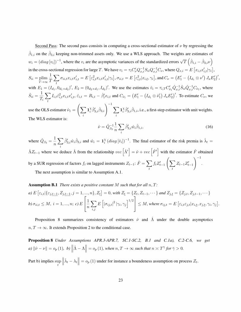
Second Pass: The second pass consists in computing a cross-sectional estimator of ν by regressing the

β1,i on the β3,i keeping non-trimmed assets only. We use a WLS approach. The weights are estimates of

wi = (diag [vi])−1, where the vi are the asymptotic variances of the standardized errors

√T(β1,i − β3,iν

)in the cross-sectional regression for large T . We have vi = τiC

′νQ−1x,iSiiQ

−1x,iCν , whereQx,i = E

[xi,tx

′i,t|γi

],

Sii = plimT→∞

1

T

∑t

σii,txi,tx′i,t = E

[ε2i,txi,tx

′i,t|γi

], σii,t = E

[ε2i,t|xi,t, γi

], andCν =

(E′1 −

(Id1 ⊗ ν ′

)JaE

′2

)′,with E1 = (Id1 , 0d1×d2)′, E2 = (0d2×d1 , Id2)′. We use the estimates vi = τi,TC

′ν1Q

−1x,i SiiQ

−1x,iCν1 , where

Sii =1

Ti

∑t

Ii,tε2i,txi,tx

′i,t, εi,t = Ri,t − β′ixi,t and Cν1 =

(E′1 −

(Id1 ⊗ ν ′1

)JaE

′2

)′. To estimate Cν , we

use the OLS estimator ν1 =

(∑i

1χi β′3,iβ3,i

)−1∑i

1χi β′3,iβ1,i, i.e., a first-step estimator with unit weights.

The WLS estimator is:

ν = Q−1β3

1

n

∑i

β′3,iwiβ1,i, (16)

where Qβ3 =1

n

∑i

β′3,iwiβ3,i and wi = 1χi (diag [vi])−1. The final estimator of the risk premia is λt =

ΛZt−1 where we deduce Λ from the relationship vec[Λ′]

= ν + vec[F ′]

with the estimator F obtained

by a SUR regression of factors ft on lagged instruments Zt−1: F =∑t

ftZ′t−1

(∑t

Zt−1Z′t−1

)−1

.

The next assumption is similar to Assumption A.1.

Assumption B.1 There exists a positive constant M such that for all n, T :

a) E[εi,t|εj,t−1, Zj,t−1, j = 1, ..., n, Zt

]= 0, with Zt = Zt, Zt−1, · · · and Zj,t = Zj,t, Zj,t−1, · · ·

b) σii,t ≤M, i = 1, ..., n; c)E

1

n

∑i,j

E[|σij,t|2 |γi, γj

]1/2

≤M , where σij,t = E[εi,tεj,t|xi,t, xj,t, γi, γj

].

Proposition 8 summarizes consistency of estimators ν and Λ under the double asymptotics

n, T →∞. It extends Proposition 2 to the conditional case.

Proposition 8 Under Assumptions APR.3-APR.7, SC.1-SC.2, B.1 and C.1a), C.2-C.6, we get

a) ‖ν − ν‖ = op (1), b)∥∥∥Λ− Λ

∥∥∥ = op (1), when n, T →∞ such that n T γ for γ > 0.

Part b) implies supt

∥∥∥λt − λt∥∥∥ = op (1) under for instance a boundeness assumption on process Zt.

23

Proposition 9 below gives the large-sample distributions under the double asymptotics

n, T → ∞. It extends Proposition 3 to the conditional case through adequate use of selection matri-

ces. The following assumption is similar to Assumption A.2. We make use of Qβ3 = EG[β′3,iwiβ3,i

],

Qz = E[ZtZ

′t

], Sij = plim

T→∞

1

T

∑t

σij,txi,tx′j,t = E[εi,tεj,txi,tx

′j,t|γi, γj ] and SQ,ij = Q−1

x,iSijQ−1x,j , other-

wise, we keep the same notations as in Section 2.

Assumption B.2 As n, T →∞ such that n T γ for γ ∈ Γ1 ⊂ R+, a)1√n

∑i

τi

[(Q−1

x,iYi,T )⊗ v3,i

]⇒

N (0, Sv3) ,with Yi,T =1√T

∑t

Ii,txi,tεi,t, v3,i = vec[β′3,iwi] and Sv3 = limn→∞

E

1

n

∑i,j

τiτjτij

SQ,ij ⊗ v3,iv′3,j

= plim

n→∞

1

n

∑i,j

τiτjτij

[SQ,ij ⊗ v3,iv′3,j ]; b)

1√T

∑t

ut ⊗ Zt−1 ⇒ N (0,Σu) ,where Σu = E[utu′t ⊗ Zt−1Z

′t−1

]and ut = ft − FZt−1.

Proposition 9 Under Assumptions APR.3-APR.7,SC.1-SC.2,B.1-B.2 and C.1a), C.2-C.6, we have

a)√nT

(ν − ν − 1

TBν

)⇒ N (0,Σν) where Bν = Q−1

β3Jb

1

n

∑i

τi,T vec[E′2Q

−1x,i SiiQ

−1x,iCνwi

]and

Σν =(vec

[C ′ν]⊗Q−1

β3

)′Sv3

(vec

[C ′ν]⊗Q−1

β3

), with Jb =

(vec [Id1 ]′ ⊗ IKp

)(Id1 ⊗ Ja) and

Cν =(E′1 −

(Id1 ⊗ ν ′

)JaE

′2

)′; b)√Tvec

[Λ′ − Λ′

]⇒N (0,ΣΛ) where ΣΛ =

(IK ⊗Q−1

z

)Σu

(IK ⊗Q−1

z

),

when n, T →∞ such that n T γ for γ ∈ Γ1 ∩ (0, 3).

Since λt = ΛZt−1 =(Z ′t−1 ⊗ IK

)Wp,Kvec

[Λ′], part b) implies conditionally on Zt−1 that

√T(λt − λt

)⇒ N

(0,(Z ′t−1 ⊗ IK

)Wp,KΣΛWK,p (Zt−1 ⊗ IK)

).

We can use Proposition 9 to build confidence intervals. It suffices to replace the unknown quantities Qx,

Qz , Qβ3 , Σu and ν by their empirical counterparts. For matrix Sv3 we use the thresholded estimator Sij as

in Section 2.4. Then we can extend Proposition 4 to the conditional case under Assumptions B.1-B.2, A.3,

A.4 and C.1-C.6.

Since Equation (14) corresponds to the asset pricing restriction (3), the null hypothesis of correct speci-

fication of the conditional model is

H0 : there exists ν ∈ RpK such that β1(γ) = β3(γ)ν, with vec[β3(γ)′

]= Jaβ2(γ),

for almost all γ ∈ [0, 1].

24

UnderH0, we have EG[(β1,i − β3,iν)′ (β1,i − β3,iν)

]= 0. The alternative hypothesis is

H1 : infν∈RdK

EG[(β1,i − β3,iν)′ (β1,i − β3,iν)

]> 0.

As in Section 2.5, we build the SSR Qe =1

n

∑i

e′iwiei, with ei = β1,i − β3,iν = C ′ν βi and

the statistic ξnT = T√n

(Qe −

1

TBξ

), where Bξ = d1.

Assumption B.3 For n, T → ∞ such that n T γ for γ ∈ Γ2 ⊂ Γ1, we have1√n

∑i

τ2i

[(Q−1x,i ⊗Q

−1x,i

)(Yi,T ⊗ Yi,T − vec [Sii,T ])

]⊗ vec[wi]⇒ N (0,Ω), where the asymptotic vari-

ance matrix is:

Ω = limn→∞

E

1

n

∑i,j

τ2i τ

2j

τ2ij

[SQ,ij ⊗ SQ,ij + (SQ,ij ⊗ SQ,ij)Wd]⊗(vec[wi]vec[wj ]

′)= plim

n→∞

1

n

∑i,j

τ2i τ

2j

τ2ij

[SQ,ij ⊗ SQ,ij + (SQ,ij ⊗ SQ,ij)Wd]⊗(vec[wi]vec[wj ]

′) .Proposition 10 Under H0 and Assumptions APR.3-APR.7, SC.1-SC.2, B.1-B.2, A.3, A.4 and C.1-C.6, we

have Σ−1/2ξ ξnT ⇒ N (0, 1) ,where Σξ = 2

1

n

∑i,j

τ2i,T τ

2j,T

τ2ij,T

tr[wi

(C ′νQ

−1x,i SijQ

−1x,jCν

)wj

(C ′νQ

−1x,jSjiQ

−1x,iCν

)]as n, T →∞ such that n T γ for γ ∈ Γ2 ∩

(0,min

2η, η

1− q2δ

).

UnderH1, we have ξp→ +∞, as in Proposition 6.

As in Section 2.5, the null hypothesis when the factors are tradable assets becomes:

H0 : β1(γ) = 0 for almost all γ ∈ [0, 1],

against the alternative hypothesis

H1 : EG[β′1,iβ1,i

]> 0.

We only have to substitute Qa =1

n

∑i

β′1,iwiβ1,i for Qe, and E1 = (Id1 : 0)′ for Cν . This gives an exten-

sion of Gibbons, Ross and Shanken (1989) to the conditional case and with double asymptotics. Implement-

ing the original Gibbons, Ross and Shanken (1989) test, which uses a weighting matrix corresponding to an

inverted estimated covariance matrix, becomes quickly problematic; each β1,i is of dimension d1 × 1, and

25

the inverted matrix is of dimension nd1×nd1. We expect to compensate the potential loss of power induced

by a diagonal weighting thanks to the large number nd1 of restrictions. Our preliminary unreported Monte

Carlo simulations show that the test exhibits good power properties for a couple of hundreds of assets.

4 Empirical results

4.1 Asset pricing model and data description

Our baseline asset pricing model is a four-factor model with ft = (rm,t, rsmb,t, rhml,t, rmom,t)′ where rm,t is

the month t excess return on CRSP NYSE/AMEX/Nasdaq value-weighted market portfolio over the risk free

rate (proxied by the monthly 30-day T-bill beginning-of-month yield), and rsmb,t, rhml,t and rmom,t are the

month t returns on zero-investment factor-mimicking portfolios for size, book-to-market, and momentum

(see Fama and French (1993), Jegadeesh and Titman (1993), Carhart (1997)). To account for time-varying

alphas, betas and risk premia, we use a specification based on two common variables and two firm-level

variables. We take the instruments Zt = (1, Z∗t′)′, where bivariate vector Z∗t includes the term spread,

proxied by the difference between yields on 10-year Treasury and three-month T-bill, and the default spread,

proxied by the yield difference between Moody’s Baa-rated and Aaa-rated corporate bonds. We take Zi,t

as a bivariate vector made of the market capitalization and the book-to-market equity of firm i. We refer

to Avramov and Chordia (2006) for convincing theoretical and empirical arguments in favor of the chosen

conditional specification. The vector xi,t is of dimension d = 32. The firm characteristics are computed as

in the appendix of Fama and French (2008) from Compustat. We use monthly stock returns data provided by

CRSP and we exclude financial firms (Standard Industrial Classification Codes between 6000 and 6999) as

in Fama and French (2008). The dataset after matching CRSP and Compustat contents comprises n = 9, 936

stocks and covers the period from July 1964 to December 2009 with T = 546. For comparison purposes

with a standard methodology for small n, we consider the 25 and 100 Fama-French (FF) portfolios as base

assets. We have downloaded the time series of factors, portfolios and portfolio characteristics from the

website of Kenneth French.

26

4.2 Estimation results

We first present unconditional estimates before looking at the path of the time-varying estimates. We use

χ1,T = 15 and χ2,T = 546/12 for the unconditional estimation and χ1,T = 15 and χ2,T = 546/36 for the

conditional estimation. In the reported results for the four-factors model, we denote by nχ the dimension of

the cross-section after trimming. We use a data-driven threshold selected by cross-validation as in Bickel and

Levina (2008). Table 1 gathers the estimated annual risk premia for the following unconditional models:

the four-factor model, the Fama-French model, and the CAPM. In Table 2, we display the estimates of

the components of ν. When n is large, we use bias-corrected estimates for λ and ν. When n is small,

we use asymptotics for fixed n and T → ∞. The estimated risk premia for the market factor are of

the same magnitude and all positive across the three universes of assets and the three models. The 95%

confidence intervals are larger by construction for fixed n, and they often contain the interval for large n.

For the four-factor model and the individual stocks the size factor is positively remunerated (2.91%) and it

is not significantly different from zero. The value factor commands a significant negative reward (-4.55%).

Phalippou (2007) obtained a similar result, indeed he got a growth premium when portofolios are built

on stocks with a high institutional ownership. The momentum factor is largely remunerated (7.34%) and

significantly different from zero. For the 25 and 100 FF portfolios we observe that the size factor is not

significantly positively remunerated while the value factor is significantly positively remunerated (4.81%

and 5.11%). The momentum factor bears a significant positive reward (34.03% and 17.29%). The large, but

imprecise, estimate for the momentum premium when n = 25 and n = 100 comes from the estimate for

νmom (25.40% and 8.66% ) that is much larger and less accurate than the estimates for νm, νsmb and νhml

(0.85%, -0.26%, 0.03%, and 0.55%, 0.01%, 0.33%). Moreover, while for portfolios the estimates of νm,

νsmb and νhml are statistically not significant, for individual stocks these estimates are statistically different

from zero. In particular, the estimate of νhml is large and negative, which explains the negative estimate on

the value premium displayed in Table 1.

As showed in Figure 1, a potential explanation of the discrepancies revealed in Tables 1 and 2 between

individual stocks and portfolios is the much larger heterogeneity of the factor loadings for the former. The

portfolio betas are all concentrated in the middle of the cross-sectional distribution obtained from the indi-

vidual stocks. Creating portfolios distorts information by shrinking the dispersion of betas. The estimation

27

results for the momentum factor exemplify the problems related to a small number of portfolios exhibiting

a tight factor structure (Lewellen, Nagel and Shanken (2010)). For λm, λsmb, and λhml, we obtain similar

inferential results when we consider the Fama-French model. Our point estimates for λm, λsmb and λhml,

for large n agree with Ang, Liu and Schwarz (2008). Our point estimates and confidence intervals for λm,

λsmb and λhml, agree with the results reported by Shanken and Zhou (2007) for the 25 portfolios.

Figure 2 plots the estimated time-varying path of the four risk premia from the individual stocks. We

also plot the unconditional estimates and the average lambda over time. The discrepancy between the uncon-

ditional estimate and the average over time is explained by a well-known bias coming from market-timing

and volatility-timing (Jagannathan and Wang (1996), Lewellen and Nagel (2006), Boguth, Carlson, Fisher

and Simutin (2010)). The risk premia for the market, size and value factors feature a counter-cyclical pat-

tern. Indeed, these risk premia increase during economic contractions and decrease during economic booms.

Gomes, Kogan and Zhang (2003) and Zhang (2005) construct equilibrium models exhibiting a countercycli-

cal behavior in size and book-to-market effects. On the contrary, the risk premium for momentum factor

is pro-cyclical. Furthermore, conditional estimates of the value premium take stable and positive values.

They are not significantly different from zero during economic booms. The conditional estimates of the size

premium are most of the time slightly positive, and not significantly different from zero.

Figure 3 plots the estimated time-varying path of the four risk premia from the 25 portfolios. We also plot

the unconditional estimates and the average lambda over time. The discrepancy between the unconditional

estimate and the averages over time is also observed for n = 25. The conditional point estimates for

λmom,t are larger and more imprecise than the unconditional estimate in Table 1. Indeed, the pointwise

confidence intervals contain the confidence interval of the unconditional estimate for λmom. Finally, by

comparing Figures 2 and 3, we observe that the patterns of risk premia look similar except for the book-to-

market factor. Indeed, the risk premium for the value effect estimated from the 25 portfolios is pro-cyclical,

contradicting the counter-cyclical behavior predicted by finance theory. By comparing Figures 3 and 4, we

observe that increasing the number of portfolios to 100 does not help in reconciling the discrepancy.

28

4.3 Specification test results

As already mentioned Figure 1 shows that the 25 FF portfolios all have four-factor market and momentum

betas close to one and zero, respectively, so the model can be thought as a two-factor model consisting of

smb and hml for the purposes of explaining cross-sectional variation in expected returns. For the 100 FF

portfolios the dispersion around one and zero is slightly larger. As depicted in Figure 1 by Lewellen, Nagel

and Shanken (2010), this empirical concentration implies that it is easy to get artificially large estimates ρ2

of the cross-sectional R2 for three- and four-factor models. On the contrary, the observed heterogeneity in

the betas coming from the individual stocks impedes this. This suggests that it is much less easy to find

factors that explain the cross-sectional variation of expected returns on individual stocks than on portfolios.

Reporting large ρ2, or small SSR Qe, when n is large, is much more impressive than when n is small.

Table 2 gathers specification test results for unconditional factor models. As already mentioned, when

n is large, we prefer working with test statistics based on the SSR Qe instead of ρ2 since the population R2

is not well-defined with tradable factors under the null hypothesis of well-specification (its denominator is

zero). For the individual stocks, we compute the test statistic Σ−1/2ξ ξnT as well as its associated p-value. For

the 25 and 100 FF portfolios, we compute weighted test statistics (Gibbons, Ross and Shanken (1989)) as

well as their associated p-value. We do similarly for the test statistics relying on the alphas a. As expected

the rejection of the well specification is strong on the individual stocks. This suggests that the unconditional

models do not describe the behavior of individual stocks. For the 25 portfolios, the Gibbons-Ross-Shanken

test statistic rejects the well specification for the CAPM and the three-factor model. The four-factor model

is not rejected at 1% level, but it is rejected at 5% level.

4.4 Cost of equity

The results in Section 3 can be used for estimation and inference on the cost of equity in conditional factor

models. We can estimate the time varying cost of equity CEi,t = rf,t + b′i,tλt of firm i with CEi,t =

rf,t + b′i,tλt, where rf,t is the risk-free rate. We have (see Appendix 3)

√T(CEi,t − CEi,t

)= ψ′i,tE

′2

√T(βi − βi

)+(Z ′t−1 ⊗ b′i,t

)Wp,K

√Tvec

[Λ′ − Λ′

]+ op (1) , (17)

29

where ψi,t =(λ′t ⊗ Z ′t−1, λ

′t ⊗ Z ′i,t−1

)′. Standard results on OLS imply that estimator βi is asymptotically

normal,√T(βi − βi

)⇒ N

(0, τ2

i Q−1x,iSiiQ

−1x,i

), and independent of estimator Λ. Then, from Proposition

7 we deduce that√T(CEi,t − CEi,t

)⇒ N

(0,ΣCEi,t

), conditionally on Zt−1, where

ΣCEi,t = τ2i ψ′i,tE

′2Q−1x,iSiiQ

−1x,iE2ψi,t +

(Z ′t−1 ⊗ b′i,t

)Wp,KΣΛWK,p (Zt−1 ⊗ bi,t) .

Figure 5 plots the path of the estimated annualized costs of equity for Ford Motor, Disney, Motorola and

Sony. The cost of equity has risen tremendously during the recent subprime crisis.

30

References

D. W. K. Andrews. Cross-section regression with common shocks. Econometrica, 73(5):1551–1585, 2005.

D. W. K. Andrews and J. C. Monahan. An improved heteroskedasticity and autocorrelation consistent

covariance matrix estimator. Econometrica, 60(4):953–966, 1992.

A. Ang, J. Liu, and K. Schwarz. Using individual stocks or portfolios in tests of factor models. Working

Paper, 2008.

D. Avramov and T. Chordia. Asset pricing models and financial market anomalies. The Review of Financial

Studies, 19(3):1000–1040, 2006.

J. Bai. Inferential theory for factor models of large dimensions. Econometrica, 71(1):135–171, 2003.

J. Bai. Panel data models with interactive fixed effects. Econometrica, 77(4):1229–1279, 2009.

J. Bai and S. Ng. Determining the number of factors in approximate factor models. Econometrica, 70(1):

191–221, 2002.

J. Bai and S. Ng. Confidence intervals for diffusion index forecasts and inference for factor-augmented

regressions. Econometrica, 74(4):1133–1150, 2006.

D.A. Belsley, E. Kuh, and R.E. Welsch. Regression diagnostics - Identifying influential data and sources of

collinearity. John Wiley & Sons, 2004.

J. B. Berk. Sorting out sorts. Journal of Finance, 55(1):407–427, 2000.

P. J. Bickel and E. Levina. Covariance regularization by thresholding. The Annals of Statistics, 36(6):

2577–2604, 2008.

P. Billingsley. Probability and measure, 3rd Edition. John Wiley and Sons, New York, 1995.

F. Black, M. Jensen, and M. Scholes. The Capital Asset Pricing Model: Some Empirical Findings In Jensen,

M.C. (Ed.), Studies in the Theory of Capital Markets. Praeger, New York. Praeger, New York, 1972.

31

O. Boguth, M. Carlson, A. Fisher, and M. Simutin. Conditional risk and performance evaluation: volatility

timing, overconditioning, and new estimates of momentum alphas. Journal of Financial Economics,

forthcoming, 2010.

D. Bosq. Nonparametric Statistics for Stochastic Processes. Springer-Verlag New York, 1998.

S. J. Brown, W. N. Goetzmann, and S. A. Ross. Survival. The Journal of Finance, 50(3):853–873, 1995.

M. Carhart. On persistence of mutual fund performance. Journal of Finance, 52(1):57–82, 1997.

G. Chamberlain. Funds, factors, and diversification in arbitrage pricing models. Econometrica, 51(5):

1305–1323, 1983.

G. Chamberlain and M. Rothschild. Arbitrage, factor structure, and mean-variance analysis on large asset

markets. Econometrica, 51(5):1281–1304, 1983.

J. H. Cochrane. A cross-sectional test of an investment-based asset pricing model. Journal of Political

Economy, 104(3):572–621, 1996.

G. Connor and R. A. Korajczyk. Estimating pervasive economic factors with missing observations. Working

Paper No. 34, Department of Finance, Northwestern University, 1987.

G. Connor and R. A. Korajczyk. An intertemporal equilibrium beta pricing model. The Review of Financial

Studies, 2(3):373–392, 1989.

G. Connor, M. Hagmann, and O. Linton. Efficient estimation of a semiparametric characteristic-based factor

model of security returns. Econometrica, forthcoming, 2011.

J. Conrad, M. Cooper, and G. Kaul. Value versus glamour. The Journal of Finance, 58(5):1969–1995, 2003.

J. Doob. Stochastic processes. John Wiley and sons, New York, 1953.

D. Duffie. Dynamic asset pricing theory, 3rd Edition. Princeton University Press, Princeton, 2001.

N. El Karoui. Operator norm consistent estimation of large dimensional sparce covariance matrices. Annals

of Statistics, 36(6):2717–2756, 2008.

32

E. F. Fama and K. R. French. Common risk factors in the returns on stocks and bonds. Journal of Financial

Economics, 33(1):3–56, 1993.

E. F. Fama and K. R. French. Industry costs of equity. Journal of Financial Economics, 43(2):153–193,

1997.

E. F. Fama and K. R. French. Dissecting anomalies. The Jounal of Finance, 63(4):1653–1678, 2008.

E. F. Fama and J. D. MacBeth. Risk, return, and equilibrium: Empirical tests. Journal of Political Economy,

81(3):607–36, 1973.

J. Fan, Y. Liao, and M. Mincheva. High dimensional covariance matrix estimation in approximate factor

structure. Princeton University Working Paper, 2011.

W. E. Ferson and C. R. Harvey. The variation of economic risk premiums. Journal of Political Economy,

99(2):385–415, 1991.

W. E. Ferson and C. R. Harvey. Conditioning variables and the cross section of stock returns. Journal of

Finance, 54(4):1325–1360, 1999.

W. E. Ferson and R. W. Schadt. Measuring fund strategy and performance in changing economic conditions.

Journal of Finance, 51(2):425–61, 1996.

M. Forni, M. Hallin, M. Lippi, and L. Reichlin. The generalized dynamic factor model: identification and

estimation. The Review of Economics and Statistics, 82(4):540–54, 2000.

M. Forni, M. Hallin, M. Lippi, and L. Reichlin. The generalized dynamic factor model: consistency and

rates. Journal of Econometrics, 119(2):231–55, 2004.

M. Forni, M. Hallin, M. Lippi, and L. Reichlin. The generalized dynamic factor model one-sided estimation

and forecasting. Journal of the American Statistical Association, 100(4):830–40, 2005.

E. Ghysels. On stable factor structures in the pricing of risk: do time-varying betas help or hurt? Jounal of

Finance, 53(2):549–573, 1998.

33

R. Gibbons, S. A. Ross, and J. Shanken. A test of the efficiency of a given portfolio. Econometrica, 57(5):

1121–1152, 1989.

J. Gomes, L. Kogan, and L. Zhang. Equilibrium cross section of returns. Journal of Political Economy, 111

(4):693–732, 2003.

C. Gourieroux, A. Monfort, and Trognon A. Pseudo maximum likelihood methods: theory. Econometrica,

52(3):681–700, 1984.

W. Greene. Econometric Analysis, 6th ed. Prentice Hall, 2008.

J. Hahn and G. Kuersteiner. Asymptotically unbiased inference for a dynamic panel model with fixed effects

when both n and t are large. Econometrica., 70(4):1639–1657, 2002.

J. Hahn and W. Newey. Jackknife and analytical bias reduction for nonlinear panel models. Econometrica,

72(4):1295–1319, 2004.

L. P. Hansen and S. F. Richard. The role of conditioning information in deducing testable restrictions implied

by dynamic asset pricing models. Econometrica, 55(3):587–613, 1987.

J. Heckman. Sample selection bias as a specification error. Econometrica, 47(1):153–161, 1979.

R. Jagannathan and Z. Wang. The conditional capm and the cross-section of expected returns. Journal of

Finance, 51(1):3–53, 1996.

R. Jagannathan and Z. Wang. An asymptotic theory for estimating beta-pricing models using cross-sectional

regression. Journal of Finance, 53(4):1285–1309, 1998.

R Jagannathan, G. Skoulakis, and Z. Wang. The analysis of the cross section of security returns. Handbook

of Financial Econometrics, 2:73–134, North-Holland, 2009.

N. Jegadeesh and S. Titman. Returns to buying winners and selling losers: implications for stock market

efficiency. Journal of Finance, 48(1):65–91, 1993.

R. Kan, C. Robotti, and J. Shanken. Pricing model performance and the two-pass cross-sectional regression

methodology. Working Paper, 2009.

34

S. Kandel and S. Stambaugh. Portfolio inefficiency and the cross-section of expected returns. The Journal

of Finance, 50(1):157–184, 1995.

T. Lancaster. The incidental parameter problem since 1948. Journal of Econometrics, 95(2):391–413, 2000.

M. Lettau and S. Ludvigson. Consumption, aggregate wealth, and expected stock returns. Journal of

Finance, 56(3):815–849, 2001.

J. Lewellen and S. Nagel. The conditional capm does not explain asset-pricing anomalies. Journal of

Financial Economics, 82(2):289–314, 2006.

J. Lewellen, S. Nagel, and J. Shanken. A skeptical appraisal of asset-pricing tests. Journal of Financial

Economics, 96(2):175–194, 2010.

J. Lintner. The valuation of risk assets and the selection of risky investments in stock portfolios and capital

budgets. The Review of Economics and Statistics, 47(1):13–37, 1965.

R. H. Litzenberger and K. Ramaswamy. The effect of personal taxes and dividends on capital asset prices:

Theory and empirical evidence. Journal of Financial Economics, 7(2):163–195, 1979.

A. W. Lo and A. C. MacKinlay. Data-snooping biases in tests of financial asset pricing models. The Review

of Financial Studies, 3(3):431–67, 1990.

S. Ludvigson. Advances in consumption-based asset pricing: Empirical tests. Handbook of the Economics

of Finance vol. 2, edited by George Constantinides, Milton Harris and Rene Stulz, forthcoming, 2011.

S. Ludvigson and S. Ng. The empirical risk-return relation: a factor analysis approach. Journal of Financial

Economics, 83:171–222, 2007.

S. Ludvigson and S. Ng. Macro factors in bond risk premia. The Review of Financial Studies, 22(12):

5027–5067, 2009.

J. R. Magnus and H. Neudecker. Matrix Differential Calculus with Applications in Statistics and Economet-

rics. John Wiley & Sons, 2007.

35

W. K. Newey and K. D. West. Automatic lag selection in covariance matrix estimation. Review of Economic

Studies, 61(4):631–653, 1994.

J. Neyman and E.L. Scott. Consistent estimation from partially consistent observations. Econometrica, 16

(1):1–32, 1948.

M. H. Pesaran. Estimation and inference in large heterogeneous panels with a multifactor error structure.

Econometrica, 74(4):967–1012, 2006.

M. H. Pesaran and T. Yamagata. Testing slope homogeneity in large panels. Journal of Econometrics, 142

(1):50–93, 2008.

M. Petersen. Estimating standard errors in finance panel data sets: comparing approaches. The Review of

Financial Studies, 22(1):451–480, 2008.

R. Petkova and L. Zhang. Is value riskier than growth? Journal of Financial Economics, 78(1):187–202,

2005.

L. Phalippou. Can risk-based theories explain the value premium? Review of Finance, 11(2):143–166,

2007.

S. A. Ross. The arbitrage theory of capital asset pricing. Journal of Economic Theory, 13(3):341–360, 1976.

S. A. Ross. A simple approach to the valuation of risky streams. Journal of Business, 51(3):453–476, 1978.

D. B. Rubin. Inference and missing data. Biometrika, 63(3):581–592, 1976.

J. Shanken. The arbitrage pricing theory: is it testable? Journal of Finance, 37(5):1129–1140, 1982.

J. Shanken. Multivariate tests of the zero-beta capm. Journal of Financial Economics, 14(3):327–348, 1985.

J. Shanken. Intertemporal asset pricing: An empirical investigation. Journal of Econometrics, 45(1-2):

99–120, 1990.

J. Shanken. On the estimation of beta-pricing models. The Review of Financial Studies, 5(1):1–33, 1992.

36

J. Shanken and G. Zhou. Estimating and testing beta pricing models: Alternative methods and their perfor-

mance in simulations. Journal of Financial Economics, 84(1):40–86, 2007.

W. Sharpe. Capital asset prices: A theory of market equilibrium under conditions of risk. Journal of Finance,

19(3):425–442, 1964.

J. H. Stock and M. W. Watson. Forecasting using principal components from a large number of predictors.

Journal of American Statistical Association, 97(460):1167–1179, 2002 a.

J. H. Stock and M. W. Watson. Macroeconomic forecasting using diffusion indexes. Journal of Business

and Economic Statistics, 20(2):147–62, 2002 b.

W. Stout. Almost sure convergence. Academic Press, New York, 1974.

H. White. Maximum likelihood estimation of misspecified models. Econometrica, 50(1):1–25, 1982.

J.M. Wooldridge. Econometric Analysis of Cross Section and Panel Data. MIT Press, 2002.

L. Zhang. The value premium. Jounal of Finance, 60(1):67–103, 2005.

37

Figure 1: Distribution of the factor loadings

−25

−20

−15

−10

−5

0

5

10

15

20

25

βm βsmb βhml βmom

The figure displays box-plots for the distribution of factor loadings βm, βsmb, βhml and βmom. The factor

loadings are estimated by running the time-series OLS regression in equation (2) for n = 9, 936 from

1964/07 to 2009/12. Moreover, next to each box-plot we report the estimated factor loadings for the 25 and

100 Fama-French portfolios (circles and triangles, respectively).

38

Figu

re2:

Path

ofes

timat

edan

nual

ized

risk

prem

iaw

ithn

=9,

936

6570

7580

8590

9500

0510

−40

−200204060

λm

,t

6570

7580

8590

9500

0510

−40

−2002040

λsm

b,t

6570

7580

8590

9500

0510

−40

−2002040

λhm

l,t

6570

7580

8590

9500

0510

−10

0

−50050100

λm

om

,t

The

figur

epl

ots

the

path

ofes

timat

edan

nual

ized

risk

prem

iaλm

,λsm

b,λ

hml

andλmom

and

thei

rpo

intw

ise

confi

denc

ein

terv

als

at

95%

prob

abili

tyle

vel.

We

also

repo

rtth

eun

cond

ition

ales

timat

e(d

ashe

dho

rizo

ntal

line)

and

the

aver

age

cond

ition

ales

timat

e(s

olid

hori

zont

allin

e).

We

cons

ider

alls

tock

s(n

=9,

926

andnχ

=2,

612)

asba

seas

sets

.T

heve

rtic

alsh

aded

area

sde

note

rece

ssio

ns

dete

rmin

edby

the

Nat

iona

lBur

eau

ofE

cono

mic

Res

earc

h(N

BE

R).

The

rece

ssio

nsst

arta

tthe

peak

ofa

busi

ness

cycl

ean

den

dat

the

trou

gh.

39

Figu

re3:

Path

ofes

timat

edan

nual

ized

risk

prem

iaw

ithn

=25

The

figur

epl

ots

the

path

ofes

timat

edan

nual

ized

risk

prem

iaλm

,λsm

b,λ

hml

andλmom

and

thei

rpo

intw

ise

confi

denc

ein

terv

als

at

95%

prob

abili

tyle

vel.

We

also

repo

rtth

eun

cond

ition

ales

timat

e(d

ashe

dho

rizo

ntal

line)

and

the

aver

age

cond

ition

ales

timat

e(s

olid

hori

zont

allin

e).T

heve

rtic

alsh

aded

area

sde

note

rece

ssio

nsde

term

ined

byth

eN

atio

nalB

urea

uof

Eco

nom

icR

esea

rch

(NB

ER

).

40

Figu

re4:

Path

ofes

timat

edan

nual

ized

risk

prem

iaw

ithn

=10

0

The

figur

epl

ots

the

path

ofes

timat

edan

nual

ized

risk

prem

iaλm

,λsm

b,λ

hml

andλmom

and

thei

rpo

intw

ise

confi

denc

ein

terv

als

at

95%

prob

abili

tyle

vel.

We

also

repo

rtth

eun

cond

ition

ales

timat

e(d

ashe

dho

rizo

ntal

line)

and

the

aver

age

cond

ition

ales

timat

e(s

olid

hori

zont

allin

e).T

heve

rtic

alsh

aded

area

sde

note

rece

ssio

nsde

term

ined

byth

eN

atio

nalB

urea

uof

Eco

nom

icR

esea

rch

(NB

ER

).

41

Figu

re5:

Path

ofes

timat

edan

nual

ized

cost

sofe

quity

6570

7580

8590

9500

0510

−40

−20020406080100

120

CE

ofFord

Motor(F

)

6570

7580

8590

9500

0510

−40

−20020406080100

120

CE

ofDisney

(DIS)

6570

7580

8590

9500

0510

−40

−20020406080100

120

CE

ofMotorola

(MSI)

6570

7580

8590

9500

0510

−40

−20020406080100

120

CE

ofSony(SNE)

The

figur

epl

otst

hepa

thof

estim

ated

annu

aliz

edco

stof

equi

tiesf

orFo

rdM

otor

,Dis

ney

Wal

t,M

otor

ola

and

Sony

and

thei

rpoi

ntw

ise

confi

denc

ein

terv

als

at95

%pr

obab

ility

leve

l.W

eal

sore

port

the

unco

nditi

onal

estim

ate

(das

hed

hori

zont

allin

e)an

dth

eav

erag

e

cond

ition

ales

timat

e(s

olid

hori

zont

allin

e).

The

vert

ical

shad

edar

eas

deno

tere

cess

ions

dete

rmin

ated

byth

eN

atio

nal

Bur

eau

of

Eco

nom

icR

esea

rch

(NB

ER

).

42

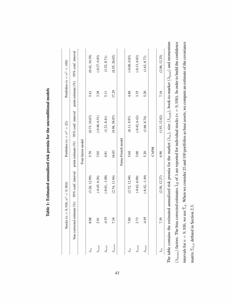
Tabl

e1:

Est

imat

edan

nual

ized

risk

prem

iafo

rth

eun

cond

ition

alm

odel

s

Stoc

ks(n

=9,936

,nχ=

9,902

)Po

rtfo

lios

(n=nχ=

25

)Po

rtfo

lios

(n=nχ=

100

)

bias

corr

ecte

des

timat

e(%

)95

%co

nf.i

nter

val

poin

test

imat

e(%

)95

%co

nf.i

nter

val

poin

test

imat

e(%

)95

%co

nf.i

nter

val

Four

-fac

torm

odel

λm

8.08

(3.2

0,12

.99)

5.70

(0.7

3,10

.67)

5.41

(0.4

2,10

.39)

λsmb

2.91

(-0.

45,6

.26)

3.02

(-0.

48,6

.51)

3.28

(-0.

27,6

.83)

λhml

-4.5

5(-

8.01

,-1.

08)

4.81

(1.2

1,8.

41)

5.11

(1.5

2,8.

71)

λmom

7.34

(2.7

4,11

.94)

34.0

3(9

.98,

58.0

7)17

.29

(8.5

5,26

.03)

Fam

a-Fr

ench

mod

el

λm

7.60

(2.7

2,12

.49)

5.04

(0.1

1,9.

97)

4.88

(-0.

08,0

.83)

λsmb

2.73

(-0.

62,6

.09)

3.00

(-0.

42,6

.42)

3.35

(-0.

13,6

.83)

λhml

-4.9

5(-

8.42

,-1.

49)

5.20

(1.6

6,8.

74)

5.20

(1.6

3,8.

77)

CA

PM

λm

7.39

(2.5

0,12

.27)

6.98

(1.9

3,12

.02)

7.16

(2.0

6,12

.25)

The

tabl

eco

ntai

nsth

ees

timat

edan

nual

ized

risk

prem

iafo

rth

em

arke

t(λm

),si

ze(λsm

b),

book

-to-

mar

ket(λhml)

and

mom

entu

m

(λmom

)fa

ctor

s.T

hebi

asco

rrec

ted

estim

atesλB

ofλ

are

repo

rted

fori

ndiv

idua

lsto

cks

(n=

9,93

6).

Inor

dert

obu

ildth

eco

nfide

nce

inte

rval

sforn

=9,

936,w

eus

eΣf.W

hen

we

cons

ider

25an

d10

0po

rtfo

liosa

sbas

eas

sets

,we

com

pute

anes

timat

eof

the

cova

rian

ce

mat

rix

Σλ,n

defin

edin

Sect

ion

2.3.

43

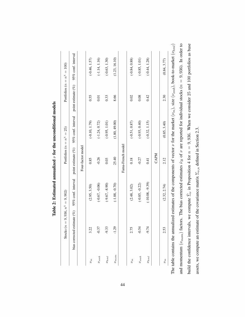
Tabl

e2:

Est

imat

edan

nual

izedν

for

the

unco

nditi

onal

mod

els

Stoc

ks(n

=9,936

,nχ=

9,902

)Po

rtfo

lios

(n=nχ=

25

)Po

rtfo

lios

(n=nχ=

100

)

bias

corr

ecte

des

timat

e(%

)95

%co

nf.i

nter

val

poin

test

imat

e(%

)95

%co

nf.i

nter

val

poin

test

imat

e(%

)95

%co

nf.i

nter

val

Four

-fac

torm

odel

νm

3.22

(2.9

5,3.

50)

0.85

(-0.

10,1

.79)

0.55

(-0.

46,1

.57)

νsmb

-0.3

7(-

0.67

,-0.

06)

-0.2

6(-

1.24

,0.7

2)0.

01(-

1.14

,1.1

6)

νhml

-9.3

3(-

9.67

,-8.

90)

0.03

(-0.

95,1

.01)

0.33

(-0.

63,1

.30)

νmom

-1.2

9(-

1.88

,-0.

70)

25.4

0(1

.80,

49.0

0)8.

66(1

.23,

16.1

0)

Fam

a-Fr

ench

mod

el

νm

2.75

(2.4

8,3.

02)

0.18

(-0.

51,0

.87)

0.02

(-0.

84,0

.88)

νsmb

-0.5

4(-

0.85

,-0.

22)

-0.2

7(-

0.93

,0.4

0)0.

08(-

0.85

,1.0

1)

νhml

-9.7

4(-

10.0

8,-9

.39)

0.41

(-0.

32,1

.15)

0.42

(-0.

44,1

.28)

CA

PM

νm

2.53

(2.3

2,2.

74)

2.12

(0.8

5,3.

40)

2.30

(0.8

4,3.

77)

The

tabl

eco

ntai

nsth

ean

nual

ized

estim

ates

ofth

eco

mpo

nent

sof

vect

orν

fort

hem

arke

t(ν m

),si

ze(νsm

b),

book

-to-

mar

ket(ν hml)

and

mom

entu

m(νmom

)fa

ctor

s.T

hebi

asco

rrec

ted

estim

atesν B

ofν

are

repo

rted

for

indi

vidu

alst

ocks

(n=

9,9

36).

Inor

der

to

build

the

confi

denc

ein

terv

als,

we

com

pute

Σν

inPr

opos

ition

4fo

rn

=9,9

36.

Whe

nw

eco

nsid

er25

and

100

port

folio

sas

base

asse

ts,w

eco

mpu

tean

estim

ate

ofth

eco

vari

ance

mat

rix

Σν,n

defin

edin

Sect

ion

2.3.

44

Tabl

e3:

Spec

ifica

tion

test

resu

ltsfo

rth

eun

cond

ition

alm

odel

s

Test

stat

istic

base

donQe,H

0:a=b′ν

Test

stat

istic

base

donQa

,H0:a=

0

Stoc

ks(n

=9,936

)Po

rtfo

lios

(n=

25

)Po

rtfo

lios

(n=

100

)St

ocks

(n=

9,936

)Po

rtfo

lios

(n=

25

)Po

rtfo

lios

(n=

100

)

Four

-fac

torm

odel

Test

stat

istic

22.9

551

35.2

231

253.

2575

43.2

804

74.9

100

263.

3395

p-va

lue

0.00

000.

0267

0.00

000.

0000

0.00

000.

0000

Fam

a-Fr

ench

mod

el

Test

stat

istic

20.8

816

83.6

846

253.

9652

40.2

845

87.3

767

270.

7899

p-va

lue

0.00

000.

0000

0.00

000.

0000

0.00

000.

0000

CA

PM

Test

stat

istic

22.3

152

110.

8368

276.

3679

26.1

799

111.

6735

278.

3949

p-va

lue

0.00

000.

0000

0.00

000.

0000

0.00

000.

0000

The

test

stat

istic

Σ−

1/2

ξξ nT

defin

edin

Prop

ositi

on5

isco

mpu

ted

forn

=9,

936.F

orn

=25

andn

=10

0,th

ete

stst

atis

ticTe′

Ω−

1e

isre

port

ed.T

hete

stst

atis

ticTa′ Ω−

1a

isal

soco

mpu

ted.

The

tabl

ere

port

sth

ep-

valu

es,r

espe

ctiv

ely.

45

Appendix 1: Regularity conditions

In this Appendix, we list and comment the additional assumptions used to derive the large sample properties

of the estimators and test statistics. For unconditional models, we use Assumptions C.1-C.5 below with

xt = (1, f ′t)′.

Assumption C.1 There exists constants η, η ∈ (0, 1] and C1, C2, C3, C4 > 0 such that for all δ > 0 and

T ∈ N we have:

a) P

[∥∥∥∥∥ 1

T

∑t

(xtx′t − E

[xtx′t

])∥∥∥∥∥ ≥ δ]≤ C1T exp

−C2δ

2T η

+ C3δ−1 exp

−C4T

η.

Furthermore, for all δ > 0, T ∈ N, and 1 ≤ k, l,m ≤ K + 1, the same upper bound holds for:

b) supγ∈[0,1]

P

[∥∥∥∥∥ 1

T

∑t

It(γ)(xtx′t − E

[xtx′t

])∥∥∥∥∥ ≥ δ]

;

c) supγ∈[0,1]

P

[∥∥∥∥∥ 1

T

∑t

It(γ)xtεt(γ)

∥∥∥∥∥ ≥ δ]

;

d) supγ,γ′∈[0,1]

P

[∥∥∥∥∥ 1

T

∑t

It(γ)It(γ′)(εt(γ)εt(γ

′)xtx′t − E

[εt(γ)εt(γ

′)xtx′t

])∥∥∥∥∥ ≥ δ]

;

e) supγ,γ′∈[0,1]

P

[∣∣∣∣∣ 1

T

∑t

It(γ)It(γ′)xk,txl,txm,tεt(γ)

∣∣∣∣∣ ≥ δ]

.

Assumption C.2 There exists c > 0 such that supγ∈[0,1]

E

∥∥∥∥∥ 1

T

∑t

It(γ)(xtx′t − E[xtx

′t])∥∥∥∥∥

4 = O(T−c).

Assumption C.3 a) There exists a constantM such that ‖xt‖ ≤M , P -a.s.. Moreover, b) supγ∈[0,1]

‖β(γ)‖ <∞

and c) infγ∈[0,1]

E[It(γ)] > 0.

Assumption C.4 There exists a constant M such that for all n, T :

a)1

nT 2

∑i,j

∑t1,t2,t3,t4

|E [εi,t1εi,t2εj,t3εj,t4 |γi, γj ]| ≤M ;

b)1

nT 2

∑i,j

∑t1,t2,t3,t4

‖E [ηi,t1εi,t2εj,t3ηj,t4 |γi, γj ]‖ ≤M , where ηi,t = ε2i,txtx

′t − E[ε2

i,txtx′t|γi];

c)1

nT 3

∑i,j

∑t1,...,t6

|E [εi,t1εi,t2εi,t3εj,t4εj,t5εj,t6 |γi, γj ]| ≤M ;

Assumption C.5 The trimming constants satisfy χ1,T = O ((log T )κ1), χ2,T = O ((log T )κ2), with κ1, κ2 >

0.

46

For conditional models, Assumptions C.1-C.5 are used with xt replaced by xi,t as defined in Section 3.1.

More precisely, for Assumptions C.1a) and C.3a) we replace xt by xt(γ) and require the bound to be valid

uniformly w.r.t. γ ∈ [0, 1]; for Assumptions C.1b)-e) and C.2 we replace xt by xt(γ); for Assumption C.4b)

we replace xt by xi,t. Furthermore, we use:

Assumption C.6 There exists a constant M such that∥∥E [utu′t|Zt−1

]∥∥ ≤M for all t, where ut = ft −

FZt−1.

Appendix 2: Unconditional factor model

A.2.1 Proof of Proposition 1

To ease notations, we assume w.l.o.g. that the continuous distribution G is uniform on [0, 1]. For a given

countable collection of assets γ1, γ2, ... in [0, 1], let µn = An + BnE[f1|F0] and Σn = BnV [f1|F0]B′n

+Σε,1,n, for n ∈ N, be the mean vector and the covariance matrix of asset excess returns

(R1(γ1), ..., R1(γn))′

conditional on F0, where An = [a(γ1), ..., a(γn)]′, and Bn = [b(γ1), ..., b(γn)]′.

Let en = µn − Bn

(B

′nBn

)−1B

′nµn = An − Bn

(B

′nBn

)−1B

′nAn be the residual of the orthogonal

projection of µn (and An) onto the columns of Bn. Furthermore, let Pn denote the set of static portfolios

pn that invest in the risk-free asset and risky assets γ1, ..., γn, for n ∈ N, with portfolio shares indepen-

dent of F0, and let P denote the set of portfolio sequences (pn), with pn ∈ Pn. For portfolio pn ∈ Pn,

the cost, the conditional expected return, and the conditional variance are given by C(pn) = α0,n + α′nιn,

E [pn|F0] = R0C(pn) + α′nµn, and V [pn|F0] = α

′nΣnαn,where ιn = (1, ..., 1)

′andαn = (α1,n, ..., αn,n)

′.

Moreover, let ρ = suppE[p|F0]/V [p|F0]1/2 s.t. p ∈

⋃n∈NPn, with C(p) = 0 and p 6= 0, be the maximal

Sharpe ratio of zero-cost portfolios. For expository purpose, we do not make explicit the dependence of µn,

Σn, en, Pn, and ρ on the collection of assets (γi).

The statement of Proposition 1 is proved by contradiction. Suppose that infν∈RK

ˆ[a(γ)− b(γ)′ν]2dγ =

ˆ[a(γ)− b(γ)′ν∞]2dγ > 0, where ν∞ =

(ˆb(γ)b(γ)′dγ

)−1 ˆb(γ)a(γ)dγ. By the strong LLN and

Assumption APR.2, we have that:

1

n‖en‖2 = inf

ν∈RK1

n

n∑i=1

[a(γi)− b(γi)′ν]2 →ˆ

[a(γ)− b(γ)′ν∞]2dγ, (18)

47

as n → ∞, for any sequence (γi) in a set J1 ⊂ Γ, with measure µΓ(J1) = 1. Let us now show that

an asymptotic arbitrage portfolio exists based on any sequence in J1 such that eigmax(Σε,1,n) = o(n)

(Assumption APR.4 (i)). Define the portfolio sequence (qn) with investments αn =1

‖en‖2en and

α0,n = −ι′nαn. This static portfolio has zero cost, i.e., C(qn) = 0, while E [qn|F0] = 1 and

V [qn|F0] ≤ eigmax(Σε,1,n)‖en‖−2. Moreover, we have V [qn|F0] = E[(qn − E [qn|F0])2 |F0

]≥

E[(qn − E [qn|F0])2 |F0, qn ≤ 0

]P [qn ≤ 0|F0] ≥ P [qn ≤ 0|F0] . Hence, we get: P [qn > 0|F0] ≥ 1 −

V [qn|F0] ≥ 1 − eigmax(Σε,1,n)‖en‖−2. Thus, from eigmax(Σε,1,n) = o(n) and ‖en‖−2 = O(1/n),

we get P [qn > 0|F0] → 1, P -a.s.. By using the Law of Iterated Expectation and the Lebesgue domi-

nated convergence theorem, P [qn > 0] → 1. Hence, portfolio (qn) is an asymptotic arbitrage opportunity.

Since asymptotic arbitrage portfolios are ruled out by Assumption APR.5, it follows that we must haveˆ[a(γ)− b(γ)′ν∞]2dγ = 0, that is, a(γ) = b(γ)′ν, for ν = ν∞ and almost all γ ∈ [0, 1]. Such vector ν is

unique by Assumption APR.2.

Let us now establish the link between the no-arbitrage conditions and asset pricing restrictions in CR

on the one hand, and the asset pricing restriction (3) in the other hand. Let J ⊂ Γ denote the set of

countable collections of assets (γi) such that the two conditions: (i) If V [pn|F0]→ 0 and C(pn)→ 0, then

E [pn|F0] → 0, (ii) If V [pn|F0] → 0, C(pn) → 1 and E [pn|F0] → δ, then δ ≥ 0, hold for any static

portfolio sequence (pn) in P , P -a.s.. Condition (i) means that, if the conditional variability and cost vanish,

so does the conditional expected return. Condition (ii) means that, if the conditional variability vanishes and

the cost is positive, the conditional expected return is non-negative. They correspond to Conditions A.1 (i)

and (ii) in CR written conditionally on F0 and for a given countable collection of assets (γi). Hence, the

set J is the set permitting no asymptotic arbitrage opportunities in the sense of CR (see also Chamberlain

(1983)).

Proposition APR: Under Assumptions APR.1-APR.4, either µΓ

(infν∈RK

∞∑i=1

[a(γi)− b(γi)′ν]2 <∞

)=

µΓ(J ) = 1, or µΓ

(infν∈RK

∞∑i=1

[a(γi)− b(γi)′ν]2 <∞

)= µΓ(J ) = 0. The former case occurs if, and only

if, the asset pricing restriction (3) holds.

The fact that µΓ

(infν∈RK

∞∑i=1

[a(γi)− b(γi)′ν]2 <∞

)is either = 1, or = 0, is a consequence of the Kol-

48

mogorov zero-one law (e.g., Billingsley (1995)). Indeed, infν∈RK

∞∑i=1

[a(γi)− b(γi)′ν]2 <∞ if, and only if,

infν∈RK

∞∑i=n

[a(γi)− b(γi)′ν]2 <∞, for any n ∈ N. Thus, the law applies since the event

infν∈RK

∞∑i=1

[a(γi)− b(γi)′ν]2 <∞ belongs to the tail sigma-field T =∞⋂n=1

σ(γi, i = n, n+ 1, ...), and the

variables γi are i.i.d. under µΓ.

Proof of Proposition APR: The proof involves four steps.

STEP 1: If µΓ

(infν∈RK

∞∑i=1

[a(γi)− b(γi)′ν]2 <∞

)> 0, then the asset pricing restriction (3) holds. This

step is proved by contradiction. Suppose that the asset pricing restriction (3) does not hold, and thusˆ[a(γ)− b(γ)′ν∞]2dγ > 0. Then, we get µΓ

(infν∈RK

∞∑i=1

[a(γi)− b(γi)′ν]2 <∞

)= 0, by the conver-

gence in (18).

STEP 2: If the asset pricing restriction (3) holds, then µΓ

(infν∈RK

∞∑i=1

[a(γi)− b(γi)′ν]2 <∞

)= 1. Indeed,

µΓ

( ∞∑i=1

[a(γi)− b(γi)′ν∗]2 = 0

)= 1, if the asset pricing restriction (3) holds for some vector ν∗ ∈ RK .

STEP 3: If µΓ(J ) > 0, then the asset pricing restriction (3) holds. By following the same arguments as in

CR on p. 1295-1296, we have ρ2 ≥ µ′nΣ−1ε,1,nµn and Σ−1

ε,1,n ≥ eigmax(Σε,1,n)−1[In −Bn(B′nBn)−1B′n], for

any (γi) in J . Thus, we get: ρ2eigmax(Σε,1,n) ≥ µ′n(In −Bn(B′nBn)−1B′n

)µn = min

λ∈RK‖µn −Bnλ‖2 =

minν∈RK

‖An −Bnν‖2 = minν∈RK

n∑i=1

[a(γi)− b(γi)′ν]2, for any n ∈ N, P -a.s.. Hence, we deduce

minν∈RK

1

n

n∑i=1

[a(γi)− b(γi)′ν]2 ≤ ρ2 1

neigmax(Σε,1,n), (19)

for any n, P -a.s., and for any sequence (γi) in J . Moreover, ρ < ∞, P -a.s., by the same arguments as in

CR, Corollary 1, and by using that the condition in CR, footnote 6, is implied by our Assumption APR.4

(ii). Then, by the convergence in (18), the LHS of Inequality (19) converges toˆ

[a(γ)− b(γ)′ν∞]2dγ, for

µΓ-almost every sequence (γi) in J . From Assumption APR.4 (i), the RHS is o(1), P -a.s., for µΓ-almost

every sequence (γi) in Γ. Thus, it follows thatˆ

[a(γ)− b(γ)′ν∞]2dγ = 0, i.e., a(γ) = b(γ)′ν, for ν = ν∞

and almost all γ ∈ [0, 1].

STEP 4: If the asset pricing restriction (3) holds, then µΓ(J ) = 1. If (3) holds, it follows that en = 0 and

49

µn = Bn(B′nBn)−1B′nµn, for all n, for µΓ-almost all sequences (γi). Then, we get E[pn|F0] = R0C(pn)

+α′nBn(B′nBn/n)−1B′nµn/n. Moreover, we have: V [pn|F0] = (B′nαn)′V [f1|F0](B

′nαn) + α

′nΣε,1,nαn ≥

eigmin(V [f1|F0])∥∥∥B′

nαn

∥∥∥2,where eigmin(V [f1|F0]) > 0, P -a.s. (Assumption APR.4 (iii)). SinceB′nBn/n

converges to a positive definite matrix andB′nµn/n is bounded, for µΓ-almost any sequence (γi), Conditions

(i) and (ii) in the definition of set J follow, for µΓ-almost any sequence (γi), that is, µΓ(J ) = 1.

A.2.2 Proof of Proposition 2

a) Consistency of ν. From Equation (5) and the asset pricing restriction (3), we have:

ν − ν = Q−1b

1

n

∑i

wibic′ν

(βi − βi

)(20)

= Q−1b

1

n

∑i

wibic′ν

(βi − βi

)+(Q−1b −Q

−1b

) 1

n

∑i

wibic′ν

(βi − βi

)+Q−1

b

1

n

∑i

wi

(bi − bi

)c′ν

(βi − βi

).

By using βi − βi =τi,T√TQ−1x,iYi,T and Q−1

b −Q−1b = −Q−1

b

(Qb −Qb

)Q−1b , we get:

ν − ν =1√nT

Q−1b

1√n

∑i

wiτi,T bic′νQ−1x,iYi,T −

1√nT

Q−1b

(Qb −Qb

)Q−1b

1√n

∑i

wiτi,T bic′νQ−1x,iYi,T

+1

TQ−1b

1

n

∑i

wiτ2i,TE

′2Q−1x,iYi,TY

′i,T Q

−1x,icν

=:1√nT

Q−1b I1 −

1√nT

Q−1b

(Qb −Qb

)Q−1b I1 +

1

TQ−1b I2. (21)

To control I1, we use the decomposition:

I1 =1√n

∑i

wiτi,T bic′νQ−1x Yi,T +

1√n

∑i

wiτi,T bic′ν

(Q−1x,i − Q

−1x

)Yi,T =: I11 + I12.

Write I11 = I111Q−1x cν and decompose I111 :=

1√n

∑i

wiτi,T biY′i,T as:

I111 =1√n

∑i

wiτibiY′i,T +

1√n

∑i

(1χi − 1)wiτibiY′i,T +

1√n

∑i

1χi wi (τi,T − τi) biY ′i,T

+1√n

∑i

1χi(v−1i − v

−1i

)τi,T biY

′i,T =: I1111 + I1112 + I1113 + I1114.

50

We have E[‖I1111‖2 |xT , IT , γi

]=

1

nT

∑i,j

∑t

wiwjτiτjIi,tIj,tσij,t ‖xt‖2 b′jbi by Assumption A.1 a).

Then, by using ‖xt‖ ≤ M , ‖bi‖ ≤ M , τi ≤ M , wi ≤ M from Assumption C.3, and Assumption A.1 c),

we get E[‖I1111‖2 |γi

]≤ C. Then I1111 = Op(1). To control I1112, we use the next Lemma.

Lemma 1 Under Assumption C.2: supi

P [1χi = 0] = O(T−b), for any b > 0.

By using ‖I1112‖ ≤C√n

∑i

(1− 1χi )‖Yi,T ‖, supiE[‖Yi,T ‖|xT , IT , γi] ≤ C from Assumption A.1, and

Lemma 1, it follows I1112 = Op(√nT−b), for any b > 0. Since n T γ , we get I1112 = op(1). We have

E[‖I1113‖2|xT , IT , γi

]≤ C

nT

∑i,j

∑t

1χi 1χj |τi,T − τi||τj,T − τj |σij,t. Then, by the Cauchy-Schwartz

inequality and Assumption A.1 c), we get E[‖I1113‖2|γi

]≤ CM sup

γ∈[0,1]E[1χi |τi,T − τi|

4|γi = γ]1/2.

By using τi,T − τi = −τi,T τi1

T

∑t

(Ii,t − E[Ii,t|γi]) we get supγ∈[0,1]

E[1χi |τi,T − τi|

4|γi = γ]

≤ Cχ42,T sup

γ∈[0,1]E

∣∣∣∣∣ 1

T

∑t

(It(γ)− E[It(γ)])

∣∣∣∣∣4 = o(1) from Assumptions C.2 and C.5. Then I1113 =

op(1). From v−1i − v

−1i = −v−2

i (vi − vi) + v−1i v−2

i (vi − vi)2, we get:

I1114 = − 1√n

∑i

1χi v−2i (vi − vi) τi,T biY ′i,T +

1√n

∑i

1χi v−1i v−2

i (vi − vi)2 τi,T biY′i,T

=: I11141 + I11142.

Let us first consider I11141. We have:

vi − vi = τi,T c′ν1Q

−1x,i

(Sii − Sii

)Q−1x,icν1 + 2τi,T (cν1 − cν)′Q−1

x,iSiiQ−1x,icν1

+τi,T (cν1 − cν)′Q−1x,iSiiQ

−1x,i (cν1 − cν) + 2τi,T c

′ν

(Q−1x,i −Q

−1x

)SiiQ

−1x,icν

+τi,T c′ν

(Q−1x,i −Q

−1x

)Sii

(Q−1x,i −Q

−1x

)cν + (τi,T − τi)c′νQ−1

x SiiQ−1x cν ,

and we get for the first two terms:

I111411 = − 1√n

∑i

1χi v−2i τ2

i,T c′ν1Q

−1x,i

(Sii − Sii

)Q−1x,icν1biY

′i,T ,

I111412 = − 2√n

∑i

1χi v−2i τ2

i,T (cν1 − cν)′Q−1x,iSiiQ

−1x,icν1biY

′i,T .

51

We first show I111412 = op(1). For this purpose, it is enough to show that cν1 − cν = Op(T−c), for some

c > 0, and1√n

∑i

1χi v−2i τ2

i,T

(Q−1x,iSiiQ

−1x,i

)klbiY′i,T = Op

(χ2

1,Tχ22,T

), for any k, l. The first statement is

implied by arguments showing consistency without estimated weights. The second statement follows from

1χi ‖Q−1x,i‖ ≤ Cχ1,T , 1χi τi,T ≤ χ2,T (see control of I12 below), and an argument as for I1111. Let us now

prove that I111411 = op(1). For this purpose, it is enough to show that

J1 :=1√n

∑i

1χi v−2i τ2

i,T

(Q−1x,i

(Sii − Sii

)Q−1x,i

)klbiY′i,T = op(1),

for any k, l. By using εi,t = εi,t − x′t(βi − βi

)= εi,t −

τi,T√Tx′tQ

−1x,iYi,T , we get:

Sii − Sii =1

Ti

∑t

Ii,t(ε2i,t − ε2

it

)xtx′t +

1

Ti

∑t

Ii,t(ε2itxtx

′t − Sii

)=

τi,T√TW1,i,T −

2τ2i,T

TW2,i,T Q

−1x,iYi,T +

τ3i,T

TQ

(4)x,i Q

−1x,iYi,TY

′i,T Q

−1x,i ,

where W1,i,T :=1√T

∑t

Ii,tηi,t, ηi,t = ε2itxtx

′t − E

[ε2itxtx

′t|γi], W2,i,T :=

1√T

∑t

Ii,tεi,tx3t ,

Q(4)x,i :=

1√T

∑t

Ii,tx4t and xt has been treated as a scalar to ease notation. Then:

J1 =1√nT

∑i

1χi v−2i τ3

i,T Q−1x,iW1,i,T Q

−1x,ibiY

′i,T −

2√nT

∑i

1χi v−2i τ4

i,T Q−1x,iW2,i,T Q

−1x,iYi,T Q

−1x,ibiY

′i,T

+1√nT

∑i

1χi v−2i τ5

i,T Q−1x,i Q

(4)x,i Q

−1x,iYi,TY

′i,T Q

−2x,ibiY

′i,T =: J11 + J12 + J13.

Let us consider J11. We have:

E[‖J11‖2|xT , IT , γi

]≤ C

nT 3

∑i,j

∑t1,t2,t3,t4

1χi 1χj τ

3i,T τ

3j,T ‖Q−1

x,i‖2‖Q−1

x,j‖2‖E

[ηi,t1εi,t2εj,t3ηj,t4 |xT , γi, γj

]‖.

By using 1χi ‖Q−1x,i‖ ≤ Cχ1,T , 1χi τi,T ≤ χ2,T , the Law of Iterated Expectations and Assumptions C.4 b) and

C.5, we get E[‖J11‖2|

]= o(1). Thus J11 = op(1). By similar argument and using Assumptions C.4 a),

c), we get J12 = op(1) and J13 = op(1). Hence J1 = op(1). Paralleling the detailed arguments provided

above, we can show that all other remaining terms making I1114 are also op(1). Hence I11 = Op(1).

52

To control I12, we have:

I12 =1√n

∑i

1χi v−1i τi,T bic

′ν

(Q−1x,i − Q

−1x

)Yi,T

+1√n

∑i

1χi(v−1i − v

−1i

)τi,T bic

′ν

(Q−1x,i − Q

−1x

)Yi,T =: I121 + I122.

From Q−1x,i − Q

−1x = −Q−1

x

(1

Ti

∑t

Ii,txtx′t − Qx

)Q−1x,i = −τi,T Q−1

x Wi,T Q−1x,i + Q−1

x WT Q−1x,i , where

Wi,T =1

T

∑t

Ii,t(xtx′t −Qx) and WT =

1

T

∑t

(xtx′t −Qx), we can write:

I121 = − 1√n

∑i

1χi v−1i τ2

i,T bic′νQ−1x Wi,T Q

−1x,iYi,T +

1√n

∑i

1χi v−1i τi,T bic

′νQ−1x WT Q

−1x,iYi,T

=

(− 1√

n

∑i

1χi v−1i τ2

i,T biY′i,T Q

−1x,iWi,T +

1√n

∑i

1χi v−1i τi,T biY

′i,T Q

−1x,iWT

)Q−1x cν

=: (I1211 + I1212) Q−1x cν .

Let us consider term I1211. From Assumption C.3 we have:

E[‖I1211‖2|xT , IT , γi

]≤Cχ4

2,T

nT

∑i,j

∑t

1χi 1χj |σij,t|‖Q

−1x,i‖‖Q

−1x,j‖‖Wi,T ‖‖Wj,T ‖.

Now, by using that ‖Q−1x,i‖

2 = Tr(Q−2x,i

)=

K+1∑k=1

λ−2k ≤

K + 1

eigmin

(Qx,i

)2 =K + 1

eigmax

(Qx,i

)2CN(Qx,i

)2,

where the λk are the eigenvalues of matrix Qx,i, and eigmax(Qx,i

)≥ 1, we get 1χi ‖Q

−1x,i‖ ≤ Cχ1,T and:

E[‖I1211‖2|xT , IT , γi

]≤Cχ2

1,Tχ42,T

nT

∑i,j

∑t

|σij,t|‖Wi,T ‖‖Wj,T ‖.

Then, from Cauchy-Schwartz inequality and Assumption A.1 c), we get E[‖I1211‖2|γi

]≤ CMχ2

1,Tχ42,T sup

iE[‖Wi,T ‖4|γi

]1/2. From Assumption C.2 we have supiE[‖Wi,T ‖4|γi

]≤ sup

γ∈[0,1]E

∥∥∥∥∥ 1

T

∑t

It(γ)(xtx′t −Qx

)∥∥∥∥∥4 = O(T−c). It follows I1211 = op(1). Similarly I1212 = op(1),

and then I121 = op(1). We can also show that I122 = op(1), which yields I12 = op(1). Hence, I1 = Op(1).

53

Consider now I2. We have:

1

n

∑i

wiτ2i,T Q

−1x,iYi,TY

′i,T Q

−1x,i =

1

n

∑i

wiτ2i,T Q

−1x Yi,TY

′i,T Q

−1x +

1

n

∑i

wiτ2i,T

(Q−1x,i − Q

−1x

)Yi,TY

′i,T Q

−1x

+1

n

∑i

wiτ2i,T Q

−1x Yi,TY

′i,T

(Q−1x,i − Q

−1x

)+

1

n

∑i

wiτ2i,T

(Q−1x,i − Q

−1x

)Yi,TY

′i,T

(Q−1x,i − Q

−1x

)=: I21 + I22 + I23 + I24.

Let us control the four terms. We get I21 = Op(1) by using a decomposition similar to I111 and for the lead-

ing term

∥∥∥∥∥ 1

n

∑i

wiτ2i Q−1x Yi,TY

′i,T Q

−1x

∥∥∥∥∥ ≤ C ∥∥∥Q−1x

∥∥∥2 1

n

∑i

‖Yi,T ‖2 and E[‖Yi,T ‖2 |xT , IT , γi

]≤ C.

Moreover, we get I22 = op(1) by using a decomposition similar to I111 and for the leading term∥∥∥∥∥ 1

n

∑i

wiτ2i

(Q−1x,i − Q

−1x

)Yi,TY

′i,T Q

−1x

∥∥∥∥∥ ≤ C ∥∥∥Q−1x

∥∥∥χ1,T1

n

∑i

‖Yi,T ‖2 (see control of term I121). Sim-

ilarly, we get that I23 = op(1) and I24 = op(1). Hence, I2 = Op(1).

Finally, we have:

Qb −Qb =

(1

n

∑i

wibib′i −Qb

)+

1

n

∑i

(wi − wi)bib′i

+1

n

∑i

wi

(bi − bi

)b′i +

1

n

∑i

wibi

(bi − bi

)′

+1

n

∑i

wi

(bi − bi

)(bi − bi

)′

=

(1

n

∑i

wibib′i −Qb

)+

1

n

∑i

(wi − wi)bib′i +

1

n√T

∑i

wiτi,TE′2Q−1x,iYi,T b

′i

+1

n√T

∑i

wiτi,T biY′i,T Q

−1x,iE2 +

1

nT

∑i

wiτ2i,TE

′2Q−1x,iYi,TY

′i,T Q

−1x,iE2

=: I3 + I4 + I5 + I′5 + I6. (22)

From Assumption SC.2, we have I3 = op(1), and I4 = op(1) follows from Lemma 1. Moreover, by similar

arguments as for terms I1 and I2, we can show that I5 and I6 are op(1). Then, from Equation (22), we get

Qb −Qb = op(1). Thus, from (21) we deduce that ‖ν − ν‖ = Op

(1√nT

+1

T

)= op(1).

b) Consistency of λ. By Assumption C.1a), we have1

T

∑t

ft − E [ft] = op (1), and thus

∥∥∥λ− λ∥∥∥ ≤ ‖ν − ν‖+

∥∥∥∥∥ 1

T

∑t

ft − E [ft]

∥∥∥∥∥ = op (1) .

54

A.2.3 Proof of Proposition 3

a) Asymptotic normality of ν. From Equation (21), we have:

√nT

(ν − 1

TBν − ν

)= Q−1

b I1 + Q−1b

1√nT

∑i

wiτ2i,T

(E

′2Q−1x,iYi,TY

′i,T Q

−1x,icν − τ

−1i,TE

′2Q−1x,i SiiQ

−1x,icν

)+op(1) =: Q−1

b I1 + Q−1b I7 + op(1). (23)

Let us first show that Q−1b I1 is asymptotically normal. From the proof of Proposition 2 and the properties

of the vec operator and Kronecker product, we have:

Q−1b I1 = Q−1

b

(1√n

∑i

wiτibiY′i,T

)Q−1x cν + op(1) =

(c′νQ

−1x ⊗Q−1

b

) 1√n

∑i

wiτivec[biY′i,T

]+ op(1)

=(c′νQ

−1x ⊗Q−1

b

) 1√n

∑i

wiτi (Yi,T ⊗ bi) + op(1).

Then we deduce Q−1b I1 ⇒ N (0,Σν), by Assumptions A.2a) and C.1a).

Let us now show that I7 = op(1). We have:

I7 =1√nT

∑i

wiτ2i,TE

′2Q−1x,i

(Yi,TY

′i,T − Sii,T

)Q−1x,icν −

1√nT

∑i

wiτ2i,TE

′2Q−1x,i

(τ−1i,T S

0ii − Sii,T

)Q−1x,icν

− 1√nT

∑i

wiτi,TE′2Q−1x,i

(Sii − S0

ii

)Q−1x,icν −

1√nT

∑i

wiτi,TE′2Q−1x,i SiiQ

−1x,i (cν − cν)

=: I71 − I72 − I73 − I74,

where S0ii =

1

Ti

∑t

Ii,tε2i,txtx

′t and Sii,T =

1

T

∑t

Ii,tσii,txtx′t. The four terms are bounded in the next

Lemma.

Lemma 2 Under Assumptions C.1a),b), C.3-C.5, I71 = Op

(1√T

), I72 = Op

(1

T

), I73 = Op

( √n

T√T

)and I74 = Op

(1

T+

√n

T√T

).

Then, from n = o(T 3), we get I7 = op(1) and the conclusion follows.

b) Asymptotic normality of λ. We have√T(λ− λ

)=

1√T

∑t

(ft − E [ft]) +√T (ν − ν) . By using

√T (ν − ν) = Op

(1√n

+1√T

)= op (1) , the conclusion follows from Assumption A.2b).

55

A.2.4 Proof of Proposition 4

From Proposition 3, we have to show that Σν − Σν = op (1). By Σν =(c′νQ

−1x ⊗Q−1

b

)Sb(Q−1x cν ⊗Q−1

b

)and Σν =

(c′νQ

−1x ⊗ Q−1

b

)Sb

(Q−1x cν ⊗ Q−1

b

), where Sb =

1

n

∑i,j

wiwjτi,T τj,Tτij,T

Sij ⊗ bib′j , the statement

follows if Sb−Sb = op(1). The leading term in Sb−Sb is given by I8 =1

n

∑i,j

wiwjτiτjτij

(Sij − Sij

)⊗ bib′j ,

while the other ones can be shown to be op(1) by arguments similar to the proofs of Propositions 2 and 3. By

using that τi ≤M , τij ≥ 1,wi ≤M and ‖bi‖ ≤M , I8 = op(1) follows if we show:1

n

∑i,j

∥∥∥Sij − Sij∥∥∥ = op (1) .

For this purpose, we introduce the following Lemmas 3 and 4 that extend results in Bickel and Levina (2008)

from the i.i.d. case to the time series case.

Lemma 3 LetψnT = maxi,j

∥∥∥Sij − Sij∥∥∥ , and ΨnT (δ) = maxi,j

P[∥∥∥Sij − Sij∥∥∥ ≥ δ] .Under Assumption A.3,

1

n

∑i,j

∥∥∥Sij − Sij∥∥∥ = Op

(ψnTn

δκ−q + nδκ1−q + ψnTn2ΨnT ((1− v)κ)

), for any v ∈ (0, 1) .

Lemma 4 Under Assumptions C.1 and C.3, if κ = M

√log n

T ηwith M large, then n2ΨnT ((1− v)κ) =

O (1) , for any v ∈ (0, 1) , and ψnT = Op

(√log n

T η

).

From Lemmas 3 and 4, it follows1

n

∑i,j

∥∥∥Sij − Sij∥∥∥ = Op

((log n

T η

)(1−q)/2nδ

)= op (1) .

A.2.5 Proof of Proposition 5

By definition of Qe, we get the following result:

Lemma 5 UnderH0 and Assumption A.2a), we have Qe =1

n

∑i

wi

[c′ν

(βi − βi

)]2+Op

(1

nT+

1

T 2

).

56

From Lemmas 1 and 5, it follows: ξnT =1√n

∑i

wi

[c′ν√T(βi − βi

)]2− τi,T c′νQ−1

x,i SiiQ−1x,icν

+ op (1) .

By using√T(βi − βi

)= τi,T Q

−1x,iYi,T , we get

ξnT =1√n

∑i

wiτ2i,T c′νQ−1x,i

(Yi,TY

′i,T − τ−1

i,T Sii

)Q−1x,icν + op (1)

=1√n

∑i

wiτ2i,T c′νQ−1x,i

(Yi,TY

′i,T − Sii,T

)Q−1x,icν −

1√n

∑i

wiτ2i,T c′νQ−1x,i

(τ−1i,T Sii − Sii,T

)Q−1x,icν

+op (1) =: I91 + I92 + op(1).

We have I91 =1√n

∑i

wiτ2i c′νQ−1x

(Yi,TY

′i,T − Sii,T

)Q−1x cν + op(1) by arguments similar to the proof of

Proposition 2 (see control of I111). By using τ−1i,T Sii − Sii,T =

1

T

∑t

Ii,t(ε2i,t − ε2

i,t

)xtx′t+

1

T

∑t

Ii,t(ε2i,t − σii,t

)xtx′t and an argument similar to the proof of Proposition 2 (see control of J1),

we can show that I92 = Op(√n/T + 1/

√T ). By using n = o(T 2), it follows I92 = op(1). Then,

ξnT =1√n

∑i

wiτ2i c′νQ−1x

(Yi,TY

′i,T − Sii,T

)Q−1x cν + op (1) . By using that tr

[A′B

]= vec [A]′ vec [B] ,

and vec[Y Y ′

]= (Y ⊗ Y ) for a vector Y , we get

ξnT =1√n

∑i

wiτ2i tr[Q−1x cνc

′νQ−1x

(Yi,TY

′i,T − Sii,T

)]+ op (1)

=(vec

[Q−1x cνc

′νQ−1x

])′ 1√n

∑i

wiτ2i (Yi,T ⊗ Yi,T − vec [Sii,T ]) + op (1) .

By using Assumption A.4, and by consistency of ν and Qx, we get ξnT ⇒ N (0,Σξ), where

Σξ =(vec

[Q−1x cνc

′νQ−1x

])′Ω(vec

[Q−1x cνc

′νQ−1x

]). By using MN Theorem 3 Chapter 2, we have

vec[Q−1x cνc

′νQ−1x

]′(Sij ⊗ Sij) vec

[Q−1x cνc

′νQ−1x

]= tr

[SijQ

−1x cνc

′νQ−1x SijQ

−1x cνc

′νQ−1x

]=

(c′νQ

−1x SijQ

−1x cν

)2, (24)

and

vec[Q−1x cνc

′νQ−1x

]′(Sij ⊗ Sij)W(K+1)vec

[Q−1x cνc

′νQ−1x

]=

(c′νQ

−1x SijQ

−1x cν

)2. (25)

Then, from the definition of Ω and Equations (24) and (25), we deduce

Σξ = 2 plimn→∞

1

n

∑i,j

wiwjτ2i τ

2j

τ2ij

(c′νQ

−1x SijQ

−1x cν

)2. Finally, Σξ = Σξ + op(1) follows from

57

1

n

∑i,j

‖Sij − Sij‖ = op(1) and1

n

∑i,j

‖Sij − Sij‖2 = op(1).

A.2.6 Proof of Proposition 6

a) Asymptotic normality of ν. By definition of ν and underH1, we have

ν − ν∞ = Q−1b

1

n

∑i

wibic′ν∞ βi = Q−1

b

1

n

∑i

wibic′ν∞

(βi − βi

)+ Q−1

b

1

n

∑i

wibiei

= Q−1b

1

n

∑i

wibic′ν∞

(βi − βi

)+ Q−1

b

1

n

∑i

wibiei + Q−1b

1

n

∑i

wi

(bi − bi

)ei.

Thus we get:

√n (ν − ν∞) = Q−1

b

1√nT

∑i

wiτi,T bic′ν∞Q

−1x,iYi,T + Q−1

b

1√n

∑i

wibiei

+Q−1b

1√n

∑i

(wi − wi)biei + Q−1b

1√nT

∑i

wiτi,T eiE′2Q−1x,iYi,T

=: I101 + I102 + I103 + I104.

From Assumption SC.2 and EG [wibiei] = 0, we get1√n

∑i

wibiei ⇒ N(0, EG

[bib′iw

2i e

2i

])by the CLT.

Thus I102 ⇒ N(0, Q−1

b EG[w2i e

2i bib

′i

]Q−1b

). Then the asymptotic distribution of ν follows if terms I101,

I103 and I104 are op (1). From similar arguments as in the proof of Proposition 2 (control of term I1), we

have1√n

∑i

wiτi,T bic′ν∞Q

−1x,iYi,T = Op(1) and

1√n

∑i

wiτi,T eiE′2Q−1x,iYi,T = Op(1). Thus I101 = op(1)

and I104 = op(1). Moreover, term I103 is op(1) from Lemma 1.

b) Asymptotic normality of λ. We have√T(λ− λ∞

)=√T (ν − ν∞) +

1√T

∑t

(ft − E [ft]) . By

using√T (ν − ν∞) = Op

(√T

n

)= op (1) , the conclusion follows.

c) Consistency of the test. By definition of Qe, we get the following result:

Lemma 6 UnderH1 and Assumption A.2a), we have Qe =1

n

∑i

wi

[c′ν

(βi − βi

)]2+

1

n

∑i

wie2i+

Op

(1√nT

).

58

By similar arguments as in the proof of Proposition 4, we get:

ξnT =1√n

∑i

wiτ2i c′νQ−1x

(Yi,TY

′i,T − Sii,T

)Q−1x cν + T

1√n

∑i

wie2i +Op

(√T)

= Op (1) +O(T√nEG

[wi (ai − biν∞)2

])+Op (T ) .

UnderH1 we have EG[wi (ai − biν∞)2

]> 0, since wi > 0 and (ai − biν∞)2 > 0, P -a.s.

59

Appendix 3: Conditional factor model

A.3.1 Proof of Proposition 7

Proposition 7 is proved along similar lines as Proposition 1. Hence we only highlight the slight differences.

We can work at t = 1 because of stationarity, and use that a1(γ), b1(γ), for γ ∈ [0, 1], are F0-measurable.

Then, the proof by contradiction uses again the strong LLN applied conditionally on F0 and Assumption

APR.7 as in the proof of Proposition 1. A result similar to Proposition APR also holds true with straightfor-

ward modifications to accommodate the conditional case .

A.3.2 Derivation of Equations (12) and (13)

From Equation (11) and by using vec [ABC] =[C ′ ⊗A

]vec [B] (MN Theorem 2, p. 35), we get

Z ′t−1B′ift = vec

[Z ′t−1B

′ift]

=[f ′t ⊗ Z ′t−1

]vec

[B′i], andZ ′i,t−1C

′ift =

[f ′t ⊗ Z ′i,t−1

]vec

[C ′i],which gives

Z ′t−1B′ift + Z ′i,t−1C

′ift = x′2,i,tβ2,i.

a) By definition of matrix Xt in Section 3.1, we have

Z ′t−1B′i (Λ− F )Zt−1 =

1

2Z ′t−1

[B′i (Λ− F ) + (Λ− F )′Bi

]Zt−1

=1

2vech [Xt]

′ vech[B′i (Λ− F ) + (Λ− F )′Bi

].

By using the Moore-Penrose inverse of the duplication matrix Dp, we get

vech[B′i (Λ− F ) + (Λ− F )′Bi

]= D+

p

[vec

[B′i (Λ− F )

]+ vec

[(Λ− F )′Bi

]].

Finally, by the properties of the vec operator and the commutation matrix Wp,K , we obtain

1

2D+p

[vec

[B′i (Λ− F )

]+ vec

[(Λ− F )′Bi

]]=

1

2D+p

[(Λ− F )′ ⊗ Ip + Ip ⊗ (Λ− F )′Wp,K

]vec

[B′i].

b) By definition of matrix Xi,t in Section 3.1, we have

Z ′i,t−1C′i (Λ− F )Zt−1 = vec

[Zt−1Z

′i,t−1

]′vec

[C ′i (Λ− F )

]= vec [Xi,t]

′ [(Λ− F )′ ⊗ Iq]vec

[C ′i].

By combining a) and b), we deduce Z ′t−1B′i (Λ− F )Zt−1 + Z ′i,t−1C

′i (Λ− F )Zt−1 = x′1,i,tβ1,i and

β1,i = Ψβ2,i.

60

A.3.3 Derivation of Equation (14)

a) From the properties of the vec operator, we get

vec[B′i (Λ− F )

]+ vec

[(Λ− F )′Bi

]=(Ip ⊗B′i

)vec [Λ− F ] +

(B′i ⊗ Ip

)vec

[Λ′ − F ′

].

Since vec [Λ− F ] = Wp,Kvec [Λ′ − F ′], we can factorize ν = vec[Λ′ − F ′

]to obtain

1

2D+p

[vec

[B′i (Λ− F )

]+ vec

[(Λ− F )′Bi

]]=

1

2D+p

[(Ip ⊗B′i

)Wp,K +B′i ⊗ Ip

]ν.

By properties of commutation and duplication matrices (MN p. 54-58), we have(Ip ⊗B′i

)Wp,K =

Wp

(B′i ⊗ Ip

)and D+

p Wp = D+p , then

1

2D+p

[(Ip ⊗B′i

)Wp,K +B′i ⊗ Ip

]= D+

p

(B′i ⊗ Ip

).

b) From the properties of the vec operator, we get

vec[C ′i (Λ− F )

]=(Ip ⊗ C ′i

)vec [Λ− F ] =

(Ip ⊗ C ′i

)Wp,Kvec

[Λ′ − F ′

]= Wp,q

(C ′i ⊗ Ip

)ν.

A.3.4 Derivation of Equation (15)

a) By MN Theorem 2 p. 35 and Exercise 1 p. 56, and by writing IpK = IK ⊗ Ip, we obtain

vec[D+p

(B′i ⊗ Ip

)]=

(IpK ⊗D+

p

)vec

[B′i ⊗ Ip

]=

(IpK ⊗D+

p

)IK ⊗ [(Wp ⊗ Ip) (Ip ⊗ vec [Ip])] vec

[B′i]

=IK ⊗

[(Ip ⊗D+

p

)(Wp ⊗ Ip) (Ip ⊗ vec [Ip])

]vec

[B′i].

Moreover, vec[D+

p (B′i ⊗ Ip)′]

= Wp(p+1)/2,pKvec[D+p (B′i ⊗ Ip)

].

b) Similarly, vec[Wp,q

(C ′i ⊗ Ip

)]= IK ⊗ [(Ip ⊗Wp,q) (Wp,q ⊗ Ip) (Iq ⊗ vec [Ip])] vec

[C ′i]

and

vec [Wp,q (C ′i ⊗ Ip)′] = Wpq,pKvec [Wp,q (C ′i ⊗ Ip)].

By combining a) and b) and using vec[β′3,i

]=(vec

[D+

p (B′i ⊗ Ip)′]′, vec [Wp,q (C ′i ⊗ Ip)′]

′)′

the

conclusion follows.

A.3.5 Proof of Proposition 8

a) Consistency of ν. By definition of ν we have: ν − ν = Q−1β3

1

n

∑i

β′3,iwi

(β1,i − β3,iν

). From Equa-

tion (15) and MN Theorem 2 p. 35, we get β3,iν = vec[ν ′β′3,i] =(Id1 ⊗ ν ′

)vec[β′3,i] =

(Id1 ⊗ ν ′

)Jaβ2,i.

61

Moreover, by using matrices E1 and E2, we obtain(β1,i − β3,iν

)= [E′1 − (Id1 ⊗ ν ′) JaE′2] βi = C ′ν βi =

C ′ν

(βi − βi

), from Equation (14). It follows that

ν − ν = Q−1β3

1

n

∑i

β′3,iwiC′ν

(βi − βi

). (26)

By comparing with Equation (20) and using the same arguments as in the proof of Proposition 1 applied to

β′3 instead of b, the result follows.

b) Consistency of Λ′. By definition of ν, we deduce∥∥∥vec [Λ′ − Λ′

]∥∥∥ ≤ ‖ν − ν‖+∥∥∥vec [F ′ − F ′]∥∥∥ . By

part a), ‖ν − ν‖ = op (1). By LLN and Assumptions C.1a),b) and C.6, we have1

T

∑t

Zt−1Z′t−1 = Op (1)

and1

T

∑t

utZ′t−1 = op (1). Then, by Slustky theorem, we conclude that

∥∥∥vec [F ′ − F ′]∥∥∥ = op (1). The

result follows.

A.3.6 Proof of Proposition 9

a) Asymptotic normality of ν. From Equation (26) and by using√T(βi − βi

)= τi,T Q

−1x,iYi,T , we get

√nT (ν − ν) = Q−1

β3

1√n

∑i

τi,T β′3,iwiC

′νQ−1x,iYi,T

= Q−1β3

1√n

∑i

τi,Tβ′3,iwiC

′νQ−1x,iYi,T + Q−1

β3

1√n

∑i

τi,Tβ′3,iwiC

′ν

(Q−1x,i −Q

−1x,i

)Yi,T

+Q−1β3

1√n

∑i

τi,T

(β3,i − β3,i

)′wiC

′νQ−1x,iYi,T =: I71 + I72 + I73.

By MN Theorem 2 p. 35, we have I71 = Q−1β3

(1√n

∑i

τi,T

[(Y ′i,TQ

−1x,i )⊗ (β′3,iwi)

])vec

[C ′ν].

As in the proof of Propositions 2 and 3, we have I71 = Q−1β3

(1√n

∑i

τi

[(Y ′i,TQ

−1x,i )⊗ (β′3,iwi)

])vec

[C ′ν]

+op(1) =: I711 + op(1). We can rewrite I711 =(vec

[C ′ν]′ ⊗ Q−1

β3

) 1√n

∑i

τivec[(Y ′i,TQ

−1x,i )⊗ (β′3,iwi)

].

Moreover, by using vec[(Y ′i,TQ

−1x,i )⊗ (β′3,iwi)

]= (Q−1

x,iYi,T )⊗ vec[β′3,iwi

](see MN Theorem 10 p. 55),

we get I711 =(vec

[C ′ν]′ ⊗ Q−1

β3

) 1√n

∑i

τi

[(Q−1

x,iYi,T )⊗ v3

]. Then I711 ⇒ N (0,Σν) follows from As-

sumption B.2 a).

62

Let us consider I72. By similar arguments as in the proof of Proposition 3, I72 = op (1).

Let us consider I73. We introduce the following lemma:

Lemma 7 Let A be a m× n matrix and b be a n× 1 vector. Then, Ab =(vec [In]′ ⊗ Im

)vec [vec [A] b′] .

By Lemma 7, Equation (15) and√Tvec

[(β3,i − β3,i

)′]= τi,TJaE

′2Q−1x,iYi,T , we have

I73 = Q−1β3

1√nT

∑i

τ2i,T

(vec [Id1 ]′ ⊗ IKp

)vec

[JaE

′2Q−1x,iYi,TY

′i,T Q

−1x,iCνwi

]= Q−1

β3

1√nT

∑i

τ2i,TJbvec

[E′2Q

−1x,iYi,TY

′i,T Q

−1x,iCνwi

]=:

√n

TBν + I74,

where I74 = op (1) by similar arguments as in the proof of Proposition 3.

b) Asymptotic normality of vec(

Λ′)

. We have√Tvec

[Λ′ − Λ′

]=√Tvec

[F ′ − F ′

]+√T (ν − ν) . By

using√Tvec

[F ′ − F ′

]=

IK ⊗( 1

T

∑t

Zt−1Z′t−1

)−1 1√

T

∑t

ut ⊗ Zt−1 and√T (ν − ν) =

Op

(1√n

+1√T

)= op (1), the conclusion follows from Assumption B.2b).

A.3.7 Proof of Proposition 10

By similar arguments as in the proof of Proposition 5, we have:

Qe =1

n

∑i

(βi − βi

)′CνwiC

′ν

(βi − βi

)+Op

(1

nT+

1

T 2

)=

1

nT

∑i

τ2i,T tr

[C ′νQ

−1x,iYi,TY

′i,T Q

−1x,iCνwi

]+Op

(1

nT+

1

T 2

).

By using that τi,T tr[C ′νQ

−1x,i SiiQ

−1x,iCνwi

]= 1χi d1 and Lemma 1 in the conditional case, we get:

ξnT =1√n

∑i

τ2i,T tr

[C ′νQ

−1x,i

(Yi,TY

′i,T − τ−1

i,T Sii

)Q−1x,iCνwi

]+ op(1)

=1√n

∑i

τ2i tr[C ′νQ

−1x,i

(Yi,TY

′i,T − Sii,T

)Q−1x,iCνwi

]+ op(1).

63

Now, by using tr(ABCD) = vec(D′)′(C ′ ⊗ A)vec(B) (MN Theorem 3, p. 31) and vec(ABC) = (C ′ ⊗

A)vec(B) for conformable matrices, we have:

tr[C ′νQ

−1x,i

(Yi,TY

′i,T − Sii,T

)Q−1x,iCνwi

]= vec[wi]

′ (C ′ν ⊗ C ′ν) vec [Q−1x,i

(Yi,TY

′i,T − Sii,T

)Q−1x,i

]= vec[wi]

′ (C ′ν ⊗ C ′ν) (Q−1x,i ⊗Q

−1x,i

)vec

[Yi,TY

′i,T − Sii,T

]= vec[wi]

′ (C ′ν ⊗ C ′ν) (Q−1x,i ⊗Q

−1x,i

)(Yi,T ⊗ Yi,T − vec[Sii,T ])

= vec[C ′ν ⊗ C ′ν

]′ [(Q−1x,i ⊗Q

−1x,i

)(Yi,T ⊗ Yi,T − vec[Sii,T ])

]⊗ vec[wi]

.

Thus, we get ξnT = vec[C ′ν ⊗ C ′ν

]′ 1√n

∑i

τ2i

[(Q−1x,i ⊗Q

−1x,i

)(Yi,T ⊗ Yi,T − vec [Sii,T ])

]⊗ vec[wi]. From

Assumption B.3, we get ξnT ⇒ N(0,Σξ), where Σξ = vec[C ′ν ⊗ C ′ν

]′Ωvec

[C ′ν ⊗ C ′ν

]. Now, by using

that tr(ABCD) = vec(D)′(A⊗ C ′)vec(B′) (see Theorem 3, p. 31, in MN) we have:

vec[C ′ν ⊗ C ′ν

]′ [(SQ,ij ⊗ SQ,ij)⊗ vec[wi]vec[wj ]′

]vec

[C ′ν ⊗ C ′ν

]= tr

[(SQ,ij ⊗ SQ,ij) (Cν ⊗ Cν) vec[wj ]vec[wi]

′ (C ′ν ⊗ C ′ν)]= vec[wi]

′ [(C ′νSQ,ijCν)⊗ (C ′νSQ,ijCν)] vec[wj ]= tr

[(C ′νSQ,ijCν

)wj(C ′νSQ,jiCν

)wi]

= tr[(C ′νQ

−1x,iSijQ

−1x,jCν

)wj

(C ′νQ

−1x,jSjiQ

−1x,iCν

)wi

],

and similarly vec[C ′ν ⊗ C ′ν

]′ [(SQ,ij ⊗ SQ,ij)Wd ⊗ vec[wi]vec[wj ]′

]vec

[C ′ν ⊗ C ′ν

]= tr

[(C ′νQ

−1x,iSijQ

−1x,jCν

)wj

(C ′νQ

−1x,jSjiQ

−1x,iCν

)wi

]. Thus, we get the asymptotic variance matrix

Σξ = 2 limn→∞

E

1

n

∑i,j

τ2i τ

2j

τ2ij

tr[(C ′νQ

−1x,iSijQ

−1x,jCν

)wj

(C ′νQ

−1x,jSjiQ

−1x,iCν

)wi

]. From Σξ = Σξ +

op(1), the conclusion follows.

A.3.8 Proof of Equation (17)

We have:

b′i,tλt = tr[Zt−1Z

′t−1B

′iΛ]+tr

[Zt−1Z

′i,t−1C

′iΛ]

=(Z ′t−1 ⊗ Z ′t−1

)vec

[B′iΛ

]+(Z ′t−1 ⊗ Z ′i,t−1

)vec

[C ′iΛ

].

64

Thus, we get:

√T(CEi,t − CEi,t

)=

(Z ′t−1 ⊗ Z ′t−1

)√T(vec

[B′iΛ

]− vec

[B′iΛ

])+(Z ′t−1 ⊗ Z ′i,t−1

)√T(vec

[C ′iΛ

]− vec

[C ′iΛ

])=

(Z ′t−1 ⊗ Z ′t−1

) [(Λ′ ⊗ Ip

)√Tvec

[B′i −B′i

]+(Ip ⊗B′i

)√Tvec

[Λ− Λ

]]+(Z ′t−1 ⊗ Z ′i,t−1

) [(Λ′ ⊗ Iq

)√Tvec

[C ′i − C ′i

]+(Ip ⊗ C ′i

)√Tvec

[Λ− Λ

]].

By using that Λ = Λ + op(1) and vec[Λ− Λ

]= Wp,Kvec

[Λ′ − Λ′

], Equation (17) follows.

Appendix 4: Check of assumptions under block dependence

In this appendix, we verify that the eigenvalue condition in APR.4 (i) and the cross-sectional dependence and

asymptotic normality conditions in Assumptions A.1-A.4 are satisfied under a block-dependence structure

in a serially i.i.d. framework. Let us assume that:

BD.1 The errors εt(γ) are i.i.d. over time with E[εt(γ)] = 0, for all γ ∈ [0, 1]. For any n, there exists

a partition of the interval [0, 1] into Jn ≤ n subintervals I1, ..., IJn , such that εt(γ) and εt(γ′) are

independent if γ and γ′ belong to different subintervals, and Jn →∞ as n→∞.

BD.2 The blocks are such that nJn∑m=1

|Bm|2 = O(1), n3/2Jn∑m=1

|Bm|3 = o(1), where Bm =

ˆIm

dG(γ).

BD.3 The factors (ft) are i.i.d. over time and independent of the errors (εt(γ)), γ ∈ [0, 1].

BD.4 There exists a constant M such that ‖ft‖ ≤ M , P -a.s.. Moreover, supγ∈[0,1]

E[|εt(γ)|6] <∞,

supγ∈[0,1]

‖β(γ)‖ <∞ and infγ∈[0,1]

E[It(γ)] > 0.

The block-dependence structure as in Assumption BD.1 is satisfied for instance when there are unobserved

industry-specific factors independent among industries and over time, as in Ang, Liu, Schwartz (2010). In

empirical applications, blocks can match industrial sectors. Then, the number Jn of blocks amounts to a

couple of dozens, and the number of assets n amounts to a couple of thousands. There are approximately

nBm assets in block m, when n is large. In the asymptotic analysis, Assumption BD.2 on block sizes

and block number requires that the largest block size shrinks with n and that there are not too many large

65

blocks, i.e., the partition in independent blocks is sufficiently fine grained asymptotically. Within blocks,

covariances do not need to vanish asymptotically.

Lemma 8 Let Assumptions BD.1-4 on block dependence and Assumptions SC.1-SC.2 on random sampling

hold. Then, Assumption APR.4 (i) is satisfied, and Assumptions A.1, A.2 (with Γ1 = R+), A.3 (with any

q ∈ (0, 1) and δ = 1/2) and A.4 (with Γ2 = R+) are satisfied.

In Lemma 8, we have Γ1 = Γ2 = R+, which means that there is no condition on the relative expansion

rates of n and T . The proof of Lemma 8 uses results in Stout (1974) and Bosq (1998).

Instead of a block structure, we can also assume that the covariance matrix is full, but with off-diagonal

elements vanishing asymptotically. In that setting, we can carry out similar checks.

66