Time-Varying Liquidity Risk and the Cross Section of Stock

Returns∗

Akiko Fujimoto†

University of Alberta

Masahiro Watanabe‡

Rice University

June 5, 2006(First draft: November 14, 2004)

JEL Classification: G12

Keywords: conditional pricing of systematic liquidity risk, preference uncertainty, cross

sectional asset pricing, regime switching models.

∗We have benefited from the comments of Xifeng Diao, Shingo Goto, Mark Huson, Jason Karcerski, AdityaKaul, Anna Obizhaeva, Barbara Ostdiek, Kiyotaka Satoyoshi, Dimitri Vayanos, James Weston, Yuhang Xing,session participants at the 2006 Texas Finance Festival, the 2005 European Finance Association Meeting, the2005 Joint Alberta/Calgary Finance Conference, and the 2005 Nippon Finance Association Meeting, and seminarparticipants at Rice University and the University of South Carolina. We also thank the Turnaround ManagementAssociation 2006 Global Educational Symposium for awarding the first prize. Excellent research assistance ofAaron Fu and Heejoon Han is gratefully acknowledged. Akiko Fujimoto acknowledges the Canadian Utilities andNOVA Fellowships and the Support for the Advancement of Scholarship Grant from the University of AlbertaSchool of Business.

†Akiko Fujimoto, University of Alberta School of Business, Edmonton, Alberta, Canada T6G2R6, Phone: (780) 492-0385, Fax: (780) 492-3325, E-mail: akiko.fujimoto@ualberta.ca, URL:http://www.bus.ualberta.ca/afujimoto.

‡Contact author. Please direct all correspondences and reprint requests to Masahiro Watanabe, Jones Grad-uate School of Management, Rice University, 6100 Main Street - MS531, Houston, TX 77005, Phone: (713)348-4168, Fax: (713) 348-6296, E-mail: watanabe@rice.edu, URL: http://www.ruf.rice.edu/˜watanabe.

Time-Varying Liquidity Risk and

the Cross Section of Stock Returns

Abstract

This paper studies whether stock returns’ sensitivities to aggregate liquidity fluctuations

and the pricing of liquidity risk vary over time. We find that liquidity betas vary across two

distinct states, one with high liquidity betas and the other with low betas. The high liquidity-

beta state is short lived, and is associated with heavy trade, high volatility, and a wide cross-

sectional dispersion in liquidity betas. The liquidity risk premium also changes over time and

is delivered primarily in the high liquidity-beta state. The conditional liquidity risk premium is

statistically significant and economically large, rendering more than twice the value premium.

Introduction

Recent studies find that there is a systematic component in time-series variations of liquidity

measures across stocks [Chordia, Roll, and Subrahmanyam (2000), Hasbrouck and Seppi (2001),

and Huberman and Halka (2001)]. While liquidity has long been regarded as a firm attribute

with a negative effect on expected returns, the existence of liquidity commonality suggests that

market-wide liquidity may also be an important risk factor in the cross section of stock returns.

The risk view of liquidity has attracted much attention in recent years and led to several studies

confirming that liquidity risk is indeed priced, i.e., stocks with greater sensitivities to aggregate

liquidity fluctuations–measured by their ‘liquidity betas’–earn higher expected returns [Pastor

and Stambaugh (2003) and Acharya and Pedersen (2005)]. Despite the growing interest in the

role of systematic liquidity in asset pricing, the literature is still in its early development and

more work is needed to better understand the features of liquidity risk pricing. As an attempt

to address this issue, this paper examines whether liquidity betas and the liquidity risk premium

vary over time across different economic states.

Our hypotheses build on recent work by Gallmeyer, Hollifield, and Seppi (2005), who provide

a theoretical model that explains the mechanism behind the joint dynamics of trading process

and liquidity pricing. In their model, investors are asymmetrically informed about each other’s

preferences. This exposes investors to resale price risk as they face uncertainty about future

asset demands of their trading counterparties. Investors’ future preferences are, however, fully

or partially revealed through their trades so that the resulting level of preference risk and

its associated premium are endogenously determined. In particular, the authors construct

examples in which elevated trading volume indicates periods of heightened preference risk, high

premium, and large price impact of trade.

We propose that changes in the prevailing level of preference uncertainty cause time varia-

tions in liquidity betas and liquidity risk premium. Previous studies show that the persistent

nature of illiquidity implies negative sensitivities of stock returns to aggregate illiquidity shocks

[Amihud (2002) and Acharya and Pedersen (2005)]. This is because higher realized illiquidity

today, caused by a market-wide illiquidity shock, leads to stock price declines since investors

require higher expected returns to be compensated for higher anticipated future illiquidity. We

argue that, during periods of high preference uncertainty, investors are more concerned about

future tradability of assets and require higher compensation in response to a unit aggregate

2

illiquidity shock, resulting in higher liquidity betas. Furthermore, given that preference uncer-

tainty is a greater concern for investors who hold illiquid stocks that already have low levels

of tradability, we expect that these investors require even more compensation when faced with

illiquidity shocks at times of high preference uncertainty. Based on these arguments, we test

whether there is time variation in liquidity betas driven by changes in the underlying state of

preference uncertainty, and whether such variation is greater for more illiquid stocks.

We also examine the effect of preference uncertainty on the pricing of liquidity risk. Stocks

with high liquidity betas, when held in levered position, can expose investors to liquidation need

when market liquidity deteriorates [Pastor and Stambaugh (2003)]. Because investors dislike

such costly liquidation, they require a premium to hold liquidity-sensitive stocks. We propose

that, when investors are more concerned about future asset tradability during times of high

preference uncertainty, they become less willing to hold stocks that are likely to require costly

liquidation. Hence, in order to induce them to hold such securities, greater premium must be

paid per unit of liquidity beta. This implies that the liquidity risk premium is also time varying

and is greater during periods of high preference uncertainty.

We begin our empirical analysis by examining the dynamics of liquidity betas. Using two

extreme size deciles as the proxies for the most and the least liquid portfolios, we estimate

a bivariate regime-switching model that allows both time-series and cross-sectional variations

in liquidity betas. Consistent with our hypothesis, we find that liquidity betas of the two

portfolios vary over time across two distinct states, one with high liquidity betas and the other

with low betas. The transition from the low to the high liquidity-beta state is predicted by a

rise in trading volume, indicating that preference uncertainty is indeed the key state variable

underlying the liquidity-beta dynamics. We also find that the spread in liquidity betas across the

two states is greater for illiquid than liquid stocks, which supports our conjecture that illiquid

stocks’ liquidity betas are more sensitive to the state of preference uncertainty. Furthermore,

our analysis reveals that the high liquidity-beta state is associated with high volatility and

is preceded by a period of declining expectations about future macroeconomic conditions and

stock market liquidity. The high liquidity-beta state is also less persistent and occurs less than

one tenth of the time, implying that it represents an ‘abnormal’ trading regime.

To test the existence of time variation in liquidity risk premium, we construct a conditional

liquidity factor and examine its pricing in the cross section of stock returns. The conditional

factor simply equals the liquidity factor during the high liquidity-beta months and zero other-

3

wise. It is thus designed to capture the additional impact of market liquidity on stock returns

during periods of high preference uncertainty. Our asset pricing tests indicate that the pre-

mium on the conditional liquidity factor is statistically significant, controlling for the market,

size, value, and momentum factors, as well as the illiquidity levels of test assets. The results

are robust to a number of controls using additional risk factors, various stock characteristics,

different sets of test assets, and alternative methods of state identification. Importantly, we

find that the pricing of the conditional liquidity factor is also economically significant. The

premium on its mimicking portfolio is 1.5% per month, more than twice the value premium in

our sample. We argue that this premium is not unreasonably high, given that it is rendered

only about one tenth of the time.

Lastly, our framework allows us to study the relationship between illiquidity premium and

liquidity risk premium. Consistent with previous findings, illiquid portfolios have higher average

returns than liquid portfolios unconditionally; the mean excess return spread between the two

extreme liquidity-sorted deciles is 0.48% per month. However, this illiquidity-return relationship

exhibits a noticeable difference between the two liquidity-beta states. During the ‘normal’ low

liquidity-beta months, the relationship between illiquidity and return is virtually flat across the

ten portfolios. In contrast, during the ‘abnormal’ high liquidity-beta months, excess returns

strongly increase in illiquidity. The mean spread between the two extreme deciles is a startling

5.4% per month. This implies that illiquidity premium on average is rendered strongly and only

in the high liquidity-beta state. Given our earlier finding that the conditional liquidity factor

is significantly priced after controlling for the illiquidity characteristic, our results suggest that

the illiquidity premium is delivered primarily in the form of beta risk premium with respect to

the liquidity factor during periods of high preference uncertainty.

To our knowledge, there are only a couple of empirical studies that investigate the dynamic

nature of illiquidity premium or liquidity risk premium, but none of them does so in the cross

section of stock returns. Longstaff (2004) finds large illiquidity premia in the Treasury bond

prices and shows that they are correlated with market sentiment measures, such as changes

in the consumer confidence index. Gibson and Mougeot (2004) document that the liquidity

risk premium in the aggregate stock-market index has a time-varying component related to the

probability of future recession. Our work adds to this line of research by shedding new light on

the mechanism driving the joint dynamics of liquidity betas and liquidity risk premium.

The remainder of the paper is organized as follows. The next section explains our hypotheses

4

in detail and estimates a regime-switching model with time-varying liquidity betas. Section

2 conducts asset pricing tests with a conditional liquidity factor, followed by a battery of

robustness tests. It also discusses the characteristics of the high liquidity-beta state and the

economic significance of the conditional liquidity risk premium. The final section concludes.

1 Time Variation in Liquidity Betas

1.1 Liquidity Risk and Preference Uncertainty

We study the dynamics of liquidity betas and liquidity risk premium based on the model of

Gallmeyer, Hollifield, and Seppi (2005) which incorporates the idea that, in the actual market,

investors are unlikely to have complete knowledge about each other’s future preferences. Pref-

erence uncertainty may arise from a variety of reasons including stochastic risk aversion, tem-

porary liquidity needs, endowment shocks, uncertain habits, and random market participation.

In such environment, trading becomes an important source of information from which investors

can learn, either fully or partially, about the preferences driving their counterparties’ future

asset demands. The resulting level of preference uncertainty is hence endogenously determined

depending on the amount of information revealed by trading. To understand how preference

uncertainty is incorporated in our hypotheses, we first illustrate the information-revealing role

of trading using an example.

Assume that the first source of preference uncertainty is stochastic risk aversion. Consider

investor X who has no prior knowledge about investor Y ’s risk aversion, and X believes that

Y is either risk averse or tolerant. For simplicity, Y ’s risk aversion is fixed over time. The

risk averse type of Y will place a large sell rebalancing order in each of the next two periods,

while the risk tolerant type will sell only a small amount. Suppose that there is another source

of preference uncertainty arising from Y ’s random liquidity need. If Y is subject to a large

liquidity need in a given period, he will add a large sell component to his order. Otherwise,

the addition will be small. The large liquidity need is temporary and occurs in at most one

of the next two periods or does not occur at all. The exact size of the ‘large’ rebalancing

and liquidity components is unknown, so that any single large sell trade does not perfectly

reveal Y ’s preferences. Given the above assumptions, there are initially six combinations of

Y ’s possible preferences, Ψ0 = (A,S, S), (A,L, S), (A,S,L), (T, S, S), (T,L, S), (T, S, L). The

first argument of each parenthesis represents Y ’s risk aversion (Averse or Tolerant), and the

5

second and third arguments indicate the size of Y ’s liquidity need (Large or Small) in the first

and second periods, respectively.

Now suppose that in the first period, X experiences a strong sell pressure from Y , which

is consistent with Y either being risk averse or suffering from a large liquidity need. This

allows X to exclude the (T, S, S) and (T, S, L) types of Y who would have placed a small sell

order in the first period. The set of Y ’s likely preference combinations is therefore reduced to

Ψ1U = (A,S, S), (A,L, S), (A,S,L), (T,L, S), but still exposes X to both sources of preference

uncertainty (hence the subscript U for ‘uncertain’). Alternatively, if X receives a small sell order

in the first period, this immediately reveals that Y is risk tolerant. In this case, the only source

of uncertainty that X faces is Y ’s future liquidity need and the set of Y ’s likely preferences

becomes Ψ1C = (T, S, S), (T, S, L) (with a subscript C for ‘certain’). Applying the same

reasoning, we can also see the effect of trading in the second period. If X encounters two

consecutive large sell orders, the set of Y ’s possible preferences is further reduced to Ψ2 =

(A,S, S), (A,L, S), (A,S,L), but still leaves uncertainty about Y ’s liquidity need. In all the

other cases, the second-period trading fully reveals Y ’s preferences.

While stylized, the above example demonstrates the idea that trading reveals counterparty

preferences and that the extent of such revelation is related to the level of trading volume.

Gallmeyer, Hollifield, and Seppi (2005) provide examples in which trading volume below a

threshold fully reveals the counterparty preferences while volume above it does so only partially.

This suggests that a large increase in trading volume can trigger the economy to abruptly switch

from a low to a high preference uncertainty regime.

Our goal is to study whether changes in the prevailing level of preference uncertainty affect

time variations in liquidity betas and liquidity risk premium. We develop our hypotheses by

introducing transaction cost in the above setting and considering how its effect changes as the

economy moves from the low to the high preference uncertainty state.

Amihud (2002) proposes that the empirically observed persistence in illiquidity implies a

negative contemporaneous relationship between aggregate illiquidity shocks and stock returns.1

An unexpected increase in market illiquidity leads to higher realized illiquidity today and pre-

dicts higher expected future illiquidity due to its persistence. Since investors demand compensa-

tion for the anticipated increase in future transaction cost, they require higher expected returns

1The persistence in liquidity also implies predictive ability of market liquidity for future stock returns. Thisproposition is empirically confirmed by Amihud (2002), Jones (2002), and Bekaert, Harvey, and Lundblad (2005).

6

which in turn depress current stock prices. Acharya and Pedersen (2005) also illustrate this

point based on their liquidity-adjusted Capital Asset Pricing Model. The empirical evidence on

the negative sensitivities of stock returns to aggregate illiquidity shocks–or equivalently positive

liquidity betas–is provided by Amihud (2002) using size portfolios and Acharya and Pedersen

(2005) using illiquidity-sorted portfolios.

We now argue that, during periods of high preference uncertainty, investors become more

concerned about future tradability of assets and require greater price concessions for the antici-

pated increase in future transaction cost caused by a unit aggregate illiquidity shock. Consider

investor X in the above example and assume that he experiences an unexpected increase in

transaction cost in the first period. Suppose further that X needs to place a sell order in the

second period, because he is a short-horizon investor who needs to close out his position or

because he follows a dynamic trading strategy that requires him to do so. There is a greater

concern about future tradability when X faces Ψ1U rather than Ψ1C , since the former includes

the (A,S,L) type of Y whose large sell order can depress the second-period price substantially.

Hence, when faced with high preference uncertainty under Ψ1U , X requires greater compensa-

tion for the possible increase in transaction cost which can further exacerbate future tradability.

We therefore expect to observe larger price declines in response to a unit aggregate illiquidity

shock, or larger liquidity betas, in the state of high preference uncertainty.

Extending the above argument, we also consider whether there is a cross-sectional asym-

metry in the dynamics of liquidity betas. Heightened uncertainty about future asset demands

is likely to impose a greater concern for investors who hold illiquid stocks that already exhibit

low levels of tradability. Thus, we expect that these investors require even more compensation

for the expected increase in future transaction cost especially during periods of high preference

uncertainty. This implies that illiquid stocks’ liquidity betas are more sensitive to the state of

preference uncertainty and exhibit greater time variation compared to liquid stocks’ liquidity

betas.

Lastly, we consider the link between preference uncertainty and the liquidity risk premium.

Pastor and Stambaugh (2003) argue that stocks with high liquidity betas, when held in lev-

ered position, can expose investors to liquidation need when market liquidity dries up. The

prominent example of such liquidation event is the 1998 collapse of the Long Term Capital

Management triggered by the Russian bond default. Since investors dislike the possibility of

costly liquidation, they require greater price concessions to hold stocks whose returns are more

7

sensitive to liquidity. We propose that, when investors are strongly concerned about future

asset tradability due to high preference uncertainty, they are less willing to hold stocks that

are likely to necessitate costly liquidation. To see this, assume that investor X in the above

example has a levered position in a stock with a positive liquidity beta in the first period. The

possibility of costly liquidation is particularly unwelcome for X when he faces Ψ1U instead of

Ψ1C . This is because the former, which includes the (A,S,L) type of Y , can potentially cause a

large drop in the second-period price and depreciate the value of X’s position further, making

the liquidation even more costly. Hence, we expect X to require greater premium per unit of

liquidity beta when he faces higher preference uncertainty under Ψ1U .

Based on the above discussions, we test the following three hypotheses:

Hypothesis 1 Liquidity betas are time varying. High (low) liquidity betas arise in the state of

high (low) preference uncertainty. The transition from the low to the high preference uncertainty

state is predicted by elevated trading volume.

Hypothesis 2 There is a cross-sectional asymmetry in the dynamics of liquidity betas. Illiquid

stocks’ liquidity betas vary more across states of high and low preference uncertainty than liquid

stocks’ liquidity betas.

Hypothesis 3 Liquidity risk premium is time varying and is greater in the state of high pref-

erence uncertainty.

1.2 Methodology

Our hypotheses imply that both high liquidity betas and large liquidity risk premium arise

simultaneously at times of high preference uncertainty. Therefore, we conduct our empirical

analysis by first identifying states with different levels of liquidity betas and then examining

whether the liquidity risk premium varies across these states. We use a multivariate Markov

regime-switching model for the identification of the liquidity-beta states.2 The model is suitable

since it allows us to examine both the time-series and the cross-sectional properties of liquidity

betas jointly and to test whether trading volume serves as a predictive state variable for the

shifts across different liquidity-beta states.

2Regime-switching models are popularly used to estimate economic states. For applications in finance, seeBekaert and Harvey (1995), Perez-Quiros and Timmermann (2000), and Ang and Bekaert (2002) among others.

8

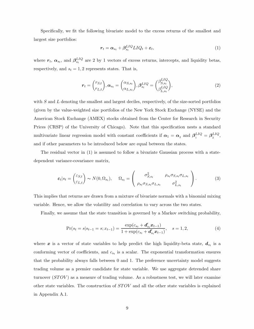
Specifically, we fit the following bivariate model to the excess returns of the smallest and

largest size portfolios:

rt = αst + βLIQst

LIQt + εt, (1)

where rt, αst, and βLIQst

are 2 by 1 vectors of excess returns, intercepts, and liquidity betas,

respectively, and st = 1, 2 represents states. That is,

rt =

(rS,t

rL,t

),αst =

(αS,st

αL,st

),βLIQ

st=

(βLIQ

S,st

βLIQL,st

), (2)

with S and L denoting the smallest and largest deciles, respectively, of the size-sorted portfolios

(given by the value-weighted size portfolios of the New York Stock Exchange (NYSE) and the

American Stock Exchange (AMEX) stocks obtained from the Center for Research in Security

Prices (CRSP) of the University of Chicago). Note that this specification nests a standard

multivariate linear regression model with constant coefficients if α1 = α2

and βLIQ1

= βLIQ2

,

and if other parameters to be introduced below are equal between the states.

The residual vector in (1) is assumed to follow a bivariate Gaussian process with a state-

dependent variance-covariance matrix,

εt|st =

(εS,t

εL,t

)∼ N(0,Ωst), Ωst =

σ2S,st

ρstσS,stσL,st

ρstσS,stσL,st σ2L,st

. (3)

This implies that returns are drawn from a mixture of bivariate normals with a binomial mixing

variable. Hence, we allow the volatility and correlation to vary across the two states.

Finally, we assume that the state transition is governed by a Markov switching probability,

Pr(st = s|st−1 = s;xt−1) =exp(cst + d′

stxt−1)

1 + exp(cst + d′st

xt−1), s = 1, 2, (4)

where x is a vector of state variables to help predict the high liquidity-beta state, dst is a

conforming vector of coefficients, and cst is a scalar. The exponential transformation ensures

that the probability always falls between 0 and 1. The preference uncertainty model suggests

trading volume as a premier candidate for state variable. We use aggregate detrended share

turnover (STOV ) as a measure of trading volume. As a robustness test, we will later examine

other state variables. The construction of STOV and all the other state variables is explained

in Appendix A.1.

9

Several comments about the above formulation follow. First, for ease of interpretation,

we have allowed only two possible states, st = 1 or 2, so that the parameters in equations

(1)-(4) are either (α1,βLIQ1 ,Ω1, c1,d1) if st = 1 or (α2,β

LIQ2 ,Ω2, c2,d2) if st = 2. Formally,

one could conduct a model specification test and search for the optimal number of states. The

resulting states, however, could be difficult to interpret. Our choice of two states allows us to

easily classify them as either a high or a low liquidity-beta state. This is also consistent with

the examples of Gallmeyer, Hollifield, and Seppi (2005) in which volume below a threshold

indicates no preference uncertainty and volume above it represents high preference uncertainty.

Second, the model imposes common states only for the smallest and largest deciles. Prefer-

ably, we wish to do so for a larger number of cross sections. This, however, makes the estimation

progressively more difficult because of the exploding number of parameters. For example, if

all the decile portfolios are used, the number of parameters to be estimated is 154 even with

two states and a single state variable. Our simple bivariate model with only one state variable

already has 18 parameters.3 In a later section, we will provide suggestive evidence to support

the use of the two extreme deciles; namely, liquidity betas vary almost monotonically across

ten liquidity-sorted portfolios in each of the two identified states.

Third, equation (1) does not control for factors typically used in asset pricing tests, especially

the market return. Aside from being parsimonious, this is appropriate and preferred for the

purpose of state identification. For example, if we included the market return, the estimated

liquidity betas would in one sense be those conditional on it. Rather, we know from existing

studies that unexpected liquidity shocks and the market return are correlated [see, e.g., Amihud

(2002)], and we consider the level of the market return to be an important characteristic of the

high liquidity-beta state.4 Needless to say, however, we will rigorously control for known factors

in our asset pricing tests.

Finally, we use excess returns on the CRSP size-sorted portfolios as dependent variables. An

obvious alternative is to use liquidity-sorted portfolios. We will show later that our results are

robust to such a change. Here, we emphasize the advantages of our choice. First, size portfolios

are known to produce significant cross-sectional variations in quantities of interest, such as

return, volatility, volume, and most importantly for our purpose, liquidity. Second, using the

3In general, an n variate version of our regime-switching model with two states and a single state variableinvolves n2 + 5n + 4 parameters.

4Nevertheless, we did estimate the system including the market return in equation (1). The basic asset pricingresults were not altered.

10

standard dataset facilitates the comparison of our results to the existing literature and suggests

directions for our robustness tests. For example, the CRSP size-sorted portfolios are also used

in the study of Amihud (2002). As he points out, we will later find that small firms’ returns are

more strongly affected by liquidity shocks than large firms’ returns. In addition to this cross-

sectional asymmetry, Perez-Quiros and Timmermann (2000) identify different dynamic patterns

in size-sorted portfolio returns; specifically, they find that small and large firms’ returns vary

asymmetrically over time across economic expansions and recessions due to their differential

exposures to credit risk. These findings clearly suggest the need to control for the size and

default risk factors in our asset pricing tests.

1.3 Data and Construction of the Liquidity Measure

We now describe the data and the construction of the liquidity measure. Researchers have

proposed several methods to create monthly liquidity series from standard datasets such as

CRSP over periods long enough for asset pricing tests. To be consistent with the notion of

illiquidity studied in Gallmeyer, Hollifield, and Seppi (2005), we choose Amihud’s (2002) price

impact proxy as a measure of illiquidity. It is simple to construct and yet is known to be highly

correlated with price impact measures calculated from high frequency data [Hasbrouck (2005)].

Following Amihud (2002), we first compute the price impact measure for individual stocks,

PRIM , as

PRIMj,t =1

Dj,t

Dj,t∑

d=1

|rj,d,t|

vj,d,t

, (5)

where rj,d,t and vj,d,t are the return and dollar volume (measured in millions), respectively, of

stock j on day d in month t, and Dj,t is the number of daily observations during that month.

We use ordinary common shares on NYSE and AMEX with Dj,t ≥ 15 and the beginning-of-

the-month price between $5 and $1, 000.5 The aggregate price impact, APRIM , is simply the

cross-sectional average of individual PRIM ,

APRIMt =1

Nt

Nt∑

j=1

PRIMj,t, (6)

where Nt is the number of stocks included in month t, which ranges between 1, 282 and 2, 129

5Following the common practice, NASDAQ stocks are excluded because their reported volumes may beoverstated due to the inclusion of inter-dealer trades.

11

from August 1962 through December 2004. Although the above formulation is based on an

equally weighted average, we obtain qualitatively similar asset pricing results when APRIM is

computed on a value weighted basis.6 Since APRIM is highly persistent, we fit the following

modified AR(2) model using the whole sample:7

(mt−1

m1APRIMt

)= α + β1

(mt−1

m1APRIMt−1

)+ β2

(mt−1

m1APRIMt−2

)+ εt, (7)

where mt−1 is the total market capitalization at month t − 1 of the stocks included in the

month t sample and m1 is the corresponding value for the initial month, August 1962. In the

above formulation, the ratio mt−1/m1 serves as a common detrending factor that controls for

the time trend in APRIM .8 Throughout the equation, the same factor is multiplied to the

contemporaneous and lagged APRIM to capture only the innovations in illiquidity; multiplying

lags of mt−1/m1 may introduce shocks induced mechanically by price changes. This adjustment

is used by Pastor and Stambaugh (2003) and Acharya and Pedersen (2005).

The errors in equation (7) are the measure of unexpected illiquidity shocks. We use the

negative estimated residuals, −εt, as our liquidity measure, LIQt. Panel (a) of Figure 1 plots

the time series of LIQ with dotted vertical lines representing the NBER business cycle dates

(each narrow band corresponds to a contraction). Occasional plunges in LIQ coincide with

major economic crises such as the Penn Central commercial paper debacle of May 1970, the

oil crisis of November 1973, the stock market crash (the Black Monday) of October 1987, the

Asian financial crisis of 1997, and the Russian bond default of 1998.

1.4 Empirical Estimation of the High Liquidity-Beta State

Table 1 reports the estimated parameters of the bivariate regime-switching model given in

equations (1)-(4) with STOV as the single state variable, x. The estimation is by maximum

likelihood using a monthly sample from January 1965 through December 2004.9

Consistent with Amihud (2002) and Acharya and Pedersen (2005), we observe significant

positive relationships between liquidity shocks and contemporaneous returns, as indicated by

6The results are available upon request.7APRIM has the first and second-order autocorrelations of 0.878 and 0.858, respectively, whereas the liquidity

shock, LIQ, to be introduced below, has a first-order autocorrelation of only -0.020.8APRIM has generally decreased over time with an exception from the late 1990’s through the early 2000’s

when market volatility increased substantially. The declining trend is due to a steady increase in trading volume.9We lose the first two years of STOV due to its detrending method described in Appendix A.1. To align the

sample period for all the variables, we use the period starting in January 1965.

12

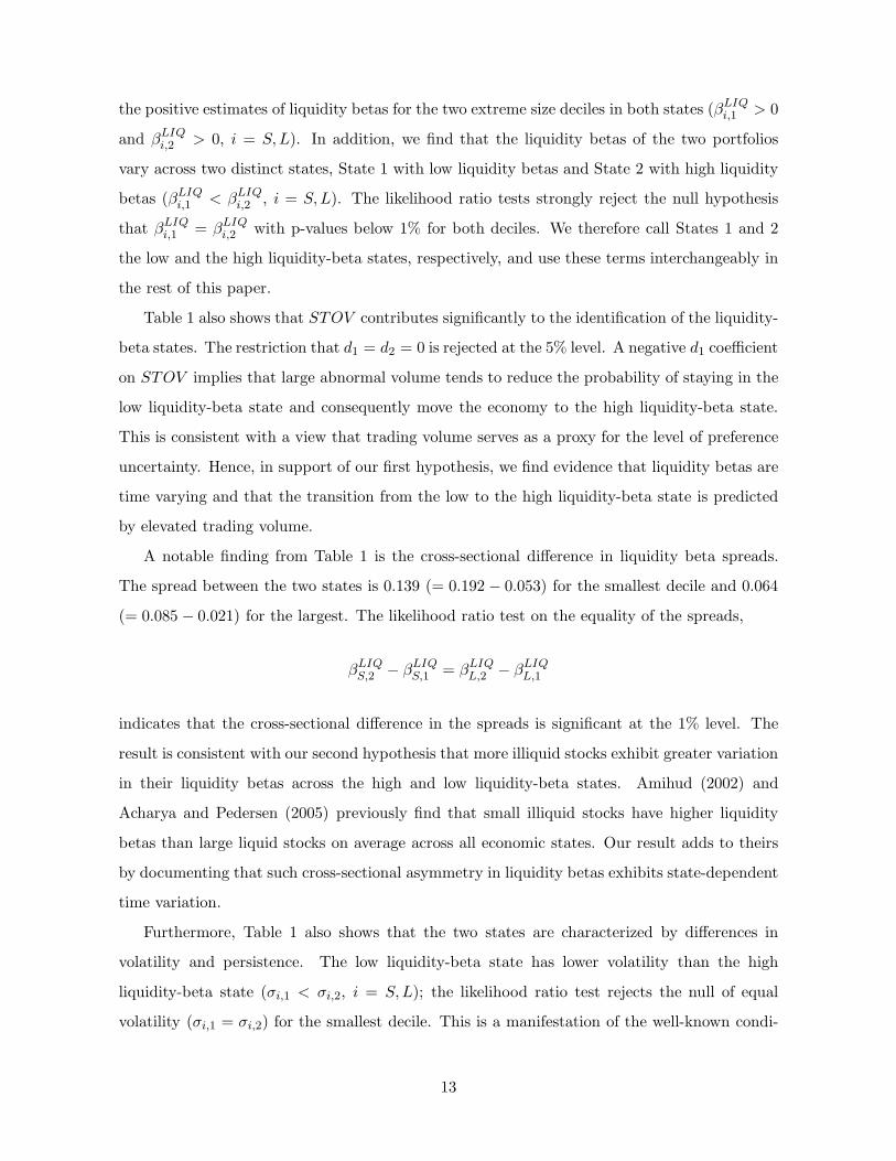
the positive estimates of liquidity betas for the two extreme size deciles in both states (βLIQi,1 > 0

and βLIQi,2 > 0, i = S,L). In addition, we find that the liquidity betas of the two portfolios

vary across two distinct states, State 1 with low liquidity betas and State 2 with high liquidity

betas (βLIQi,1 < βLIQ

i,2 , i = S,L). The likelihood ratio tests strongly reject the null hypothesis

that βLIQi,1 = βLIQ

i,2 with p-values below 1% for both deciles. We therefore call States 1 and 2

the low and the high liquidity-beta states, respectively, and use these terms interchangeably in

the rest of this paper.

Table 1 also shows that STOV contributes significantly to the identification of the liquidity-

beta states. The restriction that d1 = d2 = 0 is rejected at the 5% level. A negative d1 coefficient

on STOV implies that large abnormal volume tends to reduce the probability of staying in the

low liquidity-beta state and consequently move the economy to the high liquidity-beta state.

This is consistent with a view that trading volume serves as a proxy for the level of preference

uncertainty. Hence, in support of our first hypothesis, we find evidence that liquidity betas are

time varying and that the transition from the low to the high liquidity-beta state is predicted

by elevated trading volume.

A notable finding from Table 1 is the cross-sectional difference in liquidity beta spreads.

The spread between the two states is 0.139 (= 0.192 − 0.053) for the smallest decile and 0.064

(= 0.085 − 0.021) for the largest. The likelihood ratio test on the equality of the spreads,

βLIQS,2 − βLIQ

S,1 = βLIQL,2 − βLIQ

L,1

indicates that the cross-sectional difference in the spreads is significant at the 1% level. The

result is consistent with our second hypothesis that more illiquid stocks exhibit greater variation

in their liquidity betas across the high and low liquidity-beta states. Amihud (2002) and

Acharya and Pedersen (2005) previously find that small illiquid stocks have higher liquidity

betas than large liquid stocks on average across all economic states. Our result adds to theirs

by documenting that such cross-sectional asymmetry in liquidity betas exhibits state-dependent

time variation.

Furthermore, Table 1 also shows that the two states are characterized by differences in

volatility and persistence. The low liquidity-beta state has lower volatility than the high

liquidity-beta state (σi,1 < σi,2, i = S,L); the likelihood ratio test rejects the null of equal

volatility (σi,1 = σi,2) for the smallest decile. This is a manifestation of the well-known condi-

13

tional heteroskedasticity in stock returns. Moreover, the high liquidity-beta state is less persis-

tent than the low liquidity-beta state. The average durations of the low and high liquidity-beta

states evaluated at mean STOV are 8.3 and 1.7 months, respectively.10 This point is graphi-

cally demonstrated in Panel (b) of Figure 1, which plots the estimated probability of being in

the high liquidity-beta state. It is visually clear that whenever the probability rises up close

to 1, it drops back quickly within a few months. The short duration of the high liquidity-beta

state is consistent with the feature of an ‘abnormal’ state. The sharp spikes in the probability

coincide with some of the economic crises noted earlier, such as the Black Monday of October

1987 and the Russian bond default of August 1998. However, they also include non-crisis pe-

riods, and in fact many of them do not correspond to the LIQ plunges in Panel (a). We will

later observe that the high liquidity-beta state is a mixture of months with large positive and

negative liquidity shocks accompanied by elevated trading volume.

Overall, consistent with the preference uncertainty story, our analysis shows that liquidity

betas are high and exhibit a large cross-sectional dispersion during periods of high trading

volume.

1.5 Alternative State Variables

Before conducting asset pricing tests, this section examines whether different state variables

can also predict the high liquidity-beta state. The first alternative we consider is the aggregate

volatility (V OL). In the preference uncertainty model, volatility is expected to rise in the

state of high preference uncertainty where trading reveals more information about investors’

future asset demands [Gallmeyer, Hollifield, and Seppi (2005)]. Elevated volatility can thus be

an indirect sign of heightened preference risk and increased probability of the high liquidity-

beta state occurring. In a different context, Vayanos (2004) also emphasizes the role of market

volatility in the variation of illiquidity premium. In his model, investors are assumed to be fund

managers subject to fund withdrawals when their performance falls below a threshold. Since

their fee income is proportional to the size of the funds they manage, their preference toward

liquid assets rises during volatile times. This creates time variation in risk premium induced by

changing volatility. In contrast to the preference uncertainty model, however, there is no role

10The mean of STOV is x = 0.1472 and 0.1979 for States 1 and 2, respectively (see Panel (b) of Table 5).Using the parameter estimates from Table 1, cs +dsx is 1.992 ≡ f1 for State 1 and −0.293 ≡ f2 for State 2. Thisgives ef1/(1 + ef1) = 0.880 ≡ p and ef2/(1 + ef2) = 0.427 ≡ q. The average durations in the text are given by1/(1 − p) and 1/(1 − q).

14

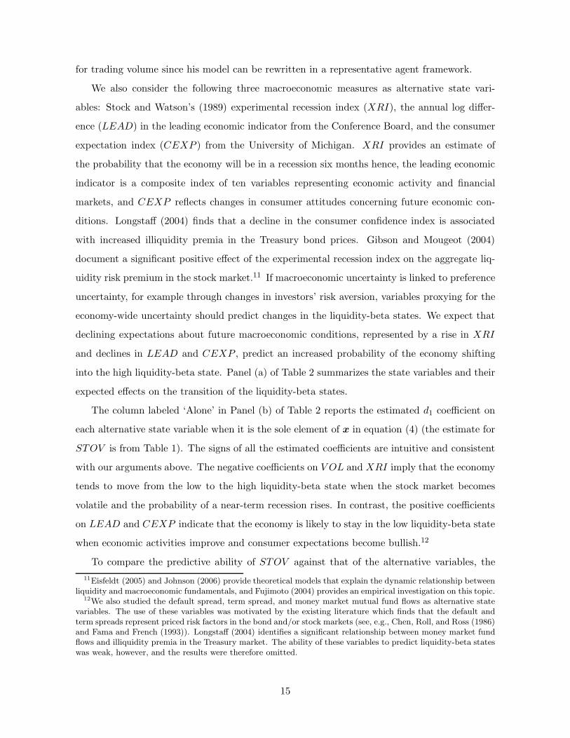
for trading volume since his model can be rewritten in a representative agent framework.

We also consider the following three macroeconomic measures as alternative state vari-

ables: Stock and Watson’s (1989) experimental recession index (XRI), the annual log differ-

ence (LEAD) in the leading economic indicator from the Conference Board, and the consumer

expectation index (CEXP ) from the University of Michigan. XRI provides an estimate of

the probability that the economy will be in a recession six months hence, the leading economic

indicator is a composite index of ten variables representing economic activity and financial

markets, and CEXP reflects changes in consumer attitudes concerning future economic con-

ditions. Longstaff (2004) finds that a decline in the consumer confidence index is associated

with increased illiquidity premia in the Treasury bond prices. Gibson and Mougeot (2004)

document a significant positive effect of the experimental recession index on the aggregate liq-

uidity risk premium in the stock market.11 If macroeconomic uncertainty is linked to preference

uncertainty, for example through changes in investors’ risk aversion, variables proxying for the

economy-wide uncertainty should predict changes in the liquidity-beta states. We expect that

declining expectations about future macroeconomic conditions, represented by a rise in XRI

and declines in LEAD and CEXP , predict an increased probability of the economy shifting

into the high liquidity-beta state. Panel (a) of Table 2 summarizes the state variables and their

expected effects on the transition of the liquidity-beta states.

The column labeled ‘Alone’ in Panel (b) of Table 2 reports the estimated d1 coefficient on

each alternative state variable when it is the sole element of x in equation (4) (the estimate for

STOV is from Table 1). The signs of all the estimated coefficients are intuitive and consistent

with our arguments above. The negative coefficients on V OL and XRI imply that the economy

tends to move from the low to the high liquidity-beta state when the stock market becomes

volatile and the probability of a near-term recession rises. In contrast, the positive coefficients

on LEAD and CEXP indicate that the economy is likely to stay in the low liquidity-beta state

when economic activities improve and consumer expectations become bullish.12

To compare the predictive ability of STOV against that of the alternative variables, the

11Eisfeldt (2005) and Johnson (2006) provide theoretical models that explain the dynamic relationship betweenliquidity and macroeconomic fundamentals, and Fujimoto (2004) provides an empirical investigation on this topic.

12We also studied the default spread, term spread, and money market mutual fund flows as alternative statevariables. The use of these variables was motivated by the existing literature which finds that the default andterm spreads represent priced risk factors in the bond and/or stock markets (see, e.g., Chen, Roll, and Ross (1986)and Fama and French (1993)). Longstaff (2004) identifies a significant relationship between money market fundflows and illiquidity premia in the Treasury market. The ability of these variables to predict liquidity-beta stateswas weak, however, and the results were therefore omitted.

15

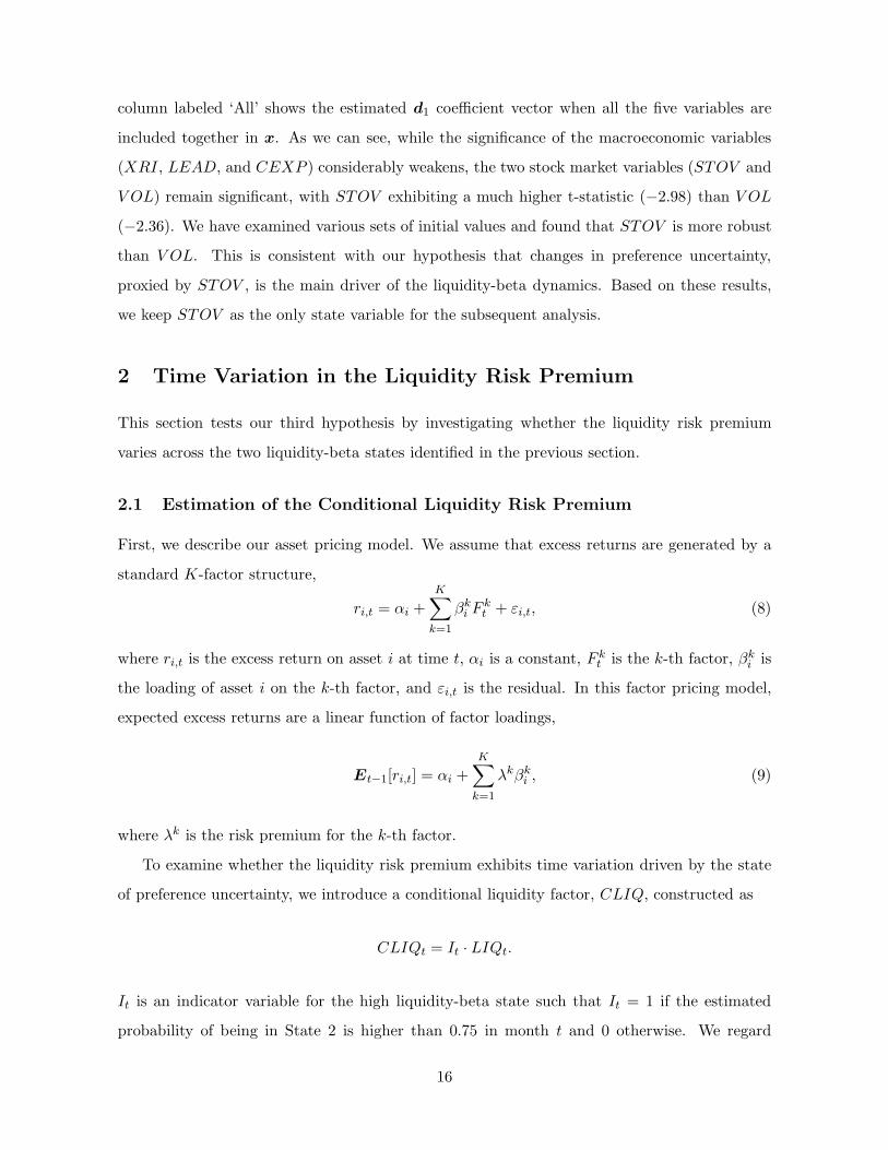
column labeled ‘All’ shows the estimated d1 coefficient vector when all the five variables are

included together in x. As we can see, while the significance of the macroeconomic variables

(XRI, LEAD, and CEXP ) considerably weakens, the two stock market variables (STOV and

V OL) remain significant, with STOV exhibiting a much higher t-statistic (−2.98) than V OL

(−2.36). We have examined various sets of initial values and found that STOV is more robust

than V OL. This is consistent with our hypothesis that changes in preference uncertainty,

proxied by STOV , is the main driver of the liquidity-beta dynamics. Based on these results,

we keep STOV as the only state variable for the subsequent analysis.

2 Time Variation in the Liquidity Risk Premium

This section tests our third hypothesis by investigating whether the liquidity risk premium

varies across the two liquidity-beta states identified in the previous section.

2.1 Estimation of the Conditional Liquidity Risk Premium

First, we describe our asset pricing model. We assume that excess returns are generated by a

standard K-factor structure,

ri,t = αi +

K∑

k=1

βki F k

t + εi,t, (8)

where ri,t is the excess return on asset i at time t, αi is a constant, F kt is the k-th factor, βk

i is

the loading of asset i on the k-th factor, and εi,t is the residual. In this factor pricing model,

expected excess returns are a linear function of factor loadings,

Et−1[ri,t] = αi +K∑

k=1

λkβki , (9)

where λk is the risk premium for the k-th factor.

To examine whether the liquidity risk premium exhibits time variation driven by the state

of preference uncertainty, we introduce a conditional liquidity factor, CLIQ, constructed as

CLIQt = It · LIQt.

It is an indicator variable for the high liquidity-beta state such that It = 1 if the estimated

probability of being in State 2 is higher than 0.75 in month t and 0 otherwise. We regard

16

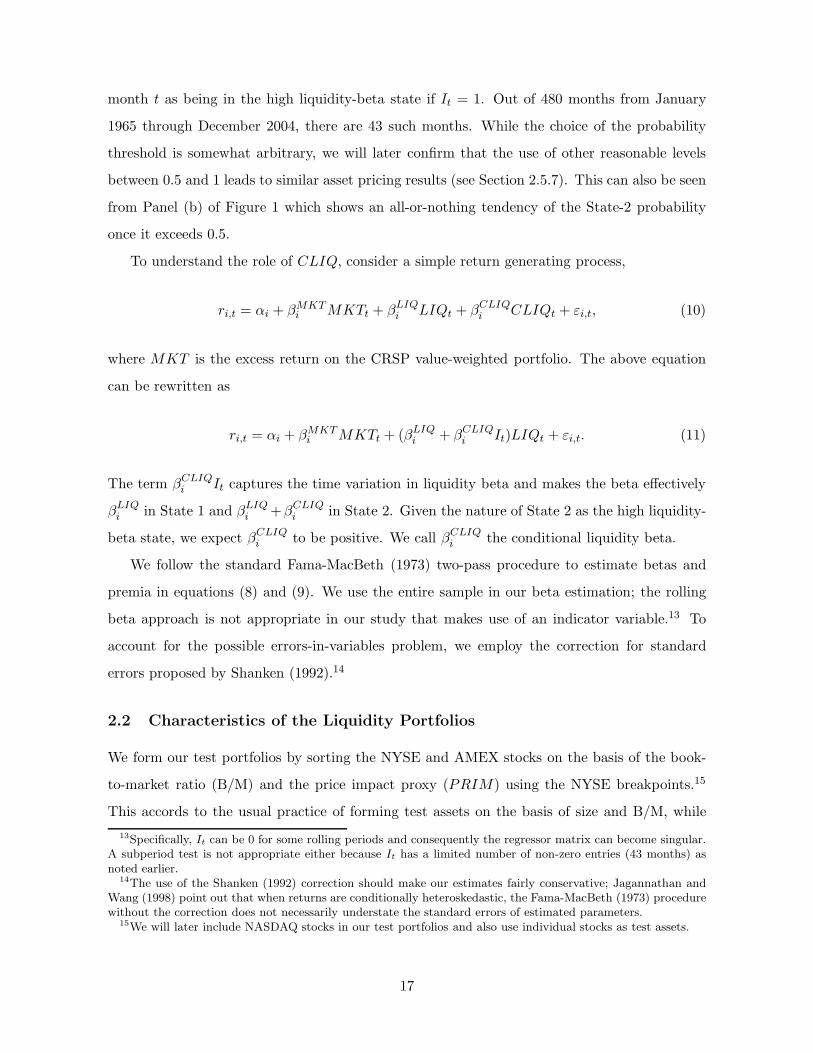
month t as being in the high liquidity-beta state if It = 1. Out of 480 months from January

1965 through December 2004, there are 43 such months. While the choice of the probability

threshold is somewhat arbitrary, we will later confirm that the use of other reasonable levels

between 0.5 and 1 leads to similar asset pricing results (see Section 2.5.7). This can also be seen

from Panel (b) of Figure 1 which shows an all-or-nothing tendency of the State-2 probability

once it exceeds 0.5.

To understand the role of CLIQ, consider a simple return generating process,

ri,t = αi + βMKTi MKTt + βLIQ

i LIQt + βCLIQi CLIQt + εi,t, (10)

where MKT is the excess return on the CRSP value-weighted portfolio. The above equation

can be rewritten as

ri,t = αi + βMKTi MKTt + (βLIQ

i + βCLIQi It)LIQt + εi,t. (11)

The term βCLIQi It captures the time variation in liquidity beta and makes the beta effectively

βLIQi in State 1 and βLIQ

i +βCLIQi in State 2. Given the nature of State 2 as the high liquidity-

beta state, we expect βCLIQi to be positive. We call βCLIQ

i the conditional liquidity beta.

We follow the standard Fama-MacBeth (1973) two-pass procedure to estimate betas and

premia in equations (8) and (9). We use the entire sample in our beta estimation; the rolling

beta approach is not appropriate in our study that makes use of an indicator variable.13 To

account for the possible errors-in-variables problem, we employ the correction for standard

errors proposed by Shanken (1992).14

2.2 Characteristics of the Liquidity Portfolios

We form our test portfolios by sorting the NYSE and AMEX stocks on the basis of the book-

to-market ratio (B/M) and the price impact proxy (PRIM) using the NYSE breakpoints.15

This accords to the usual practice of forming test assets on the basis of size and B/M, while

13Specifically, It can be 0 for some rolling periods and consequently the regressor matrix can become singular.A subperiod test is not appropriate either because It has a limited number of non-zero entries (43 months) asnoted earlier.

14The use of the Shanken (1992) correction should make our estimates fairly conservative; Jagannathan andWang (1998) point out that when returns are conditionally heteroskedastic, the Fama-MacBeth (1973) procedurewithout the correction does not necessarily understate the standard errors of estimated parameters.

15We will later include NASDAQ stocks in our test portfolios and also use individual stocks as test assets.

17

recognizing the fact that the size and liquidity characteristics are cross-sectionally highly corre-

lated. Balancing the desire to produce sufficient dispersion in liquidity betas and to represent as

diverse cross sections as possible, we replace size with PRIM . Later, however, we will explicitly

include size in the sorting keys to make sure this does not unduly favor our result. The portfo-

lios are formed at the end of each year from 1964 through 2003, and the value-weighted monthly

portfolio returns are calculated for the subsequent years from January 1965 through December

2004. Stocks are admitted to portfolios if they have the end-of-the-year prices between $5 and

$1000 and more than 100 daily-return observations during the year.

We first look at the characteristics of the decile portfolios sorted only on PRIM as summa-

rized in Panel (a) of Table 3. Rank 1 represents the lowest PRIM (most liquid) and rank 10 the

highest (least liquid). Appendix A.2 describes the computation of characteristics. Consistent

with our prior knowledge about illiquidity premium, the average raw return, r, generally in-

creases with PRIM and so does a return volatility measure, σr. A monotonic increase in PRIM

and the absolute value of Pastor and Stambaugh’s (2003) return reversal measure (RREV ) in-

dicates that we continue to get dispersion in illiquidity levels after portfolio formation. All the

other characteristics exhibit expected near-monotonic relations with the PRIM ranking; more

illiquid stocks tend to have more volatile PRIM (σPRIM ), lower turnover ratio (TOV ), lower

price (PRC), smaller market capitalization, and greater B/M ratio (although the relation for

TOV is not strictly monotone). These results suggest that it is important to control for the

size and value factors as well as the illiquidity characteristic in our asset pricing tests. The

disproportionately large average number of stocks (N) in the most illiquid portfolio indicates

that AMEX stocks are much less liquid than NYSE stocks in general.

The last two columns show the estimated portfolio betas on LIQ and CLIQ in equation

(10). We observe that both βLIQ and βCLIQ increase almost monotonically with PRIM . The

two betas are negative for the most liquid portfolio because they are estimated conditional

on MKT in the multiple regression; the adjustment for MKT reduces the liquidity effect

on portfolio returns since MKT and LIQ are positively correlated. Hence, the result that

βCLIQ < βLIQ for liquid portfolios is due to this conditioning and does not invalidate State 2

as being the high liquidity-beta state. Importantly, the cross-sectional dispersion in βCLIQ is

much larger than the dispersion in βLIQ; the difference between the two extreme PRIM deciles

is 0.067 for βCLIQ as opposed to 0.034 for βLIQ. Figure 2 demonstrates this point graphically.

Since βCLIQ is the beta spread between the two states (see equation (11)), the dispersion in

18

State-2 liquidity betas between the extreme deciles is the sum of these two numbers, 0.101.

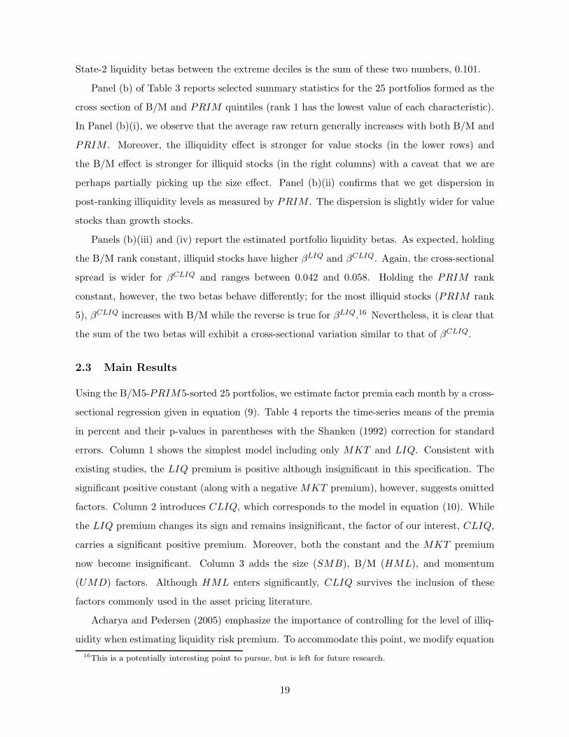
Panel (b) of Table 3 reports selected summary statistics for the 25 portfolios formed as the

cross section of B/M and PRIM quintiles (rank 1 has the lowest value of each characteristic).

In Panel (b)(i), we observe that the average raw return generally increases with both B/M and

PRIM . Moreover, the illiquidity effect is stronger for value stocks (in the lower rows) and

the B/M effect is stronger for illiquid stocks (in the right columns) with a caveat that we are

perhaps partially picking up the size effect. Panel (b)(ii) confirms that we get dispersion in

post-ranking illiquidity levels as measured by PRIM . The dispersion is slightly wider for value

stocks than growth stocks.

Panels (b)(iii) and (iv) report the estimated portfolio liquidity betas. As expected, holding

the B/M rank constant, illiquid stocks have higher βLIQ and βCLIQ. Again, the cross-sectional

spread is wider for βCLIQ and ranges between 0.042 and 0.058. Holding the PRIM rank

constant, however, the two betas behave differently; for the most illiquid stocks (PRIM rank

5), βCLIQ increases with B/M while the reverse is true for βLIQ.16 Nevertheless, it is clear that

the sum of the two betas will exhibit a cross-sectional variation similar to that of βCLIQ.

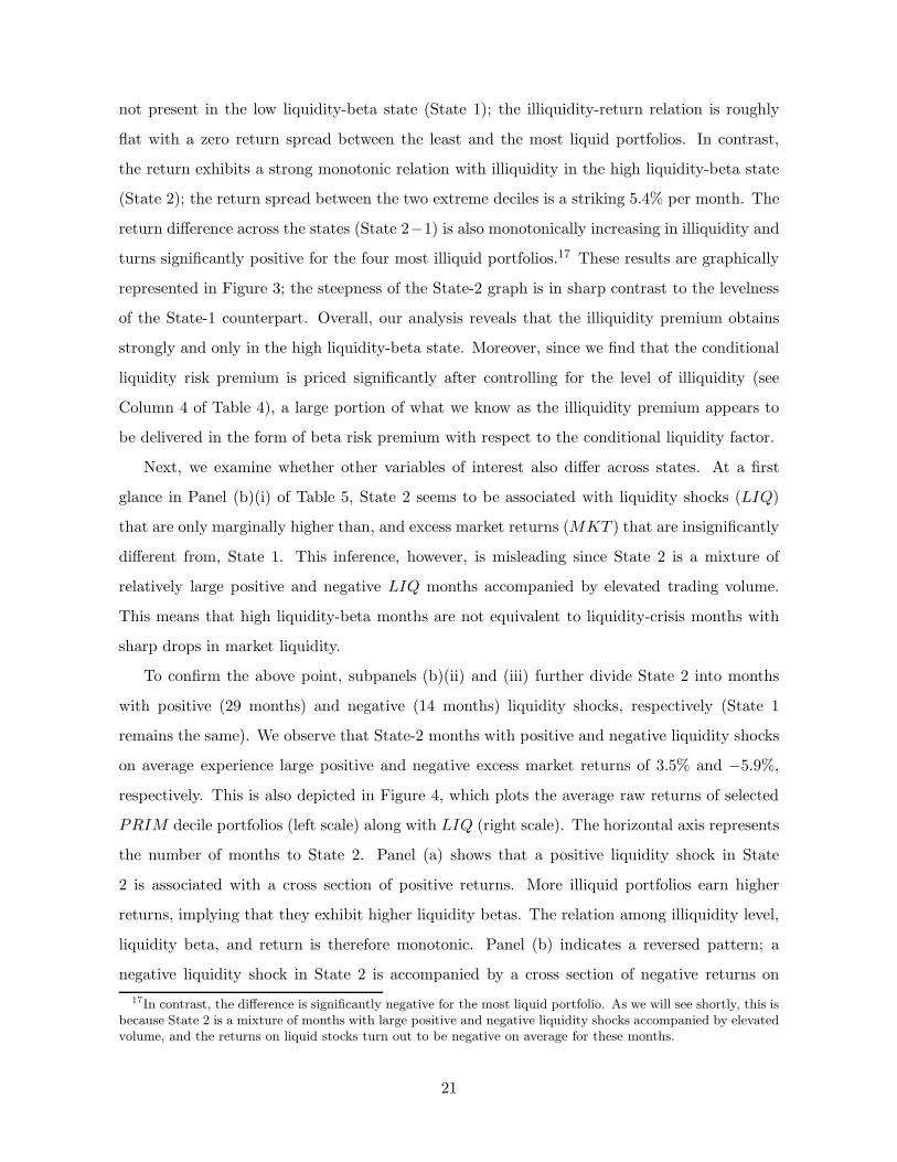
2.3 Main Results

Using the B/M5-PRIM5-sorted 25 portfolios, we estimate factor premia each month by a cross-

sectional regression given in equation (9). Table 4 reports the time-series means of the premia

in percent and their p-values in parentheses with the Shanken (1992) correction for standard

errors. Column 1 shows the simplest model including only MKT and LIQ. Consistent with

existing studies, the LIQ premium is positive although insignificant in this specification. The

significant positive constant (along with a negative MKT premium), however, suggests omitted

factors. Column 2 introduces CLIQ, which corresponds to the model in equation (10). While

the LIQ premium changes its sign and remains insignificant, the factor of our interest, CLIQ,

carries a significant positive premium. Moreover, both the constant and the MKT premium

now become insignificant. Column 3 adds the size (SMB), B/M (HML), and momentum

(UMD) factors. Although HML enters significantly, CLIQ survives the inclusion of these

factors commonly used in the asset pricing literature.

Acharya and Pedersen (2005) emphasize the importance of controlling for the level of illiq-

uidity when estimating liquidity risk premium. To accommodate this point, we modify equation

16This is a potentially interesting point to pursue, but is left for future research.

19

(9) to include characteristics of the test portfolios [Daniel and Titman (1997)]:

Et−1[ri,t] = αi +K∑

k=1

λkβki +

M∑

m=1

λmθmi,t−1, (12)

where θmi,t−1 is the m-th characteristic for portfolio i at the end of month t−1. Using the lagged

portfolio PRIM as the only characteristic in equation (12), Column 4 of Table 4 indicates that

the CLIQ premium is robust to the inclusion of the illiquidity characteristic and is estimated to

be 10.2% per unit beta. Note that CLIQ is a non-traded factor and therefore its premium is not

directly comparable to others’. We will later examine the economic significance of the CLIQ

premium using a factor mimicking portfolio. We will also control for other firm characteristics

in the robustness test section.

The significant positive premium on CLIQ supports our third hypothesis that the liquidity

risk premium is time varying and is greater during periods of high preference uncertainty.

Combined with our results from the previous sections, we find that both high liquidity betas

and large liquidity risk premium arise simultaneously during periods of high trading volume.

2.4 Characteristics of the High Liquidity-Beta State

Given the evidence on the conditional pricing of liquidity risk in the cross section of stock

returns, this section examines the characteristics of the high liquidity-beta state in more detail.

2.4.1 Illiquidity Premium and Liquidity Risk Premium

First, we study the state-dependent relationship between illiquidity premium and liquidity risk

premium. In the preference uncertainty story, the periods of heightened preference risk with

high premium are accompanied by greater stock price sensitivities to order flow because trad-

ing is more informative about future asset demands during these times. The level of illiquidity,

measured by the price impact of trade, therefore appears to be priced in the state of high pref-

erence uncertainty [Gallmeyer, Hollifield, and Seppi (2005)]. Given the link between preference

uncertainty and illiquidity premium, we expect that the periods of high liquidity betas and high

liquidity risk premium also represent times of high illiquidity premium.

Panel (a) of Table 5 reports average monthly excess returns of the PRIM -sorted decile

portfolios by state. Consistent with the usual notion of illiquidity premium, the unconditional

return increases with the level of illiquidity (column labeled ‘All’). This pattern, however, is

20

not present in the low liquidity-beta state (State 1); the illiquidity-return relation is roughly

flat with a zero return spread between the least and the most liquid portfolios. In contrast,

the return exhibits a strong monotonic relation with illiquidity in the high liquidity-beta state

(State 2); the return spread between the two extreme deciles is a striking 5.4% per month. The

return difference across the states (State 2−1) is also monotonically increasing in illiquidity and

turns significantly positive for the four most illiquid portfolios.17 These results are graphically

represented in Figure 3; the steepness of the State-2 graph is in sharp contrast to the levelness

of the State-1 counterpart. Overall, our analysis reveals that the illiquidity premium obtains

strongly and only in the high liquidity-beta state. Moreover, since we find that the conditional

liquidity risk premium is priced significantly after controlling for the level of illiquidity (see

Column 4 of Table 4), a large portion of what we know as the illiquidity premium appears to

be delivered in the form of beta risk premium with respect to the conditional liquidity factor.

Next, we examine whether other variables of interest also differ across states. At a first

glance in Panel (b)(i) of Table 5, State 2 seems to be associated with liquidity shocks (LIQ)

that are only marginally higher than, and excess market returns (MKT ) that are insignificantly

different from, State 1. This inference, however, is misleading since State 2 is a mixture of

relatively large positive and negative LIQ months accompanied by elevated trading volume.

This means that high liquidity-beta months are not equivalent to liquidity-crisis months with

sharp drops in market liquidity.

To confirm the above point, subpanels (b)(ii) and (iii) further divide State 2 into months

with positive (29 months) and negative (14 months) liquidity shocks, respectively (State 1

remains the same). We observe that State-2 months with positive and negative liquidity shocks

on average experience large positive and negative excess market returns of 3.5% and −5.9%,

respectively. This is also depicted in Figure 4, which plots the average raw returns of selected

PRIM decile portfolios (left scale) along with LIQ (right scale). The horizontal axis represents

the number of months to State 2. Panel (a) shows that a positive liquidity shock in State

2 is associated with a cross section of positive returns. More illiquid portfolios earn higher

returns, implying that they exhibit higher liquidity betas. The relation among illiquidity level,

liquidity beta, and return is therefore monotonic. Panel (b) indicates a reversed pattern; a

negative liquidity shock in State 2 is accompanied by a cross section of negative returns on

17In contrast, the difference is significantly negative for the most liquid portfolio. As we will see shortly, this isbecause State 2 is a mixture of months with large positive and negative liquidity shocks accompanied by elevatedvolume, and the returns on liquid stocks turn out to be negative on average for these months.

21

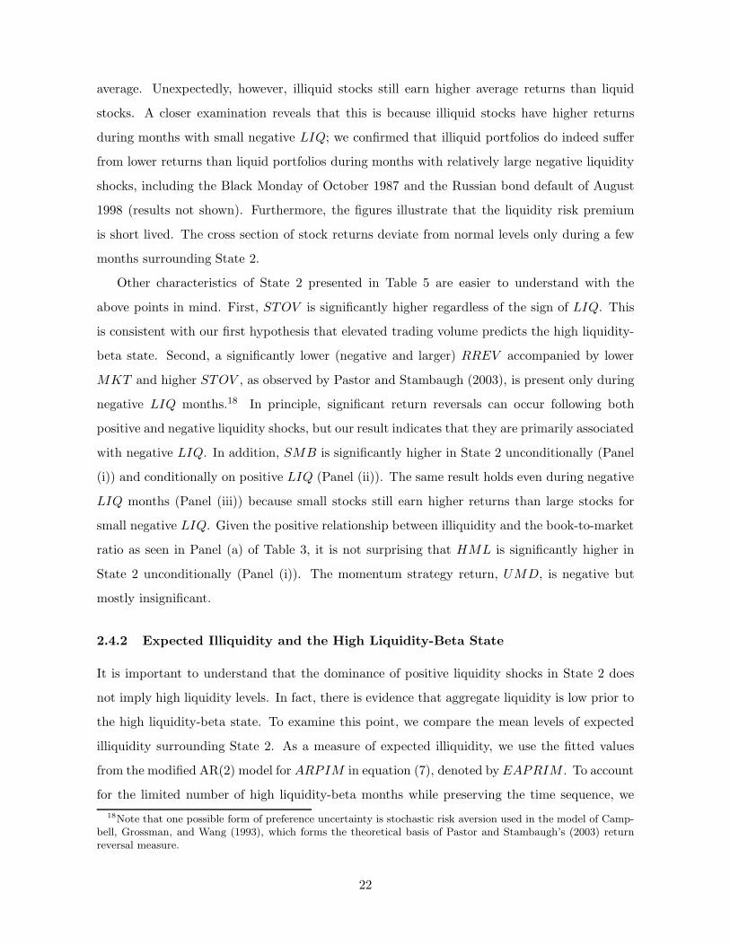
average. Unexpectedly, however, illiquid stocks still earn higher average returns than liquid

stocks. A closer examination reveals that this is because illiquid stocks have higher returns

during months with small negative LIQ; we confirmed that illiquid portfolios do indeed suffer

from lower returns than liquid portfolios during months with relatively large negative liquidity

shocks, including the Black Monday of October 1987 and the Russian bond default of August

1998 (results not shown). Furthermore, the figures illustrate that the liquidity risk premium

is short lived. The cross section of stock returns deviate from normal levels only during a few

months surrounding State 2.

Other characteristics of State 2 presented in Table 5 are easier to understand with the

above points in mind. First, STOV is significantly higher regardless of the sign of LIQ. This

is consistent with our first hypothesis that elevated trading volume predicts the high liquidity-

beta state. Second, a significantly lower (negative and larger) RREV accompanied by lower

MKT and higher STOV , as observed by Pastor and Stambaugh (2003), is present only during

negative LIQ months.18 In principle, significant return reversals can occur following both

positive and negative liquidity shocks, but our result indicates that they are primarily associated

with negative LIQ. In addition, SMB is significantly higher in State 2 unconditionally (Panel

(i)) and conditionally on positive LIQ (Panel (ii)). The same result holds even during negative

LIQ months (Panel (iii)) because small stocks still earn higher returns than large stocks for

small negative LIQ. Given the positive relationship between illiquidity and the book-to-market

ratio as seen in Panel (a) of Table 3, it is not surprising that HML is significantly higher in

State 2 unconditionally (Panel (i)). The momentum strategy return, UMD, is negative but

mostly insignificant.

2.4.2 Expected Illiquidity and the High Liquidity-Beta State

It is important to understand that the dominance of positive liquidity shocks in State 2 does

not imply high liquidity levels. In fact, there is evidence that aggregate liquidity is low prior to

the high liquidity-beta state. To examine this point, we compare the mean levels of expected

illiquidity surrounding State 2. As a measure of expected illiquidity, we use the fitted values

from the modified AR(2) model for ARPIM in equation (7), denoted by EAPRIM . To account

for the limited number of high liquidity-beta months while preserving the time sequence, we

18Note that one possible form of preference uncertainty is stochastic risk aversion used in the model of Camp-bell, Grossman, and Wang (1993), which forms the theoretical basis of Pastor and Stambaugh’s (2003) returnreversal measure.

22

conduct block bootstraps. Specifically, each sampling draws 43 blocks of fitted EAPRIM with

replacement. Each block starts at nine months prior to a high liquidity-beta state and continues

through nine months after it. Within each block, we compute the difference between EAPRIM

and its block average monthly. The differences are then averaged across the 43 drawn blocks

month-by-month. This is repeated 5000 times, and the means and the 95% confidence intervals

of the monthly differences across the re-samplings are calculated. Panel (a) of Figure 5 shows

the bootstrap means with a solid line and the confidence intervals with dashed lines. To get

a sense of the level, the mean of the block averages is added back and is shown by a dotted

horizontal line. We observe that EAPRIM rises significantly above the block mean several

months prior to the high liquidity-beta state, then falls significantly below the mean a couple

of months afterward before finally reverting back toward the average level.

We can see a similar dynamics for another measure of expected illiquidity in Panel (b),

which simply plots the lagged APRIM (denoted by LAPRIM) without trend adjustment.19

LAPRIM is also used as a measure of expected illiquidity in Amihud (2002). Further, to ex-

amine the pervasiveness of this illiquidity variation around State 2, Panels (c) and (d) conduct

the same bootstrapping analysis for the lagged PRIM characteristics of the most (LPRIM01)

and the least (LPRIM10) liquid PRIM -sorted deciles, respectively. Lagged PRIM charac-

teristics of other deciles exhibit similar dynamics and fall somewhere between these two series

(results not shown). From these figures, it appears reasonable to consider that investors expect

deteriorating future liquidity several months prior to the high liquidity-beta state, leading to

a rise in illiquidity premium. This again confirms that the times of high illiquidity premium

roughly coincide with times of high liquidity risk premium.

Panels (e)-(i) of Figure 5 depict the bootstrap means of the five state variables studied

in Section 1.5. Consistent with our first hypothesis, Panel (e) indicates highly elevated share

turnover around the high liquidity-beta state. This is also accompanied by a significant rise in

volatility (Panel (f)) although the increase is more substantial for STOV . In addition, several

months before the high liquidity-beta state, XRI and LEAD significantly deviate from the

mean in the direction consistent with the traditional risk story; the probability of entering

into a near-term recession rises (Panel (g)) and the leading indicator of economic conditions

declines (Panel (h)). Past the high liquidity-beta month, the two measures cross the means and

19Possible nonstationarity of unadjusted APRIM is not an issue here since the average is taken within eachblock.

23

deviate away from them in the opposite direction. Finally, Panel (i) shows that the deviation

of CEXP from the block average is not significant but also goes in the right direction.20

These results are consistent with the findings of Longstaff (2004) and Gibson and Mougeot

(2004). Overall, while the pricing of liquidity risk can and does occur at a frequency different

from that of business cycles, there is some association between the liquidity risk premium and

macroeconomic conditions.

2.5 Robustness Tests

This section conducts a number of robustness tests on the conditional pricing of liquidity risk.

We first control for additional factors and characteristics that are likely to be correlated with

liquidity risk. We then examine if our pricing results hold for different test assets and alternative

methods of state identification. The effect of outliers is also discussed.

2.5.1 Size and B/M Characteristics

Daniel and Titman (1997) argue that the size and B/M premia arise because of such character-

istics per se rather than beta risks with respect to these factors. To control for this possibility,

we replace SMB and HML in Columns 3 and 4 of Table 4 with the lagged size and B/M

characteristics of the test portfolios as in equation (12). The results are presented in Table 6.

While lowered to about 8% in the presence of strong size effect, the CLIQ premium is still

significant at the 5% level with or without the level of illiquidity.

2.5.2 Conditional Size and B/M Factors

Recall from Panel (b) of Table 5 that SMB and HML have higher returns in the high liquidity-

beta state. This raises a concern as to whether the observed conditional liquidity effect is

a conditional size or book-to-market effect in disguise. In fact, Guidolin and Timmermann

(2005) find that size and value premia vary across economic regimes, and Perez-Quiros and

Timmermann (2000) report that the small-firm premium increases sharply during late stages

20We also plotted variables in Panels (a)-(i) conditional on the sign of LIQ in State 2. Generally, the dynamicsaround State 2 with positive LIQ are similar or reinforced for all the variables except for V OL, which exhibitsno variation.

24

of most recessions. To address this concern, we construct conditional size and value factors as

CSMBt = It · SMBt,

CHMLt = It · HMLt,

where It is again the indicator variable that defines the high liquidity-beta state. Table 7 shows

the estimated premia. The magnitude of the CLIQ premium is almost unchanged at around

9% to 10% at the 5% significance level upon the inclusion of CSMB, CHML, or both. The

effects of CSMB and CHML are insignificant, suggesting that the liquidity-beta states we

identified are distinct from economic regimes underlying the variations of the size and value

premia.

2.5.3 Default and Aggregate Volatility Factors

It is sensible to suspect that liquidity risk is correlated with default risk because illiquid firms

tend to be small firms that are relatively likely to default. Perez-Quiros and Timmermann

(2000) find evidence of asymmetry in the small and large firms’ exposures to credit risk across

recession and expansion states. To control for the possible effect of default risk, we include

Vassalou and Xing’s (2004) default factor (DSV ) in our test.21

We also recall that our regime-switching model allowed volatility to vary across states. While

we consider volatility an important characteristic of the high liquidity-beta state, it may also

introduce a pseudo pricing effect; researchers have shown that stocks with higher sensitivity to

innovations in aggregate volatility tend to earn lower returns [Ang, Hodrick, Xing, and Zhang

(2006)]. To account for this, we additionally include an aggregate volatility factor (dV OL)

given by the monthly first-order differences in V OL.22

The results are given in Column 1 of Table 8, which shows that the CLIQ premium is robust

to the inclusion of DSV and dV OL. Note that the availability of DSV restricts the sample

period to January 1971 through December 1999 (N = 348). In this shorter sample period, the

illiquidity characteristic, PRIM , is significantly priced. In a separate test, we also examined

21We thank Maria Vassalou for making the default factor available on her web site.22Ang, Hodrick, Xing, and Zhang (2006) construct a monthly mimicking portfolio of the innovations in ag-

gregate volatility, where the innovations are given by the daily difference of the V IX index from the ChicagoBoard Options Exchange (CBOE). Instead of constructing a factor mimicking portfolio, we directly use changesin aggregate volatility as a non-traded factor. We do not use the V IX index since it restricts the sample to asubstantially shorter period.

25

the robustness against the conditional versions of DSV and dV OL, constructed similarly to

CSMB and CHML, but the CLIQ premium remained significant (results not shown). The

robustness of CLIQ against default risk emphasizes the separation between preference risk and

cash flow risk as discussed in Gallmeyer, Hollifield, and Seppi (2005).

2.5.4 Idiosyncratic Volatility and Volume Characteristics

Since Amihud’s (2002) price impact measure is given by the ratio of absolute return to volume,

another concern is that CLIQ may simply proxy for idiosyncratic volatility and/or trading

volume, which are shown to predict returns or explain the cross-sectional variation in returns

[see, among others, Ang, Hodrick, Xing, and Zhang (2006), Goyal and Santa-Clara (2003), and

Spiegel and Wang (2005) for idiosyncratic volatility, and Brennan, Chordia, and Subrahmanyam

(1998) and Lee and Swaminathan (2000) for volume]. We therefore check against this possibility

as well.

Following Goyal and Santa-Clara (2003), we construct a measure of total variance for port-

folio i in month t as

IV ARi,t =1

Ni,t

Ni,t∑

j=1

Dj,t∑

d=1

r2j,d,t + 2

Dj,t∑

d=2

rj,d,trj,d−1,t

, (13)

where rj,d,t is the return of a component stock j on day d in month t, Dj,t is the number of daily

individual-return observations during that month, and Ni,t is the number of stocks in portfolio

i.23 As the authors show, IV ARi,t can be interpreted as a measure of idiosyncratic risk under

a certain factor structure in the cross section of returns. We follow this interpretation and call

it a measure of idiosyncratic variance.

We include lagged portfolio idiosyncratic variance (IV ARi,t−1) and share turnover (TOVi,t−1)

as additional characteristics in equation (12). Column 2 of Table 8 indicates that the CLIQ

premium is robust and significant in their presence. It also survives the additional inclusion of

DSV and dV OL as shown in Column 3. Consistent with the findings of Ang, Hodrick, Xing,

and Zhang (2006), IV AR has a significant negative premium in this shorter sample period.

23The second term on the right-hand side adjusts for the autocorrelation in daily returns. See Goyal andSanta-Clara (2003).

26

2.5.5 Alternative Test Assets

We also check our results against alternative choices of test assets. We first replace our test

portfolios with those formed as the cross section of size, B/M, PRIM , and/or RREV , excluding

or including the NASDAQ stocks. We then extend the test assets to individual stocks.

We start by replacing PRIM with RREV as the liquidity sorting key. Also, while illiquidity

is cross-sectionally correlated with size as seen in Table 3, we now explicitly use size in our sort;

it is possible that SMB has been insignificantly priced because our previous test assets did not

produce enough dispersion in size betas. Panel (a) of Table 9 shows the results with the following

alternative test assets: Column 1: B/M5-RREV 5-sorted 25 portfolios, Column 2: size3-B/M3-

PRIM3-sorted 27 portfolios, and Column 3: size3-B/M3-RREV 3-sorted 27 portfolios.24 Each

of these sorting procedures includes one (il)liquidity measure to produce a cross section that

varies in liquidity risk loadings. The panel indicates that while the CLIQ premium drops to

4.5% when the size-B/M-PRIM triplets are used, it is still marginally significant. In the other

two cases, the premium is estimated to be 8.8% and 6.6% with a 5% significance. HML is

consistently priced in these test assets, similar to the findings of Pastor and Stambaugh (2003)

and Acharya and Pedersen (2005). Interestingly, the significance of the illiquidity characteristic

and the momentum factor varies considerably depending on the choice of the liquidity sorting

key; PRIM becomes significant when RREV is used whereas UMD becomes significant when

PRIM is used instead.

Although we have been excluding the NASDAQ stocks so far, we now include them and

present the results in Panel (b). Each column uses the same sorting key as in Panel (a) with

an addition of the B/M5-PRIM5-sorted 25 portfolios given in Column 4. We find that the

inclusion of the NASDAQ stocks raises the CLIQ premium in all cases; the premium also

becomes more significant except for Column 3 which is still significant at 10%.

Panel (c) uses individual stocks as test assets. Column 1 employs the NYSE and AMEX

stocks, and Column 2 additionally includes the NASDAQ stocks. Since estimates of individual

stock betas are expected to be noisy, we follow Fama and French (1992) and assign portfolio

betas to individual stocks. Specifically, we assign the betas of the B/M5-PRIM5 portfolios

24Column 1 uses independent sorts by B/M and RREV . In Columns 2 and 3, 3-by-3 cross sections are formedfirst by independent sorts on size and B/M, and then within each cross section stocks are sorted by either PRIMor RREV . This method is used because fully independent three-dimensional sorts resulted in some portfolios(specifically, small and liquid, and large and illiquid ones) having missing observations in some months due tocorrelation between size and illiquidity.

27

(corresponding to Column 3 of Table 4) to their component stocks. The PRIM characteristic

is that of each individual stock. The panel shows the estimated CLIQ premium of 11.9% when

the test assets exclude the NASDAQ stocks and 12.4% including them. These numbers are

similar in magnitude to what we have reported earlier and are significant almost at the 1% level.

We do observe three differences, however. First, the constant term is now significantly positive,

suggesting the possibility of some omitted factors in explaining the variation of individual stock

returns. Second, the LIQ premium is negative and significant, which implies that high liquidity

beta stocks earn significantly less premia than low liquidity beta stocks during ‘normal’ times.

This is a potentially interesting point to investigate further, which however is out of the scope of

the current paper. Finally, the PRIM characteristic premium is negative and highly significant,

not positive. This may be due to the fact that PRIM of individual stocks are noisy.

2.5.6 Alternative Methods of State Identification

In equation (1), we used excess returns of the two extreme size decile portfolios as dependent

variables to identify the liquidity-beta states. To examine the robustness against alternative

methods of state identification, we replace them with the PRIM -sorted extreme decile returns.

Note that this will change the definition of It and hence the construction of CLIQ. However,

the change turns out to be practically small; there are 47 months in the high liquidity-beta state

in comparison to the previous 43 months. Consequently, the new asset pricing result presented

in Table 10 is qualitatively similar to the previous result in Table 4. The CLIQ premium in the

full model (Column 3) is approximately 10% with a 5% significance. Our results are therefore

robust to reasonable choices of dependent variables used in state identification.

2.5.7 Effect of Outliers and Threshold Probability

Given the relatively small number of the high liquidity-beta months, the effect of outliers may

be a concern. We therefore employ the following four methods to screen extreme observations

of LIQ: (i) excluding the top five and the bottom five extreme values of LIQ, (ii) excluding

the months immediately following those extreme LIQ months in (i), (iii) excluding the top one

and the bottom one extreme values of LIQ within State 2, and (iv) excluding the top two and

the bottom two extreme values of LIQ within State 2. These screenings amount to trimming

almost 2% of the total observations (screenings (i) and (ii)) or 10% within the high liquidity

beta months (screenings (iii) and (iv)). For brevity, the results are summarized here without

28

a table.25 After screenings (i) and (ii), the number of high liquidity-beta months only slightly

dropped to 41 and 42, respectively. The exclusion of at most two high liquidity-beta months

implies that they do not necessarily correspond to months of extreme LIQ; recall that the

important feature of the high liquidity-beta state is not simply large liquidity shocks, but those

accompanied by highly elevated volume. By construction, screenings (iii) and (iv) drop two

and four high liquidity-beta months, respectively. After these screenings, the CLIQ premium

from our benchmark model (corresponding to Column 4 of Table 4) ranged between 8.8% and

10.2%, all of which were significant.

Next, we also change the probability threshold for State 2 from 0.5 to 0.9 with an increment

of 0.1. This exercise serves as an additional test against extreme observations since the number

of high liquidity-beta months varies from 37 to as many as 62. Table 11 reports that the

CLIQ premium is again robust and ranges between 8.8% and 13.2% with a 2% significance

level throughout.

2.6 Comparison to Scaled Factor Models

We emphasize the importance of modeling liquidity betas in discrete states. A natural alter-

native would be a time-varying beta model in which betas are continuous functions of lagged

state variables. Instead of equations (1)-(4), we could fit a simple linear regression,

ri,t = αi + βMKTi MKTt + (βLIQ

i + βxi xt−1)LIQt + εi,t, (14)

where xt−1 is a lagged state variable. This can be considered a stripped-down version of

Cochrane’s (2005) ‘scaled factor’ model in which only one beta is conditioned on the time t− 1

information set [also see, e.g., Ferson and Harvey (1991, 1999)]. We ran the Fama-MacBeth

(1973) regressions using equation (14) in the first pass for each of the five state variables.

For this simple specification, the premium on the scaled factor (xt−1LIQt) was significant for

some state variables. However, when additionally controlled for the size, book-to-market, and

momentum factors as well as the illiquidity characteristic, the premium became insignificant

for all the state variables except for XRI (results not shown). Thus, the result emphasizes

the importance of allowing liquidity betas to vary discontinuously across states that may be

associated with fundamentally different pricing relations. Equation (14) does not accommodate

25The results are available upon request.

29

such a possibility.

2.7 Economic Significance of the Conditional Liquidity Risk Premium

Finally, we examine the economic significance of the conditional liquidity risk premium. To this

end, we first construct a mimicking portfolio [Breeden, Gibbons, and Litzenberger (1989) and

Lamont (2001)] for the liquidity factor. We fit a linear regression for LIQ without an intercept,

LIQt = b′rBt + εt, (15)

where rBt is the vector of excess returns on basis assets and b is a conforming vector of loadings.

The return on the liquidity-factor mimicking portfolio (LMP ) is then constructed as

LMPt =1

|b′1|

b′rB

t ,

where b is the vector of estimated loadings. The division by |b′1| simply normalizes the loadings

so that they have a weight interpretation.26 Since each excess return is a zero investment

portfolio, so is LMP . It holds a portfolio of stocks in basis assets financed by a short position

in the one month Treasury bill (if b′1 is positive). We employ PRIM -sorted 25 portfolios

as the basis assets and use the whole sample to estimate b.27 The conditional liquidity-factor

mimicking portfolio return is then given by

CLMPt = It · LMPt,

where It is the original indicator variable estimated with the CRSP size-sorted portfolios as

dependent variables in the regime-switching model.

Table 12 repeats the asset pricing tests in Table 4 with LIQ and CLIQ replaced by LMP

and CLMP , respectively. The CLMP premium is significant accounting for the size, book-to-

market, and momentum factors as well as the illiquidity characteristic. Its monthly premium is

1.5% in the full model, which is more than twice the estimated book-to-market premium. We

argue that this premium is not unreasonably high, given that it is rendered less than one tenth

26Lamont (2001) notes that there is no need to restrict weights in constructing his economic tracking portfolio.In contrast to our asset pricing objective, his goal is to predict economic variables and “neither to estimate riskpremia nor to test asset-pricing models.” (p.166)

27Because we use the whole sample, LMP is not strictly a traded asset.

30

of the time.

Another way to evaluate the economic significance of CLIQ is to use the spread in estimated

betas. Summarizing from all the above analysis, the CLIQ premium appears to lie somewhere

between 5% and 10%. From the bottom row in Panel (b)(i) of Table 3, the return spread

between the value-illiquid and liquid portfolios is 0.0056. Since the CLIQ beta spread in Panel

(iv) is 0.057, assuming a conservative 5% premium, the return spread explained by the beta

spread is 0.05 × 0.057 = 0.00285, or 51% of the return spread. If we assume a 7.5% premium,

76% of the return spread can be accounted for. If one repeats the same exercise with the

PRIM -sorted decile portfolios in Panel (a) of Table 3, the explained percentage increases to

76% or higher.28

3 Conclusion

This paper has studied dynamic features of liquidity betas and liquidity risk premium. We

conjecture that the level of uncertainty about future asset demands affects stock returns’ sensi-

tivities to aggregate liquidity fluctuations and the pricing of liquidity-sensitive securities. Con-

sistent with our hypothesis, we find that liquidity betas vary significantly over time across two

distinct states, one with low liquidity betas and the other with high betas. The transition

from the former to the latter is predicted by a rise in trading volume, which is consistent with

heightened preference uncertainty. The high liquidity-beta state is associated with elevated

volatility and a wide cross-sectional dispersion in liquidity betas, and is preceded by a period of

declining expectations about future economic conditions and stock market liquidity. The state

is also short lived and occurs less than one tenth of the time.

We construct a conditional liquidity factor and examine whether the cross-sectional pricing

of liquidity risk strengthens in the high liquidity-beta state. Our asset pricing tests confirm

that the conditional liquidity risk premium is statistically significant and economically large,

and survives a variety of robustness tests. We also find that the periods of high liquidity betas

and high liquidity risk premium coincide with times of high illiquidity premium. Since the

conditional liquidity factor is significantly priced after controlling for the level of illiquidity,

our results suggest that the illiquidity premium is delivered primarily in the form of beta risk

28If the CLIQ premium is assumed to be 6.6% or more for Panel (a), the percentage of the return spreadexplained by the CLIQ beta spread can exceed 100%. This is likely due to a large beta spread resulting from a onedimensional sort; the betas might be capturing loadings on other correlated risks such as size and book-to-market,as suggested in the same panel.

31

premium with respect to the liquidity factor during high liquidity-beta months.

Based on the evidence of time variations in liquidity betas and liquidity risk premium, we

suggest several directions for future research. First, our framework can be readily applied to

study the dynamic pricing of liquidity risk in other financial markets, such as fixed income

securities markets and international equity markets. Second, we can investigate how investors

actually trade liquid and illiquid assets in the high liquidity-beta state that we identified.

Lastly, we can examine the multivariate dynamics of liquidity, volume, and volatility, and their

implications on asset pricing. Our finding that changes in liquidity-return relationship can be

predicted by trading volume and volatility suggests a close link among these variables.

32

A Appendix

A.1 Construction of State Variables

This Appendix describes the construction of state variables used in our regime-switching model.

Aggregate share turnover (STOV ) is given by a trend-adjusted cross-sectional average of in-

dividual share turnover. Let TOVj,t be the average of daily share turnover for stock j in

month t, where the daily share turnover is defined as the CRSP daily share volume divided

by the number of shares outstanding.29 Share turnover for portfolio i, TOVi,t, is computed

as the equally-weighted average of TOVj,t across its component stocks in month t. When the

portfolio equals the universe of stocks, we call the average measure the raw aggregate share

turnover denoted by ATOVt. To control for the upward trend in ATOVt, it is scaled by a fac-

tor, ATOV1/MATOVt, where ATOV1 is the initial value in July 1962 and MATOVt is the last

24-month moving average, respectively, of ATOVt. The detrended aggregate share turnover,

STOVt, is calculated as

STOVt =ATOV1

MATOVtATOVt.

This detrending method is used by Eckbo and Norli (2002).

Aggregate volatility (V OL) is defined as the standard deviation of the daily CRSP value-

weighted returns (NYSE and AMEX) within each month. An alternative is the V IX index

from the Chicago Board Options Exchange, but we choose to employ the historical volatility

due to the limited sample length of V IX and its successor, V XO.

The experimental recession index (XRI) is downloaded from James Stock’s web site.30

LEAD is the twelve-month log difference in the Conference Board leading economic indica-

tor. The twelve-month difference is taken to eliminate the seasonality. Lastly, the consumer

expectation index (CEXP ) is from the University of Michigan. The sample periods used in

the estimation of regime switching models with a single state variable are as follows: STOV

and V OL are from January 1965 to December 2004, XRI is from January 1965 to December

2003, LEAD is from January 1965 to December 2004, and CEXP is from January 1965 to

December 2001. When all the five state variables are used simultaneously, the common sample

period, January 1965 through December 2001, is used.

29Since volume is recorded in units of 1000 in CRSP, TOV = 1 implies that 0.1% of the outstanding sharesare traded.

30The series is discontinued in December 2003.

33

A.2 Computation of Portfolio Characteristics

This appendix describes the computation of the portfolio characteristics shown in Table 3. At

the end of each year, pre-ranking PRIM for each stock is computed in a similar fashion to

equation (5), where t is interpreted as a year instead of a month. The annual PRIM is used for

portfolio formation. All the returns and characteristics in Table 3 are time-series averages of

post-ranking monthly portfolio returns and characteristics except for βLIQ and βCLIQ. These

monthly portfolio returns and characteristics are calculated each month as value-weighted cross-

sectional averages of member stocks’ returns and characteristics except for size (which is a simple

cross-sectional average) and the number of stocks.

Within each month, individual stocks’ returns and characteristics are determined as follows:

r and PRC are the return and the price, respectively, from the CRSP monthly stock file; σr is

the standard deviation of the CRSP daily return; PRIM is the average daily Amihud (2002)

illiquidity ratio (see equation (5)); σPRIM is the standard deviation of the daily illiquidity

ratio; and RREV is the gamma coefficient from the daily regression of Pastor and Stambaugh

(2003). TOV is the average share turnover (see Appendix A.1). Size and B/M are computed

using the CRSP monthly stock file and Compustat, following Fama and French (1993) except

that size (measured in millions of dollars) is recalculated monthly and B/M quarterly. In

computing B/M, the book value is lagged at least six months, and lagged B/M values are used

for non-calculation months.

34

References

Acharya, V. V., and L. H. Pedersen, 2005, “Asset Pricing with Liquidity Risk,” Journal ofFinancial Economics, 77, 375-410.

Amihud, Y., 2002, “Illiquidity and Stock Returns: Cross-Section and Time-Series Effects,”Journal of Financial Markets, 5, 31-56.

Ang, A., and G. Bekaert, 2002, “International Asset Allocation with Regime Shifts,” Review ofFinancial Studies, 15, 1137-1187.

Ang, A., R. J. Hodrick, Y. Xing, and X. Zhang, 2006, “The Cross-Section of Volatility andExpected Returns,” Journal of Finance, 61, 259-299.

Bekaert, G., and C. R. Harvey, 1995, “Time-Varying World Market Integration,” Journal ofFinance, 50, 403-444.

Bekaert, G., C. R. Harvey, and C. Lundblad, 2005, “Liquidity and Expected Returns: Lessonsfrom Emerging Markets,” Working Paper 11413, NBER.

Breeden, D. T., M. R. Gibbons, and R. H. Litzenberger, 1989, “Empirical Tests of theConsumption-Oriented CAPM,” Journal of Finance, 44, 231–262.

Brennan, M. J., T. Chordia, and A. Subrahmanyam, 1998, “Alternative Factor Specifications,Security Characteristics, and the Cross-Section of Expected Stock Returns,” Journal of Finan-cial Economics, 49, 345-373.

Campbell, J. Y., S. J. Grossman, and J. Wang, 1993, “Trading Volume and Serial Correlationin Stock Returns,” Quarterly Journal of Economics, 108, 905-939.

Chen, N., R. Roll, and S. A. Ross, 1986, “Economic Forces and the Stock Market,” Journal ofBusiness, 59, 383-403.

Chordia, T., R. Roll, and A. Subrahmanyam, 2000, “Commonality in Liquidity,” Journal ofFinancial Economics, 56, 3-28.

Cochrane, J. H., 2005, Asset Pricing (revised ed.), Princeton University Press, Princeton, NJ.

Daniel, K., and S. Titman, 1997, “Evidence on the Characteristics of Cross Sectional Variationin Stocks Returns,” Journal of Finance, 52, 1-33.

Eckbo, E. B., and O. Norli, 2002, “Pervasive Liquidity Risk,” working paper, Dartmouth Col-lege.

Eisfeldt, A. L., 2004, “Endogenous Liquidity in Asset Markets,” Journal of Finance, 59, 1-30.

Fama, E. F. and K. R. French, 1992, “The Cross-Section of Expected Stocks Returns,” Journalof Finance, 47, 427-465.

Fama, E. F. and K. R. French, 1993, “Common Risk Factors in the Returns on Stocks andBonds,” Journal of Financial Economics, 33, 3-56.

Fama, E. F. and J. D. MacBeth, 1973, “Risk, Return, and Equilibrium: Empirical Tests,”Journal of Political Economy, 81, 607-636.

35

Ferson, W. E., and C. R. Harvey, 1991, “The Variation of Economic Risk Premiums,” Journalof Political Economy, 99, 385-415.

Ferson, W. E., and C. R. Harvey, 1999, “Conditioning Variables and the Cross Section of StockReturns,” Journal of Finance, 54, 1325-1360.

Fujimoto, A., 2004, “Macroeconomic Sources of Systematic Liquidity,” working paper, Univer-sity of Alberta.

Gallmeyer, M., B. Hollifield, and D. J. Seppi, 2005, “Demand Discovery and Asset Pricing,”working paper, Texas A&M and Carnegie Mellon University.

Gibson, R., and N. Mougeot, 2004, “The Pricing of Systematic Liquidity Risk: EmpiricalEvidence from the US Stock Market,” Journal of Banking and Finance, 28, 157-178.

Goyal, A., and P. Santa-Clara, 2003, “Idiosyncratic Risk Matters!” Journal of Finance, 58,975-1007.

Guidolin, M., and A. Timmermann, 2005, “Size and Value Anomalies under Regime Shifts,”Working Paper 2005-007A, Federal Reserve Bank of St. Louis.

Hasbrouck, J., 2005, “Trading Costs and Returns for US Equities: The Evidence from DailyData,” working paper, New York University.

Hasbrouck, J., and D. J. Seppi, 2001, “Common Factors in Prices, Order Flows, and Liquidity,”Journal of Financial Economics 59, 383-411.

Huberman, G., and D. Halka, 2001, “Systematic Liquidity,” Journal of Financial Research, 24,161-178.

Jagannathan, R. and Z. Wang, 1998, “An Asymptotic Theory for Estimating Beta-PricingModels Using Cross-Sectional Regression,” Journal of Finance, 53, 1285-1309.

Johnson, T. C., 2006, “Dynamic Liquidity in Endowment Economies,” Journal of FinancialEconomics, 80, 531-562.

Jones, C. M., 2002, “A Century of Market Liquidity and Trading Costs,” working paper,Columbia University.

Lamont, O. A., 2001, “Economic Tracking Portfolios,” Journal of Econometrics, 105, 161-184.

Lee, C. M. C., and B. Swaminathan, 2000, “Price Momentum and Trading Volume,” Journalof Finance, 55, 2017-2069.

Longstaff, F. A., 2004, “The Flight-to-Liquidity Premium in U.S. Treasury Bond Prices,” Jour-nal of Business, 77, 511-526.

Pastor, L., and R. F. Stambaugh, 2003, “Liquidity Risk and Expected Stock Returns,” Journalof Political Economy, 111, 642-685.

Perez-Quiros, G., and A. Timmermann, 2000, “Firm Size and Cyclical Variations in StockReturns,” Journal of Finance, 55, 1229-1262.

Shanken, J., 1992, “On the Estimation of Beta-Pricing Models,” Review of Financial Studies,5, 1-33.

36

Spiegel, M. and X. Wang, 2005, “Cross-Sectional Variation in Stock Returns: Liquidity andIdiosyncratic Risk,” working paper, Yale University.

Stock, J. H., and M. W. Watson, 1989, “New Indexes of Coincident and Leading EconomicIndicators,” in O. J. Blanchard and S. Fischer (eds.), NBER Macroeconomics Annual 1989,MIT Press, Cambridge, MA.

Vassalou, M., and Y. Xing, 2004, “Default Risk in Equity Returns,” Journal of Finance, 59,831-868.

Vayanos, D., 2004, “Flight to Quality, Flight to Liquidity, and the Pricing of Risk,” WorkingPaper 10327, NBER.

37

Table 1: Estimated parameters of the bivariate regime-switching model. This tableshows the estimated parameters and corresponding t-statistics (in parentheses) of the bivariateregime-switching model with STOV as a state variable. The table also shows the chi-squarestatistics and p-values (in parentheses) for likelihood ratio tests (‘LR Tests’) on various param-eter restrictions. Max LK is the maximized log likelihood.

State variable: STOV

SizeSmallest (i = S) Largest (i = L)

Parameters Common Parametersαi,1 0.001 (0.41) 0.006 (3.01) c1 5.341 (3.38)αi,2 0.056 (3.89) -0.006 (-0.89) c2 0.365 (0.22)

βLIQi,1 0.053 (8.15) 0.021 (4.58) d1 -22.750(-2.44)

βLIQi,2 0.192 (6.31) 0.085 (6.50) d2 -3.324(-0.36)

σi,1 0.046 (21.24) 0.035 (22.16) ρ1 0.565 (9.71)σi,2 0.109 (10.05) 0.047 (9.02) ρ2 0.236 (1.97)

LR Tests Common LR Testsσi,1 = σi,2 115.63 (0.000) 0.42 (0.516) d1 = d2 = 0 6.08(0.048)

βLIQi,1 = βLIQ

i,2 11.74 (0.001) 8.17 (0.004) βLIQS,2 − βLIQ

S,1 =

βLIQL,2 − βLIQ

L,1

6.85(0.009)

Max LK (per period) 1604.5 (3.34)Sample Period (N) 196501:200412 (480)

38

Table 2: State variables for liquidity-beta variation. This table summarizes the state vari-ables for liquidity-beta variation and their coefficient estimates in the regime-switching model.Panel (a) lists the variables and the references suggesting the use of these or similar variables.‘Effect’ is + if an increase in the variable is expected to raise the probability of transition fromthe low to high liquidity-beta state, and − otherwise. Panel (b) reports estimated d1 coefficientson the state variables and their t-statistics from the models with a single state variable (column‘Alone’) or all the five variables (column ‘All’).

(a) Alternative state variables

State variable Name Effect References

Volume STOV + Gallmeyer, Hollifield, and Seppi (2005)Volatility V OL + Vayanos (2004)Experimental recession index XRI + Gibson and Meougeot (2004)Leading economic indicator LEAD − —Consumer expectation index CEXP − Longstaff (2004)

(b) Estimated d1 coefficients

Alone All

STOV -22.8 (-2.44) -29.6 (-2.98)V OL -184.3 (-2.33) -168.0 (-2.36)XRI -2.91 (-3.25) -2.44 (-1.70)LEAD 17.91 (2.48) 4.78 (0.51)CEXP 0.0568 (2.48) 0.0113 (0.49)

39

Table 3: Characteristics of the liquidity-sorted portfolios. This table shows the average monthly returns and the post-rankingcharacteristics of the liquidity-sorted portfolios from January 1963 through December 2004. At the end of each year, we sort stocks on theNYSE and AMEX using the NYSE breakpoints. Panel (a) employs decile portfolios sorted by the average Amihud (2002) price impactproxy (PRIM), and Panel (b) uses 25 portfolios formed as the cross section of the book-to-market ratio (B/M) and PRIM quintiles.r is the value-weighted portfolio return. The portfolio characteristics are calculated each month as the value weighted cross-sectionalaverages of the following characteristics of member stocks: σr is the standard deviation of the CRSP daily return; PRIM is the averagedaily Amihud (2002) illiquidity ratio; σPRIM is the standard deviation of the daily illiquidity ratio; RREV is the gamma coefficient fromthe daily regression of Pastor and Stambaugh (2003); and TOV is the average share turnover; PRC is the month-end price. Size andB/M are computed following Fama and French (1993). N is the number of stocks. βLIQ and βCLIQ are the liquidity and conditionalliquidity betas, respectively, using portfolio excess returns.

(a) PRIM10 portfolios

r σr PRIM σPRIM RREV TOV PRC Size B/M N βLIQ βCLIQ

1 0.0089 0.0155 0.004 0.003 0.00005 1.91 72.8 13628 0.558 131.1 -0.0052 -0.01062 0.0096 0.0171 0.016 0.015 -0.00006 2.47 43.4 3074 0.719 130.7 0.0014 -0.00823 0.0106 0.0179 0.029 0.029 -0.00036 2.56 38.1 1661 0.720 133.1 0.0042 0.00314 0.0106 0.0185 0.050 0.053 -0.00051 2.54 36.0 1022 0.716 133.7 0.0079 -0.00105 0.0106 0.0189 0.080 0.089 -0.00116 2.38 34.3 674 0.722 135.7 0.0113 0.01216 0.0111 0.0194 0.123 0.139 -0.00234 2.30 30.8 467 0.738 140.7 0.0110 0.01917 0.0110 0.0200 0.188 0.220 -0.00360 2.07 28.9 329 0.751 146.5 0.0153 0.02348 0.0120 0.0207 0.294 0.349 -0.00646 1.89 26.0 227 0.802 156.7 0.0227 0.02719 0.0130 0.0214 0.511 0.619 -0.00942 1.74 24.7 151 0.863 185.5 0.0233 0.0361

10 0.0133 0.0238 1.567 1.899 -0.02523 1.54 19.4 61 0.949 431.8 0.0291 0.0564

10-1 0.0044 0.0083 1.564 1.895 -0.02529 -0.37 -53.4 -13568 0.391 300.7 0.0343 0.0670

40

Table 3: Continued

(b) B/M5-PRIM5 portfolios(i) r PRIM

1 2 3 4 5 5-1

1 0.0088 0.0088 0.0095 0.0100 0.0109 0.00212 0.0087 0.0100 0.0094 0.0110 0.0118 0.0031

B/M 3 0.0102 0.0114 0.0116 0.0100 0.0131 0.00284 0.0107 0.0119 0.0123 0.0136 0.0143 0.00365 0.0106 0.0155 0.0146 0.0145 0.0162 0.0056

5-1 0.0018 0.0067 0.0050 0.0045 0.0053

(ii) PRIM PRIM1 2 3 4 5 5-1

1 0.005 0.038 0.098 0.239 0.915 0.9102 0.006 0.038 0.100 0.238 0.919 0.913

B/M 3 0.007 0.036 0.097 0.230 0.989 0.9814 0.008 0.037 0.097 0.229 1.017 1.0085 0.010 0.036 0.095 0.229 1.159 1.148

5-1 0.005 -0.001 -0.004 -0.011 0.244

(iii) βLIQ PRIM1 2 3 4 5 5-1

1 -0.005 0.007 0.015 0.024 0.034 0.0392 -0.003 0.007 0.011 0.018 0.030 0.033

B/M 3 0.000 0.003 0.011 0.020 0.024 0.0244 0.000 0.003 0.008 0.013 0.022 0.0235 -0.001 0.008 0.008 0.016 0.023 0.024

5-1 0.004 0.001 -0.007 -0.008 -0.011

(iv) βCLIQ PRIM1 2 3 4 5 5-1

1 -0.015 -0.011 0.005 0.019 0.027 0.0422 -0.010 0.004 0.017 0.026 0.047 0.057

B/M 3 -0.001 0.004 0.019 0.020 0.048 0.0484 -0.005 0.005 0.012 0.024 0.054 0.0585 0.005 0.030 0.039 0.041 0.062 0.057

5-1 0.021 0.040 0.034 0.022 0.035

41

Table 4: Estimated premia. This table shows the estimated monthly premia in percent. Testassets are the B/M5-PRIM5-sorted 25 portfolios. MKT is the excess return on the CRSPvalue-weighted portfolio. LIQ is the liquidity factor. CLIQ is the product of an indicatorvariable I and LIQ, where I takes the value of 1 if the probability of being in the high liquidity-beta state from the bivariate regime-switching model is higher than 0.75 and 0 otherwise. SMB,HML, and UMD are the size, book-to-market, and momentum factors, respectively. PRIMis the lagged Amihud (2002) price impact proxy of the test portfolios. The estimation followsthe Fama-MacBeth (1973) two-pass procedure with the Shanken (1992) correction for standarderrors. Reported are the estimated premia and p-values in parentheses. *, **, *** representsignificance at 10, 5, and 1%, respectively.

1 2 3 4

Constant 2.04***(0.000) 0.69 (0.199) 0.36 (0.532) 0.38 (0.531)MKT -1.60***(0.004) -0.14 (0.831) 0.15 (0.824) 0.12 (0.860)LIQ 7.20 (0.186) -11.57 (0.141) -12.79 (0.245) -11.05 (0.315)CLIQ 12.49***(0.001) 10.09***(0.006) 10.23***(0.008)SMB 0.18 (0.532) 0.18 (0.555)HML 0.52* (0.077) 0.53* (0.071)UMD 1.16 (0.367) 1.12 (0.369)PRIM 0.13 (0.183)

Sample period 196501:200412N 480

42

Table 5: Means of the PRIM-sorted excess decile portfolio returns and selectedvariables by state. This table shows means by state of (a) PRIM -sorted excess decileportfolio returns and (b) selected aggregate variables. Reported are the means in the fullsample (column labeled ‘All’) and in each state, the differences of the means between the twostates, and the p-values of the differences in parentheses. Subpanels (b)(ii) and (iii) divide State2 into months with LIQ > 0 (State 2+) and months with LIQ < 0 (State 2−). The sampleperiod is from January 1965 to December 2004.

(a) PRIM -sorted excess decile portfolio returnsAll State 1 State 2 State 2 − 1 p-Value

1 0.0037 0.0049 -0.0083 -0.0132 (0.053)2 0.0046 0.0050 0.0000 -0.0050 (0.495)3 0.0057 0.0058 0.0041 -0.0017 (0.827)4 0.0057 0.0056 0.0064 0.0008 (0.915)5 0.0056 0.0048 0.0142 0.0094 (0.235)6 0.0062 0.0051 0.0166 0.0114 (0.161)7 0.0062 0.0049 0.0195 0.0146 (0.076)8 0.0071 0.0052 0.0259 0.0207 (0.014)9 0.0080 0.0055 0.0334 0.0278 (0.001)10 0.0085 0.0049 0.0453 0.0404 (0.000)

10-1 0.0048 0.0000 0.0536 0.0536 (0.000)

43

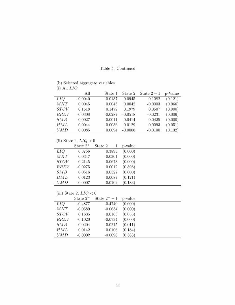
Table 5: Continued

(b) Selected aggregate variables(i) All LIQ

All State 1 State 2 State 2 − 1 p-Value

LIQ -0.0040 -0.0137 0.0945 0.1082 (0.121)MKT 0.0045 0.0045 0.0042 -0.0003 (0.966)STOV 0.1518 0.1472 0.1979 0.0507 (0.000)RREV -0.0308 -0.0287 -0.0518 -0.0231 (0.006)SMB 0.0027 -0.0011 0.0414 0.0425 (0.000)HML 0.0044 0.0036 0.0129 0.0093 (0.051)UMD 0.0085 0.0094 -0.0006 -0.0100 (0.132)

(ii) State 2, LIQ > 0State 2+ State 2+ − 1 p-value

LIQ 0.3756 0.3893 (0.000)MKT 0.0347 0.0301 (0.000)STOV 0.2145 0.0673 (0.000)RREV -0.0275 0.0012 (0.898)SMB 0.0516 0.0527 (0.000)HML 0.0123 0.0087 (0.121)UMD -0.0007 -0.0102 (0.183)

(iii) State 2, LIQ < 0State 2− State 2− − 1 p-value

LIQ -0.4877 -0.4740 (0.000)MKT -0.0589 -0.0634 (0.000)STOV 0.1635 0.0163 (0.055)RREV -0.1020 -0.0734 (0.000)SMB 0.0204 0.0215 (0.011)HML 0.0142 0.0106 (0.184)UMD -0.0002 -0.0096 (0.363)

44

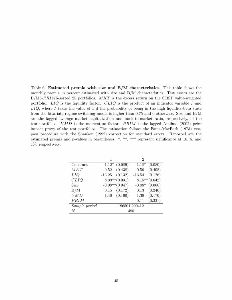
Table 6: Estimated premia with size and B/M characteristics. This table shows themonthly premia in percent estimated with size and B/M characteristics. Test assets are theB/M5-PRIM5-sorted 25 portfolios. MKT is the excess return on the CRSP value-weightedportfolio. LIQ is the liquidity factor. CLIQ is the product of an indicator variable I andLIQ, where I takes the value of 1 if the probability of being in the high liquidity-beta statefrom the bivariate regime-switching model is higher than 0.75 and 0 otherwise. Size and B/Mare the lagged average market capitalization and book-to-market ratio, respectively, of thetest portfolios. UMD is the momentum factor. PRIM is the lagged Amihud (2002) priceimpact proxy of the test portfolios. The estimation follows the Fama-MacBeth (1973) two-pass procedure with the Shanken (1992) correction for standard errors. Reported are theestimated premia and p-values in parentheses. *, **, *** represent significance at 10, 5, and1%, respectively.

1 2

Constant 1.12* (0.089) 1.18* (0.080)MKT -0.52 (0.438) -0.56 (0.408)LIQ -13.25 (0.132) -13.54 (0.126)CLIQ 8.09**(0.031) 8.15**(0.042)Size -0.08**(0.047) -0.08* (0.060)B/M 0.15 (0.172) 0.13 (0.246)UMD 1.46 (0.160) 1.39 (0.176)PRIM 0.11 (0.221)

Sample period 196501:200412N 480

45

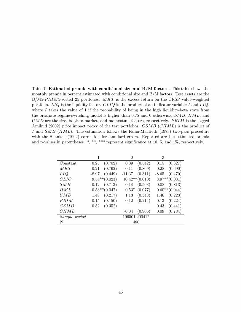
Table 7: Estimated premia with conditional size and B/M factors. This table shows themonthly premia in percent estimated with conditional size and B/M factors. Test assets are theB/M5-PRIM5-sorted 25 portfolios. MKT is the excess return on the CRSP value-weightedportfolio. LIQ is the liquidity factor. CLIQ is the product of an indicator variable I and LIQ,where I takes the value of 1 if the probability of being in the high liquidity-beta state fromthe bivariate regime-switching model is higher than 0.75 and 0 otherwise. SMB, HML, andUMD are the size, book-to-market, and momentum factors, respectively. PRIM is the laggedAmihud (2002) price impact proxy of the test portfolios. CSMB (CHML) is the product ofI and SMB (HML). The estimation follows the Fama-MacBeth (1973) two-pass procedurewith the Shanken (1992) correction for standard errors. Reported are the estimated premiaand p-values in parentheses. *, **, *** represent significance at 10, 5, and 1%, respectively.

1 2 3

Constant 0.25 (0.702) 0.39 (0.542) 0.15 (0.827)MKT 0.21 (0.762) 0.11 (0.869) 0.28 (0.690)LIQ -8.97 (0.449) -11.37 (0.311) -8.65 (0.470)CLIQ 9.54**(0.023) 10.42**(0.010) 8.97**(0.031)SMB 0.12 (0.713) 0.18 (0.563) 0.08 (0.813)HML 0.58**(0.047) 0.53* (0.077) 0.60**(0.044)UMD 1.48 (0.217) 1.13 (0.348) 1.46 (0.223)PRIM 0.15 (0.150) 0.12 (0.214) 0.13 (0.224)CSMB 0.52 (0.352) 0.43 (0.441)CHML -0.04 (0.906) 0.09 (0.784)

Sample period 196501:200412N 480

46

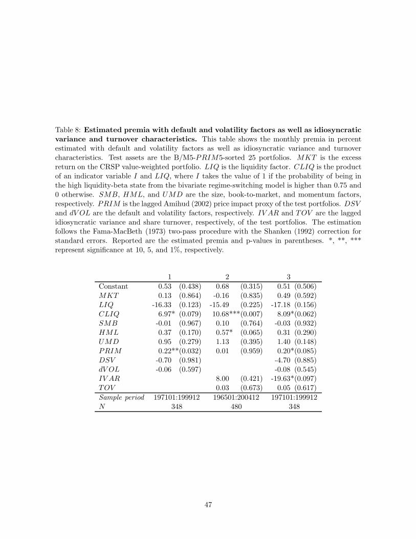
Table 8: Estimated premia with default and volatility factors as well as idiosyncraticvariance and turnover characteristics. This table shows the monthly premia in percentestimated with default and volatility factors as well as idiosyncratic variance and turnovercharacteristics. Test assets are the B/M5-PRIM5-sorted 25 portfolios. MKT is the excessreturn on the CRSP value-weighted portfolio. LIQ is the liquidity factor. CLIQ is the productof an indicator variable I and LIQ, where I takes the value of 1 if the probability of being inthe high liquidity-beta state from the bivariate regime-switching model is higher than 0.75 and0 otherwise. SMB, HML, and UMD are the size, book-to-market, and momentum factors,respectively. PRIM is the lagged Amihud (2002) price impact proxy of the test portfolios. DSVand dV OL are the default and volatility factors, respectively. IV AR and TOV are the laggedidiosyncratic variance and share turnover, respectively, of the test portfolios. The estimationfollows the Fama-MacBeth (1973) two-pass procedure with the Shanken (1992) correction forstandard errors. Reported are the estimated premia and p-values in parentheses. *, **, ***represent significance at 10, 5, and 1%, respectively.

1 2 3

Constant 0.53 (0.438) 0.68 (0.315) 0.51 (0.506)MKT 0.13 (0.864) -0.16 (0.835) 0.49 (0.592)LIQ -16.33 (0.123) -15.49 (0.225) -17.18 (0.156)CLIQ 6.97* (0.079) 10.68***(0.007) 8.09*(0.062)SMB -0.01 (0.967) 0.10 (0.764) -0.03 (0.932)HML 0.37 (0.170) 0.57* (0.065) 0.31 (0.290)UMD 0.95 (0.279) 1.13 (0.395) 1.40 (0.148)PRIM 0.22**(0.032) 0.01 (0.959) 0.20*(0.085)DSV -0.70 (0.981) -4.70 (0.885)dV OL -0.06 (0.597) -0.08 (0.545)IV AR 8.00 (0.421) -19.63*(0.097)TOV 0.03 (0.673) 0.05 (0.617)

Sample period 197101:199912 196501:200412 197101:199912N 348 480 348

47

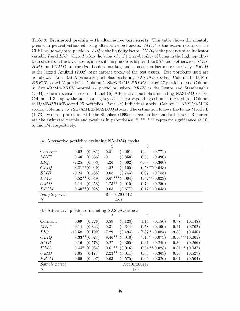
Table 9: Estimated premia with alternative test assets. This table shows the monthlypremia in percent estimated using alternative test assets. MKT is the excess return on theCRSP value-weighted portfolio. LIQ is the liquidity factor. CLIQ is the product of an indicatorvariable I and LIQ, where I takes the value of 1 if the probability of being in the high liquidity-beta state from the bivariate regime-switching model is higher than 0.75 and 0 otherwise. SMB,HML, and UMD are the size, book-to-market, and momentum factors, respectively. PRIMis the lagged Amihud (2002) price impact proxy of the test assets. Test portfolios used areas follows: Panel (a) Alternative portfolios excluding NASDAQ stocks. Column 1: B/M5-RREV 5-sorted 25 portfolios, Column 2: Size3-B/M3-PRIM3-sorted 27 portfolios, and Column3: Size3-B/M3-RREV 3-sorted 27 portfolios, where RREV is the Pastor and Stambaugh’s(2003) return reversal measure. Panel (b) Alternative portfolios including NASDAQ stocks.Columns 1-3 employ the same sorting keys as the corresponding columns in Panel (a). Column4: B/M5-PRIM5-sorted 25 portfolios. Panel (c) Individual stocks. Column 1: NYSE/AMEXstocks, Column 2: NYSE/AMEX/NASDAQ stocks. The estimation follows the Fama-MacBeth(1973) two-pass procedure with the Shanken (1992) correction for standard errors. Reportedare the estimated premia and p-values in parentheses. *, **, *** represent significance at 10,5, and 1%, respectively.

(a) Alternative portfolios excluding NASDAQ stocks1 2 3

Constant 0.02 (0.981) 0.51 (0.291) -0.20 (0.772)MKT 0.40 (0.566) -0.11 (0.850) 0.65 (0.390)LIQ -7.25 (0.353) 4.26 (0.602) -7.09 (0.360)CLIQ 8.81**(0.049) 4.52 (0.105) 6.58**(0.043)SMB -0.24 (0.435) 0.08 (0.743) 0.07 (0.785)HML 0.52**(0.049) 0.67***(0.004) 0.52**(0.029)UMD 1.14 (0.258) 1.73** (0.015) 0.79 (0.250)PRIM 0.30**(0.028) 0.05 (0.577) 0.17**(0.045)

Sample period 196501:200412N 480

(b) Alternative portfolios including NASDAQ stocks1 2 3 4

Constant 0.69 (0.226) 0.89 (0.128) 1.14 (0.156) 0.78 (0.148)MKT -0.14 (0.823) -0.31 (0.644) -0.58 (0.490) -0.24 (0.702)LIQ -10.58 (0.192) -7.29 (0.494) -17.37* (0.084) -9.88 (0.446)CLIQ 9.33**(0.027) 9.46** (0.010) 7.16* (0.073) 10.50***(0.005)SMB 0.16 (0.578) 0.27 (0.305) 0.31 (0.249) 0.30 (0.266)HML 0.44* (0.064) 0.61** (0.016) 0.54**(0.023) 0.51** (0.037)UMD 1.05 (0.177) 2.23** (0.011) 0.66 (0.363) 0.50 (0.527)PRIM 0.09 (0.297) -0.03 (0.575) 0.06 (0.326) 0.04 (0.504)

Sample period 196501:200412N 480

48

Table 9: Continued

(c) Individual stocks1 2

Constant 1.72** (0.011) 2.15***(0.010)MKT -1.06 (0.193) -1.46 (0.163)LIQ -20.66* (0.082) -30.84** (0.048)CLIQ 11.94** (0.014) 12.44** (0.010)SMB 0.40 (0.224) 0.47 (0.246)HML 0.53 (0.136) 0.67 (0.184)UMD 1.19 (0.397) 1.37 (0.420)PRIM -0.09***(0.000) -0.09***(0.000)

Sample period 196501:200412N 480

49

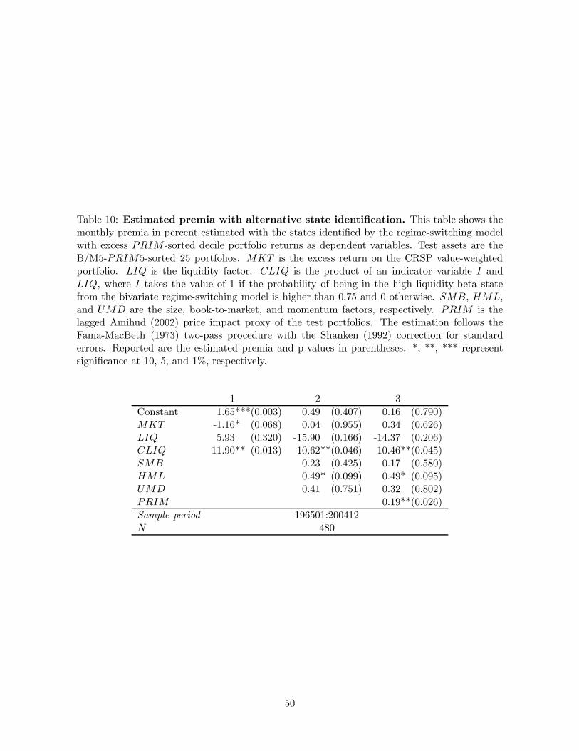
Table 10: Estimated premia with alternative state identification. This table shows themonthly premia in percent estimated with the states identified by the regime-switching modelwith excess PRIM -sorted decile portfolio returns as dependent variables. Test assets are theB/M5-PRIM5-sorted 25 portfolios. MKT is the excess return on the CRSP value-weightedportfolio. LIQ is the liquidity factor. CLIQ is the product of an indicator variable I andLIQ, where I takes the value of 1 if the probability of being in the high liquidity-beta statefrom the bivariate regime-switching model is higher than 0.75 and 0 otherwise. SMB, HML,and UMD are the size, book-to-market, and momentum factors, respectively. PRIM is thelagged Amihud (2002) price impact proxy of the test portfolios. The estimation follows theFama-MacBeth (1973) two-pass procedure with the Shanken (1992) correction for standarderrors. Reported are the estimated premia and p-values in parentheses. *, **, *** representsignificance at 10, 5, and 1%, respectively.

1 2 3

Constant 1.65***(0.003) 0.49 (0.407) 0.16 (0.790)MKT -1.16* (0.068) 0.04 (0.955) 0.34 (0.626)LIQ 5.93 (0.320) -15.90 (0.166) -14.37 (0.206)CLIQ 11.90** (0.013) 10.62**(0.046) 10.46**(0.045)SMB 0.23 (0.425) 0.17 (0.580)HML 0.49* (0.099) 0.49* (0.095)UMD 0.41 (0.751) 0.32 (0.802)PRIM 0.19**(0.026)

Sample period 196501:200412N 480

50

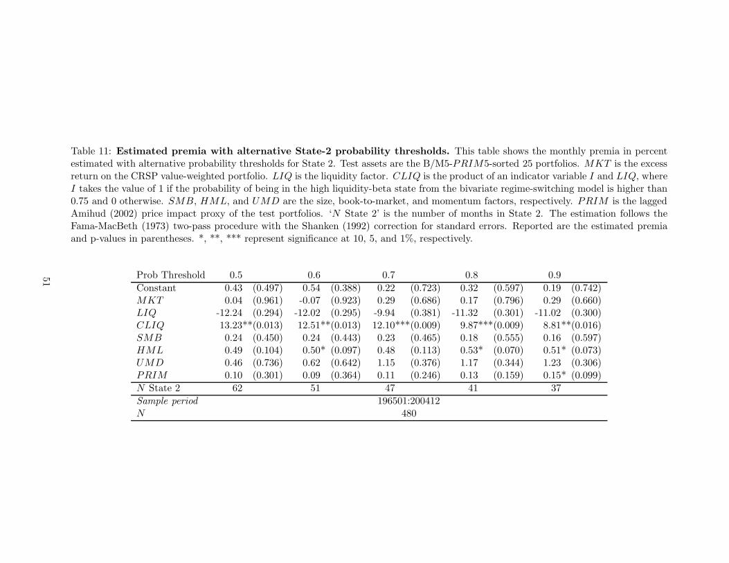
Table 11: Estimated premia with alternative State-2 probability thresholds. This table shows the monthly premia in percentestimated with alternative probability thresholds for State 2. Test assets are the B/M5-PRIM5-sorted 25 portfolios. MKT is the excessreturn on the CRSP value-weighted portfolio. LIQ is the liquidity factor. CLIQ is the product of an indicator variable I and LIQ, whereI takes the value of 1 if the probability of being in the high liquidity-beta state from the bivariate regime-switching model is higher than0.75 and 0 otherwise. SMB, HML, and UMD are the size, book-to-market, and momentum factors, respectively. PRIM is the laggedAmihud (2002) price impact proxy of the test portfolios. ‘N State 2’ is the number of months in State 2. The estimation follows theFama-MacBeth (1973) two-pass procedure with the Shanken (1992) correction for standard errors. Reported are the estimated premiaand p-values in parentheses. *, **, *** represent significance at 10, 5, and 1%, respectively.

Prob Threshold 0.5 0.6 0.7 0.8 0.9

Constant 0.43 (0.497) 0.54 (0.388) 0.22 (0.723) 0.32 (0.597) 0.19 (0.742)MKT 0.04 (0.961) -0.07 (0.923) 0.29 (0.686) 0.17 (0.796) 0.29 (0.660)LIQ -12.24 (0.294) -12.02 (0.295) -9.94 (0.381) -11.32 (0.301) -11.02 (0.300)CLIQ 13.23**(0.013) 12.51**(0.013) 12.10***(0.009) 9.87***(0.009) 8.81**(0.016)SMB 0.24 (0.450) 0.24 (0.443) 0.23 (0.465) 0.18 (0.555) 0.16 (0.597)HML 0.49 (0.104) 0.50* (0.097) 0.48 (0.113) 0.53* (0.070) 0.51* (0.073)UMD 0.46 (0.736) 0.62 (0.642) 1.15 (0.376) 1.17 (0.344) 1.23 (0.306)PRIM 0.10 (0.301) 0.09 (0.364) 0.11 (0.246) 0.13 (0.159) 0.15* (0.099)

N State 2 62 51 47 41 37

Sample period 196501:200412N 480

51

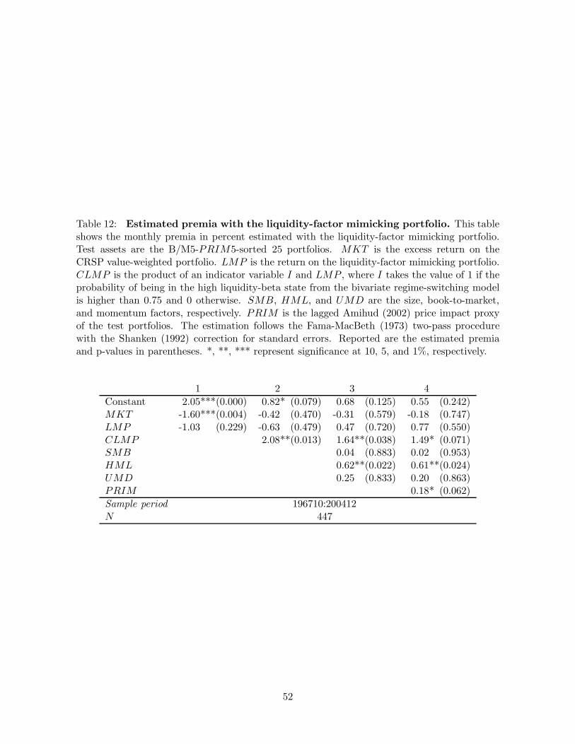
Table 12: Estimated premia with the liquidity-factor mimicking portfolio. This tableshows the monthly premia in percent estimated with the liquidity-factor mimicking portfolio.Test assets are the B/M5-PRIM5-sorted 25 portfolios. MKT is the excess return on theCRSP value-weighted portfolio. LMP is the return on the liquidity-factor mimicking portfolio.CLMP is the product of an indicator variable I and LMP , where I takes the value of 1 if theprobability of being in the high liquidity-beta state from the bivariate regime-switching modelis higher than 0.75 and 0 otherwise. SMB, HML, and UMD are the size, book-to-market,and momentum factors, respectively. PRIM is the lagged Amihud (2002) price impact proxyof the test portfolios. The estimation follows the Fama-MacBeth (1973) two-pass procedurewith the Shanken (1992) correction for standard errors. Reported are the estimated premiaand p-values in parentheses. *, **, *** represent significance at 10, 5, and 1%, respectively.

1 2 3 4

Constant 2.05***(0.000) 0.82* (0.079) 0.68 (0.125) 0.55 (0.242)MKT -1.60***(0.004) -0.42 (0.470) -0.31 (0.579) -0.18 (0.747)LMP -1.03 (0.229) -0.63 (0.479) 0.47 (0.720) 0.77 (0.550)CLMP 2.08**(0.013) 1.64**(0.038) 1.49* (0.071)SMB 0.04 (0.883) 0.02 (0.953)HML 0.62**(0.022) 0.61**(0.024)UMD 0.25 (0.833) 0.20 (0.863)PRIM 0.18* (0.062)

Sample period 196710:200412N 447

52

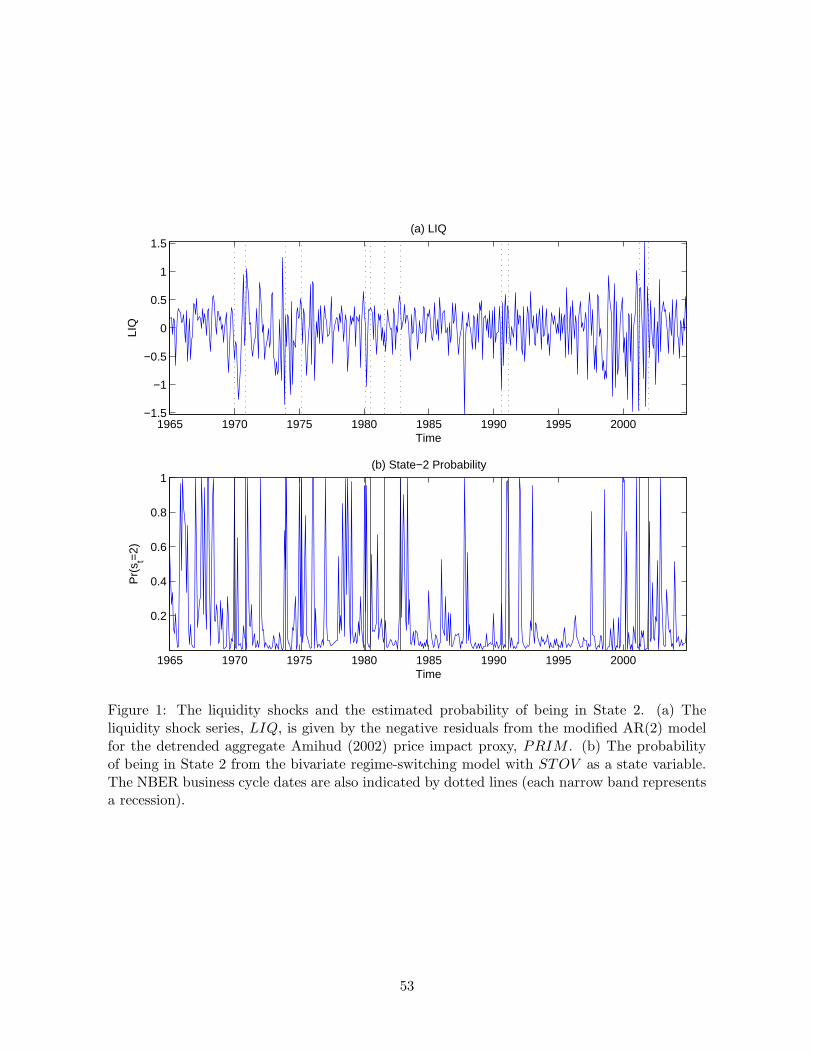
1965 1970 1975 1980 1985 1990 1995 2000−1.5

−1

−0.5

0

0.5

1

1.5(a) LIQ

Time

LIQ

1965 1970 1975 1980 1985 1990 1995 2000

0.2

0.4

0.6

0.8

1(b) State−2 Probability

Time

Pr(

s t=2)

Figure 1: The liquidity shocks and the estimated probability of being in State 2. (a) Theliquidity shock series, LIQ, is given by the negative residuals from the modified AR(2) modelfor the detrended aggregate Amihud (2002) price impact proxy, PRIM . (b) The probabilityof being in State 2 from the bivariate regime-switching model with STOV as a state variable.The NBER business cycle dates are also indicated by dotted lines (each narrow band representsa recession).

53

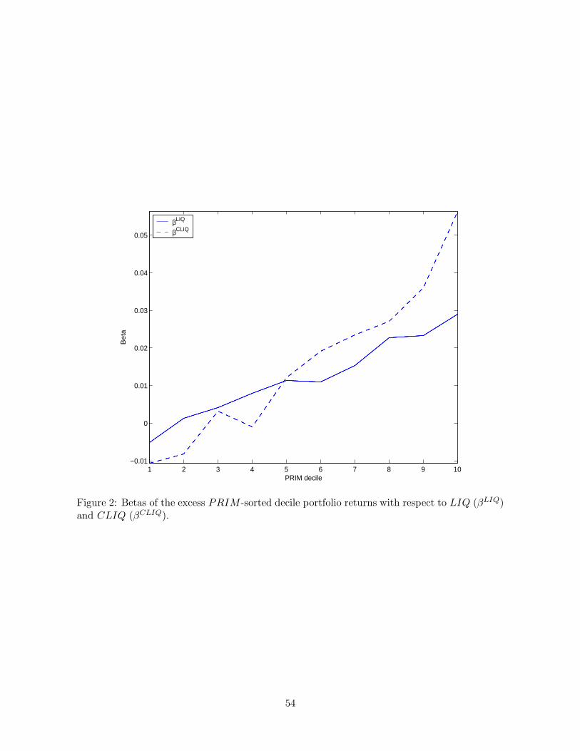
1 2 3 4 5 6 7 8 9 10−0.01

0

0.01

0.02

0.03

0.04

0.05

PRIM decile

Bet

a

βLIQ

βCLIQ

Figure 2: Betas of the excess PRIM -sorted decile portfolio returns with respect to LIQ (βLIQ)and CLIQ (βCLIQ).

54

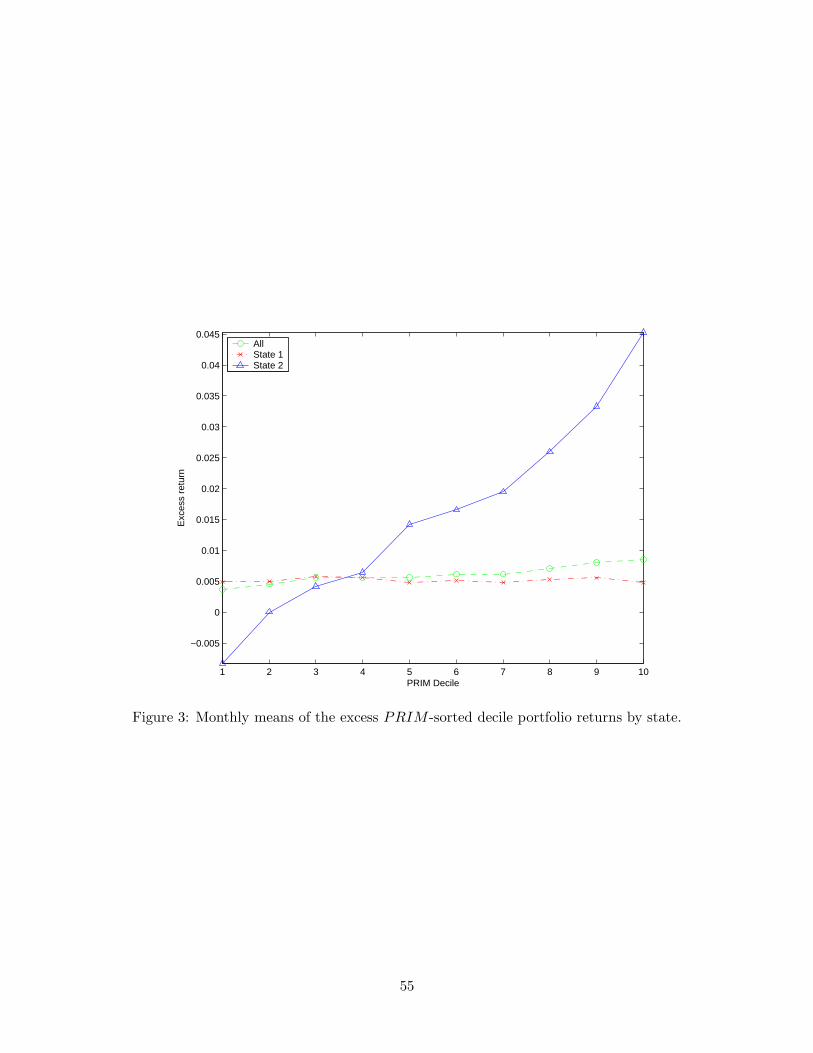
1 2 3 4 5 6 7 8 9 10

−0.005

0

0.005

0.01

0.015

0.02

0.025

0.03

0.035

0.04

0.045

PRIM Decile

Exc

ess

retu

rn

AllState 1State 2

Figure 3: Monthly means of the excess PRIM -sorted decile portfolio returns by state.

55

−4 −3 −2 −1 0 1 2 3 4−0.02

0

0.02

0.04

0.06

0.08

0.1

Ret

urn

−4 −3 −2 −1 0 1 2 3 4−0.2

−0.1

0

0.1

0.2

0.3

0.4

0.5(a) State 2, LIQ>0

Months to State 2

LIQ

PRIM01 (L)PRIM03 (L)PRIM05 (L)PRIM08 (L)PRIM10 (L)LIQ (R)

−4 −3 −2 −1 0 1 2 3 4−0.08

−0.06

−0.04

−0.02

0

0.02

0.04

Ret

urn

−4 −3 −2 −1 0 1 2 3 4−0.5

−0.4

−0.3

−0.2

−0.1

0

0.1

0.2(b) State 2, LIQ<0

Months to State 2

LIQ

Figure 4: Average raw returns of selected PRIM -sorted decile portfolios (left scale) and LIQ(right scale) conditional on the sign of LIQ in State 2. PRIM01 represents the lowest PRIMdecile and PRIM10 the highest. The horizontal axis is the number of months to State 2.

56

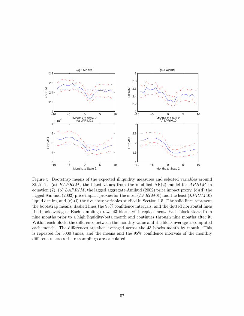
−10 −5 0 5 102

2.2

2.4

2.6

2.8(a) EAPRIM

EA

PR

IM

Months to State 2−10 −5 0 5 102

2.2

2.4

2.6

2.8

3(b) LAPRIM

LAP

RIM

Months to State 2

−10 −5 0 5 103

4

5

6

7x 10

−3 (c) LPRIM01

LPR

IM01

Months to State 2−10 −5 0 5 101

1.5

2

2.5

3(d) LPRIM10

LPR

IM10

Months to State 2

Figure 5: Bootstrap means of the expected illiquidity measures and selected variables aroundState 2. (a) EAPRIM , the fitted values from the modified AR(2) model for APRIM inequation (7), (b) LAPRIM , the lagged aggregate Amihud (2002) price impact proxy, (c)(d) thelagged Amihud (2002) price impact proxies for the most (LPRIM01) and the least (LPRIM10)liquid deciles, and (e)-(i) the five state variables studied in Section 1.5. The solid lines representthe bootstrap means, dashed lines the 95% confidence intervals, and the dotted horizontal linesthe block averages. Each sampling draws 43 blocks with replacement. Each block starts fromnine months prior to a high liquidity-beta month and continues through nine months after it.Within each block, the difference between the monthly value and the block average is computedeach month. The differences are then averaged across the 43 blocks month by month. Thisis repeated for 5000 times, and the means and the 95% confidence intervals of the monthlydifferences across the re-samplings are calculated.

57

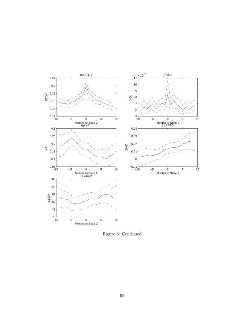
−10 −5 0 5 100.12

0.14

0.16

0.18

0.2

0.22(e) STOV

ST

OV

Months to State 2−10 −5 0 5 105

6

7

8

9

10

11x 10

−3 (f) VOL

VO

L

Months to State 2

−10 −5 0 5 100.05

0.1

0.15

0.2

0.25

0.3(g) XRI

XR

I

Months to State 2−10 −5 0 5 10

−0.01

0

0.01

0.02

0.03

0.04(h) LEAD

LEA

D

Months to State 2

−10 −5 0 5 1076

78

80

82

84

86(i) CEXP

CE

XP

Months to State 2

Figure 5: Continued

58