time series analysis - lecture 3 forecasting using arima-models step 1. assess the stationarity of...
Post on 19-Dec-2015
216 views
TRANSCRIPT

Time series analysis - lecture 3
Forecasting using ARIMA-models
Step 1. Assess the stationarity of the given time series of data and form differences if necessary
Step 2. Estimate auto-correlations and partial auto-correlations, and select a suitable ARMA-model
Step 3. Compute forecasts according to the estimated model
Time series analysis - lecture 3
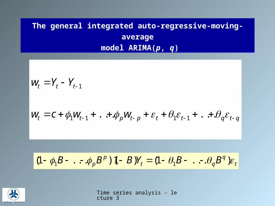
The general integrated auto-regressive-moving-average
model ARIMA(p, q)
qtqttptptt
ttt
wwcw
YYw
...... 1111
1
tq
qtp
p BBYBBB )...1()1)(...1( 11
Time series analysis - lecture 3
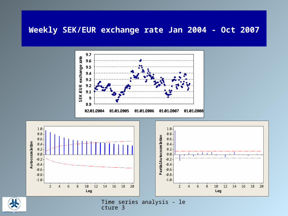
Weekly SEK/EUR exchange rate Jan 2004 - Oct 2007
8.9
9
9.1
9.2
9.3
9.4
9.5
9.6
9.7
02/01/2004 01/01/2005 01/01/2006 01/01/2007 01/01/2008
SE
K/E
UR
exc
han
ge
rate
2018161412108642
1.00.80.60.40.20.0
-0.2-0.4-0.6-0.8-1.0
Lag
Auto
corr
ela
tion
2018161412108642
1.00.80.60.40.20.0
-0.2-0.4-0.6-0.8-1.0
Lag
Part
ial A
uto
corr
ela
tion
Time series analysis - lecture 3
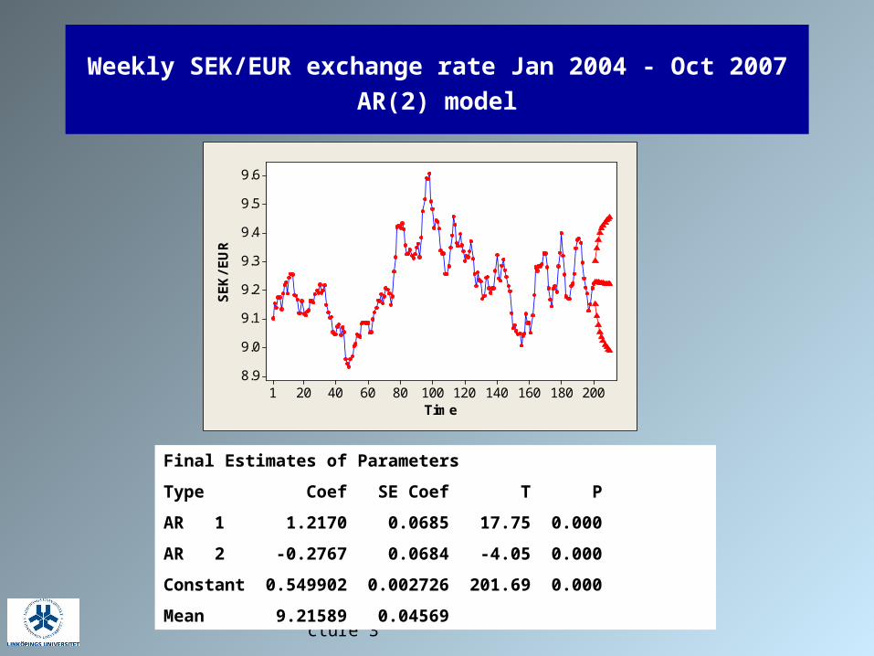
Weekly SEK/EUR exchange rate Jan 2004 - Oct 2007
AR(2) model
Final Estimates of Parameters
Type Coef SE Coef T P
AR 1 1.2170 0.0685 17.75 0.000
AR 2 -0.2767 0.0684 -4.05 0.000
Constant 0.549902 0.002726 201.69 0.000
Mean 9.21589 0.04569
200180160140120100806040201
9.6
9.5
9.4
9.3
9.2
9.1
9.0
8.9
Time
SEK
/EU
R
Time series analysis - lecture 3
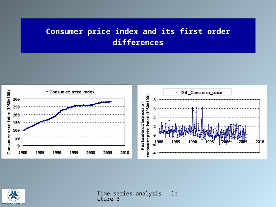
Consumer price index and its first order differences
0
50
100
150
200
250
300
1980 1985 1990 1995 2000 2005 2010Co
nsu
mer
pri
ce in
dex
(19
80=
100) Consumer_price_index
-4
-2
0
2
4
6
8
1980 1985 1990 1995 2000 2005 2010F
irst
ord
er d
iffe
ren
ces
of
con
sum
er p
rice
ind
ex (
1980
=10
0)
Diff_Consumer_price
Time series analysis - lecture 3
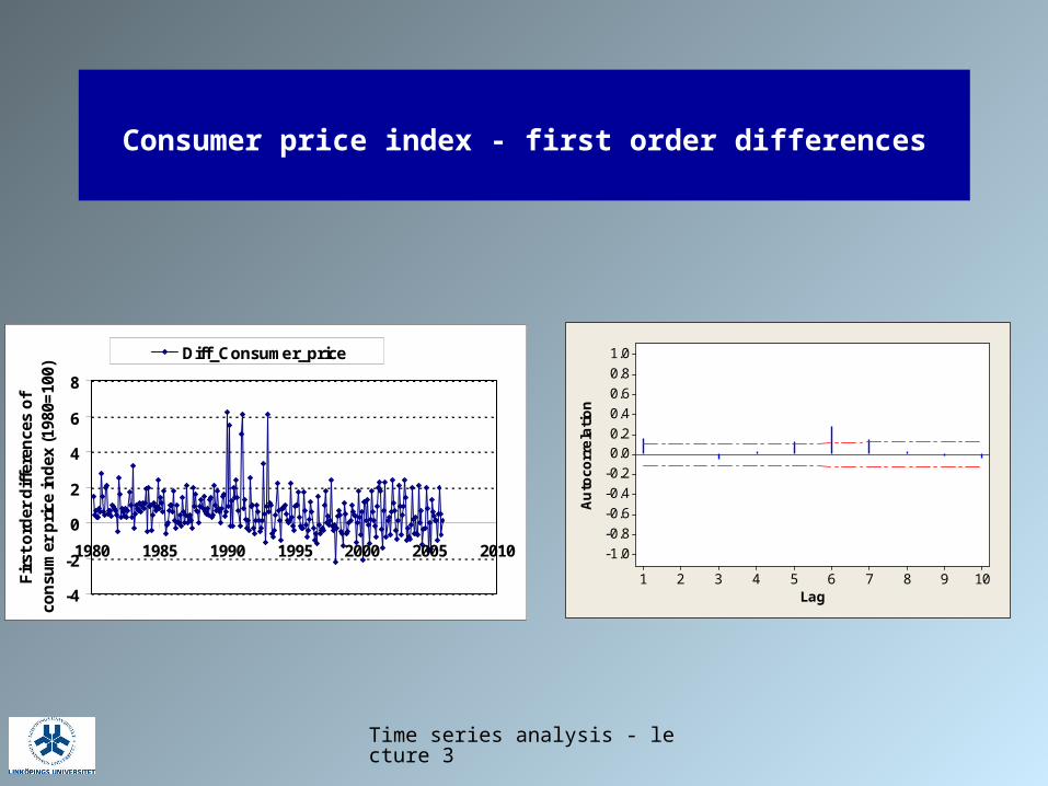
Consumer price index - first order differences
10987654321
1.00.80.60.40.20.0
-0.2-0.4-0.6-0.8-1.0
LagAuto
corr
ela
tion
-4
-2
0
2
4
6
8
1980 1985 1990 1995 2000 2005 2010
Fir
st o
rder
dif
fere
nce
s o
f co
nsu
mer
pri
ce in
dex
(19
80=
100)
Diff_Consumer_price
Time series analysis - lecture 3
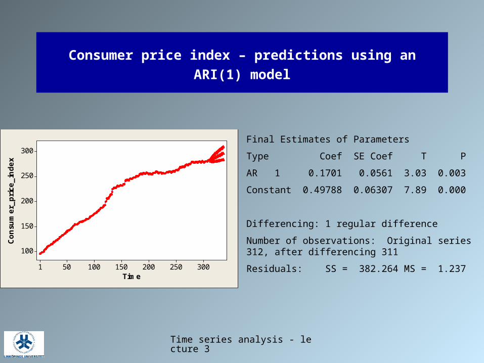
Consumer price index – predictions using an ARI(1) model
300250200150100501
300
250
200
150
100
Time
Consu
mer_
pri
ce_in
dex
Final Estimates of Parameters
Type Coef SE Coef T P
AR 1 0.1701 0.0561 3.03 0.003
Constant 0.49788 0.06307 7.89 0.000
Differencing: 1 regular difference
Number of observations: Original series 312, after differencing 311
Residuals: SS = 382.264 MS = 1.237

Time series analysis - lecture 3
Seasonal differencing
Form
where S depicts the seasonal length
tS
Sttt YBYYw )1(

Time series analysis - lecture 3
Consumer price index and its seasonal differences
-5
0
5
10
15
20
25
30
1980 1985 1990 1995 2000 2005 2010S
easo
nal
dif
fere
nce
s o
f co
nsu
mer
pri
ce in
dex
(19
80=
100)
Seasonal diff
0
50
100
150
200
250
300
1980 1985 1990 1995 2000 2005 2010Co
nsu
mer
pri
ce in
dex
(19
80=
100) Consumer_price_index
Time series analysis - lecture 3
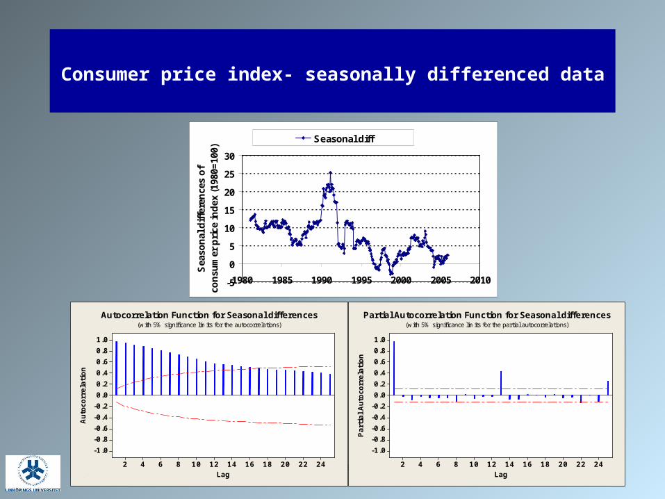
Consumer price index- seasonally differenced data
24222018161412108642
1.0
0.8
0.6
0.4
0.2
0.0
-0.2
-0.4
-0.6
-0.8
-1.0
Lag
Auto
corr
ela
tion
Autocorrelation Function for Seasonal differences(with 5% significance limits for the autocorrelations)
-5
0
5
10
15
20
25
30
1980 1985 1990 1995 2000 2005 2010
Sea
son
al d
iffe
ren
ces
of
con
sum
er p
rice
ind
ex (
1980
=10
0)
Seasonal diff
24222018161412108642
1.0
0.8
0.6
0.4
0.2
0.0
-0.2
-0.4
-0.6
-0.8
-1.0
Lag
Part
ial Auto
corr
ela
tion
Partial Autocorrelation Function for Seasonal differences(with 5% significance limits for the partial autocorrelations)

Time series analysis - lecture 3
Consumer price index- differenced and seasonally differenced data
-8
-6
-4
-2
0
2
4
6
8
1980 1985 1990 1995 2000 2005 2010
Dif
fere
nce
s o
f se
aso
nal
dif
fere
nce
s o
f co
nsu
mer
pri
ce i
nd
ex
(198
0=10
0)
Diff. and seasonally diff.
24222018161412108642
1.0
0.8
0.6
0.4
0.2
0.0
-0.2
-0.4
-0.6
-0.8
-1.0
Lag
Auto
corr
ela
tion
Autocorrelation Function for Diff. of seasonal diff.(with 5% significance limits for the autocorrelations)
24222018161412108642
1.0
0.8
0.6
0.4
0.2
0.0
-0.2
-0.4
-0.6
-0.8
-1.0
Lag
Part
ial Auto
corr
ela
tion
Partial Autocorrelation Function for Diff. of seasonal diff.(with 5% significance limits for the partial autocorrelations)
Time series analysis - lecture 3
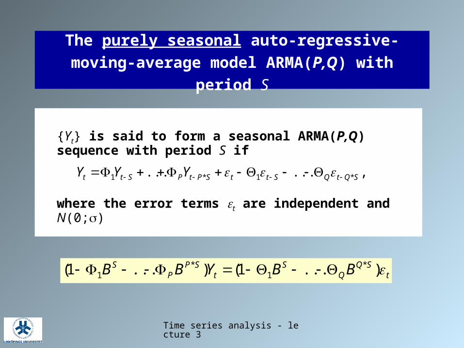
The purely seasonal auto-regressive-moving-
average model ARMA(P,Q) with period S
{Yt} is said to form a seasonal ARMA(P,Q) sequence with period S if
where the error terms t are independent and N(0;)
,...... *1*1 SQtQSttSPtPStt YYY
tSQ
QS
tSP
PS BBYBB )...1()...1( *
1*
1

Time series analysis - lecture 3
Typical auto-correlation functions of purely
seasonal ARMA(P,Q) sequences with period S
Auto-correlations are non-zero only at lags S, 2S, 3S, …
In addition: AR(P): Autocorrelations tail off gradually with increasing time-lags
MA(Q): Auto-correlations are zero for time lags greater than q*S
ARMA(P,Q): Auto-correlations tail off gradually with time-lags greater than q*S

Time series analysis - lecture 3
No. air passengers by week in Sweden
-original series and seasonally differenced data
12.2
12.4
12.6
12.8
13.0
13.2
13.4
13.6
1992 1996 2000 2004No
.pas
sen
ger
s at
Sw
edis
h a
irp
ort
s (t
ho
usa
nd
s)
No. passengers
-0.4
-0.3
-0.2
-0.1
0.0
0.1
0.2
0.3
0.4
1992 1996 2000 2004D
iffe
ren
ce la
g 5
2 (t
ho
usa
nd
s)
Difference lag 52
Time series analysis - lecture 3
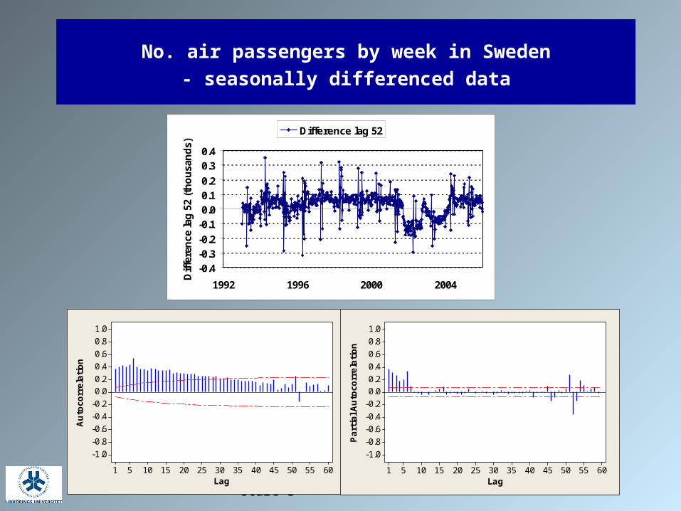
No. air passengers by week in Sweden
- seasonally differenced data
-0.4
-0.3
-0.2
-0.1
0.0
0.1
0.2
0.3
0.4
1992 1996 2000 2004
Dif
fere
nce
lag
52
(th
ou
san
ds)
Difference lag 52
605550454035302520151051
1.00.80.60.40.20.0
-0.2-0.4-0.6-0.8-1.0
Lag
Auto
corr
ela
tion
605550454035302520151051
1.00.80.60.40.20.0
-0.2-0.4-0.6-0.8-1.0
Lag
Part
ial A
uto
corr
ela
tion
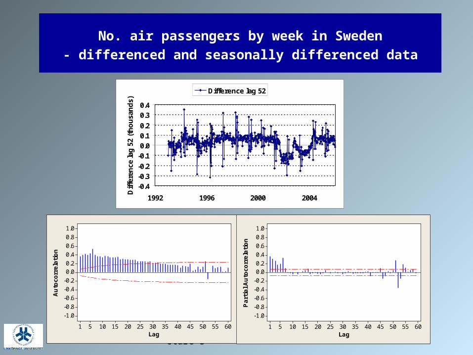
Time series analysis - lecture 3
No. air passengers by week in Sweden
- differenced and seasonally differenced data
-0.4
-0.3
-0.2
-0.1
0.0
0.1
0.2
0.3
0.4
1992 1996 2000 2004
Dif
fere
nce
lag
52
(th
ou
san
ds)
Difference lag 52
605550454035302520151051
1.00.80.60.40.20.0
-0.2-0.4-0.6-0.8-1.0
Lag
Auto
corr
ela
tion
605550454035302520151051
1.00.80.60.40.20.0
-0.2-0.4-0.6-0.8-1.0
Lag
Part
ial A
uto
corr
ela
tion

Time series analysis - lecture 3
The general seasonal auto-regressive-moving-
average model ARMA(p, q, P, Q) with period S
{Yt} is said to form a seasonal ARMA(p, q, P, Q) sequence with period S if
where the error terms t are independent and N(0;)
Example: p = P = 0, q = Q = 1, S = 12
.
131112111112
1 )1)(1( tttttt BBY
tq
qSQ
QS
tp
pSP
PS
BBBB
YBBBB
)...1)(...1(
)...1)(...1(
1*
1
1*
1

Time series analysis - lecture 3
The general seasonal integrated auto-regressive-moving-
average model ARMA(p, q, P, Q) with period S
{Yt} is said to form a seasonal ARIMA(p, q, d, P, Q, D) sequence with period S if
where the error terms t are independent and N(0;)
tq
qSQ
QS
tdDSp
pSP
PS
BBBB
YBBBBBB
)...1)(...1(
)1()1)(...1)(...1(
1*
1
1*
1

Time series analysis - lecture 3
Forecasting using Seasonal ARIMA-models
Step 1. Assess the stationarity of the given time series of data and form differences and seasonal differences if necessary
Step 2. Estimate auto-correlations and partial auto-correlations, and select a suitable ARMA-model of the short-term dependence
Step 3. Estimate auto-correlations and partial auto-correlations, and select a suitable seasonal ARMA-model of the variation by season
Step 4. Compute forecasts according to the estimated model

Time series analysis - lecture 3
Consumer price index- differenced and seasonally differenced data
-8
-6
-4
-2
0
2
4
6
8
1980 1985 1990 1995 2000 2005 2010
Dif
fere
nce
s o
f se
aso
nal
dif
fere
nce
s o
f co
nsu
mer
pri
ce i
nd
ex
(198
0=10
0)
Diff. and seasonally diff.
24222018161412108642
1.0
0.8
0.6
0.4
0.2
0.0
-0.2
-0.4
-0.6
-0.8
-1.0
Lag
Auto
corr
ela
tion
Autocorrelation Function for Diff. of seasonal diff.(with 5% significance limits for the autocorrelations)
24222018161412108642
1.0
0.8
0.6
0.4
0.2
0.0
-0.2
-0.4
-0.6
-0.8
-1.0
Lag
Part
ial Auto
corr
ela
tion
Partial Autocorrelation Function for Diff. of seasonal diff.(with 5% significance limits for the partial autocorrelations)
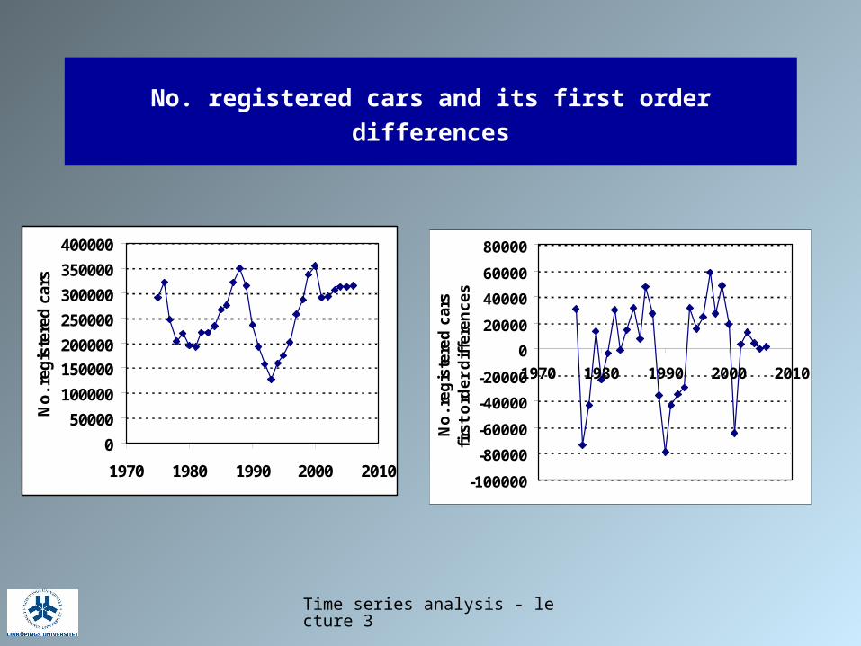
Time series analysis - lecture 3
No. registered cars and its first order differences
0
50000
100000
150000
200000
250000
300000
350000
400000
1970 1980 1990 2000 2010
No
. reg
iste
red
car
s
-100000
-80000
-60000
-40000
-20000
0
20000
40000
60000
80000
1970 1980 1990 2000 2010
No
. re
gis
tere
d c
ars
firs
t o
rde
r d
iffe
ren
ce
s

Time series analysis - lecture 3
No. registered cars
- first order differences
-100000
-80000
-60000
-40000
-20000
0
20000
40000
60000
80000
1970 1980 1990 2000 2010
No
. re
gis
tere
d c
ars
firs
t o
rde
r d
iffe
ren
ce
s
10987654321
1.00.80.60.40.20.0
-0.2-0.4-0.6-0.8-1.0
Lag
Auto
corr
ela
tion
30282624222018161412108642
1.00.80.60.40.20.0
-0.2-0.4-0.6-0.8-1.0
Lag
Part
ial A
uto
corr
ela
tion