Time of Flight Software for the CLAS12 Particle DetectorAlexander Colvill

A dissertation submitted to the Physics Department at the University of Surrey in partialfulfilment of the degree of Master in Physics.

Department of PhysicsUniversity of SurreyFebruary 2014

I Abstract

The main experimental apparatus at the Thomas Jefferson National Accelerator Facility (also

Jefferson Laboratory, or Jlab) in Newport News, Virginia is the Continuous Electron Beam

Accelerator Facility (CEBAF), which supplies beams of electrons to three experimental halls.

CEBAF is in the middle of an upgrade to increase the maximum beam energy from 5.7 to 11 GeV.

As part of this upgrade, the existing particle detector in experimental Hall B, the Continuous Large

Acceptance Spectrometer (CLAS6), is being rebuilt. The new detector, CLAS12, includes two

subsystems that measure the flight time of particles - the Central Time of Flight (CTOF) and the

Forward Time of Flight (FTOF) - built from arrays of scintillation paddles. The focus of this

research has been the development of software that processes the raw data output by these

subsystems. It is based on existing software written for the FTOF of the old detector, which is

similar, but not identical to, the FTOF in CLAS12. Written in Java, the new software will run in the

CLAS12 Reconstruction and Analysis Framework (CLARA). CLARA is based on a Service-

Oriented Architecture (SOA) and, as such, the CTOF and FTOF applications are known as software

services. Simulation of the CLAS12 detector has been used to shape the design of these services

and to test them, as well as to provide some general results as to how the TOF detectors will behave

when the CLAS12 detector is switched on in 2016. Most significantly, simulation has been used to

optimize the way that particle hits on adjacent scintillation paddles are combined into clusters. This

process is more efficient if FTOF panels are treated individually and if clusters are made from more

than 2 paddle hits. The bulk of this report describes the current state of the TOF services, the

physics behind their operation, as well as highlighting what work remains to be done.

1

II Acknowledgements

The author would like to thank Gerard Gilfoyle (University of Richmond) for his guidance

throughout this project, visiting tutors Patrick Regan and Paul Stevenson, and Jlab associates

Veronique Ziegler, Dennis Weygand, Vardan Gyurjyan, Johann Goetz, Daniel Carman, Justin Ruger,

Haiyan Lu, Maurizio Ungaro, Yelena Prok and Sebastian Mancilla.

This project was possible due to a grant from the US Department of Energy.

III List of Abbreviations

ADC Analog to Digital ConverterBMT Barrel Micromegas TrackerCEBAF Continuous Electron Beam Accelerator FacilityCLARA CLAS12 Analysis and Reconstruction FrameworkCLAS6 Old CEBAF Large Acceptance Spectrometer (defunct, 5.7 GeV max beam energy)CLAS12 New CEBAF Large Acceptance Spectrometer (being built, 11 GeV max beam

energy)CND Central Neutron DetectorCTOF Central Time Of FlightDISGEN Deep Inelastic Scattering GeneratorDC Drift ChamberEC Electromagnetic CalorimeterEVIO Event In OutFTOF Forward Time Of FlightGEANT Geometry and TrackingGEMC GEANT4 Monte-Carlo Simulation frameworkGUI Graphical User InterfaceHTCC High Threshold Cherenkov CounterLHC Large Hadron ColliderLTCC Low Threshold Cherenkov CounterPCAL Pre-shower CalorimeterPID Particle IdentificationPMT Photomultiplier TubeSLAC Stanford Linear AcceleratorSOA Service-Oriented ArchitectureSVT Silicon Vertex TrackerTDC Time to Digital ConverterXML Extensible Markup Language

2

IV Contents

I Abstract............................................................................................................................... 1 II Acknowledgements............................................................................................................. 2 III List of Abbreviations........................................................................................................... 2 IV Contents

1. Introduction......................................................................................................................... 5

2. Hardware and Physics Background2.1 CLAS12 Detector......................................................................................................... 11

2.1.1 Central Detector 2.1.1.1 Central Time of Flight (CTOF)

2.1.2 Forward Detector2.1.2.1 Forward Time of Flight (FTOF)

2.2 The Physics of Plastic Scintillators............................................................................. 18

3. Software Background3.1 Overview of Reconstruction Software......................................................................... 213.2 CLAS6 FTOF Reconstruction Software...................................................................... 24 3.3 Simulation of the CLAS12 detector: DISGEN and GEMC......................................... 27

4. Simulation Results4.1 CTOF............................................................................................................................ 29 4.2 FTOF............................................................................................................................ 32

5. CLAS12 FTOF Reconstruction Service

5.1 Overview...................................................................................................................... 375.2 Details of Software Packages....................................................................................... 43

5.2.1 Calibration5.2.2 Geometry5.2.3 Event5.2.4 Reconstruction

5.2.4.1 Overview5.2.4.2 ReverseEngineer Class5.2.4.3 PaddleReader5.2.4.4 PaddleCorrector5.2.4.5 PaddleConvertor5.2.4.6 SectorReconstruction5.2.4.7 PanelReconstructionCLAS125.2.4.8 ConfigPanelReconstructionCLAS125.2.4.9 PaddleReconstruction5.2.4.10 OutputCreator

5.3 Clustering Algorithm for CLAS12............................................................................... 515.3.1 Overview5.3.2 Description of CLAS6 Algorithm5.3.3 GEMC Clustering Reference

5.3.3.1 Concept5.3.3.2 Coding the Breach Condition

3

5.3.3.3 GEMC Clustering Reference Tests5.3.4 Efficiency of CLAS6 Algorithm5.3.5 Potential Alterations to CLAS6 Algorithm

5.2.5.1 Optimal Uncertainty Multiples per Panel5.2.5.2 Variable Cluster Size5.2.5.3 Optimal Uncertainty Multiples and Variable Cluster Size

5.3.6 Practical Considerations5.3.6.1 How Constant are the Optimal Uncertainty Multiples ?5.3.6.2 Optimal Uncertainty Multiples or Absolute Differences ?5.3.6.3 Calculating Clustering Parameters from the Constituent Hits5.3.6.4 Limit on Cluster Size5.3.6.5 Verification with Production Data

5.3.7 Proposed Defaults for CLAS12 Algorithm5.3.8 Implementation of Configurable CLAS12 Algorithm

5.4 Additional Prototyping..................................................................................................745.5 Testing........................................................................................................................... 745.6 Future Work...................................................................................................................77

6. CLAS12 CTOF Reconstruction Service

6.1 Overview.......................................................................................................................796.2 Code Differences versus FTOF.....................................................................................806.3 Testing...........................................................................................................................806.4 Future Work.................................................................................................................. 83

7. Summary..............................................................................................................................84 8. References............................................................................................................................85 9. Appendices...........................................................................................................................86

A Definition of CLAS6 Status IntegerB Format of Input EVIO Banks for the FTOF ServiceC Geometry XML for the FTOF ServiceD Proposed Calibration XML for the FTOF Service

E Format of Output EVIO Banks for the FTOF ServiceF Configurable Options of the FTOF ServiceG Format of Input EVIO Banks for the CTOF Service

H Proposed Geometry XML for the CTOF ServiceI Proposed Calibration XML for the CTOF ServiceJ Format of Output EVIO Banks for the CTOF ServiceK Configurable Options of the CTOF ServiceL DISGEN ParametersM GEMC ParametersN Values of Calibration Variables Used in Cluster TestsO Dependencies and Equivalencies FTOF versus CTOF

4

1. Introduction

Jefferson Laboratory is one of the US national laboratories. It is situated in Newport News,

Virginia and is owned by the US Department of Energy, who also funded this research. The

overarching goal of Jefferson Laboratory is to understand how quarks and gluons (collectively

known as partons) form nucleons and nuclei. The main technique used in pursuit of this goal is the

scattering of electrons from a stationary target, a technique similar to the one used in the early 20 th

century by Rutherford et al that showed the existence of the nucleus. Rutherford fired alpha

particles, with energies on the order of 10 MeV, at a gold foil target, and, using a fluorescent screen

and a microscope, counted the number of particles scattered at a given angle [18]. At Jefferson

Laboratory, electrons, with energies on the order of 10 GeV, are fired at more substantial targets

made from liquid hydrogen, deuterium and heavier nuclei. The scattered particles are detected

using vastly more sophisticated detectors than in Rutherford's day, see Fig. 3 on page 9 for a sense

of the scale and complexity involved. The significantly higher energy of the electrons, implying a

correspondingly shorter de Broglie wavelength, combined with the fact that the electron is a point

particle, means that Jefferson Laboratory can probe inside the nucleus. In particular, the process of

deep inelastic scattering can take place at these higher energies The word inelastic implies that the

target absorbs some of the incoming energy, in contrast to Rutherford scattering, which is an elastic

process. Deep inelastic scattering was first used in the 1960s at the Stanford Linear Accelerator

(SLAC) providing the first concrete evidence for the existence of quarks [19]. Since this time,

accelerators have developed on two main fronts (with a given projectile): increased beam energy

and increased precision of results at a given beam energy. Although other facilities, such as the

Large Hadron Collider (LHC), can produce beams of particles (protons in this case) at much higher

energies - on the order of TeV rather than GeV - Jefferson Laboratory prides itself as being on the

precision frontier, meaning that the quality of the beam and detectors is such that results can be

known with a higher precision than ever before.

5

At Jefferson Laboratory, electrons beams are produced by a 7/8th of a mile, racetrack-shaped

accelerator named the Continuous Electron Beam Accelerator Facility (CEBAF). CEBAF is

currently in the middle of an upgrade which will increase the maximum beam energy from 5.7 GeV

to 11 GeV. With this increase in energy, several scientific benefits emerge [1], namely:

1. It will enable three-dimensional imaging of the nucleon, revealing hidden aspects of its

internal dynamics.

Early scattering experiments only extracted longitudinal quantities, such as the longitudinal

momentum, of the scattered particle. Here, longitudinal means 'in the direction of the

momentum transfer to the target'. In modern scattering experiments it is possible to extract

transverse as well as longitudinal quantities, with the transverse direction perpendicular to

the longitudinal direction. This extra information will allow the construction of 3D pictures

of nucleons, meaning, for example, pictures of parton position and momentum. These

pictures should help explain where the spin of the proton comes from. It is theorized that a

large percentage of the spin comes from the orbital motion of the quarks rather than their

intrinsic spin.

2. It will complete our understanding of the transition between the hadronic and quark/gluon

descriptions of nuclei.

At low energies, nuclei are described using hadrons i.e. protons and neutrons. At high

energies, nuclei should be described using quarks and gluons. It is not known at what

energy the transition between these descriptions takes place, nor exactly how it happens.

3. It will definitively test the existence of exotic hadrons.

The Standard model predicts many more hadrons than so far observed. It is not known

whether these have not been observed because the experimental capability did not exist, or

because they do not exist.

4. Through the use of parity violation, it will provide low energy probes of physics beyond the

6

Standard model.

Parity is conserved in electromagnetism, strong interactions, as well as gravity, but not in the

weak interaction. Statistical analysis of high precision parity violating measurements will

test the weak sector of the Standard model.

The layout of CEBAF prior to the upgrade is shown in Fig. 1.

Fig. 1 – Layout of CEBAF prior to the upgrade. [3]

In outline, CEBAF works as follows:

A low energy stream of electrons is generated by the injector. This stream is divided into

'beam buckets', about 2 nanoseconds apart, and about 2 picoseconds long. These beam buckets pass

into the northern linear accelerator, or linac, where they are accelerated in superconducting radio-

frequency (SRF) cavities. Eight SRFs are grouped into a cryomodule, with twenty cyromodules

composing a linac. At the end of the northern linac, the electrons are bent round a recirculating arc

by conventional magnets, pass into the southern linac, are accelerated again, then bent round back

into the northern linac. In this manner, electrons complete up to five laps of the track, gaining in

energy on each lap, at which point they are diverted to the desired experimental hall, where they

collide with a target. Collisions are recorded by a particle detector.

Alterations to CEBAF as part of the upgrade are illustrated in Fig. 2. The main alterations

7

are the addition of 5 cryomodules to each of the linacs, a new bending arc and a new experimental

hall, Hall D. The existing experimental halls, A, B and C are also being upgraded. The upgrade to

Hall B is the focus of this research. It will contribute to key scientific benefits (1) , (2) and (3) as

listed on pages 6-7.

Fig. 2– layout of CEBAF after the upgrade. [4]

Within Hall B, the existing detector, the CEBAF Large Acceptance Spectrometer (CLAS6),

is being replaced by the CLAS12 detector. The term large acceptance is used to indicate that a

detector is able to detect particles at a wide range of solid angles. Compared to CLAS6, the

CLAS12 detector will be able to handle a ten fold increase in luminosity, at 1035 cm-2 s-1, and will

offer improved acceptance and particle detection capabilities at forward angles [12] (as beam

energy increases, particles tend to retain more of their initial forward momentum). The CLAS12

detector is shown in Fig. 3 and Fig. 4, and described in more detail in section 2.1. At the highest

level, the CLAS12 detector is divided into two main components, the central and forward detectors.

Particles scattered at polar angles less than approximately 40 degrees are detected by the forward

detector, those at larger polar angles, by the central detector, though there is some overlap in

coverage due to particles being bent in the magnetic field of the each detector.

8

Fig. 3 – CAD drawing of the CLAS12 particle detector. The electron beam enters from the left. Interactive version available at Ref. [11]

Fig. 4 – Horizontal slice through the CLAS12 particle detector. The electron beam enters from the left. [5]

9

Both the central and forward detectors contain subsystems to measure the flight time of

particles: the Central Time of Flight (CTOF) and Forward Time of Flight (FTOF) subsystems,

respectively. The aim of this research has been the development of software that processes the raw

signals from the CTOF and FTOF, and converts them into more useful physical properties such as

the time, energy deposited and position of hits on the TOF paddles. This process is known as

reconstruction. The software has not been designed from scratch, rather it is based on the existing

CLAS6 FTOF reconstruction software described in section 3.2. As described in section 3.1, it will

run in the newly developed CLAS12 Reconstruction and Analysis software framework (CLARA).

Within CLARA, the CTOF and FTOF reconstruction applications are known as services - atomic,

self-contained pieces of software, similar in definition and functionality to a SOA (Service Oriented

Architecture) service. The current status of the FTOF service is described in section 4. The current

status of the CTOF service is described in section 5. Development of the FTOF and CTOF services

has relied heavily upon simulation. The CLAS12 programs DISGEN (a simulated event generator)

and GEMC (a simulator of CLAS12) are introduced in section 3.3. Simulation results are given in

section 4.

10

2. Hardware and Physics Background

2.1 CLAS12 Detector

This section gives a condensed description of the CLAS12 detector, enough to understand

how the TOF subsystems fit into the full CLAS12 detector. For further information on individual

subsystems, see [5]. Section 3.1 summarizes how data from the subsystems is combined. At the

highest level, the CLAS12 detector consists of two components - the central and forward detectors.

2.1.1 Central Detector

Cylindrical in shape, the central detector sits physically close to, and is centred on, the

target, see Fig. 5. Its purpose is to detect particles with polar scattering angles greater than 35

degrees. The central detector is based on a compact solenoid magnet with a maximum central

magnetic field of 5 Tesla, primarily in the beam direction. The solenoid is used as a shield against

background electrons and to provide a field for momentum analysis; the amount of bending of a

charged particle in a known magnetic field tells you its momentum. The trajectory of charged

particles is determined using the Silicon Vertex Tracker (SVT) and the Barrel Micromegas Tracker

(BMT), whilst neutral particles are detected by the Central Neutron Detector (CND). The Central

Time Of Flight (CTOF) detector, shown in Fig. 6, allows for precise timing measurements.

Knowing the precise time a particle interacts in the CTOF detector aids in the particle identification

process, see section 3.1.

11

Fig. 5 – 3D CAD drawing of the CLAS12 central detector [12]

2.1.1.1 Central Time of Flight (CTOF)

The CTOF detector consists of 48 trapezoidal scintillation paddles, each 90cm long and 3.5

x 3 cm2 in cross section, formed into a barrel. The paddles are made from the plastic scintillator

Bicron 408 and are located within the solenoid magnet at a radius of 25 cm from the beam axis.

When an ionizing particle passes through a paddle, some of its energy is converted to light. This

light is transferred along acrylic light guides attached to both ends of a paddle. Attached to the end

of each light guide, in an area of lower magnetic field, is a photomultiplier tube (PMT). The PMT

converts the light into an electrical signal which is read out using an Analog to Digital Converter

(ADC) and a Time to Digital Converter (TDC), to give energy and timing output, respectively. It

is the discriminated output from the ADCs and TDCs that are the input to the CTOF reconstruction

service detailed in section 6. The design resolution of the CTOF is 60 ps, which allows for the

separation of pions from kaons up to 0.64 GeV, kaons from protons up to 1.0GeV, and pions from

protons up to 1.25 GeV. The CTOF system is also used as part of the trigger; that is, it is used as

12

part of the system that decides when to record data and when to ignore it.

Fig. 6 - The CTOF subsystem of the CLAS12 particle detector shown in isolation. The barrel shaped central section is composed of 48 scintillation paddles. Attached on either end of a single paddle is a light guide, curved at the front, straight at the back. The purple on the end of each light guide represents a PMT. [5]

2.1.2 Forward Detector

The forward detector is located downstream from the target. Its purpose it to detect particles

at smaller polar angles than the central detector - approximately 5-45 degrees. It is divided into six

triangular sectors arranged symmetrically around the beamline, see Fig. 7, which also shows the

main coordinate systems used in the CLAS12 detector, CLAS coordinates, which are used for both

central and forward detectors, and sector coordinates, only used with the forward detector. The

forward detector is based on a toroidal magnet made from six superconducting coils arranged

symmetrically around the beam line. The field generated by the torus has a peak value of 3.6T,

primarily in the azimuthal direction. It may help to refer back to figures 3 and 4 when reading

through the remainder of this section.

Tracking of charged particles in the forward detector is achieved using the Drift Chamber

(DC) subsystem. The DC consists of large gas filled chambers containing thin, high voltage wires

13

placed at regular intervals. Passage of particles through the chambers frees electrons from the gas,

which are attracted to the nearest positive wires, thus creating an electrical signal that can be used to

track the trajectory of the particle.

Precise timing measurements in the forward detector are made using the FTOF subsystem,

which is described in more detail in the next section. It is conceptually similar to the CTOF

subsystem of the central detector.

The remaining subsystems shown in figs 3 and 4 are used to discriminate between specific

particles at specific momenta. Located upstream from the DC, the High Threshold Cherenkov

Counter (HTCC) is used to differentiate between electrons and pions at high momentum. Located

downstream from the DC, the Low Threshold Cherenkov Counter (LTCC) provides pion / kaon

discrimination at momenta between 3.5 and 9 GeV. The Cherenkov counters work using the

Cherenkov effect, which is the release of light when a particle travels faster than the local speed of

light in a medium. Downstream from the FTOF are two layers of calorimeters, first the Pre-

Shower Calorimeter (PCAL), then the Electromagnetic Calorimeter (EC). There is enough material

in these detectors to stop the highest energy electrons and measure their energy. EC and PCAL

help in the identification of electrons, photons and neutrons and allow for the separation of single

high energy photons from a π0 decaying to two photons. Like CTOF and FTOF, the calorimeters

work by the measurement of scintillation light. The process of scintillation is explained in more

detail in section 2.2.

14

(a) Definition of CLAS coordinates and (b) Definition of sector coordinates for equivalently sector coordinates for Sector 2. Coordinates for other sectors sector 1. follow by rotating the xy plane around z,

such that x perpendicularly bisects the sector.

Fig. 7 – Naming of the forward detector sectors (1-6), seen face on, looking downstream from the target. Definitions of (a) the CLAS and sector coordinate systems for sector 1 and (b) the sector coordinate system in other sectors. The z axis, which points along the beam , is the same for CLAS and sector coordinates, and is drawn pointing into the page.

2.1.2.1 Forward Time of Flight (FTOF)

The FTOF subsystem of the forward detector, like the CTOF subsystem of the central

detector, provides precise timing measurements that aid in the particle identification process.

CLAS6 FTOF is described in [6], designs for CLAS12 FTOF are found in [5]. A 3D drawing of

FTOF is shown in Fig. 8. In each sector of CLAS12, the FTOF subsystem consists of three sets of

scintillation paddles, called panels. Panel-1b is located at forward angles of 5-36 degrees and

consists of an array of 62 paddles, each 6cm wide by 6cm thick, with a range of lengths from 32cm

to 375cm. In Fig. 8, six Panel-1b panels are visible – they are the orange, central, triangular

portions of the FTOF. Located behind Panel-1b - so not visible in Fig. 8 - and covering

15

Fig. 8 – 3D CAD drawing of the CLAS12 FTOF subsystem shown in isolation. [5]

approximately the same area, is Panel-1a, which is being reused from the CLAS6 detector. It

consists of 23 paddles, each 15cm wide and 5cm thick. Both panels 1a and 1b are necessary to

achieve the design timing resolution of 80ps at more forward angles. Panel-2, also being reused, is

located at forward angles of 36-45 degrees and consists of 5 paddles, each 22cm wide and 5cm

thick, with a range of lengths from 370cm to 430cm. In Fig. 8, six panel-2s are visible - they are

the more darkly coloured portions at wider angles. Panels 3 and 4 from CLAS6, located at even

wider angles, are not being used in CLAS12.

Individual paddle locations for sector 1 panels are plotted in Fig. 9. Like the CTOF paddles,

paddles in panels 1a and 2, and the longer paddles in panel 1b, are made from Bicron 408. Shorter

paddles in panel-1b are made from Bicron 404, which has superior timing characteristics. Each

paddle is connected to a PMT at both ends, though the make of PMT, and the connection

mechanism varies with panel. Note that there is no need for long light guides here, as in the case

of CTOF, due to the low magnetic field. Each PMT is connected to an Analog to Digital Converter

(ADC), and a Time to Digital Converter (TDC), to provide energy and timing output, respectively.

16

Fig. 9 – Sector 1 upstream FTOF paddle face centres in xz plane. Note that the z axis does not go to zero. [13]

It is the discriminated signals from the ADCs and TDCs that are the input to the FTOF

reconstruction service, described in section 5.

The FTOF subsystem has a number of important uses when considered in isolation: (1) it

allows separation of pions from kaons up to 2.6GeV and of pions and kaons from protons up to 5.6

GeV, (2) it provides a high-resolution, fast-timing signal that is used as part of the trigger, and (3)

it provides an independent means for identification of slow particles, using energy deposited, rather

than flight time. More generally, when used in combination with other detector subsystems, FTOF,

like CTOF, can be used to identify particles, see section 3.1.

17

2.2 The Physics of Plastic Scintillators

Many of the subsystems of the CLAS12 detector, including FTOF, CTOF, EC and PCAL

utilize the process of scintillation, in which the kinetic energy of charged particles is converted into

light. This section briefly describes this process. It is based on [9].

There are three mechanisms by which a scintillator may release light: (1) Fluorescence is the

prompt emission of light from a substance following its excitation, (2) Phosphorescence is the

emission of longer wavelength light than fluorescence, and with a characteristic time that is

generally much slower and (3) Delayed fluorescence has the same emission spectrum as

fluorescence, but - as its name would suggest - is not released so promptly. These mechanisms can

be understood with reference to the energy level structure of the scintillator. Though the details

vary, a large category of organic scintillators have what is know as a π electron structure, shown in

Fig. 10. The TOF paddles are made from an organic scintillator dissolved in a base of

Polyvinyltoluene; the combined substance is described as a plastic scintillator. In Fig. 10, singlet,

or spin 0, states are labelled S0, S1, S2, S3,.... with a second subscript to label vibrational states.

Triplet, or spin 1, states are labelled T1, T2, T3,..... Due to the spacing between vibrational energy

levels relative to the average thermal energy, nearly all molecules at room temperature are in the S00

state. When kinetic energy is absorbed from a charged particle, a molecule will transition to a

higher singlet state. After a very short period of time - on the order of picoseconds - the net result of

excitation is a population of excited molecules in the S10 state. If a molecule in the S10 state

transitions back to one of the ground states, this is fluorescence. As the magnitude of the downward

transitions are less than the smallest possible upward transition (except s10 to s00), organic

scintillators can be largely transparent to their own fluorescence. However, when used in large

volumes, as in TOF applications, organic scintillators are far from self-transparent. For example,

BC-408, used in most of the CLA12 TOF paddles, has an attenuation length of 210cm [17]. The

18

Fig. 10 – Energy levels of an organic molecule with a π electron structure [9]

longest TOF paddles are roughly double this length. This means that light emitted at one end will

have fallen to 1/e2 of its original intensity at the other. This explains why the attenuation length of

light has to be factored in when interpreting the output from a paddle, see section 3.2. If a molecule

transitions from the S10 to the T1 state - a process call inter-system crossing - then de-excitation will

only occur after a delay, as the T1 state has a longer lifetime than the S10 state. This is the origin of

phosphorescence. Delayed fluorescence occurs if a molecule in the T1 state is excited back to the S1

state, then subsequently transitions to the ground state. Note that de-excitation may occur without

the release of any radiation, only heat. A hypothetically ideal scintillator would convert 100% of an

incident particle's energy into 100% prompt fluorescence. In practice, when picking a scintillator

for a particular application, it is a trade off between a number of factors including:

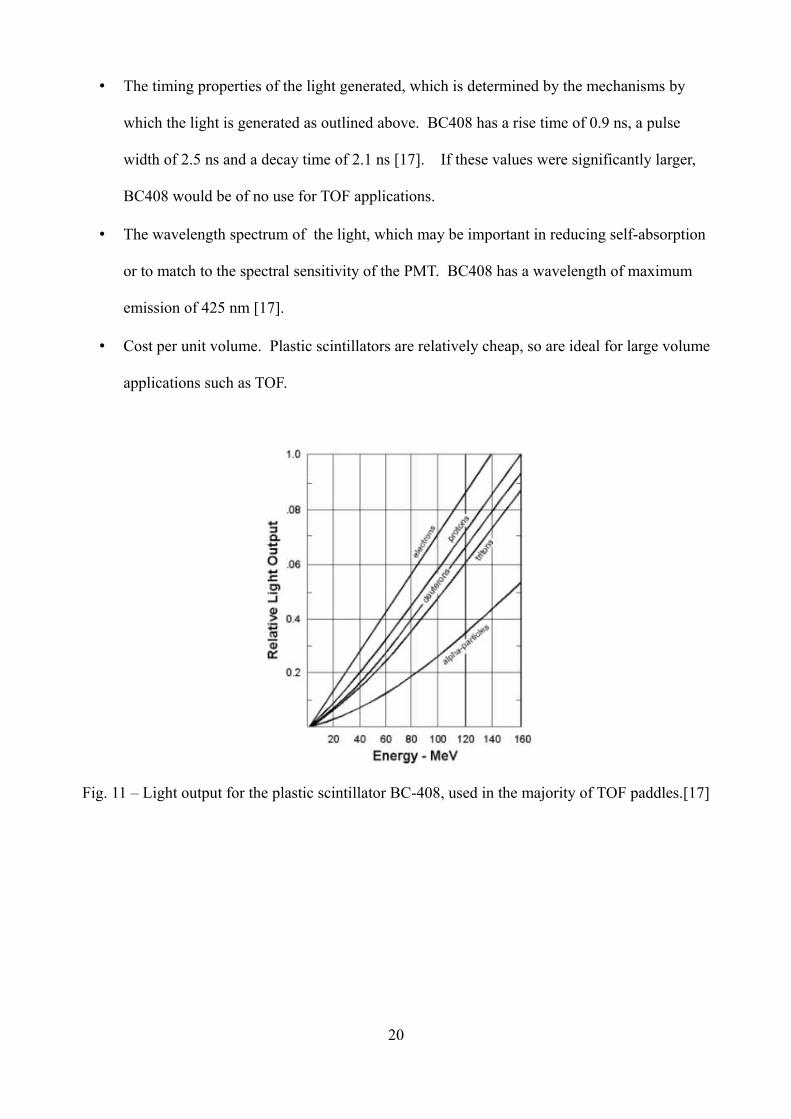
• The amount of light generated by the particle of the type and energy that is to be detected,

see Fig. 11 for the light response of BC408 to a range of particles and energies.

19

• The timing properties of the light generated, which is determined by the mechanisms by

which the light is generated as outlined above. BC408 has a rise time of 0.9 ns, a pulse

width of 2.5 ns and a decay time of 2.1 ns [17]. If these values were significantly larger,

BC408 would be of no use for TOF applications.

• The wavelength spectrum of the light, which may be important in reducing self-absorption

or to match to the spectral sensitivity of the PMT. BC408 has a wavelength of maximum

emission of 425 nm [17].

• Cost per unit volume. Plastic scintillators are relatively cheap, so are ideal for large volume

applications such as TOF.

Fig. 11 – Light output for the plastic scintillator BC-408, used in the majority of TOF paddles.[17]

20

3. Software Background

3. 1 Overview of reconstruction software

The raw data output by the CLAS12 detector is divided into events, where an event is some

suitably small time window (yet to be defined), within which signals generated in the detector

subsystems are potentially related, having been triggered by the same particle. Each event contains

raw data from all the detector subsystems, including FTOF and CTOF. This raw data is not

immediately useful to experimental physicists, who prefer to work with high level concepts such as

the particle ID (PID), four momenta and scattering angles of every particle in an event. This

process of converting between low and high level data is known as reconstruction, and is performed

by the reconstruction software. Note that reconstruction is not performed in real time as the

detector is taking data (online), but rather the output from the detector is stored on tape for later

reconstruction (offline). Part of offline reconstruction is to distinguish between signals left by

particles which have interacted with the target, and background signals caused by another source,

such as cosmic radiation, or beamline particles that did not interact with the target, but still

interacted with the detector.

One of the new features of the CLAS12 offline reconstruction software is that it runs within

the CLARA software framework (CLAS12 Reconstruction and Analysis framework) described in

[10]. As such, it is highly modular in nature, being composed of a linked chain of services -

atomic, self-contained pieces of software, similar in definition and functionality to a SOA (Service

Oriented Architecture) service. For each detector subsystem, their exists (or will shortly exist) a

service whose sole function is to reconstruct the data for that particular subsystem. Each detector

service accepts an input event from the proceeding service in the chain, performs its reconstruction

by running its Execute() function, then forwards its reconstructed data, as well as all existing data,

onto the next service in the chain. Data is sent between services in the Event Input Output format

(EVIO), which is a JLab specific format. At the end of the chain, another service, the Event

21

Builder, combines the data from all the detector subsystems, and outputs the desired high level

parameters, which can be stored and potentially displayed on a GUI.

To illustrate the use of services, a hypothetical chain of services that could be used to

reconstruct the data of the forward detector is shown in Fig. 12. Fig. 12 is not intended to provide a

final representation of the reconstruction application, which is still being developed.

Notice that in Fig. 12 there is a data connection from the end of the chain – the Event

Builder service - back to the beginning of the chain – the LTCC service (refer back to the list of

abbreviations if necessary). This illustrates that reconstruction is not a linear process, but an

iterative one. Reconstruction results for a particular detector service can often be improved using

the reconstructed output from another detector service, hence the need to loop back through the

chain. For example, the DC can fit better particle tracks using the output from the FTOF. On the

first pass through the chain, the DC service calculates particle tracks using hit DC wire positions

only; this is known as hit-based tracking. On the second pass, the precise hit times from the FTOF

service are used to refit the tracks; this is known as time-based tracking. Time-based tracks have

improved resolution. As will be explained in section 3.2, FTOF is also dependent on the DC to

provide hit positions if the FTOF malfunctions.

Fig. 12 also illustrates the use of two special services that sit apart from the main

reconstruction chain: the Geometry service, which provides constants that describe the position,

size and orientation of detector components, and the Calibration service, which provides constants

needed to convert raw detector data into physical quantities such as time and energy. Detector

services request data from the geometry and calibration services as and when needed, typically

when processing a new data set taken with a new detector set-up. Data is returned in the form of an

XML file.

The services of Fig. 12 only deal with the processing of physics data; specialist computing

issues, such as parallel and distributed computing are dealt with by the CLARA platform itself.

22

This allows physicists who are not computer experts to write services. Further, to allow the widest

possible group of people to contribute to the CLAS12 project, services can be written in one of

several high level programming languages including Java, which was used for this project. In Java,

writing a service simply means implementing the interface of a specific class. As the author of a

Java service, it does not matter how any other service is implemented, or even what language is

used, only a common input/output format is important.

In the context of the overall reconstruction application, the CTOF and FTOF reconstruction

services perform identical functions for the central and forward detectors, respectively. They both

convert a list of raw CTOF/FTOF data (ADC/TDC values) into a list of particle hits on the

Fig. 12 - Hypothetical reconstruction application for the forward detector, built from a chain of CLARA services.

23

CTOF/FTOF. These hits have properties of position, time and energy deposited. The next step in

the reconstruction process, which would be carried out by the Event Builder service in Fig. 12, is to

match these hits with particle tracks generated by the DC service, for the forward detector, and by

the SVT/BMT services, for the central detector. Once the hits are matched to tracks, the velocity of

a particle can be calculated using the path length of the track from the target to the TOF hit position

divided by the TOF hit time (velocity = distance/time). Dividing the momentum of the track by

the velocity gives relativistic mass (relativistic mass = momentum/velocity), which, when combined

with data from other detectors such as the LTCC and HTCC, helps identify the particle. In

practice, the identification of particles is not a black and white process, rather it involves the

calculation of probabilities that a track is due to a specific type of particle. The most likely

candidate is the one the Event Builder would output.

3.2 CLAS6 FTOF Reconstruction Software

The CLAS12 FTOF and CTOF reconstruction services are based on the FTOF code in the

existing CLAS6 reconstruction software written in C and Fortran. The behaviour of the CLAS6

code is documented in the code itself, and to some extent in [7] and [8]. It can be summarized as

follows:

• Step 1: Read in calibration and geometry variables

Constants appropriate to the data run, identified by the run number, are read in from the

calibration and geometry databases.

• Step 2: Convert raw ADC and TDC signals to energy and time, respectively

The input for each hit paddle consists of a paddle ID, which uniquely identifies the paddle,

and left and right ADC and TDC values. The raw ADC values are converted into energy deposited

in MeV using

Edep=ADC−PEDESTAL⋅DEDX NMIP⋅THICKNESS /ADC NMIP (1)

24

where ADC is the raw ADC value in channels, PEDESTAL is the ADC value in channels when no

data is present, DEDXNMIP is the energy loss per unit length in MeV/cm for a NMIP (Normally

Incident Mimimum Ionizing particle), THICKNESS is the thickness of the paddle in cm and

ADCNMIP is the pedestal-subtracted ADC value in channels corresponding to a 10 MeV NMIP. The

raw TDC values are converted into times in ns using

T TOF=PULSER⋅(T0+ T1⋅TDC+ T2⋅TDC 2+ TIMEWALK ) (2)

where PULSER is the pulser normalization constant, TDC in the raw TDC value in channels, T0,

T1 and T2 are fitting constants and TIMEWALK is defined using

TIMEWALK=f w(ADCREF /DISCTHRESH )−f w((ADC−PEDESTAL)/DISCTHRESH) (3)

where ADCREF is the reference ADC value in channels, DISCTHRESH is the ADC discriminator

threshold in channels and fw(X) is defined using

f w (X )=WALK1 /XWALK2 (4)

if X < WALK0, and

f w(X )=WALK1⋅(1.0+ WALK2) /WALK0WALK2−WALK1⋅WALK2⋅X /WALK0WALK2+ 1.0 (5)

if X > WALK0, where WALK0, WALK1 and WALK2 are fitting constants. Uncertainties in time

and energy are also calculated.

• Step 3: Combine left and right times and energies

A status integer is associated with each paddle, indicating the completeness of that paddle's

data, see App. A. Depending on the status integer of the paddle, the data from the left and right

PMTs is combined using different equations. If both left and right ADC and TDCs have valid

readings, then the hit sector y position (see Fig. 7) in cm is calculated using

Y=VEFF L⋅VEFF R⋅(TIMEL−TIMER−YOFFSET ) /(VEFFL+ VEFF R) (6)

where VEFFR and VEFFL are the effective velocities of right and left moving light respectively, and

YOFFSET is a constant. The coordinate system was defined in Fig. 7. If only one TDC time is

known, an attempt is made to use a tracking input calculated using external detector subsystems, to

25

calculate the y position. If this fails, but both ADC energies are known, the y position is calculated

instead using

Y =ATTEN L⋅ATTEN R⋅log(ENERGY L/ENERGY R)/(ATTEN L+ ATTEN R) (7)

where ATTENL and ATTENR are the attenuation lengths for left and right moving light

respectively. The attenuation length is defined as the distance at which the intensity of a beam of

particles has dropped to 1/e of its original value. Note that the x and z positions are always assumed

to be on the centre line of the paddle, as there is no way of knowing otherwise. Once the y position

is known, and both TDC times are known, the hit time can be calculated using

T TOF=(TIME L+ TIME R)/2.0−Y⋅(VEFF R−VEFF L)/ (2.0⋅VEFF R⋅VEFF L) (8)

If only one TDC time is known, the hit time is calculated using

T TOF=TIME L−Y /VEFF R−YOFFSET /2 (9)

or

T TOF=TIME R+ Y /VEFF L+ YOFFSET /2 (10)

depending on which TDC is missing. If both ADC energies are known, the hit energy deposited is

calculated using

Edep=√ENERGY L⋅ENERGY R⋅exp(Y⋅(ATTEN R−ATTEN L)/(ATTEN L⋅ATTEN R)) (11)

or if only one ADC energy is known, the hit energy is calculated using

Edep=ENERGY L⋅exp (Y / ATTEN L) (12)

or

Edep=ENERGY R⋅exp(Y /ATTEN R) (13)

depending on which TDC is missing. Uncertainties in hit time, energy and position are also

calculated.

• Step 4: Group adjacent related paddle hits into clusters

To deal with the fact that a single particle can leave signals in multiple adjacent paddles, due

to an initial trajectory that passes through multiple paddles, or to scattering within the paddles, the

26

final step in the reconstruction is to combine related hits into clusters. A cluster has the summed

energy of all its composing hits. This step is described in detail in section 5.3.2, as a modified

version of this step is one of the key differences between the CLAS12 and CLAS6 TOF algorithms

• Step 5: Output

The output from steps 2, 3 and 4 is stored in permanent data banks. The software is also

capable of reading back in the output banks and redoing steps 3 and 4 using time-based, rather than

hit-based, tracking (introduced in section 3.2) to give more accurate hit locations and therefore more

accurate hit times.

3.3 Simulation of the CLAS12 Detector: DISGEN and GEMC

The CLAS12 detector is still in the process of being built, so it was not possible to design or

test the reconstruction services using data from the CLAS12 detector. Instead, simulation was used

to create data which resembled, in as much as is possible, the type of data CLAS12 will be

generating when it comes online. The process by which this data was created is summarized below:

DISGEN → GEMC → CTOF / FTOF service

(event generator) (simulates CLAS12 detector)

Particles consistent with the deep inelastic scattering of electrons from a Hydrogen target are

created by a program called the Deep Inelastic Scattering generator, or DISGEN. For the DISGEN

parameters used, see App. L. The output of DISGEN is fed into a program called GEMC, or

GEANT 4 Monte Carlo, which models the geometry and response of the CLAS12 detector and

optionally adds in background hits due to the presence of the beam. For the GEMC parameters

used, see App. M. See also Fig. 13 for an example particle interaction in the GEMC simulation of

the CLAS12 detector. The output from GEMC is fed into the CTOF or FTOF service. This output,

27

detailed in appendices E and J, for FTOF and CTOF respectively, contains not only the ADC and

TDC values the real detector would output, but also other fields, such as the original energies and

times from which these digitizations were derived, plus 3D hit position, momentum of particles at

the TOF paddles and PID. These additional fields are unique to GEMC, and would not be known in

the real detector. As the ADC and TDC values output by GEMC do not use the calibration

Equations 1-13 of section 3.2, the FTOF and CTOF services have an option to not use Equations 1-

13 at all, but rather to digitize the energy and time themselves (using reversed versions of Equations

1-13 of section 3.2), and use these digitizations as their input, see section 5.1. GEMC simulation

results for CTOF and FTOF are given in section 4.

Fig. 13 – Annotated output from the GUI of the CLAS12 simulation software GEMC. Two simulated tracks produced hits (in red) in the various detectors. Photons are the blue straight tracks.[12]

28

4. Simulation Results

This section contains a subset of the results obtained from simulations of the CLAS12

detector using DISGEN, GEMC, and analysed with the TOF reconstruction software, as explained

in section 3.3. Results are intentionally explained very briefly. Unless otherwise indicated, the

beam consists of 11 GeV electrons, and GEMC adds in background due to the presence of the

beam. Note that the detector geometry on which these simulations are based is an early revision

and is not identical to the final detector geometry.

4.1 CTOF

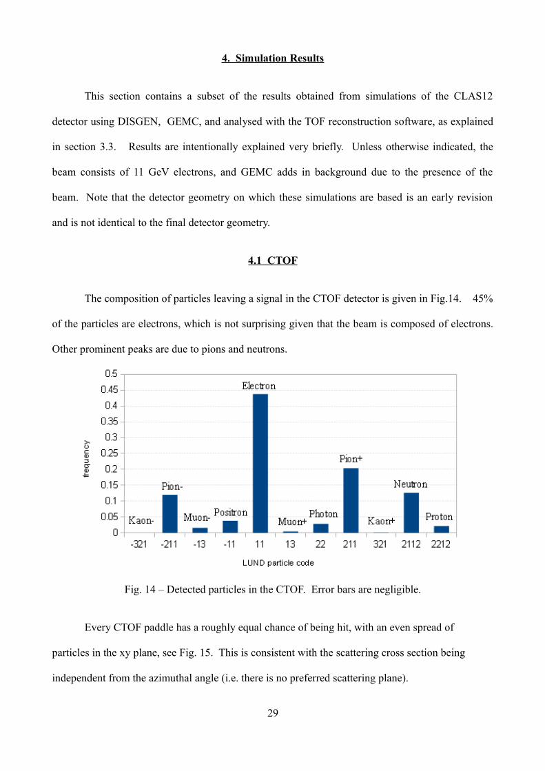
The composition of particles leaving a signal in the CTOF detector is given in Fig.14. 45%

of the particles are electrons, which is not surprising given that the beam is composed of electrons.

Other prominent peaks are due to pions and neutrons.

Fig. 14 – Detected particles in the CTOF. Error bars are negligible.

Every CTOF paddle has a roughly equal chance of being hit, with an even spread of

particles in the xy plane, see Fig. 15. This is consistent with the scattering cross section being

independent from the azimuthal angle (i.e. there is no preferred scattering plane).

29

PhotonK+

Fig. 15 – CTOF particle hit location in xy plane. Signal and background.

Fig. 16 – CTOF particle hit location in xy plane. Background only

30

-40 -30 -20 -10 0 10 20 30 40

-40

-30

-20

-10

0

10

20

30

40

x position, CLAS coordinates (cm)

y po

sitio

n, C

LAS

coo

rdin

ates

(cm

)

-40 -30 -20 -10 0 10 20 30 40

-40

-30

-20

-10

0

10

20

30

40

x position, CLAS coordinates (cm)

y po

sitio

n, C

LAS

coo

rdin

ates

(cm

)

Hits due to the background are also roughly evenly distributed in the xy plane, see Fig. 16,

with background hits only contributing about 3% to the total number of hits.

Fig. 17 shows the distribution of GEMC energy deposited at the CTOF paddles. This is the

simulated energy that a particle deposits on its journey through the simulated paddle. Note the

logarithmic frequency scale. Many of the particles deposit less than 1 MeV. Many hits depositing

low amounts of energy will be removed by the ADC discriminator, which had a threshold of

approximately 0.7 MeV in CLAS6, but is yet to be set for CLAS12. Above 1 MeV, there is an

exponential drop off in frequency, due to an increasing rarity of particles able to deposit a given

amount of energy. The particles that can deposit the most energy are typically heavier, for example

pions and protons, and have an entrance energy of 0.5-11 GeV. An exception to the general pattern

is the peak at around 10 MeV, which is due to Minimum Ionizing Particles (MIP).

Fig. 17 – GEMC energy deposited of CTOF hits.

Fig. 18 shows the distribution of GEMC time. This is the time between the interaction at

the target, and the hit in a CTOF paddle. The earliest particles arrive after about 1 ns. There is a

peak in frequency at about 1.2 ns, due to particles with the most common flight path and velocity,

31

which will be mostly electrons. At higher times, there is an exponential drop off in frequency, due

to the increasing rarity of some combination of lower velocity (due to higher mass, for example)

and longer flight path.

Fig. 18– GEMC time of CTOF hits.

4.2 FTOF

Fig. 19, equivalent to Fig. 14 for CTOF, shows the particle ID of detected particles at Panel-

1b of the FTOF detector. Over 50% of detected particles are electrons, with other prominent

peaks due to pions, positrons and protons.

Fig. 20 shows how often a signal is left at each of the panel types – 1a,1b and 2. The

structure of the panels was described in section 2.2, recall Fig. 9. Panel-1b receives a greater

proportion of hits than panel-1a. This is for three main reasons: (1) panel-1b covers a slightly

larger area than panel-1a, (2) panel-1b is located in front of panel-1a, so it shields panel-1a from

low energy, secondary particles created by the primary particles travelling through panel-1b and (3)

panel-1b is more finely segmented than panel-1a, so it can separate output multiple signals due to

physically close particles, whereas panel-1a cannot distinguish between two particles that hit the

same paddle. Panel 2 has a lower hit frequency as it has fewer paddles and is located at wider

32

angles.

Fig.19 – Detected particles at Panel-1b. Error bars are negligible.

Fig. 20 – Proportion of total hits which strike a particular panel type. Error bars are negligible.

Fig. 21 shows the locations of hits on panels 1b and 2 in the xy plane. Hits are concentrated

in the central region of the detector, due in part to the background hits which are shown separately

in Fig. 22. Fig 22. shows that panel-1b shields panel-1a quite significantly from the background,

and that panel-2 receives very few background hits due to its distance from the beam. As a rough

estimate, 1% of panel-1a, 6% of panel-1b, and 0.1% of panel-2 hits, are due to background hits.

33

Fig. 21 – Hit locations in xy plane for signal plus background on panels 1b and 2.

Fig. 22 – Hit locations in xy plane for background only on panels 1a, 1b and 2.

34

Fig. 23, equivalent to Fig. 17 for CTOF, shows the GEMC energy deposited for all panel

types. This graph looks almost identical with and without background and with 11 or 6 GeV beam

energies. Like CTOF, most particles deposit very little energy, with an exponential drop off in

frequency with increasing energy. Like CTOF, each panel has a peak due to MIPs. Panel-1a (blue

histogram) and panel-2 (yellow histogram) have paddles of the same thickness (5cm), hence they

both have a peak due to MIPs at the same place, approximately 10 MeV. Panel-1a (red histogram)

has thicker paddles (6cm), hence a MIP can deposit more energy, approximately 12 MeV. The ratio

of peak energies is identical to the ratio of thicknesses.

Fig. 23 – GEMC energy deposited for all three panel types, events and background

Fig. 24 shows the GEMC energy deposited for the background only. It decays more quickly

with energy, cutting off at about 14 MeV.

Fig. 25, equivalent to Fig. 18 for CTOF, shows the GEMC time for all panel types. As with

CTOF, there is a minimum time due to particles having to travel from the target to the FTOF panels

roughly 6.5 metres away. Geometry also explains the three peaks, one for each panel, with the

35

Fig. 24 – GEMC energy deposited by background only for panel 1b (similar for all panels)

ordering of the peaks determined by their distance from the target, particles obviously hitting closer

things sooner. The 0.4 ns time difference between the peaks for panel-1a and 1b is consistent with

the inter-panel distance, which is about 11cm. As for CTOF, the spread in the peaks is due to the

spread in velocity and path length.

Fig. 25 – GEMC time for all three panel types.

36

5. CLAS12 FTOF Reconstruction Service

5.1 Overview

The CLAS12 FTOF reconstruction service performs the same function as the CLAS6 FTOF

reconstruction software described in section 3.2, namely to convert ADC and TDC readings into the

energy, time and position of particle hits and clusters (groups of hits) on the FTOF panels. Where

appropriate, algorithms and equations have been directly re-used from CLAS6. The main

differences between the CLAS6 and CLAS12 applications are:

1. The programming language – CLAS6 used C, CLAS12 uses Java.

2. The software framework - CLAS12 uses the CLARA framework, new to the CLAS12 era.

3. The format of the input/output data – CLAS12 uses EVIO, new to the CLAS12 era.

4. The structure of the geometry – CLAS12 and CLAS6 have a different panel structure.

5. The implementation of the clustering algorithm – as discussed in section 5.3, the CLAS6

clustering algorithm has been altered for CLAS12 so as to make it more efficient and

configurable.

The main input to the FTOF service is a transient file in EVIO format, which, for each event

in the detector, consists of banks (columns) of data containing the output from the real or simulated

detector. Although the EVIO may contain banks from all detector subsystems, the banks relevant to

the FTOF service consist of three sets of banks, one for each panel type – 1a, 1b and 2. These

banks contain the left and right ADC and TDC values from any triggered paddles in an event. The

format of these input banks is specified in App. B.

The FTOF service has two additional inputs, which are used to set-up the service prior to

execution of the main reconstruction algorithm. The detector geometry for a particular data run is

retrieved from the geometry service in the form of an xml file. The format of this is specified in

App. C. Currently, the service attempts to retrieve the xml from the geometry service, but if this

fails, it uses default values. The detector calibration for a particular data run will be retrieved from

37

the calibration service, when it exists. Currently default values are used. The proposed format of

this is specified in App. D.

The output from the service is an identical EVIO file to the input, but with the addition of

three new sets of banks. These are outlined here, see App. E for the full definitions. The Converted

Raw banks contain, for each paddle hit in an event, the left and right ADC and TDC values

converted to energy and time, respectively. The Hit banks contain, for each paddle hit in an event,

the time, energy and position of that hit, thus combining the left and right PMT data. The Cluster

banks contain, for each cluster of related adjacent hits in an event, the time, energy and position of

that cluster. These banks are very similar to the CLAS6 banks. Note that if the reconstruction

service cannot process the input EVIO for whatever reason, the input EVIO is returned unchanged,

other than with the addition of a message indicating the error.

The input and output from the FTOF reconstruction service is summarized in Fig. 26.

Fig. 26 – The inputs and outputs of the FTOF reconstruction service

Turning to the specifics of the service implementation, functionality lives in one of two

functions of the FTOF service class.

38

The Configure() function is used to set-up the service. The workflow of the Configure()

function is shown in Fig. 27. It reads in the calibration and geometry constants and, if options are

supplied as an argument, will configure the service as specified. A list of service options can be

found in App. F. The most important option is the “input-data” option, which alters how the

service processes the input bank depending on whether it contains real or simulated data. This is

explained in Fig. 28. Although GEMC outputs TDC and ADC values, they are calculated using

dummy equations, not using the full set of calibration equations and variables described in section

3.2. The “input-data” option exists to obtain more realistic TDC and ADC values. Another

important option, for test purposes, is the “processExactGEMCvalues” option which when set to

“true” means that the service will, in parallel with the input ADC/TDC values, or reversed

ADC/TDC values, pass the exact GEMC time energy and position through the reconstruction. This

allows comparisons to be made between simulated and reconstructed data.

Fig. 27 – The FTOF reconstruction service Configure() function. This function is used to set up the geometry and calibration constants of the service and to select service options.

39

Fig. 28 – FTOF service workflow differences due to the “input-data” configuration option.

40

Unlike the Configure() function, which is run as and when needed, the Execute() function is

run automatically for every event. It carries out the main processing of the service by reading in

the input EVIO, reconstructing the data contained therein, then adding the results to the EVIO.

Fig. 29 summarizes the operation of the Execute() function.

Fig. 29 – The FTOF reconstruction execute() function. Run once for every input event.

41

The Java classes that implement the FTOF service are divided into seven packages, see

Table 1. These packages are explained in greater detail in the following sections, where necessary.

Package Contents

Calibration Classes to import and store calibration data from the calibration service, or

hard-coded defaults

Geometry Classes to import and store geometry data from the geometry service, or

hard-coded defaults

Event Classes to store detector data associated with a single event

Reconstruction Classes that implement the reconstruction algorithm by manipulating the data

stored in the Event classes

Services The CLARA service class which enables the code to be integrated as a service

in the CLARA environment. The Configure() and Execute() functions are

implemented here.

Detector Classes to store miscellaneous constants, including the numbers that identify

the EVIO banks

Standalone Class to run the service on the local machine without using the CLARA

platform

Table 1 – outline of the FTOF reconstruction service packages.

42

5. 2 Details of Software Packages

5.2.1 Calibration

The calibration package contains classes to import and store calibration parameters. These

parameters are currently hardcoded, but will eventually be supplied by the calibration service. Code

has already been written to read in the proposed calibration service XML, specified in App. D.

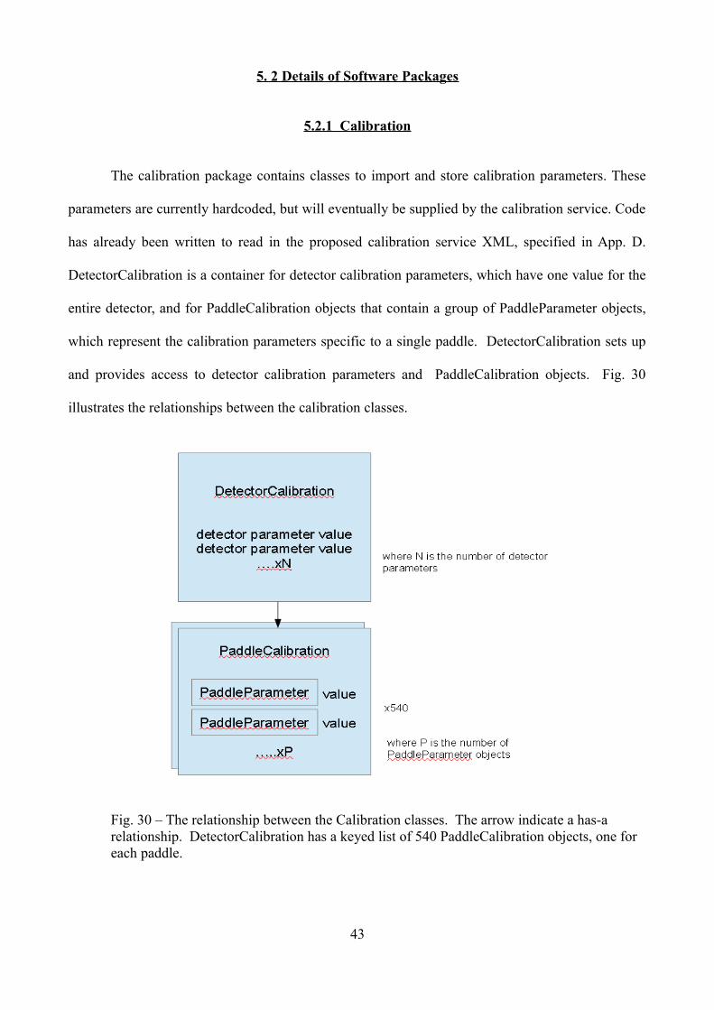
DetectorCalibration is a container for detector calibration parameters, which have one value for the

entire detector, and for PaddleCalibration objects that contain a group of PaddleParameter objects,

which represent the calibration parameters specific to a single paddle. DetectorCalibration sets up

and provides access to detector calibration parameters and PaddleCalibration objects. Fig. 30

illustrates the relationships between the calibration classes.

Fig. 30 – The relationship between the Calibration classes. The arrow indicate a has-a relationship. DetectorCalibration has a keyed list of 540 PaddleCalibration objects, one for each paddle.

43

5.2.2 Geometry

The geometry package contains classes to import and store geometry data supplied by the

geometry service. The geometry service XML can be found in App. C. The hierarchy is

DetectorGeometry->PanelGeometry->PaddleGeometry. PaddleGeometry stores data unique to a

paddle (e.g. paddle centre position), PanelGeometry stores data unique to a panel (e.g. thickness of

all paddles on a panel), and DetectorGeometry is used to create and access PanelGeometry objects.

Fig. 31 illustrates the relationships between the geometry classes.

Fig. 31 – Relationship between the Geometry classes. An arrow indicates the has-a relationship. There are 18 PanelGeometry objects as each of the six sectors has a panel-1a, 1b and 2.

5.2.3 Event

The event package contains classes to store reconstruction data relating to a single event, see

Fig 32 for the relationships between these classes. EventData is a container for the data from the

entire event, likewise SectorData for the sector and PanelData for the panel. Each PanelData object

has associated with it Paddle and Cluster objects. A Paddle represents a physical TOF paddle. It

primarily stores the ADC and TDC values from the PMT attached to either end of the paddle, plus

the energy and time theses values correspond to. Each Paddle has a Hit object associated with it

that represents the combined data from the left and right PMTs of a paddle. It primarily stores the

44

time, energy and position of the hit. A Cluster represents the combined data from N adjacent hits

on a panel. It primarily stores the time, energy and position of the cluster. If the service is running

in ProcessExactGEMCValues mode, then each Paddle object also has a GEMCHit, and each

PanelData one or more GEMCClusters. A GEMCHit primarily stores the GEMC time and energy

and position supplied in the input EVIO. It also stores GEMC specific fields, such as the particle

ID, entrance energy and particle momentum at the paddle. A GEMCCluster represents the

combined data from N adjacent GEMCHits, where the makeup of the clusters is copied over from

the Cluster object. The existence of these GEMC objects allows for a direct comparison to be made

between simulated and reconstructed data.

Fig. 32 – The Event package classes. The arrows represent the has-a relationship. GEMCHit and GEMCCluster only exist if processExactGEMCValues is set to true.

5.2.4 Reconstruction

5.2.4.1 Overview

The reconstruction package contains classes that implement the reconstruction algorithm by

manipulating the data stored in the Event package classes. The function of each class is

45

summarized in Table 2.

Function Class name

Creates an alternative input to the reconstruction byreversing from GEMC time, energy and position back to ADC and TDC values. ReverseEngineer

Creates Paddle and (optionally) GEMCHit objects from the input EVIO. PaddleReader

If necessary, adjusts raw ADC/TDC values due to hardware faults and miscabling PaddleCorrector

Coverts raw ADC/TDC values into times and energies. PaddleConvertor

Reconstructs a single paddle by creating and addinga Hit object to each Paddle. PaddleReconstruction

Reconstruct a single panel by creating one or more Cluster objects from adjacent related Hit objects andadding them to the PanelData. (Optionally) createsGEMCCluster objects from Cluster objects. PanelReconstruction

Reconstructs a single sector usingPanelReconstruction and PaddleReconstruction. SectorReconstruction

Finds optimal clustering parameters and clusteringefficiency of a given clustering configuration ConfigPanelReconstructionCLAS12

Creates an output EVIO bank for each Paddle, Hit and Cluster object i.e. Converted Raw,Hit and Cluster banks, respectively OutputCreator

Table 2 – Summary of the reconstruction package classes.

5.2.4.2 ReverseEngineer Class

The ReverseEngineer class implements inverted versions of the equations found in

PaddleReader and PaddleReconstruction and described in section 3.2, for the case that a paddle

has valid readings from both left and right side ADCs and TDCs. It takes as input GEMC time,

energy and position and outputs left and right ADC and TDC values. This class is necessary as the

ADC and TDC values that GEMC outputs are not calculated using the calibration equations

46

described in section 3.2. It is only ever used with the service option “input-data” is set to

“simulated”.

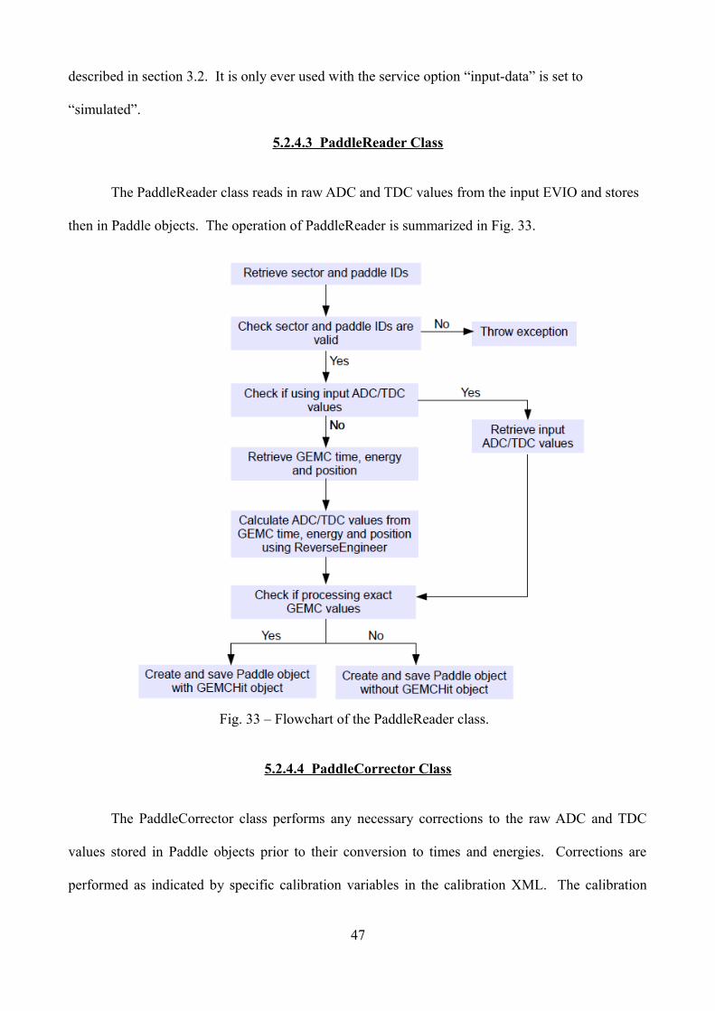
5.2.4.3 PaddleReader Class

The PaddleReader class reads in raw ADC and TDC values from the input EVIO and stores

then in Paddle objects. The operation of PaddleReader is summarized in Fig. 33.

Fig. 33 – Flowchart of the PaddleReader class.

5.2.4.4 PaddleCorrector Class

The PaddleCorrector class performs any necessary corrections to the raw ADC and TDC

values stored in Paddle objects prior to their conversion to times and energies. Corrections are

performed as indicated by specific calibration variables in the calibration XML. The calibration

47

variable “status” is set to 0,1,2 or 3 for each PMT, see Table 3. If the status variable indicates an

missing ADC/TDC, the output of this ADC/TDC is zeroed.

value of “status” variable meaning

0 both TDC and ADC working fine

1 no ADC

2 no TDC

3 no ADC or TDC

Table 3 – Definition of the “status” calibration variable.

The calibration variables “swapADC” and “swapTDC” are used to swap the values of

paddles due to miscabling. Each paddle is given a calibration index from 1 to 540, proceeding

logically from sector 1 to 6, and in each sector proceeding from panel-1a to 1b to 2, and within each

panel proceeding from the lowest to the highest paddle ID. If two paddles have had their cables

switched over for a TDC, for example, then the value of swapTDC for paddle one is set to the index

of paddle two, and vice versa. In the software, the raw TDC values will be switched over before

conversion to time. The same applies to ADC values for swapADC.

The operation of PaddleCorrector is summarized in Fig. 34.

Fig. 34 – Flowchart of the PaddleCorrector class

48

5.2.4.5 PaddleConvertor Class

The PaddleConvertor class converts raw ADC/TDC values into energies and times. The

operation of PaddleConvertor is summarized in Fig. 35. The conversions of TDC to time and ADC

to energy are currently performed using the same calibration equations as those in CLAS6, see

section 3.2, step 2.

Fig. 35 – Flowchart of the PaddleConvertor class

5.2.4.6 SectorReconstruction Class

SectorReconstruction reconstructs one sector of the detector. SectorReconstruction simply

loops over all PanelData objects in a SectorData object, using PanelReconstruction to reconstruct all

panels in a sector.

5.2.4.7 PanelReconstructionCLAS12 class

PanelReconstruction reconstructs one panel of the detector. It uses PaddleReconstruction to

reconstruct each Paddle, then creates one or more Cluster objects from adjacent related Hit objects

and adds them to the PanelData. See section 5.3 for more details.

49

5.2.4.8 ConfigPanelReconstructionCLAS12 Class

ConfigPanelReconstructionCLAS12 outputs to file information that can be used to

determine the clustering efficiency and the optimal clustering parameters of the CLAS12 clustering

algorithm, see section 5.3 for the theory, and [16] for the practical details of how to use the class.

5.2.4.9 PaddleReconstruction Class

PaddleReconstruction reconstructs one paddle of the detector, by creating and adding

a Hit object to each Paddle. The calculation of the Hit properties from the left and right times and

energies is currently done using the CLAS6 calibration equations described in section 3.2, step 3.

Like CLAS6, it uses the status integer specified in App. A to decide which of the equations to use

for each Paddle. Currently, the tracking input has not been implemented.

5.2.4.10 OutputCreator Class

OutputCreator populates the banks of the output EVIO. Values for the fields of the

Converted Raw, Hit and Cluster banks, defined in App. E, are read from Paddle, Hit and Cluster

objects, respectively.

50

5.3 Clustering Algorithm for CLAS12

5.3.1 Overview

Because it is possible for a single incoming particle to trigger multiple FTOF paddles, the

CLAS6 FTOF reconstruction software includes code that searches for related adjacent paddle hits,

then combines them into clusters. This section describes this process, then explains, using the

results from GEMC simulations, how it could be altered for CLAS12. These alterations have been

implemented in the configurable class PanelReconstructionCLAS12, described in full in section

5.3.8.

5.3.2 Description of the CLAS6 Algorithm

There is an alternative description of the CLAS6 clustering algorithm in [7]. The

description given here is broken down into questions and answers to highlight the essential features.

Alternative answers to these questions suggest possible ways of changing the algorithm.

(1) How are two adjacent paddle hits considered related and hence worthy of clustering?

Two adjacent paddle hits are considered related if the absolute difference in sector y

positions (∆y) is less than 3 times the combined uncertainty in sector y positions, or, in

symbols,

y3∗ y12 y2

2 , (14)

where δy1 and δy2 are the uncertainties in the hit 1 and hit 2 sector y positions, respectively,

calculated using standard error equation equivalents of the relevant equations in section 3.2

(the error equations are complicated and for space considerations are not included in this

thesis, see the code itself)

AND the absolute difference in times (∆t) is less than 3 times the combined uncertainty in

times, or, in symbols,

t3∗t12t2

2 , (15)

51

where δt1 and δt2 are the uncertainties in the hit 1 and hit 2 times, respectively, again

calculated using standard error equations. The factor of 3 on the right side of these

equations is used for all panels.

(2) What is the maximum number of adjacent paddle hits from which a cluster is created?

Two. Non-adjacent hits, or non-related hits become single hit clusters.

(3) If there are more adjacent paddle hits than the maximum cluster size, which of the hits are

combined?

If there are three or more adjacent related paddle hits, the algorithm will only combine two

of them, the other hits becoming single hit clusters. The first pair (with lowest paddle IDs,

closest to beam line) will be combined into a cluster if (1) the combined time uncertainty for

the second pair is greater than the combined time uncertainty for the first pair, OR (2) the

combined y uncertainty for the second pair is greater than the combined y uncertainty for the

first pair , OR (3) the second pair fails the test previously defined for deciding if adjacent

paddle hits are related.

(4) How are the individual parameters of the hits combined when creating a cluster?

For double hit clusters: The cluster energy is the sum of the hit energies. The cluster time is

the energy-weighted average of the hit times. The cluster y position is the energy-weighted

average of the hit y positions. The x and z positions are simple averages of the hit x and z

positions, which lie on the centre line of the paddle. The cluster paddle ID is the paddle ID

of the first hit. The cluster status is the status of the first hit plus 100 times the status of the

second hit.

For single hit clusters: the cluster parameters are copied over unchanged from the hit.

52

5.3.3 GEMC Clustering Reference

5.3.3.1 Concept

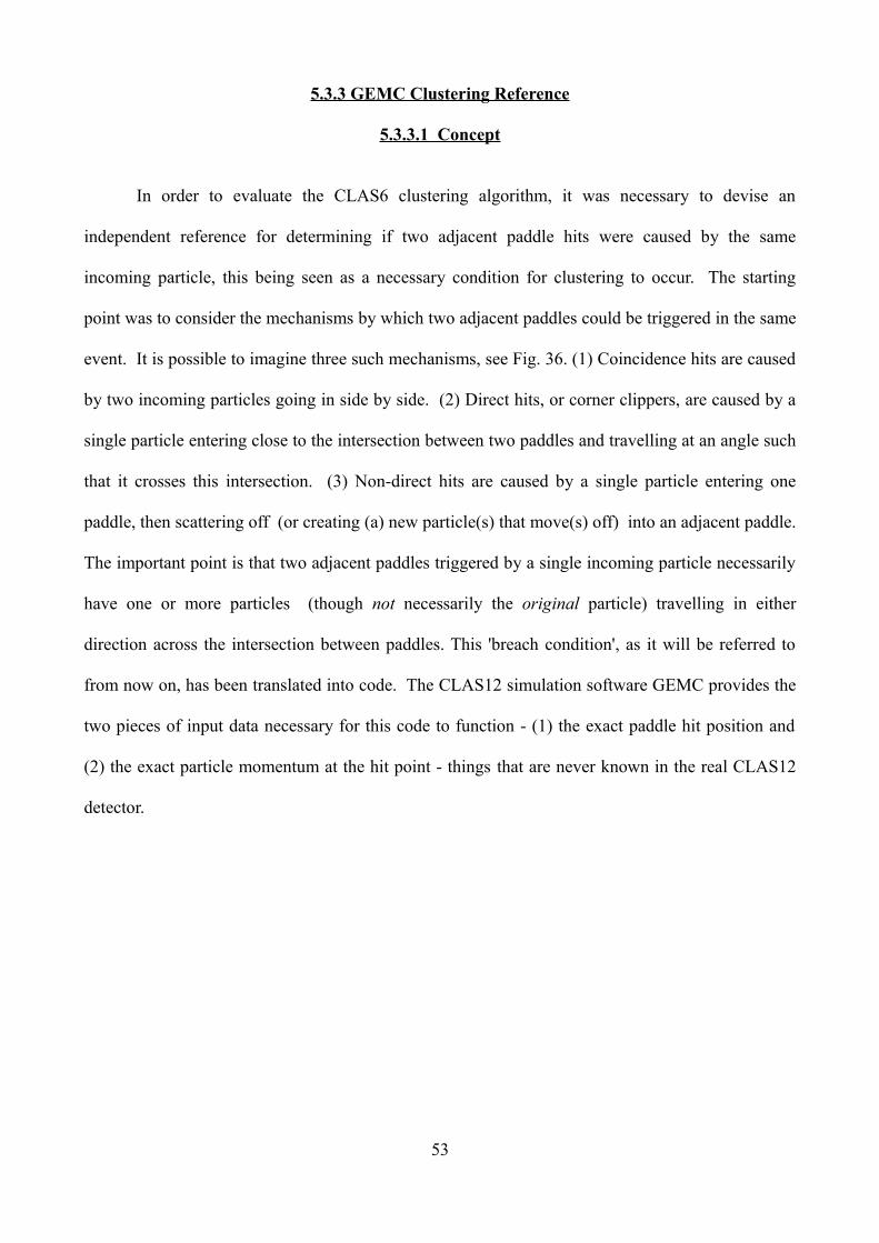
In order to evaluate the CLAS6 clustering algorithm, it was necessary to devise an

independent reference for determining if two adjacent paddle hits were caused by the same

incoming particle, this being seen as a necessary condition for clustering to occur. The starting

point was to consider the mechanisms by which two adjacent paddles could be triggered in the same

event. It is possible to imagine three such mechanisms, see Fig. 36. (1) Coincidence hits are caused

by two incoming particles going in side by side. (2) Direct hits, or corner clippers, are caused by a

single particle entering close to the intersection between two paddles and travelling at an angle such

that it crosses this intersection. (3) Non-direct hits are caused by a single particle entering one

paddle, then scattering off (or creating (a) new particle(s) that move(s) off) into an adjacent paddle.

The important point is that two adjacent paddles triggered by a single incoming particle necessarily

have one or more particles (though not necessarily the original particle) travelling in either

direction across the intersection between paddles. This 'breach condition', as it will be referred to

from now on, has been translated into code. The CLAS12 simulation software GEMC provides the

two pieces of input data necessary for this code to function - (1) the exact paddle hit position and

(2) the exact particle momentum at the hit point - things that are never known in the real CLAS12

detector.

53

Fig. 36 – Three ways in which two adjacent paddles can be triggered. This view is in sector 1, in the xz plane, looking down y. The arrows represent the movement of particles.

5.3.3.2 Coding the Breach Condition

The breach condition is shown graphically in Fig. 37. In words, the code that implements

the breach condition can be broken down into the following steps:

1. Using sector coordinates, a line is drawn in the xz plane that bisects the two adjacent

triggered paddles.

2. For one of the paddles, a second line is drawn through the GEMC particle hit position

with the direction of the line determined by the x and z components of the GEMC

momentum. This line therefore approximates the particle's path through the paddle.

3. The intersection point between the two lines found in steps 1 and 2 is calculated.

4. If the intersection point lies within the thickness of the panel, the breach condition is

met. If the intersection lies outside the panel, then the breach condition fails.

5. Steps 2 through 4 are repeated for the other paddle. If either paddle meets the breach

condition, then the code returns that the breach condition has been met for the pair.

Note that it is unnecessary to look for the intersection between the plane between two

54

adjacent paddles and the 3D line approximating the particle's path, rather than the 2D equivalent

described here. This is because the y dimension has been implicitly taken into account by the fact

that both paddles have triggered.

(a) Breach condition is met. The intersection of the line bisecting the paddles and the line through the hit position in the direction of the particle momentum is inside the volume of the paddle.

(b) Breach condition fails. The intersection of the line bisecting the paddles and the line through the hit position in the direction of the particle momentum is outside the volume of the paddle.

Fig. 37 – Graphical illustration of the GEMC breach condition.

55

5.3.3.3 GEMC Clustering Reference Tests

To test the GEMC clustering reference, a sample of data consisting of approximately

200,000 events was created using the procedure outlined in section 3.4. The DISGEN beam energy

was initially set to 11 GeV. Tests performed on this data included the following:

(1) Number of paddles, N, triggered by a single incoming particle (11 GeV electron beam)

By using the GEMC breach condition described in section 5.3.3.2 between all adjacent

paddle hit pairs, it is possible to estimate the frequency with which a single incoming particle

triggers N paddles. For example, if there are 3 adjacent paddles numbered 1 to 3, and, in a given

event, if all these paddles trigger, and paddles 1 and 2, but not 2 and 3, meet the breach condition,

then one incoming particle is assumed to have triggered the first 2 paddles, another particle the

third. This was done separately for each panel type – 1a, 1b and 2. In all cases, particles below 0.7

MeV were ignored, as this is roughly the value of the CLAS6 ADC discriminator threshold.

Results for panel 1a and 1b are shown in Fig. 38. Note that, because panel 2 receives far

fewer hits, and the comparison between panel 1a and 1b is particularly enlightening, panel 2 is not

included in this section.

At small N, panels 1a and 1b give similar results. Roughly speaking, 90% of the time a

single incoming particle triggers 1 paddle, 9% of the time, 2 paddles, 1% of the time, 3 paddles. In

all cases with N>1, a single incoming particle is more likely to trigger multiple paddles in panel 1b

versus panel 1a, with the difference increasing with N, reaching a factor of roughly 10 at N=5.

This result makes sense, given that panel 1b paddles are both narrower (6cm versus 15cm) and

thicker (6cm versus 5cm) than panel 1a paddles. Particles are therefore more likely to cross into

adjacent paddles before exiting the panel altogether. The existence of particles hitting more than 2

paddles can most readily be explained by the non-direct mechanism shown in Fig. 36. It is less

likely that the direct mechanism could account for this, given the extreme angles involved. This

56

theorized switch from direct to non-direct mechanisms when going from N=2 to N=3 may explain

why at N=2 both panels (but particularly panel 1b) are more likely to be triggered then the trend

from N=7 back to N=3 might suggest.

Fig. 38 - Percentage of incoming particles triggering N paddles. Demonstrates that hitting more than two paddles is relatively rare (approx. 1% of time) and that incoming particles are more likely to trigger a greater number of paddles in panel 1b.

(2) Number of non-isolated paddles, M, triggered by a single incoming particle (11 GeV electron beam)

By excluding isolated hits - those that do not have a firing adjacent paddle - from the results

of test (1), all hits that remain are relevant to the clustering algorithm, hence it is easier to observe

differences between panel types. Results are shown in Fig. 39. They indicate that panels 1a and 1b

are significantly different at M=1 and M=2. Panel 1a has a higher proportion of non-isolated single

hits, and a lower proportion of double paddle hits versus panel 1b. The lower proportion of double

paddle hits is a common sense result: there are fewer paddles in panel 1a (23 versus 58 (should be

63, but GEMC only had 58 at the time) ), hence fewer corners, hence fewer corner clippers.

57

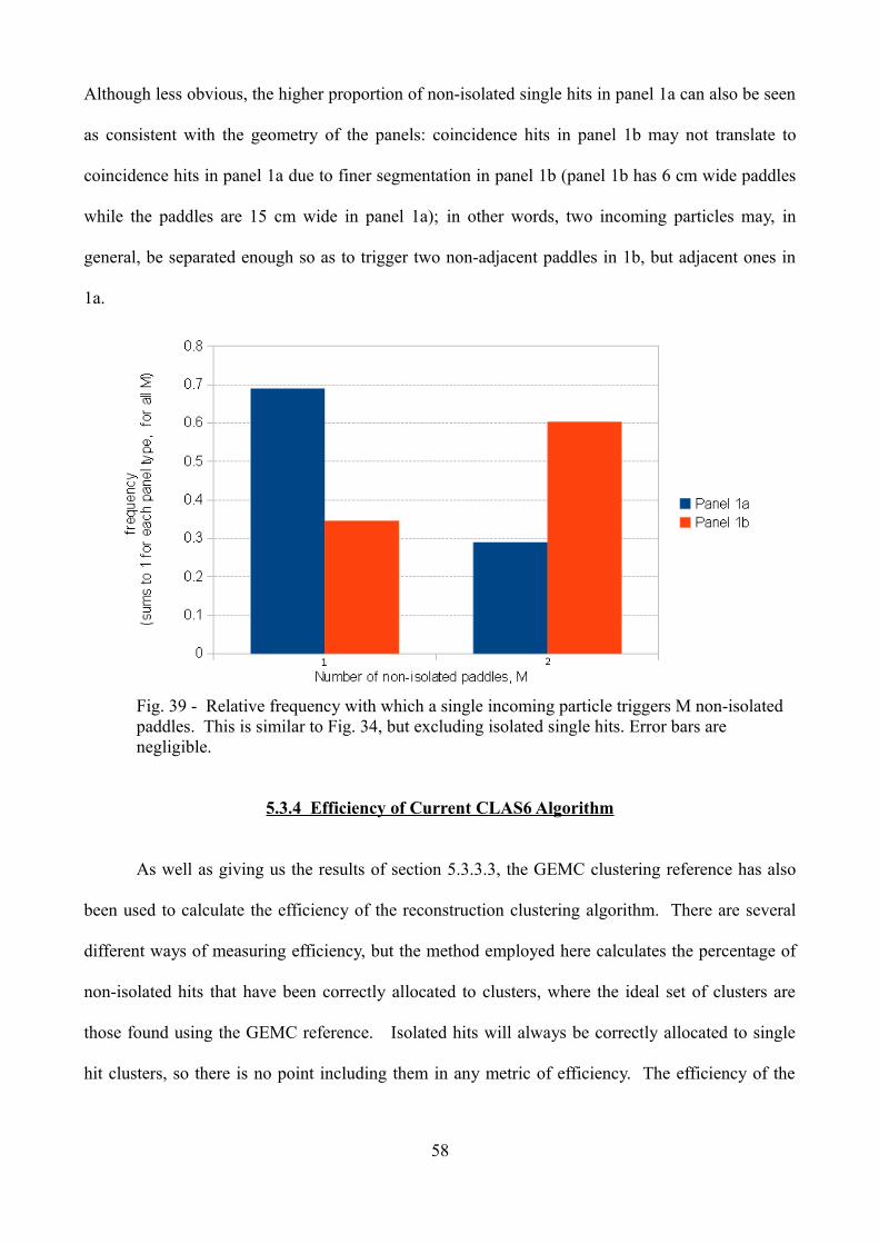
Although less obvious, the higher proportion of non-isolated single hits in panel 1a can also be seen

as consistent with the geometry of the panels: coincidence hits in panel 1b may not translate to

coincidence hits in panel 1a due to finer segmentation in panel 1b (panel 1b has 6 cm wide paddles

while the paddles are 15 cm wide in panel 1a); in other words, two incoming particles may, in

general, be separated enough so as to trigger two non-adjacent paddles in 1b, but adjacent ones in

1a.

Fig. 39 - Relative frequency with which a single incoming particle triggers M non-isolated paddles. This is similar to Fig. 34, but excluding isolated single hits. Error bars are negligible.

5.3.4 Efficiency of Current CLAS6 Algorithm

As well as giving us the results of section 5.3.3.3, the GEMC clustering reference has also

been used to calculate the efficiency of the reconstruction clustering algorithm. There are several

different ways of measuring efficiency, but the method employed here calculates the percentage of

non-isolated hits that have been correctly allocated to clusters, where the ideal set of clusters are

those found using the GEMC reference. Isolated hits will always be correctly allocated to single

hit clusters, so there is no point including them in any metric of efficiency. The efficiency of the

58

CLAS6 clustering algorithm establishes a baseline against which any alterations can be compared.

Unfortunately, it is not a very well defined baseline. As described in section 5.3.2, the decision

whether to cluster relies on uncertainties in time and y position, and these uncertainties in turn rely

on the set of calibration parameters given in section 3.2. The values of these calibration parameters

vary per paddle and per data run. There is no guarantee that the same values, or even the same

parameters, will be used in CLAS12. Nevertheless, it is still useful to pick a, hopefully

representative, set of calibration variables and use these to define our baseline. See App. N for

values of the calibration variables used, the same set for all paddles. The values used are the

median values of one particular set of calibration parameters used in CLAS6. The inherently

changeable nature of calibration variables suggests that it may be sensible to remove them from the

clustering algorithm altogether by using absolute differences in time and y position rather than

uncertainty multiples, see section 5.3.6.2. With the caveats stipulated above, the efficiency of the

CLAS 6 clustering algorithm is shown is Table 4. Attempts to improve these efficiencies are

considered in the following section.

Percentage of correctly allocated non-isolated hits versus GEMC reference

Panel 1a Panel 1b Panel 2

53.0% 73.8% 78.9% +- 0.2% +- 0.1% +- 0.1%

Table 4 – Efficiency of CLAS 6 algorithm per panel type

59

5.3.5 Potential Alterations to the CLAS6 Algorithm

5.3.5.1 Optimal Uncertainty Multiples per Panel

From Figs 38 and 39, it seems likely that the different panel types should not be using the

same set of uncertainty multiples when deciding if two adjacent paddle hits are related and hence

worthy of clustering (see section 5.3.2, question 1). To investigate this, code was written to find the

optimal uncertainty multiples for each panel type. For a range of time uncertainty multiples and y

uncertainty multiples, the number of correct 'hits are related' decisions versus the GEMC reference

were counted, and the peak values identified. As a reminder, hits are considered related if the

breach condition of section 5.3.3.2 occurs. Results are shown pictorially in Figs 40-42. These

graphs show, for a given y and time multiple, the ratio of correct clustering decisions made with

these multiples over the number of correct decisions made with the CLAS6 multiples. Values on

the vertical axis greater than 1 correspond to improvement versus CLAS6, those below, a

deterioration. The peak values are tabulated separately in Table 5.

Fig 40 – Panel 1a variation in number of correct clustering decisions versus CLAS 6 with y and time uncertainty multiples.

60

Fig 41 – Panel 1b variation in number of correct clustering decisions versus CLAS 6 with y and time uncertainty multiples.

Fig 42 – Panel 2 variation in number of correct clustering decisions versus CLAS 6 with y and time uncertainty multiples.

61

Panel 1a Panel 1b Panel 2

time uncertainty multiple 2.0 4.5 1.9+-0.1 +-0.3 +-0.1

y uncertainty multiple 0.13 0.79 0.35+-0.01 +-0.03 +-0.03

Table 5 – Optimal uncertainty multiples leading to the greatest number of correct clustering decisions versus GEMC reference.

When using these optimal uncertainty multiples in the reconstruction algorithm, the

clustering efficiency improves on all panels, but most significantly for Panel 1a, see Table 6.

Panel 1a Panel 1b Panel 2

Clustering efficiency (%) 69.1 74.8 86.4+-0.1 +-0.1 +-0.4

Change in efficiency +30.4 +1.3 +9.5versus CLAS 6 (%) +-0.6 +-0.1 +-0.6

Table 6 – Absolute and relative clustering efficiency improvements when using optimal uncertainty multiples rather than CLAS 6 multiples.

5.3.5.2 Variable Cluster Size

Fig 38 shows that a small proportion of the time a single incoming particles triggers more

than 2 paddles, therefore it seems possible that increasing the cluster size could increase clustering

efficiency. To investigate this, the existing CLAS 6 algorithm was altered so that the cluster length

could vary such that all the hits in a chain of adjacent related paddle hits are made into a cluster.

Results are shown in Table 7. Panel 1b improves, the other panels get worse. This worsening in

efficiency can be explained by the fact that we are not using the optimal uncertainty multiples of

section 5.3.5.1, hence the result of increasing the cluster size is to incorrectly allocate more hits to

larger clusters.

62

Panel 1a Panel 1b Panel 2

Clustering efficiency (%) 48.9 78.6 78.1+-0.2 +-0.1 +-0.5

Change in efficiency -7.7 +6.3 -1.0versus CLAS 6 (%) +-0.1 +-0.1 +-0.6

Table 7 - Absolute and relative clustering efficiency improvements when using variable cluster sizes rather than clusters of size 2.

5.3.5.3 Optimal Uncertainty Multiples and Variable Cluster Size

By combining optimal uncertainty multiples and variable cluster size, results are improved over

using either one alone, as shown in Table 8. Fig. 43 compares all the results given in section 5.3.5

Note that even with these optimizations, the CLAS12 clustering algorithm is, at worst, only about

69% efficient, but is still significantly improved over CLAS6.

Panel 1a Panel 1b Panel 2

Clustering efficiency (%) 69.1 79.6 86.8+-0.2 +-0.1 +-0.6

Change in efficiency +30.4 +7.8 +10.0versus CLAS 6 (%) +-0.6 +-0.2 +-0.5

Table 8 – Absolute and relative clustering efficiency improvements when using both variable cluster sizes and optimal uncertainty multiples.

63

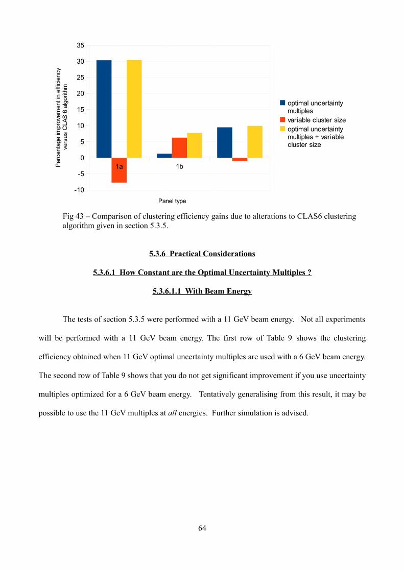
Fig 43 – Comparison of clustering efficiency gains due to alterations to CLAS6 clustering algorithm given in section 5.3.5.

5.3.6 Practical Considerations

5.3.6.1 How Constant are the Optimal Uncertainty Multiples ?

5.3.6.1.1 With Beam Energy

The tests of section 5.3.5 were performed with a 11 GeV beam energy. Not all experiments

will be performed with a 11 GeV beam energy. The first row of Table 9 shows the clustering

efficiency obtained when 11 GeV optimal uncertainty multiples are used with a 6 GeV beam energy.

The second row of Table 9 shows that you do not get significant improvement if you use uncertainty

multiples optimized for a 6 GeV beam energy. Tentatively generalising from this result, it may be

possible to use the 11 GeV multiples at all energies. Further simulation is advised.

64

1a 1b

-10

-5

0

5

10

15

20

25

30

35

optimal uncertainty multiplesvariable cluster sizeoptimal uncertainty multiples + variable cluster size

Panel type

Per

cent

age

impr

ovem

ent i

n ef

ficie

ncy

ver

sus

CLA

S 6

alg

orith

m

Panel 1a Panel 1b Panel 2

Clustering efficiency when using 71.2 85.6 82.911 GeV optimal uncertainties (%) +-1.0 +-1.0 +-3.6

Clustering efficiency when using 71.2 85.7 82.96 GeV optimal uncertainties (%) +-1.0 +-1.0 +-4.0

Table 9 – Clustering efficiency when using optimal 11 GeV and 6 GeV uncertainty multiples when the beam energy is 6 GeV.

5.3.6.1.2 With ADC discriminator threshold

The optimal uncertainty multiples vary marginally with ADC discriminator threshold. Once

the discriminator threshold is known for CLAS12, the optimal uncertainty multiples can be

recalculated, if necessary.

5.3.6.2 Uncertainty Multiples or Absolute Differences ?

As shown in section 5.3.5.1, the use of optimal uncertainty multiples could be used to

improve clustering efficiency. However, for practical reasons, it may be preferable not to use

uncertainty multiples, optimized or not. The tests of section 5.3.5.1 were somewhat artificial. If

the paddles were to have a widely varying set of calibration parameters, leading to an equally

widely varying set of uncertainties, the clustering efficiency may be significantly lowered (one

specific uncertainty multiple is unlikely to suit all uncertainties). To maintain peak efficiency, you

would have to recalculate the optimum uncertainty values whenever the calibration variables

changed. In any case, the efficiency is likely to vary, even if optimized. To avoid all these

potential issues, instead of using uncertainty multiples, it would be possible to use absolute

differences. The use of absolute differences is explained below, by re-answering some of the

questions from section 5.3.2.

(2) How are two adjacent paddle hits considered related and hence worthy of clustering?

Two adjacent paddle hits are considered related if the absolute difference in sector y

65

positions is less than a pre-determined value AND the absolute difference in time is less than

another pre-determined value. These pre-determined absolute differences are specific to a panel

type and are found using an equivalent method to that described at the start of section 5.3.5.1 – by

maximizing the number of 'hits are related' decisions versus the GEMC reference over a range of

absolute differences in y and time. See Figs 44-46 (equivalent to Figs 40-42), for graphs of

variation in number of 'hits are related' decisions versus CLAS 6, and Table 10 (equivalent to Table

5), for the optimal absolute differences that emerge from these graphs.

Fig. 44 - Panel 1a variation in number of correct clustering decisions versus CLAS 6 with y and time absolute differences.

66

Fig. 45 - Panel 1b variation in number of correct clustering decisions versus CLAS 6 with y and time absolute differences.

Fig. 46 - Panel 2 variation in number of correct clustering decisions versus CLAS 6 with y and time absolute differences.

67

Panel 1a Panel 1b Panel 2

time difference (ns) 3.4 5.2 3.3+-0.2 +-0.3 +-0.1

y difference (cm) 3.7 20.3 9.4+-0.2 +-1.1 +-0.7

Table 10 – Optimal absolute differences leading to the greatest number of correct clustering decisions versus GEMC reference.

(3) If there are more adjacent paddle hits than the maximum cluster size, which of the hits are

combined?

In answering this question, the cluster size is assumed to be variable up to a maximum

cluster size, as this was shown to be beneficial in section 5.3.5.2. If there are more hits than the

maximum cluster size, the algorithm will only combine the maximum cluster size number of hits.

In deciding which hit to drop from the cluster, the end pairs are compared. The first pair (with the

lowest paddle IDs) will be included in the cluster if (1) the absolute time difference for the second

pair is greater than the absolute time difference for the first pair, OR (2) the absolute y difference for

the second pair is greater than the absolute y difference for the first pair.

This alternative method, based on absolute differences rather than uncertainty multiples was

implemented in code. The clustering efficiency obtained when using these absolute differences

plus variable cluster size is shown in Table 11. Taking into account the uncertainties, the

improvements shown in Table 11 are the same as those shown in Table 8 when using uncertainty

multiples plus variable cluster size. However, these efficiency numbers are independent of the

values of the calibration variables.

Panel 1a Panel 1b Panel 2

Clustering efficiency (%) 68.9 80.0 87.4+-0.2 +-0.2 +-0.2

Change in efficiency +30.0 +8.4 +10.8versus CLAS 6 (%) +-0.5 +-0.2 +-0.7

Table 11 – Absolute and relative clustering efficiency when using optimal absolute differences and variable cluster size. Compare with table 8.

68

5.3.6.3 Calculating Cluster Parameters from the Constituent Hits

If using clusters of size 2 or more, it is necessary to adapt the method by which the

individual parameters of the hits – time, energy and position - are combined when creating a

cluster. It is possible to do this in a number of different ways. The most obvious approach is to use

an extended version of the method using in CLAS6, described in section 5.3.2, question 4. Thus,

the averages, energy-weighted or regular, are taken across all N hits rather than 2 hits. However, it

may be preferable to use the time and position from the earliest hit in the cluster, with energy

remaining a simple sum. The distribution of differences between the earliest time in a cluster and

the energy-weighted time is shown in Fig. 47. Given that the time resolution of FTOF paddles is

between 60ps and 150ps [2], and taking the worst of these paddle time resolutions to be

approximately equal to the resolution of the time difference, this means that in at least 30% of cases

the time difference is greater than the resolution and can therefore be distinguished. Using the

earliest hit values would probably provide a closer tie up between the cluster time and position, and

the time and position calculated from an extrapolated track from the drift chamber that will be used

when matching data between tracking and the TOF. This can be tested when a tracking input

becomes available.

Fig 47 – Illustration of significant differences between the earliest hit time in a cluster (of size 2 hits or more) and the energy-weighted average time.

69

5.3.6.4 Limit on Cluster Size

For maximum efficiency, it would be ideal to allow a variable length cluster to be arbitrarily

long. In practice, it might be beneficial to put a limit on it. For example, if you want the cluster

output to contain the statuses of all the composing hits - as CLAS6 does - and you happen to have 6

or more hits in the cluster, then the output would not fit in a single Java integer. Fig 48 shows the

efficiency implications on panel 1b of using a reduced cluster size versus using one of size 17 hits,

which is the maximum cluster size found in this sample. A cluster of size of 5 retains 82% of the

efficiency benefit of one of size 17, plus you would still be capturing the majority of energy in the

cases that a single particle triggers 6 or more paddles, which are very rare events in any case, see

Fig. 38.

Fig. 48 – Efficiency implications on panel 1b of using a limited maximum cluster size. The CLAS 6 clustering algorithm, which uses a maximum cluster size of 2 hits, is taken as the baseline i.e. 0% efficiency improvement. The optimal improvement in efficiency happens with a maximum cluster size of 17 hits; this is defined as 100% efficiency improvement.

70

2 4 6 8 10 12 14 16 180

102030405060708090

100

Max cluster size (hits)

Per

cent

age

effic

ienc

y im

prov

emen

t ver

sus

CLA

S 6

alg

orith

m(w

ith N

=17

set t

o 10

0%)

5.3.6.5 – Verification with Production Data

Given that the results here are based on simulations, assumptions and approximations, it will

obviously be necessary to verify them with production data, in as much is possible, before

committing to any changes on a permanent basis. A point not mentioned so far is that GEMC

outputs total flight time, not the smaller proportion of this that would be output by the real CLAS12

detector. The uncertainties in time depend, to some extent, on the value of the time, hence the

optimal time uncertainty multiple may have different values for the real detector. Another issue is

that GEMC can output multiple hits on the same paddle in a single event, something that the real

detector is unable to do and something that may have a small effect on the results. Finally, the

version of GEMC used did not contain the final FTOF geometry. At some point all these issues will

be resolved in GEMC; the clustering parameters should then be re-calculated. Instructions on how

to do this can be found in [16].

5.3.7 Proposed Defaults for the CLAS12 Algorithm

Given the evidence presented in sections 5.3.1 - 5.3.6, the proposed defaults for the CLAS12

clustering algorithm are as follows:

• The decision as to whether two hits are related and hence worthy of clustering should be

based on absolute differences, not uncertainty multiples (section 5.3.6.2).

• In either case, the absolute differences, or uncertainty multiples, should be unique to the

panel type (sections 5.3.5.1 and 5.3.6.2).

• The maximum cluster length should be increased to 5 hits (sections 5.3.5.2 and 5.3.6.4).

• If further study shows it beneficial, then cluster position and time should come from the

earliest hit in a cluster (section 5.3.6.3).

71

5.3.8 Implementation of Configurable CLAS12 Algorithm

The class PanelReconstructionCLAS12 implements the CLAS12 clustering algorithm in a

flexible way, such that the exact behaviour is determined by a set of calibration parameters that are

specified in the calibration service xml, see App. D for the proposed calibration service XML. This

mechanism allows for the use of the proposed defaults of section 5.3.7, or the existing CLAS6

algorithm, described in section 5.3.2, or some other hybrid, without changing the code.

PanelReconstructionCLAS12 works by first finding chains of related adjacent paddle hits,

then combining those into one or more clusters. When determining if two adjacent paddle hits are

related, this can be done using two methods. If RELATED_METHOD equals “uncertainty”, then

two hits are considered related using uncertainty multiples, as described in section 5.3.2, question 1.

The uncertainty multiples to be used are defined per panel in

PANEL_XX_UNCERTAINTY_MULTIPLE_TIME and

PANEL_XX_UNCERTAINTY_MULTIPLE_YPOSITION, where XX is replaced by 1A,1B or 2. If

RELATED_METHOD equals “absolute”, two hits are considered related using absolute differences,

as described in section 5.3.6.2, question 2. The absolute differences to be used are defined per

panel in PANEL_XX_DIFFERENCE_TIME and PANEL_XX_DIFFERENCE_YPOSITION,

where XX is replaced by 1A,1B or 2. If COMBINE_ALL_HITS is equal to “true”, then all the hits

in the chain of related adjacent paddle hits are combined into a cluster, however many hits there are.

If COMBINE_ALL_HITS is equal to “false”, then the chain of related adjacent paddle hits are

combined into clusters of maximum length MAX_CLUSTER_LENGTH, where

MAX_CLUSTER_LENGTH is five or less. If there are less than or equal to

MAX_CLUSTER_LENGTH hits in the chain of related adjacent paddle hits, then all the hits in the

chain are made into a cluster. If there are more than MAX_CLUSTER_LENGTH hits in the chain

of related adjacent paddle hits then if the first set of MAX_CLUSTER_LEGNTH hits is better

matched than the second overlapping set, the first set is made into a cluster. There are two methods

72

to decide which set is better matched. If RELATED_METHOD equals “uncertainty”, the CLAS6

method is used (see section 5.3.2, question 3), such that the first set (closest to beam line) is made

into a cluster if the final pair of hits (furthest from beam line) has greater combined time

uncertainty, or greater combined sector y position uncertainty, than the first pair. If

RELATED_METHOD equals “absolute”, then the first set is made into a cluster if the final pair of

hits has greater absolute difference in sector y positions, or greater absolute time difference in

times, than the first pair. When combining hits into a cluster, if COMBINATION_METHOD

equals “average”, then hit positions and times are combined into a cluster position and time using

averages, as in CLAS6, see section 5.3.2, question 4. If COMBINATION_METHOD equals

“earliest”, then the cluster position and time comes from the earliest hit in the cluster. In either

case, cluster energy is the sum of the hit energies, the cluster paddle ID is the cluster of the first hit

in the cluster, and the cluster status is calculated from the addition of terms of the form 100(index of hit)

* (status of hit), where the addition is performed over all hit indices, where the hit index ranges

from zero to the number of hits in a cluster minus one, with the hit closest to the beam line having

index zero.

Table 12 shows how to configure the CLAS12 clustering algorithm to work like CLAS6 did.

Variable Name Value

PANEL_XX_UNCERTAINTY_MULTIPLE_TIME 3

PANEL_XX_UNCERTAINTY_YPOSITION 3

MAX_CLUSTER_LENGTH 2

RELATED_METHOD “uncertainty”

COMBINATION_METHOD “average”

Table 12 - Values of the clustering variables that make the CLAS12 clustering algorithm work like the CLAS6 clustering algorithm.

73

5.4 Additional Prototyping

As particles mostly trigger paddles in both panels 1a and 1b, an attempt was made to tie up

clusters in panel-1a with clusters in panel-1b with a view to combining their parameters into a

'supercluster'. This was done by projecting the panel-1b hit point in a straight line onto panel-1a,

and then looking for the panel-1a hit closest to this projected hit point. This idea was subsequently

abandoned as the number of clusters in panel-1a and 1b only matched 30% of the time, and to

match accurately, it needed a tracking input so that the projection could be done in the direction of a

particle's travel. In any case, the Event Builder service will tie hits to tracks for all detector

subsystems, so this functionality does not need to be performed within the FTOF service.

5.5 Testing

Testing of the FTOF reconstruction service has taken a number of forms, listed below. Any

areas not specifically addressed by the methods given have been tested using adhoc manual testing.

• Many of the equations outlined in section 3.2 (and the uncertainty equations that go along

with them) were cut and paste directly from the CLAS6 software, with no, or only minor,

changes to convert from C to Java. These equations are essentially pre-tested, having been

in use for many years. In any case, the validity of the existing code was rechecked.

• The generation and verification of the simulation results of section 4 provided a basic check

that GEMC data was being read in, stored and output correctly.

• The exact GEMC values for hit time, energy and position were compared with the

reconstruction output for 20000 simulated events, created using the process outlined in

section 3.3 with the beam energy set to 11 GeV. This tested that the reverse and forward

reconstruction algorithms were doing the same thing. Results are given in Figs 49-53. Note

that the reconstruction values are expected to be different from the GEMC values for two

74

reasons. Firstly, the GEMC energy and time are exact, whilst the reconstruction uses

digitized energy and time. Secondly, as stated in section 3.2, the reconstruction has to

assume that hits are located on the centre line of the paddle. The wider shapes of graphs 51

and 53 are determined by this centre line assumption (and to a much lesser extent,

digitization), the narrower, more regular shapes of the other graphs by digitization alone.

• The FTOF service has been successfully deployed as part of a reconstruction chain similar

to, but simpler than, that shown in Fig. 12 in section 3.1. The chain ran successfully on fifty

computing nodes.

Fig. 49– difference in reconstruction and GEMC hit times.

Fig. 50 – difference in reconstruction and GEMC hit energy deposited.

75

Fig. 51 – difference in reconstruction and GEMC x hit position (sector coordinates)

Fig. 52 – difference in reconstruction and GEMC y hit position (sector coordinates)

Fig. 53 – difference in reconstruction and GEMC z hit position (sector coordinates)

76

5.6 Future Work

The FTOF reconstruction service is work in progress. Future work on the service can be

divided into compulsory tasks, and tasks that may arise if certain assumptions turn out to be invalid.

The main compulsory tasks include:

• All calibration equations and variables, as defined in section 3.2, and implemented in

PaddleReader and PaddleReconstruction, must be checked and if necessary updated for

CLAS12. This should be done by a calibration expert. This may have knock on implications

for the format of the calibration xml, the proposed format of which is given in App. D, and

the Calibration package classes.

• The service must be switched over to using the Calibration service. Code exists to do this,

but is currently bypassed.

• Reading in and processing of the tracking input from the Event Builder service (see section

3.1) must be implemented, for use in case of missing or invalid TDC data, as outlined in

section 3.2, step 3. It is known that the Event Builder service will provide information on

the location and direction of tracks at the face of the FTOF panels, but not the exact input

format. Code exists in CLAS6 to match an input track to a paddle, if this is not done by the

Event Builder service.

• As stated in section 5.3.6.3, the validity of taking cluster parameters from the earliest hit of a

cluster must be validated.

• As stated in section 5.3.6.5, the clustering parameters used in the PanelReconstruction must

be recalculated when GEMC is as lifelike as it is going to get.

• As stated in section 5.3.6.5, the clustering algorithm must be verified with production data.

The assumptions that must be checked include:

• The input EVIO will be formatted as per App. B, in particular for a single event, the input

evio will only contain one set of ADC/TDC left/right values for a given paddle per event.

77

GEMC can output multiple hits on a single paddle in a single event. The reconstruction

actively ignores all but the first set of readings it processes on a given paddle.

• The calibration service will adjust the calibration parameter T0 (used in eqn. 2, section 3.2)

with (1) panel to panel, (2) paddle to paddle and (3) left / right adjustments as per CLAS6.

A more detailed list of compulsory tasks and assumptions is available at [15].

78

6. CLAS12 CTOF Reconstruction Service

6.1 Overview

Barring differences due to the geometry of their respective hardware (see section 2.1), the

CTOF reconstruction service is identical to the FTOF reconstruction service. This section will only

highlight differences between the two services; where something is identical to FTOF, it will be

ignored.

As shown in Fig. 54, the data flowing in and out of the CTOF service is similar to that

shown in Fig. 25 for FTOF. The main difference is that there is only one set of input banks, defined

in App. G. The output banks are identical, except for the fact that CTOF does not have panels or

sectors, hence does not output a panel ID or a sector ID, see App. J. The format of the proposed

CTOF calibration and geometry service XMLs are given in appendices H and I, respectively.

Currently, neither the calibration nor geometry service exists for CTOF, so all values are hard-

coded.

Fig. 54 – CTOF reconstruction service input and output

79

6.2 Code differences versus FTOF

This section outlines the coding differences between FTOF and CTOF. There is a more

detailed list of the code dependencies and equivalencies between FTOF and CTOF in App. O.

• The most obvious difference is that CTOF does not have sectors, hence the

SectorReconstruction class does not exist and sector coordinates are not used, CLAS

coordinates are. The sector and CLAS coordinate systems were defined in Fig. 7 in section

2.1.2. CTOF paddles are arranged with their length along a different axis to FTOF, hence

sector y in FTOF becomes CLAS z in CTOF, CLAS z being along the beam. Consequently,

the CLAS x and y coordinates of a hit are determined by the position of the centre of the

paddle. In the FTOF service, the sector x and z coordinates of a hit are determined by the

centre of the paddle.

• CTOF does not have panels either, though the cylindrical arrangement of paddles in CTOF

can be seen as a single panel that curves rounds to meet itself. Hence, the

PanelReconstructionCLAS12 class becomes the CylinderReconstruction class, which is

configurable in a similar manner to that given in section 5.3.8. In a cylinder, clustering is

allowed between the two edges of the panel, so new code has been written that does this.

• As the calibration and geometry xmls are in a different format from FTOF, the code to read

them is different, as are the classes to store them in. Likewise with code to input and output

to EVIO, the banks having slightly different definitions.

6.3 Testing

The CTOF reconstruction service has been tested in an identical manner to the FTOF

service, therefore the comments given in section 5.4 apply here. Graphs equivalent to Figs 49-53,

which show the distributions in the differences between reconstruction and GEMC values in time,

energy and position are given in Figs 55-59. They show that the reverse and forward reconstruction

80

algorithms do the same thing within reasonable limits. Graphs 57 and 58 have shapes due to the

centre line assumption, the other graphs have narrower, more regular shapes due to digitization

alone.

Fig. 55 – difference in reconstruction and GEMC hit time

Fig. 56 – difference in reconstruction and GEMC hit energy

81

Fig. 57 – difference in reconstruction and GEMC hit x position (CLAS coordinates)

Fig. 58 – difference in reconstruction and GEMC hit y position (CLAS coordinates)

Fig. 59 – difference in reconstruction and GEMC hit z position (CLAS coordinates)

82

6.4 Future Work

The CTOF reconstruction service is work in progress. Future work on the service is

essentially the same as for FTOF specified in section 5.5. In addition, CTOF must be switched over

to using the CTOF geometry service. Code exists to do this, but is currently bypassed because the

CTOF geometry service is not yet available. Also, when it becomes possible (when the GEMC

output contains momentum at the CTOF paddles), the ConfigCylinderReconstruction class must be

used to find the optimal CTOF clustering parameters, in a similar way to how

ConfigPanelReconstructionCLAS12 was used to find optimal FTOF clustering parameters. A

more detailed list of CTOF specific compulsory tasks and assumptions is available at [15].

83

7. Summary

Jefferson Laboratory is currently increasing the beam energy of CEBAF from 5.7 to 11 GeV.

As part of this upgrade, the detector in experimental Hall B, CLAS12, is being upgraded. CLAS12

has two subsystems - CTOF and FTOF - which measure the flight time of particles in the central

and forward detectors, respectively. Simulation of these detectors has yielded some insights into

how they will behave when the CLAS12 detector is switched on in 2016, including distributions in

hit position, time, and energy deposited. Simulation has also been used to shape the development of

new CLARA services that reconstruct the raw data from the TOF detectors. The operation and

organisation of these services has been described in detail, highlighting how they compare to each

other and to the existing CLAS6 FTOF reconstruction software on which they are based. The

CTOF and FTOF services are very similar to each other, with only minor differences due to their

respective geometries. In terms of behaviour, the main difference CLAS6 versus CLAS12 is the

clustering algorithm that has been redesigned. Simulation showed that clustering is more efficient

if each FTOF panel is treated separately and if clusters are created from more than two hits. These

features have been introduced in a configurable clustering algorithm. On the technical side, the

programming language has been switched from C to Java, and the software now runs in the CLARA

platform. Although good progress has been made on the TOF services, work still remains to be

done. All calibration variables and equations must be updated for CLAS12. Both services must be

switched to using the Calibration service and CTOF must be switched to use the Geometry service

as well. In addition, both services must implement the use of a tracking input which will at some

point be provided by the Event Builder service.

84

8. References

[1] The US Nuclear Science Advisory Committee, 'The Frontiers of Nuclear Science: A Long Range Plan' (2007)

[2] B. Mecking, et al., (The CLAS Collaboration), ‘The CEBAF Large Acceptance Spectrometer’,Nucl. Instr. and Meth., 503/3, 513 (2003).

[3] C.W. Leemann, W. Christoph, D. R. Douglas, and G. A. Krafft, "The Continuous Electron Beam Accelerator Facility: CEBAF at the Jefferson Laboratory.", Annual Review of Nuclear and Particle Science, 51.1, 413 (2001)

[4] www.jlab.org/12-gev-upgrade , accessed on 01/06/2013

[5] 'CLAS12 Technical Design Report', version 5.1, www.jlab.org/Hall-B/ clas12 _tdr.pdf , accessed on 01/06/2013

[6] E.S. Smith, et al, 'The time-of-flight system for CLAS', Nucl. Instr. and Meth., A432, 265 (1999)

[7] S.J. Taylor, 'Radiative Decays of Low-Lying Excited-State Hyperons', Ph.D. Thesis, Rice University, USA (2000), available at https://clasweb.jlab.org/wiki/index.php/CLAS12_Time-of-Flight_Software

[8] K. Loukachine, 'Electroproduction of the φ(1020) Vector Meson at 4GeV', Ph.D. Thesis, Virginia Polytechnic Institute and State University, USA (2000), available at the same place as [7]

[9] G.F. Knoll, 'Radiation Detection and Measurement', 3rd edition, Wiley (2000)

[10] V. Gyurjyan, et al., "CLARA: A Contemporary Approach to Physics Data Processing.", Journal of Physics: Conference Series, 331/3 (2011)

[11] http://www.jlab.org/Hall-B/clas12-web/ , accessed on 01/06/2013

[12] 'CLAS12 software document; Hall B 12 GeV upgrade', http://www.jlab.org/Hall-B/clas12-software.pdf , accessed on 01/06/2013

[13] https://gemc.jlab.org/gemc/Documentation/Entries/2011/3/18_The_LUND_Format.html , accessed on 01/06/2013

[14] https://userweb.jlab.org/~carman/ftof/notes/ftof_geom.pdf , accessed on 02/11/2013

[15] https://clasweb.jlab.org/wiki/index.php/CLAS12_Time-of-Flight_Software , file FTOFCTOFstilltodo.doc , edited on 15/12/2013

[16] https://clasweb.jlab.org/wiki/index.php/CLAS12_Time-of-Flight_Software , fileFTOFREADME.doc , edited on 15/12/2013

[17] http://www.crystals.saint-gobain.com/uploadedFiles/SG-Crystals/Documents/SGC%20BC400-404-408-412-416%20Data%20Sheet.pdf , accessed on 20/01/2014

[18] J. Walker et al, 'Fundamentals of Physics', 8th edition, Wiley, 2008

[19] C. Quigg, "Elementary Particle Physics: Discoveries, Insights, and Tools", in Quarks, Quasars and Quandries, Ed. G. Aubrecht, American Association of Physics Teachers (1987)

85

9. Appendices

Appendix A – Definition of CLAS6 Status Integer ( also used in CLAS12 )

Value: Mneumonic: Meaning:

1 TDCL_GOOD Only tdcl 2 ADCL_GOOD Only adcl. Discarded. 3 LEFT_OK tdcl,adcl 4 TDCR_GOOD Only tdcr 5 TDCS_ONLY tdcl,tdcr 6 ADCL_TDCR Self-evident! 7 LEFT_OK_NO_ADCR tdcl,adcl,tdcr 8 ADCR_GOOD Only adcr. Discarded.

9 TDCL_ADCR Self-evident! 10 ADCS_ONLY adcl,adcr. Discarded. 11 LEFT_OK_NO_TDCR tdcl,adcl,adcr 12 RIGHT_OK tdcr,adcr 13 RIGHT_OK_NO_ADCL tdcl,tdcr,adcr 14 RIGHT_OK_NO_TDCL adcl,tdcr,adcr 15 BOTH_OK tdcl,adcl,tdcr,adcr.

Appendix B – Format of Input EVIO Banks for the FTOF Service

There are three sets of input EVIO banks, one set for each of the panel types – 1a, 1b, and 2.

Bank set Tag

Panel-1a 60Panel-1b 70Panel-2 80

Banks found in the GEMC output and assumed to be present in the real detector output:

Name Num Format Description

Sector ID 21 Integer Sector ID (1-6), as defined in Fig. 7Paddle ID 22 Integer Paddle IDADCL 23 Integer Left ADC value (channels)ADCR 24 Integer Right ADC value (channels)TDCL 25 Integer Left TDC value (channels)TDCR 26 Integer Right TDC value (channels)

Additional banks found in GEMC output only:

Name Num Format Description

Energy deposited 1 Double Energy deposited (MeV)X position 2 Double X position, CLAS coords (mm)

86

Y position 3 Double Y position, CLAS coords (mm)Z position 4 Double Z position, CLAS coords (mm)Time 8 Double Time (ns)Local X position 5 Double X position, local coords (mm)Local Y position 6 Double Y position, local coords (mm)Local Z position 7 Double Z position, local coords (mm)Entrance energy 13 Double Entrance energy (MeV)Particle ID 9 Double Lund particle ID [13]X momentum 18 Double X momentum, CLAS coords (mm)Y momentum 19 Double Y momentum, CLAS coords (mm)Z momentum 20 Double Z momentum, CLAS coords (mm)

Appendix C – Geometry XML for the FTOF Service

Example XML (including data from one panel only)

<geometry><forward_tof>

<panels_parms length_units="cm" coordinate_system="sector"><panel sector="0" panel="1a" npaddles="23" dist2tgt="684.81" norm_phi="0"

norm_theta="0.436332" paddle_phi="1.5708" paddle_theta="1.5708" paddle_width="15" paddle_thickness="5" paddle_extent_x="15.7077" paddle_extent_z="10.8708">

<paddle_centers><x>62.1588 75.8993 89.6398 103.38 117.121 130.861 144.602

158.343 172.083 185.824 199.564 213.305 227.045 240.786 254.526 268.267 282.007 295.748 309.488 323.229 336.969 350.71 364.45</x>

<y>0 0 0 0 0 0 0 0 0 0 0 0 0 0 0 0 0 0 0 0 0 0 0</y><z>726.619 720.212 713.805 707.397 700.99 694.583 688.175

681.768 675.361 668.953 662.546 656.139 649.732 643.324 636.917 630.51 624.102 617.695 611.288 604.88 598.473 592.066 585.658</z>

</paddle_centers><paddle_lengths>32.28 48.13 63.98 79.83 95.68 106.576 122.43 138.284

154.138 169.992 185.846 201.7 217.554 233.408 249.262 265.116 280.97 296.824 312.678 328.532 344.386 360.24 376.094</paddle_lengths>

</panel>OTHER PANELS GO HERE

</panels_parms></forward_tof>

<geometry>

Definition of parameters

sector sector this panel belongs to minus one (0-5)panel panel type (1a,1b,2)npaddles number of paddles in paneldist2tgt length of a line perpendicular to the panel, starting half way through the

thickness of the panel and ending at the CLAS origin (0,0,0)norm_phi phi angle of vector normal to panel, pointing away from targetnorm_theta theta angle of vector normal to panel, pointing away from targetpaddle_phi phi angle of vector pointing along length of paddle, left to right, or in sector

1 from negative to positive ypaddle_phi theta angle of vector pointing along length of paddle, left to right, or in sector

1 from negative to positive ypaddle_width width of paddle (width of face oriented towards target, same for all paddles in

panel)paddle_thickness thickness of paddle (i.e. depth of material away from target)paddle_extent_x extent of paddle projected along x axis

87

paddle_extent_z extent of paddle projected along z axispaddle_centre, x/y/z volume centre of paddlepaddle_length length of paddle (in sector 1 this is extent of paddle in y, paddles get longer

with increasing x)

Appendix D – Proposed Calibration XML for the FTOF Service

Note that the proposed format here is based on CLAS6 calibration variables and may have to change when the CLAS12 variables are decided upon.

Example xml (including data for one panel only and not showing values per paddle)

<calibration><forward_tof>

<detector ref_adc="600" pulser="1" tdc_max="8192" adc_max="8192" dedx_nmip="1.998" disc_thresh="35" adc_jitter="1" tdc_jitter="1" related_method="absolute" combine_all_hits="false" max_cluster_length="5" combination_method="earliest" panel1a_diff_time = "3.4" panel1a_diff_y="0.6" panel1b_diff_time="5.2" panel1b_diff_y="20.3" panel2_diff_time="3.3" panel2_diff_y="9.4" />

<panel sector="0" panel="1a" npaddles="23"><atten>

<left></left><right></right>

</atten><atten_u>

<left></left><right></right>

</atten_u><nmip_adc>

<left></left><right></right>

</nmip_adc><nmip_adc_u>

<left></left><right></right>

</nmip_adc_u><ped>

<left></left><right></right>

</ped><ped_u>

<left></left><right></right>

</ped_u><status>

<left></left><right></right>

</status><swap_tdc>

<left></left><right></right>

</swap_tdc><swap_adc>

<left></left><right></right>

</swap_adc><t0>

<left></left><right></right>

</t0><t1>

<left></left><right></right>

</t1><t2>

<left></left><right></right>

</t2><t0_u>

<left></left>

88

<right></right></t0_u><t1_u>

<left></left><right></right>

</t1_u><t2_u>

<left></left><right></right>

</t2_u><veff>

<left></left><right></right>

</veff><veff_u>

<left></left><right></right>

</veff_u><walk0>

<left></left><right></right>

</walk0><walk1>

<left></left><right></right>

</walk1><walk2>

<left></left><right></right>

</walk2><walk0_u>

<left></left><right></right>

</walk0_u><walk1_u>

<left></left><right></right>

</walk1_u><walk2_u>

<left></left><right></right>

</walk2_u><y_offset></y_offset>

</panel>OTHER PANELS GO HERE

</forward_tof></calibration>

Definition of parameters

ref_adc ADCREF in eqn. (4), section 3.2pulser PULSER in eqn. (2), section 3.2tdc_max maximum TDC value in channelsadc_max maximum ADC value in channelsdedx_nmip DEDXNMIP in eqn. (1), section 3.2disc_thresh DISCTHRESH in eqn. (3), section 3.2adc_jitter uncertainty in ADC value in channelstdc_jitter uncertainty in TDC value in channelsrelated_method RELATED_METHOD, section 5.3.8combine_all_hits COMBINE_ALL_HITS, section 5.3.8max_cluster_length MAX_CLUSTER_LENGTH, section 5.3.8combination_method COMBINATION_METHOD, section 5.3.8panel1a_diff_time PANEL_1A_DIFFERENCE_TIME, section 5.3.8panel1a_diff_y PANEL_1A_DIFFERENCE_Y, section 5.3.8panel1b_diff_time PANEL_1B_DIFFERENCE_TIME, section 5.3.8panel1b_diff_y PANEL_1B_DIFFERENCE_Y, section 5.3.8

89

panel2_diff_time PANEL_2_DIFFERENCE_TIME, section 5.3.8panel2_diff_y PANEL_2_DIFFERENCE_Y, section 5.3.8sector sector of panel minus one (0-5)panel panel type (1a, 1b, 2)npaddles number of paddles in sectoratten ATTENL , ATTENR in eqn. 7, section 3.2nmip_adc ADCNMIP in eqn. 1, section 3.2ped PEDSETAL in eqn. 1, section 3.2status paddle status (1-3) – 1, no ADC, 2, no TDC, 3 neither ADC nor TDCswap_tdc calibration index* of paddle to swap tdc values with, or its own

calibration index if no swapping necessaryswap_adc calibration index* of paddle to swap adc values with, or its own

calibration index if no swapping necessaryt0 TO in eqn. 2, section 3.2t1 T1 in eqn. 2, section 3.2t2 T2 in eqn. 2, section 3.2veff VEFFL and VEFFR in eqn. 6, section 3.2walk0 WALK0 in eqn. 6, section 3.2walk1 WALK1 in eqn. 6, section 3.2walk2 WALK2 in eqn. 6, section 3.2yOffset YOFFSET in eqn. 6, section 3.2

Anything with “_u” attached on the end is an uncertainty in the corresponding variable without a “_u” attached to it.

Not listed are the uncertainty multiple equivalents of panel1a_diff_time etc., which are written panel1a_mult_time etc. See section 5.3.8.

* The calibration index is an integer uniquely identifying a paddle. Paddles are numbered from 1 starting with paddle 1 in sector 1, panel 1a, then, after all paddles in that panel are named, moving to sector 1, panel 1b, then sector 1, panel 2, and then the same for sector 2 and so on up to sector 6 where the last paddle has an index of 540.

Appendix E – Format of Output EVIO Banks for the FTOF Service

There are three sets of output EVIO banks:

Name Tag

Converted Raw 800Hit 810Cluster 820

The Converted Raw banks are:

Name Num Format Description

Sector ID 1 Integer Sector ID (1-6), as defined in Fig. 7Panel ID 2 Integer Panel ID (1-3) – 1a, 1 – 1b, 2 – 2, 3

90

Paddle ID 3 Integer Paddle IDPaddle Status 4 Integer Paddle status (1-15), as defined in

Appendix AEnergy Left 5 Double Left PMT energy (MeV)Energy Right 6 Double Right PMT energy (MeV)Unc Energy Left 7 Double Uncertainty in Left PMT energy (MeV)Unc Energy Right 8 Double Uncertainty in Right PMT energy (MeV)Time Left 9 Double Left PMT time (ns)Time Right 10 Double Right PMT time (ns)Unc Time Left 11 Double Uncertainty in Left PMT time (ns)Unc Time Right 12 Double Uncertainty in Right PMT time (ns)

The Hit and Cluster banks are:

Name Num Format Description

Sector ID 1 Integer Sector ID (1-6), as defined in Fig. 7Panel ID 2 Integer Panel ID (1-3) – p1a, 1 – p1b, 2 – p2, 3Paddle ID 3 Integer Paddle IDPaddle Status 4 Integer Paddle status (1-15) for Hit bank, as

defined in Appendix A, (1-1515151515)for Cluster bank as defined in section 5.3.8

Energy 5 Double Energy deposited (MeV)Unc Energy 6 Double Uncertainty in energy deposited (MeV)Time 7 Double Time (ns)Unc Time 8 Double Uncertainty in time (ns)X position 9 Double X position, sector coords (cm)Y position 10 Double Y position, sector coords (cm)Z position 11 Double Z position, sector coords (cm)Unc X position 12 Double Uncertainty in X position (cm)Unc Y position 13 Double Uncertainty in Y position (cm)Unc Z position 14 Double Uncertainty in Z position (cm)

Appendix F – Configurable Options of the FTOF Reconstruction Service

These options are implemented in the FTOFReconstruction class.

Externally configurable options (using Configure() function)

Name Values Description

output_to_file true false Outputs tab delimited data of all stages of the reconstruction to file. Default is not to output to file (false). See org.jlab.clas12.ftof.test.FileOutputter for more details.

output_filename string Sets the output filename when using the output_to_file option

verbosity 0-4 Defines how much information is output to terminal. Default

91

is not to output to screen (0). 1 means once per deployment, 2once per input file / run, 3 once per event, 4 many times per event. Currently 1 and 2 are not implemented. Error and config messages are output at all levels above 0.

use_exact_GEMC true false Processes the exact GEMC values through the reconstruction _values to allow GEMC versus reconstruction comparisons. Default is

not to process GEMC values (false).

use_test_mode true false Runs additional data tests. Default is not to run additional test (false).

use_config_mode true false Runs the reconstruction using ConfigPanelReconstructionCLAS12 rather than PanelReconstructionCLAS12. This is used to find optimal clustering parameters and clustering efficiency (for use in standalone mode only). Default is not to run in config mode (false).

input_contains true false Legacy feature. Indicates to the service if the input has GEMC_momentum momentum. Default is yes, the input does have GEMC

momentum (true)

input_data real Indicates to the service if the input is GEMC simulation data orsimulated data from the real detector. Default is simulated.

Internally configurable only options (you have to change the code)

name description

useTrackingInput Not currently used, but can be used in future to indicate that the input data contains tracking info and hence should be used by PaddleReconstruction.

geometryServiceName The full name of the geometry service, including IP address.

useCalibrationXML Temporary true / false feature. Indicates that the service should read in calibration constants from a faked calibration service XML residing in the bin/org/jlab/clas12/ftof/calibration/forward_calibration.xml. Default is not to use this XML (false), but rather to use the defaults of the PaddleParameter class.

correctGEMCTimeForBackground Removes 50 ns from GEMC time. Default not to remove 50 ns (false).

92

Appendix G – Format of Input Banks for the CTOF Service

There is one set of input EVIO banks:.

Bank set Tag

CTOF 50

Banks found in the GEMC output and assumed to be present in the real detector output:

Name Num Format Description

Paddle ID 20 Integer Paddle IDADCL 21 Integer Left ADC value (channels)ADCR 22 Integer Right ADC value (channels)TDCL 23 Integer Left TDC value (channels)TDCR 24 Integer Right TDC value (channels)

Note that GEMC does not yet output ADCL/ADCR/TDCL/TDCR, so I made up the tags

Additional banks found in GEMC output only:

Name Num Format Description

Energy deposited 1 Double Energy deposited (MeV)X position 2 Double X position, CLAS coords (mm)Y position 3 Double Y position, CLAS coords (mm)Z position 4 Double Z position, CLAS coords (mm)Time 8 Double Time (ns)Local X position 5 Double X position, local coords (mm)Local Y position 6 Double Y position, local coords (mm)Local Z position 7 Double Z position, local coords (mm)Entrance energy 13 Double Entrance energy (MeV)Particle ID 9 Double Lund particle ID [13]X momentum 18 Double X momentum, CLAS coords (mm)Y momentum 19 Double Y momentum, CLAS coords (mm)Z momentum 20 Double Z momentum, CLAS coords (mm)

Appendix H – Proposed Geometry XML for the CTOF Service

Example xml (not showing values per paddle)

<geometry><central_tof>

<paddle npaddles='50' paddle_length='65.99936' paddle_inner_width='3.14452' paddle_outer_width='3.5433' paddle_thickness='3.1496' paddle_phi='0' paddle_theta='0'>

<paddle_centers><x> </x><y> </y><z> </z>

</paddle_centers><paddle_normals>

<phi> </phi>

93

<theta> </theta></paddle_normals><paddle_extents>

<x> </x><y> </y>

</paddle_extents></paddle>

</central_tof></geometry>

Definition of parameters

npaddles number of paddlespaddle_length paddle lengthpaddle_inner_width width of paddle face closet to target paddle_outer_width width of paddle face furthest away from targetpaddle_thickness thickness of paddle (i.e. depth of paddle away from target)paddle_phi, theta phi, theta angle of a vector pointing along the length of a paddle from

-z to +zpaddle_centers x,y,z volume centre of paddlepaddle_normals phi, theta phi, theta angle of a vector pointing normal to the paddle face, away

from the targetpaddle_extents x, y extent of the paddle projected along the x,y axes.

Note that the paddle_centers and paddle_normals may or may not be the same thing, making the normals redundant. For this, and other potential reasons, this proposed XML is subject to change.

Appendix I – Proposed Calibration XML for the CTOF Service

Note that the proposed format here is based on CLAS6 calibration variables and may have to change when the CLAS12 variables are decided upon. For the definition of parameters, see Appendix D, which shows the equivalent calibration XML for FTOF. The only parameters unique to CTOF are unc_mult_time, unc_mult_z, diff_time and diff_y, which are the clustering uncertainty multiples and absolute differences.

Example xml (not showing values per paddle)

<calibration><central_tof>

<detector ref_adc="600" pulser="1" tdc_max="8192" adc_max="8192" dedx_nmip="1.998" disc_thresh="1" adc_jitter="1" tdc_jitter="1" related_method="uncertainty" combine_all_hits="false" max_cluster_length="2" combination_method="average" unc_mult_time="11" unc_mult_z="0.6" />

<paddle npaddles="50"><atten>

<left></left><right></right>

</atten><atten_u>

<left></left><right></right>

</atten_u><nmip_adc>

<left></left><right></right>

</nmip_adc><nmip_adc_u>

<left></left><right></right>

</nmip_adc_u>

94

<ped><left></left><right></right>

</ped><ped_u>

<left></left><right></right>

</ped_u><status>

<left></left><right></right>

</status><swap_tdc>

<left></left><right></right>

</swap_tdc><swap_adc>

<left></left><right></right>

</swap_adc><t0>

<left></left><right></right>

</t0><t1>

<left></left><right></right>

</t1><t2>

<left></left><right></right>

</t2><t0_u>

<left></left><right></right>

</t0_u><t1_u>

<left></left><right></right>

</t1_u><t2_u>

<left</left><right></right>

</t2_u><veff>

<left></left><right></right>

</veff><veff_u>

<left></left><right></right>

</veff_u><walk0>

<left></left><right></right>

</walk0><walk1>

<left></left><right></right>

</walk1><walk2>

<left></left><right></right>

</walk2><walk0_u>

<left></left><right></right>

</walk0_u><walk1_u>

<left></left><right></right>

</walk1_u><walk2_u>

<left></left><right></right>

</walk2_u><y_offset></y_offset>

95

</paddle></central_tof>

</calibration>

Appendix J – Format of Output Banks for the CTOF Service

There are three sets of output EVIO banks:

Name Tag

Converted Raw 700Hit 710Cluster 720

The Converted Raw banks are:

Name Num Format DescriptionPaddle ID 1 Integer Paddle IDPaddle Status 2 Integer Paddle status (1-15), as defined in

Appendix AEnergy Left 5 Double Left PMT energy (MeV)Energy Right 6 Double Right PMT energy (MeV)Unc Energy Left 7 Double Uncertainty in Left PMT energy (MeV)Unc Energy Right 8 Double Uncertainty in Right PMT energy (MeV)Time Left 9 Double Left PMT time (ns)Time Right 10 Double Right PMT time (ns)Unc Time Left 11 Double Uncertainty in Left PMT time (ns)Unc Time Right 12 Double Uncertainty in Right PMT time (ns)

The Hit and Cluster banks are:

Name Num Format DescriptionPaddle ID 1 Integer Paddle IDPaddle Status 2 Integer Paddle status (1-15) for Hit bank, as

defined in Appendix A, (1-1515151515)for Cluster bank as defined in section 5.3.8

Energy 5 Double Energy deposited (MeV)Unc Energy 6 Double Uncertainty in energy deposited (MeV)Time 7 Double Time (ns)Unc Time 8 Double Uncertainty in time (ns)X position 9 Double X position, CLAS coords (cm)Y position 10 Double Y position, CLAS coords (cm)Z position 11 Double Z position, CLAS coords (cm)Unc X position 12 Double Uncertainty in X position (cm)Unc Y position 13 Double Uncertainty in Y position (cm)Unc Z position 14 Double Uncertainty in Z position (cm)

96

Appendix K – Configurable Options of the CTOF Service

These options are implemented in the CTOFReconstruction class.

Externally configurable options (using Configure() function)

Name Values Description

output_to_file true false Outputs tab delimited data of all stages of the reconstruction to file. Default is not to output to file (false). See org.jlab.clas12.ctof.test.Fileoutputter for more details.

output_filename string Sets the output filename when using the output_to_file option

verbosity 0-4 Defines how much information is output to terminal. Default is not to output to screen (0). 1 means once per deployment, 2once per input file / run, 3 once per event, 4 many times per event. Currently 1 and 2 are not implemented. Error and config messages are output at all levels above 0.

use_exact_GEMC true false Processes the exact GEMC values through the reconstruction _values to allow GEMC versus reconstruction comparisons. See

GEMCHit. Default is not to process GEMC values (false).

use_test_mode true false Potentially runs additional data tests. Currently does nothing. Default is not to run additional tests (false).

use_config_mode true false Runs the reconstruction using ConfigCylinderReconstruction rather than CylinderReconstruction. This is used to find optimal clustering parameters and clustering efficiency (for use in standalone mode only). Default is not to run in config mode (false)

input_contains true false Indicates to the service if the input has GEMC_momentum momentum. Default is no, the input does not have GEMC

momentum (false).

input_data real Indicates to the service if the input is GEMC simulation data orsimulated data from the real detector. Default is simulated.

Internally configurable only options (you have to change the code)

name description

useTrackingInput Not currently used, but can be used in future to indicate that the input data contains tracking info and hence should be used by PaddleReconstruction.

97

useGeometryXML Temporary true / false feature. Indicates that the service should read in geometry constants from a faked geometry service XML residing in the bin/org/jlab/clas12/ftof/geometry/central_geometry.xml. Default is not to use this XML (false), but rather to use the defaults of the DetectorGeometry class.

useCalibrationXML Temporary true / false feature. Indicates that the service should read in calibration constants from a faked calibration service XML residing in the bin/org/jlab/clas12/ftof/calibration/central_calibration.xml. Default is not to use this XML (false), but rather to use the defaults of the PaddleParameter class.

correctGEMCTimeForBackground Removes 50 ns from GEMC time. Default not to remove 50 ns (false).

Appendix L – DISGEN Parameters

--beam 11000 (unless otherwise indicated)--e 750 5463--t 5.7 45--q 0.80 16.0--nont--print 1000--datf

Appendix M – GEMC Parameters

Gcard:

<gcard version= "1.0" date= "2010-7-08" author= "gilfoyle"><!-- Central Detectors: --><!-- <sqltable name="Leadtarget"/> --><!-- <sqltable name="BST"/> --><!-- <sqltable name="FST"/> --><!-- <sqltable name="CTOF"/> --><!-- <sqltable name="CND"/> --><!-- <sqltable name="ctof_LG"/> --><!-- Forward Detectors: -->

<sqltable name="SECTOR"/><sqltable name="FTOF"/><sqltable name="DC12"/><sqltable name="EC"/><sqltable name="PCAL"/>

<!-- <sqltable name="IC"/> --><!-- <sqltable name="FT"/> not working --><!-- <sqltable name="LTCC"/> not working --><!-- Magnets: --> <sqltable name="solenoid"/>

98

<sqltable name="torus"/><!-- Targets --><!-- <sqltable name="gMntarget"/> --><!-- Beam Line: -->

<sqltable name="moeller_shield"/><!-- Detectors Positioning --><!-- <detector name="BST">

<position x="0*cm" y="0*cm" z="0*cm" /></detector>-->

<!-- Detectors Existance --><!-- <detector name="SL_1"> <existance exist="yes" /> </detector>--><detector name="FTOF_Panel_1b"> <existence exist="yes" /></detector></gcard>

Command line parameters:

-gcard=/home/gilfoyle/gemc/run/TOFtestAllSystems.gcard -DBHOST=clasdb.jlab.org -USE_QT=0 -USE_PHYSICSL=FTFP_BERT -OUTPUT="evio, TOFallCLAS12Sample.ev" -N=$NEVENTS -INPUT_GEN_FILE="LUND, clasdispr.00.e11.000.emn0.75tmn.10.xs35.35nb.dis.0.dat" -LUMI_P="e-, 11*GeV, 0, 0" -LUMI_V="(0, 0, -10)cm" -LUMI_EVENT="100, 100*ns, 2*ns"

( except when using 5.7 MeV DISGEN beam energy, when -LUMI_P=”e-,5.7*GeV,0,0” )

Appendix N – Values of Calibration Variables Used in Cluster Tests

Calibration variables are defined in Appendix D.

Variable Value

atten 220.0 atten_u 2.3 nmip_adc 513 nmip_adc_u 1.0 ped 480.0 ped_u 1.76 status 0.0 swap_tdc 0.0 swap_adc 0.0 t0 430 t1 -0.09806 t2 0.0 t0_u 0.013 t1_u 0.0000001 t2_u 0.0000001 veff 16.6 veff_u 1 walk0 68

99

walk1 9.4 walk2 0.14 walk0_u 0.0000001 walk1_u 2.08 walk2_u 0.014 y_offset 0.0

Appendix O – Code Dependencies and Equivalencies FTOF versus CTOF

FTOF class CTOF equivalent class / no equivalent class / uses FTOF class directly

ftof.standalone.FTOFStandAlone ctof.standalone.CTOFStandAloneftof.services.FTOFReconstruction ctof.services.CTOFReconstructionftof.reconstruction.PaddleReader ctof.ronconstruction.PaddleReaderftof.reconstruction.PaddleConvertor ctof.reconstruction.PaddleConvertorftof.reconstruction.PaddleCorrector ctof.reconstruction.PaddleCorrectorftof.reconstruction.ReverseEngineer ctof.reconstruction.ReverseEngineerftof.reconstruction.OutputCreator ctof.reconstruction.OutputCreatorftof.reconstruction.SectorReconstruction no equivalentftof.reconstruction.PaddleReconstruction ctof.reconstruction.PaddleReconstructionftof.reconstruction.PanelReconstructionCLAS12 ctof.reconstruction.CylinderReconstructionftof.reconstruction.ConfigPanelReconstructionCLAS12 ConfigCylinderReconstructionftof.geometry.DetectorGeometry ctof.geometry.DetectorGeometryftof.geometry.GeometryData ctof.geometry.GeometryDataftof.geometry.PaddleGeometry ctof.geometry.PaddleGeometryftof.geometry.PanelGeometry no equivalentftof.calibration.DetectorCalibration ctof.calibration.DetectorCalibrationftof.calibration.PaddleCalibration used directlyftof.calibration.PaddleParameter used directlyftof.calibration.SidedDouble used directlyftof.event.EventData ctof.event.EventDataftof.event.SectorData no equivalentftof.event.PanelData no equivalentftof.event.Paddle used directlyftof.event.Hit used directlyftof.event.Cluster used directlyftof.event.GEMCHit used directlyftof.event.GEMCCluster used directlyftof.detector.Panel no equivalentftof.detector.TagNums ctof.detector.TagNums

100