Time Inconsistency in the Credit Card Market

Haiyan Shui

University of Maryland

Lawrence M. Ausubel

University of Maryland

January 30, 2005

Abstract

This paper analyzes a unique dataset, which contains results of a large-scale experiment in

the credit card market. Two puzzling phenomena that suggest time inconsistency in consumer

behavior are observed. First, more consumers accept an introductory offer which has a lower

interest rate with a shorter duration than a higher interest rate with a longer duration. However

ex post borrowing behavior reveals that the longer duration offer is a better offer, because

respondents continue borrowing on the credit card. Second, consumers are reluctant to switch,

and many of those consumers, who have switched before, fail to switch again later. Our study

shows that standard exponential preferences cannot explain the observed behavior because they

are time consistent. However hyperbolic preferences which are time inconsistent come closer to

rationalizing the observed behavior. In particular, two special cases of hyperbolic discounting

are carefully examined, sophisticated and naive. Sophisticated consumers prefer the short offer

because it serves as a self-commitment device. Naive consumers prefer the short offer because

they underestimate their future debt. Estimation results based on a realistic dynamic model

suggest that consumers have a severe self-control problem, with a present-bias factor β = 0.8,

and that the average switching cost is $150. With the estimated parameters, the dynamic model

can replicate quantitative features of the data.

1

1 Introduction

Does consumer behavior exhibit time inconsistency? This is an essential, yet difficult question

to answer. Since the pioneering contribution of Samuelson (1937), it has become a standard as-

sumption in dynamic economics models that consumers have an exponential time discount function,1, δ, δ2, ...

, which implies that consumer behavior is time consistent. A significant body of evidence

in experimental psychology and economics literature, however, suggests that consumers discount

the future hyperbolically, not exponentially. The essential feature of hyperbolic discounting is that

consumers are time inconsistent. In the last decade, a particular kind of hyperbolic discounting,

the quasi-hyperbolic discount function,1, βδ, βδ2, ...

, has been widely studied due to its ana-

lytic simplicity.1 Many researchers have applied this discount function to explain various economic

anomalies, such as procrastination, retirement, addiction and credit card borrowing.2 This paper

also adopts this formulation, which shall be simply referred to as hyperbolic discounting in later

discussion.

The recent use of hyperbolic discounting has been criticized for lack of convincing empirical

evidence.3 An ideal test is to compare consumers’ long-run plans with their later actions, which

will be consistent for exponential consumers but inconsistent for hyperbolic consumers. In the real

world, it is difficult to track long-run plans or later actions — especially long-run plans.

This paper examines time inconsistency using a large-scale randomized experiment in the credit

card market, with which we have a unique opportunity to conduct a reasonably good test. In the

experiment, 600,000 consumers were each randomly assigned to one of six different groups, denoted

as Market Cells A to F, which were mailed six different credit card offers. The six offers had different

introductory interest rates and different durations: Market Cell A (4.9% for 6 months), B (5.9% for

6 months), C (6.9% for 6 months), D (7.9% for 6 months), E (6.9% for 9 months) and F (7.9% for

12 months). All other characteristics of the solicitations were identical across the six market cells.

1The quasi-hyperbolic discounting accomodates three different hyperbolic time preferences as special cases: naive,

sophisticated and partial naivete. We will discuss their difference in more details later. Naive and sophisticated

hyperbolic discounting are commonly applied in theoretic studies.2See Akerlof (1991), Diamond and Koszegi (2003), Gruber and Koszegi (2001), Harris and Laibson (2001), Laibson

(1997), Laibson et al. (1998), O’Donoghue and Rabin (1999, 2001).3For example, Mulligan (1997), Fernandez-Villaverde and Mukherji (2002), Rubinstein (2003) and Besharov and

Coffey (2003).

2

Consumer responses and subsequent usage of respondents for 24 months were observed.

One advantage of this experiment is that the 600,000 subjects do not change their behavior due

to their participation in the experiment; indeed, they do not even know that they are part of an

experiment. A second advantage of this experiment is that consumer long-run plans can be inferred

from their actions. Consumer plans are identified from their responses to different offers, such as

A (4.9% for 6 months) and F (7.9% for 12 months). For example, if the consumers who receive

the short introductory offer (A) are more likely to accept the credit card than those who receive

the longer introductory offer (F) — and, given the randomized experimental treatment, the two

groups may be viewed as identical — it implies that the consumers expect their credit card debt

to be short-lived. For purposes of inferring experimental subjects’ long-run plans, actions speak

much louder than words. A third advantage of this experiment is that the number of experimental

subjects (600,000 consumers solicited, and more than 5,000 consumers accepting the solicitation)

is quite large, ensuring that the inferences drawn will be precise. Combining the subjects’ inferred

plans with their later actions, we have a unique opportunity to test for time consistency.

There are two phenomena in this dataset suggestive of time inconsistency. First, significantly

more consumers in Market Cell A are found to accept their offers than in Market Cell F. This

ex ante preference becomes puzzling after observing that respondents, ex post, keep on borrowing

on this card well after introductory periods. We will show in a later section that respondents in

Market Cell A would pay less interest if their cards were repriced as offer F. Why do not all their

counterparts in Market Cell F accept the F offer? We term the first puzzle as “rank reversal.”

Second, consumer switching behavior is not consistent over time. The majority of respondents

(60%) stay with this card after the introductory period, and their debts remain at the same level

as when they accepted this card. Given the same debt level, it should be worthwhile to switch a

second time since it was optimal to accept this offer before. Obviously, there would be no puzzle

if respondents did not receive new low-rate solicitations from other credit card issuers after the

end of the introductory period. However, the number of solicitations averaged at least three per

qualified household per month during the sample period. A typical solicitation from the observed

issuer (and other credit card issuers contemporaneously) included a 5.9% introductory interest rate

for 6 months. 96% of the respondents remain credit-worthy after 6 months, which will be discussed

in greater detail in section 3.

3

At least two explanations are possible for consumer behavior that on the surface appears to be

time inconsistent. First, consumers may behave in a time inconsistent fashion because they have

hyperbolic time preferences. Hyperbolic consumers have a much higher discount rate in the short

run than in the long run. Therefore their credit card choice, which is largely determined by short-

run benefit, may not be optimal from the long-run perspective. Second, consumers are subject to

random shocks, the ex post realizations of which may generate divergences between consumers’

initial plans and later actions, even if their preferences are time consistent.

In this paper, we examine the validity of both hypotheses. To build up a basic intuition, we

analyze a multi-period credit card choice model without uncertainty. The simple model shows that

exponential consumers will never exhibit “rank reversal”. Exponential agents always prefer an offer

requiring less interest payment. This is due to their time consistency, which makes their short-run

choice (credit card choice) also optimal from the long-run perspective (later interest payment).

However, “rank reversal” is possible for hyperbolic consumers. There are two kinds of hyperbolic

preferences which have been widely studied in the literature: sophisticated and naive. Our studies

show that both versions are able to explain “rank reversal”, even though the underlying economic

stories are different. A sophisticated hyperbolic consumer who recognizes her time inconsistency

problem would like to precommit to avoid overspending in the future. Accepting a shorter intro-

ductory offer, rather than a longer one, serves as a commitment device, even though she would pay

less interest if she accepted the longer offer. A naive hyperbolic consumer, however, trades a longer

offer for a shorter one because she underestimates the amount she will borrow in the future. This

underestimation is due to the fact that she naively believes that her future selves will be as patient

as she desires now.

To explore the possibility of explaining behavior with random shocks, we develop a dynamic

model which incorporates three important random processes. First, consumer income has both

persistent and transitory shocks. Second, receiving new introductory offers is probabilistic. Third,

accepting a new offer causes the consumer to incur a random switching cost. A realistic dynamic

model is required because some researchers argue that exponential discounting can explain anoma-

lies if “even a small degree of” uncertainty is incorporated,For example Fernandez-Villaverde (2002).

which we show is not necessarily the case here.

We find that an exponential model still cannot reconcile respondents’ continued borrowing and

4

preference for the shorter offer A, even with random shocks. The intuition for the failure is that the

behavioral discrepancy observed is not for some individuals but for a large group of consumers. An

individual exponential consumer may, ex ante, accept an offer that proves, ex post, to be a bad deal

based on the realized random shocks. However, a relatively large group of exponential consumers

should prefer the offer that on average provides the lowest interest payment. Hyperbolic time

preferences are also incorporated into the dynamic model, from which we estimate time preference

parameters with a reasonable degree of precision.

Estimation results show that the second puzzle can only be explained by the stochastic nature

of switching costs, which are traditionally assumed to be constant for an individual. Our random

switching cost appears to be a more realistic treatment, because it captures either fluctuations

in free time or fluctuations due to subjective, psychological factors that strongly affect realized

switching costs. Under this interpretation, respondents in this experiment accept the offers due to

their low realized switching costs at the time of solicitation. However, their mean switching costs

are much higher, which can be partially inferred from the low response rate (1%). This high mean

will keep the majority of respondents from switching a second time after the introductory period.

The paper is organized as follows. There have been many empirical studies in support of hyper-

bolic discounting, both from laboratory experiments and field studies, which will be discussed in

detail in the following section. In Section 3, the experiment is introduced and the two puzzles are

elaborated. Section 4 rigorously defines what we call “rank reversal” and proves that it is impossible

in an exponential model with certainty. A simple 3-period model illustrates that “rank reversal”

is possible for hyperbolic agents. The dynamic model with uncertainty, which accommodates both

exponential and hyperbolic time preferences, is presented in Section 5. The estimation strategy and

results are discussed in Section 6. Section 7 concludes.

2 Related Empirical Studies of Hyperbolic Discounting

The most cited empirical evidence on hyperbolic discounting is from laboratory experiments.4

One major problem with laboratory evidence is that most experiments only elicit consumer time

preferences once. In Ainslie and Haendel (1983), for example, experimental subjects are asked the

4See Ainslie and Haendel (1983), Loewenstein and Thaler (1989) and Thaler (1981).

5

following two questions:

Question 1: Would you rather receive $50 today or $100 in 6 months?

Question 2: Would you rather receive $50 in one year or $100 in 1 year plus 6 months?

Many subjects choose the smaller-sooner reward in the first question and the larger-later reward

in the second. This phenomenon has been termed as “preference reversal” and is cited as empirical

evidence against exponential discounting. The argument is that subjects apparently apply a larger

discount rate for a six-month delay as the delay becomes closer, while exponential time preferences

assume that consumers use the same discount rate for any equal-distance period. However, this

“preference reversal” can also be explained by risk aversion and uncertainty. Risk averse consumers

prefer $50 today to $100 in 6 months because the first offer has no uncertainty. However, both

offers in Question 2 involve uncertainty, therefore the large dollar value offer is better.5

The essential difference between an exponential and hyperbolic consumer concerns whether the

“current self” and “future self” agree on the desired discount factor in the future, not whether

the discount factor is exactly the same for any two time periods of equal length. An exponential

consumer applies the same discount factor (δ) between period t and t + 1 no matter which period

it is currently. However, a hyperbolic consumer applies a discount factor δ between period t and

t+ 1 at periods τ < t, and a discount factor βδ at period t. Because of this, a hyperbolic consumer

would like to revise her consumption plan for period t when period t arrives. This revision does not

exist in the exponential model. Therefore, to identify hyperbolic discounting, it is vital to solicit

consumer time preferences in multiple periods.

Several multi-period experiments have been conducted, such as Read and van Leeuwen (1998),

in which subjects were asked to choose between healthy and unhealthy food both in advance and

immediately before the snacks were given. They found that subjects were more likely to make the

unhealthy choice when asked immediately before the snacks were to be given than when asked a

week in advance. However, this evidence is also questionable, subjects may not tell the truth when

they were first asked, because they knew they could always change their minds later.

Since eliciting consumer true time preferences from laboratories is difficult, some researchers

have attempted to infer consumer time preferences from their economic behavior in the real world.

5See Fernandez-Villaverde (2002) for more details.

6

Researchers have analyzed consumer behavior in different markets, such as the credit card market

(Laibson, Repetto and Tobacman, 2000, 2004), the health club market (Della Vigna and Mal-

mendier, 2003), and the labor market (Fang and Silverman, 2001, Paserman, 2001).

Among these studies, the closest relative to our work is Della Vigna and Malmendier (2003),

which utilizes a similar identification strategy. Consumer time inconsistency is identified by com-

paring initial contractual choices with subsequent day-to-day attendance. They find that health

club members who sign a monthly contract would be better off if they chose to pay per visit. The

disadvantage of that study is that they focus on first-time users. Inexperienced users may choose the

wrong contract because they have incorrect expectations about their future attendance. Actually

they find strong evidence that club members learn over time: they switch to a more appropriate

contract given their actual attendance. An experienced sample is very important when identifying

consumer time-inconsistency from behavior at two different dates. In the next data section we will

show that consumers in our sample are very familiar with credit card offers.

3 A Unique Dataset

A substantial portion of credit card marketing today is done via direct-mailed pre-approved solic-

itations. The typical solicitation includes a low introductory interest rate for a known duration,

followed by a much higher post-introductory interest rate. Sophisticated card issuers decide on the

terms of their solicitations by conducting large-scale randomized trials. The dataset used is the

result of such a “market experiment” conducted by a major United States issuer of credit cards

in 1995. The issuer generated a mailing list of 600,000 consumers and randomly assigned the con-

sumers into six equal-sized market cells (A-F). The market cells have different introductory offers

as mentioned above but are otherwise identical (for example the same post-introductory interest

rate of about 16%).

In each market cell, between 99860 and 99890 observations are actually obtained, out of the

100,000 consumers. About half of the missing observations are due to one known data problem:

approximately 5% of the individuals who respond to the pre-approved solicitation but are declined

(due to a deterioration of credit condition or failure to report adequate information of income) are

deleted from the dataset for unknown reasons. Nevertheless, over 99.8% of the sample is still in-

cluded. Ausubel (1999) offers statistical evidence that this is still a good random experiment among

7

the remaining observations. Credit bureau information of the 599,257 consumers are observed at

the time of solicitation and their responses to the offers are recorded.

For consumers who accept their credit offers (“respondents”), we observe detailed information

about their monthly account activities for subsequent 24 months. For a month t, we observe the

amount paid on the account during the month, the amount of new charges during the month, any

finance charge (such as interest, late-payment fee and over-credit-limit fee) and the total balance

owed at the end of the month. Based on the information, we distinguish credit card debt from

convenience charges, for which no interest is billed. In later analysis, we will focus on debt.

Besides these quantitative statistics, we also observe two interesting qualitative statistics. The

first measures the delinquency status: whether the account is delinquent this month or not and the

duration of the delinquency. The second measures whether the account owner has filed for a personal

bankruptcy or not. These two measures offer important information about the respondent’s credit

status over time.

Important financial statistics for the whole sample and for respondents are reported in Table

(??). Most observables of respondents are statistically worse than the whole sample. Nevertheless,

both groups are established good credit risk. Majority of consumers have more than a ten-year credit

history. Every consumer has at least one existing credit card and 75% have more than two credit

cards. They are good risk because very few have been past due in last two years, which is shown

in “Number of Past-due”. And none of them has had a sixty-day past-due, which is considered to

be a severe delinquency. Their good credit quality can also be inferred from their high revolving

limit and low revolving balance. “Revolving Limit” is the total credit limit a consumer has on

her revolving accounts.6 “Revolving Balance” is the total balance on those revolving accounts,

including both convenience charges and credit card debt. For a better description, a utilization rate

is introduced, defined as the ratio of revolving balance to its limit. The average utilization rate

for the whole sample is only 16% and for respondents only 27%. Good credit risk generally receive

many solicitations every month, especially when they have a long credit history.

There are two puzzling phenomena observed in this dataset. The first puzzle is that significantly

more consumers in Market Cell A (4.9% for 6 months) accept their offers than in Market Cell F

6Revolving accounts are the accounts on which consumers can borrow with no prespecified repayment plan. The

majority of revolving accounts are credit cards.

8

(7.9% for 12 months). However, respondents keep on borrowing on this card after six months.

Based on ex post interest payment offer F should have a higher response rate than offer A. This

phenomenon is called “rank reversal”. Consumer responses are recorded in the third column of

Table (??). Only about one percent consumers accept their credit card offers, which is also the

average response rate for the whole economy in the sample period.7 Significantly more consumers

accept the shorter offer A than the longer offers, E (6.9% for 12 months) and F. This preference is

suboptimal if one compares the effective interest rates under different offers. The effective interest

rate is the annual interest rate respondents actually pay in each market cell, which equals the ratio

of the total interest payment to the total credit card debt and is shown in the fifth column of Table

(??). The effective interest rate is two percentage points lower in Market Cell F than in Market

Cell A and one percentage point lower in Market Cell E. Since the average debt among borrowers

is $2500, an average borrower in Market Cell A pays $50 more interest than in Market Cell F

and $25 than in Market Cell E. To make sure this “rank reversal” phenomenon is not driven by

outliers, we calculate a “what if” interest payment for each respondent. We ask how much more or

less a member of Market Cell A would pay if her account were repriced according to the formula of

Market Cell F. Consumer behavior is assumed unchanged under the new cell. 42% of them would

save more than $10, 34% would save more than $20 and 26% would save more than $40. Only 21%

of respondents would do worse in this exercise. One thing deserves mentioning is that consumers

optimally prefer the lower introductory interest rates among offers A, B(5.9% for 6 months), C(6.9%

for 6 months) and D(7.9% for 6 months). This seems to suggest consumers are rational and they

can make the right choice when comparison involved is simple. This also makes us more confident

about the quality of this random experiment.

The second puzzle is that respondents do not switch again after the introductory offer expires

even though their debts remain at the same level as before. We observe a stable debt distribution

over time among respondents who borrow. The median debt among borrowers stabilizes around

$2000 in the twenty-four months, shown in Fig.(??). The first quartile remains around $3500 and the

third quartile is around $500. The proportion of respondents who borrow does not decrease much

over time. As shown in Fig.(??), about 60% of respondents borrow during introductory periods

and over 35% continues to carry balances after two years, which is the same across all market cells.

7According to BAI Global Inc., the response rate to solicitations is 1.4% in 1995.

9

Majority of revolvers don’t switch. Of course, this is not a puzzle if respondents have not received

new offers after this one expires, however, this is impossible given the high volume of solicitations

and the good credit quality of respondents. Credit card companies will not send a consumer new

solicitations if she is either more than 60 days past-due or she declares a personal bankruptcy.

Among respondents, about 1% declare bankruptcy and 4% experience a severe delinquency after

accepting this card. Apparently, this cannot explain why 35% respondents don’t switch.

4 A Multi-Period Model without Uncertainty

In this section, we will analyze a multi-period model with certainty to prove that “Rank Reversal”

is impossible in an exponential model. Time consistent agents will always choose a credit offer which

provides the lowest interest payment. However, this possibility exists for hyperbolic agents, both

naive and sophisticated, which is illustrated by a simple three-period model. Regardless of its sim-

plicity, the three-period model illustrates essential differences between exponential and hyperbolic

models.

Besharov and Coffey (2003) concluded that hyperbolic time preferences are not identifiable

using financial rewards. The financial reward they considered is a specific type: giving a certain

amount of money to agents at different dates, as is commonly observed in laboratory experiments.

The below model provides a specific example where hyperbolic discounting is identifiable, if the

financial rewards are carefully designed. Our later estimation work, which is based on a realistic

dynamic model, shows that this identification still holds when uncertainty and liquidity constraints

are incorporated.

4.1 Time Preferences and Model Set-up

A general time preference formulation8 is adopted, which incorporates exponential and hyperbolic

time preferences. The representative agent has a current discount function of1, β0δ, β0δ

2, ...,

where β0 represents “a bias for the present”, i.e. how much the agent favors this period versus later

periods and δ is a long-term discount factor. The expected future discount function is assumed to

be1, β1δ, β1δ

2, ...

for all subsequent periods. β1 is the present bias factor in the future.

8This formulation is first developed in O’Donoghue and Rabin(2001).

10

Depending on the magnitude of β0 and β1, this formulation represents four kinds of time

preferences, standard exponential discounting and three kinds of hyperbolic discounting. When

β0 = β1 = 1, this is the standard exponential discounting. Exponential agents have no special pref-

erence for current and discount any two consecutive periods by the same discount factor δ. When

β0 = β1 =β < 1, the agent (sophisticated hyperbolic) has a correct expectation about her future.

She realizes that the discount factor between period t and period t+1 will become βδ when period

t arrives, however δ is desired in earlier periods. When β0 < β1 = 1, the agent is called a naive hy-

perbolic agent since she has an incorrect expectation about her future. She naively believes that she

would behave herself (β1 = 1) from next period on. In between sophisticated and naive hyperbolic

agents, a partial naive agent can be defined when 0 < β0 < β1 < 1. Such an agent underestimates

the impatience she has in later periods like a naive agent. However, she anticipates a difference

between today’s desired patience and tomorrow’s actual patience. In the following discussion, we

will focus on the first two types of hyperbolic models9.

The representative agent lives for T periods. At the beginning of period τ , she chooses an

optimal consumption level by maximizing a weighted sum of her utilities from this period on:

maxCτ

u (Cτ ) + β0

T∑t=τ+1

δt−τu (Ct) , (1)

where the relative weights are determined by her current discount function and where u (•) is a

concave instantaneous utility function.

The agent receives an income yt at period t and she can borrow or save (At) at the save gross

interest rate rt, with no limit.10

Ct = yt − At + rt−1At−1 (2)

She has an initial debt A0 at the beginning of period one. The boundary condition is that she pays

9Naive and sophisticated hyperbolic models have been widely studied. Strotz (1956) and Phelps and Pollak (1968)

carefully distinguish the two assumptions, and O’Donoghue and Rabin (1999) studies different theoretic implications

from these two. Laibson (1994, 1996, 1997) assume consumers are sophisticated. On the other hard, Akerlof (1991)

adoptes the naive hyperbolic assumption.10The assumption of frictionless financial markets will be relaxed in the later dynamic model, in which the agent

faces credit limit and the borrowing and saving interest rates are not equal.

11

off all her debt in the last period, i.e. AT = 0. The interest rates rtTt=1 are determined by her

credit card choice in the first period.

4.2 “Rank Reversal”

As discussed in section 3, “rank reversal” seems to suggest that consumers are time inconsistent.

Here we will use the above model to demonstrate that the consistent exponential model indeed

cannot explain “rank reversal”. Only hyperbolic models, where agents are time inconsistent, can

rationalize this behavior.

Suppose there are two introductory offers L (rL,ΓL) and M (rM ,ΓM ) in the first period, where

ri and Γi are the introductory interest rate and duration respectively and i ∈ L,M, assuming

rL < rL and ΓM < ΓM . Offer L provides a lower introductory interest rate, however, for fewer

periods. The representative agent ranks the two credit offers, based on the optimal utility she

would receive under each card offer. To simplify the model, there are no more new offers in later

periods.

Definition 1: “Rank Reversal” occurs if the optimal utility under offer L is larger than under

M, however the agent would have paid less interest or received more interest income under M,

assuming the asset choice under L.

Mathematically paying less interest can be formulated as

PDVL,M

(AL

t

T

t=1

)< PDVM,M

(AL

t

T

t=1

),

whereAL

t

T

t=1denotes the optimal debt path under offer L and

PDVj,i

(AL

t

T

t=1

)=

T∑t=1

ALt

(rjt − 1

)∏t

s=1 ris

is the present discounted value of corresponding interest income, where i, j ∈ L,M.The “Rank Reversal” essentially means that the agent’s preference order in the utility space

is different from that in the financial payment space. She prefers the short offer even though she

would have paid less interest (received more interest income) for the same debt (asset) path with

the longer offer.

Furthermore, if the agent pays less interest under M, the consumption pathCL

t

T

t=1is also

financially feasible under offer M, as shown the Lemma 1.

12

Lemma 1:

PDVL,M

(AL

t

T

t=1

)< PDVM ,M

(AL

t

T

t=1

)⇒

T∑t=1

CLt∏

t−1

s=1rMs

<

T∑t=1

CMt∏

t−1

s=1rMs

=

T∑t=1

yt∏t−1

s=1rMs

+ A0 .

We will use Lemma 1 to prove an important proposition. Proof of Lemma 1 is straightforward,

applying Eq. (??).

4.2.1 “Rank Reversal” Impossible for Exponential Agents

Before prove the proposition, we will first layout two definitions and prove one Lemma.

Definition 2: A game with commitment is one in which self 1 chooses an optimal consumption

plan according to her preference, and all later selves are required to follow the plan. Self 1’s problem,

given an offer i, is the following:

maxCτ Tτ=1

u (C1) + β0∑T

t=2 δt−2u (Ct)

s.t.∑T

t=1CtQt−1

s=1ris

=∑T

t=1ytQt−1

s=1ris

Definition 3: A game without commitment is one in which self τ chooses her optimal consumption

given the initial asset, Aτ−1, and she has no control over future selves’ choices. The only way she

may influence future behavior is by changing the state variable Aτ . The problem is defined as:

Vτ (Aτ−1) = maxCτ u (Cτ ) + β0δvτ+1 (Aτ )

s.t. Cτ = yτ − Aτ + rτ−1Aτ−1

where vτ+1 (Aτ ) is the expected continuation utility.

The essential difference between the two games is their choice sets. The choice set for the game

without commitment is only a subset of that for the game with commitment. The budget constraint

is the only constraint in the game with commitment. However, the game without commitment has

an additional constraint which is her future behavior. Some financially feasible plan may not be

her choice because its implementation issue.

Lemma 2: For an exponential model, solutions are the same for the game with or without com-

mitment.

13

The lemma is true due to the Principle of Optimality, Bellman (1957).

Proposition: Exponential agents will never exhibit “ Rank Reversal”.

Proof: Consumers’ credit card usage is best described as a game without commitment defined

in Definition 3. For exponential agents, the choice is also optimal for the game with commitment

given Lemma 2. Hence the asset path should provide the highest utility among all financially feasible

plans. If PDVL,M

(AL

t

T

t=1

)< PDVM,M

(AL

t

T

t=1

), the optimal consumption path under L is

also feasible under M as shown in Lemma 1. The optimal choice under M should be better than

that under offer L, i.e. offer M should have been chosen instead of L. Therefore, it cannot be the

case that PDVL,M

(AL

t

T

t=1

)< PDVM,M

(AL

t

T

t=1

)while offer L is preferred to M.

4.2.2 “Rank Reversal” Possible for Hyperbolic Agents

However, “Rank Reversal” is possible in hyperbolic models. The key reason is that hyperbolic time

preference is not consistent. Some consumption plans are not optimal in the future even though

they are both financially feasible and preferred in the first period. Therefore, it is possible that the

chosen consumption plan which is optimal in every period may incur higher costs than those plans.

We analytically solve the above model, where T = 3 and u (Ct) = C1−ρt /(1 − ρ). The optimal

asset decision is the following:

A1 =(y1 + A0) − Z (y3 + r2y2)

1 + r1r2Z,

Aexp2 =

y2 + r1A1 − (β1δr2)− 1

ρ y3

1 + (β1δr2)− 1

ρ r2

,

Aactual2 =

y2 + r1A1 − (β0δr2)− 1

ρ y3

1 + (β0δr2)− 1

ρ r2

,

in which

Z =

[β0δr1r2

(X

1 + Xr2

)1−ρ

+ β0δ2r1r2

(1

1 + Xr2

)1−ρ]−1/ρ

,

where X = (β1δr2)− 1

ρ . Aexp2 is the expected behavior of self 2 from self 1’s point of view and Aactual

2

is actual behavior of self 2. The two are the same in the sophisticated hyperbolic model, where

β0 = β1.

14

Self 1 underestimates (overestimates) her debt (saving) at period 1 when β0 < β1. Given A1,

Aactual2 ≤ Aexp

2 , since dF/dβ > 0 11 and β1 ≥ β0, where

F =y2 + r1A1 − (βδr2)

− 1

ρ y3

1 + (βδr2)− 1

ρ r2

.

Given all other parameters, does a naive hyperbolic agent borrow more than a sophisticated

agent in the first period? Intuitively the naive agent should borrow more since she doesn’t expect

herself to borrow so much in the second period. On the other hand, the sophisticated consumer

should accommodate future overspending by borrowing less in the first period. Actually the answer

depends on ρ. When ρ < 1, dA1/dβ1 > 0, i.e. the naive consumer saves more. When ρ > 1,

dA1/dβ1 < 0, i.e. the naive consumer borrows more. When ρ = 1, they behave the same. The

intuition is that when ρ > 1 the agent really would like to smooth consumption over time. Therefore

a sophisticated self 1 would like to borrow less to accommodate her borrowing in the second period.

However when ρ < 1 the self 1 doesn’t care much about smoothing consumption. If she knows

that self 2 will spend too much, she would leave less wealth to self 2, i.e. borrowing more. The

mathematical proof is at the Appendix.

Another interesting finding from the above analytic solutions is that the naive model is similar

to the sophisticated model when the present bias is small (β0 → 1). The difference between the

two models explodes when β0 → 0. Given A1, both naive and sophisticated agents will borrow

(save) according to Aactual2 . The difference in A1 is from Z. dZ/dβ1 is a function of (β0)

−1/ρ, as

shown in the appendix. When β0 → 0, (β0)−1/ρ → ∞, since ρ > 0. Therefore dZ/dβ1 → ∞ and

dA1/dβ1 → ∞. On the other hand, when β0 → 1, so does β1 since β1 ≥ β0. dZ/dβ1 is a function of

(β1 − 1). Therefore dZ/dβ1 → 0 as (β1 − 1) → 0.

We will use numerical examples to illustrate some other interesting findings, which are not

easy to see from the analytic solution. Assume ρ = 2, y1 = y2 = y3 = 1 and A0 = 0. Offer L

carries an interest rate of 5% for the first period and 20% for the second period. Offer B has a flat

interest rate schedule: 10% for both periods. Fig.(??) plots the rank reversal region (the shaded

area) in β and δ space, for sophisticated and naive models. For both models there are only two

preference parameters. For the sophisticated agent β1 = β0 = β. The naive agent has a β1 = 1,

11All derivatives are evaluated in Appendix.

15

β0 = βApparently, there is no rank reversal when β = 1, which is the exponential model. However,

there exists a wide rank reversal area for hyperbolic models.

A naive agent exhibits “rank reversal” because she underestimates her future borrowing. For

example, suppose β = 0.82 and δ = 1. In the first period, she prefers offer A because she expects to

save in the second period, Aexp2 = 0.0312. However, when the second period arrives she gives in to

her instantaneous desire and borrows again, Aactual2 = −0.0135. Base on her actual behavior, she

has made a suboptimal choice in the first period. However, her decision is optimal based on her

expectation.

A sophisticated agent does not behave suboptimally because of incorrect expectations, rather

because she tries to align her future behavior with her current preference. Continue to suppose

β = 0.82 and δ = 1. If she can commit to her future behavior, she will choose A1 = −0.0207 and

A2 = 0.0312. However, she anticipates that this plan will not be followed in the second period. Still

she decides to borrow less in period one (A1 = −0.0199 ) to accommodate tomorrow’s borrowing

(A2 = −0.0131). Based on her reduced first-period debt, the interest payment under L is more than

M. However it is not optimal to choose M since this consumption plan will not be implementable if

M is chosen. Given A1 = −0.0199, she will borrow much more under offer M in the second period

(A2 = −0.0347), which is worse from her first period’s point of view.

Given any δ, a smaller β makes rank reversal more likely. The intuition is as the difference

between the long term desired discount factor (δ) and the short term temptation (β) becomes larger,

an naive agent’s underestimation error is larger and the sophisticated agent is more desperate to

constrain herself. Both will lead to financially suboptimal behavior.

Only when β is very small, less than 0.8 in this numerical example, will the rank reversal

region for sophisticated agents separates from that of naive agents. The same is true for asset

choices. As shown above, only when the self-control problem is severe (β is very small) whether the

agent recognizes self-control problem or not makes a behavioral difference. As β → 1, both models

converge to the exponential model.

5 A Multi-period Model with Uncertainty

A dynamic model is presented in this section, which captures the consumer decision problem in the

market experiment more realistically. Compared with the previous model, this dynamic model adds

16

four realistic institutional features. First, consumers face uninsurable income risk, both transitory

and persistent. Second, consumers receive new introductory offers from other credit card compa-

nies every period. Third, receiving new offers is a probabilistic event. Consumers have a rational

assessment of what the probability of new offers. Fourth, consumers have a time varying switching

cost every period. The last feature captures the variance of consumers’ personal time schedule or

the variance of their emotional status, which determine consumer perceived switching costs.

These realistic features are added to explore the possibility of explaining “rank reversal” by

random shocks, not time inconsistent preferences. Consumer preference for the short offer A may

be optimal based on their expectation about future, though not according to the true realization.

For example some consumers may have chosen the short offer under the expectation that they will

switch out after six months. However, they then fail to transfer because they are too busy.

The model is inspired by standard “buffer-stock” life-cycle models, Carroll (1992, 1997), and

Deaton (1991). This model is set in discrete time. One period in the model represents one quarter

in the real world. The consumer lives for T periods. The boundary condition is that the consumer

consumes all her cash-on-hand in the final period.12 The consumer receives stochastic income

every period. She can either save in her saving account or borrow on credit cards to smooth

her consumption. She is liquidity constrained in two respects. First, she is restricted in her ability

to borrow. The upper bound is the total credit limit of her credit cards, denoted as L, which is

exogenously given. However nothing prevents her from accumulating liquid assets. Second, she faces

different interest rates depending on whether she is saving (rs) or borrowing (r), where r > rs, and

r is the regular interest rate on credit cards.

The consumer can reduce the interest payment on her debt if she accepts an introductory offer.

At the beginning of period 1, the credit card company that has conducted this market experiment,

denoted as Red, offers the consumer an introductory interest rate rR < r with a duration τR

periods, and a credit limit l. The consumer may also receive credit card solicitations from other

credit card companies that are not observed in this dataset. These unobservable companies are

simplified as one company, Blue. Blue provides an introductory interest rate rB < r with an

introductory duration of τB and a credit limit also l. Credit lines from both companies should be

12The model is chosen to have a finite horizon because the standard contraction mapping theorem fails for sophis-

ticated hyperbolic models. See Laibson (1997,1998) for more details. We choose T large enough so that results will

not be sensitive to the time horizon.

17

almost the same because credit lines are determined by consumer bureau information which is the

same to both companies. The consumer’s total credit limit L is held constant even after accepting a

new offer to simplify computation. This should be an innocuous assumption since the whole sample

is definitely not line constrained. Recall consumers in the sample have so much unused credit limit

even at the time of solicitation: the average debt is only $2,500 while the average revolving limit is

$15,000 on credit cards. In every period, the consumer receives a Blue offer with a probability q,

which is positive and finite if the consumer has no existing introductory offer from Blue, otherwise

zero. 13

There is a switching cost kt associated with accepting every introductory offer. The switching

cost is indexed by t because it is assumed that the consumer has a time-varying switching cost.

Normally switching costs are simply assumed to be constant, such as Sorensen (2001) and Kim,

Kliger and Vale (2003). The assumption is reasonable in those research because randomness will

only add analytical complexity without more benefit. However this assumption is not realistic, be-

cause the disutility from switching critically depends on consumer personal schedule and emotional

condition at the time of receiving solicitation. Simulation results show that sophisticated treatment

of switching costs is required to explain the second puzzle, respondents with similar credit card

debt fail to switch after this Red offer expires. Both models, hyperbolic and exponential, predict the

respondents should switch out after the offer expires if switching costs are constant. This is because

that both models are stationary. If it is worthwhile to accept the first offer so it is to the second

offer. With random switching cost, respondents of this experiment accept the Red offer due to their

low realized switching costs at the time of solicitation. However, their mean switching costs are

much higher, which can be partially inferred from the low response rate (1%). This high mean will

keep the majority of respondents from switching a second time after the introductory periods. It is

assumed that there is no extra cost for transferring balances after the consumer accepts a new offer.

Once she accepts the introductory offer(s), she has immediate access to the credit. Simultaneously

with the acceptance of her credit card offer(s), the consumer decides how much to consume at the

beginning of period t.

The consumer in period t maximizes a weighted sum of utilities from the current period on,

13This assumption effectively assumes that consumers have no more than one introductory offer from Blue. We

believe relaxing this assumption will only complicate the problem with little benefit.

18

which is summarized in the following Eq.(??).

Vt,t (Λt) = maxCt,dB

t ,dRt

C1−ρt

1−ρ − dBt kt − dR

t kt + β0δE

Vt,t+1 (Λt+1)

, for t = 1,

Vt,t (Λt) = maxCt,dB

t

C1−ρt

1−ρ − dBt kt + β0δE

Vt,t+1 (Λt+1)

, for t ≥ 2.

(3)

The instantaneous utility is the sum of the consumption utility and the disutility (the switching

cost) from accepting an introductory offer. Ct and dBt are the consumption choice and the decision to

accept an introductory offer from Blue in period t respectively. dR1 is the decision to accept the Red

offer in period 1. The consumption function is assumed to be CRRA and ρ is the coefficient of rel-

ative risk aversion. Λt+1 denotes the vector of state variables:Xt+1, ϕt+1, kt+1, τB

t+1, τRt+1, st+1

.

Xt+1 is cash-on-hand at the beginning of period t+1, which is a sum of stochastic income, yt+1, and

wealth, At+1. ϕt+1 is the realized persistent income shock at period t+1, which will be discussed

in more detail later. kt+1 is the realized switching cost in period t+1. τ Bt+1 and τR

t+1 denote the

number of introductory periods left on the Blue and Red card in period t + 1 respectively. st+1

denotes whether a new introductory offer is received in period t + 1. The expectation is taken with

respect to the distributions of yt+1, ϕt+1, kt+1 and st+1.

Vt,t+1 is a weighted sum of self t’s excepted future utilities and it is recursively defined as:

Vt,t+1 (Λt+1) =bC1−ρ

t+1

1−ρ − dBt+1kt+1 + δE

Vt+1,t+2

(4)

Ct+1 and dBt+1 are the behavior of the expected self t + 1. Self t takes the expected self t + 1’s

behavior as given so that there is no ‘max′ operator in Eq.(??). The discount factor between period

t and t + 1 is δ because the relative discount factor from self t’s point of view is δ. Vt+1,t+2 is used

instead of Vt,t+2 because self t and self t + 1 have the same expectation about periods later than

t + 1. This special feature of quasi-hyperbolic models makes it easier to compute.

Ct+1 and dBt+1 are determined by the following optimization problem where the expected future

discount function is used:

maxbCt+1, bdB

t+1

C1−ρt+1

1 − ρ− dB

t+1kt+1 + β1δE

Vt+1,t+2 (Λt+2)

(5)

This consumer problem is solved numerically by backward induction. One can iterate Eq.(??) and

Eq.(??) to generate the expected continuation utility function Vt,t+1, then combine the Vt,t+1 and

Eq.(??) to calculate decision rules for Ct, dR1 and dB

t .

19

6 Estimation

In this section, we will apply the dynamic model to the empirical data and estimate related pa-

rameters.

6.1 Estimation Strategy

The Maximum Likelihood function implied by the above dynamic model is very complicated due

to two reasons. First, there is an endogenous sampling in the first period: we only observe respon-

dents’ subsequent borrowing behavior, who are 1% of the original population. To account for this

endogenity, the likelihood function will involve high dimensional integration which is computational

prohibitive. Second, there are two choice variables in the model, one of which is a continuous vari-

able (consumption). The likelihood function for a continuous variable is also difficult to compute.

To circumvent these problems, the parameters of the model are estimated by matching empiri-

cal moments with simulated moments from the dynamic model. The estimation method used is

Simulated Minimum Distance Estimator (SMD), proposed in Hall and Rust (2002). 14

The SMD estimator is the parameter value θ that minimizes the distance between a set of simu-

lated and sample moments. The sample moments are calculated based on censored observations, the

respondents. Consumers’ behavior is simulated for a given trial value θ and simulated moments are

also based on respondents, who are censored in exactly the same way as in the empirical data. Even

though various moments based on censored data may be biased, the SMD estimator is consistent

as proved in Hall and Rust (2002).

Denote the empirical moments we want to match as

h (θ∗) =

N∑i=1

1

Nhi (θ∗)

which is the sample mean and θ∗ is the underlying true parameter vector. The simulated moments

are a function of the parameter vector θ, as

h (θ) =

N∑i=1

1

Nhi (θ)

14This method is similiar to Simulated Moments Estimator (SME) of McFadden (1989) and Pakes and Pollard

(1989).

20

The simulated minimum distance estimator θ is to minimize a weighted distance between the

simulated moments and the sample moments, as defined by:

θ = arg minθ∈Θ

(h (θ) − h (θ∗))′ W (h (θ) − h (θ∗))

In this study, a total of 216 moments are used, 36 for each market cell. The 36 moments are the

response rate plus 35 debt moments (five debt distribution statistics for seven quarters: the propor-

tion of consumers who borrow, mean, median, fortieth and sixtieth percentiles among borrowers).

The debt statistics for the first quarter are omitted because they underestimates respondents’ debt.

This underestimation occurs because it takes about 2-3 months for respondents to accumulate debt

on this card. This time lag is not modeled in the dynamic model.

So many debt moments are chosen because simulation results indicate that they are critical

for accurately identifying model parameters. The cost of so many debt moments is that the cor-

responding optimal weighting matrix15 gives too much weight to the debt path. The optimal set

of parameters minimizes the distance from debt at the cost of response rates. However as shownn

above response rates are crucial in distinguishing between hyperbolic and exponential discounting.

Therefore we decide to use a non-optimal diagonal matrix as the weighting matrix. Resulting es-

timates are still consistent but not efficient. Our weighting matrix puts 80% weight on response

rates and 20% on the debt path moments. Among six market cells, 1/3 of the weight is on cell A,

1/3 is on F and the remaining 1/3 is equally distributed among B, C, D, E.

The asymptotic distribution of estimated θ is

√N

(θ − θ∗

)→ N

(0, 2Λ−1

1 Λ2Λ−11

)(6)

where

Λ1 = ∇Eh (θ∗)′ · W · ∇Eh (θ∗) ,

Λ2 = ∇Eh (θ∗)′ W · Ω (h (θ∗)) · W · ∇Eh (θ∗) ,

15Hall and Rust (2002) proves that the optimal weighting matrix W ∗ is

W∗ = (Ω (h (θ∗)))

−1,

where Ω (h (θ∗)) =1

N

NX

i=1

(hi (θ∗) − h (θ∗)) (hi (θ∗) − h (θ∗))′

21

W is the weighting matrix, Ω (h (θ∗)) is the variance matrix of the moments, and ∇Eh (θ∗) =∂Eh(θ∗)

∂θ∗ . The over-identification X2 statistics is:

T

2

(h

(θ)− h (θ∗)

)′P−1

(h

(θ)− h (θ∗)

)where

P =[I −∇Eh (θ∗)Λ−1

1 ∇Eh (θ∗)′ · W ] · Ω (h (θ∗)) · [I −∇Eh (θ∗) Λ−11 ∇Eh (θ∗)′ · W ]

.

6.2 Calibration of parameters

To make estimation feasible, we calibrate a subset of parameters, using related literature and our

dataset, and make assumptions about exogenous variables’ distributions. First is the income process,

which is modeled as a time series with persistent and transitory shocks. The persistent income shock

is captured by a two-state Markov process, ϕt ∈ 1, 0, where 1 and 0 represent the good and bad

state respectively. This process was introduced in Laibson et al. (2000) and adopting it significantly

reduces the computational cost. The transition probabilities between the two states are governed by

the conditional probabilities matrix: pi,j, where i, j ∈ 1, 0, pi,j = prob(ϕt = i/ϕt−1 = j). In a

given state, income is a random draw from a lognormal distribution, LN(ηj , εj

), where j ∈ g, b.

The lognormal distribution captures the transitory income shock and its parameters depend on

whether the persistent state is good or bad. To get reasonable estimates for the income distribution,

we use estimates from Laibson et al. (2000) as a starting point. We describe the detailed calibration

of income process in the Appendix.

We assume that the switching cost, kt, is an iid random draw from a uniform distribution with

range [0, k]. We assume consumer liquid asset/credit card debt at the time of solicitation is drawn

from a normal distribution with a mean of µ and a variance of ε2.

We calibrate the total credit limit, L, and the credit limit for each card l, using the information

in the dataset. The calibrated L are $15,000 and l is $6, 000. In addition, the regular interest rate

for credit cards r is assumed to be 1.16%, and the saving interest rate rs = 1.01%. The relative

risk aversion coefficient ρ is assumed to be 2.

The introductory interest rates and durations of the Red offers, rR and τR are given in the

experiment dataset. However, we don’t observe introductory offers consumers received in subsequent

22

periods. We assume the duration for the Blue offer is 6 months, which is the typical duration for

the company we observed. The interest rate on the Blue offer is assumed to be 8%.

We assume consumers have a probability of 90% of receiving Blue offers. As argued before,

we believe respondents receive new offers every quarter with a probability of almost one in the

sample period. It is assumed that 1% consumers have an ongoing Blue offer at the time of the

Red solicitation, based on the average response rate to credit card solicitations during the sample

period.

Given the calibrated parameters and the distribution assumptions, we estimate the remaining

parameters by SMD. The estimated parameters are the time discount factors, β and δ, the switch

cost distribution parameter k, and the parameters of the liquid asset distribution at the beginning

of period 1, the mean µ and the variance ε2. We estimate parameters for three models: exponential,

naive and sophisticated hyperbolic. For the exponential model, β = 1. For the naive model, β1 = 1

and β0 = β is estimated. For the sophisticated model, β1 = β0 = β. Standard errors are calculated

according to Eq.(??).

6.3 Numerical Simulation and Model Prediction

Before presenting estimation results, we use some numerical simulations to provide intuition about

the model behavior. All simulations are based on the calibrated parameters.

It is well-documented that sophisticated hyperbolic models have irregular policy functions as

the short-term discount factor β becomes smaller. (Krusell and Smith 2000, Harris and Laibson

2001a). The irregularity is due to strategic interactions between selves at different periods. Due to

time inconsistent preference, an early self desires different actions from a later self than what the

later self will actually do. Therefore, the early self will behave strategically, trying to align the later

self’s behavior as closely as possible to what she wishes.

Fig.(??) plots the asset choice At+1 as a function of cash-on-hand at period t, Xt for different

β, given δ = 0.9999 and k=0.03. The left graph is for the naive hyperbolic model and the right

is for the sophisticated model. The asset function of the naive model is regular for all β values,

since naive agents don’t recognize time inconsistency. However when β = 0.5, the asset function of

the sophisticated model is a step function, which is quite irregular. Converting asset functions into

consumption functions, the regular asset function corresponds to a concave, monotonic consumption

23

function. However the step function will generate a non-monotonic consumption function. When β is

close to 1, the asset functions for the naive model are similar to those for the sophisticated model,

consistent with our finding in the complete information model. When β = 0.5, the two models

behave qualitatively different, although they have a similar mean asset choice. The sophisticated

asset function varies around the naive one as shown in Fig.(??).

Can random shocks explain “Rank Reversal”? Simulation results reveal that the conflict between

preference for the short offer A and later low switching is still inexplicable in the exponential model.

In the top panel of Table (??), exponential agents’ response to offer A and F are reported for

different δ, given other parameters. The more patient the agents are, the more response to the

short offer A compared with that to offer F. Patient consumers expect that their debt will be short-

lived so that the shorter offer A is better. On the contrary, agents are more likely to accept the

longer offer when they become impatient. At the same time, impatient respondents will be more

likely to stay with the card after the interest rate jumps to 16%. The corresponding average debt

for respondents over time are shown in Fig.(??). The time consistent agents always prefer an offer

incurring the least cost. The short offer costs less only if the debt declines rapidly over time. Under

that scenario, earlier interest saving can compensate for the later higher interest rate. Therefore

there doesn’t exit a δ, which can simultaneously explain the two phenomena.

Simulation results for the sophisticated and naive are reported in Table ( ??), Fig.(??) and

Fig.(??), where δ = 0.9999. When β = 0.8 both sophisticated and naive models predict that agents

prefer the short offer and they keep on borrowing on the card for a long period. Only when β = 0.7,

the naive model behaves significantly different from the sophisticated model. Naive consumers prefer

the short offer A to the longer offer F because they naively believe that their debt is short-lived.

sophisticated consumers, however, prefer the longer offer because it saves much more interest than

the short one, which is outweighing the benefit of constraining future selves.

6.4 Estimation Results

Estimation results for the dynamic model are reported in Table (??). “Goodness-of-Fit” is the

weighted distance between empirical moments and simulated moments. Allowing for hyperbolic

time preferences significantly improves fit, reducing the distance by more than half. As explained

above, the failure of exponential discounting is expected because the exponential model cannot

24

simultaneously explain consumer response to different offers and respondents’ later borrowing be-

havior. Even after random shocks are incorporated into the model, time consistent consumers on

average exhibit consistent behavior. Only by allowing consumers to have time inconsistent prefer-

ences, can the model prediction match the empirical data.

An inspection of Table (??) shows that all parameters are estimated precisely. The parameters

for both hyperbolic models are very close, while those of the exponential model are quite different.

As shown above, the sophisticated model is similar as the naive model when β is close to 1. There

is only a small quantitative difference: given β and δ, naive consumers borrow more and are more

eager to accept new offers. Therefore, the naive model needs a larger β to match the consumer debt

level and a larger switching cost to keep consumers from switching out. The β estimates match

with Laibson, Repetto and Tobacman (2004), whose β = 0.7.

In Table (??) the switching cost parameter k is transformed into a dollar value. k measures

a utility value in the dynamic model. To interprete it intuitively, an approximate dollar value is

calculated, dividing k by the marginal utility at the average consumption level among the solicited

population. For example, k = 0.0292 corresponds to a dollar value of $292. In another word, the

mean of switching cost is $146 which belongs to a uniform distribution [0, k]. The distribution

parameters, µ and ε2, are also transformed to facilitate estimation. Both estimated values and their

corresponding dollar values are reported in Table (??).

Exponential consumers are estimated to have a much larger switching cost k, a larger mean µ

and a larger variance ε2. Such parameters are required to better match the debt path over time.

To match preference for the shorter offer, exponential consumers have to have a large δ, 0.9999,

as shown in the above simulation. Such patient exponential consumers are more likely to borrow

under 16% APR only when they have a higher switching cost. With a higher switching cost, µ and

ε2 have to change accordingly to match the magnitude of average debt and response rates.

Even though hyperbolic parameters are accurately identified, the model is decisively rejected

as shown in the large over-identification test statistics X 2. However hyperbolic models are rejected

to a lesser degree compared with the exponential model. The failure of this test is due to two

possible reasons. First the model is based on a large-sample dataset. About 100,000 observations

contribute to each moment. As the sample size becomes so large, any small misspecification will

result in rejection of the model. Second, we try to match so many moments that any small error in

25

one moment will be adde up to a large error which will lead to reject the model. Nevertheless, our

model still captures many interesting aspects of consumer behavior.

Consumer responses to six different introductory offers are shown in Table (??). All three models

match the response rates due to a large weight on this moment. Hyperbolic models fit better than

the exponential model because they also match the relative preferences among the six offers.

In Fig.(??), the predicted debt paths of Market Cells A, E and F implied by the three models

are compared with empirical data. Comparing to the exponential model, the two hyperbolic models

match the debt path much better, which is the reason why their “Goodness-of-Fit” statistics are

much lower. Despite a very large switching cost, the debt path predicted by the exponential model

declines much faster than the data. Exponential consumers borrow too much at the beginning, an

average of $3500 compared with $2700 empirically, and too little at the end, an average of $900

instead of $2600 empirically. Such a debt path is predicted because that exponential consumers are

so patient (δ = 0.9999) that they will pay off their debt even without switching. However a large δ

is required to match consumer preference for the short offer.

The magnitude of k deserves some discussion. Is the average switching cost $150 outrageously

high? The large magnitude of k is consistent with anecdotal evidence in the credit card market.

Credit card issuers spend lots of money to acquire new accounts. Credit card companies send out

billions of solicitations every year and 99% of them end up in trash cans. Many solicitations offer a

very low introductory rate, as low as 0%. The behavior of issuers will only be rational if majority

consumers don’t switch. In contrast to low acceptance rates, the average credit card debt is $9000

among U.S. households with at least one credit card.16 This expensive inertia directly implies high

disutility that consumers associate with card application, which is captured by switching cost (k)

in the dynamic model.

6.5 Robustness

In this subsection, we check the robustness of the above findings. First, can a time consistent

model match empirical moments as well as hyperbolic models if it has an extra parameter β? To

answer this question, we estimate a model whose discounting function is1, βδ, βδ2, ...

at period

1 (solicitation time) and1, δ, δ2, ...

at all later periods. This model is time consistent because the

16Based on data from cardweb.com.

26

desired discount rate is the same (δ) between any two consecutive periods. But it has a one-time

present bias factor at the card acceptance stage which may generate preference for the low-rate

short offer A. The estimation result for this model is reported in the first column of Table (??). It

is apparent that the extra parameter fails to improve fitness significantly. Actually, the parameter

β only changes the model prediction to a small degree, judged from the large standard error of this

parameter. The small impact is reasonable considering that β only affects behavior at period 1, not

later six periods.

Secondly, do the above findings still hold if Market Cell A is ignored? The above estimation

critically depends on the assumption that consumers behave the same no matter which market cell

they belong to. One possible criticism is that consumers in Market Cell A may not be comparable

to consumers in other cells because offer A (4.9% for 6 months) is an exceptionally good offer.

The ordinary offer from the issuer is B (5.9% for 6 months). To address this concern we estimate

the dynamic model based on consumer behavior on other five market cells. The estimation results

are shown in the last three columns of Table (??). Still hyperbolic models match empirical mo-

ments better than the exponential model. When cell A is omitted, time inconsistency has reduced,

therefore the difference between exponential and hyperbolic models has decreased. Specifically, the

Goodness-of-Fit of the exponential model has improved because a lower δ is required to match

response rates. And a lower δ improves prediction on debt path. The significant change for hyper-

bolic models are that a larger β is needed to match response rates because the time inconsistency

is reduced.

7 Conclusion

This paper applies three different models of intertemporal choices, exponential, naive hyperbolic

and sophisticated hyperbolic, to explain consumer behavior in a credit card market experiment.

From this interesting experiment, two contradictory phenomena are observed. First, at the time of

solicitation, consumers prefer an offer with a lower introductory interest rate (4.9%) and a shorter

duration (6 months), to an offer with a higher introductory interest rate (7.9%) but a longer

duration (12 months). The preference is puzzling since respondents pay a lower interest rate, ex

post, under the longer introductory offer. We call this phenomenon “rank reversal”. Second, the

majority of respondents do not switch out after the expiration of their introductory offers, even

27

though their debt remains at the level as when they accept the offer. This is puzzling because there

are many other offers available and the benefit of switching is as large as before.

We first use a multi-period complete information model to analytically prove that standard

exponential consumers will not exhibit “rank reversal”. Exponential consumers always prefer the

credit card offer which incurs the least interest payment. However, if consumers are assumed to have

time inconsistent preferences, such as the newly developed hyperbolic discounting, “rank reversal”

is not a puzzle any more. We have explored two extreme types of hyperbolic discounting: naive and

sophisticated. Both models can explain the data, however the underlying stories are different. Naive

consumers mistakenly prefer the shorter offer because they underestimate their future borrowing.

Sophisticated consumers prefer the shorter offer because it offers a self-commitment device. Previous

laboratory experiments try to solicit consumer time preferences by offering them financial rewards at

different times. Besharov and Coffey (2003), however, show that this can’t identify time inconsistent

preferences because both consistent and inconsistent consumers would behave the same — maximize

their wealth. The market experiment studied here provides a unique angle to identify hyperbolic

discounting.

Can an exponential model with realistic random shocks explain the above two puzzles? To

address this question, a dynamic model with uncertainty is developed, in which consumers have

either time consistent (exponential) or time inconsistent (hyperbolic) preferences and they are

subject to realistic random shocks, such as income shocks. The estimation results based on this

dynamic model show that only the hyperbolic model can explain the two phenomena simultaneously.

The exponential model fails because that time consistent consumers would always prefer an offer

which on average provides the lowest interest payment. Moreover, consumers have high switching

costs with an average of $150.

Consumer time consistency is an important question since different models have vastly different

normative implications. For example a consumer piles up debt on her credit cards. She may do so

because the pleasure of consumption today outweighs the interest payment tomorrow. Or she may

do so because she has an impulse to overspend which is not valued from the long-run perspective,

like the sophisticated agent. The two stories have different public policy implications. The first

consumer just borrows the right amount. However, the second consumer would like somebody to

bind her hands. It is crucial to distinguish between the two hypotheses.

28

Consumer behavior identified here also facilitates the understanding of competition anomalies

in the credit card market. Instead of lowering interest rates, credit card issuers fiercely compete with

each other by sending out “junk mail”. 99% of direct solicitation mails end up in trash cans. Credit

card companies offer ridiculously low introductory interest rates to acquire new customers, like 0%

for 12 months. Nevertheless the post interest rate sticks around the prime rate plus 9.99%. All these

strategies are optimal only if consumers don’t switch. This study not only provides individual-level

evidence of this inertia, but also identify two separate forces behind it: self-control problems and

high switching costs. This inertia generates enormous consumer welfare loss. Consumers of U.S.

have an average of $7,200 credit card debt among households with at least one credit card (87

million). Now the average interest rate is about 14%. The average interest rate will be lower if

there are more rate surfers. Suppose the interest rate is 1% lower this translates into 6.26 billion

annual interest saving for consumers.

Another interesting finding is that when the present bias factor β is close to 1, sophisticated

and naive hyperbolic models behave similarly. We analytically prove this in a three-period model

with certainty and confirm it numerically in the dynamic model. This finding is interesting because

the two models describe two fundamentally different consumers. Naive consumers fail to recognize

they have a time inconsistency problem. However, sophisticated consumers foresee their self-control

problems. Naive models are as easy to compute as exponential models. On the other hand, sophis-

ticated models may have multiple equilibria as proved in Krusell (2003). One direct application of

this finding is that future research can use naive models to approximate sophisticated models if no

welfare analysis is involved, because the empirically relevant β is close to 1.

29

A Calibration of Income Process

Laibson et al. (2000) models the idiosyncratic income shock, ξt, as a sum of a persistent shock, µt,

and a transitory shock, νt. The persistent shock follows an AR(1) process with a coefficient α.

ξt = µt + νt,

µt = αµt−1 + εt,

where εt ∼ N(0, σ2

ε

)and vt ∼ N

(0, σ2

v

). He estimated α, σ2

ε , σ2v for three different education levels.

The parameters for “completed college” are used in the estimation.

Define a quarterly income shock, ηq, such that ξt =∑4t

q=4(t−1)+1 ηq.

ηq = sq + εq,

sq = fsq−1 + γq,

where sq is a quarterly persistent shock with a coefficient of f . γq ∼ N(0, σ2

r

)and εq ∼ N

(0, σ2

ε

).

It can be shown that:

4σ2ε = σ2

v

1

1 − α2σ2

ε = (4 + 6f + 4f 2 + 2f 3)σ2

r

1 − f 2

α

1 − α2σ2

ε = (f + 2f 2 + 2f 3 + 4f 4 + 3f 5 + 2f 6 + f7)σ2

r

1 − f 2

After obtaining parameters for the quarterly shock, I use a two-state Markov process to replace

the sq which follows an AR(1), following Laibson et al. (2000). The Markov process is symmetric

taking two values θ,−θ, where θ =

√σ2

r

1 − f 2and the transition probability p =

1 + f

2. In this

way the Markov process matches the variance covariance of sq.

Recall the income process in the dynamic model, yt = ϕtygt +(1 − ϕt) yb

t . yjt is lognormal random

variable, where j ∈ g, b and ϕt is a signal whether the income state is good or bad.

log (ygt ) = c + θ + εt

log(yb

t

)= c − θ + εt

where c is a constant to capture the permanent income. To determine c, I assume the mean income

is $10,000 per quarter.

30

In summary, the income process in the good state has a mean of 10,000 and a variance of

3.5 × 105. The income process in the bad state has a mean of 7645 with a variance of 2.05 × 105.

The transition probability matrix is:

p =

(0.9939 0.0061

0.0061 0.9939

).

31

Ainslie, George, and Varda Haendel, “The Motives of the Will,” Etiologic Aspects of Alcohol

and Drug Abuse, E. Gotteheil et al., eds., (Springfield, Il, Charles C.Thomas, 1983).

Akerlof, George A, “Procrastination and Obedience,” American Economic Review, Papers and

Proceedings, LXXXI (1991), 1-19.

Ausubel, Larry M., “The Failure of Competition in the Credit Card Market,” American Eco-

nomic Review, LXXXI (1991), 50-81.

, “Adverse Selection in the Credit Card Market,” working paper, University of Maryland,

1999.

Bellman, Richard, Dynamic Programming. (Princeton University Press, 1957).

Besharov, Gregory, and Bentley Coffey, “Reconsidering the Experimental Evidence for Quasi-

Hyperbolic Discounting,” working paper, Duke University, 2003.

Carroll, Christopher D., “Buffer-Stock Saving and the Life Cycle/Permanent Income Hypoth-

esis,” Quarterly Journal of Economics, CXII (1997), 1-57.

, Robert E. Hall, and Stephen P. Zeldes “The Buffer Stock Theory of Saving: Some Macroe-

conomic Evidence,” Brookings Papers on Economic Activity, (1992), 2, 61-156.

Deaton, Augus, “Saving and Liquidity Constraints,” Econometrica, LIX (1991), 1221-1248.

Della Vigna, Stefano, and M. Daniele Paserman, “Job Search and Impatience,” Harvard Uni-

versity mimeo, (2004).

, and Ulrike Malmendier, “Overestimating Self-Control: Evidence from the Health Club

Industry,” Harvard University mimeo, (2003).

Diamond, Peter, and Botond Koszegi, “Hyperbolic Discounting and Retirement,” Journal of

Public Economics, LXXXVII (2003), 1839-1872.

Fernandez-Villaverde, Jesus and Arijit Mukherji, “Can We Really Observe Hyperbolic Discount-

ing?” University of Pennsylvania mimeo, 2002.

Fang, Hanming and Dan Silverman, “Time-inconsistency and Welfare Program Participation:

Evidence from the NLSY,” Yale University mimeo, 2001.

Gruber, Jonathan and Botond Koszegi, “Is Addiction ‘Rational’? Theory and Evidence,” Quar-

terly Journal of Economics, CXVI (2001), 1261-1305.

Hall, George and John Rust, “Econometric Methods for Endogenously Sampled Time Series:

The Case of Commodity Price Speculation in the Steel Market,” Yale University mimeo 2002.

32

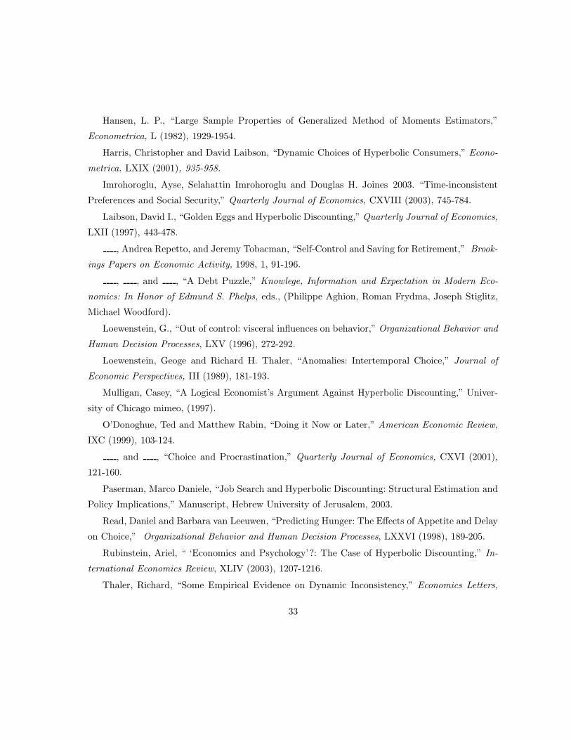
Hansen, L. P., “Large Sample Properties of Generalized Method of Moments Estimators,”

Econometrica, L (1982), 1929-1954.

Harris, Christopher and David Laibson, “Dynamic Choices of Hyperbolic Consumers,” Econo-

metrica. LXIX (2001), 935-958.

Imrohoroglu, Ayse, Selahattin Imrohoroglu and Douglas H. Joines 2003. “Time-inconsistent

Preferences and Social Security,” Quarterly Journal of Economics, CXVIII (2003), 745-784.

Laibson, David I., “Golden Eggs and Hyperbolic Discounting,” Quarterly Journal of Economics,

LXII (1997), 443-478.

, Andrea Repetto, and Jeremy Tobacman, “Self-Control and Saving for Retirement,” Brook-

ings Papers on Economic Activity, 1998, 1, 91-196.

, , and , “A Debt Puzzle,” Knowlege, Information and Expectation in Modern Eco-

nomics: In Honor of Edmund S. Phelps, eds., (Philippe Aghion, Roman Frydma, Joseph Stiglitz,

Michael Woodford).

Loewenstein, G., “Out of control: visceral influences on behavior,” Organizational Behavior and

Human Decision Processes, LXV (1996), 272-292.

Loewenstein, Geoge and Richard H. Thaler, “Anomalies: Intertemporal Choice,” Journal of

Economic Perspectives, III (1989), 181-193.

Mulligan, Casey, “A Logical Economist’s Argument Against Hyperbolic Discounting,” Univer-

sity of Chicago mimeo, (1997).

O’Donoghue, Ted and Matthew Rabin, “Doing it Now or Later,” American Economic Review,

IXC (1999), 103-124.

, and , “Choice and Procrastination,” Quarterly Journal of Economics, CXVI (2001),

121-160.

Paserman, Marco Daniele, “Job Search and Hyperbolic Discounting: Structural Estimation and

Policy Implications,” Manuscript, Hebrew University of Jerusalem, 2003.

Read, Daniel and Barbara van Leeuwen, “Predicting Hunger: The Effects of Appetite and Delay

on Choice,” Organizational Behavior and Human Decision Processes, LXXVI (1998), 189-205.

Rubinstein, Ariel, “ ‘Economics and Psychology’?: The Case of Hyperbolic Discounting,” In-

ternational Economics Review, XLIV (2003), 1207-1216.

Thaler, Richard, “Some Empirical Evidence on Dynamic Inconsistency,” Economics Letters,

33

VIII (1981), 201-207.

34

Table 1: Sample Statisticsa

N Months On Number of Revolving Revolving Number of Income

File Past-due Balance Limit Credit Cards

Allb 599,257 174 0.0197 $2,509 $17,481 3.77 NA

(71) (0.139) (4058) (11388) (1.88)

A 1073 126 0.0308 $3,927 $15,473 3.94 $44,180

(76) (0.1727) (4979) (10573) (2.057) (24051)

B 903 128 0.0266 $3,474 $15,137 3.81 $43,170

(79) (0.1609) (4725) (11112) (2.101) (25175)

C 687 114 0.0247 $3,543 $14,230 3.598 $42,253

(77) (0.1555) (4901) (11268) (2.068) (24437)

D 645 112 0.0248 $3,584 $14,075 3.557 $41,215

(76) (0.1557) (4988) (11703) (2.07) (25274)

E 992 125 0.0363 $3,694 $15,176 3.729 $43,830

(76) (0.1871) (5066) (11313) (2.076) (28733)

F 944 123 0.0222 $4,042 $15,107 3.807 $43,697

(77) (0.1476) (5469) (10688) (1.98) (26725)

aStandard deviations are in parentheses.bSample statistics are reported for all six market cells to save space. Due to randomization, the statistics are

similiar across different market cells.

35

Table 2: Rank Reversala

Market Cell Number of Effective Rank by Effective Rank by

Observations Response Rate Response Rate Interest Rate Interest Rate

A: 4.9% 6 months 99,886 1.073% 1 10.23% 3

(0.00033)

B: 5.9% 6 months 99,872 0.903% 4 11.35% 4

(0.00030)

C: 6.9% 6 months 99,869 0.687% 5 11.86% 5

(0.00026)

D: 7.9% 6 months 99,880 0.645% 6 12.35% 6

(0.00025)

E: 6.9% 9 months 99,890 0.992% 2 9.23% 2

(0.00031)

F: 7.9% b 12 months 99,860 0.944% 3 8.32% 1

(0.00031)

T-TEST P-VALUES

A vs. E 7.23%

A vs. F 0.29%

aStandard errors in parentheses.bIt should be briefly be explained why the calculated effective interest rate for market cell F (8.32%) slightly

exceeded the stated APR of 7.9%. First, the author’s calculations incorporated the first 13 months of the potential

life of the account, in order to deal with some timing problems in the data. Second, the APR is twelve times the

monthly interest rate and, so, omits monthly compounding. Third, the introductory interest rate is conditional on

the card holder remaining current on his account; each market cell includes customers who went delinquent and lost

the introductory rate.

36

0 5 10 15 20 250

500

1000

1500

2000

2500

Market Cell AMarket Cell BMarket Cell CMarket Cell DMarket Cell EMarket Cell F

month

$

Figure 1: Medians of borrowers’ debt distributions over time.

37

0 5 10 15 20 250

0.1

0.2

0.3

0.4

0.5

0.6

0.7

Market Cell AMarket Cell BMarket Cell CMarket Cell DMarket Cell EMarket Cell F

month

frequency

Figure 2: Borrowing Frequencies of respondents over time.

38

0.1 0.2 0.3 0.4 0.5 0.6 0.7 0.8 0.9 10.1

0.2

0.3

0.4

0.5

0.6

0.7

0.8

0.9

1

SophisticatedNaive

β

δ

Figure 3: Rank Reverse Area of Sophisticated and Naive Hyperbolic Agents

39

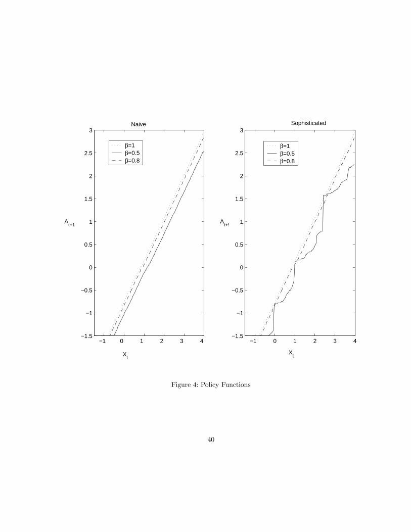
−1 0 1 2 3 4−1.5

−1

−0.5

0

0.5

1

1.5

2

2.5

3

−1 0 1 2 3 4−1.5

−1

−0.5

0

0.5

1

1.5

2

2.5

3Naive Sophisticated

At+1

Xt

At+!

Xt

β=1β=0.5β=0.8

β=1β=0.5β=0.8

Figure 4: Policy Functions

40

−1 0 1 2 3 4 5−1.5

−1

−0.5

0

0.5

1

1.5

2

2.5

3

3.5

4

Naive with β=0.5Sophisticated with β=0.5A

t=A

t+1

At+1

Xt

Figure 5: Policy Functions

41

Table 3: Rank Reversal Response a

Exponential

δ 0.96 0.98 0.99 0.9999

A 152 72 53 41

F 476 100 71 36

Sophisticated

β 0.7 0.8 0.9 0.95

A 98 80 54 47

F 133 72 41 49

Naive

β 0.7 0.8 0.9 0.95

A 133 90 59 47

F 127 91 57 45

aResponse is out of 10,000 simulations. β,δ are discount factors. k, the switching cost parameter, is 0.03. Mean of

A1 is 5000 and variance is 8e6, which is liquid assets at the time of solicitation.

42

1 2 3 4 5 6 7 80

500

1000

1500

2000

2500

3000

3500

Quarter

$

δ=.96δ=0.98δ=0.99δ=0.9999

Figure 6: Simulated Mean Debt among responders of Market Cell A (Exponential)

43

1 2 3 4 5 6 7 80

500

1000

1500

2000

2500

3000

Quarter

$

β=0.7β=0.8β=0.9β=0.95

Figure 7: Simulated Mean Debt among responders of Market Cell A (Sophisticated Hyperbolic)

44

1 2 3 4 5 6 7 80

500

1000

1500

2000

2500

3000

3500

4000

4500

Quarter

$

β=0.7β=0.8β=0.9β=0.95

Figure 8: Simulated Mean Debt among respondents of Market Cell A (Naive Hyperbolic)

45

Table 4: Estimated Parameters a

Sophisticated Naive Exponential

Hyperbolic Hyperbolic

β 0.7863 0.8172

(0.00192) (0.003)

δ 0.9999 0.9999 0.9999

(0.00201) (0.0017) (0.00272)

k 0.02927 0.0326 0.1722

$293 $326 $1, 722

(0.00127) (0.00139) (0.0155)

µ 1.0088 0.9584 1.5836

$5, 044 $4, 792 $7, 918

(0.0367) (0.0277) (0.0517)

ε2 0.831 0.8167 4.278

$8, 310, 000 $8, 167, 000 $42, 780, 000

(0.0439) (0.0373) (0.0535)

Goodness-of-Fit 2.5202e − 4 2.8183e − 4 6.0534e − 4

X2 6110 5627 13975

aβ,δ are discount factors. k is the switching cost parameter. A1 is liquid assets at the time of solicitation. Standard

errors are in parentheses.

46

Table 5: Simulated Response

Market Cell Total Empirical Sophisticated Naive Exponential

Hyperbolic Hyperbolic

A: 4.9% 6 months 99,886 1073 1001 1013 951

B: 5.9% 6 months 99,872 903 888 911 845

C: 6.9% 6 months 99,869 687 793 810 764

D: 7.9% 6 months 99,880 645 652 701 672

E: 6.9% 9 months 99,890 992 980 997 1005

F: 7.9% 12 months 99,860 944 947 978 1047

47

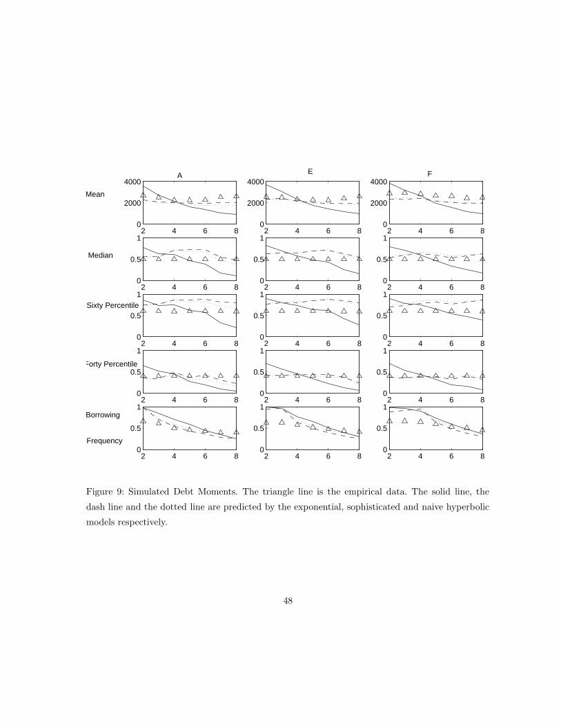
2 4 6 80

2000

4000

2 4 6 80

2000

4000

2 4 6 80

2000

4000

2 4 6 80

0.5

1

2 4 6 80

0.5

1

2 4 6 80

0.5

1

2 4 6 80

0.5

1

2 4 6 80

0.5

1

2 4 6 80

0.5

1

2 4 6 80

0.5

1

2 4 6 80

0.5

1

2 4 6 80

0.5

1

2 4 6 80

0.5

1

2 4 6 80

0.5

1

2 4 6 80

0.5

1

A E F

Mean

Borrowing

Frequency

Median

Sixty Percentile

Forty Percentile

Figure 9: Simulated Debt Moments. The triangle line is the empirical data. The solid line, the

dash line and the dotted line are predicted by the exponential, sophisticated and naive hyperbolic

models respectively.

48

Table 6: Robustness a

Consistent β Sophisticated Naive Exponential

Hyperbolic Hyperbolic

β 0.9999 0.8034 0.8246

(0.002967) (0.00253) (0.00255)

δ 0.9999 0.9998 0.9999 0.9726

(0.002972) (0.00133) (0.00124) (0.000962)

k 0.1722 0.0292 0.03266 0.0825

$1, 722 $292 $326 $825

(0.0115) (0.000945) (0.00129) (0.00358)

µ 1.5836 1.0072 0.9752 1.4534

$7, 918 $5, 036 $4, 876 $7, 267

(0.0422) (0.0305) (0.0346) (0.02997)

ε2 4.278 0.8377 0.8296 2.1854

$42, 780, 000 $8, 377, 000 $8, 296, 000 $21, 854, 000

(0.0437) (0.0393) (0.0514) (0.055)

Goodness-of-Fit 6.04892e − 4 2.50492e − 4 2.63716e − 4 4.90161e − 4

X2 20840 3996 4482 10610

aMarket Cell A is excluded for Sophisticated Hyperbolic, Naive Hyperbolic and Exponential models. β,δ are

discount factors. k is the switching cost parameter. A1 is liquid assets at the time of solicitation. Standard errors are

in parentheses.

49