time-dependent propagation of high … 80-391/p/p jfrcrl-52377 time-dependent propagation of...

SLL 80-391/P/P

JfrCRL-52377

TIME-DEPENDENT PROPAGATION OF HIGH-ENERGY LASER BEAMS THROUGH THE ATMOSPHERE: III

T/P, AO

J. R. Morris

J. A. Fleck, Jr.

December 14, 1977

OJBTBDKmOK STATEMENTX

Work performed under the auspices of the U.S. Department of

Energy by the UCLLL under contract number W-7405-ENG-48.

5S5S22l5""rrf

m

'.ijiy "vWM

» ■ • w t 1,110 WALELY inimaxjj® 4

PLEASE RETURN TO:

BMD TECHNICAL INFORMATION CENTER BALLISTIC MISSILE DEFENSE ORGANIZATION

7100 DEFENSE PENTAGON WASHINGTON D.C. 20301-7100

19980309 389 ÜLWt/

NOTICE

"This report was prepared as an account of work sponsored by the United States Government. Neither the United States nor the United States Department of Energy, nor any of their employees, nor any of their contractors, subcon- tractors, or their employees, makes any warranty, express or implied, or assumes any legal liability or responsibility for the accuracy, completeness or usefulness of any information, apparatus, product or process disclosed, or represents that its use would not infringe privately-owned rights."

NOTICE

Reference to a company or product name does not imply approval or recommendation of the product by the University of California or the U.S. Department of Energy to the exclusion of others that may be suitable.

Printed in the United States of America Available from

National Technical Information Service U.S. Department of Commerce 5285 Port Royal Road Springfield, VA 22161 Price: Printed Copy $ ; Microfiche $3.00

Domestic Domestic Page Range Price Page Range Price

001-025 $ 4.00 326-350 SI 2.00 026-050 4.50 351-375 12.50 051-075 5.25 376-400 13.00 076-100 6.00 401-425 13.25 101-125 6.50 426-450 14.00 126-150 7.25 451-475 14.50 151-175 8.00 476-500 15.00 176-200 9.00 501-525 15.25 201-225 9.25 526-550 15.50 226-250 9.50 551-575 16.25 251-275 10.75 576-600 16.50 276-300 11.00 601-up 1

301-325 11.75

Add $2.50 for each additional 100 Dace inrrt>ment from 601 pages up.

Distribution Category UC-34

IÜ9 LAWRENCE LIVERMORE LABORATORY

University of California/Livermore, California/94550

UCRL-52377

TIME-DEPENDENT PROPAGATION OF HIGH-ENERGY LASER BEAMS

THROUGH THE ATMOSPHERE: III J. R. Morris

J. A. Fleck, Jr.

MS. date: December 14, 1977

CONTENTS

ABSTRACT 1 1. INTRODUCTION 1

t 3-Blooming Model 5 Thin Lens Model 5 Recent Army Studies 5

2. MULTIPLE TIMESTEP*3-BLOOMING MODEL 7 Previous 13-Blooming Studies 7 Description of Model 7 Results of Calculations 9

3. AN EQUIVALENT THIN LENS MODEL FOR THERMAL-BLOOMING COMPENSATION 13 Introduction 13 Basic Equations 14 Return-Wave Conjugate-Phase Correction Algorithm 15 Thin Lens Approximation of Heated Atmospheric Lens and Free-Space Return-Wave Algorithm 16 Numerical Examples 17 Summary and Conclusion 20

4. MODELING LASER PERFORMANCE WITH REALISTIC INTENSITY AND PHASE PROFILES: THE ABEL LASER 20

5. STAGNATION ZONES IN TWO ARMY SCENARIOS 24 Introduction 24 Results 25

Thermal Blooming 25 13-Blooming 26 Jitter and Turbulence 27

A Possible Scaling Law Parameter 28 Summary 28

6. CIRCULAR VS ANNULAR LASER BEAMS 29 7. HIGH-ENERGY LASER BEAM PROPAGATION THROUGH A SMOKE SCREEN .... 31 8. COMPARISON OF PROPAGATION CONDITIONS

AT HELSTF AND NORTH OBSCURA PEAK 34 REFERENCES AND NOTES 38

Preceding PagevBlank

in

TIME-DEPENDENT PROPAGATION OF HIGH-ENERGY LASER BEAMS

THROUGH THE ATMOSPHERE: III

ABSTRACT

An accurate computational model of combined strong t 3-blooming and steady-state multiple-pulse blooming is described. A single-pulse calculation and a series of calculations for an overlap number of 1.5 are presented. A new method is derived for calculating a corrective phase to compensate for thermal blooming. This method, which is based on an equivalent thin lens model, provides a fast and accurate estimate of the compensating phase when most of the phase distortion occurs near the laser. It is capable of computing the steady-state compensation for thermal blooming of either cw or multiple-pulse laser beams in noncoplanar scenarios. Several examples of phase compensation calculations are presented including compensation for a quasi-stagnation zone (an almost zero wind-speed minimum) near the laser. Finally, the effects of realistic intensity and phase profiles, stagnation zones, and smoke clouds on laser beam propagation in Army scenarios are examined. In particular, simulation of the ABEL laser beam with realistic intensity and phase profiles shows that its phase distortion is far more detrimental than its nonideal intensity profile. The stagnation zone calculations suggest that the combination of substantial slewing rates with a small wind speed at the laser will make stagnation zones inconsequential in many Army scenarios.

1. INTRODUCTION

This is the third in a series of annual reports describing the development of computational models of high-energy laser beam propagation through the atmosphere. 1>2 In addition to various coplanar l and noncoplanar2 steady-state algorithms, the first two reports describe digital computer algorithms for calculating the time-dependence of thermal blooming in the isobaric approximation.

An updated list of the features of the computer models—collectively known as the FOUR-D code—is found in Table 1. Four features have been added since Ref. 2:

• Thermal conductivity for use in modeling laboratory scale experiments; • A new multiple time-step t 3-blooming model; • A new predictive phase-compensation method (the Bradley and Herrmann model7 can also be im-

plemented for comparison purposes); and • A simplified method for estimating the long-time average beam spread due to turbulence.

Table 1. Basic outline of current FOUR-D propagation code.

Variables x,y,z,t, where x, y are transverse coordinates and z is axial displacement.

Form of propagation equation Scalar wave equation in parabolic approximation

2ik ^ = Y? S + k2(n2 - 1)& ■ oz L

1

Table 1. (continued)

Method of solving propagation equation

Hydrodynamics for steady-state cw problems

Symmetrized split operator, finite Fourier series, fast Fourier transform (FFT) algorithm

M+l / iAz i\ / z'Az -\ s =«p(-4TVi)«p(-2rx)

(iAz „2\ „«

X = k2 (n2 - 1) .

Uses exact solution to linear hydrodynamic equations. Fourier method for M < 1. Characteristic method for M > 1. Solves

dp 9P,

Transonic slewing

Treatment of stagnation-zone problems for cw beams

v + v — x dx y by

/ bv bV \ po[v

x IT + % W) + VJ-pi = ° '

Steady-state calculation valid for all Mach numbers except M = 1. Code can be used arbitrarily close to M = 1.

Time-dependent isobaric approximation. Transient succession of steady-state density changes; i.e., solves

3P1 9P1 9 0 -+V

X 3 -(^0Cp>VlPl = (7_1) aCf!- bt

Nonsteady treatment of multipulse density changes

Changes in density from previous pulses in train are calculated with isobaric approximation using

3Pl

dt

9P, vx IT ~ WeoCp> VI PX

(7 - l)ac -2 I«» (x,y) 8(t - tn)

Method of calculating density change for individual pulse in train

where Tln(x,y) is «th pulse fluence. Density changes resulting from the same pulse are calculated using acoustic equations and triangular pulse shape.

1) Triangular pulse model for moderate t -blooming:

Takes two-dimensional Fourier transform of

x

where / is Fourier transform of intensity, and T is the time duration of each pulse. Source aperture should be softened when using this code provision.


2) Multiple time-point model for strong t -blooming:

Solves me full set of time-dependent linearized hydrodynamic equations within the pulse. Density is the sum of this solution and steady-state multipulse contribution determined by fluence of current pulse.

Treatment of steady-state multipulse blooming

Previous pulses in train are assumed to be periodic replications of current pulse. Solves

dt x sx y dy 2 - cal \ S(t - tn)

Pulse self-blooming is treated as in the nonsteady-state case.

Treatment of turbulence 1) Uses phase-screen method of Bradley and Brown with Von Karman spectrum. Phase screen determined by

T(x,y) Ldt-1 dky exp [i(kxx + Ay)]

x*(M9*«/2(W> where a is a complex random variable and <t>„ is spectral density of refractive index fluctuations.

2) Alternately, takes the convolution of target-plane intensity with a Gaussian distribution using Lutomirski and Yura's intermediate-range beam-spread formula [See H. T. Yura, Appl. Opt. 10, 2771 (1971)]. The jitter a2 is increased by 0.0242 A;04^ z)1-2 where Cfa is in m~2l3, k in cm-1, and z in cm.

Lens transformation and treatment of lens optics

Compensates for a portion of lens phase front with cylindrical Talanov lens transformation. Uses in spherical case

X =_L + J_ Z/ ZT ZL

where zf is focal length of lens, zT is focal length compensated for by Talanov transformation, and zL is focal length of initial phase front.

Treatment of nondiffraction- limited beams

1) Spherical-aberration phase determined by

XA _ ?£± ,2 . 2,2 0 (x* + y*y

2) phase-screen method of Hogge et al. Phase determined as in turbulence, with

„2;2

* = —r— exp " 2TT V

&)■

where /. is correlation length and a is phase variance.


Adaptive lens transformation

Selection of z-step

Scenario capability

Removes phase

2

N [a.(x. - <x.»2 + 0.(x. - Cx.»l

through lens transformation and deflection of beam. Here X\ = x, X2 = y, averages are intensity weighted, a/ and ßi are calculated to keep the intensity centroid at mesh center, and intensity weighted r.m.s. values of x and y are constant with z .

Adaptive z-step selection based on limiting gradients in nonlinear contribution to phase and limiting the wind-velocity change. Constant z-step over any portion of range also possible.

General noncoplanar scenario geometry capability involving moving laser platform, moving target, and arbitrary wind direction. In coplanar case, wind can be function of z and t.

Treatment of multiline effects Calculates average absorption coefficient based on assumption of identical field distributions for all lines

I a/i e*p(-<yO

f. exp(-az)

Treatment of beam jitter

where f. is fraction of energy in line i at z = 0.

Takes convolution of intensity in target plane with Gaussian distribution:

jitter /jfe-^)

Treatment of predictive phase compensation

X I(x - x', y - y') ,

where o is variance per axis introduced by jitter.

1) Laser beam is propagated a distance z' with steady-state thermal blooming, men back to the laser aperture in vacuuo. Difference between new and original phase is an equivalent thin lens whose conjugate is used to correct for the thermal blooming. Useful when blooming phase change is concentrated near laser. Can be iterated.

2) Bradley and Herrmann scheme is also implemented [Appl. Opt. 13, 331 (1974)]. Useful for coplanar scenarios in which blooming is concentrated near laser.

Code output

Numerical capacity when used with CDC 7600 and restricted to internal memory (large and small core)

Problem zoning features

Isointensity, isodensity, isophase, and spectrum contours. Intensity averaged over contours. Plots of intensity, phase, density, spatial spectrum along specific directions, etc., at specific times.

Plots of peak intensity and average intensity vs time.

Spatial mesh, 64 X 64, 30 sampling times, no restriction on number of axial space increments.

Number of space increments in x and y directions must be equal and expressible as a power of 2.

13-Blooming Model

In Section 2 we describe a new t 3-blooming calculation method. In general three phenomena may require a fully time-dependent calculation: t 3-blooming, transonic slewing, and the occurrence of a null wind velocity. Of these three, only strong t 3-blooming is never amenable to a steady-state analysis. A transonic zone along a slewed laser beam has only a small effect on the beam, 3"5 at least for ranges under 10 km; outside the sonic region, steady-state conditions prevail. Most scenarios do not have a true stagnation point, but rather only a region of low, but finite, transverse wind velocities because the wind velocity rarely lies exactly in the slewing plane. Since the minimum velocity is often an appreciable fraction of 1 m/s for military problems, most military "stagnation zone" problems can be calculated with a noncoplanar steady-state wind field. The calculation of moderate or strong t 3-blooming, on the other hand, requires a time-dependent treatment. 2'6

Since typical multipulse C02 lasers have pulse lengths under 100 /us, interpulse times of over 5 ms, and beam diameters under 1.5 m, the isobaric approximation with a series of impulse source terms adequately describes the air-density change due to all but the current pulse. Finding the density change due to the current pulse requires solving the full set of linearized hydrodynamic equations. 2'6 Within each pulse, the new multiple time-step t 3-blooming method self-consistently solves these equations and the Fresnel wave equation in the presence of an air-density contribution from a periodic replication of the current pulse (multipulse steady- state overlap blooming). This new method, which is based on a Fourier transform, removes the restrictions of our simpler (but faster) trangular-pulse approximation and allows the simulation of pulses whose shape changes drastically in time. It also includes the effect of finite wind velocities within the pulse when v > 0.1 cs

(to our knowledge no other propagation code has included this effect); such effects might be significant when multipulse lasers are used against Mach 0.7 or faster targets in crossing target scenarios.

Thin Lens Model

The extent to which adaptive optics can compensate for thermal blooming is being actively investigated with experiments and computer calculations. 7"9 When the thermal-blooming phase distortion occurs near the laser aperture, several simplified models adequately describe the required phase correction at the laser aperture. For example, Bradley and Herrmann 7 have successfully used a multiple of the line integral of the initial beam shape along the wind direction as the phase compensation for thermal blooming of cw laser beams at moderate to high slewing numbers {Nw = wR/v0 = velocity change/initial velocity) in coplanar scenarios. In Section 3, we describe a more general model of comparable simplicity that computes the phase compensation for steady-state multipulse (when t 3-blooming can be ignored) as well as cw thermal blooming in both coplanar and noncoplanar scenarios. For the case described by Wallace and Pasciak, 8 the latter method gives results comparable with those obtained from a complex ray-trace simulation of an ideal phase-conjugate adaptive optics systems. All of these methods, as well as the work of Brown et al.,9 seem to suggest that the on-target intensity increase due to adaptive optics corrections tends to be modest—a factor of about 2 is typical—even though in some scenarios the improvement can exceed a factor of 6.

Recent Army Studies

Sections 4 to 8 describe a series of thermal blooming studies that are relevant to the Army HEL program. Section 4 compares the performance of large and small aperture systems for the Hughes ABEL laser. It is shown that increasing the aperture size by a factor of 2 significantly improves the performance of the ABEL laser system, especially at long ranges. Section 5 describes the effects of stagnation zones in two typical Army scenarios. For these scenarios, thermal blooming generally reduces the on-target irradiance less than turbulence and jitter. In Section 6, the performance levels of equal-power, equal-outer-diameter, uniformly- illuminated disk and annular laser beams in the cw and high-overlap-number multipulse laser cases are compared; the disk aperture is shown to suffer less thermal blooming in agreement with the results of other groups. 10'n In Section 7, thermal blooming due to a smoke screen located near the laser is discussed. Finally, the results of a study of the relative importance of thermal blooming at two potential White Sands Missile Range laser test sites are described in Section 8.

o

ziuo//wi/\l - Ajjsu8;u|

E o

en 3

TJ CO

DC

S

oxi .5 B

ZW3/MIAI - Ansuajui

1 E H

2. MULTIPLE TIMESTEP 13-BLOOMING MODEL

Previous f3-Blooming Studies

Both computational2'6 and experimental n studies of strong t 3-blooming in a stationary absorbing atmosphere indicate that initially bell-shaped irradiance profiles develop a deep on-axis depression late in the pulse. A typical result2 for a square-temporal pulse and a Gaussian beam is shown in Fig. 1. At the successively later times, the pulse shape flattens and broadens, ultimately developing a deep central depression with a high-intensity rim. At even later times, the rim itself actually splits and broadens. Figure 2 shows the saturation of the on-axis fluence due to the central depression in the back of the pulse. When / 3-blooming is severe, no steady-state model that ignores this intrapulse time-dependence can adequately simulate the ther-

mal blooming. Our previous investigations l<2 have shown that a simple single-time-step triangular-pulse model ade-

quately describes 13-blooming prior to significant saturation of the on-axis fluence. The computational speed gained by using only a single timestep makes this model extremely attractive when it is applicable. However, it oversimplifies the physics of strong t 3-blooming by assuming a fluence approximately proportional to the intensity at the center of the pulse. .

The perturbation theory expressions currently in use 13'14 are even more drastic oversimplifications of the physics of strong t 3-blooming when overlap-blooming is significant. They are based on the assumption that the / 3-blooming is driven by the unbloomed laser beam shape, consequently they overestimate t ^-blooming by ignoring the increased laser beam spot sizes near the target due to phase changes induced by overlap- blooming near the laser. Even if overlap-blooming is negligible, the perturbation expressions tend to un- derestimate the time required for the on-axis fluence to saturate by ignoring the self-moderating negative feed- back of self-consistent t 3-blooming. Nonetheless, the perturbation expressions provide useful estimates for t 3-blooming irradiance reductions, if overlap-blooming is negligible.

Description of Model

Within a representative pulse, the FOUR-D code's new multiple time-step t 3-blooming routine self- consistently solves the full set of time-dependent linearized hydrodynamic equations and the Fresnel wave

equation:

2ik £ &(T,t) + Vx &('.')

+ —7 ^ 6p(r,0 &(r,0 = 0

_D Dt

D

Pl(r,0 + \!/(r,f) = 0 ,

^ *(r,0 + VT Pl (r,r) = 0 Dt

(1)

(2a)

(2b)

^ [Pl(r,0 - c2 Pl(r,0] = 5(r,0 , (2c)

20 40

Time — MS

60 80

with

Figure 2. Saturation of the on-axis fluence for the strong t - blooming case of Fig. 1. The circles are the results of the triangular pulse t -blooming model.

Sp(r,0 = (7 - 1) I /-I

F(r - / vnAO Pi (r) .

^ = P0 Vx • Vj (r,f)

5 = (7 - 1) a /(r/),

D - 9 4. T7 DT

= aF +vo • vi

where 8p is the total perturbation in the air density including the effects of heating by previous pulses; p0 is the ambient air density; v0 is the transverse wind velocity relative to the laser beam; ph vj, and/?! are, respectively, the density, the local flow velocity, and pressure changes due to the current pulse; / is the instantaneous intensity of the laser beam; F is the single-pulse fluence; <T is the slowly varying complex electric field amplitude; At is the time between pulses; and the remaining quantities have their usual physical significance. The density term that contains F is the multipulse steady-state contribution to the air density in which all pulses are assumed to be identical. Equations (2) are solved with z as a parameter, since the laser beam changes shape only over distances that are large in comparison with its diameter.

The split-step finite Fourier method of solving Eq. (1) reduces the calculation to alternate free- propagation and phase-screen steps. The latter uses the density 6p calculated from the instantaneous intensity and the single-pulse fluence at the location of the phase screen. Equation (2a) can be used to eliminate p \ from Eq. (2c); this reduces Eqs. (2b) and (2c) to a coupled pair of equations in the variables px and \p. After these equations are Fourier transformed in the spatial variables x and y, they are diagonalized by changing the variables:

*+(k,,0 = 4± * w (4)

These variables, then, satisfy

3 ~ ~ ~ SQuj) ä7 *± + *± ' vo^± ± icsK^± = —~ (5)

Since? is a known function of?, the solution of Eq. (5)for/„+1 < t < t„ is given by:

P±(kx,ky,t) = exp (-«7±fH ?± On) exP (*?± iq+Jn) + I dt'l

t ~ jSi^t'))

exp (iq+t') (6)

J

where q+ = k • v„ ± c |k±| . The value of S can be approximated by

S(kvt) = afij (t - tn) + \{\) for tn + 1 > t> tn.

Then, <i>± at the next time step is given by

Xn+l n, \ - 'Xß C (ki) = ™± exp (-iq±At) +c; ■fart-K)

X q-±l • 2i sin(^q± At) exp (-- iqt Af) - ianAtq±

lV . (7)

After 0+ and </>_ are obtained from Eq. (6), px can be obtained from Eqs. (4) and the density p {is given by the solution of Eq. (2c):

pfl = \ [?J+1 + r_+1] + "< [ Ti - j(?+" + ?-")] «P (~t\ • v0 AO

^iLi /'n + l

or more explicitly by

p«+l - [p* - I (?* + ^)]exP (WVQAO + ^(?+"+1 + ?-"+1)

a c-2 n s [2/ (Vo'k^-2 sin(|v0 • k±A/) exp (- ±- nr„ • l^Af) -z(vQ • kj"1 A?]

- 5, *;2 [2 <vo * ki)_1 sin (j v0 * ki At) exP (" 5" zVo * ki At)] •

(8)

(9)

Equations (7) and (9) mathematically describe the intrapulse density update. Three arrays corresponding to T>\,]f\, and ^must be carried from timestep to timestep (the latter two to provide values of ^±).

Previous numerical solutions 2'6 of strong t 3-blooming have ignored the wind velocity within the pulse. If the effective wind velocities near the target exceed Mach 0.7, intrapulse wind velocity effects will be significant (if? 3-blooming is important at all). The reason is illustrated in Fig. 3 for a Mach-1.5 wind across a Gaussian laser beam. The density profile is no longer centered on the laser-beam axis (located at the +), but is forced downwind. After a sound transit time, it begins to develop the Mach stem that characterizes the steady-state density profile. Its shape does not even vaguely resemble the V2/ profile that is characteristic of zero wind velocity.

Results of Calculations As a test of the FOUR-D code's new multiple timestep t 3-blooming model, the single-pulse calculations

of Figs. 1 and 2 for 1.8-km range were repeated. The initial laser beam was assumed to have an infinite Gaus- sian shape with a 50-cm e ~2 intensity diameter. The beam was focused at 2.5 km. The temporal pulse shape

Time — /is

Figure 3. Evolution of heated air-density profiles in a Mach-1.5 wind. The scale lines are cs t, where cs is the speed of sound. The heat source is a Gaussian laser beam.

was assumed to be square, with a 133-yus duration, and the pulse energy was assumed to be 62 kJ. The laser wavelength was 10.59 ^m, and the atmospheric-absorption coefficient was assumed to be 0.3 km ~K The beam quality was 2 times diffraction-limited, represented by wavelength-scaling throughout. The results are shown in Fig. 4. For approximately the first 10/ts, the beam profile remains nearly Gaussian as the heated air has not yet had time to expand and create a significant density change. By 33.3 ßS, the density change along the laser beam has become significant and the laser intensity profile is noticeably more flat-topped than the initial Gaussian. By 66.6 ßs, the intensity has a pronounced on-axis depression and a shape like a doughnut. At 100/is, the central depression has become deeper and the doughnut radius has expanded. By 133.3 jus, the doughnut rim itself has widened and developed its own central depression. The maximum intensity vs time for this same calculation (Fig. 5) decreases steeply until the depression develops, plateaus as the rim merely ex- pands, and then drops again as the rim is bloomed. Qualitative agreement of the present model with the results

10

-0.1 0 0.1 -0.1 0 0.1 -0.1 0 0.1 -0.2 -0.1 0 0.1 0.2 -0.3 -0.2 -0.1 0 0.1 0.2 0.3

6.7 33.3 66.7 100 133.3

Time — /xs

Figure 4. Single-pulse (t3-) blooming in the Four-D code. Time-dependence of the radial intensity profiles under strong f3 -blooming condi-

tions.

20 40 60 80 Time — ßs

100 120 Figure 5. Time-dependence of the maximum intensity for the calculation of Fig. 4. The upper flat curve is the unbloomed intensity.

of the previous detailed radially-dependent code is obvious; the quantative agreement is satisfactory also. The FOUR-D code customarily uses less computer time than the radially-dependent code. It is also generally simpler to use because of its adaptive lens transformation, and it can perform a much wider class of thermal- blooming calculations because it is not restricted to radially symmetric problems.

11

Figure 6 illustrates combined overlap- and t 3-blooming when N0 = 1.5, ND =319, and NF = 29.6. A laser beam with 2.0-MW power, 15-Hz rep. rate, and a 1-m truncated Gaussian profile was simulated; it was focused at 3 km and the target was at 2.5 km. At 6.7 and 13.3 us, only overlap-blooming is significant; by 20 ßs, strong t 3-blooming is evident. Strong t 3-blooming distortion at and beyond 20 ßs does not seem to alter the overlap-blooming much, as can be seen from the similarity of the overlap-only irradiance and the 6.7- ßs irradiance. This might form the basis of a simple scaling law for 13-blooming, in which the overlap- blooming is estimated first and t 3-blooming is estimated using the overlap-bloomed laser beam area.

Near-vacuum values of the on-target peak time-averaged intensity were obtained in spite of the large distortion number. In the calculation without t 3-blooming, this intensity was 38% larger than the 11.4-kW/cm 2

on-target peak time-averaged intensity of the same beam propagated through a vacuum but corrected for the linear absorption power loss; this focusing effect when the overlap number is between 1 and 2 has been noted before. 2 With t 3-blooming included, the on-target peak time-averaged intensity is 72% of the vacuum value.

6.7 13.3 20.0 26.7

Time — ps

Overlap-blooming only Time-averaged intensity

Figure 6. Time-dependence of on-target irradiance for strong t -blooming combined with overlap blooming at yv0 = 1.5.

12

The t 3-blooming also forces the instantaneous intensity centroid of the laser beam to successively farther upwind positions- 3.1, 3.3, 5.8, and 7.5 cm at successive time increments of 6-2/3 fis. Because the growth of the density change during a pulse is due to the propagation of a sound wave driven by the laser heating of the air, the density change lags behind the laser heating. The shape of the laser beam at early times is the dominant factor in determining the density seen by the laser beam at late times. This lag probably explains the motion of

the intensity centroid during the pulse. .„._„, The power-dependence of the combined overlap- plus t 3-blooming for this case is shown in Fig. 7. Ine

overlap number, repetition rate, and initial peak intensity were held fixed, and only the pulse length was varied For this method of power adjustment, overlap-blooming increases the diffraction-limited intensity more than t 3-blooming reduced it, until the power exceeds 860 kW. Above 860 kW, t 3-blooming dominates and the on-target intensity is saturated. Note, however, that this calculation used a particularly favorable overlap number—one leading to a weak focusing (plus deflection) of the laser beam.

Varying the power by changing the repetition rate while maintaining the peak intensity and using the 26.7-/is pulse length (the 2-MW pulse length in our calculations) would change the results in Fig. 6 in the

following ways: . ,..,,, . . ,■ u • The curve without t 3-blooming would follow the linear diffraction-limited behavior up to higher

power levels, joining the present curve at 2 MW. It would, thus have a larger slope at 2 MW • The fractional decrease in the on-target intensity due to 13-blooming would be at least as large at all

lower power levels as it is at 2 MW in our calculation, since the pulse energy and pulse duration upon which t 3-blooming depends would then be constant. The two curves would remain separate down to the lowest

usable power. ,„„»,„,, ? i j *u <■ Because the on-target peak intensity at the 1-MW power level exceeded 20 MW/cm 2, we conclude that,

for overlap numbers of 1.5 or less and pulse lengths under 100 Ms, the propagation of 1-m-optics C02 laser beams out to ranges exceeding 2.5 km will be limited primarily by the dirty air breakdown threshold, rather than by thermal blooming. Multipulse C02 laser beams with multimegawatt power levels will have to be focused beyond the target to avoid breakdown during the first few microseconds of the pulse.

CD OS

E CM S> E

k 5 T3 ■C

CO

I CD Ü to D.

C/3

V) C CD

10 I r

Without f3-blooming

Diffraction

/ With f3-blooming

0.5 1.0 1.5 2.0

Power - MW

2.5 Figure 7. Average on-target intensity vs input power. The power was varied by altering the pulse length while keeping all other parameters constant.

3. AN EQUIVALENT THIN LENS MODEL FOR THERMAL-BLOOMING COMPENSATION

Introduction

Several optical techniques have been investigated for reducing the distortion of high-energy laser beams propagated through the atmosphere. These include coherent optical adaptive techniques (COAT), which are

13

based on receiving a phase front in the transmitter aperture from an unresolved spot (glint) on the target. Two experimental forms of COAT have been investigated. The first of these is the phase-conjugate COAT System, 16>17 wherein the phase from the glint is measured by interferometric means, and the conjugate of this phase is in turn applied as a correction to a phased array of mirrors. The system is adaptive in that the monitoring of the return wave and the adjustment of the phased array are carried out continuously. A second COAT system is the multidither scheme, 18 which relies on a dithering or modulation of the elements of the phased array to maximize the intensity of the glint return. The performance of both the phase-conjugate and the multidither systems, including the finite resolution of both the adaptive mirror and the phase sensor array, has been simulated by Brown. 19

It is also possible to determine a phase correction by a purely predictive method that depends only on a knowledge of the relevant atmospheric parameters and does not require measured information from a target- glint return. Since the two COAT systems are adaptive, they can in principle correct for both thermal blooming and atmospheric turbulence. Predictive methods, on the other hand, are restricted to thermal-blooming compensation, since the relevant detailed information on atmospheric turbulence is never available.

A predictive phase-correction method applicable to cw thermal blooming was first demonstrated by Bradley and Hermann. 7 This method assumes the phase correction to be proportional to the thermally- induced density change at the transmitter. The constant of proportionality is initially estimated by integrating the reciprocal of the wind speed along the propagation path, but it is finally adjusted by iteration. This method works well when the atmospheric heating is concentrated near the aperture, but it works better for cw beams than for multipulse beams. This is apparently due to the fact that the density variation with propagation distance cannot be extrapolated as easily for multipulse beams as it can for cw beams.

A second predictive scheme applicable to multipulse laser beams is due to Wallace and Pasciak. 8 This method determines the conjugate-phase correction by following ray trajectories from a point source in the focal plane back through the heated medium to the transmitter in a geometric optics approximation. The method also utilizes the time development of the thermal blooming to calculate the phase correction and the atmospheric heating self-consistently. This can be done because the thermal blooming for a given pulse depends solely on the atmospheric heating by previous pulses and can thus be considered a strictly linear effect.

In this report we describe a new predictive technique that is based on a thin lens approximation of thermal blooming. It compares favorably in accuracy with the two previously mentioned methods. It also has some practical advantages, including ease of application and versatility. It represents a generalization of the earlier Bradley-Herrmann scheme in that it can employ information on the density distribution along the entire propagation path if necessary. At the same time it avoids some of the complications that can occur in the modeling of phase-conjugate systems. It is equally applicable to cw and multipulse beams and can be expected to work well whenever the effective atmospheric lens is concentrated near the transmitter, a condition that seems to be necessary for the unqualified success of any COAT or predictive phase-correction scheme. In some marginal cases, the method may give useful corrections if only a portion of the atmospheric lens near the aperture is compensated.

Because of its simplicity—determination of a phase correction requires only the computation of the Fourier transform of a propagated field—the method is readily applicable with adaptive coordinate transfor- mations and noncoplanar geometry, which are required for many practical analyses. Noncoplanar geometry is particularly useful for studying the effects of stagnation zones. 1>20 All real-world scenarios are in some measure noncoplanar, and noncoplanarity provides a nonvanishing vertical transverse wind component within the stagnation zone that allows a greatly simplified steady-state analysis. 2

The remainder of Section 3 begins with a review of basic equations. Subsequently, a wave-optics method for computing a return-wave conjugate-phase correction is derived; however, no further use is made of this model. Thereafter, the thin lens representation of thermal blooming is described and used to derive a simpler phase-correction method. Finally, the second method is compared with the methods of Refs. 7 and 8 in sam- ple calculations. Results for a representative scenario involving a stagnation zone are also given.

Basic Equations

The electric field amplitude & is assumed to satisfy the Helmholtz equation in Fresnel approximation

2ik^ = vH +k28e& , (10) oz 1

14

where the intensity / is given in terms of & and the absorption coefficient a by / = | & | 2 exp(-az), Vf = 3 2/8* 2

+ 8 2/dy 2 is the transverse Laplacian, and 8e = (be/dp)5p is the hydrodynamically-induced change in permit- tivity. The steady-state density change for cw beams satisfies

, 95£ + v M£ = _!l_IlJl (11) * bx y by „2

Ls

The corresponding steady-state density change for multipulse beams, on the other hand, is governed by the equation

!fr + ;*£+>,%--1T-™°' I «'-'■> (12)

which is based on the steady-state assumption that all pulses in the train have the same spatial intensity distribution for a given value of z. In the most general case of a noncoplanar scenario the transverse wind velocity vector v = (yx,vy) rotates in the transverse plane, and the velocity components vjz) and are vy(z) linear func- tions of z. Methods for solving Eqs. (11) and (12) are described in Ref. 2.

The numerical solution for the field & T in the target plane can be expressed formally in terms of the field &° in the aperture plane by means of the equation

where the Hermitian operator &NL is defined by *

*« - n «P& V?) exp(f «A) «xp(^i vj) • Ofl

Application of &NL is most easily carried out in terms of Fourier transforms, but it is, in any case, equivalent to a sequence of free-space propagation steps through free space alternating with the imposition of the phase fronts <p = -(k/2) Se} Azj; where Se is an average of 5e over the path AZJ, and the free-space propagation is governed by

2ft |* - Vl * • <15> oz x

Return-Wave Conjugate-Phase Correction Algorithm

A wave-optics analog of the conjugate-phase method of Ref. 8 can be derived with the help of Eqs. (13) and (14). We wish to determine a function \p(x,y) such that

9NL^& = V • (16)

where &L is the operator that propagates a field from the transmitter to the target through free space, i.e.,

15

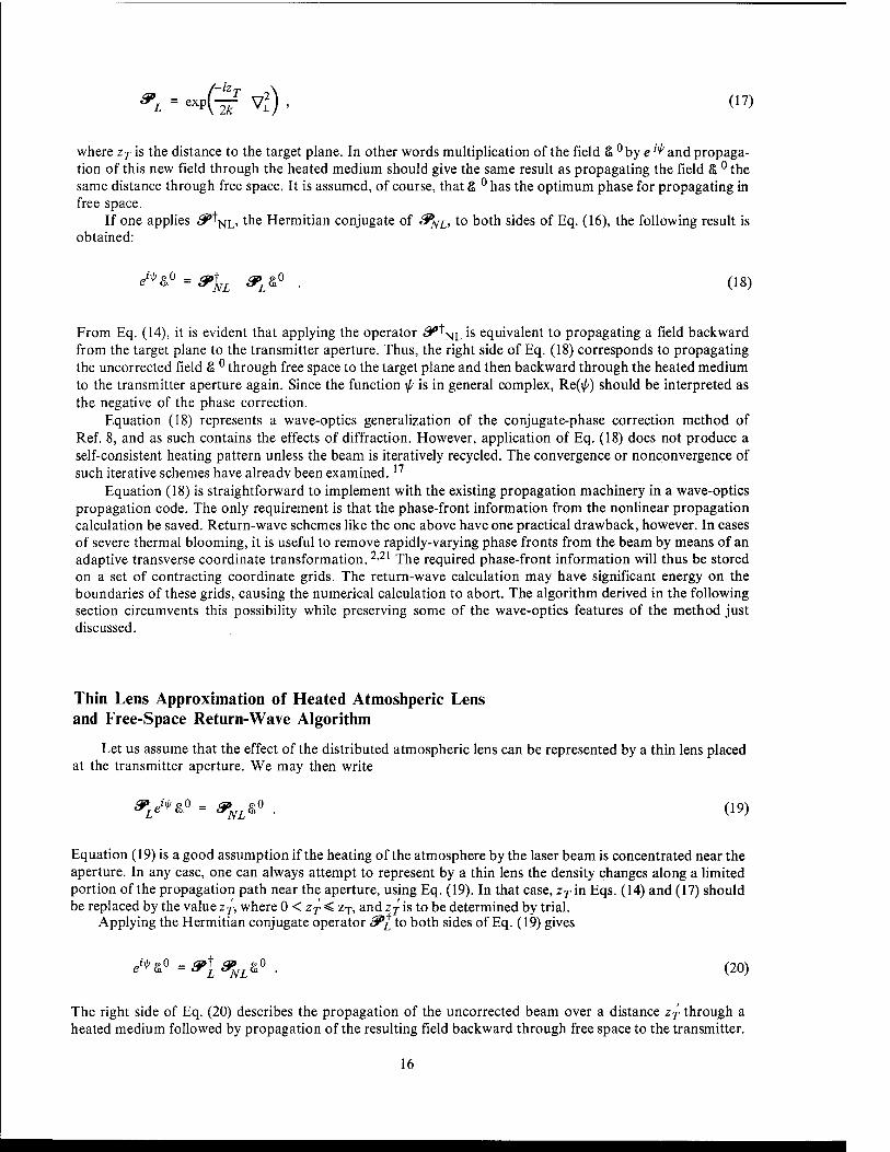
& L

eXp(i? V,2) , (17)

where zT is the distance to the target plane. In other words multiplication of the field £ ° by e "^ and propagation of this new field through the heated medium should give the same result as propagating the field £ ° the same distance through free space. It is assumed, of course, that £ ° has the optimum phase for propagating in free space.

If one applies <^NL> tne Hermitian conjugate of &>NL, to both sides of Eq. (16), the following result is

obtained:

e^&° = &\L &L&° . (18)

From Eq. (14), it is evident that applying the operator <^NL is equivalent to propagating a field backward from the target plane to the transmitter aperture. Thus, the right side of Eq. (18) corresponds to propagating the uncorrected field £ ° through free space to the target plane and then backward through the heated medium to the transmitter aperture again. Since the function \p is in general complex, Re(iZ') should be interpreted as the negative of the phase correction.

Equation (18) represents a wave-optics generalization of the conjugate-phase correction method of Ref. 8, and as such contains the effects of diffraction. However, application of Eq. (18) does not produce a self-consistent heating pattern unless the beam is iteratively recycled. The convergence or nonconvergence of such iterative schemes have already been examined. 17

Equation (18) is straightforward to implement with the existing propagation machinery in a wave-optics propagation code. The only requirement is that the phase-front information from the nonlinear propagation calculation be saved. Return-wave schemes like the one above have one practical drawback, however. In cases of severe thermal blooming, it is useful to remove rapidly-varying phase fronts from the beam by means of an adaptive transverse coordinate transformation.2'21 The required phase-front information will thus be stored on a set of contracting coordinate grids. The return-wave calculation may have significant energy on the boundaries of these grids, causing the numerical calculation to abort. The algorithm derived in the following section circumvents this possibility while preserving some of the wave-optics features of the method just discussed.

Thin Lens Approximation of Heated Atmoshperic Lens and Free-Space Return-Wave Algorithm

Let us assume that the effect of the distributed atmospheric lens can be represented by a thin lens placed at the transmitter aperture. We may then write

05V*&° = &NL&° . (19)

Equation (19) is a good assumption if the heating of the atmosphere by the laser beam is concentrated near the aperture. In any case, one can always attempt to represent by a thin lens the density changes along a limited portion of the propagation path near the aperture, using Eq. (19). In that case, zrin Eqs. (14) and (17) should be replaced by the value zj, where 0 < zj < zT, and zj is to be determined by trial.

Applying the Hermitian conjugate operator &*[ to both sides of Eq. (19) gives

j*&° =&l &NL&° . (20)

The right side of Eq. (20) describes the propagation of the uncorrected beam over a distance zj through a heated medium followed by propagation of the resulting field backward through free space to the transmitter.

16

Computation of \p thus requires a single Fourier transform and no storage of phase fronts. Since a thermally- bloomed beam is larger than the corresponding diffraction-limited beam, the return beam is usually smaller than the original uncorrected beam and easily fits inside the aperture grid. Determination of a best correction requires varying the parameter zT. When the optimum value of zj has been determined, an improved correction may be obtainable by iterating to find a self-consistent heating distribution. However, experience has shown that such additional iterations usually result in only marginal improvement.

Numerical Examples

The first numerical example has been treated in Ref. 7. The pertinent data are

NE

NA

= ka2/R = 18.3

= aR = 0.4

N = CJä/V0 =

ND = IJL 1 (?)(£) (?)-"»

where NF = Fresnel number, NA = absorption number, Na = slewing number, and ND = distortion number. Here a is the 1 /e-radius of a Gaussian beam that has been truncated at its 1 /e 2-radius, and the range R - zT is taken equal to the initial radius of curvature of the beam zf. The isointensity-contour plots for the corrected and the uncorrected beam are displayed in Figs. 8a and 8b. The correction was based on Eq. (20). A phase correction A<t> based on the method of Ref. 7 was also calculated:

A<t> = -ya2ND

2N P ln(l + *«> /

-'_oo

|&(z = 0,x',y)\2 dx (21)

Computations based on the two phase correction methods are compared in Table 2. In Table 2 the intensities have been averaged over the isointensity contour containing one-half the beam

power. The value of y in Eq. (21) and the ratio zT/R have been optimized to yield the maximum value of

Figure 8. Isointensity contours for cw beam in focal plane. Con- tours decrease from peak value in increments of 0.1. Problem parameters are NF = 18.3, NA = 0.4, Nu = S,ND = 107; (a) uncorrected beam, (b) corrected beam using Eq. (11) and zj/R = 0.5. Correction decreases half-power area by a factor of 2.

Table 2. and Eq.

Comparison of results (21).

using Eq. (20)

Eq. (20) Eq. (21)

/ 11° *AV AV 2.09 1.78

7 - 1.0

Z'JJR 0.5 -

17

1AVIIAV< where I%v is the average intensity for the uncorrected beam. The optimum value of IAV/I%V for

Eq. (20) is about 17% larger than the corresponding value for Eq. (21). Further improvement in the correction resulting from Eq. (21) can be obtained by readjusting the focal position zf. The same presumably holds true for Eq. (20). However, no attempt has been made to apply a refocusing correction here.

The second illustrative example is taken from Ref. 8 and deals with a multipulse beam. The relevant parameters are

N0 = 2a/v0A; = 4

^„ = 0

NF = 9.08

NA = 0.4

ND = 17.9

where N0 is the overlap number. The beam is assumed to be an infinite Gaussian with l/e 2 radius equal to a. The uncorrected and corrected steady-state isointensity profiles at the target are shown in Figs. 9a and

9b. The uncorrected peak intensity is 0.52 times the value for the diffraction-limited beam. Following the correction based on Eq. (20), the peak intensity is 0.95 times the diffraction-limited value, in essential agreement with the result in Ref. 8. For this example the optimum value of zj/R was equal to 1. An additional iteration resulted in inconsequential improvement.

The final example involves a cw beam propagating through a noncoplanar stagnation zone. The horizontal wind speed as a function of axial distance is seen in Fig. 10a, and the velocity magnitude as a function of z is shown in Fig. 10b. The stagnation point (position of vanishing of horizontal component of wind velocity) is located 75 m from the aperture. The defining parameters for the problem are the following:

NA = 0.183

NF = 86.7

ND{Q) = 450

NDizD) = 851

NJZD) _ \v(R)\

WzD)\

V,(Zn) = 0.727 m/s

81.8

Figure 9. Isointensity contours for multipulse beam in focal plane. Problem parameters are N F = 9.08, NA = 0.4, Nw = 0, ND = 18.6. Initial beam shape is Gaussian; (a) uncorrected beam, (b) beam corrected using Eq. (11) and z 'T/R = 1. For the uncorrected beam the peak intensity is 0.53 times the peak for a diffraction- limited beam. Following correction this rises to 0.95 times the diffraction-limited peak.

18

The beam at z = 0 is a uniformly-illuminated circular aperture, and the slewing number refers to the stagnation point z = zD. The distortion numbers are calculated at both the aperture and the stagnation point, where v^, the vertical component of wind velocity in the transverse plane, is substituted for VQ. The distortion and slew numbers are given only to characterize the problem. Due to the complexity of flow in the stagnation zone, these numbers cannot be used to infer the thermal-blooming characteristics from those of a coplanar scenario with similar values.

The uncorrected and corrected isointensity contours in the target plane are shown in Figs. 1 la and 1 lb, and the isophase contours for the corrective phase that must be applied on the aperture mirror are shown in Fig. 12.

The areas of the uncorrected beam, the corrected beam, and a diffraction-limited beam in the target plane are compared in Table 3. The area used is that of the isointensity contour containing half of the beam power. Although the thermal blooming is clearly severe, Table 3 indicates that a phase correction can give an improvement by a factor of about 2 in the average intensity. This example suggests that phase compensation for thermal blooming can be of some use in stagnation-zone situations, if the stagnation zone is situated near the aperture.

E I

■4-" c <D C o Q. E o u

u _o > -a c

c o N

o X

0 I i l | i I i i | I I 1 I |

10 (a)

—

20 —

30 —

40 v —

50 i i i 1 , , , , 1 , iiil

1 2

Axial distance — km

1 2

Axial distance — km

Figure 10. Transverse wind velocity as a function of axial distance for noncoplanar scenario involving a stagnation zone. (a) Horizontal component vanishes 75 m from aperture, (b) Transverse velocity magnitude does not vanish at stagnation point due to 0.727-m/s vertical component.

Figure 11. Isointensity contours at focus for stagnation zone scenario: (a) uncorrected, (b) corrected. Correction increases average intensity by factor of 2.

19

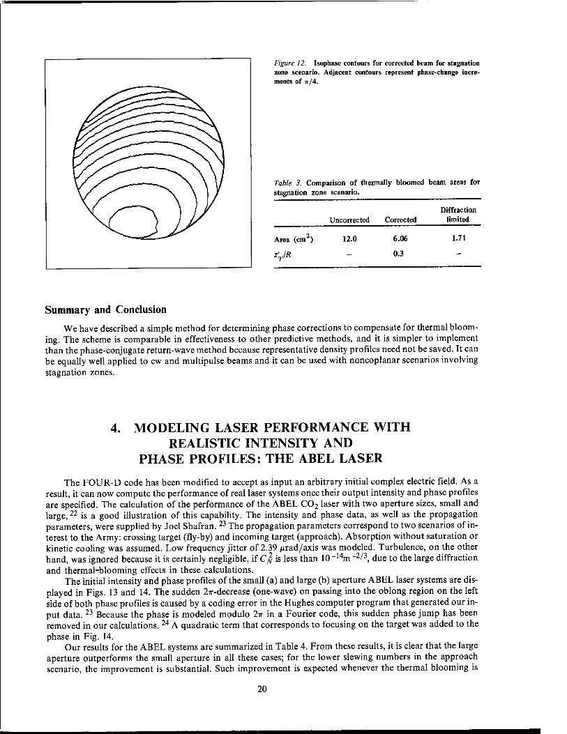
Figure 12. Isophase contours for corrected beam for stagnation zone scenario. Adjacent contours represent phase-change increments of 7r/4.

Table 3. Comparison of thermally bloomed stagnation zone scenario.

beam areas for

Unconected Corrected Diffraction

limited

Area (cm2) 12.0

fjJR

6.06

0.3

1.71

Summary and Conclusion

We have described a simple method for determining phase corrections to compensate for thermal blooming. The scheme is comparable in effectiveness to other predictive methods, and it is simpler to implement than the phase-conjugate return-wave method because representative density profiles need not be saved. It can be equally well applied to cw and multipulse beams and it can be used with noncoplanar scenarios involving stagnation zones.

4. MODELING LASER PERFORMANCE WITH REALISTIC INTENSITY AND

PHASE PROFILES: THE ABEL LASER

The FOUR-D code has been modified to accept as input an arbitrary initial complex electric field. As a result, it can now compute the performance of real laser systems once their output intensity and phase profiles are specified. The calculation of the performance of the ABEL C02 laser with two aperture sizes, small and large,22 is a good illustration of this capability. The intensity and phase data, as well as the propagation parameters, were supplied by Joel Shafran. 23 The propagation parameters correspond to two scenarios of interest to the Army: crossing target (fly-by) and incoming target (approach). Absorption without saturation or kinetic cooling was assumed. Low frequency jitter of 2.39 ^trad/axis was modeled. Turbulence, on the other hand, was ignored because it is certainly negligible, if C^ is less than 10 _14m "2/3, due to the large diffraction and thermal-blooming effects in these calculations.

The initial intensity and phase profiles of the small (a) and large (b) aperture ABEL laser systems are displayed in Figs. 13 and 14. The sudden 27r-decrease (one-wave) on passing into the oblong region on the left side of both phase profiles is caused by a coding error in the Hughes computer program that generated our input data. 23 Because the phase is modeled modulo 2ir in a Fourier code, this sudden phase jump has been removed in our calculations. 24 A quadratic term that corresponds to focusing on the target was added to the phase in Fig. 14.

Our results for the ABEL systems are summarized in Table 4. From these results, it is clear that the large aperture outperforms the small aperture in all these cases; for the lower slewing numbers in the approach scenario, the improvement is substantial. Such improvement is expected whenever the thermal blooming is

20

(a) (b)

Figure 13. Isointensity contours at the laser aperture: (a) small diameter system, (b) large diameter system.

(a) (b)

Figure 14. Isophase contours at the laser aperture: (a) small diameter system, (b) large diameter system. The contour interval is TT/4 (X/8).

21

Table 4. Relative performance of the small and large aperture ABEL laser systems.

Aperture and

Fresnel No.

Absorption No. Distortion Slewing Overlap

Normalized on -target areas

scenario* (NF) (NA) No. No. No. Without jitter With jitter

Small, XT 24.2 0.45 825 301 87.5 12.4 14.3

Large, XT 111.1 0.45 415 301 188.0 9.8 11.2

Small, IT 72.6 0.15 275 91 87.5 1.5 1.7

Large, IT 333.4 0.15 138 91 188.0 = 1.0 1.2

Small, ITC 24.2 0.45 825 31 87.5 107.0 107.0

Small, IT 24.2 0.45 412 16 43.8 43.0 48.0

Large, IT 111.1 0.45 415 31 188.0 14.7 17.3

aXT = crossing target flying into wind. IT = incoming target, 0.1 X (XT range) offset, laser-slewed into wind. Smallest area that contains half the power.

'Marginal calculation, probably overestimates thermal blooming.

large and the overlap number for the smaller aperture is larger than 2 (in these calculations, the overlap number at the laser aperture is 87.5 for the small aperture). Figures 15 to 17 are the on-target irradiances. In the crossing-target scenario (Fig 15) the on-target irradiance has a well-defined central peak with a broad wing that is more elongated along the direction perpendicular to the wind than parallel to it, and the small aperture case has considerably more substructure in the form of secondary peaks than does the large aperture. The on- target irradiance profiles at the shortest range in the incoming-target scenario (Fig. 16) are almost identical to the corresponding crossing-target profiles (Fig. 15), except for a scale factor; the intensities are about 10 times larger and the spot diameter is about 0.4 as large. At the longest range in the incoming-target scenario, a long ridge structure is the most prominent feature of the irradiance profiles. This elongation perpendicular to the direction of the wind will probably become even more pronounced at the longer ranges due to the transverse defocusing action of the nearly stagnant air near the laser aperture, where the laser beam is roughly circularly symmetric.

(a) (b)

Figure 15. On-target isointensity contours for the crossing target scenario: (a) small diameter system, (b) large diameter system. The reference lines represent equal lengths.

22

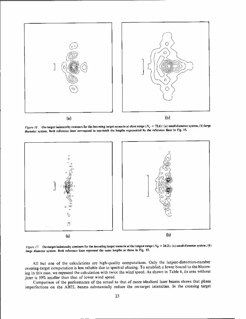
(a) (b)

Figure 16. On-target isointensity contours for the incoming target scenario at close range (NF = 72.6): (a) small diameter system, (b) large diameter system. Both reference lines correspond to one-tenth the lengths represented by the reference lines in Fig. 15.

(a) (b)

Figure 17. On-target isointensity contours for the incoming target scenario at the longest range (WF = 24.2): (a) small diameter system, (b) large diameter system. Both reference lines represent the same lengths as those in Fig. 15.

All but one of the calculations are high-quality computations. Only the largest-distortion-number crossing-target computation is less reliable due to spectral aliasing. To establish a lower bound to the blooming in this case, we repeated the calculation with twice the wind speed. As shown in Table 4, its area without jitter is 59% smaller than that of lower wind speed.

Comparison of the performance of the actual to that of more idealized laser beams shows that phase imperfections on the ABEL beams substantially reduce the on-target intensities. In the crossing target

23

scenario where the thermal blooming is smallest, replacing the actual ABEL laser phase profiles with the ideal uniform phase increases the average on-target intensities for the small and large apertures by factors of 2.2 and 21, respectively; in the incoming target scenario at the longest range (where the thermal blooming is greatest), the increase in on-target intensity is a more modest factor of 1.8.

The nonuniform intensity profile of the ABEL laser beams seems to have a relatively minor effect on their performance. With the ideal constant-phase profile, replacing the large aperture ABEL laser intensity profile with an equal power, equal inner- and outer-diameter uniform-annulus intensity profile increased the on- target intensity by only 21% in the crossing-target calculation, where the blooming is the weakest. Further- more, in this case, the uniform annulus on-target intensity is only 15% below the diffraction-limited intensity for a uniformly-illuminated circular aperture of the same outer diameter.

5. STAGNATION ZONES IN TWO ARMY SCENARIOS

Introduction

When the propagation path from a high-energy laser (HEL) to its target contains a region of negligible transverse flow velocity, thermal blooming can seriously degrade the on-target intensity. For this reason, stagnation zones 1>2'5'20 have been of considerable interest within the HEL community. In the relatively rare, but widely assumed, coplanar scenario (where the laser beam, the target trajectory, and the transverse wind velocity lie in a fixed plane when observed in the laser's rest frame), the transverse wind velocity vanishes at a stagnation point and thermal blooming attains a steady-state condition only when natural convection or longitudinal air flow is considered. Both of these processes take 1 to 10 s to become effective for typical scenarios. In the time before these processes become important, the phase shift due to the region near the stagnation point in which the transverse flow has not yet swept the heated air across a beam diameter—the so- called stagnation zone—grows only logarithmically in time, so that a quasi-steady-state develops even before natural convection and longitudinal air flow establish a true steady-state. Neverthless, thermal blooming in the presence of a stagnation zone between the laser and its target often severely limits the on-target intensity.

In the more general noncoplanar scenario, the transverse flow speed is small (but nonzero) at the stagnation point, which is now defined as the point on the infinitely extended laser beam where the transverse flow speed is a minimum. Since the minimum transverse flow speed is often at least an appreciable fraction of

Laser beam

Laser« Wind velocity

•Target 45° trajectory

Figure 18. The scenario for stagnation zone calculations. The horizontal plane is shaded and contains the wind-velocity vector.

24

1 m/s, a steady-state exists on a timescale of the order of < 1 s, even when natural convection and longitudinal air flow are ignored. This greatly simplifies the calculation necessary for a realistic appraisal of the effect of a stagnation zone that lies between the laser and its target.

To evaluate the potential degradation of an HEL beam due to a stagnation zone in Army applications, we have calculated the thermal blooming in a set of scenarios developed by Gebhardt. 25 The basic assumptions of Gebhardt's scenarios are illustrated in Fig. 18. The offset, altitude, and speed of the target, as well as the wind velocity, are constant, and the laser is stationary; the target altitude is half the shortest offset. The wind velocity is 2.3 m/s and the absorption numbers at the longest range are 0.19 for the DF laser and 0.57 for the C02 laser; these approximate the summer (worst season) meterological conditions at the White Sands Missile Range HELSTF site. The slewing number at the longest range and for the largest offset is 103, where the slewing number is defined by the expression

[(Ivn ,l)/|v(z = 0)|

The laser beam was a uniformly-illuminated circular aperture and was focused on the target. At the longest range and for the largest offset the Fresnel, overlap, and distortion numbers for the laser beams were NF = 29.9, N0 = 38.5, and ND = 650 for the C02 laser; and NF = 83.4 and ND = 605 for the DF laser.

Results

Thermal Blooming The main results of our calculations are summarized in Table 5. The stagnation point is defined as the ax-

ial position where the transverse wind speed is a minimum. The stagnation region is defined to be the propagation path segment over which the transverse wind speed is less than twice the smallest value above. As illustrated in Fig. 19, low transverse wind speeds are confined to a short region near the laser in all these calculations. In some of these cases the exact stagnation point is located slightly behind the laser.

We can draw the following conclusions from Table 5: • The DF laser outperforms the C02 laser in all these cases. Although its strehl ratio 26 is always lower

than the C02 laser's, the area of its vacuum focal spot is ~7.8 times smaller than the C02 laser's, which more than compensates for its lower strehl ratio. Additionally, since the C02 laser has less power at a given range due to the high absorption coefficient at this wavelength, its performance is even worse than the strehl ratio indicates.

Table 5. Stagnation zone parameters and on-target intensities.

Stagnation region

Av intensity, Normalized Min. av

Target location

wind speed,

m/s Length X 103

Location2

X 103

Strehl ratio intensity Trajectory

offset C02 laser DF laser CO laser DF laser

0.5 0 1.78 3.15 0 0.98 0.98 27. 229.

0.5 0.767 3.38 0 1.00 0.91 15 116.

1. 0.727 12.3 3.39 0.95 0.77 5.6 41.

2. 0.727 52.0 22.5 0.73 0.35 1.1 5.4

3. 0.727 121.0 57.1 0.34 0.151 0.2 = 1.0

1.0b 0. 1.67 5.30 0 1.01 0.90 7.4 60.

0.5 0.869 3.54 0 0.99 0.90 5.8 48.

1. 0.400 3.81 0 0.95 0.79 3.4 26.

2. 0.394 20.0 9.78 0.84 0.50 1.06 6.4

3. 0.394 40.4 28.5 0.51 0.26 0.27 1.6

aFor those cases indicated by a zero, the actual stagnation point lies a short distance behind the laser.

All lengths are given relative to this offset.

25

Figure 19. Transverse wind speed for the shortest offset and the longest range.

0 0.2 0.4 0.6 0.8 1.0

Distance from laser — fraction of range

• Even at ranges beyond the longest investigated here, the C02 laser would have to be defocused to avoid peak intensities above 10 MW/cm 2.

Two typical on-target intensity profiles are shown in Fig. 20. Only four of the cases summarized in Table 5 had intensity profiles similar to Fig. 20(a): the longest range DF laser cases in each of Tables 5(a) and 5(b), the next to the last DF laser case in Table 5(a) and the longest range C02 laser case in Table 5(a). The remaining cases had intensity profiles similar to Fig. 20(b). Only the longer range cases with their slower slewing rates had enough thermal blooming to significantly elongate the on-target irradiance.

f3-Blooming

To estimate the decrease in the on-target intensity of the C02 laser due to the t 3-blooming, we repeated the longest range calculation in Table 5(a), this time including triangular pulse t 3-blooming. ' To simplify the

(a)

Figure 20. Typical on-target isointensity contour plots (without jitter or turbulence): (a) DF laser, shortest offset, longest range; (b)

CO 2 laser, longest offset, longest range.

26

numerical calculation, the initial beam shape was assumed to be an infinite Gaussian beam of the same power and with a 1/e-diameter equal to that of the circular aperture. (This would overestimate the effect of t 3- blooming.) The on-target irradiance contours in Fig. 21 demonstrate that t 3-blooming is minimal; the peak irradiance is reduced by only 5% by 13-blooming. With defocusing to keep the peak intensity below 10 MW/cm 2, t 3-blooming should be negligible at all ranges in these scenarios.

The above results demonstrate the danger in estimating t 3-blooming from the vacuum propagation of a laser beam when overlap pulse blooming is significant. With a perturbation analysis that starts from vacuum propagation, Ulrich and Hayes 27 predict that t 3-blooming reduces the on-axis intensity at the target to zero in a saturation time given in Eq. (39) of Ref. 2:

■n2N(y - 1) ca2 Epe-az

3a\A$(z)

-1/3

(22)

where N is the refractivity, EP is the pulse energy, rP is the pulse duration, and

A.. = ita [H/-&fl is the vacuum beam area within the 1 je intensity contour for focal length/. The 8.8-/1S value of T, for the above problem is inconsistent with the minimal t 3-blooming that we calculate. If we replace A v with the area of the laser beam including repetitive pulse blooming, TS is 44 fis, which is consistent with our results of minimal / 3- blooming for our 20-jtts laser pulse. Thus, overlap-blooming must, in general, be considered for when estimating t 3-blooming.

Jitter and Turbulance The effect of 10 rad (std. dev.: 7.1 rad/axis) of jitter and turbulence characterized by C$ = 10 ~14 m _2/3 is

indicated in Table 6. The turbulence contribution to the laser beam area is calculated from the formula of Lutomirski and Yura 28:

(a) (b)

Figure 21. On-target isointensity contours (a) without and (b) with t -blooming.

27

Table 6. Contributions to on-target laser beam area.

Target location Range

2 Areas (cm )

Jitter

Turbulence

Diffraction and

blooming Trajectory

offset DF C02 DF C02

0.5 0 0.559 0.982 0.183 0.121 0.061 0.476 0.5 0.75 1.77 0.468 0.311 0.120 0.845 1.0 1.146 4.13 1.82 1.21 0.329 2.07 2.0 2.077 13.6 12.2 8.09 2.38 8.87 3.0 3.052 29.3 41.8 27.7 12.0 41.6

1.0 0 1.031 3.34 1.30 0.860 0.228 1.58 0.5 1.132 4.03 1.75 1.16 0.283 1.99 1.0 1.436 6.48 3.74 2.48 0.507 3.25 2.0 2.25 15.9 15.8 10.4 1.95 9.07 3.0 3.172 31.6 47.3 31.4 7.54 29.9

AT = nr2T=0152\cffl5 z16'5 k2'5 . (23)

At the longest range investigated here, the ratio of the increase in the laser beam area due to 10 /irad of jitter to the area that is due to diffraction and thermal blooming alone is 2 to 4 for the DF laser and approximately 1 for the C02 laser. At this range, 10 jtrad of jitter and 10 ~14 m ~2/3 of turbulence increase the laser beam area by roughly equal amounts. Based on Fante's 29 numerical results, about half the turbulence area A j is beam spread and half is image dancing.

A Possible Scaling Law Parameter

In all scenarios in which the laser platform velocity is constant and the target trajectory is a straight line, the minimum transverse flow speed of the air past the infinitely extended laser beam line is independent of both the speed and the location of the target. For slewed laser beams, the proof is the following: In the rest frame of the laser platform, the orientation of the plane defined by the laser beam and the missile trajectory is constant and, thus, so is the direction of its normal. Since the component of the transverse wind velocity in the plane of the laser beam and the missile trajectory is always cancelled by slewing at some point on the infinitely extended laser beam line, the constant normal component is the minimum transverse flow speed. Although deflection of the laser beam out of the above plane (by thermal blooming) destroys this exact invariance (if the angle varies with the location of the missile along its trajectory), typical deflections are less than 1 m in 1 km; so the minimum transverse flow speed is still nearly a constant of the motion, and it should be a useful parameter for scaling laws.

Summary

In the scenarios investigated here, the degradation of the laser beams by thermal blooming was relatively modest in spite of the stagnation zone. Only for the C02 laser at the longest range and the shortest offset was the beam area due to diffraction and thermal blooming larger than that due to either turbulence or jitter alone. The DF laser was the better performer of the two lasers: jitter and turbulence dominated thermal blooming at all ranges investigated.

28

6. CIRCULAR VS ANNULAR LASER BEAMS

The initial intensity profile of a high-energy laser beam can affect the on-target focused-beam intensity by more than a factor of 2. 30'31 In a laboratory experiment that combined shape change with optimal cylindrical refocusing for each shape, Wallace et al.,30 have demonstrated a factor-of-5 increase in peak on-target irradiance by replacing a Gaussian beam with a linear-ramp intensity profile across a square aperture, one of whose sides (as well as the incline of the ramp) was aligned with the wind. Relative to a Gaussian beam of equal power whose e ~2 diameter matches the aperture side (or diameter), the less exotic uniformly-illuminated square- and circular-aperture laser beams seem to improve the on-target irradiance by a more modest factor of 2.31

Understanding the effect of a central obscuration is especially important since some of the more viable design alternatives employ either a Cassegrain telescope (as a beam expander or unstable resonator) or a coax- ial pair of discharge electrodes. The experimental results of Phillips et al.,31 suggest that obscuring the central 10 to 15% of the area of a uniformly-illuminated circular aperture (maintaining the power level) would only decrease the on-target irradiance by 20 to 30% when the thermal blooming is strong. However, Gebhardt's 32

recent calculations suggest that decreases of up to at least 67% are possible in specific Army scenarios. We have repeated Gebhardt's calculations on our FOUR-D code and have verified his conclusions.

Table 7. Circular vs annular laser beams: target plane areas.

Absorption No. NA

Fresnel No. NF

Slewing No. N

Distortion No. ND

Normalized Beam areas2

FOUR-D code

Annulus Circle

Gebhardt

Laser Annulus Circle

co2

C02

DF

0.40

0.74

0.25

32.5

17.6

49.2

74

40

40

464

856

596

3.0

29.9

5.0

= 1.0

16.2

2.3

4.2 1.4

60.2 34.2

aSmallest area containing (1 - e~l) of the target plane power. The average intensity is computed for this area.

(a) (b)

Figure 22. Initial steady-state heated-air density profiles for uniformly illuminated (a) annular (diameter ratio aperture cw or high-overlap-number multipulse laser beams.

0.365) and (b) circular

29

The uniformly-illuminated circular and annular aperture laser beams had equal power levels and equal outer diameters. The ratio of the inner to the outer diameter of the annulus was 0.365. The performance of both laser beams was evaluated at two ranges for an incoming-target scenario with a constant overlap number of 35 at the laser aperture. The remaining parameters are summarized in Table 7 in dimensionless form. Steady-state thermal blooming was assumed, and t 3-blooming was ignored because the saturation times 2 of 63 MS (2 km) and lips (4 km) are much longer than the 10-MS pulse duration.

Annular aperture (diameter ratio = 0.365)

Circular aperture

[

^

[

z = 0

'» z = 0.25 R

z = 0.5 R

z = 0.75 R

z= R

Figure 23. Isointensity contour plots comparing the evolution of a multipulse C02 laser beam with uniformly-illuminated circular aperture to one with a uniformly-illuminated annular aperture. Both laser beams have the same outer diameter. The ratio of the inner to the outer annular diameter is 0.365. The dimensionless parameters of this case are NA = 0.74, NF = 17.6, Nu = 40, ND = 856, and N0 = 35.

30

Our results are summarized in Table 7, along with Gebhardt's 32 on-target beam areas. Although our on-target beam areas are significantly smaller (30% smaller for NF = 32.5 and 50% smaller for NF = 17.6) and our intensities are higher than Gebhardt's, the ratio of the on-target area of the obscured to that of the unob- scured laser beam agree within 10% for both C02 laser calculations. The DF laser results in Table 7 are for 75% of the power and for the same scenario and range as the longer range C02 laser calculations. The ratio of the target-plane area of the annular beam to that of the circular beam is 2.2 for the DF laser, compared to 1.9 for

the C02 laser. For cw or high-overlap multipulse laser beams, the air-density profiles due to laser heating at the aper-

ture are shown in Fig. 22. Along any line parallel to the wind, the density profile created by the uniformly- illuminated circular aperture is a linear ramp. Along any line perpendicular to the wind, it is a continuous curve with a positive curvature. The linear ramp deflects the laser beam into the wind while the positive curvature defocuses it in the orthogonal direction. The density profile for the annular beam is simply the difference between the density profiles for two circular apertures. Along a line perpendicular to the wind, the density profile in the shadow of the depression on the down-wind side of the annulus has negative curvature. This negative curvature causes a local focusing of the laser beam, as shown in Fig. 23. For the distortion and slewing numbers of these calculations, the focal plane is clearly far in front of the target plane; thus, subsequent diffraction and enhanced thermal blooming due to the higher intensity together degrade the performance of the annular beam relative to that of the circular beam.

7. HIGH-ENERGY LASER BEAM PROPAGATION THROUGH A SMOKE SCREEN

Gebhardt25 has provided the parameters of a typical white-phosphorous smoke cloud and of an engagement in which such a cloud might occur. The geometry of this engagement is described in Fig. 24 (unless indicated otherwise the smoke source is located at St). Since the vertical dimension of the smoke cloud and the distance between the laser beam and the smoke source are large compared with the laser-beam diameter, the cloud was treated as vertically infinite and the variation of its thickness across the laser beam was ignored. The laser beam, target, and smoke cloud source were all coplanar and the target and wind velocities were in this plane. The smoke-cloud, engagement, and laser beam parameters are tabulated in Table 8 as dimensionless numbers. Equal-diameter, equal-power C02 and DF laser beams were used; they had a uniformly-illuminated circular aperture beam shape and were focused on the target.

The results are summarized in Table 9. For the C02 laser the space-averaged on-target intensity is reduced by factors of 4.4 and 21, due to the smoke cloud for day and night conditions, respectively. Of this reduction, only a factor of 2 is due to thermal blooming in the smoke cloud; the remainder is due to unavoid-

able linear absorption. The effect of the smoke cloud is more drastic for the DF laser, due to the smaller atmospheric absorption

coefficient and smaller diffraction-limited focal-spot size at this wavelength. The on-target space-averaged intensity is reduced by factors of 26 and 320 for day and night conditions, respectively. A factor of 5 in each of these reductions is due to thermal blooming, so that linear absorption and thermal blooming have comparable effects during the day, while linear absorption dominates at night.

31

Compared with the CO2 laser in the same scenario, the DF laser delivers less energy to the target, but delivers it to a smaller area; with the daytime smoke cloud the average irradiance of the DF laser is 20% higher than that of the CO2 laser, but with the nighttime smoke cloud it is 30% lower.

The DF on-target irradiance for daytime conditions with and without the smoke cloud is shown in Fig. 25. Without the smoke cloud [Fig. 25(a)], the focal spot is only slightly elongated perpendicular to the wind with a major-to-minor diameter ratio (at the 30%-contour level) of 1.4 and is deflected less than one minor diameter downwind. With the smoke cloud [Fig. 25(b)], this major-to-minor diameter ratio grows to 6.7, and the focal spot is deflected about four minor diameters downwind.

= 135°

0.05 72 R

0.075 v/2R

Figure 24. Scenario for smoke cloud calculations. The laser, target, and smoke source are at the points L, T, and S, (or Sj ), respectively.

32

Table 8. Smoke cloud propagation conditions.

Parameter DF

Wavelength

C02 (P-20)

Fresnel No.

Slewing No.

Distortion No. (w/o cloud)

Absorption No. (w/o cloud)

Smoke cloud

Day Width (a )

Absorption No.

Scattering No.a

Night

Day

Night

Day

Night

93.5

101.0

245.0 0.170

9.19 X 10~3 R 3.89 X 10~3 R

1.26

2.90

0.473

1.09

33.5

101.0

263.0

0.509

9.19 X 10"3 R 3.89 X 10-3 R

1.01

2.33

0.018

0.043

Scattering coefficient times cloud thickness (2a ).

Table 9. Beam degradation due to smoke cloud.

Laser and smoke cloud

condition

C02 day

C02 day3

C02 night

CO, w/o smoke

DF day

DF day3

DF night

DF w/o smoke

Cloud positioned at S2 in Fig. 19.

Cloud Ratio of Normalized Inverse of transmission average half-power area area ratio coefficient intensities ^1/2

0.63 0.357 0.0321 7.9

0.50 0.357 0.0255 10.0b

0.51 0.0935 0.0068 9.8

s 1.0 1.0 0.142 5.0

0.22 0.177 0.0389 4.6

0.13 0.177 0.023 8.0

0.17 0.0185 0.0032 5.8

2 1.0 1.0 = 1.0 = 1.0

The normalized half-power area is 61.2 due to a broad low-intensity wing of the on-target irradiance; the tabulated number, which corresponds to 30% of the power, give a better indication of the performance of the COj laser in this scenario.

Figure 25. On-target isointensity contours for the DF laser (a) without a smoke cloud and (b) with a smoke cloud under daytime conditions. The reference line indicates the relative scales of the two plots.

33

8. COMPARISON OF PROPAGATION CONDITIONS AT HELSTF AND NORTH OBSCURA PEAK

Calculations were performed to evaluate the relative merits of two potential laser propagation test sites at the White Sands Missile Range. The meteorological, scenario, and laser beam parameters for the calculations were provided by Gail Bingham, 33 who also evaluated Atmospheric Sciences Laboratory turbulence data and found little difference between the two sites. We have, therefore, neglected turbulence in our calculations. Four scenarios were selected for the site comparison:

• A pure ground-to-ground test (case 1) with the laser beam perpendicular to the prevailing wind; • A pseudo-ground-to-ground test (case IB) with the target mounted on a sled moving at 60 mph into

the prevailing wind; • An incoming-target test (case 2) with a constant-altitude target at a range equal to 5 times the

horizontal offset of the linear trajectory. (The trajectory was perpendicular to the horizontal component of the wind; the altitude above the laser was 0.305 times the offset at HELSPO and 0 at North Obscura Peak.);

• A crossing-target test (case 3) with the target flying into the horizontal component of the wind at a range equal to the distance of the closest approach.

The dimensionless parameters for these scenarios are given in Table 10. For the North Obscura Peak site, the wind field is a function of the distance from the cliff; we approximated this dependence by vy = -3.5 X (1 - z)m/s,vx = 0.707 X (3.5 + 6.5z) m/s, and vz = vx, where z is the distance from the cliff in km and -y, is vertical (the zenith).

The results of the calculations are summarized in Table 11 and the corresponding on-target intensity profiles (including jitter) are displayed in Figs. 26 and 27. For the incoming- and crossing-target scenarios there is little difference between the on-target intensity profiles at the two sites because jitter is the dominant cause of beam degradation. If the jitter were ~3 ^rad/axis, then the North Obscura Peak Site would have a slight advantage for the incoming-target scenario. The maximum potential advantage is given by the inverse of the ratio of the jitter less beam areas in Table 11, corrected for the different absorption numbers: 1.6 for the DF laser and 3.4 for the C02 laser.

For ground-to-ground tests in the rainy season, the propagation conditions at North Obscura Peak are significantly better than at the HELSTF site. However, addition of a 60-mph target sled on a railroad track to the HELSTF facility would make the propagation conditions using it better than propagation conditions for stationary target ground-to-ground testing at North Obscura Peak, even in the rainy season. Propagation conditions that include more than 3 jurad of jitter do not dictate a choice between the HELSTF and North Obscura Peak sites.

Table 10. Propagation parameters for site evaluation.

HELSTF N. Obscura Peak

Absorption Slewing Distortion Overlap Absorption Slewing Distortion Overlap Laser Scenario No. No. No. No. No. No. No. No.

DFa 1 0.074 0 224 _ 0.055 0 74 -

1 (dry) 0.039 0 118 - 0.037 0 50 - 1 B 0.074 12.2 224 - - - - - 2 0.074 30.1 224 - 0.055 13.7 74 - 3 0.074 142.0 224 - 0.055 63.0 74 -

co2a 1

1 0.2 0 217 36.5 0.12 0 58 16.2

(dry) 0.1 0 108 14.3 0.1 0 48 16.2

1 B 0.2 12.2 217 36.5 - - - - 2 0.2 30.1 217 35.6 0.12 13.7 58 16.3

3 0.2 142.0 217 36.5 0.12 63.0 58 22.9

aFor all the scenarios a fixed range and beam diameter were used. The Fresnel numbers were 265 for the DF laser and 95 for the C02 laser. A low frequency pointing-and-tracking jitter of 10 jurad (rms/axis) was used; turbulence was neglected. A uniformly- illuminated annulus with an inner- to outer-diameter ratio of 0.371 was used.

34

Table 11. Results of site evaluation calculations.

Normalized beam areas Normalized With jitter Without jitter average intensity0

N. Obscuia N. Obscura N. Obscura Lasei Scenarioa HELSTF peak HELSTF peak HELSTF peak

DF 1 <23.0 £13.0 £2.7 >0.037 S0.092

1 (dry) 5.2 3.5 3.6 0.49 0.24 0.23 1 B 2.0 - 0.18 0.49 2 1.3 1.04 0.052 0.033 0.81 1.02 3 = 1.0 0.85 0.023 0.028 s 1.0 1.3

C02 1 <42.0 7.9 2.9 >0.014 0.10

1 (dry) 7.0 6.3 6.0 1.7 0.11 0.13

1 B 3.6 - 1.2 0.23

2 2.0 1.5 0.57 0.18 0.37 0.40 3 1.6 1.4 0.15 0.15 0.31 0.38

All values are for the rainy season unless otherwise indicated.

Area within the 31% intensity contour,

intensities include the effect of jitter and are time-averaged values.

35

Case 3

NOP- June- September

Case 1B

HELSTF August

o Case 2

7

Case 3

Figure 26. On-target isointensity contours for C02 laser beams for White Sands Missile Range laser test site selection calculations. These contour plots are all drawn to the same scale.

36

Case 1

Case 2 Case 3

NOP- June - September

Case 1B

HELSTF- August

iitfim\.

Case 2 Case 3

Figure 27. On-target isointensity contours for DF laser beams for White Sands Missile Range laser test site selection. Contour plots are all drawn to the same scale used in Fig. 26.

37

REFERENCES AND NOTES

1. J. A. Fleck, Jr., J. R. Morris, and M. D. Feit, Time-Dependent Propagation of High Energy Laser Beams through the Atmosphere, Lawrence Livermore Laboratory, Rept. UCRL-51826 (1975); UCRL-77719 (1976); Applied Physics 10, 129 (1976).

2. J. A. Fleck, Jr., J. R. Morris, and M..D. Feit, Time-Dependent Propagation of High-Energy Laser Beams through the Atmosphere: II, Lawrence Livermore Laboratory, Rept. UCRL-52071 (1976); Applied Physics 14, 99 (1977).

3. J. W. Ellingwood and H. Mirels, Appl. Opt. 14, 2238 (1975). 4. E. F. Carey and A. F. Fuhs, /. Aircraft 13, 974 (1976). 5. J. A. Thompson, J. C. S. Meng, and F. P. Boynton, Appl. Opt. 16, 355 (1977). 6. P. B. Ulrich and J. Wallace, J. Opt. Soc. Am. 63, 8 (1973). 7. L. C. Bradley and J. Herrmann, Appl. Opt. 13, 331 (1974). 8. J. Wallace and J. Pasciak, J. Opt. Soc. Am. 65, 1257 (1975). 9. W. P. Brown, Hughes Research Laboratory, private communication (1977).

10. G. W. Sutton, AVCO Everett Laboratory, private communication (1977). 11. F. G. Gebhardt, Science Applications, Inc., private communication (1977). 12. H. Kleinman and R. W. O'Neil, Appl. Phys. Lett. 23, 43 (1973). 13. A. H. Aitken, J. N. Hayes, and P. B. Ulrich, Appl. Opt. 12, 193 (1973). 14. F. G. Gebhardt, Appl, Opt. 15, 1479 (1976). 15. R. G. Buser, R. S. Rohde, P. J. Berger, F. G. Gebhardt, and D. C. Smith, Appl. Opt. 14, 2740 (1975). 16. W. T. Cathey, C. L. Hayes, W. C. Davis, and V. F. Pizuro, Appl. Opt. 9, 701 (1970). 17. J. Herrmann, J. Opt. Soc. Am., 67, 290 (1977). 18. See, for example, W. B. Bridges, P. T. Brunner, S. P. Lazzara, T. A. Nussmeier, T. R. O'Meara,

J. A. Sanguinet, and W. P. Brown, Jr., Appl. Opt. 13, 291 (1974). 19. W. P. Brown, Jr., Hughes Research Laboratory Report N60921-74-C-0249 (September 1975). 20. P. J. Berger, P. B. Ulrich, J. T. Ulrich, F. O. Gebhardt, Appl. Opt. 16, 345 (1977). 21. L. C. Bradley and J. Herrmann, unpublished, MIT Lincoln Laboratory internal report. 22. For actual device parameters, see J. R. Morris, Simulation of the ABEL Laser on the Four-D Code (U),

Lawrence Livermore Laboratory, Rept. UCID-17463 (1977) (title U, report CNSI). 23. Joel Shafran, Hughes Aircraft Co., private communication (1977). 24. A few of these 27r transitions occur over two zones. This degrades the beam quality of the calculated

beam and causes the beam spread due to diffraction to be slightly overestimated. 25. F. G. Gebhardt, Science Applications, Inc., private communication (February 17, 1977). 26. As used here, the strehl ratio is the average intensity in the minimum half-power area for the bloomed

laser beam divided by that of the same laser beam propagated in a vacuum but corrected for linear absorption.

27. P. B. Ulrich and J. N. Hayes, U. S. Naval Research Laboratory, Washington, D. C, unpublished report (1977).

28. See H. T. Yura, Appl, Opt. 10, 2771 (1971). 29. R. L. Fante, Proc. IEEE 63, 1669 (1975). 30. J. Wallace, I. Itzkan, and J. Camm, J. Opt. Soc. Am. 64, 1123 (1974). 31. E. A. Phillips, F. H. Scammell, G. W. Sutton, and P.F.Kellen, Optical Techniques for Thermal

Focusing, AVCO Everett Research Laboratory, unnumbered report (1976). 32. F. G. Gebhardt, Science Applications, Inc., private communication (1977) 33. G. Bingham, Lawrence Livermore Laboratory, private communication (1976).

JRS

38

time-dependent propagation of high … 80-391/p/p jfrcrl-52377 time-dependent propagation of...

Documents