time dependence of the weakly coupled spin-1 ising system using the glauber model

Available online at www.sciencedirect.com

Physica A 322 (2003) 201–214www.elsevier.com/locate/physa

Time dependence of the weakly coupled spin-1Ising system using the Glauber model

Mustafa Keskin∗, Osman CankoDepartment of Physics, Erciyes University, 38039 Kayseri, Turkey

Received 4 May 2002; received in revised form 19 September 2002

Abstract

We study the time dependence of the one-dimensional weakly coupled spin-1 Ising systemby means of the modi1ed version of Glauber’s one-dimensional spin relaxation model and thesystem of dynamic equations for the one- and two-points functions is derived. We solve thedynamic equations analytically and 1nd the exact solutions for the relaxation times in the weakcoupling limit. We also make a comparison with the relaxation times which were found by a1rst-order perturbation method.c© 2002 Elsevier Science B.V. All rights reserved.

PACS: 05.70.Ln; 05.50.+q; 75.10 Hk

Keywords: Non-equilibrium thermodynamics; Irreversible processes; Lattice theory and statistics;Ising problems; Classical spin models

1. Introduction

The spin-1 Ising model has served paradigm to study the thermodynamical behav-ior of many cooperative physical system such as magnetic materials, He3–He4 mix-tures, simple and multicomponent >uids, microemulsions, ordering in semiconductoralloys, binary alloys, the re-entrant phenomenon in phase diagrams, electronic con-duction model, magnetic materials, critical behavior and multicritical phase diagrams,martensitic transformation and to study of metastable and unstable states (see e.g.,Refs. [1,2]). All above works were done by a variety of techniques in equilibrium sta-tistical mechanics: The mean 1eld approximation, high temperature series expansion,Monte Carlo methods, renormalization group techniques, eCective 1eld theory, cluster

∗ Corresponding author. Tel.: +352-4374901x33105; fax: +90-352-4374933.E-mail address: [email protected] (M. Keskin).

0378-4371/03/$ - see front matter c© 2002 Elsevier Science B.V. All rights reserved.doi:10.1016/S0378-4371(02)01805-8

mailto:[email protected]

202 M. Keskin, O. Canko / Physica A 322 (2003) 201–214

variation methods and its modi1ed versions, linear chain approximation among others.On the other hand, the non-equilibrium behavior of the spin-1 Ising system has notbeen as thoroughly explored because dynamic models of cooperative phenomena are ofa more speculative nature. An earlier attempt to study the non-equilibrium behavior of aspin-1 Ising system was made by Obokata [3] who used the spin-1 constant coupling ap-proximation method and subsequently extended it into a time-dependent model. Tanakaand Takahashi [4] used a conventional kinetic theory in the random-phase or general-ized molecular-1eld approximation and investigated dynamical behaviors of the spin-1Ising system with only bilinear and biquadratic exchange interactions, especially theyobtained the relaxation curves of order parameters. They found the system always re-laxes into the stable state. Batten and Lemberg [5] employed the Zwanzig–Nakajima[6] projection operator formalism in a dynamic mean-1eld approximation of the spin-1Ising model, especially they examined the time dependence of the two order parametersnumerically. Saito and MJuller-Krumbhaar [7] also investigated the kinetic of the spin-1antiferromagnetic Ising model by using the time-dependent Ginzburg–Landau theoryand applied it to crystal growth. Achiam [8] used the real-space renormalization-grouptechnique to analyze the relaxation of the spin-1 Ising model in one-dimension andfound the dynamic exponents. Keskin and co-workers [9] have also studied a numberof non-equilibrium behaviors, especially the role of the unstable and metastable states inthe phase diagram and the relaxation of order parameters of the spin-1 Ising model us-ing the path probability method [10]. Recently, Erdem and Keskin have used Onsager’stheory of irreversible thermodynamics to study the dynamics of the spin-1 Ising systemin the neighborhood of equilibrium states [11] and the sound attenuation in the spin-1Ising system near the critical temperature [12]. On the other hand, the time-dependentone-dimensional spin-1 Ising system in the weak coupling limit was studied by Keskinand Meijer [13] using the modi1ed version of Glauber’s one-dimensional spin relax-ation model [14,15]. In this method, the individual spin-1 Ising particles are assumedto interact with an external agency (e.g. a heat reservoir) which causes them to changetheir states randomly in time. Coupling between the particles is introduced through theassumption that the transition probabilities for any one spin-1 Ising particle depend onthe value of the neighboring spin-1 particles. Keskin and Meijer [13] made a specialassumption about the rate constants such that the average values of the magnetizationwill return to the equilibrium value. They also established the system of the rate equa-tions for average values of the dipole and quadrupole moments. The Ising interactionbetween the spin-1 particles is assumed to be weak compared to the coupling with heatbath reservoir. In this way they terminated the hierarchy and solved the problem of alinear chain with periodic boundary conditions, using the Fourier transformation. Fromthe resulting secular determinant equation, the relaxation times were determined by a1rst-order perturbation theory.It should be mentioned that the Glauber dynamics have been used to the study

dynamic behavior of spin- 12 Ising systems which are a two-state and one-order param-eter systems [16–18] extensively. Unfortunately, the dynamic behavior of the spin-1Ising systems which are a three-state and two-order parameters have not been investi-gated by the Glauber dynamics in detail, because it is harder to apply this method tothe systems which have more than a two-state. Best of our knowledge, only one study

M. Keskin, O. Canko / Physica A 322 (2003) 201–214 203

[3] has been done besides the work of Keskin and Meijer [13] using method based onthe Glauber dynamics. Obokata [3] extended Glauber’s time-dependent one-dimensionalIsing model to the case of S =1, developing the time-dependent constant-coupling ap-proximation which gives the exact solution in the static case. On the other hand, thetime dependence of the mixed spin- 12 and spin-1 Ising ferromagnetic system was alsostudied by the Glauber-type stochastic dynamic [19]. Moreover, the exact distributionof domain sizes in the case of the one-dimensional q-state Potts model is calculatedwithin the zero temperature Glauber dynamics [20].The aim of the present paper is therefore to study the time-dependent statistics of

the weakly coupled spin-1 Ising system by means of the modi1ed version of Glauber’sone-dimensional spin relaxation model [14,15] and to obtain the dynamic equations.Especially, our goal is to solve the secular determinant, which was obtained fromthe dynamic equations, exactly. Hence the relaxation times will be determined pre-cisely and compared with the relaxation times which were obtained by a 1rst-orderperturbation method [13]. We also discuss the physical implications of the relaxationtimes.The rest of the paper is organized as follows: In Section 2 formulation of the prob-

lem is presented. Section 3 is devoted to study the time-dependent statistics of theweakly coupled spin-1 Ising system. Finally, a summary and conclusion are given inSection 4.

2. Formulation of the problem

In this section, we present the formulation of the problem for the time dependenceof weakly coupled spin-1 Ising system in one-dimension using the modi1ed version ofGlauber model [14,15]. The model we shall study is a stochastic one. The Ising spinsSk on N 1xed locations whose total spin values equal 1 can attain the projected values+1, 0, and −1. The average values of Sk can be written as

〈Sk〉=∑Sk

SkP(Sk) ; (1)

where Sk = +1; 0;−1. Since the probabilities are time dependent, due to the transi-tions among these three values the spin average is also a function of time. Thesetransitions take place because of the interaction of the spins with a heat bath. Onthe other hand, the transition probabilities of the individual spins are also assumedto depend on the momentary values of the neighboring spins and also the heat reser-voir. Therefore, the statistical correlations arise between the values of neighboringspins.We shall assume that these particles are arranged in an orderly spaced linear array,

i.e., they form an N -particle chain. It is also assumed that individual spins in the chainare not totally independent stochastic functions.The most simple Hamiltonian of the uncoupled spin-1 Ising system can be written

as

H(Sk) =−(�HSk +NS2k ) ; (2)


where Sk = +1; 0, or −1, which corresponds to the magnetization that is the excessof one orientation over the other orientation, also called dipole moment, and S2

k takesonly the values +1, or 0, which corresponds to the quadrupole moment. H and � arethe 1elds due to the dipole and quadrupole moments, respectively. � is also called thecrystal 1eld. We take the bilinear, biquadratic, and as well as odd interaction parametersto be zero because 1rst we want to study the most simple case and then generalize todiOcult cases. For coupling case, the 1elds acting upon the kth spin will be

Hk = H (0)k + (Sk−1 + Sk+1)D1 (3)

and

�k = �(0)k + (S2

k−1 + S2k+1)D2 ; (4)

where H (0)k and �(0)

k are 1elds due to the dipole and quadrupole moments, until nowcalled H and �, respectively. D1 and D2 are the coupling constants corresponding tothe dipole and quadrupole moments, respectively.A complete statistical description of this time-dependent one-dimensional spin-1 Ising

system would consist of the knowledge of the probability function P(Sk ; t). The timedependence of this probability function is assumed to be governed by the master equa-tion. The master equation describes the interaction between the spins and the heat bathand can be written as

dP(Sk ; t)dt

=∑

Sk−1 ;Sk ;Sk+1

!(Sk ; S ′k ; Sk−1; Sk+1)P(Sk−1; S ′

k ; Sk+1) : (5)

The rate of change will be in>uenced by the external 1eld as well as by the state ofthe immediate neighborhood of the spin. The transition probabilities ! form a multidi-mensional matrix, which obeys the following restrictions. The 1rst one is that the sumof all the elements in a given column is zero. The second is that for each row theelements multiplied by the appropriate Boltzmann factor should add up to zero. Thelast criterion expresses the fact that the rate should be equal to zero when the systemis in equilibrium.We will now assume that one is dealing with “weak coupling”, that is to say, that

the transition probabilities that are dependent on the magnetic 1eld and quadrupole1eld of the nearest neighbors can be expressed as a linear function of these two 1elds.The transition probability ! can be written as

!(Sk ; S ′k ; Sk−1; Sk+1) = !(Sk ; S ′

k)[1 + m(Sk−1 + Sk+1) + d(S2k−1 + S2

k+1)] ; (6)

where m and d stand for �D1=T and D2=T , respectively. T is the absolute temperature,kB is the Boltzmann factor, and kB = 1.The master equation can now be written using Eqs. (5) and (6):

dP(Sk ; t)dt

=∑S′k

!(Sk ; S ′k)P(S

′k)


+m∑

Sk−1 ;S′k

!(Sk ; S ′k)Sk−1P(Sk−1; S ′

k)+m∑S′k ;Sk+1

!(Sk ; S ′k)Sk+1P(S ′

k ; Sk+1)

+d∑

Sk−1 ;S′k

!(Sk ; S ′k)S

2k−1P(Sk−1; S ′

k)

+d∑

S′k ;Sk+1

!(Sk ; S ′k)S

2k+1P(S

′k ; Sk+1) : (7)

The condition∑Sk

P(Sk) = 1 ; (8)

leads to∑Sk

!(Sk ; S ′k) = 0 : (9)

Furthermore, we have the equilibrium conditions∑S′k

!(Sk ; S ′k)P∞(S ′

k) = 0 : (10)

Using Eqs. (9) and (10), the following set of relations for the oC-diagonal elementsof the !’s is found:

!(+0) = �+e�+�; !(−0) = �−e−�+� ; (11a)

!(0+) = �+; !(0−) = �− ; (11b)

!(−+) = �2e−�; !(+−) = �2e� ; (11c)

where � = �H (0)=T and � = �(0)=T again kB = 1 is taken. �+, �2 and �− are the rateconstants in which �+, and �− express insertion or removal of particle from the state+ to 0 (or from 0 to +) and form the state − to 0 (or from 0 to −), respectively,and �2 is associated with reorientation of a particle at a 1xed site.We can calculate the rate or dynamic equations by using Eqs. (7) and (11) as

d〈Sk〉dt

= a1〈Sk〉+ a2〈Qk〉+ a3

+ a1(m〈Sk−1Sk〉+ d〈Qk−1Sk〉+ m〈SkSk+1〉+ d〈SkQk+1〉)+ a2(m〈Sk−1Qk〉+ d〈Qk−1Qk〉+ m〈QkSk+1〉+ d〈QkQk+1〉)+ a3(m〈Sk−1〉+ d〈Qk−1〉+ m〈Sk+1〉+ d〈Qk+1〉) ; (12a)

d〈Qk〉dt

= b1〈Sk〉+ b2〈Qk〉+ b3

+ b1(m〈Sk−1Sk〉+ d〈Qk−1Sk〉+ m〈SkSk+1〉+ d〈SkQk+1〉)


+ b2(m〈Sk−1Qk〉+ d〈Qk−1Qk〉+ m〈QkSk+1〉+ d〈QkQk+1〉)+ b3(m〈Sk−1〉+ d〈Qk−1〉+ m〈Sk+1〉+ d〈Qk+1〉) ; (12b)

where

a1 =− 12 (�+ + �−)− 2�2 cosh �; b1 =− 1

2 (�+ − �−) ;

a2 =− 12 (�+ − �−) + 2�2 sinh � b2 =− 1

2 (�+ + �−)

− (�+e�+� − �−e−�+�); − (�+e�+� + �−e−�+�) ;

a3 = �+e�+� − �−e−�+�; b3 = �+e�+� + �−e−�+� : (13)

The analytical solution of these equations will be given in the next section. However,here we should discuss the general solution of the master equation brie>y. The solutionof master equation is very diOcult and little can be said analytically even in onedimension [21]. If we are interested in the long time behavior of the system, in general,we expect two types of behavior, as t → ∞.

S(t) or Q(t) ∼{

t−� ;

exp(−t=�) ;(14)

where � is a constant and � is known as the relaxation time. We shall refer to the1rst type as “massless” or “critical” while the second case will be denoted as “mas-sive”. This terminology is borrowed from the 1eld theory and equilibrium statisticalmechanics [22]. In this paper, the behavior of the system has the “massive” regime, inwhich the relaxation towards equilibrium is exponential and � remains 1nite (no criticalslowing-down). This behavior can be easily seen in the uncoupled case where D1 andD2 are zero. In the uncoupled case, the dynamic equations can be solved analytically.It is seen that the solution contains two diCerent relaxation times. The system, pre-pared an initial (non-equilibrium) state, relaxes exponentially towards its equilibriumvalue (given in Eqs. (A.1) and (A.2)). Because of its simplicity, the uncoupled caseis omitted.

3. Weakly coupled spin-1 Ising chain

In this section, we study the time dependence of the one-dimensional spin-1 Isingsystem in the weak coupling limit, i.e., the transition probabilities that are dependent onthe magnetic 1eld and quadrupole 1eld of the nearest neighbors can be expressed as alinear function of these two 1elds. Therefore we have to solve the dynamic equations,namely Eq. (12) that obtained in Section 2. In order to solve Eq. (12), the similarequation should be obtained for the coupling averages, namely 〈SkSk+1〉, 〈SkQk+1〉,〈QkSk+1〉, 〈QkQk+1〉, using in the master equation for the pair distribution function.The master equation for the pair distribution (also called the time derivative of the


two-spin distribution function) is given by

dP(Sk ; Sk+1)dt

=∑

S′k ;S

′k+1

!(Sk ; Sk+1; S ′k ; S

′k+1)P(S

′k ; S

′k+1)

=∑

S′k ;S

′k+1

!(Sk ; S ′k)�(Sk+1 − S ′

k+1)P(S′k ; S

′k+1)

+∑

S′k ;S

′k+1

!(Sk+1; S ′k+1)�(Sk − S ′

k)P(S′k ; S

′k+1) ; (15a)

dP(Sk ; Sk+1)dt

=∑S′k

!(Sk ; S ′k)P(S

′k ; Sk+1)

+∑S′k+1

!(Sk+1; S ′k+1)P(Sk ; S ′

k+1) : (15b)

Here two assumptions are made: (i) the function depends parametrically on the state ofthe neighbors and (ii) the function depends linearly on the neighboring spins. However,the terms of higher order in the coupling constant are neglected, i.e., we assume thatm and d are very small. This equation can easily be modi1ed for the joint probabilityfunction P(Qk; Qk+1), P(Sk ; Sk+1), etc.Using Eqs. (11) and (15), a set of dynamic equations for these coupling averages

are found as

d〈SkSk+1〉dt

= 2a1〈SkSk+1〉+ a2(〈QkSk+1〉+ 〈SkQk+1〉) + a3(〈Sk+1〉+ 〈Sk〉) ;

(16a)

d〈SkQk+1〉dt

= b3〈Sk〉+ a3〈Qk+1〉+ b1〈SkSk+1〉

+(a1 + b2)〈SkQk+1〉+ a2〈QkQk+1〉 ; (16b)

d〈QkSk+1〉dt

= b3〈Sk+1〉+ a3〈Qk〉+ b1〈SkSk+1〉

+(a1 + b2)〈QkSk+1〉+ a2〈QkQk+1〉 ; (16c)

d〈QkQk+1〉dt

= b3(〈Qk〉+ 〈Qk+1〉) + b1(〈QkSk+1〉

+ 〈SkQk+1〉) + 2b2〈QkQk+1〉 ; (16d)

where ai and bi (i=1; 2; 3) are given in Eq. (13). Now we should have made a specialassumption about the rate constants �, i.e., �+ = �− = � and �2 = �e�. This assumptionprovides the necessity that system should be return to the equilibrium value. The otherway of saying that here we are guided by the necessity that 〈Sk〉 should return to theequilibrium value 〈Sk〉∞. This fact is easily seen for the uncoupled case.


The dynamic equations can be simpli1ed if one introduces the relative derivationsfrom the equilibrium

X Sk = 〈Sk〉 − S∞; X Q

k = 〈Qk〉 − Q∞ ;

Y SSk = 〈SkSk+1〉 − S2

∞; Y SQk = 〈SkQk+1〉 − S∞Q∞ ;

Y QSk = 〈QkSk+1〉 − S∞Q∞; Y QQ

k = 〈QkQk+1〉 − Q2∞ ; (17)

where S∞ and Q∞ were de1ned in Eq. (A.2) and (A.3), respectively. After introductionthese equations and using the above assumption, the rate equations can be written as

1�Z

dX Sk

dt=−X S

k − m(Y SSk−1 − S∞X S

k−1)− d(YQSk−1 − S∞XQ

k−1)

−m(Y SSk − S∞X S

k+1)− d(YQSk − S∞XQ

k+1) ; (18a)

1�Z

dXQk

dt=−XQ

k − m(Y SQk−1 − Q∞X S

k−1)− d(YQQk−1 − Q∞XQ

k−1)

−m(YQSk − Q∞X S

k+1)− d(YQQk − Q∞XQ

k+1) ; (18b)

1�Z

dY SSk

dt=−2Y SS

k + S∞X Sk + S∞X S

k+1 ; (18c)

1�Z

dY SQk

dt=−2Y SQ

k + Q∞X Sk + S∞XQ

k+1 ; (18d)

1�Z

dYQSk

dt=−2YQS

k + S∞XQk + Q∞X S

k+1 ; (18e)

1�Z

dYQQk

dt=−2YQQ

k + Q∞XQk + Q∞XQ

k+1 : (18f)

These equations can be solved by using a Fourier transform, which automaticallysatis1es the boundary condition that spins 0 and N are equivalent. Hence, we introduce

X Sk

X Qk

Y SSk

Y SQk

YQSk

YQQk

=1√N

∑

a1l

a2l

a3l

a4l

a5l

a6l

e2�ilk=N (19)

and

ail(t) = a(i)l (0)e−t=�(l) (i = 1; : : : ; 6) ; (20)


where � depends on l, the Fourier component. Now the equations of motion will be

dail

dt= Z�

∑j

Mija( j)l ; (21)

where

M =

−1 + mC1S∞ dC1S∞ −mC2 −d −dC3 0

mC1Q∞ −1 + dC1Q∞ 0 −mC3 −m −dC2

C∗2 S∞ 0 −2 0 0 0

Q∞ C∗3 S∞ 0 −2 0 0

C∗3Q∞ S∞ 0 0 −2 0

0 C∗2Q∞ 0 0 0 −2

(22)

and C1 = 2 cos 2�l=N , C2 = 2e−�li=N cos �l=N , C3 = 2e−2�li=N . C∗2 and C∗

3 are complexconjugates of C2 and C3, respectively.In order to 1nd the relaxation times, one needs to solve the secular determinant that

is

Det(M − 1#) = 0 ; (23)

with # =−1=Z��.We use the following theorem to work out the secular determinant exactly:If a B matrix is obtained from an A matrix by adding to the elements of its ith row

(column), a scalar multiple of the corresponding elements of another row (column),then |B|= |A|.We apply to this theorem to the determinant given by Eq. (23) and 1nd the following

determinant:∣∣∣∣∣∣∣∣∣∣∣∣∣∣∣∣∣∣∣∣∣∣∣∣∣∣∣

−1 + mC1S∞ − C∗3 Q∞dC3

#+2 − # dC1S∞ − C3S∞d#+2 0 0 0 0

−Q∞d#+2 − C∗

2 S∞mC2#+2 − C∗

3 S∞d#+2

mC1Q∞ − C∗3 Q∞m#+2 −1 + dC1Q∞ − S∞m

#+2 − # 0 0 0 0

− C3Q∞m#+2 − C∗

2 Q∞dC2#+2 − C∗

3 S∞mC3#+2

C∗2 S∞ 0 −2− # 0 0 0

Q∞ C∗3 S∞ 0 −2− # 0 0

C∗3 Q∞ S∞ 0 0 −2− # 0

0 C∗2 Q∞ 0 0 0 −2− #

∣∣∣∣∣∣∣∣∣∣∣∣∣∣∣∣∣∣∣∣∣∣∣∣∣∣∣

= 0 :

Expansion of this determinant gives

(# + 2)2(X + �mS∞ + �dQ∞)(X + �dQ∞ + �mS∞)− dS∞mQ∞�2 = 0 ; (24)


whereX = (# + 1)(# + 2); � =−C1(# + 2) + C2C∗

2 ;

� = C3C∗3 + 1 = 2; � =−C1(# + 2) + C3 + C∗

3 :

Eq. (24) can be arranged

(# + 2)2(X + �(mS∞ + dQ∞))(X + �(dQ∞ + mS∞)) = 0 : (25)

Roots of Eq. (25) are easily found

1�1;2

= Z�

(3±√1− 8(mS∞ + dQ∞)

2

); (26a)

1�3;4

= Z�

× [3−C1(mS∞+dQ∞)]±

√[C1(mS∞+dQ∞)−1]2−8(mS∞+dQ∞)

2

(26b)

and1

�5;6= 2Z� : (26c)

Therefore, we 1nd 1ve diCerent exact eigenvalues or the relaxation times in whichonly two relaxation times are equal to each other, namely �5 = �6 = 1

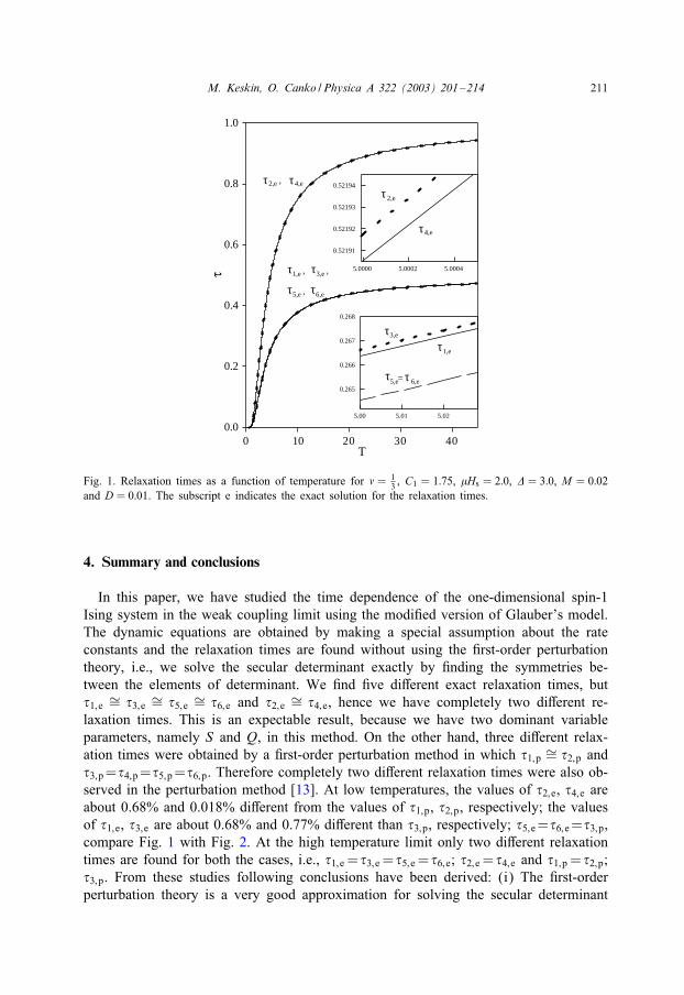
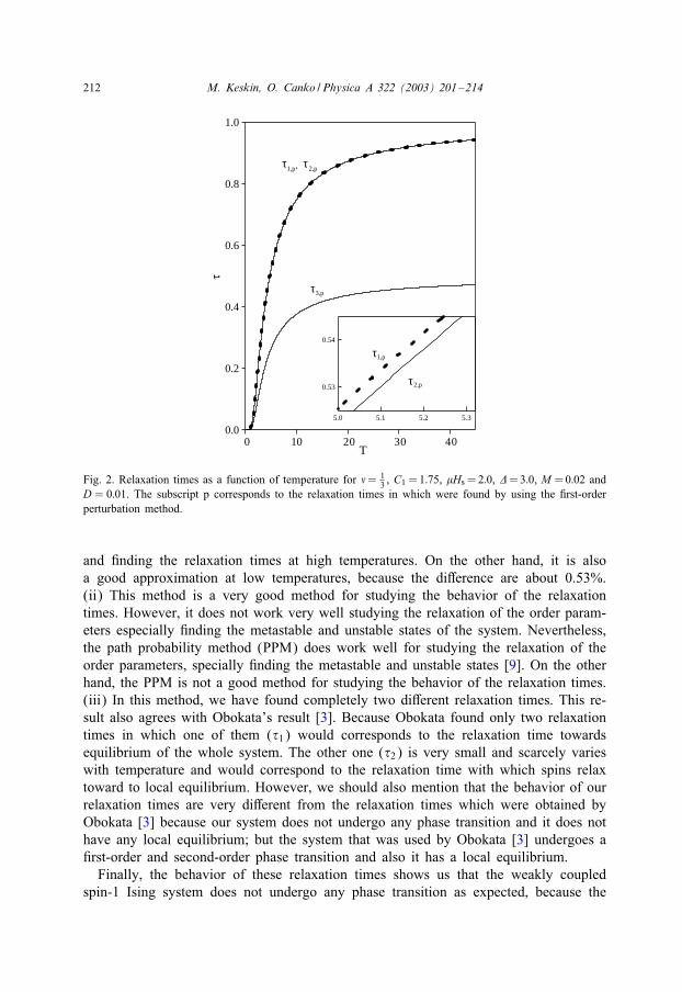
2Z�. The behav-iors of the relaxation times as a function of temperature are shown in Fig. 1 for theconstant values of �, C1, �Hs, �, D1 and D2. From these 1gures the following resultshave been found: (i) �1;e ∼= �3;e ∼= �5;e ∼= �6;e and �2;e ∼= �4;e, i.e., �1;e, �3;e, �5;e and�6;e are approximately equal to each other (see, the inset 1gure in Fig. 1) and also�2;e almost equal to �4;e, illustrated the inset 1gure in Fig. 1. The subscript e indicatesthe exact solution for the relaxation times. Therefore, we conclude that we have com-pletely two diCerent relaxation times. This is a expectable result, because we have twodominant variable parameters, namely S and Q, in this method. (ii) These relaxationtimes increase exponentially with the temperature at low temperatures and at high tem-peratures they relax, as seen in Fig. 1. (iii) �2;e and �4;e are more increasing than theother relaxations times at low temperatures. (iv) At very high temperatures limit onlytwo diCerent relaxation times are obtained, i.e., �1;e = �3;e = �5;e = �6;e and �2;e = �4;e.On the other hand, only three diCerent relaxation times were obtained by a 1rst-orderperturbation method in which �1;p and �2;p are approximately equal to each other (see,the inset 1gure in Fig. 2) and �3;p = �4;p = �5;p = �6;p are very diCerent than �1;p and�2;p, seen in Fig. 2. Thus, completely two diCerent relaxation times were also found bythe perturbation method [13]. We should also mention that at very high temperatures�1;p becomes equal to the �2;p, illustrated in Fig. 2. The subscript p corresponds to therelaxation times that were found by using the 1rst-order perturbation method [13].The discussion of the physical implications of these relaxation times will be given inthe last section.


T0 10 20 30 40

0.0

0.2

0.4

0.6

0.8

1.0

5.0000 5.0002 5.0004

0.52191

0.52192

0.52193

0.52194

5.00 5.01 5.02

0.265

0.266

0.267

0.268

2,e , 4,e

1,e , 3,e ,

5,e , 6,e

2,e

4,e

3,e

1,e

5,e= 6,e

τ ττ

τ

τ τ

ττ

τ τ

ττ

Fig. 1. Relaxation times as a function of temperature for � = 13 , C1 = 1:75, �Hs = 2:0, � = 3:0, M = 0:02

and D = 0:01. The subscript e indicates the exact solution for the relaxation times.

4. Summary and conclusions

In this paper, we have studied the time dependence of the one-dimensional spin-1Ising system in the weak coupling limit using the modi1ed version of Glauber’s model.The dynamic equations are obtained by making a special assumption about the rateconstants and the relaxation times are found without using the 1rst-order perturbationtheory, i.e., we solve the secular determinant exactly by 1nding the symmetries be-tween the elements of determinant. We 1nd 1ve diCerent exact relaxation times, but�1;e ∼= �3;e ∼= �5;e ∼= �6;e and �2;e ∼= �4;e, hence we have completely two diCerent re-laxation times. This is an expectable result, because we have two dominant variableparameters, namely S and Q, in this method. On the other hand, three diCerent relax-ation times were obtained by a 1rst-order perturbation method in which �1;p ∼= �2;p and�3;p=�4;p=�5;p=�6;p. Therefore completely two diCerent relaxation times were also ob-served in the perturbation method [13]. At low temperatures, the values of �2;e, �4;e areabout 0.68% and 0.018% diCerent from the values of �1;p, �2;p, respectively; the valuesof �1;e, �3;e are about 0.68% and 0.77% diCerent than �3;p, respectively; �5;e=�6;e=�3;p,compare Fig. 1 with Fig. 2. At the high temperature limit only two diCerent relaxationtimes are found for both the cases, i.e., �1;e = �3;e = �5;e = �6;e; �2;e = �4;e and �1;p = �2;p;�3;p. From these studies following conclusions have been derived: (i) The 1rst-orderperturbation theory is a very good approximation for solving the secular determinant


T0 10 20 30 40

0.0

0.2

0.4

0.6

0.8

1.0

5.0 5.1 5.2 5.3

0.53

0.54

1,p, 2,p

3,p

1,p

2,p

τ τ

τ

τ

τ

Fig. 2. Relaxation times as a function of temperature for �= 13 , C1 = 1:75, �Hs = 2:0, �=3:0, M =0:02 and

D = 0:01. The subscript p corresponds to the relaxation times in which were found by using the 1rst-orderperturbation method.

and 1nding the relaxation times at high temperatures. On the other hand, it is alsoa good approximation at low temperatures, because the diCerence are about 0.53%.(ii) This method is a very good method for studying the behavior of the relaxationtimes. However, it does not work very well studying the relaxation of the order param-eters especially 1nding the metastable and unstable states of the system. Nevertheless,the path probability method (PPM) does work well for studying the relaxation of theorder parameters, specially 1nding the metastable and unstable states [9]. On the otherhand, the PPM is not a good method for studying the behavior of the relaxation times.(iii) In this method, we have found completely two diCerent relaxation times. This re-sult also agrees with Obokata’s result [3]. Because Obokata found only two relaxationtimes in which one of them (�1) would corresponds to the relaxation time towardsequilibrium of the whole system. The other one (�2) is very small and scarcely varieswith temperature and would correspond to the relaxation time with which spins relaxtoward to local equilibrium. However, we should also mention that the behavior of ourrelaxation times are very diCerent from the relaxation times which were obtained byObokata [3] because our system does not undergo any phase transition and it does nothave any local equilibrium; but the system that was used by Obokata [3] undergoes a1rst-order and second-order phase transition and also it has a local equilibrium.Finally, the behavior of these relaxation times shows us that the weakly coupled

spin-1 Ising system does not undergo any phase transition as expected, because the


system, prepared an initial (non-equilibrium) state, always relaxes exponentially towardits equilibrium values. However if the system undergoes a second- or 1rst-order phasetransitions, at least one of the relaxation times should increase rapidly with increasingtemperature and tends to in1nity near the second-order phase transition temperature[4,11,23], but it makes a sharp cusp at the 1rst-order phase transition point [4,11].On the other hand, the other relaxation times scarcely vary with the temperature andthey increase slightly just below and above the second-order phase transition tempera-ture, but they display diCerent behavior at the 1rst-order phase transition temperature,just a jump discontinuity [4,11]. Nevertheless, the present calculation serves as an ex-ploratory model for the spin-1 Ising systems. Therefore, in order to study a cooperativephenomenon one should include the interaction parameters. This will be worked out ina subsequent paper.

Acknowledgements

This work was supported by NATO Grant No. CRG. 970008 1036/97. We thankProf. Dr. Paul H.E. Meijer for fruitful discussions and many helpful suggestions.

Appendix A. The self-consistent equations

We should give the following facts about the equilibrium of the system brie>y, inorder to understand the behavior of the time-dependence of the system, clearly. TheEquilibrium values for the probabilities, namely P∞(+), P∞(0), and P∞(−), are easilyfound using Eq. (2):

P∞(+) = Z−1e�+�; P∞(0) = Z−1; P∞(−) = Z−1e−�+� (A.1)

with the partition function de1ned by

Z = e�+� + 1 + e−�+� :

On the other hand, we can easily calculate the average magnetization or dipole moment〈S〉 and quadrupole moment 〈S2〉 ≡ 〈Q〉 at the equilibrium:

S∞ ≡ 〈S〉∞ =2 sinh �

e−� + 2 cosh �; (A.2)

Q∞ ≡ 〈Q〉∞ =2 cosh �

e−� + 2 cosh �≡ 〈S2〉∞ : (A.3)

References

[1] M. Keskin, C. Ekiz, O. YalUcVn, Physica A 267 (1999) 392;E. Albayrak, M. Keskin, J. Magn. Magn. Mater. 206 (1999) 83;E. Albayrak, M. Keskin, J. Magn. Magn. Mater. 203 (2000) 201;M. Keskin, C. Ekiz, J. Chem. Phys. 113 (2000) 5407, and references therein.


[2] C. Buzano, L.R. Evangelista, A. Pelizzola, Phys. Rev. B 53 (1996) 15063;A. Bakchich, M. El Bouziani, Phys. Rev. B 56 (1997) 1155;J. Ni, B.L. Gu, J. Phys. Condens. Matter 10 (1998) 5323, and references therein.

[3] T. Obokata, J. Phys. Soc. Jpn. 26 (1969) 895.[4] M. Tanaka, K. Takahashi, Prog. Theor. Phys. 58 (1977) 387;

M. Tanaka, K. Takahashi, J. Phys. Soc. Jpn. 43 (1977) 1832.[5] G.L. Batten, H.L. Lemberg, J. Chem. Phys. 70 (1979) 2934.[6] R. Zwanzig, Lect. Theor. Phys. 3 (1960) 106;

S. Nakajima, Prog. Theor. Phys. 20 (1958) 948.[7] Y. Saito, H. MJuller-Krumbhaar, J. Chem. Phys. 74 (1981) 721.[8] Y. Achiam, Phys. Rev. B 31 (1985) 260.[9] M. Keskin, P.H.E. Meijer, Physica A 122 (1983) 1;

M. Keskin, Physica A 135 (1986) 226;M. Keskin, M. ArV, P.H.E. Meijer, Physica A 157 (1989) 1000;M. Keskin, P.H.E. Meijer, J. Chem. Phys. 85 (1986) 7324;M. Keskin, R. Erdem, J. Stat. Phys. 89 (1997) 1035;M. Keskin, A. Solak, J. Chem. Phys. 112 (2000) 6396;C. Ekiz, M. Keskin, O. YalUcVn, Physica A 293 (2001) 215.

[10] R. Kikuchi, Suppl. Prog. Theor. Phys. 35 (1966) 1;K. Wada, M. Kaburagi, T. Uchida, R. Kikuchi, J. Stat. Phys. 53 (1988) 1081.

[11] R. Erdem, M. Keskin, Phys. Stat. Sol. B 225 (2001) 145;R. Erdem, M. Keskin, Phys. Rev. E 64 (2001) 026 102;M. Keskin, R. Erdem, Phys. Lett. A 297 (2002) 427.

[12] R. Erdem, M. Keskin, Phys. Lett. A 291 (2001) 159.[13] M. Keskin, P.H.E. Meijer, Phys. Rev. E 55 (1997) 5343.[14] R. Glauber, Bull. Am. Phys. Soc. 5 (1960) 296;

R. Glauber, J. Math. Phys. 4 (1963) 294.[15] P.H.E. Meijer, T. Tanaka, J. Barry, J. Math. Phys. 3 (1962) 793.[16] Z.R. Yang, Phys. Rev. B 46 (1992) 11 578;

A. Prados, J.J. Brey, preprint, arXiv:cond-mat/0106236, 2001;B.C.S. Grandi, W. Figueiredo, Phys. Rev. B 50 (1994) 12 595;J.J. Brey, A. Prados, preprint, arXiv:cond-mat/0105232, 2001;J.H. Luscombe, M. Luban, J.P. Reynolds, Phys. Rev. E 53 (1996) 5852;A. Caneschi, D. Gatteschi, N. Lalioti, C. Sangregorio, R. Sessoli, G. Venturi, A. Vindigni, A. Rettori,M.G. Pini, M.A. Novak, preprint, arXiv:cond-mat/0106224, 2001;J.J. Brey, A. Prados, Phys. Rev. E 53 (1996) 458;A. Prados, J.J. Brey, J. Phys. A: Math. Gen. 34 (2001) L453;A. Crisanti, H. Sompolinsky, Phys. Rev. A 37 (1988) 4865;U.L. Fulco, L.S. Lucena, G.M. Viswanathan, Physica A 264 (1999) 171.

[17] E.W. Montroll, Proc. Natl. Acad. Sci. USA 78 (1) (1981) 36;Y. Ma, J. Liu, Phys. Lett. A 238 (1998) 159;G. Forgacs, D. Mukamel, R.A. Pelcovits, Phys. Rev. B 30 (1984) 205.

[18] J. Wang, Phys. Rev. B 47 (1993) 869;Y. Achiam, Phys. Rev. B 19 (1979) 376;T. Vojta, J. Phys. A: Math. Gen. 30 (1997) L7;T. Vojta, J. Phys. A: Math. Gen. 30 (1997) L643;T. Tome, M.J. Oliveira, Phys. Rev. A 41 (1990) 4251;A. Bovier, F. Manzo, ArXiv:cond-mat/0107376, 2001.

[19] G.M. Buendia, E. Machado, Phys. Rev. E 58 (1998) 1260.[20] B. Derrida, R. Zeitak, Phys. Rev. E 54 (1996) 2513.[21] B.U. Felderhof, Rep. Math. Phys. 1 (1970) 219.[22] F.C. Alcaraz, M. Droz, M. Henkel, V. Rittenberg, Ann. of Phys. 230 (1994) 250.[23] H.E. Stanley, Introduction to Phase Transitions and Critical Phenomena, Clarendon Press, Oxford, 1971.

time dependence of the weakly coupled spin-1 ising system using the glauber model

Documents