time consistency in option pricing models - kth · pdf fileattempts have been made to...
TRANSCRIPT

Time Consistency in Option Pricing Models
Johan Nykvist
October 30, 2009

Abstract
Since the introduction of the famous Black-Scholes model (1973), severalattempts have been made to construct option pricing models that allow fornon-gaussian return distributions as well as varying volatilities. In this the-sis, we examine the robustness of two of these models in terms of the timeconsistency, or possibly inconsistency, of the model parameters. We restrictour attention to the stochastic volatility model provided by Heston (1993)and the local volatility model introduced by Dupire (1994). We estimatethe models daily in order to �nd parameters that match the current marketprices as closely as possible, hence the calibration process constitutes a ma-jor part of the thesis. Our results show that both models are succesful inexplaining important characteristics of the implied volatility surface, whenthe market conditions are fairly stable. On the other hand, when the marketis heavily �uctuating, both models reveal a high degree of time inconsistency,as they are unable to capture the current market conditions without largeparameter variations. In addition, the use of principal component analysisshows that variations of the local volatility surface, to a large extent can beexplained by three distinct movements.

Acknowledgements
I would like to thank my tutor Filip Lindskog for helpful advice during thewriting of this thesis. I am also grateful to Jonas Kiessling for valuablesuggestions.
Stockholm, October 2009
Johan Nykvist
iv

Contents
1 Introduction 1
2 Model Introduction and Data 3
2.1 The Heston Model: Stochastic volatility . . . . . . . . . . . . 32.2 Heston Continued . . . . . . . . . . . . . . . . . . . . . . . . . 62.3 The Dupire Model - Local Volatility . . . . . . . . . . . . . . 92.4 Data description . . . . . . . . . . . . . . . . . . . . . . . . . 11
3 The Calibration Problem 13
3.1 Calibrating Heston in Theory . . . . . . . . . . . . . . . . . . 133.2 Calibrating Heston in Practice . . . . . . . . . . . . . . . . . 153.3 Calibrating Dupire . . . . . . . . . . . . . . . . . . . . . . . . 18
4 Calibration Results 23
4.1 The Heston Model . . . . . . . . . . . . . . . . . . . . . . . . 234.2 The Dupire Model . . . . . . . . . . . . . . . . . . . . . . . . 27
5 Conclusions 33
A Results 37
A.1 Principal Component Analyis . . . . . . . . . . . . . . . . . . 37
B Matlab code 39
B.1 Calibrating the Heston model using Di�erential Evolution . . 39B.2 Calibrating the Heston model using lsqnonlin . . . . . . . . . 42B.3 Calibrating the Dupire model using lsqnonlin . . . . . . . . . 44
v

vi

Chapter 1
Introduction
Since the introduction of the famous Black-Scholes model (1973), severalattempts have been made to construct alternative option pricing models thatallow for non-gaussian return distributions as well as non-constant volatility.Models that allow negative correlation between the underlying stock priceand its volatility are examples of such models that are commonly found inthe literature.
The development of more sophisticated models however comes at thecost of increased complexity. While the Black-Scholes model only have oneunknown parameter, stochastic volatility models typically have between �veand �fteen parameters that have to be estimated. Consequently, the calibra-tion of such models is in general far more troublesome than calibrating theoriginal model proposed by Black and Scholes.
The performance of stochastic volatility models, in terms of pricing andhedging performance, has been investigated in a large number of papers (seefor example Bakshi, Cao and Chen (1997), Christo�ersen, Heston and Jacobs(2009) or Shoutens, Simons and Tistaert (2003)). What remains unexaminedhowever is the time consistency, or possibly inconsistency, of these models interms of parameter variations over time. From a theoretical point of view,a robust model would allow �uctuations in the underlying asset with theparameters remaining fairly constant. Large variations in daily parameterestimates would reduce the usefulness of these models as daily recalibrationsare both time consuming and may lead to large daily variations in moreexotic contracts (Schoutens, Simons and Tistaert (2003)).
In this thesis we aim to investigate the time consistency of alternative op-tion pricing models. We restrict our attention to the single factor stochasticvolatility model proposed by Heston (1993) and the local volatility functionintroduced by Dupire (1994). The models are applied to a number of putand call options written on the Euro Stoxx 50 index between June 23rd andDecember 31st 2008.
In Chapter 2 we introduce the two models and provide the theoretical
1

framework needed to proceed with the calibration problem. Since calibrationof stochastic volatility models is quite complex, a thorough discussion ofdi�erent approaches is provided in Chapter 3. In Chapter 4 we present themain results from the empirical study and discuss some of the implicationson option pricing theory. In the last chapter we summarize the materialcovered in the thesis and suggest topics for further studies.
2

Chapter 2
Model Introduction and Data
2.1 The Heston Model: Stochastic volatility
Assume that the spot price follows the di�usion
dS(t) = µS(t)dt+√v(t)S(t)dW1(t), S(0) = S0,
where W1(t) is a Wiener process. If the volatility follows an Ornstein-Uhlenbeck process,
d√v(t) = −β
√v(t)dt+ δdW2(t),
where W2(t) has correlation ρ with W1(t), then Itô's lemma shows that thevariance v(t) follows the process,
dv(t) = [δ2 − 2βv(t)]dt+ 2δ√v(t)dW2(t), V (0) = V0.
This process may be rewritten as
dv(t) = κ[θ − v(t)]dt+ σ√v(t)dW2(t),
which is known as a square root mean reverting process, �rst used by Cox,Ingersoll and Ross (1985), with long-run mean θ, and rate of reversion κ. σis referred to as the volatility of the volatility.
For κ, θ > 0, this corresponds to a process where the randomly movingvolatility is elastically pulled toward a long-term value, θ. The parameter κdetermines the speed of adjustment. In addition, if 2κθ ≥ 0, the volatilityprocess is always larger than zero (see Cox, Ingersoll and Ross (1985) orFeller (1951)).
Earlier research shows that there are both economical as well as em-pirical reasons for a model of this structure. Firstly, implied Black-Scholesvolatilities vary both with time to maturity and with strike price, so modelingvolatility as a random variable is a rather natural approach. Secondly, empir-ical studies indicate that an asset's log-return distribution is non-Gaussian,
3

characterized by heavy tails. This behavior is captured in the Heston modelby the parameter ρ. Intuitively, if ρ > 0, the volatility will increase as theasset return increases. This will spread the right tail and squeeze the left tailof the distribution creating a distribution with a fat right tail. The oppositeis of course true. In fact, there is evidence that the correlation between assetreturns and implied volatility is negative, also known as the 'leverage e�ect'.ρ, therefore, a�ects the skewness of the distribution. Finally, a phenomenaknown as 'volatility clustering' has been readily observed in the market. Ba-sically, it means that large price variations are more likely to be followedby large price variations and vice versa. In the Heston model, the meanreversion parameter κ can also be interpreted as representing the degree of'volatility clustering'.
Thus, there are several economical as well as theoretical arguments forthis choice of model. The main advantage of the Heston model, however, isthe closed-form solution for European call options. In the next section, wederive the general valuation equation and apply it to the Heston model inorder to obtain a pricing formula for European calls.
2.1.1 Derivation of the Valuation Equation
In this section, we follow the work of Gatheral (2006) closely. We begin byassuming that the spot price and the volatility follow the di�usions
dS(t) = µS(t)dt+√v(t)S(t)dW1(t), (2.1)
dv(t) = α(S(t), v(t), t)dt+ ηβ(S(t), v(t), t)√v(t)dW2(t), (2.2)
where
〈dW1(t), dW2(t)〉 = ρdt.
In contrast with the Black-Scholes model there are two sources of random-ness, the stock price and the volatility. Thus, in order to form a risklessportfolio we set up a portfolio Π containing the option being priced, whosevalue we denote by V (S, v, t), a quantity −∆ of the stock and a quantity−∆1 of another asset whose value V1 depends on volatility. We have
Π = V −∆S −∆1V1.
For the next step we need the following proposition (see Björk (2004), p.56):
Proposition 2.1. Take a vector Wiener process W = (W1, ...,Wn) with
correlation matrix ρ as given, and assume that the vector process X =(X1, ..., Xk) has a stochastic di�erential. Then the following hold:
4

For any C1,2 function f , the stochastic di�erential of the process f(t,X(t))is given by
df(t,X(t)) =∂f
∂tdt+
n∑i=1
∂f
∂xidXi +
12
n∑i,j=1
∂2f
∂xi∂xjdXidXj ,
with the formal multiplication table(dt)2 = 0,dt · dWi = 0, i = 1, ..., n,dWi · dWj = ρijdt.
Applying this proposition shows that the change in Π in a time dt isgiven by
dΠ =
{∂V
∂tdt+
12vS2∂
2V
∂S2+ ρηvβS
∂2V
∂v∂S+
12η2vβ2∂
2V
∂v2
}dt
−∆1
{∂V1
∂t+
12vS2 ∂V1
∂S2+ ρηvβS
∂2V1
∂v∂S+
12η2β2v
∂2V1
∂v2
}dt
+{∂V
∂S−∆1
∂V1
∂S−∆
}dS
+{∂V
∂v−∆1
∂V1
∂v
}dv
To make the portfolio instantaneously risk-free, we must choose
∂V
∂S−∆1
∂V1
∂S−∆ = 0
∂V
∂v−∆1
∂V1
∂v= 0
to eliminate dS terms and dv terms respectively. This leaves us with
dΠ =
{∂V
∂tdt+
12vS2∂
2V
∂S2+ ρηvβS
∂2V
∂v∂S+
12η2vβ2∂
2V
∂v2
}dt
−∆1
{∂V1
∂t+
12vS2 ∂V1
∂S2+ ρηvβS
∂2V1
∂v∂S+
12η2β2v
∂2V1
∂v2
}dt
= rΠdt= r(V −∆S −∆1V1)dt,
where we have used the fact that the return on a risk-free portfolio mustequal the risk-free rate r. Collecting all V terms on the left-hand side and
5

all V1 terms on the right-hand side, we get
∂V∂t + 1
2vS2 ∂2V∂S2 + ρηvβS ∂V
∂v∂S + 12η
2vβ2 ∂2V∂v2
+ rS ∂V∂S − rV∂V∂v
=∂V1∂t + 1
2vS2 ∂2V1∂S2 + ρηvβS ∂V1
∂v∂S + 12η
2vβ2 ∂2V1∂v2
+ rS ∂V1∂S − rV1
∂V1∂v
.
The left-hand side is a function of V only and the right-hand side is a functionof V1 only. Thus, we conclude that both sides must be equal to some functionf of the independent variables S, v and t. We deduce that
∂V
∂t+
12vS2∂
2V
∂S2+ ρηvβS
∂V
∂v∂S+
12η2vβ2∂
2V
∂v2+ rS
∂V
∂S− rV
= −(α− φβ
√v) ∂V∂v
(2.3)
where, without loss of generality, we have written the arbitrary function f ofS, v and t as (α−φβ
√v)∂V∂v . φ(S, v, t) is called the market price of volatility
risk. Now, de�ning the risk-neutral drift as
α′ = α− β√vdZ2
we see that, as far as pricing of options is concerned, we could have startedwith the risk-neutral SDE for v,
dv = α′dt+ β√vdZ2 (2.4)
and got identical results with no explicit price of risk term because we arein the risk-neutral world. In what follows, we assume that the SDEs for Sand v are in risk-neutral terms because we are invariably interested in �ttingmodels to option prices.
2.2 Heston Continued
The Heston model corresponds to choosing α(S(t), v(t), t) = κ(θ − v(t))and β(S(t), v(t), t) = 1 in equations (2.1) and (2.2). These equations thenbecome
dS(t) = µS(t)dt+√v(t)S(t)dW1(t)
and
dv(t) = κ(θ − v(t))dt+ σ√v(t)dW2(t)
with
〈dW1(t), dW2(t)〉 = ρdt
6

where κ is the speed of reversion of v(t) to its long-term mean θ. We nowsubstitute the above values for α(S(t), v(t), t) and β(S(t), v(t), t) into thegeneral valuation equation. We obtain
∂V
∂t+
12vS2∂
2V
∂S2+ ρσvS
∂2V
∂v∂S+
12σ2v
∂2V
∂v2+ rS
∂V
∂S− rV
= −κ(θ − v)∂V
∂v(2.5)
In Heston's original paper, the price of risk is assumed to be linear in thevariance v. In contrast, we assume that the Heston process, with parameters�tted to option prices, generates the risk-neutral measure so the market priceof volatility risk φ in the general valuation equation (2.3) is set to zero. Sincewe are only interested in pricing, and we assume that the pricing measure isrecoverable from European option prices, we are indi�erent to the statisticalmeasure.
2.2.1 The Heston Solution for European Options
A European call option with strike price K and maturing at time T satis-�es the partial di�erential equation (2.5) subject to the following boundaryconditions:
V (S, v, T ) = max(S −K, 0),V (0, v, t) = 0,
∂V
∂S(∞, v, t) = 1, (2.6)
rS∂V
∂S(S, 0, t) + κθ
∂V
∂v(S, 0, t)− rV (S, 0, t) +
∂V
∂t(S, 0, t) = 0,
V (S,∞, t) = S
In analogy with the Black-Scholes formula, for the European call option,whose value we denote C(S, v, t) we guess a solution of the form
C(S, v, t) = SP1 −KP (t, T )P2, (2.7)
where the �rst term is the present value of the spot price upon optimalexercise, and the second term is the present value of the strike-price payment.P (t, T ) is the price at time t of a zero-coupon bond maturing at time T withface value 1. Both of these terms must satisfy the original PDE (2.5). If wede�ne x = lnS and substitute the proposed solution (2.7) into the originalPDE (2.5) we see that P1 and P2 must satisfy the PDEs
12v∂2Pj∂x2
+ ρσv∂2Pj∂x∂v
+12σ2v
∂2Pj∂v2
+ (r + ujv)∂Pj∂x
+ (aj − bjv)∂Pj∂v
+∂Pj∂t
= 0, (2.8)
7

for j = 1, 2, where
u1 = 1/2, u2 = −1/2, a = κθ, b1 = κ− ρσ, b2 = κ.
Given the boundary conditions for the option price in equation (2.6), thesePDEs (2.8) are subject to the terminal condition
Pj(x, v, T ; lnK) = 1{x≥lnK}.
Thus, they may be interpreted as "adjusted" or "risk-neutralized" proba-bilities (see Cox and Ross (1976)). To see why, assume that x(t) and v(t)follows the stochastic process
dx(t) = (r + ujv)dt+√v(t)dz1(t),
dv(t) = (aj − bjv)dt+ σ√v(t)dz2(t),
where the parameters uj , aj , and bj are de�ned as before. Further, considerany twice-di�erentiable function f(x, v, t) that is a conditional expectationof some function of x and v at a later date, T , g(x(T ), v(T )):
f(x, v, t) = E[g(x(T ), v(T ))|x(t) = x, v(t) = v]. (2.9)
Using Itô's lemma we get
df =
(12v∂2f
∂x2+ ρσv
∂2f
∂x∂v+
12σ2v
∂2f
∂v2+ (r + ujv)
∂f
∂x+ (a− bjv)
∂f
∂v+∂f
∂t
)dt
+ (r + ujv)∂f
∂xdz1 + (a− bjv)
∂f
∂vdz2. (2.10)
By iterated expectations, we know that f must be a martingale, in par-ticular, E[df ] = 0. Applying this to equation (2.10) yields the well-knownFokker-Planck forward equation:
12v∂2f
∂x2+ ρσv
∂2f
∂x∂v+
12σ2v
∂2f
∂v2
(r + ujv)∂f
∂x+ (a− bjv)
∂f
∂v+∂f
∂t= 0
Equation (2.9) imposes the terminal condition
f(x, v, T ) = g(x, v).
Now, if g(x, v) = 1{x≥lnK}, then the solution is the conditional probability
at time t that x(T ) is greater than lnK. In addition, if g(x, v) = eiφx, thenthe solution is the characteristic function E[eiφx(T )|x(t) = x, v(t) = v]. Theprobabilities are not immediately available in closed form. However, Hes-ton shows that their characteristic functions, f1(x, v, T ;φ) and f2(x, v, T, φ)respectively, satisfy the same PDEs (2.8), subject to the terminal condition
fj(x, v, T ;φ) = eiφx.
8

The characteristic function solution is
fj(x, v, T ;φ) = eC(T−t;φ)+D(T−t;φ)v+iφx, (2.11)
where
C(τ ;φ) = rφiτ +a
σ2
(bj − ρσφi+ d)τ − 2ln
[1− gedτ)
1− g
] ,
D(τ ;φ) =bj − ρσφi+ d
σ2
[1− edτ
1− gedτ
],
and
g =bj − ρσφi+ d
bj − ρσφi− d,
d =√
(ρσφi− bj)2 − σ2(2ujφi− φ2).
One can invert the characteristic functions to get the desired probabilities:
Pj(x, v, T ; lnK) =12
+1π
∫ ∞0
Re
[e−iφlnKfj(x, v, t;φ)
iφdφ
]. (2.12)
The integrand in equation (2.12) is a smooth function that decays rapidly.Equations (2.7), (2.11), and (2.12) give the solution for European call op-tions.
2.3 The Dupire Model - Local Volatility
Given the computational complexity of stochastic volatility models and thedi�culty of parameter �tting to plain vanilla options, practitioners soughta simpler way of pricing options consistently with the volatility skew. Thebreakthrough came when Dupire (1994) and Derman and Kani (1994) notedthat under risk neutrality, there was a unique di�usion process consistentwith the risk-neutral density derived from the market prices of Europeanoptions. The corresponding unique di�usion coe�cient σL(S, t) is known asthe local volatility function. In the next section we review the original workof Dupire and derive an explicit expression for the local volatility function.
2.3.1 Derivation of the Dupire Equation
Suppose the stock price di�uses with risk-neutral drift µ(t) = r(t) − D(t)and local volatility σ(S, t) according to the equation
dS(t)S(t)
= µ(t)dt+ σ(S(t), t)dW (t),
9
where r(t) is the risk-free interest rate, D(t) is the dividend yield and W (t)is a Wiener process. The risk-neutral expected value C∗(S0,K, T ) of a Eu-ropean option payo� with strike K and expiration T is given by
C∗(S0,K, T ) =∫ ∞
0ϕ(ST , T ;S0)(ST −K)+dST , (2.13)
where ϕ(ST , T ;S0) is the probability density of the �nal spot at time T .For a process with drift D1(x, t) and di�usion D2(x, t) the probability den-sity function evolves over time according to the Fokker-Planck equation (orForward Kolmogorov equation) (see Gatheral (2006)):
∂
∂t= − ∂
∂x[D1(x, t)ϕ(x, t)] +
∂2
∂x2[D2(x, t)ϕ(x, t)].
Thus, in the Dupire model the probability density evolves according to theequation
∂ϕ
∂T=
12∂2
∂S2T
(σ2S2
Tϕ)− ∂
∂ST(µSTϕ)
Di�erentiating (2.13) with respect to K gives
∂C∗
∂K= −
∫ ∞K
ϕ(ST , T ;S0)dST
∂2C∗
∂K2= ϕ(K,T ;S0)
Now, di�erentiating (2.13) with respect to time gives
∂C∗
∂T=∫ ∞K
{∂
∂Tϕ(ST , T ;S0)
}(ST −K)dST
=∫ ∞K
{12∂2
∂S2T
(σ2S2
Tϕ)− ∂
∂ST(µSTϕ)
}(ST −K)dST
Integrating by parts twice gives:
∂C∗
∂T=σ2K2
2ϕ+
∫ ∞K
µSTϕdST
=σ2K2
2∂2C∗
∂K2+ µ(T )
(−K∂C∗
∂K
),
which is the Dupire equation when the underlying stock has risk-neutral driftµ. Formally, we can solve for the volatility to get
σ2(S, t) =∂C∗
∂T + µ(T )K ∂C∗
∂K12K
2 ∂2C∗
∂K2
∣∣∣∣∣K=S,T=t
(2.14)
10

The right-hand side of equation (2.14) can be computed from known Euro-pean option prices. So, given a complete set or European option prices forall strikes and expirations, local volatilities are given uniquely by equation(2.14). Alternatively, assuming that the call price is a function of the impliedBlack and Scholes volatility, i.e. C = CBS(S0, t, T,K, σI), we may calculatethe derivatives using the chain-rule and obtain an expression for the localvolatility in terms of implied volatilies (see Elder (2002)):
σ2(S, T ) =σ2I + 2σI(T − t)
(∂σI
∂T + (r −D)K ∂σI
∂K
)(
1 +Kd1∂σI
∂K
√T − t
)2
+ σ2IK
2(T − t)(∂2σI
∂K2 − d1
(∂σI
∂K
)2√T − t
)∣∣∣∣∣K=S,T=t
where
d1 =ln(S0/K) + (r + σ2/2)(T − t0)
σ√T − t0
.
Thus, we have established the theoretical framework needed to proceed withthe calibration problem. Before that, however, we present the market dataused in the calibration process and discuss some of the di�culties with realmarket data.
2.4 Data description
The data used for the analysis are European style put and call options writtenon the Euro Stoxx 50 index during the period June 23rd to December 30th
2008. The chosen time period is interesting for a number of reasons. Duringthe �rst three months, the market is stable with only small �uctuations inthe underlying asset. However, the last three months constitute a period ofextreme movements on the stock market due to the �nancial crisis last year.Thus, the robustness of the models in terms of parameter variations will betested in a period when market conditions vary signi�cantly.
The initial data set consists of four put and twenty call options on theindex during the time period speci�ed above. For all options we extractinformation about maturity, strike price and current index level. The con-tracts chosen are the most frequently traded options on the index duringthe time period, making them reliable for the calibration procedure. All inall the set of options consists of contracts with �ve di�erent strikes (rangingfrom 2500 to 3500) and four di�erent maturities where, on the �rst date,the option maturities range from 1 year to 2.5 years. Then, as we monitorthese options over time, the maturities decrease continuously, hopefully en-abling us to capture the dependence of changes in market expectations onthe parameter estimates of the two models.
The yield curve is constructed by a cubic spline interpolation betweenEuribor quotes of maturities ranging from 1 month to 2 years. All interestrates are assumed to be continuously compounded. The dividend yields are
11

Figure 2.1: The left plot shows the Euro Stoxx 50 index during the sampleperiod and the right plot shows the corresponding log returns. Note thelarge �uctuations in the spot prices during the last quarter of 2008.
then obtained using the put-call parity (see Section 3.2), where we make useof the fact that on each day we have both put and call prices for the samestrike and maturity, which enables us to solve for the implied dividend yield.
12

Chapter 3
The Calibration Problem
3.1 Calibrating Heston in Theory
We analyze the model in terms of the risk-neutral volatility process describedin equation (2.4), because the risk-neutral process exclusively determinesprices. Calibrating the Heston model is equivalent to �nding the parametersκ, θ, σ, ρ and the spot variances V0 which produce the correct market prices.Option pricing models are usually calibrated to market data by minimizationof an error functional, i.e. by solving an optimization problem of the form
Θ̂ = arg minΘL[{C}n, {C(Θ,Λ)}n],
where Θ is the parameter vector and Λ is the vector of spot variances.{C(Θ,Λ)
}nis a set of n option prices obtained from the model, {C}n is
the corresponding set of observed option prices in the market and L is someloss function. From an economic viewpoint, there are several possibilitiesto measure the error between the market and the model. These di�erentspeci�cations of the error lead to di�erent sets of calibrated model parame-ters and the resulting pricing performance may vary signi�cantly (Shoutens,Simons and Tistaert (2003)).
3.1.1 The Choice of Loss Function
The most frequently used loss functions in the literature are the dollar meansquared error ($ MSE), the percentage mean squared error (% MSE), and
13

the implied volatility mean squared error (IV MSE):
$MSE(Θ,Λ) =n∑i=1
wi(Ci − Ci(Θ,Λ))2;
%MSE(Θ,Λ) =n∑i=1
wi
(Ci − Ci(Θ,Λ)
Ci
)2
;
IV MSE(Θ,Λ) =n∑i=1
wi(σi − σi(Θ,Λ))2,
where σi is the Black-Scholes implied volatility of option i, and σi(Θ,Λ)denotes the corresponding Black-Scholes implied volatility obtained usingthe model price as input. wi is an appropriately chosen weight, which willbe discussed in more detail below.
The choice of loss function is important and has many implications. The$ MSE function minimizes the squared dollar error between model prices andmarket prices and will thus favor parameters that correctly price expensiveoptions. In contrast, the % MSE function adjusts for price level, and willinstead focus on options with prices close to zero. The IV MSE functionon the other hand minimizes implied volatility errors, and will thereforefavor options with high implied volatilities. Detlefsen and Härdle (2006)has studied four di�erent error functionals and suggest that once a suitablemodel has been chosen the IV MSE function is best suited for calibratingthe model parameters. On the other hand, if there is uncertainty about thecorrectness of the model, the authors suggests using the $ MSE function.
Since we are interested in the parameter variations over time, all threeloss function will be used during the calibration process. Hopefully, this willlead to a more profound understanding of the dynamics contained in theHeston model.
3.1.2 The Choice of Weights
Earlier research (e.g. Mikhailov and Nögel (2003)) has shown that the choiceof weighting wi has a large in�uence on the error functional, and thereforeon the parameter estimates. Two common methods are to either use thebid-ask spread of the options or to choose weights according to the numberof options within di�erent maturity categories. Using wi = 1
|bidi−aski| is arather intuitive approach. If the bid-ask spread is large, there is a greatuncertainty about the true price of the option and we assign it less weight.Since bid and ask prices may be hard to come by, this method is sometimesdi�cult to use. An alternative approach is to choose weights so that oneach day all maturities have the same in�uence on the objective function.Moreover, the same weight is assigned to all points of the same maturity.
14

This leads to the weights
wi =1
nmatnistr
where nmat denotes the number of maturities, and nistr denotes the numberof strikes with the same maturity as observation i.
3.1.3 Regularization
In addition to the objective function that is minimized we add a regular-ization term. Regularization can be necessary for two reasons: Most com-monly proposed error functionals may have several global minima (Cont andHamida (2005)) and thus the regularization term is needed to get a uniqueminimum. Also, it is important to �nd parameters on subsequent days thatlead to similar prices of exotic options. This is essential for the practicalapplicability of the model. Moreover, adding a regularization term may pro-vide additional stability to the calibration. In accordance with Mikhailovand Nögel we add a regularization term and minimize the following function
L({C}n, {C(Θ,Λ)}n) + α|Θ−Θ0|,
where Θ0 is the initial parameter vector. The choice of α is important andmay have severe implications on the pricing performance of the model. Ifα is chosen large, the di�erence between market and model prices has littleimpact on the total value of the error functional, and over time the pricingperformance may decrease. On the other hand, if α is chosen small, theparameters may exhibit rough oscillations leading to large �uctuations inexotic option prices (see Schoutens, Simons and Tistaert (2003)).
3.2 Calibrating Heston in Practice
To calculate model prices in practice we note that the call price is not onlya function of the parameters κ, θ, σ, ρ, and V0, but also of the strike price K,the time to maturity T , the risk-free interest rate r and the dividend yield δ.The strike price and the time to maturity is uniquely speci�ed by the contractin question, but the risk-free interest rate and the dividend yield have to beapproximated in some way. Firstly, we approximate the yield curve usingthe Euribor. These are given for six di�erent maturities (1 month, 2 months,3 months, 6 months, 1 year, and 2 years). Then, for any maturity betweenthese values we can �nd the corresponding interest rate by some suitableinterpolation technique. To approximate the dividend yield we assume thatthe dividends of the Euro Stoxx 50 index are paid continuously. Then, usingthe next proposition we may solve for the corresponding dividend yield.
Proposition 3.1. (Put-Call Parity when the Underlying pays a ContinuousDividend) Let Cδ(Pδ) denote the price of a European call (put) and let r
15

denote the risk-free interest rate, δ denote the dividend yield, S be the price
of the underlying, and K be the strike price. Then, the following relation
holds:
Pδ = Cδ − Se−δ(T−t) +Ke−r(T−t)
Proof. Consider a portfolio Π1 that consists of one long position in a calloption and Ke−r(T−t) long positions in zero coupon bonds, i.e.
Π1 = Cδ +Ke−r(T−t).
The value of this portfolio at time T is given by{S −K +K = S, if S ≥ K
0 +K = K, if S ≤ K
Next, consider a portfolio Π2 that consists of one long position in a putoption and Se−δ(T−t) long positions in the underlying stock, i.e.
Π2 = P + Se−δ(T−t)
The value of this portfolio at time T is given by{0 + S = S, if S ≥ K
K − S + S = K, if S ≤ K
Since we assume the absence of arbitrage, the present value of the two port-folios must be equal, and this completes the proof.
Now, for each date we have prices for four call options and four putoptions on the same underlying asset, with the same strike price and thesame time to maturity. Thus, using the proposition above we may solve forthe dividend yield to get
δ =−1T − t
ln
(Cδ − Pδ +Ke−r(T−t)
S
)
Then, we know the risk-neutral drift µ(t) = r(t) − δ(t) for four di�erentmaturities. Using a smooth cubic spline we interpolate from these values toobtain the drift term for all maturities. Thus, we have obtained all inputparameters needed to calculate the model prices. The next step is to solvethe optimization problem.
16
3.2.1 The Optimization Problem
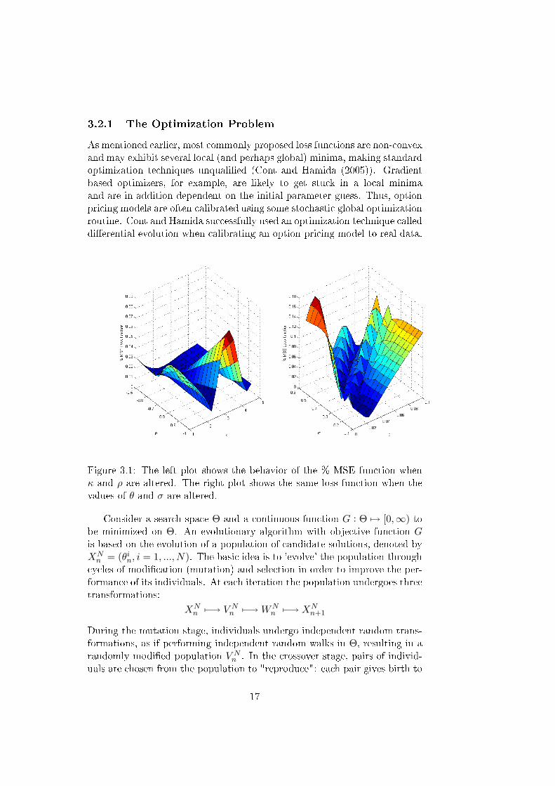
As mentioned earlier, most commonly proposed loss functions are non-convexand may exhibit several local (and perhaps global) minima, making standardoptimization techniques unquali�ed (Cont and Hamida (2005)). Gradientbased optimizers, for example, are likely to get stuck in a local minimaand are in addition dependent on the initial parameter guess. Thus, optionpricing models are often calibrated using some stochastic global optimizationroutine. Cont and Hamida successfully used an optimization technique calleddi�erential evolution when calibrating an option pricing model to real data.
Figure 3.1: The left plot shows the behavior of the % MSE function whenκ and ρ are altered. The right plot shows the same loss function when thevalues of θ and σ are altered.
Consider a search space Θ and a continuous function G : Θ 7→ [0,∞) tobe minimized on Θ. An evolutionary algorithm with objective function Gis based on the evolution of a population of candidate solutions, denoted byXNn = (θin, i = 1, ..., N). The basic idea is to 'evolve' the population through
cycles of modi�cation (mutation) and selection in order to improve the per-formance of its individuals. At each iteration the population undergoes threetransformations:
XNn 7−→ V N
n 7−→WNn 7−→ XN
n+1
During the mutation stage, individuals undergo independent random trans-formations, as if performing independent random walks in Θ, resulting in arandomly modi�ed population V N
n . In the crossover stage, pairs of individ-uals are chosen from the population to "reproduce": each pair gives birth to
17

a new individual, which is then added to the population. This new popula-tion, WN
n is now evaluated using the objective function G(·). Elements ofthe population are now selected for survival according to their �tness: thosewith a lower value of G have a higher probability of being selected. TheN individuals thus selected then form the new population XN
n+1. The roleof mutation is to explore the parameter space and the optimization is donethrough selection.
There is no proof of convergence for algorithms based on di�erential evo-lution. However, several comparisons have shown that DE is more accurateand more e�cient than several other optimisation techniques including simu-lated annealing and evolutionary programming. On the downside, stochasticoptimization techniques are generally much more time consuming than forexample gradient based optimizers. Therefore, we will make use of both al-ternatives. We use the DE algorithm for the �rst date to get reliable results.After that we will solve the optimization problem using Matlab's algorithmlsqnonlin, which is a gradient based optimizer. On one hand, we risk gettingstuck in a local minima. On the other hand, unless the market has changeddramatically we do not expect the parameters to change very much. Inperiods when the stock price �uctuates heavily we will again use the DEalgorithm to obtain reliable parameter estimates.
The Matlab code needed to calibrate the Heston model is included in theAppendix. Despite the fact that the formulae look quite complicated, the cal-ibration of the model is rather straightforward. In this thesis, the integrandin equation (2.12) was calculated using the Matlab function quadl. Carr andMadan (1999) present another approach for numerically determining optionvalues, provided that the characteristic function of the risk-neutral densityis known. The scheme uses the Fast Fourier Transform (FFT), leading tomuch faster calculations compared to other numerical integration schemes.Thus, when a large number of options is used in the calibration, the FFTmay lead to large reductions in computation time. Because we only used25 options in the calibration, and also because the Matlab function is moreeasily implemented, we chose not to use FFT in the calculations.
3.3 Calibrating Dupire
At �rst glance, the calibration of the local volatility function seems straight-forward. Given a complete set of European option prices for all strikes andall expirations, local volatilities are given uniquely by
σ2(S, T ) =∂C∂T + µ(T )K ∂C
∂K12K
2 ∂2C∂K2
∣∣∣∣∣K=S,T=t
(3.1)
In practice, however, this approach has several shortcomings. Firstly, �nan-cial markets typically allow a limited number of pre�xed maturity dates, and
18

only a �nite number of strikes are on sell, too. Thus, some kind of numericaldi�erentiation method is required to compute the derivatives in the equationabove. Secondly, real option prices (for �xed t0 and S0) are typically mono-tonically decreasing in K, and monotonically increasing in T (Hanke andRösler (2006)). In particular, this implies that the denominator of (3.1) isusually positive. However, positivity of the numerator may not be an obvi-ous property for real data. Therefore, it can easily happen that the fractionchanges sign, and taking the square root to obtain σ is prohibited. Finally,interpolation from known data points as well as extrapolation to boundariesoutside of the data set may easily result in arbitrage (see Brecher (2006) orGatheral (2006)).
An alternative approach is to apply the same method used in the calibra-tion of the Heston model parameters. Assume, for now, that given a localvolatility function we can calculate the corresponding option prices using theDupire equation. Then, we can apply the same technique used above andsolve an optimization problem of the form
σ̂(S, T ) = arg minσL[{C}n, {C(σ)}n], (3.2)
where, again,{C(σ)
}nis a set of n option prices obtained from the model,
{C}n is the corresponding set of observed option prices in the market and Lis some loss function. Since we already have a working algorithm for solvingproblems of this form we turn to the problem of calculating option pricesusing the Dupire model.
3.3.1 Calculating Option Prices using the Dupire Model
Unlike the Heston Model, the local volatility model does not provide a closed-form solution for the prices of plain vanilla options. However, using some�nite di�erence method we can solve the partial di�erential equation
∂C
∂T=
12σ2K2∂
2C
∂T 2− µ(T )K
∂C
∂K
to obtain prices consistent with the local volatility function. Two di�erentmethods are commonly used: the explicit �nite di�erence method and theimplicit �nite di�erence method.
3.3.2 The Explicit Finite Di�erence Method
Let Ci,j = C(i∆T, j∆K), i, j = 0, ..., N be the price of a call option withmaturity at T = i∆T and strike price K = j∆K. Using a forward di�erenceat time T = i∆T we get the recurrence equation
Ci+1,j − Ci,j∆T
=12σ2i,j(j∆K)2Ci,j+1 − 2Ci,j + Ci,j−1
(∆K)2− µij∆K
Ci,j+1 − Ci,j∆K
,
19

where µi is the drift term at T = i∆T . Rearranging, we can obtain Ci+1,j
from the other values by
Ci+1,j =Ci,j +12σ2i,j(j∆K)2 ∆T
(∆K)2(Ci,j+1 − 2Ci,j + Ci,j−1)
− µi(j∆K)∆T∆K
(Ci,j+1 − Ci,j).
Thus, knowing the prices at time i we can obtain the corresponding ones attime i + 1 using this recurrence relation. However, in order to calculate allprices we need to �nd suitable boundary conditions. Firstly, we note that
Co,j = max(S − j∆K, 0) = (S − j∆K)+,
which is the de�nition of a European call option. This gives us all prices atT = 0. In addition, we know that as the strike price approaches in�nity, thevalue of a call option goes towards zero. Thus, if we choose KN large wemight use the approximate boundary condition
Ci,N = 0.
Finally, we note that when K = 0 the value of the option will be equal tothe price of the underlying for all T , so
Ci,0 = S0.
This explicit method is known to be numerically stable and convergent when-ever ∆T
(∆K)2≤ 1
2 . Thus, to obtain reliable results, we need to interpolate from
known data points to a large number of di�erent maturities. Alternatively,we may use the implicit di�erence method, which always is numerically stableand convergent.
3.3.3 The Implicit Finite Di�erence Method
If we instead use the backward di�erence at time T = (i+ 1)∆T we get therecurrence equation
Ci+1,j − Ci,j∆T
=12σ2i+1,j(j∆K)2Ci+1,j+1 − 2Ci+1,j + Ci+1,j
(∆K)2
− µi+1(j∆K)Ci+1,j+1 − Ci+1,j
∆K.
This is an implicit method for solving the Dupire equation (3.1). In eachtime step we can obtain Ci+1,j from solving a system of linear equations
Ci,j =(µi+1(j∆K)
∆T∆K
− 12σ2i+1,j(j∆K)2 ∆T
(∆K)2
)Ci+1,j+1
+(
1 + σ2i+1,j(j∆K)2 ∆K
(∆T )2− µi+1(j∆K)
∆T∆K
)Ci+1,j
−(
12σ2i+1,j(j∆K)2 ∆T
(∆K)2
)Ci+1,j−1
20

subject to the boundary conditions used in the explicit method. The schemeis always numerically stable, but usually more numerically intensive thanthe explicit method as it requires solving a system of numerical equations oneach time step.
3.3.4 Regularization of the Local Volatility Function
In contrast with the Heston model, there is no common practice in regular-izing the local volatility function. However, earlier research (e.g. Gatheral(2006) or Brecher (2006)) shows that in order to obtain a smooth volatilitysurface, some kind of regularization is needed. In this thesis we add a penaltyfor the curvature of the surface. In particular, when solving the optimizationproposed in (3.2) we add two regularization terms and minimize the function
σ̂(S, T ) = arg minσ
{L[{Ci}n, {Ci(σ)}n] + αK
∑∣∣∣∣∣ ∂2σ
∂K2
∣∣∣∣∣+ αT∑∣∣∣∣∣ ∂2σ
∂2T
∣∣∣∣∣}.
The choice of the regularization parameters αK and αT are importantas they a�ect both the smoothness of the local volatility function as wellas the pricing performance of the model. The second derivatives are calcu-lated numerically using �nite di�erences. The Matlab code needed for thecalibration of the Dupire model is included in the Appendix.
3.3.5 Analysing the Dupire Model - Principal Component
Analysis
In contrast to the Heston model, the Dupire model does not provide pa-rameters that are easily extracted and interpreted. Instead, every point onthe volatility surface is in itself a parameter, which means that, depend-ing on the partition, there are a large number of parameters that have tobe analysed. To simplify the analysis we use a variable reduction procedurecalled principle component analysis (PCA). PCA is suitable when we believethat there is substantial redundancy among the parameters in the sense thatthey are highly correlated. Thus, since it is likely that adjacent points on thevolatility surface move together, PCA should be able to reduce the numberof observed variables into a few principal components which are more easilyinterpreted.
Essentially, principle component analysis is an application of basic lin-ear algebra that provides a representation for a high dimensional randomvector with correlated components in terms of a factor model with feweruncorrelated factors. Assume that we have n observations of m parameters,where the parameters are the di�erences between daily observations of thevolatility surface. Write f = (f1, ..., fm)T and Σf = Cov(f). Recall thatthe symmetric and positive semide�nite matrix Σf may be expressed as the
21

product Σf = ODOT , where D is a diagonal matrix with the (nonnegative)eigenvalues λ1, ..., λm of Σf as diagonal elements and O is an orthogonalmatrix whose columns o1, ...,om are eigenvectors of Σf , orthogonal and oflength one. These columns are the principal components, which means thatthe number of principal components is equal to the number of observed vari-ables. However, in most analyses, only the �rst few components accountfor meaningful amounts of variance, which is why the method is commonlyused. The principal component analysis can either be performed by �ndingthe matrices O and D, or by the Matlab command princomp, which returnthe columns of O as well as the diagonal elements of D in descending order.
22

Chapter 4
Calibration Results
In this section, we present the main results of the empirical study. We startout by presenting the estimated model parameters of the Heston model anddiscuss their validity. Secondly, we discuss the parameter variations overtime. Thirdly, we present the results from the calibration of the Dupiremodel. In particular, we discuss the results from the principal componentanalysis, to illustrate how the local volatility surface varies over time.
4.1 The Heston Model
4.1.1 Parameter Estimates
The average parameter estimates from the 134 daily estimations are shownin Table 4.1. Firstly, we note that the choice of loss function has a signi�cantimpact on the parameter estimates. For obvious reasons, this constitutes amajor problem when calibrating the Heston model, as there are no generalguidelines for choosing the loss function. As mentioned earlier, Detlefssenand Härdle suggest using the IV MSE loss function, when we are fairlycertain that the underlying model is correct. On the other hand, if there isuncertainty about the correctness of the model, the $ MSE loss function ispreferable.
Table 4.1: Average parameter estimates
Loss function κ θ σ ρ V0
% MSE 2.2319 0.0515 0.4829 -0.8960 0.1515$ MSE 3.8676 0.0829 0.3257 -0.9985 0.0790IV MSE 4.4741 0.0686 0.3296 -0.9992 0.0891
Moving on to the validity of the parameters, several interesting char-acteristics can be observed. Firstly, the spot volatilities for the three lossfunctions all lie in the range of 28-39 %, which is slightly higher than for
23
example Christo�ersen, Heston and Jacobs (2009). These higher values canprobably be explained by the �nancial crisis last year, leading to large �uc-tuations in the stock market. Furthermore, we note that the correlationbetween return and volatility is negative for all loss functions, which indi-cates that the Heston model is able to generate the observed smirk shape involatility skew. It is worth noticing that the correlation coe�cient is veryclose to -1 for all error functionals. This suggests that the volatility may bemodeled as a deterministic function of the underlying asset price, and theassumption of stochastic volatility might in fact be unnecessary.
The estimated long-run mean of the stochastic variance process is alsoin accordance with earlier studies, with an average long-run mean volatilityin the interval 22-29 % (note that the long-run mean volatility is de�ned as√θ). The value of the average long-run mean volatility is also fairly constant,
independent of the choice of loss function. Turning to the di�erent estimatesof the mean reversion parameter κ, the values vary between 2.2 and 4.5.These values coincide with the estimates obtained by Christo�ersen, Hestonand Jacobs (2009) as well as with Bakshi, Cao and Zen (1997).
All-in-all, the parameter estimates of the Heston model are in line withour expectations as well as the results of earlier empirical studies. Thus, weproceed to investigate the parameter variations over time to determine therobustness of the Heston model with respect to market conditions.
4.1.2 Parameter Variations over Time
Despite the fact that the choice of loss function seems to have a large impacton the parameter estimates, the parameter variations over time follow a sim-ilar pattern independent of the error functional. Therefore, while presentingthe results for all three loss functions, we restrict our analysis mainly to the% MSE loss function. Looking at the plots presented in �gure 4.1, several in-teresting characteristics are revealed. Firstly, we note that the observed timeperiod may be divided into two di�erent periods where the behavior of theparameter estimates di�er signi�cantly. In particular, this partition seem tocoincide with the partition of the market into one part of stable movements(�rst 60 days) and a second part of larger �uctuations in the underlying asset(last 70 days). Beginning with the �rst period of time, we note that whenthe price of the underlying asset is fairly stable, the parameter estimates arerather stable as well. The 20-day period of higher values of θ and ρ mightbe caused by the calibration process. Overall, this indicates that at timeswhen there are only small �uctuations in the market, the stochastic part ofthe Heston model (i.e. the two Wiener processes) are su�cient in explain-ing these movements, while the parameters remain almost constant. On theother hand, we note that in the second period when the market becomesmore volatile, the parameter estimates �uctuate heavily. Thus, there are in-dications that the stochastic part is insu�cient in explaining large variations
24
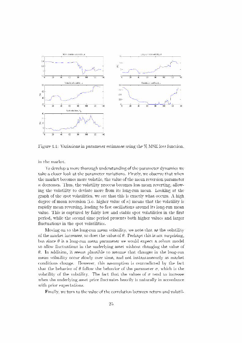
Figure 4.1: Variations in parameter estimates using the % MSE loss function.
in the market.
To develop a more thorough understanding of the parameter dynamics wetake a closer look at the parameter variations. Firstly, we observe that whenthe market becomes more volatile, the value of the mean reversion parameterκ decreases. Thus, the volatility process becomes less mean reverting, allow-ing the volatility to deviate more from its long-run mean. Looking at thegraph of the spot volatilities, we see that this is exactly what occurs. A highdegree of mean reversion (i.e. higher value of κ) means that the volatility israpidly mean reverting, leading to fast oscillations around its long-run meanvalue. This is captured by fairly low and stable spot volatilities in the �rstperiod, while the second time period presents both higher values and larger�uctuations in the spot volatilities.
Moving on to the long-run mean volatility, we note that as the volatilityof the market increases, so does the value of θ. Perhaps this is not surprising,but since θ is a long-run mean parameter we would expect a robust modelto allow �uctuations in the underlying asset without changing the value ofθ. In addition, it seems plausible to assume that changes in the long-runmean volatility occur slowly over time, and not instantaneously as marketconditions change. However, this assumption is contradicted by the factthat the behavior of θ follow the behavior of the parameter σ, which is thevolatility of the volatility. The fact that the values of σ tend to increasewhen the underlying asset price �uctuates heavily is naturally in accordancewith prior expectations.
Finally, we turn to the value of the correlation between return and volatil-
25

ity. Having noted earlier that the value of ρ a�ects the skewness distribution,we would expect the correlation coe�cient to become more negative whenmarkets are volatile. Looking at the graph of ρ we note that the actualoutcome is in line with our expectations. When the underlying asset price�uctuate the value of ρ decreases, thus creating a fat left-tailed distribution.All in all, the Heston model is consistent in the sense that the parametervariations can be readily explained by the current market conditions.
Figure 4.2: Variations in parameter estimates using the $ MSE loss function.
Figure 4.3: Variations in parameter estimates using the IV MSE loss func-tion.
If we brie�y consider the variations of the parameter estimates from the$ MSE function and the IV MSE function (see �gures 4.2 and 4.3) we note
26

that the patterns are very similar. This indicates that the time inconsistencypresent in the Heston model is not due to the calibration method, but ratheran inherent feature of the model. In the next section, we look closer at therobustness of the Dupire model, and in particular the results obtained fromthe principal component analysis.
4.2 The Dupire Model
Unlike the Heston model, where there are a large number of papers on the cal-ibration process, the calibration of the Dupire model required several steps oftrial and error. Since the implicit method is known to give more stable solu-tions, the explicit method was never implemented in practice. Furthermore,the $ MSE loss function was used during the calibrations. The appropriatevalues of the regularization parameters αK and αT were also determinedusing trial and error. It turns out that for the given market data αK = 107
and αT = 10 give good prices and su�ciently smooth volatility surfaces.The large di�erence between the two parameters is simply due to the factthat the value of the second derivative with respect to K is in general muchsmaller than the corresponding second derivative with respect to T . Thee�ects of adding the regularization terms are illustrated in �gures 4.4 and4.5 below.
Figure 4.4: Local volatility function on June 23rd when no regularizationterm is added.
27

Figure 4.5: Local volatility function on June 23rd when a regularization termis added.
Care should be taken not to confuse the local volatilies with impliedvolatilities. However, the two are closely connected. Gatheral (2006) showsthat there is a quite intuitive picture for the meaning of Black-Scholes im-plied variance of a European option with a given strike and expiration: It isapproximately the integral from today to expiration of local variances alongthe most probable path for the stock price conditional on the stock price atexpiration being the strike price of the option. This mental picture shouldbe kept in mind as we analyse the dynamics of the local volatility function.
Moving on to the variation of the local volatility function over time, wenote that in accordance with the Heston model, there are two distinct timeperiods where the properties of the model vary signi�cantly. During the �rstperiod (�rst 60 days), when the price of the underlying asset is quite stable,the shape of the volatility surface is fairly constant. We also note that themodel is able to capture the volatility smirk that has been readily observedin the market. The volatility function is also fairly stable with respect to thetime to maturity, which is in line with prior expectations.
In the second period, when the �uctuations in the market increase inamplitude, the shape of the volatility surface is heavily distorted (see �gure4.7), with out-of-the-money volatilities approaching zero. Essentially, thisis equivalent to saying that the market's expectations of a rise in the priceof underlying are very low. Consequently, the prices of out-of-the-money
28

Figure 4.6: Local volatility function on September 11th
calls will drop as well as the corresponding volatilities. Moreover, the factthat the shape of the local volatility function varies considerably over time,provides a �rst indicator of time inconsistency in the Dupire model.
A more thorough understanding of the underlying dynamics of the volatil-ity surface is provided by the principal component analysis. The Matlabfunction princomp was used to calculate the principal components of thesurface variations, and the cumulative variances of the �rst six componentsare shown in table 4.2 below. Consequently, we establish that the three �rst
Table 4.2: Cumulative variances of the �rst six principal components.
Principal component Cumulative variance
1 0.446292 0.80023 0.888214 0.940175 0.967036 0.98439
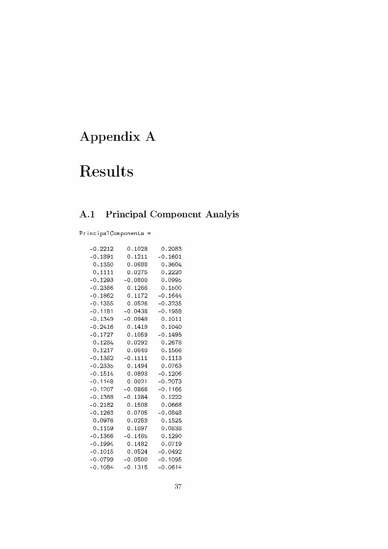
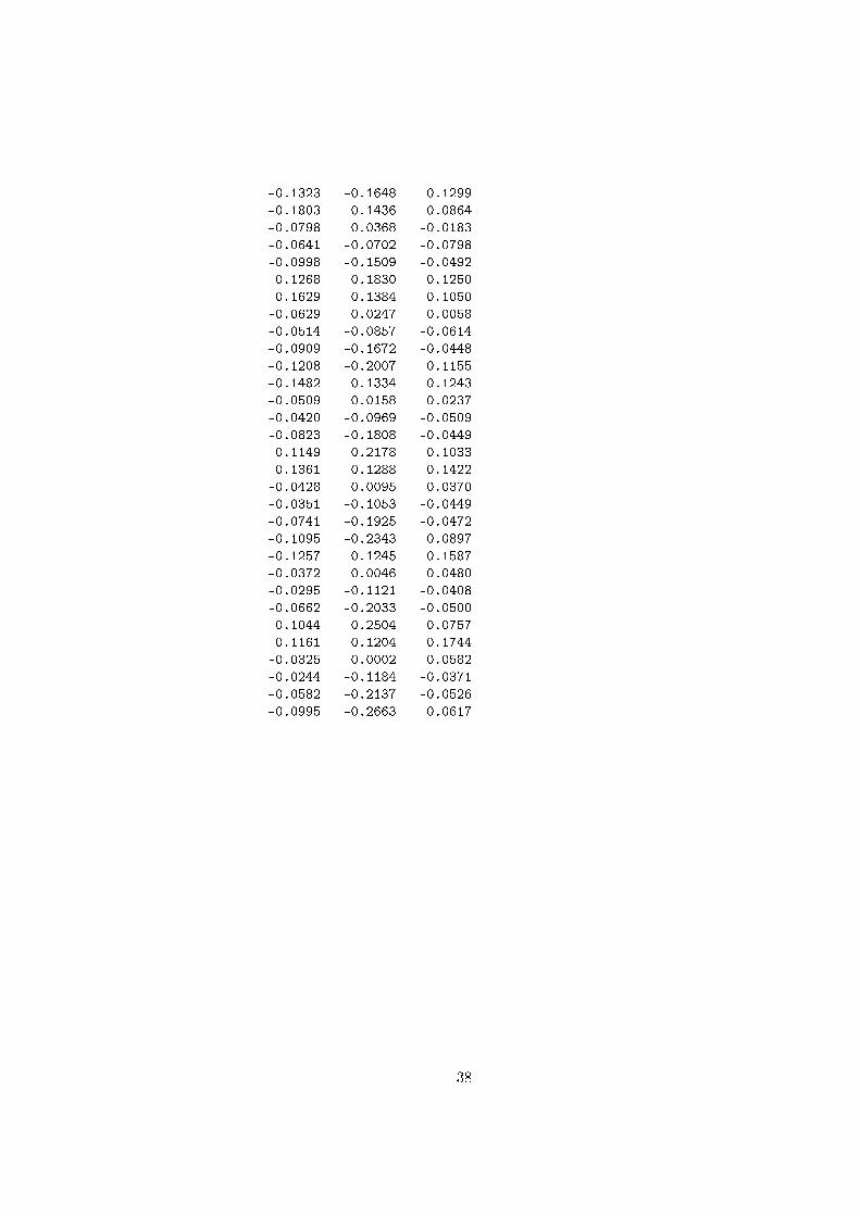
principal components account for almost 90 % of the total variance in thelocal volatility function. A closer look at these principal components (seeAppendix A) reveals that the variance of the volatility surface to a large
29
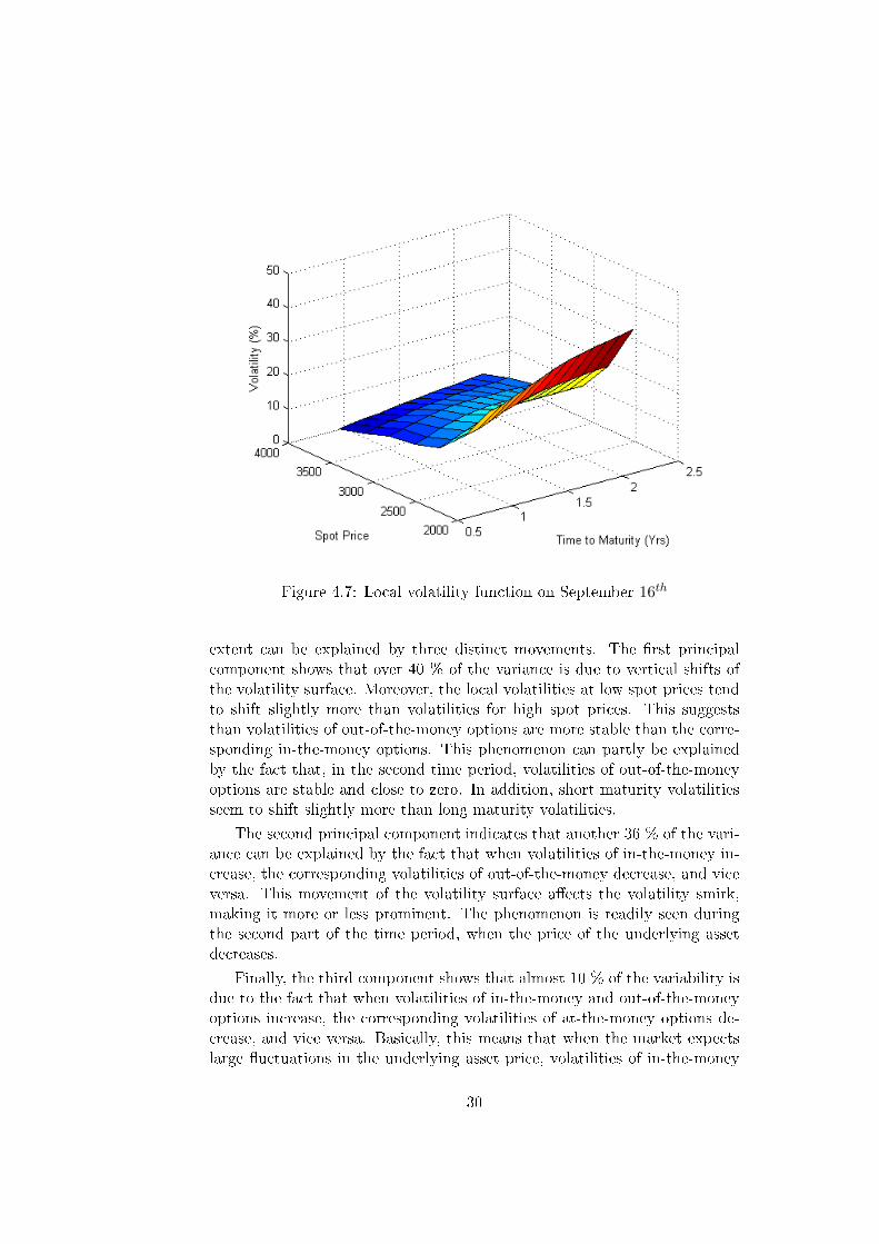
Figure 4.7: Local volatility function on September 16th
extent can be explained by three distinct movements. The �rst principalcomponent shows that over 40 % of the variance is due to vertical shifts ofthe volatility surface. Moreover, the local volatilities at low spot prices tendto shift slightly more than volatilities for high spot prices. This suggeststhan volatilities of out-of-the-money options are more stable than the corre-sponding in-the-money options. This phenomenon can partly be explainedby the fact that, in the second time period, volatilities of out-of-the-moneyoptions are stable and close to zero. In addition, short maturity volatilitiesseem to shift slightly more than long maturity volatilities.
The second principal component indicates that another 36 % of the vari-ance can be explained by the fact that when volatilities of in-the-money in-crease, the corresponding volatilities of out-of-the-money decrease, and viceversa. This movement of the volatility surface a�ects the volatility smirk,making it more or less prominent. The phenomenon is readily seen duringthe second part of the time period, when the price of the underlying assetdecreases.
Finally, the third component shows that almost 10 % of the variability isdue to the fact that when volatilities of in-the-money and out-of-the-moneyoptions increase, the corresponding volatilities of at-the-money options de-crease, and vice versa. Basically, this means that when the market expectslarge �uctuations in the underlying asset price, volatilities of in-the-money
30

and out-of-the-money options will increase as the corresponding option pricesgo up. In a volatile market, the demand for at-the-money options is likelyto decrease, thus leading to a reduction of at-the-money volatilities.
So, in accordance with the results obtained from the Heston model, theDupire model is robust in the sense that the observed surface variationscan be readily explained by the underlying asset and the current marketconditions. On the other hand, the model shows a high degree of timeinconsistency, as the shape of the local volatility function tends to �uctuateheavily when the market is volatile. Moreover, the principal componentanalysis turns out to be an extremely useful tool in reducing the noise inparameter variations and explaining, in a self-consistent way, the dynamicsof the Dupire model.
31

32

Chapter 5
Conclusions
This paper investigates the time consistency of two structural option pricingmodels, in terms of variations in daily parameter estimates. Our resultsshow that the parameter variations can be readily explained by the currentmarket conditions, while the fact that they vary indicate an inherent timeinconsistency of the models. This is interesting for several reasons.
The models investigated are constructed based on the assumption thatthe long-term evolution of the underlying spot price and its volatility canbe described using suitable di�usion processes. At some time t we calibratethe models to market data, expecting to �nd parameters that are consistentwith the market's expectations of the future evolution of the underlying assetprice, in the sense that they are able to recover option prices as accurately aspossible. In a time consistent model, these parameter estimates completelyspecify the set of possible structures for any t > 0. Since the parameterestimates vary over time, we conclude that the main assumptions of trueunderlying di�usion processes are inaccurate, partly agreeing with earlierresearch conducted by for example Christo�ersen and Jacobs (2004).
In summary, this thesis provides valuable insights regarding the dynamicsof current option pricing models. At the same time, the inconsistenciesarising from the varying parameter estimates, as well as the di�culties incalibrating the models, shows that much of the option pricing theory is yetto be discovered, both regarding model speci�cation and implementation.
33

34
Bibliography
[1] Bakshi, G., Cao, Charles., and Chen, Z. 1997. Empirical Performanceof Alternative Option Pricing Models. The Journal of Finance 52, 2003- 2049.
[2] Björk, T., Arbitrate Theory in Continuous Time. Oxford UniversityPress, New York, 2 edition, 2004.
[3] Black, F., and Scholes, M. 1973. The Pricing of Options and CorporateLiabilities. Journal of Political Economy 81, 653 - 659.
[4] Brecher, D. 2006. Pushing the Limits of Local Volatility in OptionPricing. Wilmott Magazine, pp. 6 - 15.
[5] Carr, P., and Madan, D. 1999. Option valuation using the Fast FourierTransform.
[6] Christo�ersen, P., Heston, S., and Jacobs, K. 2009. The shape andterm structure of the index option smirk: Why multifactor stochasticvolatility models work so well.
[7] Christo�ersen, P., Jacobs, K., The Importance of the Loss Function
in Option Valuation, Journal of Financial Economics 2004 Volume 72,pp. 291 - 318
[8] Cont, R., and Hamida, S. 2005. Recovering volatility from option pricesby evolutionary algorithm. Journal of Computational Finance 8.
[9] Cox, John C., Jonathan E. Ingersoll, and Steven A. Ross. 1985. Atheory of the term structure of interest rates. Econometrica 53, 385 -407.
[10] Cox, John C., and Ross, Stephen A. 1976, The Valuation of Options
for Alternative Stochastic Processes, Journal of Financial Economics8, 43 - 76.
[11] Derman, E., and Kani, I. 1994. Riding on a Smile. Risk 7, 32 - 39.
[12] Detlefsen, K., Härdle, W., Discussion Paper, 2006
35
[13] Dupire, B. 1993. Pricing and Hedging with a Smile.
[14] Dupire, B. 1994. Pricing with a Smile. Risk 7, 18 - 20.
[15] Elder, John. 2002. Hedging for �nancial derivatives. University of Ox-
ford. Ph.D. Thesis.
[16] Feller, W. 1951. Two singular di�usion problems. The Annals of Math-
ematics 54, 173-182.
[17] Gatheral, J., The Volatility Surface - A Practitioners Guide, John Wi-ley & Sons, Inc.
[18] Hamida, C., Cont, R.,Recovering Volatility from Option Prices by Evo-
lutionary Optimization
[19] Heston S. 1993. A closed-form solution for options with stochasticvolatility, with application to bond and currency options. Review of
Financial Studies 6, 327 - 343.
[20] Mikhailov, S., and Nögel, U. 2003. Heston's stochastic volatility model,calibration and some extensions. Wilmott Magazine, pp. 74 - 79.
[21] Schoutens, Wim., Simons, Erwin., and Tistaert, Jurgen. 2003. A Per-fect Calibration! Now What?
36
Appendix A
Results
A.1 Principal Component Analyis
PrincipalComponents =
-0.2212 0.1028 0.2083
-0.1891 0.1211 -0.1601
-0.1350 0.0688 -0.3604
-0.1111 -0.0275 -0.2220
-0.1293 -0.0800 0.0995
-0.2386 0.1266 0.1500
-0.1862 0.1172 -0.1644
-0.1355 0.0526 -0.3235
-0.1181 -0.0438 -0.1958
-0.1349 -0.0949 0.1011
-0.2416 0.1419 0.1040
-0.1727 0.1059 -0.1495
-0.1284 0.0292 -0.2678
-0.1217 -0.0640 -0.1566
-0.1382 -0.1111 0.1113
-0.2335 0.1494 0.0763
-0.1514 0.0893 -0.1206
-0.1148 0.0021 -0.2073
-0.1207 -0.0866 -0.1166
-0.1388 -0.1284 0.1222
-0.2182 0.1508 0.0668
-0.1263 0.0705 -0.0848
-0.0976 -0.0253 -0.1525
-0.1159 -0.1097 -0.0838
-0.1366 -0.1465 0.1290
-0.1994 0.1482 0.0719
-0.1015 0.0524 -0.0492
-0.0799 -0.0500 -0.1095
-0.1084 -0.1315 -0.0614
37
-0.1323 -0.1648 0.1299
-0.1803 0.1436 0.0864
-0.0798 0.0368 -0.0183
-0.0641 -0.0702 -0.0798
-0.0998 -0.1509 -0.0492
-0.1268 -0.1830 0.1250
-0.1629 0.1384 0.1050
-0.0629 0.0247 0.0058
-0.0514 -0.0857 -0.0614
-0.0909 -0.1672 -0.0448
-0.1208 -0.2007 0.1155
-0.1482 0.1334 0.1243
-0.0509 0.0158 0.0237
-0.0420 -0.0969 -0.0509
-0.0823 -0.1808 -0.0449
-0.1149 -0.2178 0.1033
-0.1361 0.1288 0.1422
-0.0428 0.0095 0.0370
-0.0351 -0.1053 -0.0449
-0.0741 -0.1925 -0.0472
-0.1095 -0.2343 0.0897
-0.1257 0.1245 0.1587
-0.0372 0.0046 0.0480
-0.0295 -0.1121 -0.0408
-0.0662 -0.2033 -0.0500
-0.1044 -0.2504 0.0757
-0.1161 0.1204 0.1744
-0.0325 0.0002 0.0582
-0.0244 -0.1184 -0.0371
-0.0582 -0.2137 -0.0526
-0.0995 -0.2663 0.0617
38

Appendix B
Matlab code
B.1 Calibrating the Heston model using Di�er-
ential Evolution
%%HestonDECalibration uses a Differential Evolution Algorithm to fit the
%%parameters of the Heston model to market option prices.
%%The optimization scheme can be downloaded from
%%http://www.mathworks.com/matlabcentral/fileexchange/18593
clear, close all
clc
global OptionData; global NoOfOptions; global PriceDifference;
global ImplBSVol; global InitialParameters;
load RawOptionData.m; %% r - D, T, S0, K, C, r, D
%CALCULATE THE NUMBER OF DATES AND THE NUMBER OF OPTIONS FOR EACH DATE
[B,I,J] = unique(RawOptionData(:,3),'first');
Index = sort(I); Index(length(Index) + 1) = length(RawOptionData(:,3));
for i=1:length(Index)-1
NoOptions(i) = Index(i+1)-Index(i);
end
NoOptions(length(NoOptions)) = NoOptions(length(NoOptions))+1;
NoOfDates = length(NoOptions);
NUsed = 1;
%SET INITIAL PARAMETERS: [Kappa;Theta;Sigma;Rho;V0]
InitialParameters = [2.3846;0.02522;0.33714;-0.64819;0.09163];
Results = [];
for j=1:NoOfDates
39

NoOfOptions = NoOptions(j);
OptionData = RawOptionData([NUsed:NUsed+NoOfOptions-1],:);
%%IF WE USE THE IV MSE LOSS FUNCTION, CALCULATE THE IMPLIED
%%BLACK-SCHOLES VEGA: OTHERWISE, THIS SECTION MAY BE
%%IGNORED
%for k=1:NoOfOptions
%y = OptionData(k,:);
%ImplBSVol(k) = fzero(@(x) bsvolatility(x,y),0.2);
%end
%for l=1:NoOfOptions
%OptionData(l,8) = blsvega(OptionData(l,3),OptionData(l,4),...,
%OptionData(l,6),OptionData(l,2),ImplBSVol(l),OptionData(l,7));
%end
%SPECIFY PARAMETERS FOR THE DIFFERENTIAL EVOLUTION OPTIMIZATION
optimInfo.title = 'Heston Differential Evolution Calibration';
objFctHandle = @HestonCostFunc;
paramDefCell = {'',[0.5 7;0.001 1;0.001 1;-1 1;0.001 0.5],...,
[1e-5*ones(5,1)],InitialParameters};
objFctSettings = {};
objFctParams = [];
DEParams = getdefaultparams;
DEParams.NP = 100;
DEParams.feedSlaveProc = 0;
DEParams.validChkHandle = @HestonConstraint; %2*Kappa*Theta>=0
DEParams.maxiter = 1e5;
DEParams.maxtime = 600; %Maximum optimization time (in secs)
DEParams.maxclock = [];
DEParams.refreshiter = 1;
DEParams.refreshtime = 10;
DEParams.refreshtime2 = 600;
DEParams.refreshtime3 = 1200;
emailParams = [];
rand('state',1);
%bestmem = PARAMETER ESTIMATES, bestval = LOSS FUNCTION VALUE
[bestmem,bestval] = differentialevolution(DEParams,paramDefCell,...,
objFctHandle,objFctSettings,objFctParams,emailParams,optimInfo);
NUsed = NUsed + NoOfOptions;
InitialParameters = bestmem;
Results = [Results;bestmem' bestval];
end
40

function val = HestonCostFunc(x, noPause)
global OptionData;
global NoOfOptions;
global PriceDifference;
global ImplBSVol;
global InitialParameters;
%% CHOOSE THE LOSS FUNCTION TO BE USED AND THE REGULARIZATION PARAMETER
%% IV-MSE LOSS FUNCTION
% for i = 1:NoOfOptions
% PriceDifference(i) = (OptionData(i,5) - ...,
% HestonCallQuad(x(1),x(2),x(3),x(4),x(5),OptionData(i,1),...,
% OptionData(i,2),OptionData(i,3),OptionData(i,4)))/...,
% ((blsvega(OptionData(i,3),OptionData(i,4),OptionData(i,6),...,
% OptionData(i,2),ImplBSVol(i),OptionData(i,7))));
% end
% RegularizationParameter = 1;
% val = sqrt(1/NoOfOptions^2*sum(PriceDifference.^2)) + ...,
% RegularizationParameter*sum((InitialParameters-x).^2);
%% $-MSE LOSS FUNCTION
% for i = 1:NoOfOptions
% PriceDifference(i) = (OptionData(i,5) - ...,
% HestonCallQuad(x(1),x(2),x(3),x(4),x(5),OptionData(i,1),...,
% OptionData(i,2),OptionData(i,3),OptionData(i,4)));
% end
% RegularizationParameter = 1;
% val = sqrt(1/NoOfOptions^2*sum(PriceDifference.^2)) + ...,
% RegularizationParameter*sum((InitialParameters-x).^2);
%% %-MSE LOSS FUNCTION
for i = 1:NoOfOptions
PriceDifference(i) = (OptionData(i,5) - ...,
HestonCallPrice(x(1),x(2),x(3),x(4),x(5),OptionData(i,1),...,
OptionData(i,2),OptionData(i,3),OptionData(i,4)))/OptionData(i,5);
end
RegularizationParameter = 1;
val = sqrt(1/NoOfOptions^2*sum(PriceDifference.^2)) + ...,
RegularizationParameter*sum((InitialParameters-x).^2);
function call = HestonCallPrice(kappa,theta,sigma,rho,v0,r,T,s0,K)
warning off;
call = s0*HestonProbabilities(kappa,theta,sigma,rho,v0,r,T,s0,K,1)- ...,
K*exp(-r*T)*HestonProbabilities(kappa,theta,sigma,rho,v0,r,T,s0,K,2);
41

function ret = HestonProbabilities(kappa,theta,sigma,rho,v0,r,T,s0,K,type)
ret = 0.5 + 1/pi*quadl(@HestonIntegrand,0,100,[],[],kappa,theta,sigma,...,
rho,v0,r,T,s0,K,type);
function ret = HestonIntegrand(phi,kappa,theta,sigma,rho,v0,r,T,s0,K,type)
ret = real(exp(-i*phi*log(K)).*HestonCharFunc(phi,kappa,theta,sigma,...,
rho,v0,r,T,s0,type)./(i*phi));
function f = HestonCharFunc(phi,kappa,theta,sigma,rho,v0,r,T,s0,type);
if type == 1
u = 0.5;
b = kappa - rho*sigma;
else
u = -0.5;
b = kappa;
end
a = kappa*theta;
x = log(s0);
d = sqrt((rho*sigma*phi.*i-b).^2 - sigma^2*(2*u*phi.*i-phi.^2));
g = (b - rho*sigma*phi*i + d)./(b - rho*sigma*phi*i - d);
C = r*phi.*i*T + a/sigma^2.*((b - rho*sigma*phi*i + d)*T - ...,
2*log((1-g.*exp(d*T))./(1-g)));
D = (b - rho*sigma*phi*i + d)./sigma^2.*((1-exp(d*T))./(1-g.*exp(d*T)));
f = exp(C + D*v0 + i*phi*x);
B.2 Calibrating the Heston model using
lsqnonlin
clear, close all
clc
global NoOfOptions; global OptionData;
global InitialParameters;
load RawOptionData.m; %% r - D, T, S0, K, C, r, D
%CALCULATE THE NUMBER OF DATES AND THE NUMBER OF OPTIONS FOR EACH DATE
[B,I,J] = unique(RawOptionData(:,3),'first');
Index = sort(I); Index(length(Index) + 1) = length(RawOptionData(:,3));
42

for i=1:length(Index)-1
NoOptions(i) = Index(i+1)-Index(i);
end
NoOptions(length(NoOptions)) = NoOptions(length(NoOptions))+1;
NoOfDates = length(NoOptions);
NUsed = 1;
%SET INITIAL PARAMETERS: [Kappa;Theta;Sigma;Rho;V0]
InitialParameters = [2.3846;0.02522;0.33714;-0.64819;0.09163];
Results = [];
for j=1:NoOfDates
NoOfOptions = NoOptions(j);
OptionData = RawOptionData([NUsed:NUsed+NoOfOptions-1],:);
%%IF WE USE THE IV MSE LOSS FUNCTION, CALCULATE THE IMPLIED
%%BLACK-SCHOLES VEGA: OTHERWISE, THIS SECTION MAY BE
%%IGNORED
%for k=1:NoOfOptions
%y = OptionData(k,:);
%ImplBSVol(k) = fzero(@(x) bsvolatility(x,y),0.2);
%end
%for l=1:NoOfOptions
%OptionData(l,8) = blsvega(OptionData(l,3),OptionData(l,4),...,
%OptionData(l,6),OptionData(l,2),ImplBSVol(l),OptionData(l,7));
%end
bestmem = lsqnonlin(@(x) HestonDifferences(x),...,
InitialParameters,[0.5 7;0.001 1;0.001 1;-1 1;0.001 0.5]);
Results = [Results;bestmem'];
NUsed = NUsed + NoOfOptions;
InitialParameters = bestmem;
end
function ret = HestonDifferences(x)
global NoOfOptions; global OptionData;
global InitialParameters;
%% CHOOSE THE LOSS FUNCTION TO BE USED AND THE REGULARIZATION PARAMETER
%% IV-MSE LOSS FUNCTION
% for i = 1:NoOfOptions
% PriceDifference(i) = (OptionData(i,5) - ...,
% HestonCallQuad(x(1),x(2),x(3),x(4),x(5),OptionData(i,1),...,
% OptionData(i,2),OptionData(i,3),OptionData(i,4)))/...,
% ((blsvega(OptionData(i,3),OptionData(i,4),OptionData(i,6),...,
% OptionData(i,2),ImplBSVol(i),OptionData(i,7))));
% end
43

% RegularizationParameter = 1;
% for j=1:5
% PriceDifference(NoOfOptions+j) = sqrt(RegularizationParameter)*...
%(InitialParameters(j)-x(j));
% end
% ret = PriceDifference;
%% $-MSE LOSS FUNCTION
% for i = 1:NoOfOptions
% PriceDifference(i) = (OptionData(i,5) - ...,
% HestonCallQuad(x(1),x(2),x(3),x(4),x(5),OptionData(i,1),...,
% OptionData(i,2),OptionData(i,3),OptionData(i,4)));
% end
% RegularizationParameter = 1;
% for j=1:5
% PriceDifference(NoOfOptions+j) = sqrt(RegularizationParameter)*...
%(InitialParameters(j)-x(j));
% end
% ret = PriceDifference;
%% %-MSE LOSS FUNCTION
for i = 1:NoOfOptions
PriceDifference(i) = (OptionData(i,5) - ...,
HestonCallPrice(x(1),x(2),x(3),x(4),x(5),OptionData(i,1),...,
OptionData(i,2),OptionData(i,3),OptionData(i,4)))/OptionData(i,5);
end
RegularizationParameter = 1;
for j=1:5
PriceDifference(NoOfOptions+j) = sqrt(RegularizationParameter)*...
(InitialParameters(j)-x(j));
end
ret = PriceDifference;
B.3 Calibrating the Dupire model using
lsqnonlin
clear, close all
clc
global S0; global K; global NPartition; global dT; global dK;
global u; global AlphaK; global AlphaT; global CallObservations;
load RawOptionData.m;
[B,I,J] = unique(RawOptionData(:,3),'first');
Index = sort(I); Index(length(Index) + 1) = length(RawOptionData(:,3));
for i = 1:length(Index)-1
44

NoOfOptions(i) = Index(i+1)-Index(i);
end
NoOfOptions(length(NoOfOptions)) = NoOfOptions(length(NoOfOptions)) + 1;
NoOfDates = length(NoOfOptions); NUsed = 1;
NPartition = 20;
InitialVol = 0.2*ones(NPartition-1,NPartition-2); %INITIAL PARAMETERS
Results = []; TVec = []; KVec = [];
AlphaK = 10^7; AlphaT = 10;
for i=1:NoOfDates
OptionData = RawOptionData([NUsed:NUsed+NoOfOptions(i)-1],:);
S0 = OptionData(1,3);
Tmin = min(OptionData(:,2)); Tmax = max(OptionData(:,2));
dT = Tmax/(NPartition-1); T = 0:dT:Tmax;
Kmin = 0; Kmax = 2*S0; %Note that the value of Kmax may vary between
dK = Kmax/(NPartition-1);%different dates. Choose Kmax sufficiently
K = 0:dK:Kmax; %large, so that we may set the value of
%options with K = Kmax to 0.
t1 = OptionData(:,2); k1 = OptionData(:,4); c1 = OptionData(:,5);
TUnique = unique(t1); KUnique = unique(k1);
k2 = zeros(length(TUnique),1); k3 = Kmax*ones(length(TUnique),1);
tk_initial = [t1 k1 c1;
TUnique k2 S0*ones(length(TUnique),1);
TUnique k3 zeros(length(TUnique),1)];
tk = tk_initial(:,[1:2]); c = tk_initial(:,3);
calls = tpaps(tk',c');
for j=1:length(T)
for k=1:length(K)
CallObservations(j,k) = max(fnval(calls,[T(j);K(k)]),0);
end
end
r_D = [OptionData(:,2) OptionData(:,1)];
rates = sortrows(unique(r_D,'rows'));
u = interp1(rates(:,1),rates(:,2),T,'pchip');
LVFunc = lsqnonlin(@(v) ImplicitDupire(v),InitialVol,zeros(NPartition-1,...
,NPartition-2),ones(NPartition-1,NPartition-2));
Results = [Results;LVFunc]; TVec = [TVec;T]; KVec = [KVec;K];
InitialVol = LVFunc;
NUsed = NUsed + NoOfOptions(i);
end
45
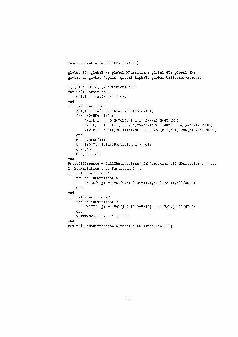
function ret = ImplicitDupire(Vol)
global S0; global K; global NPartition; global dT; global dK;
global u; global AlphaK; global AlphaT; global CallObservations;
C(1,1) = S0; C(1,NPartition) = 0;
for i=2:NPartition-1
C(1,i) = max(S0-K(i),0);
end
for t=2:NPartition
A(1,1)=1; A(NPartition,NPartition)=1;
for k=2:NPartition-1
A(k,k-1) = -0.5*Vol(t-1,k-1)^2*K(k)^2*dT/dK^2;
A(k,k) = 1 + Vol(t-1,k-1)^2*K(k)^2*dT/dK^2 - u(t)*K(k)*dT/dK;
A(k,k+1) = u(t)*K(k)*dT/dK - 0.5*Vol(t-1,k-1)^2*K(k)^2*dT/dK^2;
end
B = sparse(A);
b = [S0;C(t-1,[2:NPartition-1])';0];
c = B\b;
C(t,:) = c';
end
PriceDifference = CallObservations([2:NPartition],[2:NPartition-1])-...
C([2:NPartition],[2:NPartition-1]);
for i=1:NPartition-1
for j=1:NPartition-4
VolKK(i,j) = (Vol(i,j+2)-2*Vol(i,j+1)+Vol(i,j))/dK^2;
end
end
for i=1:NPartition-2
for j=1:NPartition-3
VolTT(i,j) = (Vol(j+2,i)-2*Vol(j+1,i)+Vol(j,i))/dT^2;
end
VolTT(NPartition-1,:) = 0;
end
ret = [PriceDifference AlphaK*VolKK AlphaT*VolTT];
46