time-based competition in multistage manufacturing:...

The International Journal of Flexible Manufacturing Systems, 16, 11–44, 2004c© 2004 Kluwer Academic Publishers. Manufactured in The Netherlands.

Time-Based Competition in Multistage Manufacturing:Stream-of-Variation Analysis (SOVA)Methodology—Review

D. CEGLAREK [email protected]. HUANG [email protected]. ZHOU [email protected] of Industrial Engineering, University of Wisconsin-Madison, Madison, WI 53706-1572, USA

Y. DING [email protected] of Industrial Engineering, Texas A&M University, College Station, TX 77843, USA

R. KUMAR [email protected]. ZHOU [email protected] Control Systems, Inc., Troy, MI 48084, USA

Abstract. Frequency of model change and the vast amounts of time and cost required to make a changeover,also called time-based competition, has become a characteristic feature of modern manufacturing and new productdevelopment in automotive, aerospace, and other industries. This paper discusses the concept of time-based com-petition in manufacturing and design based on a review of on-going research related to stream-of-variation (SOVAor SoV) methodology. The SOVA methodology focuses on the development of modeling, analysis, and controlof dimensional variation in complex multistage assembly processes (MAP) such as the automotive, aerospace,appliance, and electronics industries. The presented methodology can help in eliminating costly trial-and-errorfine-tuning of new-product assembly processes attributable to unforeseen dimensional errors throughout the as-sembly process from design through ramp-up and production. Implemented during the product design phase, themethod will produce math-based predictions of potential downstream assembly problems, based on evaluationsof the design and a large array of process variables. By integrating product and process design in a pre-productionsimulation, SOVA can head off individual assembly errors that contribute to an accumulating set of dimensionalvariations, which ultimately result in out-of-tolerance parts and products. Once in the ramp-up stage of produc-tion, SOVA will be able to compare predicted misalignments with actual measurements to determine the degreeof mismatch in the assemblies, diagnose the root causes of errors, isolate the sources from other assembly steps,and then, on the basis of the SOVA model and product measurements, recommend solutions.

Key Words: variation reduction, quality, root cause identification, manufacturing systems

1. Introduction: Time-based-competition—New paradigm and challenges

The US automotive industry has dominated world auto markets for years. The mass produc-tion paradigm, initiated by Henry Ford and Frederick W. Taylor, has been the most powerfultool for the United States in global markets for almost half of the last century. However,the landscape has shifted dramatically from the old world of mass production, which wascharacterized by few standardized products, homogeneous markets, and long product life

12 CEGLAREK ET AL.

cycle and development lead time. A new standard is gradually emerging in which increasedcustomization, product proliferation, heterogeneous markets, shorter product life cycle anddevelopment time, responsiveness, and related factors are increasingly becoming key fea-tures (Bollinger, 1998; Gervin and Barrowman, 2002). For example, in Japan, Toyota wasreportedly offering customers five-day delivery from the time the customer designed acustomized car on a CAD system (from modular options) to the actual product delivery.

One of the characteristic features of the automotive industry is the frequency of modelchange and vast amounts of time and cost that are required to make a changeover. Thistrend has continuously gone up in the last two decades. Since 1980s, US car market’s totaldemand has essentially remained stable, but the number of nameplates has increased by35% from 139 to 183, respectively. This increase continued during the 1990s essentiallycreating a paradigm shift in automotive industry.

The newly emerging manufacturing paradigm is characterized by the so-called time-based-competition (TBC). The time to market for a new product or the service responsive-ness of a company has become the new cutting edge in global market competition (Ulrich,Sartorius, Pearson, and Jakiela, 1993). The major advantages of this new strategy are widelyrecognized to be (1) use of a newer technology than competitors in a newly developed prod-uct (2) capturing new market niche earlier than that of a competitor (3) higher customersatisfaction, and (4) better integration of the entire enterprise. In addition, it is possible thatthe company will parallelly achieve higher quality, lower cost, and a leaner organization(Suri, 1998).

In order to support as well as take full advantage of the aforementioned TBC strategies,new techniques such as quick response manufacturing (Suri, 1998), reconfigurable manu-facturing system (Koren et al., 1999; Mehrabi, Ulsoy, and Koren, 2000), agile manufacturingetc. have been proposed, developed, and applied in the last decade.

1.1. Challenges in automotive industry

Due to rapid changes in market demands in recent years, shortened product cycle is in-evitably becoming the prevailing trend. For example, in the automotive industry, a productlife cycle will be shortened to 2–3 years in a few years as compared to the current 4–7 yearsand 9–12 years from a few years ago. Additionally, market requirements demand signifi-cantly shorter new product realization cycles. Currently, it takes 24 months for the world’stop auto manufacturers to develop a new car, with development time expected to be reducedto 12–18 months within the next five years. Similar trends are also apparent in the appli-ance and consumer good industries. As a result, there are a number of new concepts in thearea of production system development, such as flexible and reconfigurable manufacturingsystems (RMS) and quick response manufacturing (QRM), which are increasingly beingadopted in industrial practices. However, due to lack of confidence in predicting systemperformance (ramp-up time, expected yield, and relatively long time necessary to reach it),there is tremendous resistance to implement advanced technology or innovations in newproduct/process development (CIRP, 2000).

The most significant obstacles toward reducing new product realization time stem fromthe complexity of the product/process and knowledge- or expertise-based product/process

TIME-BASED COMPETITION IN MULTISTAGE MANUFACTURING 13

development methods. They can be further categorized into (1) design phase: large numberof design/engineering changes that have to be made after the product has been designedand at times even after it has been built (6,000 changes on average for a new automotivebody development); (2) pre-production phase: long ramp up time, especially for complexsystems such as flexible machining transfer lines (up to 12–14 months), and automotiveassembly lines (3–5 months); (3) full production phase: low production yield (below designintent expectations: 65–70% for flexible machining line).

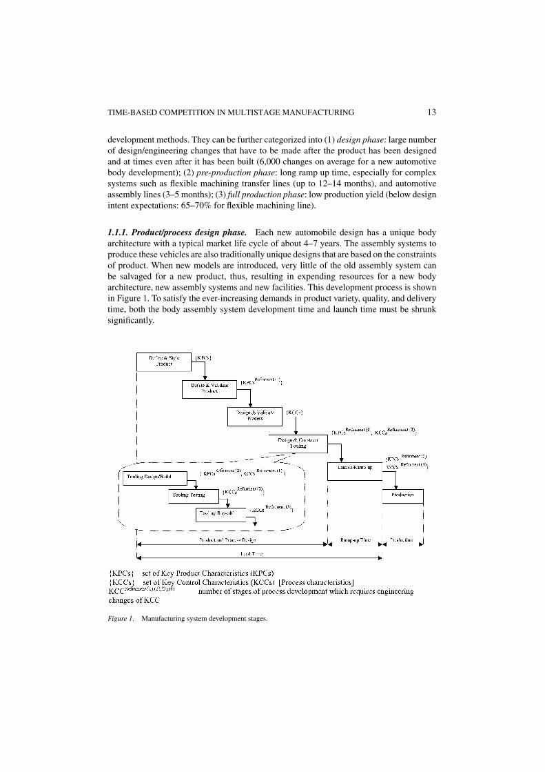
1.1.1. Product/process design phase. Each new automobile design has a unique bodyarchitecture with a typical market life cycle of about 4–7 years. The assembly systems toproduce these vehicles are also traditionally unique designs that are based on the constraintsof product. When new models are introduced, very little of the old assembly system canbe salvaged for a new product, thus, resulting in expending resources for a new bodyarchitecture, new assembly systems and new facilities. This development process is shownin Figure 1. To satisfy the ever-increasing demands in product variety, quality, and deliverytime, both the body assembly system development time and launch time must be shrunksignificantly.

Figure 1. Manufacturing system development stages.

14 CEGLAREK ET AL.

Product development time strongly depends on the ratio of “first time right” strategy,which tries to eliminate additional changes after the design phase.

For example, according to a 1999 survey conducted by the University of Michigan, itis estimated that some US automotive manufacturers reach 50–60% of “first time right”during design stage, as compared to 80% achieved by the top international competitor. Thiscauses significant barriers in realizing TBC manufacturing strategies in the overall productdevelopment cycle (Thomke and Fujimoto, 2000).

Additionally, it was reported that in aerospace and automotive industries 67–70% ofall design changes are related to product-dimensional variation (Shalon, Gossard, Ulrich,and Fitzpatrick, 1992; Ceglarek and Shi, 1995) caused by lack of technology for accurateprediction of process performance/variation during the product/process design. It is widelyrecognized that geometrical accuracy and dimensional variation are two of the most impor-tant quality and productivity factors in many manufacturing processes. In fact, dimensionalvariation is introduced into virtually every design when manufactured (Parkinson, Sorensen,and Pourhassan, 1993). Thus, the lack of a comprehensive technology for product/processperformance prediction and control is a major barrier to further progress in new product andprocess development. Moreover, the waste resulted from the aforementioned engineeringchanges done after the design phase can be translated into $84/vehicle for repair/rework(this does not include process change costs and overhead cost), lower production yield,and delay in starting production (higher product development cost, lost market share dueto delay in introduction of a new product, shorter production time—overall lower profits orhigher product costs).

1.1.2. Ramp-up for new production systems. New production ramp-up/launch time iscritical in new product manufacturing. The major efforts during ramp-up are focused onidentifying the root causes of process variation (Figure 2). However, current industrialpractice in ramp-up time reduction is far less than satisfactory. For example, in one USautomotive plant the designed production volume was reached near full after 14 months oflaunching a new vehicle assembly line. Most of the problems are related to dimensionalcontrol of product variation. In another plant, the design intended yield could not be main-tained due to dimensional variation of parts after 6 months of product launch (ERC-RMS,1999; Figure 3).

Although product and process design impact one another, product design has tradition-ally been separated from process design even in different companies, for example, toolingwherein dies, fixtures, material handling facilities etc. are usually designed and manufac-tured by different suppliers. Lately, manufacturers have begun to investigate ways to simul-taneously evaluate product designs and manufacturing processes in an attempt to eliminatedownstream problems of manufacturing (ramp-up time, yield etc.) (El-Gizawy, Hwang,and Brewer, 1990; Gadh, 1993). However, most of the design rules and guidelines requireexperience-based knowledge—there was no generic model, which could lead to compre-hensive technology to solve the aforementioned problems. Traditionally, design engineershave arrived at a product design configuration through use of engineering science principles.This often results in the designer specifying the target values for critical design parameters.


Figure 2. Dimensional fault root cause classification during ramp-up and full production (Ceglarek and Shi,1995).

Figure 3. New product/process development flow diagram (Koren et al., 1999).

16 CEGLAREK ET AL.

However, through this procedure, the specification limits are usually determined by thedesign engineer before the final product is released for production. This product-orientedapproach is referred to as over-the-wall design since there is no systematic integration ofdesign and manufacturing. This out-of-date design philosophy is one of the reasons whysome auto companies still have a lower first-time-right rate. A typical example is tolerancedesign.

Traditional tolerancing research (Chase and Parkinson, 1991) mainly focused on an as-sembly that is built up through numerous mating features of individual components. Inother words, the traditional tolerancing technique is primarily concerned with dimensionalor geometrical variables of a component in an assembly. Traditional tolerancing techniquescan be labeled as product-oriented tolerancing, since the explicit inclusion of process in-formation in the traditional tolerancing scenario is limited, where product variables andmanufacturing process are only weakly connected by the associated manufacturing cost.As long as the cost-tolerance function is specified, tolerance allocation can be conductedbased on the mathematical/functional model without considering any other effects fromthe manufacturing process. Recently, researchers have come to realize that the traditionalproduct-oriented approach overlooks the impact of process variables, such as informa-tion regarding fixture and tooling configuration, on product quality in complex multistagemanufacturing processes. The quality of the final product from a multistage manufacturingprocess is not only determined by the tolerance of each individual component but also af-fected by variations of numerous process variables such as fixturing error, force, and toolingvibration during different manufacturing stages. The term “process variable” covers a verybroad category and includes rather diverse number of parameters associated with manu-facturing process. They are not part of the product information but indicators of processstatus. One of the major challenges in analyzing process variables is that the relationshipbetween the variation of process variable and product quality is very complex, dependingon process design, tooling layout, and manufacturing sequence among others. Moreover,additional complexity is introduced because process variables can change over time dueto factors such as tooling degradation. Hence, they cannot be represented by simple worstcase or root square sum stack-up models or product functional model with only kinematicrelationship.

1.2. New Strategy: Introduction to stream-of-variation analysis (SOVA)

Manufacturers in the 21st century will face frequent and unpredictable market changes.These changes include rapid-frequency introduction of new products, increased demandfor new products and mix of products, new parts for existing products, and overall newprocess technologies. To gain the competitive advantage, manufacturing companies mustbe able to analyze, predict and optimize manufacturing system performance during thedesign phase (that is, do all design in the first time right “FTRDesign” approach) and be ableto identify and isolate root causes of all faults during ramp-up time (do all fault isolation inthe first time right “FTRDiagnosis” approach).

This leads to a new manufacturing strategy namely, math-based SOVA system workingin “FTRDesign/Diagnose” mode for product/process performance analysis. In the last decade,


Job 1

year

New ramp up Current ramp up

Lower variation start-point due to

FTR Design

Without SOVA

With SOVA

Short ramp-up due to FTR Diagnosis

Less downtime and defect during production

Var

iati

on L

evel

Job 1

year

Without SOVA

With SOVA

Num

ber

of e

ngin

eeri

ng

chan

ges

Most engineering changes incurred during design stage due to FTR

approach.

Process is quickly tuned to what-it-should-be due to prompt root

cause diagnosis

Newstart point

ov'

t0 t1

ov

cv

cv'

New ramp up Current ramp up

om

om'

cm

cm'

Root cause-based system performance

improvement

Process-oriented tolerancing

Figure 4. New product/process development criteria and requirements.

the so-called stream of variation analysis (SOVA) methodology has been proposed anddeveloped to overcome the aforementioned challenges (Ceglarek and Shi, 1994, 1995,1996; Apley and Shi, 1998; Hu, 1997; Ding, Ceglarek, and Shi, 2000, 2002a, 2002b; Ding,Shi, and Ceglarek, 2002c). SOVA is a generic math model for variation propagation analysisin multistage manufacturing systems. SOVA integrates multivariate statistics, control theoryas well as design/manufacturing knowledge (CAD/CAM models) into a unified framework.SOVA serves two objectives (Figure 4):

• In the design phase, the SOVA can be used for analysis, prediction, and optimizationof manufacturing system performance following the concept of “FTRDesign”. Given theprocess and tooling design information, SOVA can simulate the variation propagatingthroughout the process and then predict the final product-dimensional variation and re-sultant product geometry.

• In the production ramp-up phase, SOVA can be used to identify and isolate fault rootcauses following the concept of “FTRDiagnosis”. Given the process and tooling designinformation, SOVA can demonstrate high responsiveness in identifying and isolatingroot causes of dimensional variation, that is, identifying the most severe dimensionalfaults, localizing the critical stations contributing most to the final product variation andspeedily isolating the root causes of dimensional faults—achieving faster required V ′

clevel of variation as shown in Figures 4 and 5.

18 CEGLAREK ET AL.

Figure 5. Variation level comparative evaluation (Ceglarek and Shi, 1995; ERC-RMS, 1999).

Figure 6. Automotive body at the optical measurement station.

2. Background on automotive assembly process

Geometrical relations dominate assembly of the automotive body, shown in Figures 6 and 7,such that the quality of the assembly process can be determined by the dimensional integrityof a product. This indicates that the level of product-dimensional variation can be a criticalindex for final evaluation of the assembled vehicle.

2.1. Product and process

An automotive body is built from sheet metal parts, which have different shapes, sizes,and thickness, depending on their functions. These parts are categorized as structural ornonstructural. Structural parts support the automotive body structures and includes (1)main parts, such as rails and plenum, or (2) reinforcement parts, for instance, door hinge


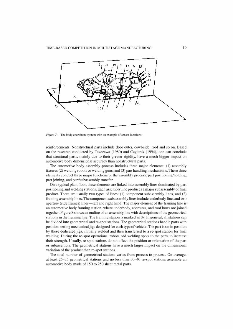
Figure 7. The body coordinate system with an example of sensor locations.

reinforcements. Nonstructural parts include door outer, cowl-side, roof and so on. Basedon the research conducted by Takezawa (1980) and Ceglarek (1994), one can concludethat structural parts, mainly due to their greater rigidity, have a much bigger impact onautomotive body dimensional accuracy than nonstructural parts.

The automotive body assembly process includes three major elements: (1) assemblyfixtures (2) welding robots or welding guns, and (3) part handling mechanisms. These threeelements conduct three major functions of the assembly process: part positioning/holding,part joining, and part/subassembly transfer.

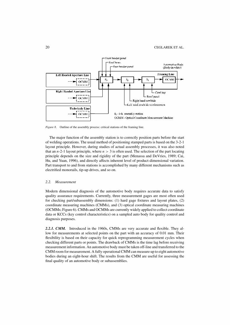
On a typical plant floor, these elements are linked into assembly lines dominated by partpositioning and welding stations. Each assembly line produces a major subassembly or finalproduct. There are usually two types of lines: (1) component subassembly lines, and (2)framing assembly lines. The component subassembly lines include underbody line, and twoaperture (side frames) lines—left and right hand. The major element of the framing line isan automotive body framing station, where underbody, apertures, and roof bows are joinedtogether. Figure 8 shows an outline of an assembly line with descriptions of the geometricalstations in the framing line. The framing station is marked as S3. In general, all stations canbe divided into geometrical and re-spot stations. The geometrical stations handle parts withposition-setting mechanical jigs designed for each type of vehicle. The part is set in positionby these dedicated jigs, initially welded and then transferred to a re-spot station for finalwelding. During the re-spot operations, robots add welding spots to the parts to increasetheir strength. Usually, re-spot stations do not affect the position or orientation of the partor subassembly. The geometrical stations have a much larger impact on the dimensionalvariation of the product than re-spot stations.

The total number of geometrical stations varies from process to process. On average,at least 25–35 geometrical stations and no less than 30–40 re-spot stations assemble anautomotive body made of 150 to 250 sheet metal parts.

20 CEGLAREK ET AL.

Figure 8. Outline of the assembly process: critical stations of the framing line.

The major function of the assembly station is to correctly position parts before the startof welding operations. The usual method of positioning stamped parts is based on the 3-2-1layout principle. However, during studies of actual assembly processes, it was also notedthat an n-2-1 layout principle, where n > 3 is often used. The selection of the part locatingprinciple depends on the size and rigidity of the part (Menassa and DeVries, 1989; Cai,Hu, and Yuan, 1996), and directly affects inherent level of product-dimensional variation.Part transport to and from stations is accomplished by many different mechanisms such aselectrified monorails, tip-up drives, and so on.

2.2. Measurement

Modern dimensional diagnosis of the automotive body requires accurate data to satisfyquality assurance requirements. Currently, three measurement gages are most often usedfor checking part/subassembly dimensions: (1) hard gage fixtures and layout plates, (2)coordinate measuring machines (CMMs), and (3) optical coordinate measuring machines(OCMMs; Figure 6). CMMs and OCMMs are currently widely applied to collect coordinatedata or KCCs (key control characteristics) on a sampled auto body for quality control anddiagnosis purposes.

2.2.1. CMM. Introduced in the 1960s, CMMs are very accurate and flexible. They al-low for measurements at selected points on the part with an accuracy of 0.01 mm. Theirflexibility is based on their capacity for quick reprogramming measurement cycles whenchecking different parts or points. The drawback of CMMs is the time lag before receivingmeasurement information. An automotive body must be taken off-line and transferred to theCMM room for measurement. A fully operational CMM can measure up to eight automotivebodies during an eight-hour shift. The results from the CMM are useful for assessing thefinal quality of an automotive body or subassemblies.


2.2.2. OCMM (Figure 6). In recent years, the implementation of the in-line optical co-ordinate measurement machine (OCMM) in automotive industry has provided new oppor-tunities for automotive body assembly diagnosis. OCMMs are installed in-line at the endof major assembly processes, such as framing, side frames, underbody, etc. (Figure 8).Each OCMM consists of several laser sensors allowing for noncontact measurement ofa body or subassembly relative to design nominal. On average, the measurement cycletakes a few seconds, with accuracy around 0.25 mm, and static and dynamic repeatabil-ity within 6-σ equal to 0.14 and 0.25 mm, respectively (Perceptron, 1991). The OCMMgage measures from 100 to 150 points on each major assembly with 100% sample rate.As a result, the OCMM provides a tremendous amount of dimensional information, whichcan be used for assembly process control. All OCMMs in the plant use the same coordi-nate system, called the body coordinate system, because it is easy to use and comparesdata from different gages. Figure 7 shows the coordinate axes and reference points in thebody coordinate system. The principles of the measurement sensors are described by Greer(1988), and the outline of the sensor setup for automotive body assembly can be found in Hu(1990).

2.3. Product development phases

A characteristic feature of the automotive industry is the frequency of model changes andthe vast amounts of time and labor required to make a changeover. The automotive bodyassembly is regarded as the least flexible process in the overall vehicle assembly (Sekine,Koyama, and Imazu, 1991). During a model change, tooling must be changed to matchthe newly established process and product design. Given the complexity of this process,the automotive body development cycle requires three to four years of lead time. Even thefinal stage of the automotive body development cycle, after vehicle and hard tooling aredesigned, lasts for about a year. This final stage includes the following phases: (1) pilotprogram, (2) prevolume production, (3) launch, and (4) full production. These phases aredescribed below, focusing on the dimensional issues.

The pilot program starts when prototype vehicles are built to verify manufacturing pro-cesses after 100% of the vehicle dimensions and tolerances are approved. The pilot programis the first phase, beginning on average five months ahead of the launch. It includes (a) verify-ing the designed KCC (key control characteristics; locators and clamps positions) schemesfor tooling fixtures during the assembly process; and (b) setting the process capability ofthe designed tooling.

Prevolume production starts 1–2 months ahead of launch, after the tooling is set up atthe assembly plant. The goal of prevolume production is to validate process capability andinitially identify the sources of variation.

After determining that the vehicle can reach acceptable quality levels, the launch phasefollows. Typically, at launch phase, a number of problems must still be resolved before avehicle of desired quality level can be built. The length of the launch phase depends on howquickly dimensional problems can be resolved while simultaneously speeding up productionrate. Identification of dimensional faults becomes one of the bottlenecks in reaching fullproduction rate.

22 CEGLAREK ET AL.

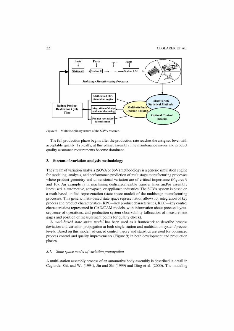
Figure 9. Multidisciplinary nature of the SOVA research.

The full production phase begins after the production rate reaches the assigned level withacceptable quality. Typically, at this phase, assembly line maintenance issues and productquality assurance requirements become dominant.

3. Stream-of-variation analysis methodology

The stream of variation analysis (SOVA or SoV) methodology is a generic simulation enginefor modeling, analysis, and performance prediction of multistage manufacturing processeswhere product geometry and dimensional variation are of critical importance (Figures 9and 10). An example is in machining dedicated/flexible transfer lines and/or assemblylines used in automotive, aerospace, or appliance industries. The SOVA system is based ona math-based unified representation (state-space model) of the multistage manufacturingprocesses. This generic math-based state space representation allows for integration of keyprocess and product characteristics (KPC—key product characteristics, KCC—key controlcharacteristics) represented in CAD/CAM models, with information about process layout,sequence of operations, and production system observability (allocation of measurementgages and position of measurement points for quality check).

A math-based state space model has been used as a framework to describe processdeviation and variation propagation at both single station and multistation system/processlevels. Based on this model, advanced control theory and statistics are used for optimizedprocess control and quality improvements (Figure 9) in both development and productionphases.

3.1. State space model of variation propagation

A multi-station assembly process of an automotive body assembly is described in detail inCeglarek, Shi, and Wu (1994), Jin and Shi (1999) and Ding et al. (2000). The modeling


Figure 10. Modeling of SOVA in manufacturing processes.

of fixture-related variation propagation in such an assembly process has been studied byMantripragada and Whitney (1999), Jin and Shi (1999), Lawless, Mackay, and Robinson(1999), Ding et al. (2000), and Camelio, Hu, and Ceglarek (2003). For purposes of illustra-tion, an example of state space modeling for automobile body assembly is presented belowwhich accounts for two major variation contributors. These two factors are fixture variationat each single station (Figure 11(a)), where δP2(z) is the deviation in Z -direction at locatorP2; and station-to-station correlation errors or the reorientation-induced variation when anassembly is transferred to another station (Figure 11(b)).

A multistage assembly system (Figure 12) is composed of a series of single stations.The variation propagation throughout the entire system can be modeled by using a state

Figure 11. Variation induced at a single station and across stations.

24 CEGLAREK ET AL.

Figure 12. Diagram of an assembly process with N stations.

space representation (Jin and Shi, 1999; Ding et al., 2000; Camelio et al., 2003). The statevector describes the geometrical errors of all relevant components in the system. Similar toa sequential dynamic system, this specific state space model uses a station index to replacethe time index in a traditional state space model. The state space transfer or the transmittedrelations between stations can thus be set up as the following two equations:

X(k) = A(k − 1)X(k − 1) + B(k)U(k) + W(k), (1)

Y(k) = C(k)X(k) + V(k), (2)

where X(k) is the state vector or product quality information (e.g., part dimensional devia-tions) after operations at station k. U(k) stands for the process variation contributed at stationk. Product measurements of key product characteristics (KPC) at station k are included inY(k), and W(k) and V(k) are unmodeled errors and sensor noise, respectively. Matrices A(k)and B(k) in the above model include information regarding process design such as fixturelayout on individual station k and the change of fixture layouts (datum transfer) across sta-tions, and C(k) includes sensor placement information (the number and location of sensorson station k). The corresponding physical interpretation of A, B, and C is presented inTable 1, where Φ(k, j) ≡ A(k − 1) · · · A( j) and Φ( j, j) ≡ I, and the detailed expression

Table 1. Interpretation of system matrices.

Symbol Name Relationship Interpretation Assembly task

A Dynamic matrix X(k − 1)A(k−1)−→ X(k) Change of fixture

layout between twoadjacent stations

Assembly transfer

Φ(k, i) State transition matrix X(i)Φ(k,i)−→ X(k) Change of fixture

layout amongmultiple stations

Assembly transfer

B Input matrix U(k)B(k)−→ X(k) Fixture layout at

station kPart positioning

C Observation matrix X(k)C(k)−→ Y(k) Sensor layout at

station kInspection


can be found in Ding et al. (2000). Suppose there is only end-of-line observation, that is,k = N in the observation equation of equation (2). Then, we have

Y(N ) =N∑

k=1

C(N )Φ(N , k)B(k)U(k) + C(N )Φ(N , 0)X(0) + ε. (3)

Here, X(0) corresponds to the initial condition, resulting from imperfectly manufacturedstamped parts, and ε is the summation of all modeling uncertainty and sensor noise terms.Moreover, it was assumed that this process involves sheet metal assembly with only lap-lapjoint and thus, the stamping imperfection of part dimensions will not affect the propagationof variations (Ceglarek and Shi, 1998). Then, we can set initial conditions to zero. Theuncertainty term ε can be neglected in the design stage.

The variation propagation can then be approximated as

KY =N∑

k=1

γ(k)KU (k)γT (k), (4)

where KY and KU (k) represent the covariance matrices of Y(N) and U(k), respectively, andγ(k) = C(N )Φ(N , k)B(k). Thus, product quality is affected by KU (k), the covariance ofprocess variables. Based on the engineering knowledge, it is known that process variablein this problem is related to fixturing error at every assembly station, which is often causedby the clearance of locating pinhole pairs.

4. Applications

4.1. Fixture fault diagnosis in manufacturing phase

This section will deal with the application of the state space model for fixture faults diagnosisin multistage manufacturing system (MMS). The propagation of deviation in an N -stationMMS can be represented in the form of state space equations (1) and (2), where k ⊂1, 2, . . . , N . Unmodeled noises V and W are assumed to be mutually independent. Thesedefinitions follow the same notation as used in Ding et al. (2000). Matrices A, B, and Cencode the design information of process configuration.

Equation (1) implies that part deviation at station i is influenced by two sources: theaccumulated part deviation up to station i − 1, and the deviation contributed at the currentstation. Equation (2) is the observation equation. If sensors are installed at one or morestations in a production line, the index for the observation equation is actually a subset of{1, 2, . . . , N }, whereas the index for the state equation is the complete set.

Assume that the end-of-line sensing strategy, the most commonly used sensor installationscheme in industrial setting, is employed. End-of-line sensing means that observation is onlyavailable at the last station N , that is, k = N for equation (2), and

Y = CX(N ) + V (5)

26 CEGLAREK ET AL.

where Y ∈ Rq×1 indicates that q measurements are obtained at station N . The indicesfor Y, C, and W are dropped since they are all Ns. The input–output relationship can berepresented as

Y =N∑

k=1

γ(k)U(k) + γ(0)X(0) + ε. (6)

Here, X(0), W, V are the basic random variables in a stochastic process and thus, usuallyassumed to be independent. The assumption can be partially released to include the situationwhere the basic random variables are dependent by enlarging the state vector. Moreover, U,the fixturing deviations at station k, are independent with those basic random variables aswell since only an open loop system is now being considered. Given the independent rela-tionships between these variables, the input–output covariance relationship can be obtainedfrom equation (6) to characterize the variation propagation in a production line,

KY =N∑

k=1

γ(k)KU (k)γT (k) + γ(0)K0γT (0) + Kε, (7)

where KY represents the covariance matrix of random vector Y, and K0 is given as theinitial variability condition. Kε can be estimated from the data when no fixture fault waspresent.

It is assumed that only the lap joints are involved in the current model, implying thatfabrication imperfection of parts will not affect the propagation of variations. Thus, it isreasonable to set the initial condition K0 to zero. The process can then be approximated asfollows:

KY =N∑

k=1

γ(k)KU (k)γT (k) + Kε. (8)

This equation suggests that while being contaminated by noise, the variation of the finalproduct is mainly the contribution of variations of fixturing errors at all stations.

Without considering the matrix Kε, we have

K0Y =

N∑k=1

γ(k)KU (k)γT (k).

It has been proven by Ceglarek and Shi (1996) and Ding et al. (2002b) that the eigenvalue–eigenvector pair {λkp,γ p(k)} of matrix K0

Y can be used for fixture fault diagnosis, λkp

represents the variance of the principal component at station k caused by fault p. Theeigenvector is the pattern vector of this fixture fault, manifesting the fixturing variation bygenerating a mode shape of measurement vector Y. In the rest of this paper, assume γ p(k)as a normalized eigenvector using the Euclidean norm.

The basic concept of the diagnostic methodology is shown in Figure 13. If a fault offixture element (locator) exists in a station, a symptom will be reflected in the final product


Figure 13. Outline of the diagnostic methodology.

or downstream intermediate products. From off-line CAD information and the state spacemodel, a set of all possible fault patterns can be generated. Measurement data are col-lected in-line (OCMM) and analyzed using one of the multivariate statistical methods,for example, the principal component analysis (PCA), to extract the fault feature patterns.Fault isolation can then be conducted by mapping the feature patterns of real produc-tion data with predetermined fault patterns generated from the analytical model. Thiscan be done by calculating the similarity of the two patterns. The similarity of any twopattern vectors γ p(i) and γq (k) is defined as the acute angle formed by fault patternvectors

θpq (i, k) = cos−1〈γ p(i),γq (k)〉, 0 ≤ θ ≤ π

2,

where 〈·, ·〉 represents the inner product of two vectors. The least acute angle betweenmeasured pattern vector and one of the potential fault pattern vector reveals the mostlikely fault and its location. It is obvious that if the least angle between any pair of pos-sible fault patterns is too small then they may not be easily distinguishable under thecontamination of possible noises, so that the similarity analysis has to be done beforediagnosis.

4.1.1. Case study. A multistage process is set up, which is abstracted from a side aper-ture assembly line in the automotive industry, including three assembly stations and onemeasurement station. The final product is made of four parts, as shown in Figure 14.

The assembly sequence and datum shift scheme regarding this assembly process areshown in Figure 15. {{P1, P2}, {P3, P4}} denotes the locating pairs used at station 1, with{P1, P2} and {P3, P4} depicting the first and the second parts, respectively. The others are

28 CEGLAREK ET AL.

Figure 14. Geometry of the assembly.

Figure 15. Assembly sequence and datum shift scheme.

similarly defined. At station 4, which is the measurement station, one pair of locating pins{P1, P8} is used since there is only one piece of the assembly to measure.

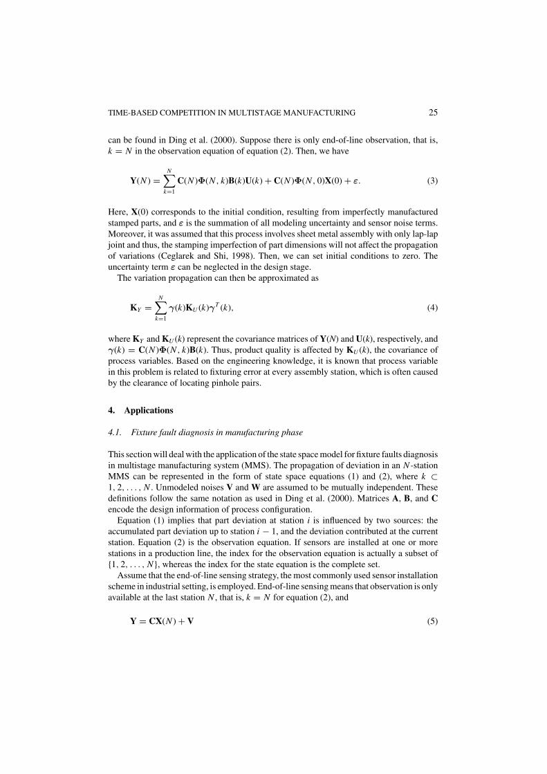
As shown in Figure 14(b), part motion in both X and Z directions are controlled by4-way pins of P1, P3, P5, and P7 and in the Z direction by 2-way pins of P2, P4, P6, and P8.It is also assumed that the fixture error at the measurement station can be neglected whencompared with assembly fixtures. The relationship between fault indices and root causeson each station is shown in Table 2 and in Figure 16.

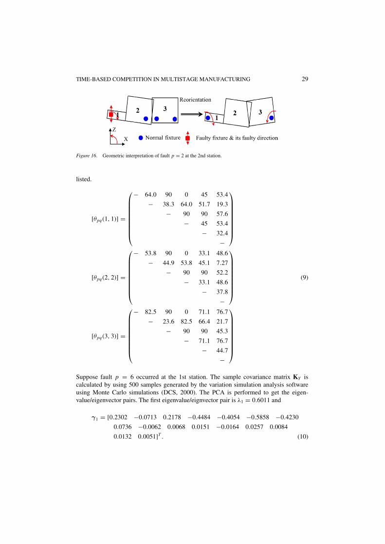
As indicated in Figure 14(b), there are two sensors on each part at the last station (end-of-line sensing). Each sensor can measure part deviation in both X and Z directions. Twosensors are sufficient to detect the deviation in position and orientation of a 2D rigid part.The angles (in degree) between all fault pattern vectors at station i are listed as follows,where p, q = 1, 2, 3, 4, 5, 6. Since these matrices are symmetric, only the upper half is

Table 2. Fault indices and their root causes.

Index Fault root cause Index Fault root cause

p = 1 4-way pin on the 1st part/subassembly isfaulty in X -direction

p = 4 4-way pin on the 2nd part/subassembly isfaulty in X -direction

p = 2 4-way pin on the 1st part/subassembly isfaulty in Z -direction

p = 5 4-way pin on the 2nd part/subassembly isfaulty in Z -direction

p = 3 2-way pin on the 1st part/subassembly isfaulty in Z -direction

p = 6 2-way pin on the 2nd part/subassembly isfaulty in Z -direction


Figure 16. Geometric interpretation of fault p = 2 at the 2nd station.

listed.

[θpq (1, 1)] =

− 64.0 90 0 45 53.4

− 38.3 64.0 51.7 19.3

− 90 90 57.6

− 45 53.4

− 32.4

−

[θpq (2, 2)] =

− 53.8 90 0 33.1 48.6

− 44.9 53.8 45.1 7.27

− 90 90 52.2

− 33.1 48.6

− 37.8

−

(9)

[θpq (3, 3)] =

− 82.5 90 0 71.1 76.7

− 23.6 82.5 66.4 21.7

− 90 90 45.3

− 71.1 76.7

− 44.7

−

Suppose fault p = 6 occurred at the 1st station. The sample covariance matrix KY iscalculated by using 500 samples generated by the variation simulation analysis softwareusing Monte Carlo simulations (DCS, 2000). The PCA is performed to get the eigen-value/eigenvector pairs. The first eigenvalue/eignvector pair is λ1 = 0.6011 and

γ1 = [0.2302 −0.0713 0.2178 −0.4484 −0.4054 −0.5858 −0.4230

0.0736 −0.0062 0.0068 0.0151 −0.0164 0.0257 0.0084

0.0132 0.0051]T . (10)

30 CEGLAREK ET AL.

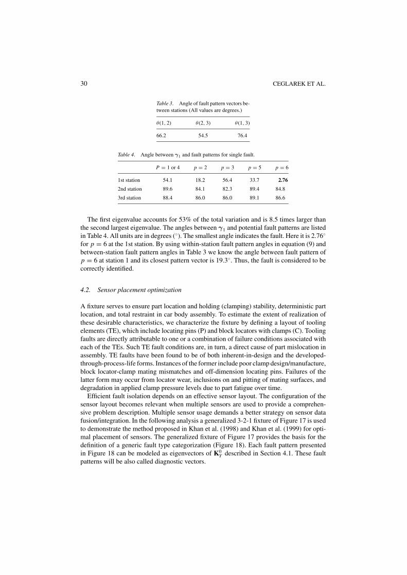
Table 3. Angle of fault pattern vectors be-tween stations (All values are degrees.)

θ (1, 2) θ (2, 3) θ (1, 3)

66.2 54.5 76.4

Table 4. Angle between γ1 and fault patterns for single fault.

P = 1 or 4 p = 2 p = 3 p = 5 p = 6

1st station 54.1 18.2 56.4 33.7 2.76

2nd station 89.6 84.1 82.3 89.4 84.8

3rd station 88.4 86.0 86.0 89.1 86.6

The first eigenvalue accounts for 53% of the total variation and is 8.5 times larger thanthe second largest eigenvalue. The angles between γ1 and potential fault patterns are listedin Table 4. All units are in degrees (◦). The smallest angle indicates the fault. Here it is 2.76◦

for p = 6 at the 1st station. By using within-station fault pattern angles in equation (9) andbetween-station fault pattern angles in Table 3 we know the angle between fault pattern ofp = 6 at station 1 and its closest pattern vector is 19.3◦. Thus, the fault is considered to becorrectly identified.

4.2. Sensor placement optimization

A fixture serves to ensure part location and holding (clamping) stability, deterministic partlocation, and total restraint in car body assembly. To estimate the extent of realization ofthese desirable characteristics, we characterize the fixture by defining a layout of toolingelements (TE), which include locating pins (P) and block locators with clamps (C). Toolingfaults are directly attributable to one or a combination of failure conditions associated witheach of the TEs. Such TE fault conditions are, in turn, a direct cause of part mislocation inassembly. TE faults have been found to be of both inherent-in-design and the developed-through-process-life forms. Instances of the former include poor clamp design/manufacture,block locator-clamp mating mismatches and off-dimension locating pins. Failures of thelatter form may occur from locator wear, inclusions on and pitting of mating surfaces, anddegradation in applied clamp pressure levels due to part fatigue over time.

Efficient fault isolation depends on an effective sensor layout. The configuration of thesensor layout becomes relevant when multiple sensors are used to provide a comprehen-sive problem description. Multiple sensor usage demands a better strategy on sensor datafusion/integration. In the following analysis a generalized 3-2-1 fixture of Figure 17 is usedto demonstrate the method proposed in Khan et al. (1998) and Khan et al. (1999) for opti-mal placement of sensors. The generalized fixture of Figure 17 provides the basis for thedefinition of a generic fault type categorization (Figure 18). Each fault pattern presentedin Figure 18 can be modeled as eigenvectors of K0

Y described in Section 4.1. These faultpatterns will be also called diagnostic vectors.


Figure 17. 3-2-1 Fixture layout.

Figure 18. 3-2-1 Fault manifestations (Khan et al., 1999).

32 CEGLAREK ET AL.

An optimal sensor location can be obtained by maximizing the minimum distance betweeneach pair of dominant eigenvectors of K0

Y , and obtained for each of the tooling faults. Theconnotation of the maximization premise is to increase the power, or the degree of reliability,of the discriminant. Here the discriminant serves in a pattern recognition sense, as anestimator of the membership of each observed or hypothesized fault to one of the fault typeclass. Efficient fault discrimination (diagnosis) is thus possible if the sensor locale providesa maximal spread of fault type classes in space. In the event of sensor noise or multiple faulttype coexistence, the primary fault type associated with the prominent eigenvector can bereadily distinguished.

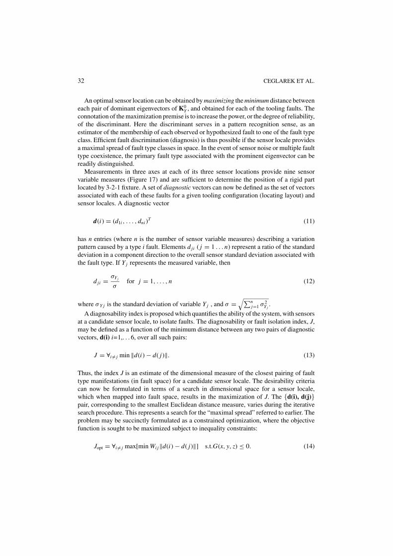
Measurements in three axes at each of its three sensor locations provide nine sensorvariable measures (Figure 17) and are sufficient to determine the position of a rigid partlocated by 3-2-1 fixture. A set of diagnostic vectors can now be defined as the set of vectorsassociated with each of these faults for a given tooling configuration (locating layout) andsensor locales. A diagnostic vector

d(i) = (d1i , . . . , dni )T (11)

has n entries (where n is the number of sensor variable measures) describing a variationpattern caused by a type i fault. Elements d ji ( j = 1 . . . n) represent a ratio of the standarddeviation in a component direction to the overall sensor standard deviation associated withthe fault type. If Y j represents the measured variable, then

d ji = σY j

σfor j = 1, . . . , n (12)

where σ Y j is the standard deviation of variable Y j , and σ =√∑n

j=1 σ 2Y j

.

A diagnosability index is proposed which quantifies the ability of the system, with sensorsat a candidate sensor locale, to isolate faults. The diagnosability or fault isolation index, J,may be defined as a function of the minimum distance between any two pairs of diagnosticvectors, d(i) i=1,. . . 6, over all such pairs:

J = ∀i �= j min ‖d(i) − d( j)‖. (13)

Thus, the index J is an estimate of the dimensional measure of the closest pairing of faulttype manifestations (in fault space) for a candidate sensor locale. The desirability criteriacan now be formulated in terms of a search in dimensional space for a sensor locale,which when mapped into fault space, results in the maximization of J. The {d(i), d(j)}pair, corresponding to the smallest Euclidean distance measure, varies during the iterativesearch procedure. This represents a search for the “maximal spread” referred to earlier. Theproblem may be succinctly formulated as a constrained optimization, where the objectivefunction is sought to be maximized subject to inequality constraints:

Jopt = ∀i �= j max[min Wi j‖d(i) − d( j)‖] s.t.G(x, y, z) ≤ 0. (14)


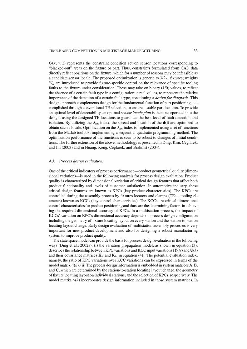
G(x, y, z) represents the constraint condition set on sensor locations corresponding to“blacked-out” areas on the fixture or part. Thus, constraints formulated from CAD datadirectly reflect positions on the fixture, which for a number of reasons may be infeasible asa candidate sensor locale. The proposed optimization is generic to 3-2-1 fixtures; weightsWij are introduced to provide fixture-specific control on the relevance of specific toolingfaults to the fixture under consideration. These may take on binary (1/0) values, to reflectthe absence of a certain fault type in a configuration; r real values, to represent the relativeimportance of the detection of a certain fault type, constituting a design for diagnosis. Thisdesign approach complements design for the fundamental function of part positioning, ac-complished through conventional TE selection, to ensure a stable part location. To providean optimal level of detectability, an optimal sensor locale plan is then incorporated into thedesign, using the designed TE locations to guarantee the best level of fault detection andisolation. By utilizing the Jopt index, the spread and location of the d(i) are optimized toobtain such a locale. Optimization on the Jopt index is implemented using a set of functionsfrom the Matlab toolbox, implementing a sequential quadratic programming method. Theoptimization performance of the functions is seen to be robust to changes of initial condi-tions. The further extension of the above methodology is presented in Ding, Kim, Ceglarek,and Jin (2003) and in Huang, Kong, Ceglarek, and Brahmst (2004).

4.3. Process design evaluation.

One of the critical indicators of process performance—product geometrical quality (dimen-sional variation)—is used in the following analysis for process design evaluation. Productquality is characterized by dimensional variation of critical design features that affect bothproduct functionality and levels of customer satisfaction. In automotive industry, thesecritical design features are known as KPCs (key product characteristics). The KPCs arecontrolled during the assembly process by fixtures locators and clamps (TEs—tooling el-ements) known as KCCs (key control characteristics). The KCCs are critical dimensionalcontrol characteristics for product positioning and thus, are the determining factors in achiev-ing the required dimensional accuracy of KPCs. In a multistation process, the impact ofKCCs’ variation on KPC’s dimensional accuracy depends on process design configurationincluding the geometry of fixture locating layout on every station and the station-to-stationlocating layout change. Early design evaluation of multistation assembly processes is veryimportant for new product development and also for designing a robust manufacturingsystem to improve product quality.

The state space model can provide the basis for process design evaluation in the followingways (Ding et al., 2002a): (i) the variation propagation model, as shown in equation (3),describes the relationship between KPC variations and KCC input variations (Y(N) and U(k)and their covariance matrices KY and KU in equation (4)). The potential evaluation index,namely, the ratio of KPC variations over KCC variations can be expressed in terms of themodel matrixγ(k). (ii) The process design information is embedded in system matrices A, B,and C, which are determined by the station-to-station locating layout change, the geometryof fixture locating layout on individual stations, and the selection of KPCs, respectively. Themodel matrix γ(k) incorporates design information included in those system matrices. In

34 CEGLAREK ET AL.

short, the aforementioned two items (i) and (ii) imply that the state space model integratesrich process design information, serving as the basis for the development of desirabledesign evaluation indices. The evaluation of multistation assembly process design can thenbe conducted parallel to the sensitivity analysis of a dynamic system.

A single design evaluation index is inadequate to describe critical aspects of varia-tion propagation in a multistation assembly system. The index based on the entire systemvariation input and output characterizes the overall process performance, however, it doesnot provide any detailed information about an individual station or a single fixture. On theother hand, the index based on the variation input and output of a single fixture character-izes the performance of a single fixture during production, but it does not provide the jointeffect of multiple variation inputs at the system level. Therefore, a group of hierarchicalmultilevel indices is developed to capture critical aspects of the variation behavior of amultistation assembly process. Furthermore, these multilevel indices are expressed in termsof critical process design characteristics and are independent of variation inputs since it isthe design configuration that needs to be evaluated rather than the transmitted variation asit was presented in section 4.1.

For the N-station assembly process shown in Figure 12, the KPC variation is denotedas a variance vector, σ2

output, with elements that are the diagonal elements of KY , i.e.,σ2

output = diag(KY ). The KCC variation inputs are decomposed into three levels. Variationσ 2

kp at the single fixture level stands for the variance of the pth locating feature at station k.Variation vector σ2

k at a single station level is denoted as

σ2k = [

σ 2k1 · · · σ 2

kp · · · σ 2kmk

]T.

It is easy to verify that σ2k = diag(Kp(k)). Variation vector σ2

input represents the variationinputs of the entire process and is defined as

σ2input = [

σ2T

1 · · ·σ2T

k · · · σ 2T

N

]T.

The sensitivity analysis for design evaluation defines: (1) how the system responds tocertain variation inputs; (2) which variation source contributes most to the final productvariation; and/or (3) how related process parameters account most for the variation prop-agation. As such, the sensitivity indices are similar to the system gains in control theory.Appropriate measure is introduced to represent process sensitivity as the gain of a multiple-input-multiple-output (MIMO) system. Three-level sensitivity indices are defined to facili-tate the description of the system behavior of a multistation assembly process: single fixturelevel, station level with multiple fixtures, and system level (multistation).

The design evaluation index (DEI) at the fixture level, denoted as Skp, is defined as

Skp =∥∥Wσ 2

output

∥∥2

σ 2kp

. (15)


where weighting coefficient W determines the relative importance of KPC variances and‖ · ‖2 is the Euclidean norm. Skp index indicates how the pth locating feature at station kcontributes to the KPC variations. In fact, at this level, Skp, corresponds to the gain of aSingle-Input-Multiple-Output (SIMO) system.

The DEI at the station level, denoted as Sk , is defined as

Sk = supσ2k

∥∥Wσ2output

∥∥2∥∥σ2

k

∥∥2

. (16)

Sk index indicates how the fixture elements on station k jointly affect the KPC variation. Itis a MIMO-type gain since each station contains multiple fixtures. Station-level sensitivityindex Sk identifies the critical station contributing most to the KPC variation.

The DEI at the system level, denoted as So, is defined as

So = supσ2

input

∥∥Wσ2output

∥∥2∥∥σ2

input

∥∥2

(17)

So index indicates the system capacity to amplify or suppress the input variations. So indexis also a MIMO-type gain.

The aforementioned defined indices Skp, Sk , and So are the ratios of KPC variation overthe KCC variation. Consider ‖Wσ 2

output‖2 as the indicator of KPC variation level. IndicesSkp, Sk , and So are the values of KPC variation given a unit KCC variation input. The unitof KCC variation is different for the three indices: for a single fixture, a unit KCC variationis equivalent to σ 2

kp = 1; for a station, a unit KCC variation is the joint effect from themultiple fixtures, defined as ‖σ2

k‖2 = 1; for the entire system, a unit KCC variation is thecombined effect from the multiple stations, defined as ‖σ2

input‖2 = 1. A sensitivity indexless than 1 means that the KPC variation level can become lower than the KCC variationlevel. On the contrary, a sensitivity index larger than 1 implies that the system amplifiesthe input variation. Most of the multistation systems will end up with a sensitivity greaterthan 1. Nonetheless, a smaller sensitivity value suggests a less variation-sensitive systemwhich is preferable. Therefore, using and comparing this group of indices, a robust processconfiguration can be selected and the sensitive station and fixture can be identified andprioritized.

Next, the indices Skp, Sk , and So are expressed in terms of the model matrix γ so thatthey are made input independent.

It has been proved that if the KCC variation inputs in Figure 11 are uncorrelated, theKPC variance vector σ2

output can be represented as a linear combination of the vector σ2k .

The expression can be represented as

σ2output =

N∑k=1

[γ2(k)] · σ2k (18)

36 CEGLAREK ET AL.

where [γ2(k)] represents a matrix in which each element is the square of the correspondingelement in matrix γ(k), i.e.,

[γ2] =

γ 211 γ 2

12 · · · γ 21m

γ 221 γ 2

22 · · · γ 22m

......

. . ....

γ 2q1 γ 2

q2 · · · γ 2qm

. (19)

According to the definition of Skp index, it is assumed that there is only a single variationsource (rather than multiple simultaneous sources) in the entire process at each time.

The fixture-level sensitivity index Skp for the pth KCC on station k can be proved (Dinget al., 2002a) to be

Skp = ∥∥W · γ2p(k)

∥∥2 (20)

The second index is the station sensitivity index Sk . It is assumed that only one station hasvariation inputs at a time. But within each station, more than one fixture element couldcontribute to σ2

output simultaneously.The station-level sensitivity index Sk can be expressed as Ding et al. (2002a)

Sk = ‖W · [γ2(k)]‖2. (21)

System-level sensitivity will consider all possible combinations of multiple KCC variationinputs—within a station and/or cross-stations. Thus, it represents the overall sensitivitylevel of a process as to the KCC variation inputs.

The system-level sensitivity index So can be expressed as Ding et al. (2002a)

So = ‖W · [γ2(1)γ2(2) · · ·γ2(N )]‖2. (22)

It is also possible to define the station and system sensitivity indices using the fixturesensitivity index, that is, choosing the largest fixture sensitivity index within a station or ina process as the station and system indices, respectively. Under this definition, these newindices could represent process response to a single variation input, whereas the proposedindices (equations (16) and (17)) describe the joint effect of multiple simultaneous variationinputs. The results are different using the two sets of definitions. The selection between bothsets of indices depends on the specific requirements of applications.

Case study. The assembly process of the sport utility vehicle (SUV) side panel is usedto illustrate the concepts of sensitivity analysis and demonstrate the design evaluationmethodology. In addition to KCCs P1–P8 used in the assembly process, there is an extralocating hole P9 (Figure 19) on the rear quarter panel which can be used to first position


Figure 19. KCCs P1–P9 on the assembly.

this panel on station III, and then the whole subassembly on the measurement station.The nominal design positions of the fixture locators (KCCs) and KPC points in 2D (X–Zcoordinates) are given in Tables 5 and 6, respectively.

Four alternative process configuration schemes marked as C1–C4 are used for evaluation.Configuration C1 is currently used in one US automotive assembly plant and is utilized hereas the reference in our design evaluation. A major difference between other configurations(C2, C3, C4) and C1 is that locator P9 is used to replace P7 when the rear quarter panelis located on station III. The fixture locating layout for each configuration is presented inTable 7.

In order to evaluate the different design configurations, a state space model is developedfor the above four configurations, following methods presented in Jin and Shi (1999) andDing, et al. (2000). The sensitivity-based design evaluation is then conducted following the

Table 5. Coordinates of fixture locators (KCCs) from Figure 19 (units: mm).

KCC P1 P2 P3 P4 P5

(X, Z ) (367.8,906.05) (667.47,1295.35) (1301,1368.89) (1272.73,537.37) (1470.71,1640.40)

KCC P6 P7 P8 P9

(X, Z ) (1770.50,1702.62) (2941.42,1691.31) (2120.32,1402.83) (3026.25, 950.30)

Table 6. Coordinates of KPCs from Figure 20(d) (units: mm).

KPC M1 M2 M3 M4 M5

(X, Z ) (271.50,905) (565.7, 1634.7) (1289.7,1227.5) (1306.5,633.5) (1244.5,85)

KPC M6 M7 M8 M9 M10

(X, Z ) (1604.5,1781.8) (2884.8,1951.5) (2743.5,475.2) (1838.4,226.3) (1979.8,1459.4)

38 CEGLAREK ET AL.

Table 7. Process configuration schemes.

Configuration Assembly Sequence

C1 {{P1, P2}, {P3, P4}}I →{{P1, P4}, {P5, P6}}II →{{P1, P6}, {P7, P8}}III →{{P1, P8}}IV




three steps. During this case study, the weight coefficient matrix W is selected as an identitymatrix, implying that all KPCs are treated with equal importance.

Step 0: State space modeling of the assembly process. In this SUV side panel assemblyprocess, there are three assembly stations and one inspection station, i.e., N = 4 (seeFigure 20). The fixture used on the inspection station is considered well maintained andcalibrated with much higher repeatability than those on a regular assembly station. Thus,the input variation of fixture locators on the measurement station is neglected and the KCC

Figure 20. Assembly process of the side aperture panel of a SUV.


Table 8. Process sensitivity index for C1–C4 process configuration.

C1 C2 C3 C4

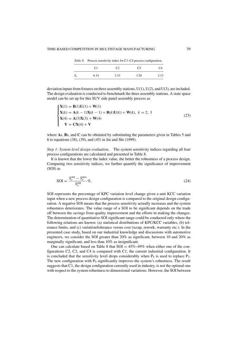
So 6.14 3.33 3.26 3.13

deviation inputs from fixtures on three assembly stations, U(1), U(2), and U(3), are included.The design evaluation is conducted to benchmark the three assembly stations. A state spacemodel can be set up for this SUV side panel assembly process as

X(1) = B(1)U(1) + W(1)

X(k) = A(k − 1)X(k − 1) + B(k)U(k) + W(k), k = 2, 3

X(4) = A(3)X(3) + W(4)

Y = CX(4) + V

(23)

where As, Bs, and C can be obtained by substituting the parameters given in Tables 5 and6 to equations (38), (39), and (45) in Jin and Shi (1999).

Step 1: System level design evaluation. The system sensitivity indices regarding all fourprocess configurations are calculated and presented in Table 8.

It is known that the lower the index value, the better the robustness of a process design.Comparing two sensitivity indices, we further quantify the significance of improvement(SOI) as

SOI = Soldo − Snew

o

Soldo

%. (24)

SOI represents the percentage of KPC variation level change given a unit KCC variationinput when a new process design configuration is compared to the original design configu-ration. A negative SOI means that the process sensitivity actually increases and the systemrobustness deteriorates. The value range of a SOI to be significant depends on the tradeoff between the savings from quality improvement and the efforts in making the changes.The determination of quantitative SOI significant range could be conducted only where thefollowing relations are known: (a) statistical distributions of KPC/KCC variables, (b) tol-erance limits, and (c) variation/tolerance versus cost (scrap, rework, warranty etc.). In thepresented case study, based on our industrial knowledge and discussions with automotiveengineers, we consider the SOI greater than 20% as significant, between 10 and 20% asmarginally significant, and less than 10% as insignificant.

One can calculate based on Table 8 that SOI = 45%–49% when either one of the con-figurations C2, C3, and C4 is compared with C1, the current industrial configuration. Itis concluded that the sensitivity level drops considerably when P9 is used to replace P7.The new configuration with P9 significantly improves the system’s robustness. The resultsuggests that C1, the design configuration currently used in industry, is not the optimal onewith respect to the system robustness to dimensional variations. However, the SOI between

40 CEGLAREK ET AL.

Table 9. Station sensitivity index for configuration C4.

Station I Station II Station III

Sk 2.94 1.69 3.01

any two of the other three process designs using P9 (options C2, C3, and C4) is smallerthan 6%. Therefore, their differences are not significant. The fourth scheme (C4) yieldsthe lowest So value among the four process configurations. The value of SOI equals 49.0%when C4 is compared with C1, which corresponds to a 49.0% decrease in KPC variationlevel under the same condition of KCC variation input. Hence, it is recommended that thecurrent process design should be replaced by configuration C4.

Step 2: Station level design evaluation. Let us further study the station sensitivity ofthe C4 configuration to identify which station has the largest contribution towards theKPC variation. Sensitivity indices for three stations are shown in Table 9. The percentageof variation contribution (PVC) from station k can be calculated using the followingindex

PVCk = Sk

�Nk=1Sk

%. (25)

One can find that PVC3 = 39.4%, PVC1 = 38.5%, and PVC2 = 22.1%. The thirdand most critical station produces the highest sensitivity and PVC value. Station I also hasremarkable contribution to the KPC variation. Stations I and III together account for 77.9%contribution in the KPC variation level. Station II has the lowest station sensitivity and thesmallest PVC value. It would be the designer’s highest priority to investigate the designlayouts of stations I and III.

Step 3: Fixture level design evaluation. Finally, the fixture sensitivity index is computed forevaluation. At each station, four independent locating pins position two parts/subassemblies.The total 12 indices are shown in Table 10.

From the above table, it can be ascertained that not all locators at station II are majorvariation contributors. Stations I and III include certain critical variation sources. Locators

Table 10. Fixture sensitivity index for configuration C4.

Station I Station II Station III

Locator 1 2.38 1.50 2.03

Locator 2 1.37 0.69 0.75

Locator 3 2.18 0.65 2.68

Locator 4 0.75 0.56 1.09


Figure 21. Comparison of sensitivity index from DCS and analytical approach.

1 and 3 (4-way locators) at stations I and III cause the largest variations in the final assemblyif the input variations have the same magnitude. The variation reduction and design effortshould be first focused on stations I and III to reduce the sensitivity of these two 4-waylocators.

A numeric variation simulation analysis software based on the Monte Carlo (DCS, 2000)can be used to obtain the sensitivity indices. As discussed earlier in this section, it is difficultand time consuming to compute MIMO-type of indices such as Sk and So using DCS. Thus,the DCS software is only used to obtain the fixture level sensitivity index Skp. An identicalassembly process as presented in the case study is modeled using the VSL language andthe numerical variation model is generated in the DCS. A normal variation source with3σ = 1 is assigned to one fixture locator each time, and 5000-run Monte Carlo simulationsare then conducted. The sensitivity index is computed by dividing the KPC variation bythe input source’s variance. The results are compared with those values in Table 10, whichare calculated from design parameters using analytical formulations. The comparison isshown in Figure 21, where we can observe good consistency between the analytical andnumerical calculations of fixture level sensitivity index. The maximum difference is lessthan 3.2%.

5. Conclusions

Currently, a new paradigm is emerging in manufacturing and design in which increasedcustomization, product proliferation, heterogeneous markets, shorter product life cycle anddevelopment time, responsiveness etc. are increasingly taking center stage. One of the char-acteristic features of the modern manufacturing and new product development in automotive,aerospace, and other industries is the frequency of model change and the vast amounts oftime and cost required to make a changeover, also called time-based competition. This trendhas continuously gone up in the last two decades.

42 CEGLAREK ET AL.

A major obstacle in effective time-based competition is the often costly, difficult and time-consuming identification of root causes of the stream of variation (dimensional variationpropagation) in complex multistage manufacturing systems.

This paper discusses the concept of time-based competition in manufacturing and designbased on the review of on-going research related to stream-of-variation (SOVA) methodol-ogy. The presented methodology is based on the state space model characterizing variationpropagation in a multistage process. The state space model describes a discrete-time LTV(linear time varying) stochastic system, which strongly indicates that the existing systemand control theory could be used to perform systematic analysis and achieve variation con-trol of the manufacturing process. Moreover, the state space model integrates informationof product quality with process information such as tooling status, therefore, providingthe basis for fault diagnosis. The model is validated through simulation comparison withthe widely used variation simulation software 3DCS (DCS, 2000). The applications of thepresented SOVA model for dimensional fault diagnostics, design evaluation, and sensorplacement are presented.

While the presented research is conducted within the context of automotive assemblyprocess, the methodology is applicable to generic multistage manufacturing processes.

Acknowledgments

The authors gratefully acknowledge the financial support of the National Science Founda-tion award DMI-0239244 and the NIST Advanced Technology Program (ATP CooperativeAgreement # 70NANB3H3054).

References

Apley, D. W. and Shi, J., “Diagnosis of Multiple Fixture Faults in Panel Assembly,” ASME Journal of ManufacturingScience and Engineering, Vol. 120, pp. 793–801 (1998).

Baron, J., “Dimensional Analysis and Process Control of Body-In-White Processes,” Ph. D. Dissertation, Universityof Michigan, Ann Arbor, MI (1992).

Bollinger, J. E. (Ed.), Visionary Manufacturing Challenges for 2020, Committee on Visionary ManufacturingChallenges, National Research Council, National Academy Press, Washington, DC (1998).

Cai, W., Hu, S. J., and Yuan J. X., “Deformable Sheet Metal Fixturing: Principles, Algorithms, and Simulations,”Transactions of ASME, Journal of Manufacturing Science and Engineering, Vol. 118, No. 3, pp. 318–324(1996).

Camelio, J., Hu, S. J., and Ceglarek, D., “Modeling Variation Propagation of Multi-Station Assembly Systemswith Compliant Parts,” Transactions of ASME, Journal of Mechanical Design, Vol. 125, No. 4, pp. 673–681(2003).

Ceglarek, D., “Knowledge-Based Diagnosis for Automotive Body Assembly: Methodology and Implementation,”Ph.D. Dissertation, University of Michigan, Ann Arbor, MI (1994).

Ceglarek, D. and Shi, J., “Dimensional Variation Reduction for Automotive Body Assembly Manufacturing,”Manufacturing Review, Vol. 8, No. 2, pp. 139–154 (1995).

Ceglarek, D. and Shi, J., “Fixture Failure Diagnosis for Auto Body Assembly Using Patter Recognition,” ASMETransactions, Journal of Engineering for Industry, Vol. 118, No. 1, pp. 55–65 (1996).

Ceglarek, D. and Shi, J., “Design Evaluation of Sheet Metal Joints for Dimensional Integrity,” Transactions ofASME, Journal of Manufacturing Science and Engineering, Vol. 120, No. 2, pp. 452–460 (1998).


Ceglarek, D., Shi, J., and Wu, S. M., “A Knowledge-Based Diagnosis Approach for the Launch of the Auto-BodyAssembly Process,” Transactions of ASME, Journal of Engineering for Industry, Vol. 116, No. 4, pp. 491–499(1994).

Chase, K. W. and Parkinson, A. R., “A Survey of Research in the Application of Tolerance Analysis to the Designof Mechanical Assemblies,” Res. Eng. Design, Vol. 3, pp. 23–37 (1991).

CIRP, “Flexible Automation—Assessment and Future,” CIRP Scientific Technical Committee Survey in USA,Europe and Japan (January 27, 2000).

DCS, 3D Variation Simulation, Dimensional Control Systems, Inc. (2000).Ding, Y., Ceglarek, D., and Shi, J., “Modeling and Diagnosis of Multistage Manufacturing Process: Part I State

Space Model,” Proceedings of 2000 Japan–USA Symposium on Flexible Automation, July 23–26, Ann Arbor,MI, 2000JUSFA-13146 (2000).

Ding, Y., Ceglarek, D., and Shi, J., “Design Evaluation of Multi-station Assembly Processes by Using State SpaceApproach,” ASME Transactions, Journal of Mechanical Design, Vol. 124, No. 3, pp. 408–418 (2002a).

Ding, Y., Ceglarek, D., and Shi, J., “Fault Diagnosis of Multistage Manufacturing Processes by Using StateSpace Approach,” ASME Transactions, Journal of Manufacturing Science and Engineering, Vol. 124, No. 2,pp. 313–322 (2002b).

Ding, Y., Shi, J., and Ceglarek, D., “Diagnosability Analysis of Multistage Manufacturing Processes,” ASMETransactions, Journal of Dynamic Systems, Measurement, and Control, Vol. 124, No. 1, pp. 1–13 (2002c).

Ding, Y., Kim, P., Ceglarek, D., and Jin, J., “Optimal Sensor Distribution for Variation Diagnosis in Multi-StationManufacturing Processes,” IEEE Transactions on Robotics and Automation, Vol. 19, No. 4, pp. 543–556 (2003).

El-Gizawy, A. S., Hwang, J.-Y., and Brewer, D. H., “A Strategy for Integrating Product and Process Design ofAerospace Components,” Manufacturing Review, Vol. 3, No. 3, pp. 178–186 (1990).

ERC-RMS, National Science Foundation–Engineering Research Center for Reconfigurable Manufacturing Sys-tems (ERC-RMS), Technical Report, University of Michigan (1999).

Gadh, R., “A Hybrid Approach to Intelligent Geometric Design Using Features-Based Design and Feature Recog-nition,” Proceedings of the 19th Annual ASME Design Automation Conference, Vol. DE-65, No. 2, pp. 273–283(1993).

Gerwin, D. and Barrowman, N. J., “An Evaluation of Research on Integrated Product Development,” ManagementScience, Vol. 48, No. 7, pp. 938–953 (2002).

Greer, D., “On-line Machine Vision Sensor Measurements in a Coordinate System,” SME Paper #IQ88–289(1988).

Hu, S. J., “Impact of 100% Measurement Data on Statistical Process Control (SPC) in Automobile Body Assembly,”Ph.D. Dissertation, University of Michigan, Ann Arbor, MI (1990).

Hu, S. J., “Stream-of-Variation Theory for Automotive Body Assemblies,” Annals of CIRP, Vol. 46, No. 1, pp. 1–6(1997).

Hu, S. and Wu, S. M., “Identifying Root Causes of Variation in Automobile Body Assembly Using PrincipalComponent Analysis,” Transactions of NAMRI, Vol. 20, pp. 311–316 (1992).

Huang, W., Kong, Z., Ceglarek, D., and Brahmst, E., “The Analysis of Feature-Based Measurement Error inCoordinate Metrology,” IIE Transactions on Design and Manufacturing, Vol. 36, No. 3, pp. 237–251 (2004).

Jin, J. and Shi, J., “State Space Modeling of Sheet Metal Assembly for Dimensional Control,” ASME Transactions,Journal of Manufacturing Science & Engineering, Vol. 121, pp. 756–762 (1999).

Khan, A., Ceglarek, D., and Ni, J., “Sensor Location Optimization for Fault Diagnosis in Multi-Fixture AssemblySystems,” Transactions of ASME, Journal of Manufacturing Science and Engineering, Vol. 120, No. 4, pp. 781–792 (1998).

Khan, A., Ceglarek, D., Shi, J., Ni, J., and Woo, T. C., “Sensor Optimization for Fault Diagnosis in Single FixtureSystems: A Methodology,” ASME Transaction, Journal of Manufacturing Science and Engineering, Vol. 121,pp. 109–117 (1999).

Koren, Y., Heisel, U., Jovane, F., Moriwaki, T., Pritschow, G., Ulsoy, G. A., and Brussel, H., “ReconfigurableManufacturing Systems,” Annals of CIRP, Vol. 50, No. 2 (1999).

Lawless, J. F., Mackay, R. J., and Robinson, J. A., “Analysis of Variation Transmission in ManufacturingProcesses—Part I,” Jouranal of Quality Technology, Vol. 31, pp. 131–142 (1999).

Mantripragada, R. and Whitney, D. E., “Modeling and Controlling Variation Propagation in Mechanical AssembliesUsing State Transition Models,” IEEE Transactions on Robotics and Automation, Vol. 15, pp. 124–140 (1999).

44 CEGLAREK ET AL.

Mehrabi, M. G., Ulsoy, A. G., and Koren, Y., “Reconfigurable Manufacturing Systems: Key to Future Manufac-turing,” Journal of Intelligent Manufacturing, Vol. 11, No. 4, pp. 403–419 (2000).

Menassa, R. J. and DeVries, W. R., “Locating Point Synthesis in Fixture Design,” Annals of CIRP, Vol. 38, No. 1,pp. 165–169 (1989).

Parkinson, A., Sorensen, C., and Pourhassan, N., “A General Approach for Robust Optimal Design,” Transactionsof ASME, Journal of Mechanical Design, Vol. 115, No. 1, pp. 74–80 (1993).

Perceptron, 1000, “Measurement System Manual,” Perceptron Inc. (1991).Sekine, Y., Koyama, S., and Imazu, H., “Nissan’s New Production System: Intelligent Body Assembly System,”

SAE Technical Paper Series, 910816, pp. 1–12 (1991).Shalon, D., Gossard, D., Ulrich, K., and Fitzpatrick, D., “Representing Geometric Variations in Complex Struc-

tural Assemblies on CAD Systems,” Proceedings of the 19th Annual ASME Advances in Design AutomationConference, Vol. DE-44, No. 2, pp. 121–132 (1992).

Suri, R., Quick Response Manufacturing: A Company wide Approach to Reducing Lead Times, Productivity Press(1998).

Takezawa, N., “An Improved Method for Establishing the Process-Wise Quality Standard” Rep. Stat. Appl. Res.,JUSE, Vol. 27, No. 3, pp. 63–75 (1980).

Thomke, S. and Fujimoto, T., “The Effect of “Front-Loading” Problem-Solving on Product Development Perfor-mance,” Journal of Production Innovation Management, Vol. 17, No. 2, pp. 128–142 (2000).

Ulrich, K., Sartorius, D., Pearson, S., and Jakiela, M., “Including the Value of Time in Design-for-ManufacturingDecision-Making,” Management Science, Vol. 39, No. 4, pp. 429–447 (1993).

time-based competition in multistage manufacturing:...

Documents