Tim Barth

NASA Ames Research Center Moffett Field, California 94035 USA

(Ti mothy.J. Barth@ nasa. gov)

Uncertainty Quantification in CFD Workshop Pisa, Italy

May 26-27, 2014

https://ntrs.nasa.gov/search.jsp?R=20150000118 2018-10-07T01:39:01+00:00Z

Simulation codes often utilize finite-dimensional approximation resulting in numerical error. Some examples include

o numerical methods utilizing grids and finite-dimensional basis functions,

o particle methods using a finite number of particles.

These same simulation codes also often contain sources of uncertainty, for example

o uncertain parameters and fields associated with the imposition of initial and boundary data,

o uncertain physical model parameters such as chemical reaction rates, mixture model parameters, material property parameters, etc.

Remark: Another form of error amenable to the present analysis (but not considered here) is modeling error, e.g. approximate models of turbulence, chemical catalysis, and radiation.

Non-intrustive uncertainty quantification methods quantify the uncertainty of output quantities of interest (Qol) by performing simulation realizations for specific values of uncertain parameters.

Question: How does realization error effect moment statistics calculated using these non-intrusive methods?

To address this question, we have constructed computable a posteriori error bounds for output Q o I m orne nt s tati s tics such as ex pecta ti on E[ ·) and variance V[ ·).

() Wing-body CFD calculations using the Reynolds-averaged Navier-Sto~pftware! equations,

~ 2-equation turbulence model, Q Flight Mach number uncertainty, MCX) = Gaussian3a(m = .9, o- = .0225), Q Hybrid Glenshaw-Curtis calculation of moment statistics.

... 1.>(_·

N\~S-1'. Uncertainty Quantification for Output Quantities of Interests • • • ... .:1 ' ••

' ' . ..:." ''

Combined Error and

Uncertainty

Let a E RN denote a vector of N uncertain parameter associated with sources of uncertainty, uh(x, t; a) a numerical realization in (x, t) E Rd+1 with uncertain parameters a, and u(x, t; a) the exact infinite-dimensional counterpart.

Quantities of Interest (Qol). Let J(uh; a) J(uh(x, t; a); a); denote an output quantity of interest

o Functionals such as space-time integrated forces and moments.

o Graphs of derived quantities such as pressure or temperature along a space-time curve.

o Derived quantities from general space-time volume subsets.

Non-intrusive uncertainty propagation. The non-intrusive propagation methods considered herein obtain estimates of Qol statistics and/or probability densities from M realization Qol outputs

{ J( uh; a(1)), J(uh; a(2)), ... , J( uh; a(M))}

Let N denote the number of uncertainty (stochastic) dimensions

() Dense tensorization methods, complexity O(M~0 )

o Stochastic collocation, precision 2M1 0 - 1, smooth integrands

o Multilevel Glenshaw-Curtis and Gauss-Patterson quadratures, M1 0 == 2/evel ± 1, precision 2 level + 1 , smooth integrands

o Hybrid Multi-level Glenshaw-Curtis and Adaptive Polynomial (HYGAP) quadrature, Barth (2011 ), piecewise smooth integrands

g Sparse tensorization methods, complexity 0( Nprecision)

o Glenshaw-Curtis and Gauss-Patterson Sparse Grids, precision 2 level+ 1, smooth integrands

g Multi-Level (M-L) sampling methods

o Multi-level random sampling for hyperbolic stochastic conservation laws (Mishra and Schwab (2009)), smooth and non-smooth integrands

0 0.~ 0

0 0

o .• 0 0 0 0 0 0

0 0 0 0 0 0

0 0

0 0 0 0 0 0

0 0

0.2! 0 0

o:l 0.4 1{.6 0:8

Dense Tensor Sparse Tensor

0

0

I)

0 0 0 0

0

0

0

0 0 0 0 0

0 0 0

0 0 0 0

0

0

0

00 0 0 0

0.2 0 0 0

0 0 0 0

0 p 0

O 0 0.2 0.4 0.6 0.8 I

Sampling D ~ ~ = · ~ ~~~

- • Den_e 'fel'l&Oi' (leve1=2) De 1~ e 'Fe I'ISOi' (l~ve[=3)

- Sparse Te.t .or { le '!.reJ.::::2}

Spat e TeJ:lSOf {le\ret=3)

M-L Sat:np I irng fute:= I 00. ooars.e:::4 2.50)

1\1-L Sarnp I irttg (frne=750 .. rota 1.:218.4.5)

..., .,')

U ncertrinty Dimensions

~ D ~ .. BJ

6

t.:< An Error Bound for Moment Statistics with Realization Error -~~~~t. Preliminaries

Combined Error and

Uncertainty

An Error Bound on Statistics

Let /[f) denote the weighted definite integral

'l'1 =fa t(e) P(e) de , P(e) > o

and QMI[f] denote an M-point weighted numerical quadrature

M

QMI[f] =I: wJ(ei) i=1

with weights Wj with evaluation points ei. Finally, define numerical quadrature error denoted by RMI[f], i.e.

... 1.>(_·

N\~S-1'. An Error Bound for Moment Statistics with Realization Error • • • ... .:1 ' ••

' . ..:." ''

Combined Error and

Uncertainty

An Error Bound on Statistics

Let € = J(u)- J(uh) denote the Qol error.

Expectation Error

Variance Error

I V[J(u)1- OM V[J(uh)11 < 2 ((IQME[I€1211 + IRM[E[I€12111) 1

x (I OM V[J(uh)11 + IRM V[J(uh)11)) 2

+ IOME[I€12 11 + IRME[I€12 11 + IRM V[J(uh)11 .

o Red terms can be made smaller by decreasing realization error,+ €.

o RME[-1 and RM V[-1 can be made smaller by increasing M, t M.

Adaptivity Framework Objective: Answer adaptivity query questions (approximately) without explicitly computing new realizations.

• Estimate the effect of solving the given realizations more or less accurately by multiplying the Qol error at the M realization quadrature points by a factor e1,i = 1, ... , M, e.g. let e E [0, 1 ]M

M

QM E[l€1]( e) L Wf e1 €f i=1

• Estimate the effect of solving the numerical quadratures more or less accurately by exposing the dependence of the quadrature error on the parameter M. Let M' denote a proposed new quadrature parameter, estimate the expected decrease/increase in quadrature error, e.g.

RME[·](q) f(q)RME[·], q= M'jM

with f( q) the predicted quadrature error decrease/increase (derived later on).

Expectation error formula with adaptivity parameters ( e, q)

Scenarios

o (Analysis) Calculate the accuracy of computed statistics. Set q = 1, e1 = 1 .

o (Error Balancing) Given realizations with error €, determine the value of q = M' I M that balances the error terms

IOME[I€1]1 = IRME[J(uh)]( q)l + IRME[I€1]1(1, q)

For q > 1, new realization must be performed.

o (Error Balancing with Specified Error Level) Specify a given level of error, 8, for Qol statistics, determine q and e such that

8/2 = IOME[I€1]1(e) = IRME[J(uh)](q)l + IRME[I€1]1(e, q) .

If q > 1, new realizations must be performed. If e1 < 1, then realization i must be solved more accurately.

.. . 1.>(_·

N\~S-1'. Computable Error Bound Estimates- Remaining Tasks • • • ... .:1 ' ••

' . ..:." ''

Combined Error and

Uncertainty

An Error Bound on Statistics

Estimate the quadrature error, RM[·] /[-]- QM[·]. arising from the calculation of statistics.

o (dense and sparse quadratures) Exploit the node-nested structure of multi-level Glenshaw-Curtis and Gauss-Patterson quadrature.

o (multi-level sampling) Use the well-known quadrature error formula for Monte-Carlo sampling, QM E[ f] ex: M-1 / 2 (not discussed here) .

Multi-level node-nested quadratures such as Glenshaw-Curtis and Gauss-Patterson quadrature provide a particularly advantageous framework for estimating moment statistics and estimating the underlying quadrature error.

o Used in both dense and sparse tensorization,

o 2/evel + 1 polynomial precision,

o Data at level L reuses all data at level L- 1,

o Combined with piecewise polynomial approximation in the HYGAP algorithm (Barth,2011) for piecewise smooth integrands.

' ' '

• • • • • • • • • • • ........................ • • • • • ]3 ~·. • • • • • • • • ••

f-

• • • 2fe • • • • • • 10

I I I I

0.2 0.4 0.6 0.8 1 11.-~~~~~-.~~~~~---

0.2 0.4 0.6 0.8 location location

Node-nested Glenshaw-Curtis (left) and Gauss-Patterson (right) quadrature point locations.

Integral in Rd

'l'l = r t(e) de J[o, 1Jd

Sparse quadrature formula (Smolyak) given a 1-D quadrature 0}1)[·]

dd) J[t] = (~ (o~1 ) - d 1) ) 0 dd--:-1)) J[t] L ~ I 1-1 L-1+1 ' i=1

Error estimate for L-level Glenshaw-Curtis and Gauss-Patterson sparse quadrature in Rd for integrands with r regularity, f E C'

I Rid) /[f]l = () ( M"L' (log(ML))(d-1)(r+1)) ,

This error formula correctly reproduces the known 1-D error estimate for Glenshaw-Curtis and Gauss-Patterson quadrature

IRf) J(1) [f) I = 0(2-rL) ,

Error estimate for L-level sparse quadrature in Rd for integrands with r regularity1.

I Rid) /[f) I= 0 ( ML' (log(ML))(d-1)(r+1)) .

Estimate A (3-Level). Evaluate the quadrature error formula for 3 levels

1 /[f)- oid) /[f)= c ML' (log(ML))(d-1)(r+1) + h.o.t.

2 /[f)- Oid)1/[f] = C ML r1 (log(ML-1))(d-1)(r+1) + h.o.t.

3 /[f]- oid)2/[f] = CML '2(1og(ML-2))(d-1)(r+1) + h.o.t.

Ignoring higher-order terms, this is a system of 3 equations in the 3 unknowns {/[f), C, r} subject to regularity limits r E [rmfn, rmaxl

1 Shorthand notation: RLI[f] = RML I[ f)

Estimate R (2-Level, r parameter). Evaluate the quadrature error formula for 2 levels assuming r is given

1 /[f]- old) /[f)= c ML' (log(ML))(d-1)(r+1) + h.o.t.

@ /[f)- old\ /[f)= C ML ' 1 (log(ML_1))(d-1)(r+1) + h.o.t.

Explicitly solve for the quadrature error, Rid) /[f)

(a( d) /[f] (3 (r)O(d) /[f]) /[f)- O(d) /[f) R(d) /[f) = L - L L-1 - a(d) /[f)

L L 1 - f3L(r) L

with M-r log(d-1 )(r+ 1) ( ML)

!3L(r) M_; I (d-1)(r+1)(M ) L-1 og L-1

Liu, Gao, and Hesthaven (20 11) claim that for smooth functions, "the error estimator has limited sensitivity to r and we have found that taking it to values of 2-4 generally yields excellent results' although their results do not provide convincing evidence of this.

Estimate E (3-Level). Estimate the quadrature error using a 3-Level extrapolation formula

The regularity and constant, { r, C} can then estimated from

1 /[f]- old) /[f] = c ML' (log(ML))(d-1)(r+1)

2 /[f]- old)1/[f] = CML '1(1og(ML-1))(d-1)(r+1)

This gives an explicit quadrature error formula for the Adaptivity Framework

RME[·](q) f(q)RME[·] , q= Mu/ML

with f - Mv' (log(Mu ))(d-1)(r+1)

(q)- ML'(Iog(ML))(d-1)(r+1)

... 1.>(_·

N\~S-1'. Sparse Quadrature Error Estimate: Example Calculation • • • ... .:1 ' ••

' . ..:." ''

Combined Error and

Uncertainty

An Error Bound on Statistics

5-Dimensional Integral

Clenshaw-Curtis Sparse Tensor Quadrature Estimates

true (r=5.5) level quadrature error Est A Est R

3 90.32273573 58.3 - -4 37.60810455 5.60 - 22.30 5 29.15399282 -2.84 3.2 9.96E-1 6 31.77676498 -2.23E-1 -1.23 -1.83E-1 7 32.04908081 4.91 E-2 -1 .03E-1 - 1.40E-2 8 32.00861824 8.61 E-3 2.1 OE-1 1.72E-3 9 32.00056238 5.62E-4 4.92E-3 3.01 E-4 10 32.00001861 1.86E-5 3.01 E-4 1.84E-5 11 32.00000033 3.31E-7 1.02E-5 5.78E-7

(r=4.0) Est R Est E

- -37.22 -2.04 1.35

-4.17E-1 8 .13E-1 -3.42E-2 2 .82E-2 4.38E-3 6 .01 E-3 7.88E-4 1 .60E-3 4.94E-5 3 .65E-5 1.57E-6 6 .15E-7

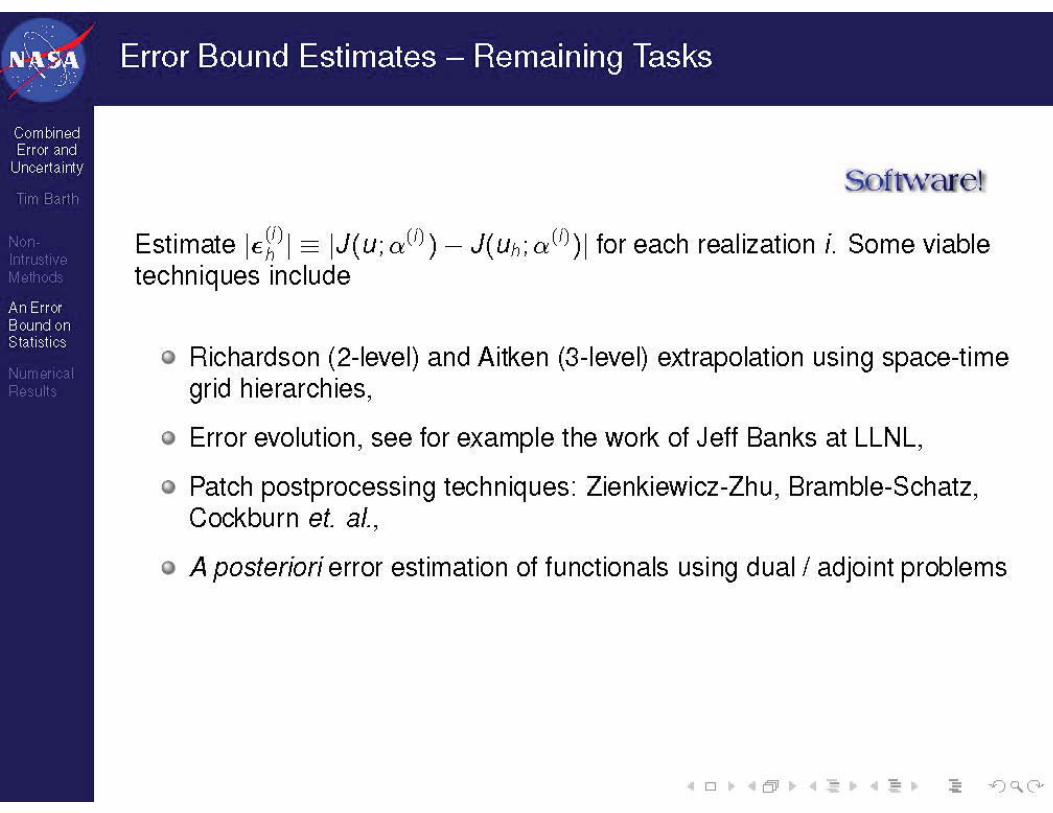
Estimate IE~) I IJ( u; aU))- J( uh; aU))I for each realization i. Some viable techniques include

o Richardson (2-level) and Aitken (3-level) extrapolation using space-time grid hierarchies,

o Error evolution, see for example the work of Jeff Banks at LLNL,

o Patch postprocessing techniques: Zienkiewicz-Zhu, Bramble-Schatz, Cockburn et. a/.,

o A posteriori error estimation of functionals using dual I adjoint problems

Further Numerical Results

.. . 1.>(_·

N\~S-1'. A Model POE Problem with Uncertainty and Error Specification • • • ... .:1 ' ••

' . ..:." ''

Combined Error and

Uncertainty

An Error Bound on Statistics

Deterministic Burgers' Problem: Viscosity-free Burgers' equation

a a at u(x, t) + ax ( u2 (x, t)/2) = 0 , (x, t) E [0, 1] x [0, T]

with sinusoidal initial data u(x, 0) = sin(21rx) .

Phase Uncertain Burgers' Problem: Introduce a random variable, w

a a 2 Otu(x,t,w) + ax(u (x,t,w)/2) =0, (x,t,w) E [0, 1] x [0, T] xP

with phase uncertain initial data

u(x, O,w) = sin(21r(x + g(w)))

o g(w) = sin(27rw)/10 in present calculations,

o Probability density, p(w): Gaussiana-=3 (p, = O,o- = 0.07),

o WENO finite-volume (cubic polynomials) used in numerical calculations,

o Glenshaw-Curtis Adaptive Polynomial quadrature used for statistics, M = 9,

o An exact solution is readily obtained, u(x, t,w) = u(x + g(w), t) for use in specifying the exact realization error .

! .. " ~ o o 0 u

~ i

physical spac·e coordinate

Solution contours at time t = .35 0.7 ·· ················-··················· ··· ··· ···································· ··· ··· ·····-······························ ··· ·························

u.~

li.4

r.-.3 ., .!:! 0.2

~ 11. 1 ;; a; "

0.0

~ -fi. 1

" i5 _,._ ? "' v ·-

-11.3

- 0.4

-fUi

-0.7 · ···································· ·········································· ············-····························· ····························· o.o 0 . 1 0 . 2 0.2 oA o.s o.6 o.7 o.e. o.s -.. c

Physical Space Coordinate

Moment statistics at timet e= .3~

~

"'

O.Dl

~ 0.0001

" ~ 1e-06

0

- mean error bourul estimate, HYGAP -- mean error, HYGAP

02 OA OJ OJ Physical Space Coordinate

- variance error bourul estimate, HYGAP -- variance error, HYGAP

0.01

-"' -~ ., 0.0001 " .~ ~

1e-06

location

1e-08

0 02 OA OJ OJ Physical Space Coordinate

Figure : Exact and estimated error bounds for the variance statistic calculated using a Glenshaw-Curtis Adaptive Polynomial (HYGAP) approximation ( M = 9) at Glenshaw-Curtis quadrature points for the Burgers' equation problem with phase uncertain initial data at time t = . 35 .

Semilinear form B(-, -)and nonlinear J(}

Primal numerical problem: Find uh E Vh such that

B(uh, wh) = F(wh) v wh E Vh-

Linearized auxiliary dual problem: Find <P E V such that

B(w, <P) = J(w) V wE V.

J(u) - J(uh) = J(u - uh)

= B(u- uh, <P)

= B(u - Uh, <P - 7rh<P) = B(u, <P- 7rh<P) - B(uh, <P- 7rh<P) = F(<P- 7rh<P)- B(uh, <P- 1rh<l>),

Final error representation formula:

(mean value J)

(dual problem)

(Galerkin orthogonality)

(mean value B)

(primal problem)

Example: Euler equation flow past multi-element airfoil geometry. M === .1, so AOA.

equivalent uniform lift coefficient lift coefficient refinement refinement

(error representation) (error control) 5.156 ± .147 5.275 ± .018 5.287 ± .006 5.291 ± .002

... 1: 40 ·u

5.7 r

5.5

~ 5.1 ' 0 u

~ 4.9

5.156 ± .346 5.275 ± .076 5.287 ± .024 5.291 ± .007

Increasing levels of adaptlvlly

- Error representation formula Error control estimate

4.7 ..

~ 5.2923

4.5 L_ .l '--'

4000 9000 14000 19000 24000 #elements

level 0 1 2 3

Error reduction during mesh adaptivity

#elements #elements 5000 5000 11000 20000 18000 80000 27000 320000

Adapted mesh (18000 elements)

The inflow angle of attack (AOA) is then assumed uncertain with truncated Gaussian probability density, AOA = Gaussian4cr ( m = 5°, u = 1 o).

Let

denote the errors in approximated expectation and variance, respectively using Glenshaw-Curtis quadrature (M=9).

level #elements E[J(uh)] V[J(uh)] LlME[J(uh)) LlM V[J(uh)] 0 5000 5.145 .01157 .147 .05619 1 11000 5.274 .01188 .018 .00462 2 18000 5.286 .01191 .006 .00240 3 32000 5.292 .01192 .005 .00148

Table : Approximated statistics and error bounds for the aerodynamic lift coefficient functional. Tabulated are the computed estimates of expectation and variance together with error bounds.

o Compressible Navier-Stokes CFD calculation,

o 2-equation turbulence model,

o Inflow Mach number uncertainty, Moo = Gaussian3a-(m = .84, u = .02)

o Angle of Attack uncertainty, AOA = Gaussian3a- ( m = 3.06, u = .075)

o Hybrid Glenshaw-Curtis Adaptive Polynomial quadrature (M=9 x 9).

I~ I

expectation (density) log 10 variance(density) ~ D CJil = -::_ I ~ ·t)~(>-

• Moment statistics have a limited value whenever the output PDF departs strongly from a normal distribution.

-L5ir====r:=:=::r:::===:r===:::::;:==;::::::=:;==::::;:::=j -1. 4

-1.3

-1. 2

-1. 1

-1. 0

-0 .9

-0.8

..... -0 .7

" -~ -0 6 . ·- - -·-~ ·····-·.-..;'

;;::: -0 5

~ .a: 4 I -- <- -·-·->······-·- ->···- ·······-+--····""' v

:v-0. 31~ .~ ];;..~~ijlii ~ -0. 2

~ -0 .1 .. "- o.o l ~.r-""'+· . , .. ,.. ·+ . ·'-· .. , .. +···' ···c

0.1

0 . 2

0.3

o. • I - --+-·····-·-·-· :-·-·---·····-·: ---·····-·---" ··-·-·---··· ;--····-·-·-···:·-·---·····-+-·····-·--· :··-·-·-·-···-·: ---·······-·-'····-·-·---··· :· - - I 0.5 ............. ; . ; ; ' · >- ; ............. ; -> ; ;. . .... .

0.6llt +············· ...... ;... ··+·············-···········-' .......... +···················-'·············' ·····················!

0.711 --····'-·····-·-- ······-······· >--······--" ····--··· ···-····-·--·· ···--········-'-·····-·-- -·····--····· ··-·················-·-···

o~ o~ o~ o~ oe oro o~ oM o~ ooo oE 1.00 X

1.0 0

0.95

0.90

0 .85

0 .80

0 . 75

0.70

0.65

0.60

0.55

0.50

0.45

0.40

0.35

0 .30

0 .25

0.20

0 .15

0.10

0.05

0.00

PDF and Quantiles at span=.65 (left)

Ongoing work:

4.75

4.50

4.25

4.00

3.75

3.50

E 3.2s

" ·u J.oo

~ 2.75 0 v ~I 2.50

~ 2.25

"' e 2.oo "-'u:' 1.75

" Q. 1.50

1.25

1.00

0.75

0.50

0.25

0.00

, ............ 1.- PDF, x - 0. 705 · · · J-lO% p,obabmty .... J

- d - - ~ -

. .......... , j . .. __ ...........

•

\ [ I

1\ I

1\ 1 I J

/ i··-·-···· j

; ........ \ ····-·-· j , ....... 1'---... ~

{~ l -0.85 -0 .80 -0 .75 ·0 .70 -0.65 -0.60 -0.55 -0 .50 -0 .45 -0 .40 -0.35 -0.30 -0 .25

pressure_coefficient

Bi-modal PDF at x=.705 (right)

g Calculation of non-moment statistics, e.g. PDFs, quantiles, etc.

Q Error bounds for non-moment statistics.

1.00

0 .95

0 .90

0 .85

0 .8 0

0 .75

0.70

0 .65

0 .60

0 .55

0 .5 0

0 .45

0.40

0 .35

0 .30

0 .25

0 .20

0 .1 5

0.10

0 .05

0 .00

Quantifying the effect of realization error in the calculation of output moment statistics is a novel new capability not found elsewhere.

The Adaptivity Framework and software API opens exciting new possibilities in adaptive CFD calculations.

Moving beyond moment statistics towards the estimation of error bounds for more general statistical measures and PDFs is a vitally important capability that must be provided in order that UQ is genuinely useful to engineers.