1

Tidal and residual currents over abrupt deep-sea topography based on shipboard ADCP data and

tidal model solutions for three popular bathymetry grids.

Christian Mohn (1), Svetlana Erofeeva (2), Robert Turnewitsch (3), Bernd Christiansen (4), Martin

White (5)

(1) Department of Bioscience, Aarhus University, Roskilde, Denmark

(2) College of Earth, Ocean and Atmospheric Sciences, Oregon State University, Corvallis, USA

(3) The Scottish Association for Marine Science, Scottish Marine Institute, Oban PA37 1QA, UK

(4) Institut für Hydrobiologie und Fischereiwissenschaft, Universität Hamburg, Zeiseweg 9, D-

22765 Hamburg, Germany

(5) Earth and Ocean Sciences, School of Natural Sciences, National University of Ireland, Galway,

Ireland

Abstract

The response of tidal and residual currents to small scale morphological differences over abrupt

deep sea topography (Seine Seamount) was estimated for bathymetry grids of different spatial

resolution. Local barotropic tidal model solutions were obtained for three popular and publicly

available bathymetry grids (Smith and Sandwell TOPO8.2, ETOPO1 and GEBCO08) to calculate

residual currents from vessel mounted Acoustic Doppler Current Profiler (VM-ADCP)

measurements. Currents from each tidal solution were interpolated to match the VM-ADCP

ensemble times and locations. Root mean square (RMS) differences of tidal and residual current

speeds largely follow topographic deviations and were largest for TOPO8.2 based solutions (up to

2.8 cm s-1) in seamount areas shallower than 1000 m. Maximum RMS differences of currents

obtained from higher resolution bathymetry did not exceed 1.7 cm s-1. Single depth-dependent

maximum residual flow speed differences were up to 8 cm s-1 in all cases. Seine Seamount is

located within a strong mean flow environment and RMS residual current speed differences varied

between 5 and 20 % of observed peak velocities of the ambient flow. Residual flow estimates from

shipboard ADCP data might be even more sensitive to the choice of bathymetry grids if barotropic

tidal models are used to remove tides over deep oceanic topographic features where the mean flow

is weak compared to the magnitude of barotropic tidal, or baroclinic currents. Realistic topography

and associated flow complexity are also important factors for understanding sedimentary and

ecological processes driven and maintained by flow-topography interaction.

2

Keywords

Flow-topography interaction; OSU inverse tidal model; shipboard ADCP; global bathymetry grids;

Seine Seamount; GEBCO08; ETOPO1; Smith and Sandwell TOPO8.2

1. Introduction

Our picture of the deep-ocean seafloor landscape has constantly improved over the past decade. The

combination of satellite gravimetry, in-situ ship soundings and processing techniques produced an

unprecedented view of the true complexity of the seafloor (Smith and Sandwell 2004). It also

provides researchers with highly valuable global data products to better understand oceanic

processes at spatial scales and resolution not previously available. Most of the data are regularly

updated by results from seabed surveys and are made publicly accessible by various national and

international databases (see http://www.gebco.net/links/ for an overview). Seamount research has

strongly benefited from improved seafloor bathymetry and has substantially progressed as a

consequence. Satellite derived and ship-track bathymetry based estimates of the global distribution

of seamounts has been subject to a number of more recent studies. Depending upon data resolution,

methodology and definition of seamount attributes, projected numbers of tall seamounts > 1 km

vary from 34000 (Hillier and Watts 2007; Yesson et al. 2011) to > 105 (Wessel et al. 2010). In

contrast, less than 300 seamounts have been systematically studied in enough detail to understand

linkages between seamount dynamics, ecosystem functioning and ecology (e.g. Genin 2004; Clark

et al. 2010; Etnoyer et al. 2010). This discrepancy is not surprising considering the significant

advances in remote sensing and seabed mapping technologies over the past two decades in

comparison with the logistical constraints of site specific surveys.

Seamount-flow interactions generate a large variety of processes which can coexist over a wide

range of spatial and temporal scales. Knowledge of the spectrum of physical processes and their

dependence on the local physical environment (e.g. ambient stratification, latitude, seamount height

and tidal dynamics) is well-established through a robust foundation of available case studies. It is

largely built upon a combination of theoretical concepts, in-situ hydrographic and current

measurements at individual locations and bio-physical modeling efforts (e.g. Lavelle and Mohn

2010). Only few studies are available, however, describing the spatial variability of the larger scale

residual flow within and immediately outside the direct sphere of influence of seamounts (e.g.

Codiga and Eriksen 1997). Such information is an important prerequisite to understand patterns and

mechanism of entrainment and downstream advection of biological and sedimentary material in the

3

wider context of seamounts as conduits for bio-connectivity and large-scale transport of constituents

(Genin and Dower 2008; Mohn and White 2010). Vessel mounted Acoustic Doppler Current

Profilers (VM-ADCPs) are potentially useful observational tools to provide such information at a

high spatial resolution over a comparatively large area. VM-ADCP data contain a large spectrum of

oceanic motions and removing barotropic tidal currents is one essential post-processing step to

extract the sub-tidal residual flow. In the case of seamounts, de-tided VM-ADCP data is expected to

contain signatures of locally generated flow phenomena, e.g. tidally rectified flow, inertial currents,

high-frequency trapped and internal waves. However, high-frequency motions cannot be adequately

resolved in VM-ADCP data due to the inherent space-time aliasing. Residual flow therefore, refers

to the oceanic flow spectrum after removal of barotropic tides. Several VM-ADCP de-tiding

procedures are well documented in the literature. The preferred methodology largely depends on the

tidal and geomorphological characteristics of the sampling area and the design of the sampling grid.

Commonly used de-tiding procedures include (i) least squares tidal fitting and spatial interpolation

techniques directly applied to the VM-ADCP measurements (e.g. Candela 1992; Münchow 2000),

(ii) systematic and repeated surveys covering multiple tidal cycles (e.g. Valle-Levinson and

Matsuno 2003; Flagg et al. 2006), (iii) predictions from numerical tidal models (e.g. Pickart et al.

2005) and (iv) tidal solutions based on combinations of various techniques (e.g. Carillo et al. 2005).

Erofeeva et al. (2005) provide a short introduction into benefits and problems of the most common

techniques (i) and (iii). An overview of differences between standard de-tiding techniques is given

in Foreman and Freeland (1991) and Isobe et al. (2007).

Our study highlights the importance of different bathymetry grids for obtaining local tidal currents

from a barotropic tidal model and subsequent analysis of the VM-ADCP measurements. More

specifically, our paper compares tidal and residual currents from VM-ADCP measurements by

using local barotropic tidal solutions of the OSU (Oregon State University) inverse tidal model

based on three popular and publicly available bathymetry grids (GEBCO08, ETOPO1, TOPO8.2).

Accurate bathymetry has been identified as one of the key factors for the reliability of tidal

modeling in areas of highly variable bottom topography (Erofeeva et al. 2003). The results will be

discussed in the context of wider implications for sub-mesoscale dynamics and associated

biophysical coupling. We focus on Seine Seamount, an isolated seamount in the subtropical NE

Atlantic and subject to a multi-disciplinary study within the EU FP5 OASIS project (Christiansen

and Wolff 2009). The paper is organized as follows. Study site, data and methods are described in

section 2. A comparison of tidal and VM-ADCP residual currents obtained from different barotropic

tidal solutions is presented in section 3. Finally, possible implications for understanding and

interpreting flow and sediment dynamics and its relevance to different aspects of seamount ecology

4

are discussed in section 4.

2. Study site, data and methods

2.1 Study site and physical setting

Seine Seamount is a tall, conically shaped seamount located in the subtropical NE Atlantic northeast

of the island of Madeira (Fig. 1a). It rises sharply from abyssal water depths > 4000 m towards a

summit depth of 170 m. Seine Seamount is located at the eastern boundary of the Azores Current

(AC) which forms one southeastward branch of the North Atlantic subtropical gyre. The AC is one

of the most distinctive flow features of the basin-wide upper ocean circulation in the subtropical NE

Atlantic. Based on results from Klein and Siedler (1989) and Lozier et al. (1995), Jia (2000)

defines the AC as a 60 – 100 km wide meandering jet moving southeastward with velocities of 25 –

50 cm s-1 in the upper few hundred meters east of the Mid-Atlantic Ridge between the Azores and

Madeira Islands. Its central axis is located roughly along 35° N latitude. The AC has been identified

as a highly dynamic region of intense eddy activity along its zonal boundaries as a result of

baroclinic instabilities of the main AC jet (e.g. Alves et al. 2002; Sangrà et al. 2009). At greater

depths, southwestward propagating high saline Mediterranean Water eddies (Meddies) have been

frequently observed (Richardson et al. 2000). Topographic modulation of Meddies through

seamounts is a common phenomenon in the area and well documented in a number of studies (e.g.

Shapiro et al. 1995; Wang and Dewar 2003). Bashmachnikov et al. (2009) reported Meddy collision

and temporary trapping events at Seine Seamount. The impact of seafloor topography on the

lifetime and passage of Meddies is only one example that highlights the importance of seamounts

and other submarine features (such as ridge systems and submarine banks) for interior ocean

dynamics and energy transfer. It has been demonstrated that deep-ocean topographic features are

important conduits for water mass and material transport over a wide range of spatial and temporal

scales (e.g. McGillicuddy et al. 2010; Mohn and White 2010; Kunze and Llewellyn Smith 2004).

2.2. Bathymetry grids and tidal model solutions

Our main aim is to investigate the modulation of modelled barotropic tidal currents and VM-ADCP

residual flow estimates based on bathymetry grids of different spatial resolution in a small oceanic

area with abrupt topographic changes. For this purpose we use three data sets accessible in the

public domain. The key attributes of each grid and main literature references are summarized in

Table 1. TOPO8.2 is a 2 arc-minute version of the Smith and Sandwell (1997) bathymetry. Although

5

somewhat outdated, TOPO8.2 is a useful reference grid in the context of this study (after

completion of this study, version TOPO15.1 of the Smith and Sandwell bathymetry was released).

ETOPO1 provides ocean bathymetry on a 1 arc-minute grid and is mainly built upon the Smith and

Sandwell (1997) bathymetry in ice free oceanic regions equatorward of 80° latitude. ETOPO global

relief models integrate land topography and ocean bathymetry from various regional and global data

sets. They are assembled at and available from the National Geophysical Data Center of the

National Oceanic and Atmospheric Administration (NOAA). The GEBCO08 bathymetry (General

Bathymetric Charts of the Oceans; British Oceanographic Data Centre 2009) has a resolution of 30

arc-seconds and includes TOPO11.1, a newer version of the Smith and Sandwell (1997) bathymetry

complemented by a large database of bathymetric soundings. A grid comparison of the Seine

Seamount morphology reveals significant differences (Fig. 2). The basic shape and outline of the

seamount are similar in all grids, but many of the small-scale slope and depth variations visible in

the finer-scale grids are not present in the TOPO8.2 morphology. The ETOPO1 and GEBCO08

grids also differ considerably in both bottom slope and bathymetric detail, but over much shorter

spatial scales. The largest variations between grids occur over the seamount summit and along the

southeastern seamount rim (Fig. 2 d).

The OSU tidal inversion software (OTIS) is used to obtain local solutions of barotropic tidal

currents. The model is described in detail by Egbert and Erofeeva (2002). The model domain covers

the area between 13°W – 16°W in longitude and 32°N – 35°N in latitude with Seine Seamount in its

center (see black square in Fig. 1 a). The grid size is 360 x 360 with a uniform grid spacing of 30

arc-seconds (1/120°) corresponding to the highest bathymetric resolution (GEBCO08) used in this

study. The quality of barotropic tidal current estimates from tidal models largely depends on model

resolution, accuracy of the bathymetry grid and boundary conditions (e.g. Padman and Erofeeva

2004). Therefore, the coarser bathymetry grids (TOPO8.2, ETOPO1) were interpolated to fit the 30

arc-seconds model grid node locations. Eight tidal harmonics (M2, S2, O1, K1, N2, K2, P1, Q1) are

computed as direct factorization solutions for each bathymetry grid without applying an area-

specific data assimilation. The open boundary conditions are taken from an existing regional OTIS

solution for the Atlantic Ocean (AO_2008, 1/12°) which integrates various assimilated altimetry

and in-situ data products.

6

Bathymetry grid TOPO8.2 (2001) ETOPO1 (2008) GEBCO08 (2009)

Spatial resolution 2 arc-minutes 1 arc-minute 30 arc-seconds

Main data source

equatorward of 80°

latitude

Smith and Sandwell

grid, version 8.2 –

satellite gravimetry,

bathymetric soundings

Smith and Sandwell

grid, version not

specified – satellite

gravimetry,

bathymetric soundings

Smith and Sandwell

grid, version 11.1 –

satellite gravimetry,

bathymetric soundings

Main references Smith and Sandwell

(1997)

Amante and Eakins

(2009), Smith and

Sandwell (1997)

Smith and Sandwell

(1997), GEBCO (2009)

Online access Satellite Geodesy,

Scripps Insitution of

Oceanography,

University of

California San

Diego(http://topex.ucsd

.edu/)

National Geophysical

Data Centre, NOAA

(http://www.ngdc.noaa.

gov/mgg/global/global.

html)

British Oceanographic

Data Centre on behalf of

GEBCO

(http://www.gebco.net/)

Table 1: Key attributes and main literature references of the bathymetry grids used in this study.

2.3. VM-ADCP data

VM-ADCP data were collected at Seine Seamount onboard RRS Discovery during the period 15-22

July 2004 as part of a multi-disciplinary survey within the framework of the EU FP5 OASIS project

(see cruise track in Fig. 1b). On-station and underway velocities were collected with a 75 kHz

Teledyne RD Instruments Ocean Surveyor system mounted in the ship's hull along with positioning,

heading and time data. The instrument was configured to sample at a bin length of 16 m (first bin at

29 m) with a total sampling range of 60 bins (973 m). Prior to post-processing, single ping ENS

velocity profiles (RDI Ocean Surveyor raw data including basic error screening and navigation)

were time averaged to obtain two data sets of 2 and 5 minute ensembles for later comparison. The

Common Oceanographic Data Access System (CODAS) was used for data processing. CODAS is a

comprehensive ADCP data post-processing toolbox developed and maintained at the University of

Hawaii (Firing et al. 1995; http://currents.soest.hawaii.edu/docs/adcp_doc/index.html). Post-

processing was carried out for both the 2 and 5 minute ensemble averaged data sets according to

7

procedures recommended by Hummon and Firing (2003) and Firing and Hummon (2010). An

initial transducer misalignment check was performed to obtain a first estimate of transducer

orientation relative to the ship's heading by comparing single ping velocities at each beam. This

procedure did not indicate any unusual and large transducer misalignments. A quality control of

ensemble profiles was performed afterwards to retain velocity profiles/bins not affected by ship

induced turbulence, object interference and bottom reflection. A water track calibration was then

made to obtain best estimates for the transducer amplitude scale factor and transducer orientation

relative to the ship's heading. For this procedure, bins 5 – 20 (93 – 333 m depth range) were taken

as the oceanic reference layer, thus avoiding short-term variability caused by ship-induced

turbulence and weather events. The resulting correction factors for transducer orientation (phase)

and amplitude were found to be 2.3° and 1.005 respectively. After applying the correction factors,

the calibration procedure was repeated to verify any remaining transducer misalignment. The

resulting phase angle was 0.26° and no further correction was carried out. Finally the navigation

calculation of the ship's position and speed was carried out to obtain best estimates for ship velocity

and to calculate absolute current velocities. The most important error sources in calculating absolute

ADCP velocities are (i) the transducer misalignment (phase) bias in the cross-track velocity

component and (ii) the velocity amplitude scale factor bias in the along-track velocity component.

Phase errors of < 0.2° and amplitude scale factor errors of < 0.5% correspond to velocity errors of 2

cm s-1 and 2 – 3 cm s-1 respectively (Firing and Hummon 2010). The instrument’s measurement

accuracy is 0.5 cm s-1 according to the manufacturer’s data.

3. Results

3.1. Along-track VM-ADCP velocities

The major features of the oceanic flow field along the cruise track (including barotropic tidal

currents) separated into its east-west (u) and north-south (v) components are shown in Fig. 3 a, b.

North of the central seamount latitude at 33.75 °N (Fig. 3 c), the flow is predominantly

southeastward with peak velocities varying between 25 cm s-1 and 35 cm s-1. This jet-like flow

extends from the surface down to 600 m water depth. South of the seamount, the flow in the upper

600 m is considerably weaker with maximum velocities not exceeding 15 cm s-1. The significant

change of the flow pattern between days 194 and 195 is the result of a temporary survey

interruption due to logistical reasons. The difficulty of putting our observations into the context of

previous measurements in the region lies in the limitation of our sampling area and period.

Observations in the eastern recirculation region (east and south of Madeira) where the AC extends

8

southward into the Canary Current (CC) often demonstrate a dominance of variable over mean flow

conditions. The strongest sub-tidal variability occurs at periods of 1 – 3 months (Siedler and Onken

1996), but can be higher in regions of long-lived eddy corridors (Sangrà et al. 2009). In a recent

analysis of the long-term surface circulation of the AC system based on 17 years of re-gridded

drifter and altimetry data, the mean flow east of Madeira appears as a mean southward flow with

maximum speeds of 3 - 5 cm s-1 (Barbosa Aguiar et al. 2011). These values are one order of

magnitude smaller than our observed velocity maxima. In contrast, instantaneous VM-ADCP

measurements by Pelegrí et al. (2005) in the CC region at around 31°N and east of 14°W revealed

currents of up to 50 cm s-1 in the uppermost layers. A one week (14. - 21. July 2004) composite of

gridded (1/3°) absolute geostrophic surface currents from AVISO satellite altimetry

(www.aviso.oceanobs.com) suggests typical current speeds in the seamount region to be closer to

values observed by Pelegrí et al. (2005). These discrepancies indicate that the region east and

southeast of Madeira is dominated by transient and energetic eddy activity which is under-

represented in long-term averages. The AVISO data set was also used for a qualitative comparison

with near-surface (top 60 m) gridded VM-ADCP currents from our seamount survey (Fig. 4). The

VM-ADCP data gridding procedure is described in more detail in the next section. This comparison

shows that the VM-ADCP currents are largely comparable (both in flow direction and magnitude)

with the AVISO currents from the same period. The high-resolution VM-ADCP currents indicate a

local modulation of the flow field close to the seamount which is not visible in the AVISO data and

masked by the coarser resolution of the AVISO grid. The resemblance with the AVISO data

provides reasonable confidence in the ADCP currents as a realistic snapshot of the circulation at and

close to Seine Seamount. Remaining differences originate from tidal signals in the ADCP velocity

fields and uncertainties in the ADCP velocity estimates, as described in section 2.3.

3.2. Comparison of barotropic tidal currents

In this section we describe the differences between the total barotropic tidal currents obtained from

each bathymetry grid. Tidal model solutions were extracted at all 2 minute VM-ADCP ensemble

profile times and locations. These currents are used for later de-tiding of the VM-ADCP data. Tidal

solutions based on the GEBCO08 bathymetry are taken as a reference to introduce the main

properties of the along-track barotropic tidal current field in relation to bottom depths (Fig. 5 a).

Tidal current amplitudes away from the seamount vary between 2 and 3 cm s-1. The largest

contributor is the principal semi-diurnal component M2 consistent with previous observations in the

eastern North Atlantic (e.g. Siedler and Paul 1991). Tidal currents are generally amplified over the

seamount with peak values of up to 13 cm s-1. The best agreement between tidal currents from

9

different tidal model solutions is found in the deep waters away from the seamount. Above the

seamount, ETOPO1 and GEBCO08 based tidal currents are comparable in magnitude, but vary in

areas where resolution becomes important to resolve abrupt along-track changes of the topographic

slope (Fig. 5 a, b). TOPO8.2 based tidal currents differ significantly at shallower seamount

locations, where seamount height and slope are often underrepresented in comparison with

GEBCO08 and ETOPO1 characteristics (Fig. 5 c). As a consequence, magnitudes of TOPO8.2

based tidal currents are lower over most of the sampled seamount area.

The spatial modulation of modelled barotropic tidal currents by different seamount bathymetries

was analysed after horizontally re-gridding the VM-ADCP along-track tidal currents. Each data set

was mapped to a uniform 30 arc-seconds grid to match the highest bathymetric resolution

(GEBCO08) by applying a cubic spline interpolation. Tidal ellipses of the major diurnal and semi-

diurnal constituents M2 and K1 at characteristic seamount locations are shown in Fig. 6 a and b.

ETOPO1 and GEBCO08 based M2 and K1 tidal ellipses are similar over most of the area, except for

the northern summit region, where inclination, eccentricity and magnitude can vary considerably.

Here, GEBCO08 tidal currents are typically 4 cm s-1 (M2) and up to 1 cm s-1 (K1) higher than

corresponding values from ETOPO1 solutions. Magnitudes of TOPO8.2 based tidal currents are

consistently lower at corresponding seamount locations. The most pronounced exception is a strong

amplification of the TOPO8.2 based K1 tidal current over the central seamount region. This is not

visible in the other solutions and is most likely a consequence of the summit misrepresentation in

the TOPO8.2 seamount morphology. The tidal amplification above the seamount relative to the far

field varies with local bottom depth and for individual tidal constituents. The strongest relative

amplification of the four major tidal constituents over the seamount was found to be 6 (M2), 2 (S2),

7 (K1), and 2 (O1) respectively.

Pairwise differences of the total barotropic tidal current speed ∆UTide (����� = ������ + ����� ) are

shown in Fig. 7 a – c , together with the corresponding 500 m and 2000 m depth contours of each

bathymetry grid. TOPO8.2 tidal currents generally underestimate other tidal solutions across the

northern seamount region inside the 500 m isobath (Fig. 7 a, b). GEBCO8 and ETOPO1 tidal

solutions predict current speeds of more than 4 cm s-1 higher than TOPO8.2 solutions. The opposite

effect, i.e. stronger TOPO8.2 based tidal currents, occurs further south where the actual seamount

summit is located in the TOPO8.2 grid (Fig. 7 a, b). The best agreement, both in seamount

morphology and tidal current speed, is found between GEBCO08 and ETOPO1 based tidal

solutions. Differences between GEBCO08 and ETOPO1 tidal currents are generally small (|∆UTide|

10

< 1 cm s-1) outside the 500 m isobath except for the southeastward seamount extension predicted by

the GEBCO08 bathymetry, where GEBCO08 based tidal current speeds are up to 4 cm s-1 higher

(Fig. 7 c). Inside the 500 m isobath, however, tidal current speed variations are much smaller and

within the range ∆UTide = ± 2 cm s-1. Standard deviations of all three solutions are shown in Fig. 7 d

confirming that relative errors are highest along the northern summit area and in regions of abrupt

changes in slope or strong morphological differences.

3.3. Comparison of residual currents

Residual currents were calculated by removing the barotropic tidal velocity components (uTide,vTide)

from the corresponding VM-ADCP velocity components (u,v) at each 2 minute ADCP ensemble

profile location and depth bin along the cruise track. The resulting flow components (uRes=u-uTide,

vRes=v-vTide) were spatially interpolated following the same procedure as for the tidal currents prior

to calculating the residual flow speed differences ∆URes. Figs. 8 a – c show the ∆URes fields averaged

over the top 200 m of the water column for all combinations of modelled tidal currents. The largest

differences (|∆URes| ≥ 4 cm s-1) are again obtained for combinations involving TOPO8.2 tidal

currents (Fig. 8 a, b) whereas typical values of ∆URes are ± 3 cm s-1 for residual flows based on

GEBCO08 and ETOPO1 tidal currents. Residual flow speed differences are spatially less

homogenous and not directly linked to barotropic tidal current differences. In addition to

bathymetry, additional factors such as the presence of baroclinic flow and signatures of inertial

currents and internal tides may equally be important for spatial variations of the de-tided flow field.

The overall variability pattern of all residual flow speed data is again dominated by strong

variations in seamount regions where bathymetric characteristics differ most (Fig. 8 d).

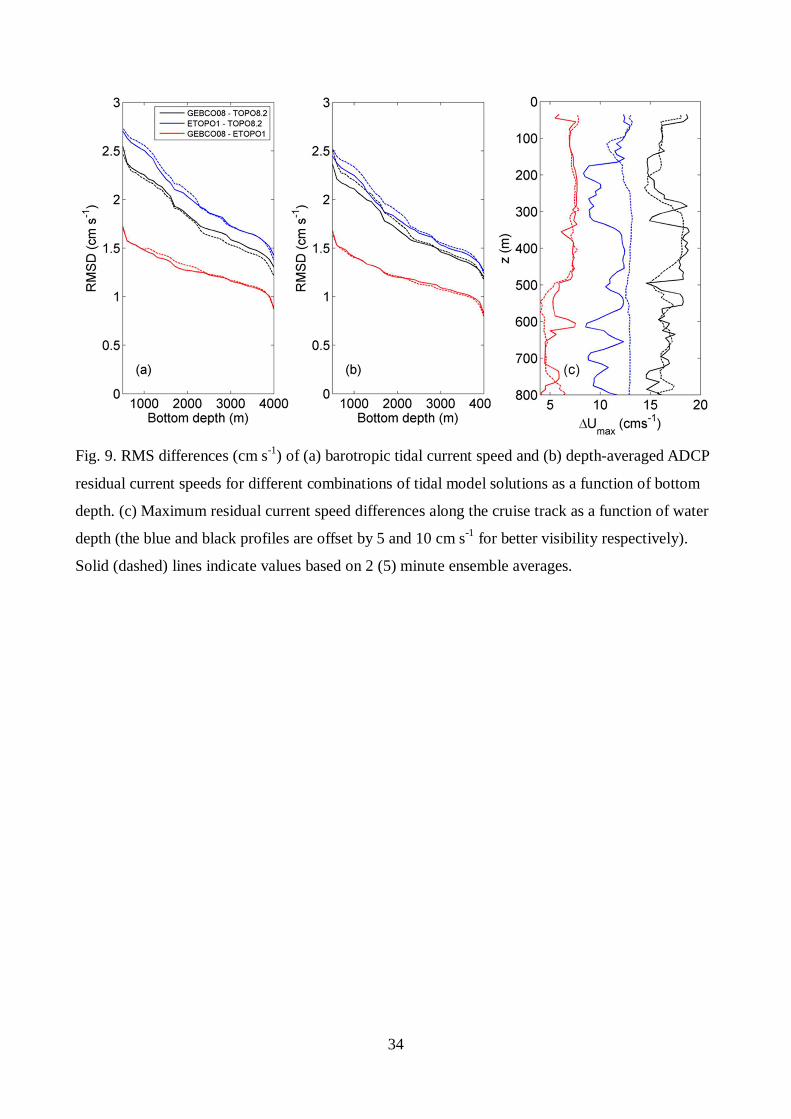
The importance of bathymetric detail and associated tidal response for determining residual flow

characteristics is further demonstrated in Fig. 9. Pairwise RMS differences of both the depth-

averaged residual and tidal current speeds were calculated for all combinations of tidal solutions

and bathymetry grids. The calculation was carried out for un-gridded along-track VM-ADCP and

tidal currents for bottom depth intervals ∆H = 100 m within the depth range 500 m to 4000 m

according to:

� �(��, ��) = �� (��,� −��,�)������ 1��

where Ui and Uj are the residual and tidal flow speeds based on different tidal solutions i and j (i, j =

1:3, i ≠ j) and N∆H is the number of data points per bottom depth range ∆H. Tidal and residual flow

11

speed RMS differences (Fig. 9 a, b) between coarser (TOPO8.2) and finer (ETOPO1, GEBCO08)

grid based tidal solutions increase by almost a factor of two from abyssal waters (1.3 cm s-1)

towards the shallower and steeper seamount areas at bottom depths 500 m < H < 1000 m (> 2.3 cm

s-1). The larger differences in these shallower seamount areas mainly arise from insufficient

accuracy of important seamount characteristics in the TOPO8.2 grid. Thus, the spatio-temporal

variation of TOPO8.2 based tidal currents is not adequately represented. Corresponding residual

and tidal flow differences between GEBCO08 and ETOPO1 solutions vary at a much lower level

with RMS errors between 0.8 and 1.7 cm s-1.

The highest observed differences !�"#$ (%) = max)*��(%) −��(%)*+ occurring at least once over

the sampling period at each VM-ADCP depth bin is shown in Fig. 9, with i and j being different

tidal solutions (i, j = 1:3, i ≠ j) and z being the water depth of each vertical ADCP bin. ∆Umax values

are between 5 and 8 cm s-1 for all combinations of tidal model solutions. Thus, depth-dependent

single maximum residual current speed differences are at least a factor of 2 higher than the RMS

differences. It is interesting to note that these single maximum differences along the cruise track do

not vary strongly with water depth. They are highest at seamount summit depths, but do not

substantially decrease towards deeper seamount regions.

An important aspect of ADCP post-processing is ensemble averaging, more specifically the period

over which single ping velocity profiles are averaged to obtain one ensemble profile. Ensemble

averaging over a longer period reduces the impact of measurement errors, but also reduces the

spatial representation and resolution of ensemble profiles. We estimated the potential influence of

ensemble averaging by re-processing the ADCP data set at 5 minute ensemble averages, more than

double of our initial averaging period. Residual currents were then calculated by re-sampling the

modelled barotropic tidal currents at the 5 minute ensemble times and locations for all bathymetry

grids. The resulting RMS differences are shown as dashed lines in Fig. 9. Tidal and residual flow

RMS differences are similar in magnitude indicating that the error from ensemble averaging is

small in comparison with variations introduced by spatial resolution effects of different bathymetry

grids. Longer period ensemble averaging does also not critically impact on the maximum

differences at each ADCP bin. ETOPO1/TOPO8.2 differences are the only exception, where 5

minute ensemble averaging causes systematically increased ∆Umax values across the whole water

column.

12

3.4. Baroclinic currents

Ocean currents have a full spectrum of barotropic and baroclinic motions and the baroclinic motions

may well be enhanced within certain parts of the water column (e.g. Lavelle and Mohn, 2010). A

short term (7.3 day) bottom mounted ADCP deployment, located in 180 m of water depth at the

western edge of the Seine seamount summit, can be used to highlight the possible role of baroclinic

motions on the quality of the de-tiding process (Fig. 10). Here the barotropic and baroclinic signals

were separated by first calculating the barotropic current through a depth averaging of the currents

within the 4m sized bins from 118-162 m depth (the lowest 3 bins at 166,170 and 174 m not being

used as they were within the frictional benthic boundary layer, based on the Ekman veering

character of the 7.3 day mean current vectors). Baroclinic currents were then estimated after

subtraction of the calculated barotropic currents. At the M2 period, barotropic currents were

estimated to be at least and order of magnitude greater than baroclinic ones (Fig. 10 a). An increase

in the baroclinic energy was found as the seabed was approached, perhaps reflecting the interaction

of topography with the stratified tidal flow. At the inertial period (Fig. 10 b), the baroclinic current

was small at mid depths, but closer in magnitude to the barotropic signal near the seabed in the

easterly, cross-isobath, component. There is also some suggestion of an increase towards shallower

depths at the top of the deep winter thermocline (100-150 m depth) where wind induced motions

were likely to be more significant. The results, at least here for our test case, indicate that at depths

away from the strong vertical stratification or the topographic feature itself, the influence of

baroclinic components might reasonably be assumed not to contribute significant errors to the de-

tiding process. The likely enhancement of baroclinic energy close to topographic features or at any

thermocline, however, may well mean caution should be applied to any use of and interpretation

from the de-tiding from tidal model data. Of course the depth range close to the seabed is likely to

be a region of interest, but flow data here will be hard to successfully obtain given the constraints of

ADCP use close to reflecting boundaries and the problems associated with the boundary conditions

for the tidal modeling.

4. Discussion and conclusions

4.1. Bathymetry effects and seamount dynamics

The general capability of ocean models to resolve the wide spectrum of processes associated with

small-scale topographic features has been previously emphasized (e.g. Padman et al. 1999; Gille et

al. 2004). A better understanding of bio-physical processes related to flow-topography interaction at

13

seamounts and other submarine features depends on an accurate picture of their physical

characteristics. Improving the accuracy of bathymetry data in these confined areas has been

identified as a future research priority (Clark et al. 2012). Marks and Smith (2006) provided a

comprehensive evaluation of strength and weaknesses of a variety of bathymetry grids available at

the time. Our comparison of barotropic tidal and shipboard ADCP residual currents is based on

three bathymetry grids of different resolution at a tall, isolated seamount. It confirms the sensitivity

of barotropic tidal currents to different bathymetries and highlights implications for removal of tidal

flow from observed currents in areas of abrupt topographic changes. Seine Seamount is located in

an environment of strong background currents and the residual flow speed RMS differences

typically vary between 5 and 20 % of the total VM-ADCP peak velocities in regions shallower than

1000 m bottom depth depending on the respective tidal solution. Corresponding RMS differences

between barotropic tidal currents are considerably higher with values up to 35 % of the strongest

modelled tidal currents. Spatial modulations of tidal and residual currents largely follow

topographic deviations and are most pronounced at and close to the central seamount region. The

spatio-temporal analysis has one significant error source in addition to instrument and data

uncertainties. The asynoptic sampling of the seamount region adds a bias to the spatially re-gridded

residual flow fields where the largest errors occur in areas without or little data coverage, especially

between VM-ADCP track lines in areas outside the 4000 m isobath (see Fig. 1 b). Robust results

from the spatial re-gridding procedure can be expected within the central seamount region (inside

the 4000 m isobath).

Despite these challenges, our analysis indicates that detided VM-ADCP residual currents over

abrupt topographic features can vary significantly depending on the underlying bathymetry grid.

This leads to the general conclusion that VM-ADCP residual flow estimates derived by this

procedure might be even more sensitive to the choice of bathymetry grids in regions where mean

flows are weak compared to the magnitude of the barotropic tidal currents or baroclinic motions

(Fig. 10). The relationship between topographic properties and dynamical response has been

highlighted in a number of systematic modeling and laboratory studies. Modulation of the quasi-

steady far field flow over isolated topography occurs in the form of vortex formation, trapping and

shedding. The existence, residence time and shedding frequency largely depend on a combination of

impinging flow magnitude, topographic characteristics and stratification. (Boyer and Kmetz 1983;

Chapman and Haidvogel 1992; Cenedese 2002; Francis 2005). At sub-tidal periods, variations of

topographic slope and barotropic tides influence local dynamics such as tidal amplification, trapped

wave formation and internal wave dynamics (e.g., Baines, 2007).

14

4.2. Implications for sediment dynamics and seamount ecology

Sediment deposition is a crucial process controlling benthic biodiversity, biogeochemical fluxes,

distribution and growth of metal-rich mineral crusts at the seafloor, and the sedimentary record of

past environmental changes. A recent estimate suggests that the deep oceans could be structured by

~ 25 x 106 abyssal hills, knolls and seamounts, with the number of seamounts probably being > 105

(Wessel et al., 2010). It is therefore likely that such topographic features and their flow/topography

interactions have a globally relevant influence on deep-sea sediments and the associated biology,

biogeochemistry and geochemistry. Flow-topography interactions control the spatiotemporal

geometry of current fields near the seafloor. It has long been known that, through its mechanistic

link with bed shear stress, near-seafloor current speed constitutes an important controlling factor for

sediment dynamics (see, e.g., reviews by McCave (1984) and Winterwerp and Van Kesteren

(2004)). In addition, recent work towards a review of the interplay between seafloor topography,

boundary layer fluid and sediment dynamics in the deep sea suggests higher-frequency (tidal, near-

inertial) variability of current directions may play an important role in controlling the way deep-sea

sediments are formed (Turnewitsch et al., in prep.). It is therefore of general importance to

accurately capture the spatio-temporal variability of both current speeds and current directions. This

is particularly important for regions with sloping seafloor, including seamounts.

In temperate and mid latitudes much of the primary sedimenting particle flux to the seafloor

consists of ‘phytodetrital’ particles which have been shown to resuspend if near-seafloor current

velocities are around ~ 7 cm s-1 or above (see review by Beaulieu 2002). For certain locations on

the upper half of Seine Seamount the orientation, shape and dimensions of the modeled barotropic

current-vector ellipses of the two most important tidal constituents vary substantially between the

three different bathymetric datasets (Fig. 6). These differences are also reflected in the spatial

distributions of the total barotropic tidal current velocities, with local differences reaching up to

more than 4 cm s-1. Maximum local differences between the different detided flow fields are of a

similar magnitude (Fig. 8). Consequently, when it comes to predicting locations on seamount-scale

topography where pockets of inhibited sediment deposition and/or transient sediment resuspension

are likely, current velocity inaccuracies of several centimeters per second or more will constitute a

significant source of error.

Water flow can affect biological seamount communities in several ways. One particularly important

mechanism is food supply. Although part of the nutrition of the seamount fauna may depend on

local primary production and thus on vertical energy flux, several studies suggest that advective

15

processes and an enhanced supply from allochthonous food sources are more important (Hirch and

Christiansen 2010; Genin and Dower 2008; Morato et al. 2009; Vilas et al. 2009). Such fluxes are

responsible for the dense aggregations of organisms found at some seamounts (Genin 2004). The

flux of food particles, whether particulate organic matter (POM) or plankton, is determined by

particle concentration and by tidal and residual currents. De-tiding of actual current measurements

based on realistic bathymetry can help to assess long-term advective food fluxes in different parts of

the seamount. It may also explain part of the spatial variability in faunal abundance, in particular in

sessile filter feeders like cold water corals and sponges. For example, it is well established that

current is an important factor determining coral habitat (Genin et al. 1986, Bryan and Metaxas

2006; White et al. 2005). Rowden et al. (2010) suggest that a higher biomass of benthic filter

feeders at seamounts and a higher relative abundance as compared to deposit feeders can be

explained by enhanced fluxes of POM and zooplankton. Strong cross-slope tidal currents, both

barotropic and baroclinic, have been suggested to locally enhance organic matter fluxes through

vertical scattering and re-suspension at seamounts (Goldner and Chapman 1997) and smaller

features such as carbonate mounds (White et al. 2007). The effects of currents on the pelagic fauna

may be more complex. Apart from the retention potential of circular currents for passive particles at

seamounts (e.g. Beckmann and Mohn 2002), active movements of zooplankton or micronekton may

shift them to areas of different current velocities or directions. This mechanism of combined

behavioural and flow effects is suggested to help maintain pelagic populations in dynamic flow

regimes (e.g. Wilson and Boehlert 2004). Furthermore, benthopelagic fish may benefit energetically

both from areas of strong currents with enhanced food supply for feeding and from regions with

reduced flows for resting (resting-benefit hypothesis: Genin 2004).

4.3. Conclusions

Due to the snapshot character of our VM-ADCP survey, the results require a careful interpretation

regarding general arguments on wider implications. Keeping this in mind, our study comes to two

main conclusions. First and not surprisingly, bathymetry is a key factor when tidal models are used

to separate tidal and residual flow in VM-ADCP data over abrupt deep-sea topographic features.

Secondly, reliable estimates of the dynamical response at seamounts and associated biogeochemical

feedbacks are strongly constrained by bathymetric detail in combination with the need for spatially

and temporally coherent sampling strategies.Based on previous experience and the outcomes of this

study it seems that the following can be recommended. For studies that look into regionally

integrating sedimentological parameters (e.g., distributions of the particle tracer 234Th in the deep

water column: Turnewitsch and Springer 2001; Turnewitsch et al. 2008) bathymetric datasets with

16

lower spatial resolution, such as the ones of TOPO8.2 and ETOPO1, seem to be sufficient.

However, any attempts on or near seamount terrain to link, for example, sedimentary proxies of

non-deposition or erosion/resuspension to topographically controlled flow fields requires high-

resolution datasets such as GEBCO08 or even data sets obtained by ship-based swath bathymetry

(e.g., Turnewitsch et al. 2004; Peine et al. 2009). This would also very likely apply to any benthic

biogeochemical, biological and ecological sampling on seamounts.

Acknowledgements

We thank Julia Hummon and Eric Firing (University of Hawaii) for helpful support of processing

VM-ADCP data using the Common Ocean Data Access

System (CODASv.3, http://currents.soest.hawaii.edu/docs/adcp_doc/index.html). We also thank the

master and crew of the RSS Discovery. The measurements were carried out as part of the EU FP5

project OASIS (Contract no: EVK3-CT-2002-00073-OASIS). Support of RT through NERC grant

NE/G006415/1 is gratefully acknowledged. We thank two anonymous reviewers for constructive

and helpful comments.

17

References

Alves M, Gaillard F, Sparrow M, Knoll M, Giraud S (2002) Circulation patterns and transport of the

Azores Front‐Current system. Deep-Sea Res Pt II 49:3983–4002. doi:10.1016/S0967-

0645(02)00138-8

Amante C, Eakins BW (2009) ETOPO1 1 Arc-Minute Global Relief Model: Procedures, Data

Sources and Analysis. NOAA Technical Memorandum NESDIS NGDC-24.

Baines PG (2007) Internal tide generation by seamounts. Deep Sea Research Part I 54 (9), 1486-

1508. doi: 10.1016/j.dsr.2007.05.009.

Barbosa Aguiar AC, Peliz AJ, Cordeiro Pires A, Le Cann B (2011) Zonal structure of the mean flow

and eddies in the Azores Current system. J Geophys Res-Oceans 116:C02012.

doi:10.1029/2010JC006538.

Bashmachnikov I, Mohn C, Pelegrí JL, Martins A, Jose F, Machín F, White M (2009). Interaction of

Mediterranean water eddies with Sedlo and Seine Seamounts, Subtropical Northeast Atlantic. Deep-

Sea Res Pt II 56: 2593-2605. doi:10.1016/j.dsr2.2008.12.036.

Beaulieu SE (2002) Accumulation and fate of phytodetritus on the sea floor. Oceanography and

Marine Biology: an Annual Review 40:171-232.

Beckmann A, Mohn C (2002) The upper ocean circulation at Great Meteor Seamount. Part II:

Retention potential of the seamount induced circulation. Ocean Dynam 52:194-204. doi:

10.1007/s10236-002-0018-3

Boyer DL, Kmetz ML (1983) Vortex shedding in rotating flows. Geophys Astrophys Fluid Dyn

26:51–83.

Bryan TL, Metaxas A (2006) Distribution of deep-water corals along the North American

continental margins: Relationships with environmental factors. Deep-Sea Res Pt I 53: 1865-1879.

doi:10.1016/j.dsr.2006.09.006

Carillo L, Souza A, Hill AE, Brown J, Fernand L, Candela J (2005) De-tiding ADCP data in a

18

highly variable shelf sea: The Celtic Sea. J Atmos Ocean Tech 22:84- 97. doi: 10.1175/JTECH-

1687.1

Candela J, Beardsley RC, Limeburner R (1992) Separation of tidal and subtidal currents in ship-

mounted acoustic Doppler current profiler observations. J Geophys Res Oceans 97:769–788.

doi:10.1029/91JC02569

Cenedese C (2002) Laboratory experiments on mesoscale vortices colliding with a seamount. J

Geophys Res 107:3053. doi:10.1029/2000JC000599,

Chapman DC, Haidvogel DB (1992) Formation of Taylor caps over a tall isolated seamount in a

stratified ocean. Geophys Astrophys Fluid Dyn 64:31–65. doi: 10.1080/03091929208228084

Christiansen B, Wolff G (2009) The oceanography, biogeochemistry and ecology of two NE

Atlantic seamounts: The OASIS project. Deep-Sea Res Pt II 56:2579-2581. doi:

10.1016/j.dsr2.2008.12.021

Clark MR, Rowden AA, Schlacher T, Williams A, Consalvey M, Stocks KI, Rogers AD, O’Hara

TD, White M, Shank TM, Hall-Spencer JH (2010) The Ecology of Seamounts:

Structure, Function, and Human Impacts. Annu Rev Mar Sci 2010.2:253–278. doi:

10.1146/annurev-marine-120308-081109.

Codiga, DL, Eriksen, CC (1997) Observations of low-frequency circulation and amplified

subinertial tidal currents at Cobb Seamount, J Geophys Res 102(C10): 22,993–23,007,

doi:10.1029/97JC01451.

Egbert GD, Erofeeva SY (2002) Efficient inverse modeling of barotropic ocean tides. J Atmos

Ocean Tech 19:183–204. doi: 10.1175/1520-0426(2002)019<0183:EIMOBO>2.0.CO;2

Erofeeva SY, Egbert GD, Kosro PM (2003) Tidal currents on the central Oregon shelf: Models,

data, and assimilation. J Geophys Res, 108:3148. doi:10.1029/2002JC001615.

Erofeeva SY, Padman L, Egbert GD (2005) Assimilation of ship-mounted ADCP data for barotropic

tides: Application to the Ross Sea. J Atmos Ocean Technol. 22: 721–734. doi:

10.1175/JTECH1735.1

19

Etnoyer, PJ, Wood, J, Shirley, TC (2010) How large is the seamount biome? Oceanography

23(1):206–209, http://dx.doi.org/10.5670/oceanog.2010.96.

Flagg CN, Dunn M, Wang D-P, Rossby HT, Benway RL (2006) A study of the currents of the outer

shelf and upper slope from a decade of shipboard ADCP observations in the Middle Atlantic Bight.

J Geophys Res 111:C06003. doi:10.1029/2005JC003116.

Foreman MGG, Freeland HJ (1991) A Comparison of Techniques for Tide Removal From Ship-

Mounted Acoustic Doppler Measurements Along the Southwest Coast of Vancouver Island. J

Geophys Res 96:17,007-17,021. doi:10.1029/91JC01314

Francis S (2005) Flow-Topography Interactions, Particle Transport and Plankton Dynamics at the

Flower Garden Banks: A Modeling Study. Dissertation, Texas A&M University

General Bathymetric Charts of the Oceans (GEBCO) (2009) The GEBCO08 Grid, version

20091120, http://www.gebco.net

Genin A, Dayton PK, Lonsdale PF, Spiess FN (1986) Corals on seamount peaks provide evidence

of current acceleration over deep-sea topography. Nature 322: 59 – 61. doi:10.1038/322059a0

Genin A (2004) Bio-physical coupling in the formation of zooplankton and fish aggregations over

abrupt topographies. J Marine Syst 50:3–20. doi: 10.1016/j.jmarsys.2003.10.008

Genin A, Dower JF (2008) Seamount Plankton Dynamics. In: Seamounts: Ecology, Fisheries &

Conservation. Pitcher TJ, Morato T, Hart PJB., Clark MR, Haggan N, Santos RS (eds), Blackwell

Publishing Ltd, Oxford, UK. doi: 10.1002/9780470691953.ch5

Gille ST, Metzger EJ, Tokmakian R (2004) Seafloor Topography and Ocean Circulation.

Oceanography 17: 47-54. doi: 10.5670/oceanog.2004.66

Goldner DR, Chapman DC (1997) Flow and particle motion induced above a tall seamount by

steady and tidal background currents. Deep-Sea Res Pt I 44:719-744. doi: 10.1016/S0967-

0637(96)00131-8

20

Hillier, JK, Watts, AB (2007) Global distribution of seamounts from ship-track bathymetry data'.

Geophysical Research Letters, 34, L13304, doi: 10.1029/2007GL029874.

Hirch S, Christiansen B (2010) The trophic blockage hypothesis is not supported by the diets of

fishes on Seine Seamount. Marine Ecology 31:107-120. doi: 10.1111/j.1439-0485.2010.00366.x

Isobe A, Kuramitsu T, Nozaki H, Chang P-H (2007) Reliability of ADCP Data de-tided with a

Numerical Model on the East China Sea Shelf. J Oceanogr 63:135–141. doi: 10.1007/s10872-007-

0011-z

Jia Y (2000) Formation of an Azores Current Due to Mediterranean Overflow in a Modeling Study

of the North Atlantic. J Phys Oceanogr 30:2342–2358. doi: 10.1175/1520-

0485(2000)030<3C2342:FOAACD>3E2.0.CO;2

Käse RH, Zenk W (1996) Structure of the Mediterranean Water and Meddy Characteristics in the

Northeastern Atlantic. In: The Warmwatersphere of the North Atlantic Ocean, Krauss W (ed),

Gebrueder Borntraeger, Berlin Stuttgart, 365 – 395.

Klein B, Siedler S (1989) On the origin of the Azores Current. J Geophys Res 94:6159–6168.

doi:10.1029/JC094iC05p06159

Kunze E, Llewellyn Smith SG (2004) The role of small-scale topography in turbulent mixing of the

global ocean. Oceanography 17(1):55–64. doi: 10.5670/oceanog.2004.67

Lavelle JW, Mohn C (2010) Motion, commotion, and biophysical connections at deep ocean

seamounts. Oceanography 23(1): 90–103. doi: 10.5670/oceanog.2010.64

Lozier MS, Owens WB, Curry RG (1995) The climatology of the North Atlantic. Prog Oceanogr

36:1 – 44. doi: 10.1016/0079-6611(95)00013-5

Mailly T, Blayo E, Verron J (1997) Assessment of the ocean circulation in the Azores region as

predicted by numerical model assimilating altimeter data from Topex/Poseidon and ERS-1

satellites. Ann Geophys 15:1354–1368. doi:10.1007/s00585-997-1354-x

Mark, KM, Smith WHF (2006) An evaluation of publicly available global bathymetry grids.

21

Mar Geophys Res 27:19–34. doi: 10.1007/s11001-005-2095-4.

McCave I N (1984) Erosion, transport and deposition of fine-grained marine sediments. Geol Soc

Spec Pub 15:35-69.

McGillicuddy Jr. DJ, Lavelle JW, Thurnherr AM, Kosnyrev VK , Mullineaux LS (2010) Larval

dispersion along an axially symmetric mid-ocean ridge. Deep-Sea Res Pt I 57:880-892.

doi:10.1016/j.dsr.2010.04.003.

Mohn C, White M (2010) Seamounts in a restless ocean: Response of passive tracers to sub-tidal

flow variability. Geophys Res Lett 37:L15606. doi:10.1029/2010GL043871.

Morato T, Bulman C, Pitcher TJ (2009) Modelled effects of primary and secondary production

enhancement by seamounts on local fish stocks. Deep-Sea Res Pt II 56:2713-2719. doi:

10.1016/j.dsr2.2008.12.029

Münchow A (2000) De-tiding three-dimensional velocity data in coastal waters. J Atmos Ocean

Technol 17:736– 748. doi: 10.1175/1520-0426(2000)017<3C0736:DTDVSD>3E2.0.CO;2

Padman L, Robertson R, Nicholls K (1999) Modeling Tides in the Southern Weddell Sea: Updated

model with new bathymetry from ROPEX. Filchner–Ronne Ice Shelf Programme 12:65–73.

Padman L, Erofeeva S (2004) A barotropic inverse tidal model for the Arctic Ocean. Geophys Res

Lett 31:L02303. doi:10.1029/2003GL019003.

Peine F, Turnewitsch R, Mohn C, Reichelt T, Springer B, Kaufmann M (2009) The importance of

tides for sediment dynamics in the deep sea - Evidence from the particulate-matter tracer 234Th in

deep-sea environments with different tidal forcing. Deep-Sea Res Pt I 56:1182–1202. doi:

http://dx.doi.org/10.1016/j.dsr.2009.03.009

Pickart RS, Torres DJ, Fratantoni PS (2005) The East Greenland spill jet. J Phys Oceanogr

35:1037–1053. doi: 10.1175/JPO2734.1

Richardson PL, Bower A, Zenk W (2000) A census of meddies tracked by floats. Prog Oceanogr 45:

209–250. doi: 10.1016/S0079-6611(99)00053-1

22

Rowden AA, Schlacher TA, Williams A, Clark MR, Stewart R, Althaus F, Bowden DA, Consalvey

M, Robinson W, Dowdney J (2010) A test of the seamount oasis hypothesis: seamounts support

higher epibenthic megafaunal biomass than adjacent slopes. Mar Ecol 31: 95-106.

doi: 10.1111/j.1439-0485.2010.00369.x

Sangrà P, Pascual A,Rodríguez-Santana A., Machín F, Mason E, McWilliams JC, Pelegrí, JP, Dong

C, Rubio A, Arístegui J, Marrero-Diaz A, Hernandez-Guerra A,Martínez-Marrero A, Auladell M

(2009) The Canary Eddy Corridor: A major pathway for long-lived eddies in the subtropical North

Atlantic. Deep-Sea Res Pt I 56:2100–2114. doi: 10.1016/j.dsr.2009.08.008

Shapiro G I, Meschanov SL, Emelianov MV (1995) Mediterranean lens ‘‘Irving’’ after its collision

with seamounts. Oceanol Acta, 18:309–318.

Siedler G, Onken R (1996) Eastern Recirculation: In: The Warmwatersphere of the North Atlantic

Ocean, Krauss W (ed), Gebrüder Borntraeger, Berlin, Stuttgart, 339-364.

Turnewitsch R, Springer BM (2001) Do bottom mixed layers influence 234Th dynamics in the

abyssal near-bottom water column? Deep-Sea Research I 48(5) 1279-1307. doi: 10.1016/S0967-

0637(00)00104-7

Turnewitsch R, Reyss J-L, Chapman DC, Thomson J, Lampitt RS (2004). Evidence for a

sedimentary fingerprint of an asymmetric flow field surrounding a short seamount. Earth Planet Sc

Lett 222:1023-1036. doi: 10.1016/j.epsl.2004.03.042

Turnewitsch R, Reyss J-L, Nycander J, Waniek JJ, Lampitt RS (2008). Internal tides and sediment

dynamics in the deep sea - Evidence from radioactive 234Th/238U disequilibria. Deep-Sea Res Pt I

55:1727-1747. doi: 10.1016/j.dsr.2008.07.008

Valle-Levinson A, Matsuno T (2003) Tidal and Subtidal Flow along a Cross-Shelf Transect on the

East China Sea. J Oceanogr 59:573-584. doi: 10.1023/B:JOCE.0000009587.18145.d8

Vilas JC, Arístegui J, Kiriakoulakis K, Wolff GA, Espino M, Polo I, Montero MF, Mendonça A

(2009) Seamounts and organic matter – is there an effect? The case of Sedlo and Seine Seamounts;

Part 1. Distributions of dissolved and particulate organic matter. Deep-Sea Res Pt II 56:2617-2630.

23

doi: 10.1016/j.dsr2.2008.12.023

Wang G, Dewar WK (2003) Meddy–Seamount Interactions: Implications for the Mediterranean Salt

Tongue. J Phys Oceanogr 33:2446–2461. doi: 10.1175/1520-

0485(2003)033<3C2446:MIIFTM>3E2.0.CO;2

Wessel P, Sandwell DT, Kim SS (2010). The global seamount census. Oceanography 23(1) 24-33.

doi: 10.5670/oceanog.2010.60

White M, Mohn C, de Stigter H, Mottram G (2005) Deep-water coral development as a function of

hydrodynamics and surface productivity around the submarine banks of the Rockall Trough, NE

Atlantic. In: Cold-water corals and ecosystems, Freiwald A, Roberts JM (eds), Springer Verlag,

Berlin, 503–514.

White M, Roberts JM, van Weering T (2007) Do bottom intensified diurnal tidal currents shape the

alignment of carbonate mounds in the NE Atlantic? Geo-Mar Lett 27 :391-397. doi:

10.1007/s00367-007-0060-8

Wilson CD, Boehlert GW (2004) Interaction of ocean currents and resident micronekton at a

seamount in the central North Pacific. J Mar Sys 50:39-60. doi: 10.1016/j.jmarsys.2003.09.013

Winterwerp JC van Kesteren WGM (2004) Introduction to the physics of cohesive sediment in the

marine environment. Amsterdam, Elsevier.

Yesson C, Clark MR, Taylor ML, Rogers AD (2011) The global distribution of seamounts based on

30-second bathymetry data. Deep-Sea Res Pt I 58(4): 442-453. doi:10.1016/j.dsr.2011.02.004

24

List of Figures

Fig 1. (a) Location of Seine Seamount and the tidal model domain in the NE Atlantic. Grey arrows

represent major circulation features (Azores Current – AC, Canary Current – CC). (b) Cruise track

of the July 2004 VM-ADCP survey at Seine Seamount. Topographic contour lines are 200 m, 500

m, 1000 m, 2000 m and 4000 m and are taken from the GEBCO08 grid. The grey symbol in (b)

indicates the location of the moored ADCP.

Fig. 2. Color maps of bottom slope s and topographic contour lines (black lines representing the

200 m, 500 m, 2000 m and 4000 m isobaths) of the Seine Seamount region calculated from

different bathymetry grids. (a) TOPO8.2 (2 arc-minutes), (b) ETOPO1 (1 arc-minute), (c)

GEBCO08 (30 arc-seconds), (d) standard deviation of bottom depth data (m) from all grids.

Fig. 3. Along-track absolute ADCP velocity components. (a) u (cm s-1, positive eastward), (b) v (cm

s-1, positive northward). Times and positions of the cruise track (solid line) and the central seamount

location (dashed lines) are shown in (c).

Fig 4. One week composite (14. – 21. July 2004) of AVISO surface currents in the eastern Azores

Current region (left) and VM-ADCP currents (right) averaged over the top 60 m at Seine Seamount

from the seamount survey (15. – 22. July 2004). The spatial gridding procedure of VM-ADCP

currents is described in section 3.2.

Fig. 5. Along-track barotropic tidal velocity components u,v (cm s-1) at 2 minute ADCP ensemble

profile locations based on GEBCO08 (a), ETOPO1 (b) and TOPO8.2 (c) tidal solutions (bold lines).

The corresponding bottom depth h (m, log-transformed) is indicated by narrow lines in each sub-

figure.

Fig. 6. Tidal current ellipses of the major semi-diurnal M2 (a) and diurnal K1 (b) constituents at

characteristic seamount locations extracted from tidal model solutions for each bathymetry grid.

The corresponding locations of the 2000 m depth contour are indicated by narrow lines.

Fig. 7. Barotropic tidal current speed differences ∆UTide based on different combinations of tidal

model solutions. Units are in cm s-1. Black contour lines show the 500 m and 2000 m isobaths

respectively. (a) GEBCO08 - TOPO8.2, (b) ETOPO1 - TOPO8.2, (c) GEBCO08- ETOPO1, (d)

standard deviation of UTide data (cm s-1) from all grids.

25

Fig. 8. ADCP residual flow speed differences ∆URes averaged over the top 200 m of the water

column based on different combinations of barotropic tidal model solutions used for de-tiding.

Units are in cm s-1. Black contour lines show the 500 m and 2000 m depth contours respectively. (a)

GEBCO08 - TOPO8.2, (b) ETOPO1 - TOPO8.2, (c) GEBCO08 - ETOPO1, (d) standard deviation

of URes data (cm s-1) from all grids.

Fig. 9. RMS differences (cm s-1) of (a) barotropic tidal current speed and (b) depth-averaged ADCP

residual current speeds for different combinations of tidal model solutions as a function of bottom

depth. (c) Maximum residual current speed differences along the cruise track as a function of water

depth (the blue and black profiles are offset by 5 and 10 cm s-1, respectively, for better visibility).

Solid (dashed) lines indicate values based on 2 (5) minute ensemble averages.

Fig 10. Depth variation of estimated baroclinic energy (line/marker) and barotropic (straight line)

for easterly (---) and northerly (─) velocity components at (M2) and (b) inertial (29.3 hours) from a

7 day deployment of a bottom mounted ADCP at Seine Seamount (see Fig. 1b). The ADCP was

deployed from 23-30th March, 2003, at 33° 44.07’N, 14° 29.97’W.

26

Fig 1. (a) Location of Seine Seamount and the tidal model domain in the NE Atlantic. Grey arrows

represent major circulation features (Azores Current – AC, Canary Current – CC). (b) Cruise track

of the July 2004 VM-ADCP survey at Seine Seamount. Topographic contour lines are 200 m, 500

m, 1000 m, 2000 m and 4000 m and are taken from the GEBCO08 grid. The grey symbol in (b)

indicates the location of the moored ADCP.

27

Fig. 2. Color maps of bottom slope s and topographic contour lines (black lines representing the

200 m, 500 m, 2000 m and 4000 m isobaths) of the Seine Seamount region calculated from

different bathymetry grids. (a) TOPO8.2 (2 arc-minutes), (b) ETOPO1 (1 arc-minute), (c)

GEBCO08 (30 arc-seconds), (d) standard deviation of bottom depth data (m) from all grids.

28

Fig. 3. Along-track absolute ADCP velocity components. (a) u (cm s-1, positive eastward), (b) v (cm

s-1, positive northward). Times and positions of the cruise track (solid line) and the central

seamount location (dashed lines) are shown in (c).

29

Fig 4. One week composite (14. – 21. July 2004) of AVISO surface currents in the eastern Azores

Current region (left) and gridded VM-ADCP currents (right) averaged over the top 60 m at Seine

Seamount from the seamount survey (15. – 22. July 2004). The spatial gridding procedure of VM-

ADCP currents is described in section 3.2.

30

Fig. 5. Along-track barotropic tidal velocity components u,v (cm s-1) at 2 minute ADCP ensemble

profile locations based on GEBCO08 (a), ETOPO1 (b) and TOPO8.2 (c) tidal solutions (bold lines).

The corresponding bottom depth h (m, log-transformed) is indicated by narrow lines in each sub-

figure.

31

Fig. 6. Tidal current ellipses of the major semi-diurnal M2 (a) and diurnal K1 (b) constituents at

characteristic seamount locations extracted from tidal model solutions for each bathymetry grid.

The corresponding locations of the 2000 m depth contour are indicated by narrow lines.

32

Fig. 7. Barotropic tidal current speed differences ∆UTide based on different combinations of tidal

model solutions. Units are in cm s-1.Black contour lines show the 500 m and 2000 m isobaths

respectively. (a) GEBCO08 - TOPO8.2, (b) ETOPO1 - TOPO8.2, (c) GEBCO08- ETOPO1, (d)

standard deviation of UTide data (cm s-1) from all grids.

33

Fig. 8. ADCP residual flow speed differences ∆URes averaged over the top 200 m of the water

column based on different combinations of barotropic tidal model solutions used for de-tiding.

Units are in cm s-1. Black contour lines show the 500 m and 2000 m depth contours respectively. (a)

GEBCO08 - TOPO8.2, (b) ETOPO1 - TOPO8.2, (c) GEBCO08 - ETOPO1, (d) standard deviation

of URes data (cm s-1) from all grids.

34

Fig. 9. RMS differences (cm s-1) of (a) barotropic tidal current speed and (b) depth-averaged ADCP

residual current speeds for different combinations of tidal model solutions as a function of bottom

depth. (c) Maximum residual current speed differences along the cruise track as a function of water

depth (the blue and black profiles are offset by 5 and 10 cm s-1 for better visibility respectively).

Solid (dashed) lines indicate values based on 2 (5) minute ensemble averages.

35

Fig 10. Depth variation of estimated baroclinic energy (line/marker) and barotropic (straight line)

for easterly (---) and northerly (─) velocity components at (M2) and (b) inertial (29.3 hours) from a

7 day deployment of a bottom mounted ADCP at Seine Seamount (see Fig. 1b). The ADCP was

deployed from 23-30th March, 2003, at 33° 44.07’N, 14° 29.97’W.