thrust allocation with dynamic power consumption

COMPILED ON Saturday 24th January, 2015, 17:21 1

Thrust allocation with dynamic power consumptionmodulation for diesel-electric ships

Aleksander Veksler, Member, IEEE, Tor Arne Johansen, Senior Member, IEEE,Roger Skjetne, Member, IEEE, and Eirik Mathiesen, Member, IEEE.

Abstract—Modern ships and offshore units built for dynamicpositioning are often powered by an electric power plant con-sisting of two or more diesel-electric generators. Actuation inany desired direction is achieved by placing electrical thrustersat suitable points on the hull. Such ships usually also haveother large electrical loads. Operations in the naturally unpre-dictable marine environment often necessitate large variationsin power consumption, both by the thrusters and by the otherconsumers. This wears down the power plant, and increases thefuel consumption and pollution. This paper introduces a thrustallocation algorithm that facilitates more stable loading on thepower plant. This algorithm modulates the power consumptionby coordinating the thrusters to introduce load variations thatcounteract the load variations from the other consumers on theship. To reduce load variations without increasing overall powerconsumption it is necessary to deviate from the thrust commandgiven by the dynamic positioning system. The resulting deviationsin position and velocity of the vessel are tightly controlled, andthe results show that small deviations are sufficient to fulfill theobjective of reducing the load variations. The effectiveness ofthe proposed algorithm has been demonstrated on a simulatedvessel with a diesel-electric power plant. A model for simulationof a marine power plant for control design purposes has beendeveloped.

Index Terms—marine vehicles, dynamic positioning, powersystem control, thrust allocation, load management, distributedpower generation, marine power plant, electric propulsion.

I. INTRODUCTION

A marine vessel is said to have dynamic positioning (DP)capability if it is able to maintain a predetermined position andheading automatically exclusively by means of thruster force[1]. DP is therefore an alternative, and sometimes a supplementto the more traditional solution of anchoring a ship to theseabed. The advantages of positioning a ship with the thrustersinstead of anchoring it include:

• Immediate position acquiring and re-acquiring. A positionsetpoint change can usually be performed by a commandfrom the operator station, whereas a significant positionsetpoint change for an anchored vessel would requirerepositioning the anchors.

Aleksander Veksler and Tor Arne Johansen are with the center forAutonomous Marine Operations and Systems, Department of Engineer-ing Cybernetics (NTNU), Norway. (e-mail: [email protected],[email protected])

Roger Skjetne is with the Department of Marine Technology, Norwe-gian University of Science and Technology (NTNU), Norway. (e -mail:[email protected])

Eirik Mathiesen is a principal engineer with Kongsberg Maritime. (e-mail:[email protected])

Submitted for review

• Ability to operate on unlimited depths. While anchorscan operate on depths of only up to about 500 meters, nosuch limitations exist with dynamic positioning.

• No risk of damage to seabed infrastructure and risers,which allows safe and flexible operation in crowdedoffshore production fields.

• Accurate control of position and heading.The main disadvantages are that a ship has to be specificallyequipped to operate in DP, and that dynamically positionedships often need to spend large amounts of energy to stay inposition.

DP is usually installed on offshore service vessels, on drillrigs, and now increasingly on production platforms that areintended to operate on very deep locations.

To maximize the capability of the DP system, the thrustersshould be placed on distant locations on the ship, which makesmechanical transfer of power from the engines less practicalcompared to electrical distribution. This and other operationaladvantages [2, p. 6] result in electric power distribution beingalmost ubiquitous in offshore vessels with DP today.

The type of prime mover predominantly in use is the dieselengine, although other types such as gas engines and gasturbines are also available. A power grid on a DP vesseltypically consists of several diesel generators connected tothe thrusters and other consumers through a reconfigurabledistribution network with several separable segments andseveral voltage levels. Often, the thruster system requires morepower from the generators than all the other consumers onthe grid combined. The control architecture for the resultingsystem is highly distributed, with independent controllers fordiesel engine fuel injection, generator rotor magnetization,circuit breakers, centralized and local thruster controllers, etc.An example of such network with controllers is shown onFigure 1. In legacy implementations in the literature and theindustry, many of the controllers do not directly communicatewith each other, but instead gain information about the stateof the grid by monitoring voltage levels, currents and thefrequency on the bus. This has changed in the recent years withincreased communication between the individual controllersthrough data networks.

While diesel engines are efficient in terms of fuel consump-tion [3], use of primarily diesel electric power grid introducesa range of challenges for the control system in terms of bothstability and fuel efficiency. Stability relates to maintainingstable frequency and voltage on the grid in presence of largeand sometimes unpredictable disturbances in load, as wellas stable load sharing when a grid segment is powered by


G~

G~

GovPMS AVRPMS

CB

PMS

CB

PMS

~~

FCPMS

TA TA

DP J

M~

~~ M

~

CBPMS

other gridsegm

ents

other consumers and voltage levels

Fig. 1: An illustration showing some of the controllers on theelectric grid. A diesel engine speed controller, conventionallycalled governor (Gov), adjusts the amount of fuel injectedinto the engines; An Automatic Voltage Regulator (AVR)adjusts the magnetization of the rotor coils of the generators(G); various circuit breakers (CB) connect and disconnectequipment and also isolate faults such as short circuits; theFrequency Converters (FC) are used for local control of thethruster motors (M), and receive commands from both theThrust Allocation (TA) and the Power Management System(PMS). Finally, the TA can receive the generalized forcecommand from either the DP control system or from a Joystick(J).

more than one generator set. Modern marine diesel engines arealmost always turbocharged. Turbocharging limits how fast theengine can increase its output because increasing the outputrequires building up pressure in the scavenging receiver, whichputs a physical limit on how fast a diesel-electric power plantcan increase its output. A rapid load increase can thereforelead to a mismatch between the generated mechanical andconsumed electrical power. This mismatch can become unre-coverable even if the load rate constraints on the governors aredisabled. The result of this mismatch is deficit consumptionthat extracts energy from the rotating masses in the enginesand the generators. If unchecked, it will lead to a rapid drop infrequency, and then a blackout due to engine stall or protectionrelay disconnect.

The task of designing an optimal control strategy is madeeasier beacause the factors that lead to pollution often also leadto increased economic costs, meaning that the economic andenvironmental concerns are often in agreement. Increased fuelconsumption leads to both increased fuel expenses and, undermost circumstances, more pollution. Pollutants such as carbonmonoxide, unburned hydrocarbons, soot and NOX emissionsconstitute a minor part of the combustion process in terms ofenergy, and have therefore a negligible impact on the engineprocess [4, p. 194]. However, those emissions tend to increaseduring load transients, especially upwards transients [5, ch. 5

and p. 37]. Those transients also increase wear-and-tear onthe engines because of the resulting thermic expansion andcontraction. In addition, load variations on the power plant asa whole may lead to excessive start and stop of generator sets,with additional pollution and wear-and-tear due to cold starttransients.

Because of this, variations in the power consumption haverecently received increased attention in the literature. Acost term for variations in force produced by the individualthrusters is included in [6], which has a dampening effect onthe combined load variations. An approach to handling thepower limitations in the optimization process is introduced in[7], together with other power-related features.

Typical thrust allocation algorithms such as [6] and [8] dotheir best to produce the commanded generalized force at alltimes, most often by passing this command as a constraint to anumerical optimization solver. However, it can be shown thatthe high inertia of a ship makes it possible to deviate fromthis command over short periods of time without affecting theposition and velocity of the ship significantly [9]. This makes itpossible to exploit the thrusters to improve the load dynamicson the power grid. In terms of energy preservation, the short-term transfer of energy from the thrusters can be thought ofas coming from the potential energy stored in the mass of thehull in the field of the environmental forces. The amount ofenergy that can be made available is thus proportional to themass of the vessel and the square of the permissible velocitydeviation. The distance the ship is allowed to deviate fromthe setpoint determines the length of time until the thrusterswill need to use energy to stop the ship and then turn itaround. Several approaches to exploiting this energy has beenattempted in the literature. In [10], the local thruster controllerswere modified to counteract the variations in frequency onthe grid by deviating from the orders they receive from thethrust allocation algorithm. Approaching this task on the localthruster controller level precludes the possibility of estimatingand limiting the resulting deviations in the position of theship, since the individual thruster controllers do not have theinformation about the actions that the other local controllersare undertaking and cannot compute the deviation in theresultant generalized force. Because of this limitation, in thepresent work the power redistributing functionality is moved tothe thrust allocation algorithm. This is in partial contrast with[11], where the reduction in the thruster load was performedby the PMS, by the way of modifying the “power available”signal to the thruster controllers.

In order to produce the counteracting load variations, thethrusters have to be able to both increase and decrease theirpower consumption at will. Increasing the power consumptioncan be achieved by biasing the thrusters as described in Sub-section IV-D, simply wasting the superfluous energy. Reducingthe power consumption is more complicated. For any feasiblethrust command given to the thrust allocation algorithm thereexists a minimal value for the power consumption used tocreate that thrust. The existing thrust allocation algorithmsusually attempt to minimize the power consumption, and inpractice the power consumption is very close to the minimum.This presents two options to control variations in power con-


sumption. The first option is to maintain a thruster bias reservefor this purpose. When a reduction in power consumption isrequested to compensate for an increase elsewhere, the thrustallocation algorithm can release some or all of this bias. Doingthis inevitably increases the overall power consumption. Thesecond option is to let the power consumption go below theminimal value needed to execute the thrust command, allowinga temporary deviation between commanded and generatedthrust. The thrust allocation algorithm presented here exploresthe second option. It estimates the resulting error introducedin velocity and position of the vessel, and constrains this errorto stay within acceptable parameters.

This paper also introduces a practical and generic modelfor the turbocharger lag modeling, which is used for powerplant simulation. In order to focus on the power managementaspects of the method, the study has been limited to thrusterswith fixed direction. Several methods for handling variable-direction thrusters have been described in the literature, seee.g. [12].

The present work combines and expands the contributions in[13], [14]. It describes and tests a thrust allocation algorithmthat coordinates the thrusters to introduce load variations thatcounteract load variations from the other consumers on theship, thus reducing the total load variations on the powerplant. The structure of the article is as following: first, thearchitecture of the relevant control systems on a dynamically-positioned ship is presented in Section II; a mathematicalmodel that describes the motion of a ship at the low velocitiesthat are characteristic of the dynamic positioning applicationsis developed in Section III; this model is used to formulatean estimate of how much deviations in the thrust allocationaffect the velocity and position of the vessel in SubsectionIII-B; the thrust allocation algorithm is described in SectionIV and a simulation study is presented in Section V. Thesimulation study includes a description of the simulated vesselSubsections V-A–V-F. The specifics of the diesel engine modelgiven in Appendix A.

To keep the presentation concise, following notation is used:For x ∈ RN , Q = QT ∈ RN×N � 0, Q = LLT

|x|p ∆= [|x1|p , |x2|p , . . . |xN |p]

T (1)

|x|p sign(f)∆=

|x1|p sign(f1)|x2|p sign(f2)

...|xN |p sign(fN )

(2)

Notice that |x|p ∈ RN , and is not a vector norm. Also,

‖x‖2Q∆= xTQx = ‖Lx‖22 (3)

L is the one-sided Laplace transform operator.

II. CONTROL SYSTEM ARCHITECTURE

This section describes the control architecture of a typicalDP vessel, and places the presented thrust allocation algorithmwithin this framework.

Figure 2 shows how the proposed thrust allocation algorithm(highlighted in blue) fits within the overall control strategyof the DP and the power plant. A high level motion controlalgorithm receives the ship position and velocity referencefrom e.g. GPS, and generates the force and moment of force(collectively generalized force) reference τd that can bring thevessel to the setpoint location. The thrust allocation algorithmattempts to coordinate the thrusters so that the resultantgeneralized force τ they generate matches that reference.

Most thrust allocation algorithms in the literature followthat reference strictly, however the proposed thrust allocationalgorithm introduces small deviations from the reference toimprove the conditions for the power plant. Sometimes it re-duces the power consumption below the minimal consumptionneeded to follow the reference (Pmin), resulting in a temporarydeviation in the position of the vessel.

The power management system normally has to approvelarge variations of load from the largest consumers, and inthe proposed implementation it informs the thrust allocationalgorithm about imminent variations in the load Pff fromother consumers, which, from the point of view of the thrustallocation algorithm, is a feedforward signal. The power man-agement system also informs the thrust allocation algorithmabout the maximum available power Pmax, and the currentpower consumption Pprev .

The local thruster controllers should map the thruster forcecommand f to an RPM command to the local thruster powersupply, typically frequency converters. This mapping is non-trivial. For example, [15] proposes a feedback-based strategythat ensures the propeller torque can be set as needed, and in[16] the thruster-hull interactions are modeled, which couldmake it possible to create local thruster controllers that couldcompensate for those effects automatically.

III. CONSEQUENCE ANALYSIS OF A DEVIATION FROM THECOMMANDED GENERALIZED FORCE

In this section, a mathematical model of low-speed move-ment of a surface vessel is presented. This presentation canbe seen as a summary of the more thorough discussions aboutmarine vessel modeling that are available in the literature, suchas [17]–[20].

The model is then used to estimate the results of a deviationfrom the command in the thrust allocation algorithm.

A. Mathematical model

For the purposes of dynamic positioning, a ship is usuallymodeled as a rigid body in three degrees of freedom: Surge(forward), Sway (sideways) and Yaw (turn around the verticalaxis). The model is separated into kinematic and dynamicequations.

1) Kinematics: The position of the ship is described in alocally-flat Cartesian coordinate system, with the origin nearthe DP setpoint, x-axis pointing towards the North and y-axis pointing towards the East. The orientation of the shipis described as a clockwise rotation with the bow pointingtowards the North as the reference. This system of coordinates


Minimal Power Thrust Allocation

Thrust Allocation with power modulation functionality

High-level motion control algorithm (or

joystick) τd Pmin

Power Management System

fPmax

Pff

Low-level thruster controllers

Ship motion and thruster system

f RPM

Position/velocity reference

Power plant

Load

Pprev

Other consumers

Fig. 2: A general overview of the control architecture.

Symbol Descriptionη =

[N E ψ

]T ∈ R3 Position and orientation of the vesselin an inertial frame of reference, in

this case North-East-Down.ν =

[u v r

]T ∈ R3 Velocity of the vessel in its own(body) frame of reference.

TABLE I: Abbreviations that are used to describe the positionand velocity of the vessel, as per convention from [21] and[17, especially p. 19].

is called NED. The last letter is an abbreviation for the Downdirection.

The velocity of the ship is described in the hull-bound frameof reference, called “body”, with the velocity vector composedof forward velocity, lateral velocity and clockwise rotation.This nomenclature was formalized in [21]. A summary of therelevant terms and the conventional abbreviations is presentedin Table I.

The relationship between the position in the NED coordinatesystem and the velocity in the body coordinate system can berepresented as

η = R(ψ)ν (4)

where

R(ψ) =

cos(ψ)

sin(ψ)

− sin(ψ)

cos(ψ)

0

00 0 1

(5)

2) Dynamics: It is usually most convenient to express theforces that are acting on the ship in the “body” coordinatesystem.

Mν + C(ν)ν = τtot∗ (6)

where M is the mass matrix including the hydrodynamicadded mass, and τtot∗ is the total resultant generalized forcethat is acting on the vessel. The centripetal and coriolis term

C(ν)ν is defined in e.g. [17] or (expanded in the scalar form)in [21].

For low-speed applications the hydrodynamic damping (wa-ter resistance) force can be approximated as proportional tothe ship velocity, that is −Dν with D being a constant matrix.The negative sign is purely conventional. The coriolis and cen-tripetal forces may also be ignored. This allows representing(6) as

Mν +Dν = τtot (7)

where τtot = τtot∗ +Dν.3) Thruster forces: Let a thruster i located on the ship

at the point[lxi lyi

]Tand at orientation αi produce

a force equal Kiifi, where fi ∈[−1 1

]. Then, the

force this thruster exerts on the ship may be represented asKiifi

[cosαi sinαi

]T. The torque around the origin of

the coordinate system will be Kiifi (−lyi cosαi + lxi sinαi).Collecting the terms above yields

τi = Kiifi

cosαisinαi

−lyi cosαi + lxi sinαi

(8)

Summing up the generalized force from all active thrustersyields the expression for the resultant generalized force fromthe thrusters,

τ = B(α)Kf (9)

where the columns of the matrix B(α) ∈ R3×N consistof[

cosαi, sinαi, (−lyi cosαi + lxi sinαi)]T

, and alsof =

[f1 f2 . . . fN

]T, K = diag (K1,K2, . . . ,KN )..

This expression is fairly standard in the dynamic positioningliterature.

B. Consequences of a force deviation

In this subsection, an approximate expression for the con-sequences of a small deviation τe in the resultant generalized


T

δt

TeTs

Fig. 3: The timescape of the real-time implementation. Thethrust allocation algorithm is solved iteratively. The outputsignal is sent to the local thruster controllers at time T , andstays constant until time Te when the output from the nextiteration of the thrust allocation algorithm is available.

0 10 20 30 400

0.5

1

(a) The step response for a surge ex-citation the high-level motion con-trol algorithm (closed loop) from thesimulation in Section V-G.

0 10 20 30 400

0.5

1

(b) Step response of the high-passfilter, with Tdp=8.5 seconds

Fig. 4

thruster force from the command τd to the thrust allocationalgorithm is formulated.

If τe is small enough that the differences in the hydrody-namic forces can be ignored, the deviation in acceleration νecan be extracted from (7):

νe = M−1τe (10)

A solution of the thrust allocation algorithm is appliedon the vessel for a time period δt, until a new solution iscalculated. In typical industrial implementations the thrustallocation problem is solved every second, i.e. δt = 1 sec.Defining T as the time when the current iteration of the thrustallocation algorithm is solved and the output is sent to thethruster controllers, let Te = T + δt be the time when theoutput from the next iteration of the thrust allocation algorithmis available to the thruster controllers.

If Te is small enough to assume constant orientation of theship from 0 to Te, the deviation in velocity at time Te can beapproximated per

νe =

ˆ Te

0

M−1τedt (11)

Under the same assumptions, the deviation in position ηecan be estimated per

ηe = R (ψT )

ˆ Te

0

νedt (12)

where ψT is the orientation of the vessel at time T .The high-level motion control algorithm will also detect thedeviations νe and ηe introduced by the proposed modificationsin the thrust allocation algorithm, and will work to correct

them. It will do so on a slower time scale than the thrustallocation algorithm. The thrust allocation algorithm shouldnot correct for the deviations that are already corrected by thehigh-level motion control algorithm. To estimate how muchthe position and velocity of the ship deviate from what theywould have been had the thrust allocation algorithm followedits command exactly, deviation that is already corrected by thehigh-level motion control algorithm has to be discarded. Oneway is to set a specific “hard” time window starting at Ts, andassume that any deviation that was created before that time iscorrected by the high-level motion control algorithm by timeT

νe, h = M−1

ˆ Te

Ts

B(α)Kf(t)− τd(t)dt (13)

ηe, h = R (ψT )

ˆ Te

Ts

νedt (14)

where Ts is a point in time before which it can be assumedthat the dynamic positioning algorithm will correct any error.This timeline is illustrated in Figure 3. Stating (14) with aconstant rotation matrix R(ψ) is justified as long as Te − Tsis small enough to assume constant orientation of the ship fromTs to Te. This approximation was used in [14]. Alternatively,the separation can be done with a soft temporal separation be-tween the TA and the high-level motion control algorithms byusing a high-pass filter on the deviation terms. The estimatesthus produced will hereby be called νe and ηe, with

νe(s) =

[Tdps

Tdps+ 1

]L

[M−1

ˆ Te

0

B(α)Kf(t)− τddt

](s)

(15)

ηe(s) =

[Tdps

Tdps+ 1

]L

[R (ψT )

ˆ Te

0

νedt

](s), (16)

where Tdp is a time constant which represents the bandwidthon which the high-level motion control algorithm operates.Again, the rotation matrix R(ψ) can reasonably be assumed tobe constant in (16) as long as the high-pass filter time constantTdp is small enough to mostly filter out the parts of the signalthat are old enough for the ship to turn enough to affect thekinematics. Observing that both νT

∆= ν(T ) and ηT

∆= η(T )

are known and determined at the current time T , and thatf(t) and thus also the inner part of the integral (15) areconstant from current time T until the time Te = T +δt whenthe solution from the next iteration of the thrust allocationalgorithm becomes available, the integrals can be separatedinto past and future terms. High-pass filtering of the futuresignal can be reasonably discarded since Tdp � δt, resulting inthe following estimates for the velocity and position deviationdue to TA deviating from the command it receives:

νe, Te(s) =

[Tdp

Tdps+ 1

]L[M−1 (B(α)Kf(t)− τd)

](s)

+1

s

(M−1B(α)Kf(T )− τd

)δt

(17)


ηe, Te(s) =

[Tdp

Tdps+ 1

]R (ψT )

(L [νe] (s) +

1

sνe, T δt

)+R (ψT )

1

s

(M−1 (B(α)Kf(T )− τd)

)(δt)2/2

(18)The filtering should be performed on the part of the signal

starting far enough in the past, until the current time T .

IV. THRUST ALLOCATION WITH POWER MODULATION

In this section, a thrust allocation algorithm with a func-tionality to assist the power management system is described.The numerical optimization problem that is at the core of themethod is introduced in Subsection IV-A. Certain implemen-tational aspects are discussed in later subsections.

A. Numerical optimization problem

This subsection presents a mathematical description of theproposed method, with some implementational details left forlater. The variables that are used for the thrust allocationalgorithms are described in Table II.

1) Minimal power thrust allocation: As the first step,the thrust allocation problem is solved for minimal powerconsumption without regard to variation in the power con-sumption:

Pmin = minf,s

PcK |f |3/2

+ ‖s0‖2Q1(19)

subject to

B(α)Kf = τd + s0 (20)

f ≤ f ≤ f (21)where the power consumption in thrusters is estimated by

the nonlinear relationship

Pth = PcK |f |3/2 (22)

which is similar to what was used in [8]. This thrust allo-cation method is well-documented in the literature, usuallywith a quadratic power cost function; see [18]. Ideally, thesolution of (19)–(21) should fulfill the thrust command τdexactly, which would imply that the slack variables satisfys0 ≡ 0. This may not be possible without violating theconstraint (21). Therefore, s must be allowed to be non-zero, with the cost matrix Q1 being large enough to ensurethat s0 is significantly larger than zero only when constraints(20), (21) would otherwise be infeasible. The constraint (20)therefore ensures that the produced generalized force τ is forpractical purposes equal to the commanded force τd unlessthe commanded force is infeasible, while (21) ensures that thethrusters are not commanded to produce more thrust than theirmaximal capacity. The solution to this optimization problemprovides a minimum Pmin to which the power consumptioncan be reduced while delivering the requested thrust τd, atleast as long as the condition s0 ≈ 0 holds. This minimumvalue is used in the following to calculate a control allocation

Symbol DescriptionT Current time, i.e. time when the thrust allocation

problem is solved.Te Time when the solution from the next iteration of the

thrust allocation algorithm will be applied to thethrusters.

νe(t), ηe(t),νe, T , ηe, T

Deviation in, respectively, velocity and position ofthe vessel from the nominal trajectories, i.e. fromwhat the velocity and position would have been if

thrust command was allocated exactly. νerr(t),ηerr(t) ∈ R3 contain longitudinal, lateral, and

heading components;νe, T

∆= νe(t = T ), ηe, T

∆= ηe(t = T ).

νe, max,ηe, max

Maximal allowed values for νe(t) and ηe(t).

τ , τd Actual and desired generalized force produced by allthrusters. τ, τd ∈ R3 contain surge and sway forces,

and yaw moment.N Number of thrusters installed on the ship.f f ∈ RN , the force produced by individual thrusters.

The elements of f are normalized by their maximalvalues into the range [−1, 1].

K K ∈ RN×N such that Kf is the vector of forces inNewtons.

B(α) Thruster configuration matrix [18]. It is a function ofthe vector α consisting of orientations of the

individual thrusters. In this paper, α is assumed to beconstant.

Pc Pc ∈ R1×N such that (22) holds.Pth The total power consumed by the thrusters per (22)Pff The desired rate of change of power consumption by

the thrusters. This signal can be used to reduce eitherfrequency or load variations on the electrical network.

Pmin Minimal power consumption by the thrusters neededto produce commanded thrust.

Pmax The maximal power available for thrust allocation.ωg , ω0g Respectively actual and desired angular frequency of

the voltage on the electrical network. Typically,ω0g = 2π · 60.

Ψ Ψ � 0, quadratic cost matrix of variation in forceproduced by individual thrusters.

Θ Θ ∈ R+ is the cost of variation in total powerconsumption.

TABLE II: Variables used in the thrust allocation model

with a specified power bias, Pbias, and a feedforward Pffto compensate for power variations in other consumers. Thechoice of these inputs will be described shortly.

2) Power modulation functionality: The following opti-mization problem is used to solve for the actual thrust output:

minf,s1,s2,τe

PcK |f |3/2

+∥∥∥Kf∥∥∥2

Ψ+ Θ

(Pth − Pff

)2

+ ‖τe‖2Q2+ ‖s1‖2Q3

+ ‖s2‖2Q4

(23)

subject to

−νe,max ≤ νe+s1 ≤ νe,max (24)−ηe,max ≤ ηe+s2 ≤ ηe,max (25)

B(α)Kf = τd + τe (26)

Pmax ≥ PcK |f |3/2 ≥ Pmin + Pbias (27)

f ≤ f ≤ f (28)

As a matter of convenience, Table III classifies the variablesthat are used in the two optimization problems above into


Decisionvariables

Slack variables Controllable variables Physical parameters Tuning parameters

f s, τe τd, Pbias, Pff , α Pc, K, f , f , Pmax Θ, Q2, Q3, Q4,νe,max, ηe,max

TABLE III: Breakdown of the variables in optimization problems (19)–(21) and (23)–(28)

decision variables, slack variables, controllable variables, etcetera. The main decision variable from that controller isthe vector f . The problem formulation is instantaneous inthe sense that the decision variables (or their derivatives)can only be set once. More precise control could possiblyhave been achieved allowing the controller to consider thefuture trajectories for the controlled variables more freely;this would result in an MPC-like formulation. The benefitsof such formulation would have to be considered against alarge increase in the computational and conceptual complexity.The problem is formulated in continuous time to allow thepractitioners the liberty in choosing the discretization method.Simulaiton testing of the algorithm (ref Section V) was how-ever performed exclusively with Forward Euler discretization.

The generalized force order from DP or joystick is repre-sented as τd. Contrary to the situation in (19)–(21), significantdeviations are expected between the setpoint generalized forceτd and the actual generalized force B(α)Kf . This means thatthe slack variable in the generalized force constraint (s0 in(20)) is not longer expected to be close to zero. To emphasizethis, it was replaced with τe in (26), and weight matrix Q1

was replaced with Q2, which should normally have smallernumerical values.

If the operational situation requires a power bias, the con-straint (27) ensures that the power consumption in the thrustallocation can be reduced by a selectable parameter Pbiaswhile still allocating the commanded thrust. This constraintis only necessary if the bias is required; if it is not it cansafely be left out.

If Pbias > Pmax−Pmin, the optimization problem becomesinfeasible. Preferably this should be avoided by having enoughpower available (Pmax) both to allocate the commanded thrustand to create the required bias, but as a fail-safe the bias couldbe forced to P

′

bias = min(Pbias, Pmax − Pmin). A situationwith a negative value of P

′

bias is fine for the optimizer, but aposition loss would likely be imminent.

B. Position and velocity contraint handling

Expressions (17), (18) are used to estimate νe and ηe in(24), (25). Ideally one would want to fulfill the constraintscontinuously during the entire period δt during which thesolution is to be applied on the vessel, but in practice it issufficient to evaluate them at the end of this period. Thischoice admits the possibility that constraints would be violatedduring this period. The calculation for νe in (11) integratesover a constant term from T to Te. This means that if theconstraint (24) is not violated at either T or Te, it can notbe violated between T and Te. This does not apply to theposition constraint (25) since (12) integrates over velocity,but this violation will not be large enough to be practically

significant since δt is typically too small to allow significantchanges in the velocity of the ship during that period.

Due to the short horizon, when the constraints (24), (25)are approached, avoiding violation in the next time stepcould either be infeasible or would require too much energy.In a practical implementation, the constraints (24), (25) arereplaced with a heuristically chosen cost term which is to beadded to (23):

Jν,η = ‖Kpνe, Te‖2QJ

+ ‖Kiηe, Te‖2QJ

(29)

where QJ is a weighing matrix to ensure prioritizationbetween the degrees of freedom, while Kp and Ki are scalarconstants. The effect of the factors Kp and Ki is analogousto the gains in the PI controller, although the relationship tothe controller output is not linear.

C. Power feedforward

The feedforward request of power consumption increaseor decrease rate Pff is one of the goals for the thrustallocation algorithm. Preferably, the rate of change in thepower consumption by the thrusters Pth should always matchPff , which implies a constant load on the power plant. This isof course not possible, so a near match most of the time is theactual goal of the thrust allocation algorithm. Both of thosederivatives, as well as f , should be calculated by discretization;forward Euler was used by the authors for testing purposes,i.e. f ≈ f(T )−f(T−δt)/δt. Notice that f(T ) = f is the decisionvariable, while f(T − δt) is a constant parameter, equal tof(T ) from the previous iteration of the algorithm.

The power feedforward term Pff signals a “soft” require-ment for thrust allocation to increase or decrease its powerconsumption compared to power consumption in the previousiteration. Two applications for this signal may be considered.One use is to stabilize network frequency by setting it to

Pff = −kgp(ωg − ω0g) (30)

where kgp is a positive constant, and ωg − ω0g is the dif-ference between the actual and the desired network frequency.A similar control strategy is employed in [10] on the levelof the local thruster controllers. The other way to use thissignal is to compensate for other power consumers that varytheir consumption in a way that can be known in advance.The signal Pff is used to reduce variations in the total powerconsumption by setting

Pff = −Pothers (31)

where Pothers is the power consumption by other consumerson the vessel. Since the power plant is able to handle rapidload reductions much better than rapid load increases, in this


paper the cost of load variation downwards is set to a fractionof load variation upwards, by changing the value of Θ in (23)depending on whether Pth − Pff is positive or negative.

D. Thruster biasing

To bias the thrusters is to deliberately increase the powerconsumption in the thrusters without changing the total pro-duced force and moment on the ship, effectively forcing thethrusters to push against one another.

The combined force vector and angular momentum pro-duced by the thrusters for a given azimuth and rudder anglevector α is given by (9),

τ = B(α)Kf (32)

and is a linear combination of the forces f generated bythe individual thrusters. If the ship is equipped with at leastfour thrusters, then the matrix B(α)K is guaranteed to havea non-trivial null space F0. Additionally, if f∗ is a strictglobal minimizer of the power consumption for a given τ ,then for any f0 ∈ F0 \ 0 the power consumption for f∗ + f0

will be higher than for f∗, with the resultant generalizedforce remaining the same. Therefore, biasing can always beachieved as long as there are at least four non-saturatedthrusters available for the purpose. Fewer than four thrustersare sufficient for configurations in which the columns of thematrix B(α)K are not independent.

Two practical applications for thruster biasing are discussedin this work: one is maintain a reserve capacity that the systemcan accept sudden load increases or power losses such asgenerator failures or short circuits of the part of the powersystem; the other one is to limit the rate of variations in loadon the power plant.

1) Bias to keep a reserve capacity: Depending on the DPclass, a DP vessel may be required to be able to continueoperation uninterrupted after any single fault in the equipment.A typical worst case fault to be considered is a suddendisconnection of a single generator set or a single switchboardfrom the grid. Barring an emergency power source, this impliesthat at least two generator sets and switchboards must beoperating at all times.

A marine diesel engine is unable to accept rapid load in-creases above a certain limit, mainly due to the time required tobuild up the pressure in the turbocharging system. A blackoutcan only be prevented if the load step on the remaining gen-erators after the fast load reduction (FLR) system is activateddoes not exceed the load step capacity of the remaining dieselengines, also assuming that the FLR is able to reduce the loadbefore the frequency variation tolerance is exceeded [22, p.12]. It is up to the power management system to avoid thecondition where a single fault may lead to blackout, which itcan do by bringing more generator sets online so that a loadstep can be distributed between more engines. This can bedone either by pre-calculated load-dependent start tables as in[23], or based on real-time worst-case scenario calculations asin [24].

Starting additional generators increases the wear-and-tear onthe system. Also, when diesel engines are loaded far below

their rated capacity, they are quite inefficient both in terms ofspecific fuel consumption and emissions. Biasing thrusters andallowing the FLR to release the bias when needed may allowthe power plant to run with fewer generator online, whichmay be enough to compensate for the energy that is wastedin biasing. Consider for example a situation where a ship isequipped with a number of similar generators, each is ableto accept a rapid load increse of 30% of its rated capacity.Due to calm weather, the power demand could be satisfiedby running just one generator at 90% of its full capacity.The ship is performing a safety-critical operation, so it is anabsolute requirement that a failure of one generator must notlead to blackout. As shown in Table IV, the vessel can operatesafely by either having three geenrators online, or having twogenerators online and applying a bias equivalent to 30% ofa generator’s rated capacity. For the sake of simplicity, thisexample does not consider that FLR will typically attemptto assist the remaining generators by disconnect non-essentialconsumers from the grid; this capability is helpful, but oftennot sufficient.

This approach is extensively applied in the industry, amongothers by Kongsberg, and is mentioned in publications suchas [13], [25], [26]. A contribution of the present work is afairly general formulation of thruster biasing for the purposeof keeping a power reserve in the optimization problem.

2) Bias to cushion load drops: As discussed previously,sharp decreases in power consumption may affect the powerplant negatively. Therefore, it makes sense to even out loaddecreases by burning off some of the energy. This obviouslyincurs costs in terms of fuel consumption and in many casesin wear-and-tear on the thruster units. The proposed thrustallocation algorithm automatically weighs those costs againstthe benefits, and biases the thrusters if this is optimal.

3) Force variation: Because of the bias, the second cost

term in (23),∥∥∥Kf∥∥∥2

Ψ, is necessary because the addition of

the constraint (27) can otherwise under some circumstancesturn the solution of (23)–(28) into a continuous set with aninfinite number of solutions. Without (27) , a specific thrustercommand f will be a global minimizer of the optimizationproblem. However, the bias request can typically be achievedby addition to f of any permutation f0 from a continuous set –

and all of them may minimize (23) without∥∥∥Kf∥∥∥2

Ψ. The third

term, Θ(Pth − Pff

)2

, helps the situation a little because it

attempts to drive Pth = PcK∣∣∣f ∣∣∣3/2 towards a specific value.

It is however at best one equality for N (number of thrusters)degrees of freedom, so the solution set f may not always bea point.

With many numerical solvers, this would lead to chatter inthe output. This complication can be illustrated on a simplifiedproblem

minx

1

2xTGx (33)

subject to


Generators online Biasing Load per generator Load per generator after asingle generator failure

Blackout preventable

1 No 90% N/A No2 No 45% 90% No3 No 30% 45% Yes2 Yes 60% 90% Yes

TABLE IV: A scenario showing that a marine power plant may sometimes safely run with fewer generators online if someenergy is wasted by biasing the thrusers. The power demand is equal to 90% of the capacity of one generator.

(a) For zmin = z∗min, the so-lution set is a point.

(b) For zmin > z∗min, thesolution set is a circle.

Fig. 5: The set of solutions of the simplified optimizationproblem (33)–(35) with N = 3, M = 1 shown in yellow.If the second problem were to be used in optimization-basedcontrol, the output of the controller would likely vary a lotbetween the samples. The original problem (23)–(28) wouldexhibit a similar structure without the cost on time derivativeof the individual thruster outputs f .

Ax = b (34)1

2xTGx ≥ zmin (35)

where G ∈ RN×N , A ∈ RM×N are matrices of full rankwith N ≥M + 2, and zmin a scalar which is larger than theglobal minimum z∗min of this optimization problem withoutthe constraint (35). The solution to this problem is a connectedset. For N = 3, M = 1 this is illustrated on Figure 5. If theleft hand side of (35) is not identical to the cost functionbut instead a slight permutation of it, the solution of theoptimization problem would in general be unique, but sensitiveto changes in the permutation between the iterations, whichwould also result in chatter.

V. SIMULATION – CASE STUDY

The proposed thrust allocation algorithm was tested in asimulation, on a model of SV Northern Clipper, featured in[18].

A model of a diesel-electric power plant was developed aspart of this work. It is introduced in Subsection V-D, withimplementational details left out for Appendix A.

A. Hull and thruster system

The simulated vessel is 76.20 meters long, with a mass of4.591 · 106 kg. It has four thrusters, with two tunnel thrustersnear the bow and two azimuth thrusters at the stern. The

Fig. 6: Thruster system on the simulated ship.

maximal force for each thruster was set to 1/60 of the ship’sdry weight.

The ship is illustrated in Figure 6.

B. Motion control algorithm

The applied high-level motion control algorithm is a set ofthree PID controllers, one for each degree of freedom.

C. Power plant and distribution

The power plant installed on the simulated vessel consistsof three generator sets. Two of them are rated at 1125 kVA,and the third one at 538 kVA. All gensets are connected to asingle distribution bus. The engine governors were set in droopmode with the setpoint frequency of 60 Hz and a 5% droop.This power plant is sufficiently complex for testing controlprinciples. It is more complex than the illustration in Figure1, but still much simpler than found on most practical vessels.

The power management system supplied a feed-forwardsignal to the thrust allocation algorithm per (31).

D. Diesel engine model

In this subsection, the main principles of modeling of amarine diesel engine are discussed, with implementationaldetails left for Appendix A.

A very accurate model for a turbocharged diesel engine canbe constructed using a CFD simulation of the process fluids inthe engine combined with a model of the dynamic behavior ofthe mechanical parts throughout the combustion cycles. Lessaccurate but more practical cycle-mean quasi-steady models,such as those examined in [27]–[29], are capable of reasonablequantitative prediction of the diesel engine behavior on thetime scales comparable to a drive shaft revolution.

A diesel engine deployed in a power plant is controlledby its governor in a tight feedback loop, which counteractsmuch of the dynamic behavior of the engine. The scopeof this work is not a detailed investigation of the dynamicresponse of a particular diesel engine, but rather a more general


performance testing of the power grid as a whole. The modelof the diesel engine needs to accurately represent the mostimportant dynamical properties of the engine as well as thephysical limitations which are impossible for the governor tocorrect. The most important such limitation is the turbochargerlag, which limits the amount of oxidizer in the cylinders, andtherefore also the maximum effective fuel injection. Otherpractically important factors include the fuel index rate limit,and a governor response lag. The latter is an inevitable factorin feedback-based governors, since they cannot undertake anycorrecting action until after a deviation from the velocitysetpoint is measured, and the aggressiveness of that correctingaction is usually limited by stability considerations.

The authors could not find a fitting model in the literature, soa model was developed in [14], and is included in AppendixA for completeness. It is based on [27], [30]–[32], being asimplification of the model in [27]. The same model was usedin [33] as a prediction model for an MPC governor.

The benefit of this model compared to other models in theliterature is that situations when the engine experiences largeload variations are represented with a reasonable degree offidelity, while in most other respects the model remains fairlysimple.

From the practical perspective, this model does not includea rate limiter, and therefore permits load variations that areso large that they would quickly wear down the engine dueto thermic variations. The marine diesel engine manufacturerstypically limit the permitted rate of change of the fuel index,both upwards and downwards. The thrust allocation algorithmpresented in this work attempts to keep the variations in loadon the power plant as low as possible, and there is no reasonto push them lower than that.

If the EGR (exhaust gas recycling) is installed on the engine,it is assumed to be reduced or disabled during the upwardtransients.

E. Diesel engine governor

A diesel engine prime mover for a power plant has to main-tain its rotational velocity in presence of variations in the load.This requires a feedback-based controller. The controllers forthe diesel engines are conventionally called “governors”. Ill-designed governors may create unnecessary variations in theelectric frequency, increase fuel consumption on the grid andin the worst scenarios destabilize the plant. Legacy implemen-tations are either distributed droop governors, or isochronousgovernors. Droop governors are usually implemented as PIDcontrollers that measure the deviation in the electric frequencyfrom a drooped setpoint and control the fuel index accordingly.Isochronous governors have a constant (non-drooped) fre-quency setpoint but also share information about the averageload on each connected bus segment through a separate loadsharing line. Introductory texts about marine diesel controlsystems are available in e.g. [30], [34], [35], and [2, sec 4.4.1].More modern control methods for marine power plants, suchas those in the recent Kongsberg power management systems,use droop-based governors but rapidly modify the droop curvebased on the loading situation. This way, they achieve both

the fault tolerance of the droop governors and the frequencystability of the isochronous governors.

The governor used in conjunction with this thrust allo-cation algorithm is a droop governor, with a functionalityfor feedforward from the loads. The proposed feedforwardimplementation measures the total electric load, distributes itbetween the available generator sets, calculates the approx-imate fuel index which would produce the electric powercurrently consumed, and adds this value to the output ofthe PID controller. This way, when the power consumptionchanges, the fuel index rapidly changes to a value close to whatis needed to match the produced mechanical power and theconsumed electrical power. With these nearly balancing eachother out, the torques on the rotating parts of the generatingset will approximately match, resulting in a near-constantrotational velocity. The remaining deviation is due to modelinginaccuracies and will be corrected by the PID controller. Ina practical implementation, the output from the feedforwardcould be passed through a low-pass filter to avoid excessivefuel index movement.

Tests were conducted both with and without the feedfor-ward. Without the feedforward, a droop governor can onlyrespond to changes in load after these changes affect thefrequency. This leads to frequency variations that do notoriginate in the physical limitations of the system.

This architecture bears a certain resemblance to anisochronous controller since the feedforward term is similarto the value on the load sharing line. However, the value onthe load sharing line in an isochronous governor is passedthrough the PID of the governor, which does not appear to benecessary.

As mentioned in Subsection V-D, the density of the airinjected into the cylinders limits how much fuel can be effec-tively injected into the cylinder. It is assumed that the dieselengine fuel limiter informs the governor about the maximumefficient fuel index, and the governor is never allowed toexceed this value.

The introduced thrust allocation algorithm reduces the loadvariations in the network essentially by delaying some of thepower consumption. In situations with large and rapid loadincreases, this results in the governor first reacting less thanit would have with a standard thrust allocation algorithm,for instance the one described by (19)–(21). Afterwards it isunable to move the fuel index enough to deliver power for thedelayed consumption due to the limitations mentioned above.In simulation tests, this situation often resulted in unneces-sarily large frequency drops. To avoid this, the feedforwardimplementation was modified to use the information of thepower the thrust allocation would have used if it had fulfilledthe command exactly, i.e., Pmin from (19) is distributed tothe governors. Since an amount similar to that difference islikely to be requested by the thrusters shortly, it is prudent forthe governor to prepare for the coming load increase. In thispaper, this was done by integrating the power difference intime to acquire an energy quantity, and changing the setpointfrequency so that the resulting change in the kinetic energyof the rotating machinery would be equivalent to the energydifference produced by the thrust allocation algorithm.


F. Adaption for a split bus tie configuration

The algorithm was only tested on a fully connected bus.It could be adopted to a split bus configuration by using

a separate power feedforward term Θ(Pth − Pff

)2

in thecost function (23) for each of the bus segments. Similarly,the biasing and power limit constraint (27) has to be appliedindividually for each of the bus segments.

G. Simulation results

The simulation was implemented in Simulink, and theMatlab Optimization Toolbox was used to solve the numer-ical optimization problem. The update frequency for thrustallocation was set to 0.2 seconds. The simulation was run ona laptop computer with an Intel i7 Q820 CPU.

Five configurations were tested with different combinationsof options, as presented in Table V. In the first configu-ration, the governors were run with feedback-only controland a classical droop implementation, and no attempt by thethrust allocation algorithm to reduce the load variations. Inthe second simulation, the governors received a feedforwardfrom the loads, but again with no assistance from the thrustallocation. The first and the second configurations functionedas a baseline to evaluate the effect of the proposed features inthe thrust allocation algorithm. In the third configuration, thethrust allocation introduced counter-acting load variations asproposed in this paper. A stochastic disturbance representingenvironmental disturbances that were not compensated by thewind feedforward or wave filter [17] was added in simulationsfour and five.

The initial position in the simulations is two meters awayfrom the setpoint in surge. None of the five test cases includedan initial deviation in sway or heading. A constant environ-mental (wind) force from the stern of the vessel equivalent to2% of the ship’s weight, that is

[0.02 0 0

]Tin the bis

system normalization [17, table 7.2] was present in all simu-lation cases. Since the initial deviation is in the direction ofsurge only and the environmental disturbance is deterministicand acts strictly in the same direction, very little deviation inthose degrees of freedom was observed in the simulation. Thisconfiguration was selected to make the power-related featuresof the algorithm easier to interpret. The algorithm controlsthe position of the vessel in 3 DOFs, and is successfullyrejecting disturbances in test cases 3–5. The azimuth thrustersare oriented 45 degrees towards the center line of the theship. Since the presented thrust allocation algorithm does notinclude methods for rotating those thrusters, they remain atthat orientation for the entire course of the simulation.

In addition to the thrusters, a periodic, fast-rising load of1.5 MW was present on the grid to emulate the load from aheave-compensated platform or a similar wave-induced loadtypical for a drilling vessel. This load stays at 1.5 MW fortwo seconds before subsiding to 0.2 MW where it stays foradditional two seconds, after which it drops to zero. The fuelrate limiters were not enabled on the governors. The tolerancesfor deviation in position were set to 1 meter in each direction,while the tolerances in deviation in velocity were set to 0.3m/s. The weight factors in (29) were set such that deviation

in either νe, Te or ηe, Te equal the respective tolerances wouldincur a cost equivalent to all thrusters running at full power.The cost of power variations downwards was set to be very lowin order to avoid increased specific fuel consumption comparedto the base scenarios. Most other configuration parameterswere set by trial and error.

Figure 7 shows the total load on the bus in the first threetest cases. In the first two, the thrusters don’t do anythingexcept compensating for the slowly-varying environmentalforce. Because of that, their load does not vary a lot, andthe periodic 1.5 MW load enters the power plant unhindered.In the third case, when the thrust allocation algorithm powercontrol is activated, the total load variations are significantlymore smooth.

The modified thrust allocation algorithm informs the gov-ernors that it is delaying power consumption. As shownon Figure 9, this gives the governors time to increase thepower production, as well as accelerate the turbocharger shaftand increase the pressure in the scavenging receiver. Thisinitially leads to an increase in frequency, resulting in a slightoverfrequency but also some additional energy being storedin the rotating masses. The resulting frequency variations aredisplayed in Figure 8. Had the fuel index rate limiter beenactivated, this would instead lead to a lower mismatch betweengenerated and consumed energy, and therefore lower frequencydeviation.

Without the feedforward from the loads, an abrupt changein load leads to a change in the frequency setpoint due to thedroop. This is a fundamental limitation of the droop governors,because during a load transient, a local governor does nothave enough information to determine if e.g. a load increaseit observes on it own terminals is due to an increase in the loadon the bus or due to it having taken a larger share of the loadfrom the other generators. Those conditions require oppositeactions, and it is not possible to determine which is correctuntil the frequency on the grid decreases due to the increasedload. This is less of an issue in isochronous mode since aload increase does not lead to a setpoint frequency drop, butthe governor still have to wait until it observes a frequencydeviation until it can change the position of the fuel index.

The position of the vessel in surge for test cases 1–3 isshown in Figure 10. Use of the proposed thrust allocationalgorithm leads to small variations being superimposed onthe trajectory of the vessel, which in this simulation are wellwithin required precision for most offshore operations. Thelargest acceleration the ship experiences during the simulationis 0.11m/s2. This happens during the initial setpoint acquiring,and it is not related to the load variation compensation featuresof the algorithm. For this reason there will be no deviation inthose directions in test cases 1–3, and the respective plots areomitted. This scenario was selected to make the power-relatedeffects more emphasized – returning a ship to the setpointfrom any desired starting point is not a new challenge, andthe proposed algorithm does not behave differently from otheralgorithms in the literature in that regard.

Deviation in sway and in yaw (the latter being rather small)were present when a random component was added to theenvironmental forces. The main motivation for adding the


Simulation case Governor feedforward TA power modulation Uncompensated environmental disturbances1 no no no2 active no no3 active active no4 active active yes5 no no yes

TABLE V: Tested configurations

100 110 120 130 140 150 160 170800

1000

1200

1400

1600

1800

2000

2200

2400

2600

Time (s)

Load

on

the

bus

(W)

No compensation, no feed−forwardNo compensation, feed−forwardActive compensation, feed−forward

Fig. 7: Total load; test cases 1, 2, 3

100 110 120 130 140 150 160 17056.5

57

57.5

58

58.5

59

59.5

60

60.5

61

Time (s)

Bus

freq

uenc

y (H

z)


Fig. 8: Bus frequency; test cases 1, 2, 3

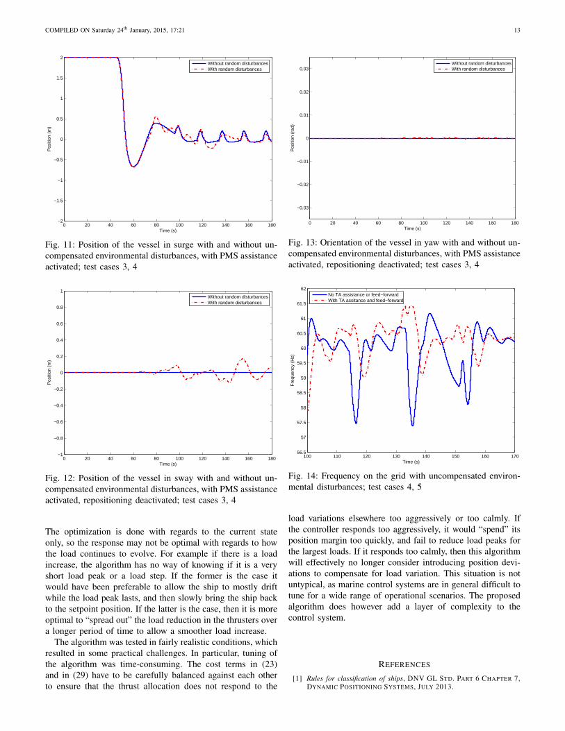
random component to the environmental force is the factthat the environmental forces are not deterministic in reality.The position of the vessel in surge with and without therandom environmental disturbances is shown in Figure 11.It shows that the disturbances due to the thrust allocationPMS assistance are not large compared to typical randomdisturbances. The effect of the thrust allocation algorithmmodification on the frequency is not qualitatively affected bythe random disturbances, as shown on Figure 14.

100 110 120 130 140 150 160 1700.5

0.55

0.6

0.65

0.7

0.75

0.8

0.85

0.9

0.95

1

Time (s)

Fra

ctio

n of

full

open


Fig. 9: Fuel injection rate on one of the generators; test cases1, 2, 3

0 20 40 60 80 100 120 140 160 180−2

−1.5

−1

−0.5

0

0.5

1

1.5

2

Pos

ition

(m

)

Time (s)


Fig. 10: Position of the vessel in surge; test cases 1, 2, 3

VI. DISCUSSION AND CONCLUSION

The proposed thrust allocation algorithm has been demon-strated to reduce load variations on a marine power plant bymaking the thrusters produce counteracting load variations thatpartially cancel the load variations from the other consumers.This can be taken advantage of either through reducing fre-quency variations as has been demonstrated in simulation, oralternatively by reducing the variations in the fuel index, thusreducing wear-and-tear on the engine, emissions and sooting.


0 20 40 60 80 100 120 140 160 180−2

−1.5

−1

−0.5

0

0.5

1

1.5

2

Pos

ition

(m

)

Time (s)

Without random disturbancesWith random disturbances

Fig. 11: Position of the vessel in surge with and without un-compensated environmental disturbances, with PMS assistanceactivated; test cases 3, 4

0 20 40 60 80 100 120 140 160 180−1

−0.8

−0.6

−0.4

−0.2

0

0.2

0.4

0.6

0.8

1

Pos

ition

(m

)

Time (s)


Fig. 12: Position of the vessel in sway with and without un-compensated environmental disturbances, with PMS assistanceactivated, repositioning deactivated; test cases 3, 4

The optimization is done with regards to the current stateonly, so the response may not be optimal with regards to howthe load continues to evolve. For example if there is a loadincrease, the algorithm has no way of knowing if it is a veryshort load peak or a load step. If the former is the case itwould have been preferable to allow the ship to mostly driftwhile the load peak lasts, and then slowly bring the ship backto the setpoint position. If the latter is the case, then it is moreoptimal to “spread out” the load reduction in the thrusters overa longer period of time to allow a smoother load increase.

The algorithm was tested in fairly realistic conditions, whichresulted in some practical challenges. In particular, tuning ofthe algorithm was time-consuming. The cost terms in (23)and in (29) have to be carefully balanced against each otherto ensure that the thrust allocation does not respond to the

0 20 40 60 80 100 120 140 160 180

−0.03

−0.02

−0.01

0

0.01

0.02

0.03

Pos

ition

(ra

d)

Time (s)


Fig. 13: Orientation of the vessel in yaw with and without un-compensated environmental disturbances, with PMS assistanceactivated, repositioning deactivated; test cases 3, 4

100 110 120 130 140 150 160 17056.5

57

57.5

58

58.5

59

59.5

60

60.5

61

61.5

62

Time (s)

Fre

quen

cy (

Hz)

No TA assistance or feed−forwardWith TA assitance and feed−forward

Fig. 14: Frequency on the grid with uncompensated environ-mental disturbances; test cases 4, 5

load variations elsewhere too aggressively or too calmly. Ifthe controller responds too aggressively, it would “spend” itsposition margin too quickly, and fail to reduce load peaks forthe largest loads. If it responds too calmly, then this algorithmwill effectively no longer consider introducing position devi-ations to compensate for load variation. This situation is notuntypical, as marine control systems are in general difficult totune for a wide range of operational scenarios. The proposedalgorithm does however add a layer of complexity to thecontrol system.

REFERENCES

[1] Rules for classification of ships, DNV GL STD. PART 6 CHAPTER 7,DYNAMIC POSITIONING SYSTEMS, JULY 2013.


100 110 120 130 140 150 160 170−5

0

5

10

15

20x 10

−3

Time (s)

For

ce/m

omen

t (p.

u.)

xyψ

Fig. 15: Environmental disturbances, including random un-compensated disturbances; test case 4 (test case 5 is quali-tatively similar but driven by a different random noise realiza-tion)

100 110 120 130 140 150 160 170−0.1

0

0.1

0.2

0.3

0.4

0.5

0.6

Time (s)

Pos

ition

dev

iatio

n (m

)

Actual positionDeviation estimate

Fig. 16: Position deviation estimate in surge due to effectsof the thrust allocation deviations, superpositioned on theactual position shows the interaction between the dynamicpositioning algorithm and the deviation in thrust allocation;test case 3

[2] A. K. ÅDNANES, “MARITIME ELECTRICAL INSTALLATIONS ANDDIESEL ELECTRIC PROPULSION,” ABB AS, TECH. REP., 2003.

[3] P. LAKSHMINARAYANAN AND Y. V. AGHAV, Modeling Diesel Com-bustion, F. F. LING, ED. SPRINGER, 2009.

[4] P. ECKERT AND S. RAKOWSKI, Combustion Engines Development.SPRINGER-VERLAG, 2012, CH. POLLUTANT FORMATION.

[5] C. D. RAKOPOULOS AND E. G. GIAKOUMIS, Diesel Engine TransientOperation. SPRINGER, 2009.

[6] T. A. JOHANSEN, T. P. FUGLSETH, P. TØNDEL, AND T. I. FOS-SEN, “OPTIMAL CONSTRAINED CONTROL ALLOCATION IN MARINESURFACE VESSELS WITH RUDDERS,” Control Engineering Practice,VOL. 16, NO. 4, PP. 457 – 464, 2008.

[7] N. A. JENSSEN AND B. REALFSEN, “POWER OPTIMAL THRUST ALLO-CATION,” IN MTS Dynamic Positioning Conference, HOUSTON, 2006.

[8] T. A. JOHANSEN, T. I. FOSSEN, AND S. P. BERGE, “CONSTRAINEDNONLINEAR CONTROL ALLOCATION WITH SINGULARITY AVOIDANCEUSING SEQUENTIAL QUADRATIC PROGRAMMING,” IEEE Trans. Con-trol Systems Technology, VOL. 12, PP. 211–216, 2004.

[9] T. A. JOHANSEN, T. I. BØ, E. MATHIESEN, A. VEKSLER, ANDA. SØRENSEN, “DYNAMIC POSITIONING SYSTEM AS DYNAMIC EN-ERGY STORAGE ON DIESEL-ELECTRIC SHIPS,” IEEE Transactions onPower Systems, 2014, (IN PRESS).

[10] D. RADAN, A. J. SØRENSEN, A. K. ÅDNANES, AND T. A. JOHANSEN,“REDUCING POWER LOAD FLUCTUATIONS ON SHIPS USING POWERREDISTRIBUTION CONTROL,” SNAME Journal of Marine Technology,VOL. 45, PP. 162–174, 2008.

[11] E. MATHIESEN, B. REALFSEN, AND M. BREIVIK, “METHODS FORREDUCING FREQUENCY AND VOLTAGE VARIATIONS ON DP VES-SELS,” IN MTS Dynamic Positioning Conference, HOUSTON, OCTOBER2012.

[12] T. A. JOHANSEN AND T. I. FOSSEN, “CONTROL ALLOCATION – ASURVEY,” Automatica, VOL. 49, NO. 5, PP. 1087 – 1103, 2013.

[13] A. VEKSLER, T. A. JOHANSEN, AND R. SKJETNE, “THRUST ALLO-CATION WITH POWER MANAGEMENT FUNCTIONALITY ON DYNAM-ICALLY POSITIONED VESSELS,” IN Proc. American Control Conf.,2012.

[14] ——, “TRANSIENT POWER CONTROL IN DYNAMIC POSITIONING-GOVERNOR FEEDFORWARD AND DYNAMIC THRUST ALLOCATION,” IN9th IFAC Conference on Manoeuvring and Control of Marine Craft,2012.

[15] L. PIVANO, T. A. JOHANSEN, AND . N. SMOGELI, “A FOUR-QUADRANT THRUST ESTIMATION SCHEME FOR MARINE PRO-PELLERS: THEORY AND EXPERIMENTS,” A Four-Quadrant ThrustController for Marine Propellers with Loss Estimation and Anti-Spin:Theory and Experiments, VOL. 17, PP. 215–226, 2009.

[16] P. MACIEL, A. KOOP, AND G. VAZ, “MODELLING THRUSTER-HULLINTERACTION WITH CFD,” IN 32nd International Conference on Ocean,Offshore and Arctic Engineering, Nantes, France., JUNE 2013.

[17] T. I. FOSSEN, Handbook of Marine Craft Hydrodynamics and MotionControl, APRIL 2011.

[18] ——, Marine Control Systems. TAPIR TRYKKERI, 2002.[19] O. M. FALTINSEN, Hydrodynamics of High-Speed Marine Vehicles.

CAMBRIDGE UNIVERSITY PRESS, 2006.[20] C. HOLDEN, “MODELLING AND CONTROL OF PARAMETRIC ROLL

RESONANCE,” PH.D. DISSERTATION, NTNU, JUNE 2011.[21] Nomenclature for Treating the Motion of a Submerged Body Through

a Fluid, TECHNICAL AND RESEARCH BULLETIN NO. 1-5, THE SOCI-ETY OF NAVAL ARCHITECTS AND MARINE ENGINEERS, TECHNICALAND RESEARCH COMMITTEE STD., 1950.

[22] D. RADAN, “INTEGRATED CONTROL OF MARINE ELECTRICAL POWERSYSTEMS,” PH.D. DISSERTATION, NTNU, 2008.

[23] D. RADAN, T. A. JOHANSEN, A. J. SØRENSEN, AND A. K. ÅDNANES,“OPTIMIZATION OF LOAD DEPENDENT START TABLES IN MARINEPOWER MANAGEMENT SYSTEMS WITH BLACKOUT PREVENTION,”WSEAS Trans. Circuits and Systems, VOL. 4, 2005.

[24] T. I. BØ AND T. A. JOHANSEN, “SCENARIO BASED FAULT TOLER-ANT MODEL PREDICTIVE CONTROL FOR DIESEL-ELECTRIC MARINEPOWER PLANT,” IN Proc. MTS/IEEE OCEANS, 2013.

[25] S. SAVOY, “ENSCO 7500 POWER MANAGEMENT SYSTEM DESIGN,FUNCTIONALITY AND TESTING,” IN MTS Dynamic Positioning Con-ference, 2002.

[26] X. SHI, Y. WEI, J. NING, M. FU, AND D. ZHAO, “OPTIMIZING ADAP-TIVE THRUST ALLOCATION BASED ON GROUP BIASING METHOD FORSHIP DYNAMIC POSITIONING,” IN Proceeding of the IEEE InternationalConference on Automation and Logistics, Chongqing, China, 2011.

[27] N. XIROS, Robust Control of Diesel Ship Propulsion. SPRINGER-VERLAG, 2002.

[28] G. THEOTOKATOS, “A COMPARATIVE STUDY ON MEAN VALUE MOD-ELLING OF TWO-STROKE MARINE DIESEL ENGINE,” IN Proceedings ofthe 2nd International Conference on Maritime and Naval Science andEngineering. WORLD SCIENTIFIC AND ENGINEERING ACADEMYAND SOCIETY, 2009, PP. 107–112.

[29] ——, “SHIP PROPULSION PLANT TRANSIENT RESPONSE INVESTIGA-TION USING A MEAN VALUE ENGINE MODEL,” International JournalOf Energy, VOL. 2, NO. 4, PP. 66–74, 2008.

[30] R. SKJETNE, “MODELING A DIESEL-GENERATOR POWER PLANT,”LECTURE NOTES IN COURSE TMR4290, 2011, NTNU, OCTOBER2011.

[31] I. BOLDEA, Synchronous Generators. CRC PRESS, NOVEMBER2005.


[32] S. ROY, O. MALIK, AND G. HOPE, “ADAPTIVE CONTROL OF SPEEDAND EQUIVALENCE RATIO DYNAMICS OF A DIESEL DRIVEN POWER-PLANT,” IEEE Transactions on Energy Conversion, VOL. 8, NO. 1, PP.13 –19, MAR 1993.

[33] A. VEKSLER, T. A. JOHANSEN, E. MATHIESEN, AND R. SKJETNE,“GOVERNOR PRINCIPLE FOR INCREASED SAFETY AND ECONOMY ONVESSELS WITH DIESEL-ELECTRIC PROPULSION,” IN Proc. EuropeanControl Conf., 2013.

[34] T. I. BØ, “DYNAMIC MODEL PREDICTIVE CONTROL FOR LOAD SHAR-ING IN ELECTRIC POWER PLANTS FOR SHIPS,” MASTER’S THESIS,NTNU, 2012.

[35] Governing Fundamentals and Power Management, 2620TH ED.,WOODWARD, 2004.

[36] TCA - The Benchmark, MAN DIESEL & TURBO, 86224 AUGSBURG,GERMANY, 2013.

APPENDIX AMODELING OF THE DIESEL PRIME MOVER

The intended area of application for this marine dieselengine model is in design and testing of control systems formarine power plants. It is intended to be general enoughto be easily configurable, but still describe the engine bothunder relatively low load variations that are expected duringnormal operations, and during extreme load variations whenthe engine would be asked to deliver as much power as it isphysically able.

A. Assumptions and simplifications

Compared to the model in [27], the following assumptionsand simplifications are made in this model:

• The angular velocity of the turbine is assumed to dependon the generated power only. In reality this relationship isquite dynamic, with other factors such as thermodynamicrelationships incorporated in the exhaust manifold. Still,both generated power and the exhaust volume that drivesthe turbocharger depend upon how much fuel is burnedper unit of time, and both relationships are linear to somedegree.

• To calculate the Air-to-Fuel ratio (AF) after each injec-tion, it is assumed that the fuel injected into the cylinderin each cycle is proportional to the fuel index position.The amount of air entering the cylinder is assumed tobe linearly dependent on the velocity of the turbochargercompressor. If the compressor velocity is zero, then theamount of air entering will be ma,0, and it will linearlyincrease to a maximum value as the velocity of thecompressor approaches its maximum value.

• There is a delay in the order of (60/N) · (2/zc) secondsfrom fuel index change until the corresponding changeof torque on the drive shaft. The main cause of the delayis that it takes time before the new measure of fuel isinjected into the next cylinder in the firing sequence, andin addition it takes some more time before the ignitionleads to increased in-cylinder pressure and then increasedtorque on the drive shaft [5, p. 25]. The nominal RPMof the engines in the simulation was around N = 1800,so this delay had little practical consequence and wasignored.

• On older engines, setting a new value for the fuel indexinvolved moving an actual fuel rack, a mechanical devicewhich determined the fuel injection rate into the engine,

resulting in a certain amount of lag. On newer engineswith direct fuel injection there is no physical fuel rack,so this delay is not included in the model.

• Performance of a diesel engine during a large transientis limited by the performance of the turbocharger, whichneeds time to increase the pressure in the intake man-ifold. Until it does, the concentration of oxygen in thecombustion chamber will limit the combustion.

• The damping due to friction is mostly a function of thecurrent engine RPM. Since the engine in a power plantnormally operates in a narrow RPM range, this frictionis not important for the dynamical performance of theengine and was not modeled.

B. Variables

The variables used for the diesel engine model are describedin Table VI.

Symbol Descriptionpe Break mean effective pressure in the cylinders (p.u.)tm Total mechanical torque from an engine (p.u.)te Electrical torque (p.u.)pe,r Rated BMEP (Pa)N Instantaneous crank shaft RPMNr Nominal engine RPMzc Number of cylindersVh Cylinder volume (m3)ηc Combustion efficiency (non-dimensional, p.u.)Fr Fuel rack/fuel index position (nondimensional, p.u.), which

determines the amount of fuel injected into the combustioncylinders per diesel cycle.

ωt Turbocharger rotational velocity (p.u.)Tt Turbocharger dynamics time constantma,0 Air flow (mass) without the turbocharger as fraction of the

maximal airflowAFn Nominal air-to-fuel ratio on max turbocharger velocity and

max BMEPAFlow Air-to-fuel ratio at which the combustion stops due to

excessive in-cylinder cooling from the injected fuel.AFhigh Air-to-fuel ratio at which full combustion is achieved.

Typical values: 20-27 for HFO, 17-20 for Diesel OilP Current engine power output (Watt)Pl Power consumed by the load (Watt)Pr Rated engine power (Watt)I Moment of inertia of the rotating mass in the genset

(kg ·m2)H Inertia constant of the engine, represented as the time needed

for the engine running at nominal power to produce theenergy equivalent to the kinetic energy in the rotating mass

at nominal speed.

TABLE VI: Variables used for the diesel engine model.

C. Formulas

AF =ma,0 + (1−ma,0)ωt

Fr·AFn (36)

ηc =

1 AF ≥ AFhighAF−AFlow

AFhigh−AFlowAFlow < AF < AFhigh

0 AF ≤ AFlow(37)

tm = pe = ηcFr (38)


ωt = −1/Tt(ωt − pe) (39)

P = pe,rpezcVhN/60 = PrtmN/Nr (40)

H =12I(

2πNr

60

)2Pr

(41)

N =12Nr(tm − te)

H(42)

The torque balance enters the swing equation in (42); theelectrical torque te is an external input to this model andhas to come from the model of the generator. The equation(39) is a rough representation of the turbocharger lag, whichincludes a large variation of effects, such as pressure buildupin the exhaust manifold (if the turbo is not pulse charged),acceleration of the turbocharger shaft and buildup of thepressure in the intake manifold, as well as heating up theengine to the new working temperature.

The fuel rack can change the fuel injection arbitrarily, whichroughly translates to a change in BMEP (pe in per-unit) aftera short injection and combustion delay which may not bemodeled. Since cycle-mean torque delivery is proportional toBMEP, the per-unit torque tm has the same numerical value,as expressed in (38). If the turbocharger didn’t have time toincrease air delivery sufficiently, then either the combustionefficiency will be reduced as per (38), or the fuel rack limiterwill be activated and not allow the fuel rack to exceed themaximal efficient value.

D. Numerical values

The parameters for the simulation are matched so that theyrepresent a typical marine diesel engine of the size mentionedin section V-C. The stoichiometric ratios AF∗ are takenwithin the range specified in [27, page 23], AFhigh = 20,AFlow = 14. The air-to-fuel ratio under full power and fullydeveloped turbocharger velocity is set to 27. The naturallyperspired efficiency ma0 is set to 0.2 to reflect the compressionratio in the modern marine turbochargers, which is around5 [36]. The losses in the conversion of power from themechanical to electrical systems are not modeled, so the ratedpower Pr of each diesel engine can be calculated from thegenset rated power as mentioned in section V-C.

APPENDIX B

ACKNOWLEDGMENTS

This work is partly sponsored by the Research Council ofNorway by the KMB project D2V, project number 210670,and through the Centres of Excellence funding scheme, projectnumber 223254 – AMOS. Eirik Mathiesen is employed withKongsberg Maritime. Valuable comments that led to significantimprovements of parts of the paper were contributed by TrondToftevaag of SINTEF, Eilif Pedersen of NTNU, and BjørnarRealfsen of Kongsberg.

Aleksander Veksler is a graduate student at theInstitute of Engineering Cybernetics at the Norwe-gian University of Science and Technology (NTNU),Trondheim. He was born in 1982 and receivedhis MSc in Engineering Cybernetics in 2009 fromNTNU. He was a research visitor to UCSD in2008/2009 while working on his Master’s thesis.

Professor Tor A. Johansen was born in 1966,received his MSc degree in 1989 and Ph.D. degreein 1994, both in electrical and computer engineeringfrom the Norwegian University of Science and Tech-nology, Trondheim. He worked at SINTEF Elec-tronics and Cybernetics as a researcher before hewas appointed Associated Professor in EngineeringCybernetics at the Norwegian University of Scienceand Technology in Trondheim in 1997 and waspromoted Professor in 2001. He was a researchvisitor at the USC, TU-Delft and UCSD. He has

published more than 100 articles in international journals as well as numerousconference articles and book chapters in the areas of nonlinear control andestimation, optimization, adaptive control, and MPC with applications inthe marine, automotive, biomedical and process industries. He has beensupervising more than 10 PhD students, holds several patents, and has beendirecting numerous research projects. In December 2002 Johansen co-foundedthe company Marine Cybernetics AS where he was Vice President until 2008.Prof. Johansen received the 2006 Arch T. Colwell Merit Award of the SAE,and is currently a principal researcher within the Center of Excellence onAutonomous Marine Operations and Systems (AMOS).

Professor Roger Skjetne received in 2000 his MScdegree in control engineering at UCSB and hisPhD degree in 2005 at NTNU, for which he wasawarded the Exxon Mobil prize for best PhD thesisin applied research. Prior to his studies, he workedas an electrician for Aker Elektro AS on numerousoil installations for the North Sea. In 2004-2009,he was employed in Marine Cybernetics AS whichoffered services for independent verification by HILsimulation on safety-critical marine control systems.From August 2009 he has held the position of

Professor in Marine Control Engineering at the Dept. of Marine Technologyat NTNU. His research interests are within Arctic Dynamic Positioning andIce Management systems for ships and rigs, environmentally robust controlof electric power systems on ships and rigs, and nonlinear control theoryfor motion control of single and groups of marine vessels. Roger Skjetne isproject manager for the Arctic DP research project, and associated researcherin the CoE Centre for Ships and Ocean Structures (CeSOS), CRI SustainableArctic Marine and Coastal Technology (SAMCoT), and CoE AutonomousMarine Operations and Systems (AMOS).

Eirik Mathiesen Eirik Mathiesen is a principalengineer at Kongsberg Maritime, responsible forapplication development of power management anddynamic positioning integration. He graduated fromVestfold University College and entered the RoyalNorwegian Navy as an electrical supervisor in 1996.He joined Kongsberg Maritime in 1997 as a projectengineer and has been involved with power man-agement design for drillships and semi-submersiblevessels on more than 50 instalations. Mathiesen is aco-holder of two patents on dynamic load prediction

and dynamic load compensation.

thrust allocation with dynamic power consumption

Documents