logo

Threshold Accepting for Credit RiskAssessment and Validation

M. Lyra1 A. Onwunta P. Winker

COMPSTAT 2010

August 24, 2010

1Financial support from the EU Commission through COMISEF isgratefully acknowledged

logo

Introduction Ex-post validation Optimal buckets Conclusion Appendix

1 IntroductionBasel II and credit risk clusteringOptimal size and number of clusters

2 Ex-post validationActual number of defaults

3 Optimal buckets

4 ConclusionSummary - OutlookFor further reading

logo

Introduction Ex-post validation Optimal buckets Conclusion Appendix

1 IntroductionBasel II and credit risk clusteringOptimal size and number of clusters

2 Ex-post validationActual number of defaults

3 Optimal buckets

4 ConclusionSummary - OutlookFor further reading

logo

Introduction Ex-post validation Optimal buckets Conclusion Appendix

Basel II and credit risk clustering

logo

Introduction Ex-post validation Optimal buckets Conclusion Appendix

Basel II and credit risk clustering

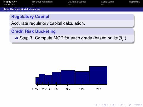
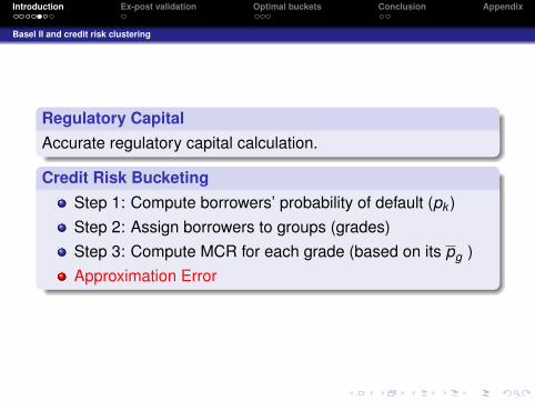
Regulatory CapitalAccurate regulatory capital calculation.

Credit Risk BucketingStep 1: Compute borrowers’ probability of default (pk )

logo

Introduction Ex-post validation Optimal buckets Conclusion Appendix

Basel II and credit risk clustering

Regulatory CapitalAccurate regulatory capital calculation.

Credit Risk BucketingStep 1: Compute borrowers’ probability of default (pk )

logo

Introduction Ex-post validation Optimal buckets Conclusion Appendix

Basel II and credit risk clustering

Regulatory CapitalAccurate regulatory capital calculation.

Credit Risk BucketingStep 2: Assign borrowers to groups (grades)

logo

Introduction Ex-post validation Optimal buckets Conclusion Appendix

Basel II and credit risk clustering

Regulatory CapitalAccurate regulatory capital calculation.

Credit Risk BucketingStep 3: Compute MCR for each grade (based on its pg )

logo

Introduction Ex-post validation Optimal buckets Conclusion Appendix

Basel II and credit risk clustering

Regulatory CapitalAccurate regulatory capital calculation.

Credit Risk BucketingStep 1: Compute borrowers’ probability of default (pk )Step 2: Assign borrowers to groups (grades)Step 3: Compute MCR for each grade (based on its pg )Approximation Error

logo

Introduction Ex-post validation Optimal buckets Conclusion Appendix

Basel II and credit risk clustering

Approximation ErrorUsing pg instead of individual pkcauses a loss in precision.

Meaningful assignment of borrowers to clustersChoose appropriate size and number of clusters to minimizeover/understatement of MCR and allow statistical ex-postvalidation

logo

Introduction Ex-post validation Optimal buckets Conclusion Appendix

Optimal size and number of clusters

Optimal Credit Risk Rating SystemChoose appropriate size and number of grades

(ex post )Predicts defaults correctly

logo

Introduction Ex-post validation Optimal buckets Conclusion Appendix

Optimal size and number of clusters

Optimal Credit Risk Rating SystemChoose appropriate size and number of grades

(ex post )Predicts defaults correctly

logo

Introduction Ex-post validation Optimal buckets Conclusion Appendix

Optimal size and number of clusters

Optimal Credit Risk Rating SystemChoose appropriate size and number of grades

(ex post )Predicts defaults correctly

logo

Introduction Ex-post validation Optimal buckets Conclusion Appendix

1 IntroductionBasel II and credit risk clusteringOptimal size and number of clusters

2 Ex-post validationActual number of defaults

3 Optimal buckets

4 ConclusionSummary - OutlookFor further reading

logo

Introduction Ex-post validation Optimal buckets Conclusion Appendix

Actual number of defaults

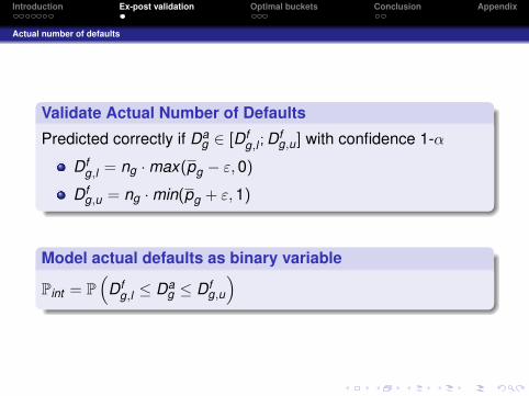
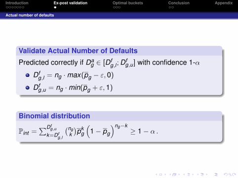
Validate Actual Number of Defaults

Predicted correctly if Dag ∈ [Df

g,l ; Dfg,u] with confidence 1-α

Dfg,l = ng ·max(pg − ε, 0)

Dfg,u = ng ·min(pg + ε, 1)

logo

Introduction Ex-post validation Optimal buckets Conclusion Appendix

Actual number of defaults

Validate Actual Number of Defaults

Predicted correctly if Dag ∈ [Df

g,l ; Dfg,u] with confidence 1-α

Dfg,l = ng ·max(pg − ε, 0)

Dfg,u = ng ·min(pg + ε, 1)

Model actual defaults as binary variable

Pint = P(

Dfg,l ≤ Da

g ≤ Dfg,u

)

logo

Introduction Ex-post validation Optimal buckets Conclusion Appendix

Actual number of defaults

Validate Actual Number of Defaults

Predicted correctly if Dag ∈ [Df

g,l ; Dfg,u] with confidence 1-α

Dfg,l = ng ·max(pg − ε, 0)

Dfg,u = ng ·min(pg + ε, 1)

Binomial distribution

Pint =∑Df

g,u

k=Dfg,l

(ngk

)pk

g

(1− pg

)ng−k≥ 1− α .

logo

Introduction Ex-post validation Optimal buckets Conclusion Appendix

1 IntroductionBasel II and credit risk clusteringOptimal size and number of clusters

2 Ex-post validationActual number of defaults

3 Optimal buckets

4 ConclusionSummary - OutlookFor further reading

logo

Introduction Ex-post validation Optimal buckets Conclusion Appendix

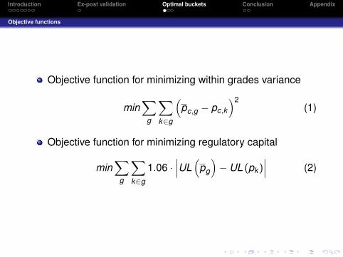
Objective functions

Objective function for minimizing within grades variance

min∑

g

∑k∈g

(pc,g − pc,k

)2(1)

Objective function for minimizing regulatory capital

min∑

g

∑k∈g

1.06 ·∣∣∣UL

(pg

)− UL (pk )

∣∣∣ (2)

logo

Introduction Ex-post validation Optimal buckets Conclusion Appendix

Feasible region

Feasible regionMinimizing regulatory capital using the validation technique(α = 1.5%, ε = 1% )

0 0.05 0.1 0.15

0.005

0.01

0.015

0.02

0.025

0.03

α

ε

g = 7g = 11g = 13

logo

Introduction Ex-post validation Optimal buckets Conclusion Appendix

Empirical Findings

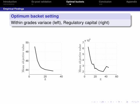
Optimum backet settingWithin grades variace (left), Regulatory capital (right)

0 20 40

44

46

48

50

g

Mea

nobje

ctiv

evalu

e

0 20 40 60

2

3

4

5

6

7x 106

gM

ean

obje

ctiv

evalu

e

Figure:

logo

Introduction Ex-post validation Optimal buckets Conclusion Appendix

1 IntroductionBasel II and credit risk clusteringOptimal size and number of clusters

2 Ex-post validationActual number of defaults

3 Optimal buckets

4 ConclusionSummary - OutlookFor further reading

logo

Introduction Ex-post validation Optimal buckets Conclusion Appendix

Summary - Outlook

SummaryMinimum capital requirements to cover unexpected lossesThreshold Accepting to cluster loans with real-worldconstraintsOptimal size and number of buckets based on ex-postvalidation

OutlookRelax default risk independence constraintAlternative assumptions for actual default distributions

logo

Introduction Ex-post validation Optimal buckets Conclusion Appendix

For further reading

P. Winker.Onptimization Heuristics in Econometrics: Applications ofThreshold Accepting.Wiley, New York, 2001.

Basel Committee on Banking Supervision.Capital Standards a Revised Framework.Bank for International Settlements, 2006.

M. Lyra and J. Paha and S. Paterlini and P. Winker.Optimization Heuristics for Determining Internal RatingGrading Scales.Computational Statistics & Data Analysis, Article in Press.

M. Kalkbrener and A. Onwunta.Validation Structural Credit Portfolio Models.In:Model Risk in Finance, forthcoming.

logo

Introduction Ex-post validation Optimal buckets Conclusion Appendix

For further reading

P. Winker.Onptimization Heuristics in Econometrics: Applications ofThreshold Accepting.Wiley, New York, 2001.

Basel Committee on Banking Supervision.Capital Standards a Revised Framework.Bank for International Settlements, 2006.

M. Lyra and J. Paha and S. Paterlini and P. Winker.Optimization Heuristics for Determining Internal RatingGrading Scales.Computational Statistics & Data Analysis, Article in Press.

M. Kalkbrener and A. Onwunta.Validation Structural Credit Portfolio Models.In:Model Risk in Finance, forthcoming.

logo

Introduction Ex-post validation Optimal buckets Conclusion Appendix

For further reading

P. Winker.Onptimization Heuristics in Econometrics: Applications ofThreshold Accepting.Wiley, New York, 2001.

Basel Committee on Banking Supervision.Capital Standards a Revised Framework.Bank for International Settlements, 2006.

M. Lyra and J. Paha and S. Paterlini and P. Winker.Optimization Heuristics for Determining Internal RatingGrading Scales.Computational Statistics & Data Analysis, Article in Press.

M. Kalkbrener and A. Onwunta.Validation Structural Credit Portfolio Models.In:Model Risk in Finance, forthcoming.

logo

Introduction Ex-post validation Optimal buckets Conclusion Appendix

For further reading

P. Winker.Onptimization Heuristics in Econometrics: Applications ofThreshold Accepting.Wiley, New York, 2001.

Basel Committee on Banking Supervision.Capital Standards a Revised Framework.Bank for International Settlements, 2006.

M. Lyra and J. Paha and S. Paterlini and P. Winker.Optimization Heuristics for Determining Internal RatingGrading Scales.Computational Statistics & Data Analysis, Article in Press.

M. Kalkbrener and A. Onwunta.Validation Structural Credit Portfolio Models.In:Model Risk in Finance, forthcoming.

logo

Introduction Ex-post validation Optimal buckets Conclusion Appendix

Data descriptionportfolio of 93 580retail borrowers.LGDs range between0.17 and 1.

pk vary from0.000001% to 30%.

0 0.05 0.1 0.15 0.2 0.25 0.3 0.350

0.5

1

1.5

2

2.5

3

3.5

4x 10

4

Probabilities of default

Fre

quen

cy

logo

Introduction Ex-post validation Optimal buckets Conclusion Appendix

Credit Risk Assignment - Side Constraints

Enforced by constraint handling techniquespg in bucket � 0.03%

Each bucket � 35% of total bank exposureConsidered in the structure of the algorithm

No bucket overlappingBuckets correspond to all borrowers

logo

Introduction Ex-post validation Optimal buckets Conclusion Appendix

Optimization HeuristicsOptimal partition of k bank clients in gclusters

1 Generate random startingthresholds (candidate solution)

2 Alter current candidate solution3 Accept or reject new candidate

solution4 Repeat until a very good solution

is found

logo

Introduction Ex-post validation Optimal buckets Conclusion Appendix

Optimization HeuristicsOptimal partition of k bank clients in gclusters

1 Generate random startingthresholds (candidate solution)

2 Alter current candidate solution3 Accept or reject new candidate

solution4 Repeat until a very good solution

is found

logo

Introduction Ex-post validation Optimal buckets Conclusion Appendix

Optimization HeuristicsOptimal partition of k bank clients in gclusters

1 Generate random startingthresholds (candidate solution)

2 Alter current candidate solution3 Accept or reject new candidate

solution4 Repeat until a very good solution

is found

logo

Introduction Ex-post validation Optimal buckets Conclusion Appendix

Optimization HeuristicsOptimal partition of k bank clients in gclusters

1 Generate random startingthresholds (candidate solution)

2 Alter current candidate solution3 Accept or reject new candidate

solution4 Repeat until a very good solution

is found

logo

Introduction Ex-post validation Optimal buckets Conclusion Appendix

Threshold Accepting - The Basic Idea

Generate a random candidate solution and determine itsobjective function valueRepeat a predefined number of iterations

Modify candidate solution and determine its objectivefunction valueReplace current solution with modified solution if newsolutions yields

An improved objective function value orA deterioration that is smaller than some threshold(predefined by a threshold sequence)

logo

Introduction Ex-post validation Optimal buckets Conclusion Appendix

Algorithm 1 Threshold Accepting Algorithm.1: Initialize nR , nSτ , and τr , r = 1, 2,. . . ,nR

2: Generate at random a solution x0 ∈ [αlαu]× [βlβu]3: for r = 1 to nR do4: for i = 1 to nSτ do5: Generate neighbor at random, x1 ∈ N (x0)6: if f (x1)− f (x0) < τr then7: x0 = x1

8: end if9: end for

10: end for

logo

Introduction Ex-post validation Optimal buckets Conclusion Appendix

Threshold Accepting - Candidate Solutions

Starting Candidate SolutionFor g buckets, select g-1 upper bucket thresholds fromactual pdsDiscrete search ⇒ Each solution constitutes a new partition

New Candidate SolutionDetermine some bucket threshold of current solutionrandomlyReplace with new pd from interval [next lower threshold;next higher threshold]Shrink interval linearly in the number of iterations;[(I + 1)− i]/I

logo

Introduction Ex-post validation Optimal buckets Conclusion Appendix

Threshold Accepting - Updating Objective Function Values

Alter only one bucket threshold per iterationNew objective function differs from that of the currentsolution only in contribution of two bucketsOnly compute those two buckets’ fitness and updateobjective function value of current solutionConsequence: Tremendous increase in search speed

logo

Introduction Ex-post validation Optimal buckets Conclusion Appendix

Threshold Accepting - Threshold Sequence

Idea: Use mean of last 100 weighted fitness differences (inabsolute values) as threshold TIf last fitness differences were mainly

improvements, T shrinks ⇒ Stay on path to (local) optimumdeteriorations, T increases ⇒ Overcome (local) optimumand search for a new one

Weights (w1, w2) for restrictive threshold sequenceFitness improvement (frequent and high at the beginning ofthe search) ⇒ w1 = i/IFitness deterioration (frequent and high at the end of thesearch) ⇒ w2 = 1− i/I

Scale above means with (1-i/I) for further restrictiveness

logo

Introduction Ex-post validation Optimal buckets Conclusion Appendix

Algorithm 2 Pseudocode for TA with data driven generation ofthreshold sequence.

1: Initialize I, Ls = (0, . . . , 0) of length 1002: Generate at random an initial solution xc , set τ = f (xc)3: for i = 1 to I do4: Generate at random xn ∈ N (xc)5: Delete first element of Ls6: if f (xn)− f (xc) < 0 then7: add |f (xn)− f (xc)| · (i/I) as last element to Ls8: else9: add |f (xn)− f (xc)| · (1− i/I) as last element to Ls

10: end if11: τ = Ls · (1− i/I)12: if f (xn)− f (xc) < τ then13: xc = xn

14: end if15: end for

logo

Introduction Ex-post validation Optimal buckets Conclusion Appendix

Constraint Handling - Rejection Technique in TA

Both candidate solutions are feasibleTA: Select the new candidate if f (gn) + T ≤ f (gc)

One solution is feasible, select the feasibleNo feasible solution

Select fewer violationsSelect with regard to fitness

TA: Select the new candidate if f (gn) + T ≤ f (gc)

logo

Introduction Ex-post validation Optimal buckets Conclusion Appendix

Constraint Handling - Penalty Technique in TA

Penalize candidate solutions’ objective value by a factorA ∈ [1; 3.7183] ⇒ fc(g) = fu(g) · AA rises in the number of iterations i and the degree of

constraint violation a ∈ [0; 1] ⇒ A =(

1 + exp( iI )

)a

a = 1, ifall buckets besides one are empty, andEAD is concentrated in one bucket.

Select the new candidate if fc(gn) + T ≤ fc(gc)

logo

Introduction Ex-post validation Optimal buckets Conclusion Appendix

Table: Objective function for minimizing within grades variance(1)

Best Mean Worst s.d. q90% Freqg = 7

TAa 18.6836 18.6836 18.6836 3.6731 · 10−8 18.6836 8/10TAb 18.6552 24.4809 46.2984 8.2478 24.8221 1/10

g = 10TAa 9.7293 9.7293 9.7293 5.3490 · 10−7 9.7293 1/10TAb 9.1118 10.3545 10.9233 0.8520 10.9108 1/10

g = 13TAa 6.6716 6.6716 6.6716 2.9353 · 10−6 6.6716 1/10TAb 6.5974 10.0515 14.5469 2.7151 12.4890 1/6

g = 16TAa 5.2454 5.2454 5.2454 1.9032 · 10−6 5.2454 1/10TAb 10.3647 10.3647 10.3647 0.0000 10.3647 1/1

aActual number of defaults constraintbUnexpected loss constraint

logo

Introduction Ex-post validation Optimal buckets Conclusion Appendix

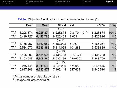
Table: Objective function for minimizing unexpected losses (2)

Best Mean Worst s.d. q90% Freqg = 7

TAa 6,228,874 6,228,874 6,228,874 9.8170 · 10−10 6,228,874 10/10TAb 6,419,727 6,423,788 6,426,403 2,053 6,420,826 1/10

g = 11TAa 4,165,257 4,167,952 4,182,902 5, 999 4,165,257 7/10TAb 5,534,072 5,636,388 5,814,094 101,283 5,538,839 1/10

g = 13TAa 3,425,092 3,435,627 3,436,798 3,701.71 3,436,798 1/10TAb 5,192,945 5,608,280 5,929,156 230,630 5,846,709 1/9

g = 15TAa 3,245,441 3,245,636 3,247,260 571.05 3,245,445 1/10TAb 5,627,306 6,285,472 7,166,148 647,632 6,945,510 1/3

aActual number of defaults constraintbUnexpected loss constraint