three-wave interaction solitons in optical parametric amplification
TRANSCRIPT

5815
PHYSICAL REVIEW E MAY 1999VOLUME 59, NUMBER 5
Three-wave interaction solitons in optical parametric amplification
E. Ibragimov* and A. A. Struthers†
Department of Mathematical Sciences, Michigan Technological University, Houghton, Michigan 49931-1295
D. J. Kaup‡
Institute of Nonlinear Studies and Department of Mathematics and Physics, Clarkson University, Potsdam, New York 13699-
J. D. KhaydarovContinuum Incorporated, Santa Clara, California 95091
K. D. SingerDepartment of Physics, Case Western Reserve University, Cleveland, Ohio 44106
~Received 1 July 1998; revised manuscript received 5 January 1999!
This paper applies three-wave interaction~TWI!-soliton theory to optical parametric amplification when thesignal, idler, and pump wave can all contain TWI solitons. We use an analogy between two different velocityregimes to compare the theory with output from an experimental synchronously pumped optical parametricamplifier. The theory explains the observed inability to compress the intermediate group-velocity wave and20-fold pulse compression in this experiment. The theory and supporting numerics show that one can effec-tively control the shape and energy of the optical pulses by shifting the TWI solitons in the pulses.@S1063-651X~99!16505-X#
PACS number~s!: 42.65.Tg, 42.65.Yj, 42.65.Re, 42.65.Ky
iha
thu
-
ssV
ron
inicagn
m
y
sn-st,r ao
ionp-nsg
notov-m
por-
ringingheasf
the
ing
putm-the
y in
rey,
I. INTRODUCTION
To adequately describe three-wave interactions~TWI’s!involving ultrashort laser pulses (t<10 ps), it is necessary toaccount for dispersive effects. Normally, such effects limconversion efficiency and elongate pulses in secondmonic generation~SHG!, sum frequency generation~SFG!,optical parametric generation~OPG!, and optical parametricamplification processes. However, as early as in 1968@1# itwas shown that in optical parametric amplification due togroup-velocity mismatch, the fundamental wave can be sstantially compressed in a degenerate interaction~when thegroup velocities of the two fundamentals are equal!. Morerecently it was predicted theoretically@2,3# and observed experimentally@4,5# that group-velocity mismatch~GVM! cancompress ultrashort laser pulses in SHG and SFG proceIn recent experiments pulse compression ascribed to Gwas also observed in OPG and OPA experiments@6–9#. Thatthis compression was soliton in nature, as originally pposed in Ref.@3#, had until very recently not been giveadequate consideration.
In Refs.@10,11# the soliton nature of pulse compressionthe presence of the GVM was explained using analytsoliton solutions@12,13# derived from the inverse scatterintransform~IST!: extensions of these soliton solutions to nozero phase mismatch were contained in@11#, where thesesolitons were termed TWI-solitons to distinguish them fro
*Electronic address: [email protected] Present addElectrical Engineering, University of Maryland, Baltimore CountBaltimore, MD 21250.
†Electronic address: [email protected]‡Electronic address: [email protected]
PRE 591063-651X/99/59~5!/6122~16!/$15.00
tr-
eb-
es.M
-
l
-
other more familiar solitons. TWI solitons, although theexist in quadraticx (2) media, differ greatly from the well-known solitary waves generated by cascadingx (2)3x (2)
processes@14,15#. Unlike the cascaded waves, TWI solitonare not a composition of two waves with different frequecies and oscillatory profiles moving together. In contraTWI solitons are single frequency pulses with smooth, fosingle TWI-soliton sech, profiles. Moreover, TWI solitons dnot require high second-order group-velocity dispers~GVD! and are supported entirely by the first-order grouvelocity mismatch effect. This feature makes TWI solitoespecially attractive for applications in all optical switchin@16#.
The underlying scattering problem~developed in Refs.@12,13#, and summarized in Ref.@17#! for the TWI system isthe unwieldy third order Zahkarov-Manakov~ZM! system ofdifferential equations. Fortunately, when the pulses dooverlap the ZM system factors into three simpler ZahkarShabat~ZS! scattering problems: the ZS scattering probleunderlies the nonlinear Schro¨dinger equation~NLS! solitontheory, and has been intensively studied because of imtant applications in optical data transmission.
The IST theory shows a connection between the scatteproblem for the NLS system and the asymptotic scatterproblems for the TWI system. A connection between tTWI system and NLS equation is not surprising. As early1976 the authors of@18# noted solitonlike propagation ooptical pulses in quadratic media. These phenomena aresubject of recent intense theoretical and experimental@14,15#investigation. The connection between the ZM scatterproblem and three ZS scattering problems~one for theasymptotic profile of each frequency! shows that we shouldexpect profiles similar to those seen in the NLS as outfrom the three-wave interaction. However, one must remeber that, although the inverse scattering problems aresame for the NLS and the asymptotics for each frequenc
ss:
6122 ©1999 The American Physical Society

s
oltrlau
tioe
olysss
nio
insa
co
thon-
almis-olta:ex
edli-ea
ne
edrtye-ithi-
veioschIn
,
andn
id
a
tter-
toithnnome
orearnotlem-ZM
en-
siss.
tonfZS
s-gnalwe
PRE 59 6123THREE-WAVE INTERACTION SOLITONS IN OPTICAL . . .
TWI, the temporal propagation equations are, of courcompletely different.
In this paper we present results obtained using IST todescribing pulse compression effects in optical parameamplification: it appears that IST theory provides an expnation of a substantial body of experimental data accumlated over the last few years in optical parametric generaand optical harmonic generation by ultrashort laser pulsSpecifically, we explain the experimentally measured 20-fcompression@6,7# of the idler wave in a synchronouslpumped optical parametric generator, and note the succeexplanation@19# of the compression reported in these work
II. BASIC PROPERTIES OF TWI SOLITONS
A numerical study in Ref.@11# shows that group velocitydispersion is negligible in most practical cases and weglect GVD effects. In this regime the three-wave interactis described by the following system of three equations:
]A1
]z1
1
v1
]A1
]t5A3A2 ,
]A2
]z1
1
v2
]A2
]t5A3A1 , ~1!
]A3
]z1
1
v3
]A3
]t52A1A2 ,
where Aj are normalized amplitudes: Aj
5(Ej /E0)Anjv3 /n3v j , v j are frequencies,v j are groupvelocities, andnj are the refractive indexes.E0 here is de-termined by the relationshipE05An1n2l1l2/(2p)2xnl ,wherexnl is the nonlinear dielectric susceptibility.
Throughout this paper we assume perfect phase matchi.e.,Dk50. This assumption is not necessary for the analyin the paper, and is adopted for simplicity and clarity: we cuse the phase transformation in@11# to connect system~1! tothe analogous system withDkÞ0.
We assume that the group velocity of the high frequenwave,v3 , lies between the group velocities of the other twwaves, i.e., v1.v3.v2 . In Ref. @16# this is the FSF~fundamental–sum frequency–fundamental! case. In Ref.@17# this is the ‘‘soliton-decay’’ case. In the FSF regime bofundamental frequencies can contain TWI solitons. In ctrast, if the group velocityv3 of the pump does not lie between the fundamental group velocitiesv1 andv2—we termthis the SFF ~sum frequency–fundamental–fundament!regime—only the fundamental frequency with the extrevelocity can have TWI solitons. As shown below, this dtinction between the two regimes plays an important rwhen comparing the TWI soliton theory and experimendata. Throughout this paper we use FSF soliton theorySec. IV we show how this theory can be applied to anperimental SFF interaction.
The termsoliton requires some explanation when applito the three-wave interaction. The original definition of soton has gradually altered in optics, and at the present mommost researchers define a soliton as a wave which propagpreserving its shape because of a balance between nonliity and dispersion for temporal solitons~between nonlinear-
e,
s,ic--ns.d
ful.
e-n
g,isn
y
-
e
elin-
nttesar-
ity and diffraction for spatial solitons!. Such waves wereinitially called solitary waves, and the term soliton reservfor solitary waves with a remarkable interaction prope@20#: A soliton is a solitary wave which asymptotically prserves its shape and velocity upon nonlinear interaction wother solitary waves, or more generally, with another (arbtrary) localized disturbance.
The IST analysis in Refs.@12,13# shows that in the FSFcase (v1.v3.v2) both fundamental frequency waves hasolitons with sech profiles and specific height to width ratwith this interaction property. These waves with the seprofiles are the fundamental solitons in the TWI theory.Ref. @11#, the soliton profiles for the TWI system~1! are
Aj~ t,z!5Aj ,0 sechFAj ,0
g jS t2
z
v j1d D G , ~2!
wherez is the propagation coordinate,t is time, andd is anarbitrary time shift;j 51 gives the first fundamental waveand j 52 the second,A1,0 andA2,0 are the initial amplitudesof the first and second fundamental pulses, respectively,the coefficientsg j which prescribe the amplitude/duratiorelationships are
g15An1,2n1,3, g25An1,2n2,3,~3!
g35An1,3n2,3, with n i , j5U 1
v i2
1
v jU.
In Ref. @11# these waves were termed TWI solitons to avoconfusion with and distinguish them from ‘‘normal’’ NLSsolitons.
For the TWI system, each TWI soliton corresponds tozero in either of the two outer diagonal elements of a 333scattering matrix. Since the diagonal elements of the scaing matrix are the same before and after the interactioni, theTWI solitons~2! possess the interaction property commonall solitons: they recover their shape after interacting wanother~arbitrarily shaped! fundamental frequency wave. Ifact, for a fundamental TWI soliton the only effect of ainteraction is a delay and possibly a phase change. Sexamples of this behavior were given in Ref.@16#.
The ZM scattering problem which underlies the IST fthe TWI equations@12–17# is unwieldy and specialized. ThZM scattering problem is an eigenvalue problem for a linesystem of three ordinary differential equations, and hasbeen extensively studied. Fortunately, the scattering probfor the TWI system~1! simplifies greatly if the three interacting waves are initially well separated. In this case, thescattering problem factors into three~one for each frequency!simpler ZS scattering problems. The ZS problem is an eigvalue problem~described in the Appendixes! for a linearsystem of two ordinary differential equations and is the bafor the IST solution of many nonlinear differential equationIn particular, the ZS scattering problem underlies the solitheory for the nonlinear Schro¨dinger equation. As a result othe intense interest in NLS soliton data transmission, thescattering problem has been extensively studied.
In our treatment of parametric amplification we will asume that the signal wave is predelayed, and that the sienters the crystal sufficiently far behind the pump that
icaayewcat
tha
-aths i
s-ceneav
-
sei-
I
in
ese
mged
on
ar
ho-ear
ior
s inis
m
li-es.
sesear
pe of
-:
ei-
these-ingli-
chor-ofted.d it
6124 PRE 59E. IBRAGIMOV et al.
can use the simpler ZS analysis. Output from numersimulations quantifying the effect of varying the predel~and hence overlap! of the signal relative to the pump arcontained in the Appendixes. The conclusion to be drafrom these numerics is that the signal output from the deof an intense pump is essentially independent of the extenthe predelay of the small trigger pulse.
This approach reduces the nonlinear interaction withinmedium to an algebraic transformation of the input ZS sctering data~one for each frequency! to output ZS scatteringdata~again one for each frequency!. To complete the analysis we need to know how to compute the ZS scattering dof arbitrarily shaped input pulses and how to recreateoutput pulses from their ZS scattering data: this material ithe Appendixes.
The IST analysis@17,20–23# of Eq. ~1! shows that underrather general conditions~such as the amplitude never crosing zero, etc.@17#! any smooth intense pulse at the frequenv i , well separated from the other two pulses, is almosttirely composed of TWI solitons. In fact, the normalized arof the pulse determines the number of solitons in the enlope
Ti51
g iE
2`
`
Ai~ t !dt5pni1e i with ue i u,p
2~4!
whereAi(t) is the amplitude of thei th wave, the coefficientsg i are given by Eq.~3!, ni is the number of TWI solitonscontained in thei th wave, ande i is the nonsoliton or radiation portion of thei th wave. Equation~4! implies that pulseswith Ti.p/2 must contain TWI solitons, and that intenpulses (Ti@p) are almost entirely composed of TWI soltons.
Each TWI soliton is described by two numbers:h ~whichwe term the soliton amplitude! and D ~which we term thenonlinear phase!. All three waves may have multiple TWsolitons: when necessary we use two subscriptsh i , j andDi , jon soliton parameters. The first index indicates the wavewhich the soliton belongs:i 51 is the signal,i 52 is theidler, andi 53 is the high-frequency pump. The seconddex identifies the soliton within the wave. For example,h2,4is the amplitude of the fourth soliton in the idler envelopWhere it will not cause confusion~and the argument applieto all the envelopes!, we drop the subscript identifying thwave to which the soliton belongs.
The three-wave interaction is nonlinear, and a pulse coposed ofn TWI solitons is not obtained by merely summinthe single solitons@Eq. ~2!#. When the pulses are separatthe pulse profile is reconstructed using the ZSn-soliton for-mula @17#
Q~ t !52 (j ,k51
n
D j exp@2~h j1hk!t#~ I 1N2! j ,k21, ~5!
wheren is the number of solitons in the pulse; the solitamplitudes areh1 ,h2 ,...,hn , which we will collectively re-fer to as the nonlinear spectrum; the nonlinear phasesD1 ,D2 ,...,Dn ; I is the identity matrix; the negative powedenotes the matrix inverse; and the matrixN is
l
nyof
et-
taen
y-
e-
to
-
.
-
re
Nk, j5D j exp@2~hk1h j !t#
hk1h j. ~6!
The terminology spectrum and phases are deliberately csen to highlight the analogy between the IST and the linFourier transform described below. Expressions~5! and ~6!show that the multisoliton profiles have a scaling behavsimilar to single solitons~2!: if Q(t) is an n-soliton profilewith soliton amplitudes h1 ,h2 ,...,hn and phasesD1 ,D2 ,...,Dn then the scaled pulsebQ(t/b) is ann-solitonpulse with soliton amplitudesbh1 ,bh2 ,...,bhn and nonlin-ear phasesbD1 ,bD2 ,...,bDn .
Since the ZS scattering problem describes the solitonall three envelopes, the nonlinear superposition formulasimilar for all three waves. Substituting the soliton spectruh i ,1 ,h i ,2 ,...,h i ,n and nonlinear phasesDi ,1 ,Di ,2 ,...,Di ,n forthe i th pulse into Eq.~5! to obtainQi(t) and scaling givesthe amplitude for thei th pulse:
Ai~ t !5g iQi~ t !. ~7!
Each wave will, in general, have a different number of sotons with different soliton amplitudes and nonlinear phasThe signal (i 51) pulse isg1Q(t), whereQ(t) is determinedby Eq. ~5! using the soliton amplitudes and nonlinear phaof the signal pulse. The number, amplitudes, and nonlinphases of the solitons in the idler (i 52) pulse will not, ingeneral, be the same as those in the signal pulse: the shathe idler (i 52) pulse isg2Q2(t), whereQ2(t) is determinedby Eq. ~5! using the solitons in theidler pulse.
The nonlinear phasesD1 ,D2 ,...,Dn appearing in expressions~5! and ~6! for Q(t) have a simple physical meaningthey determine the positions of then TWI solitons in thepulse. In the simple case with only a single soliton in thei thpulse with amplitudeh i ,1 and nonlinear phaseDi ,1 , Eqs.~5!and ~6! give
Ai ,1~ t !5sgn~Di ,1!g i2h1,i sech@2h i ,1~ t2t i ,1!#
with t i ,15ln~ uDi ,1u/2h i ,1!
2h i ,1, ~8!
and the quantityt i ,1 gives the location of the peak of thsingle soliton. For a single TWI soliton the soliton coordnatet is a natural parameter since it gives the location ofpeak. However,t does not determine the sign of the puland the nonlinear phaseD which provides a complete description is the natural quantity to compute in the scatterproblem.@Note that the peak amplitude of a single TWI soton ~8! in the i th envelope is 2g ih, whereh is the ‘‘ampli-tude’’ of the TWI soliton.#
We write
tk5ln~ uDku/2hk!
2hk. ~9!
For a single soliton, or when solitons are far apart from eaother,tk approximates the position of the center of the cresponding soliton. However, this simple interpretationthe phases is only valid when the solitons are well separaThe solitons interact strongly when they are nearby, an
toi-
s
mli
-
ta
s
heth
ycaoe-th
is
se
am-
chwetri-
sed
tort-ra-
n-on
STriernrbi-s.
tion,laneolu-ewthe
n-lsesl
the
oli-
s ofon-ith
ro-ic
PRE 59 6125THREE-WAVE INTERACTION SOLITONS IN OPTICAL . . .
does not make sense to assign positions to individual soliwithin a group. However, the notion of the soliton coordnatest1 ,t2 ,...,tn defined by Eq.~9! is very useful. In fact,shifting all the soliton positions by the same amountt0 shiftsthe entire pulse byt0 : in terms of the nonlinear phaseD1 ,D2 ,...,Dn this means that Eq.~9!, multiplying each ofthe soliton phasesDk in a pulse by exp@2hk t0#, produces anidentical pulse time shifted byt0 .
The superposition ofn solitons~or annth-order soliton! issymmetric@24# if
Dk562hk)j 51j Þk
nhk1h j
hk2h j. ~10!
Multisoliton superpositions can exhibit a wide range of coplicated wave forms. The most important in practical appcations are bell-shaped sech pulses. The combination@22# ofn solitons with amplitude ratios1:3:5:...2n11, i.e.,
h j52~n2 j !11
2n21h1 for 1< j <n, ~11!
and the phases given by Eq.~10!, with all positive signs, hasa sech shape with amplitude
h12h21h32¯5h1
2n
2n21. ~12!
Selecting the largest soliton to have amplitudeh15(n21/2) andh15121/(2n) gives the useful amplitude distributions
Q~ t !5n sech@~ t2t!#,~13!
Q~ t !5sech@1/n~ t2t!#.
For n51, Eq. ~13! is a fundamental soliton~first-order soli-ton! with the soliton amplitudeh15 1
2 . For integersn.1,Eq. ~13! describes the decomposition of sech pulses~eitherntimes longer orn times more intense than the fundamensoliton! into their constituent solitons. Ifn is not an integer,then profiles of form~13! are not puren-soliton profiles butcontain eitherm or m11 ~wherem is the largest integer lesthann! TWI solitons and some radiation.
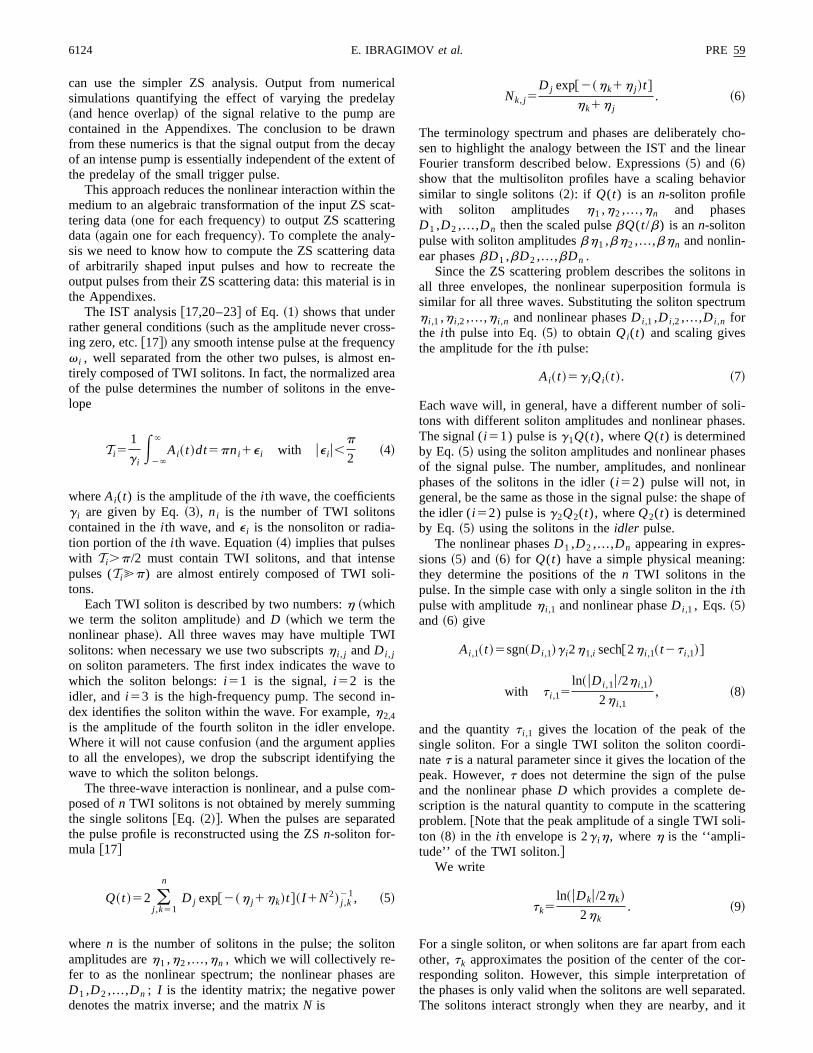
Merely changing the signs of the soliton phasing in tinput pulse gives a 25-fold intensity compression for a fiforder soliton sech pulse. The intensity compression~obtainedby changing all positive phases to alternating phases! for thenth-order soliton sech pulse isn2. However, the secondarextrema in the compressed pulses can contain a signifiportion of the pulse energy: in Fig. 1 the central peakcurvea contains'80% of the total pulse energy, while thsecondary and tertiary peaks bear'13% and 6%, respectively, of the energy of the central peak. The duration ofcentral peak of curvea in Fig. 1 is ' 1
20th that of the sechpulse~curveb!.
Another approach to soliton compression in the TWIsuggested by curvec in Fig. 1. This curve is the profile of thelargest soliton contained in the fifth-order soliton pul~curve b!: the amplitude is 1.8 times that of curveb; the
ns
--
l
-
ntf
e
duration is 19 times that of curveb, and it contains exactly
36% of the energy of curveb. Physically, within a long sechpulse there is always a soliton that has almost twice theplitude of ~and is substantially shorter! than the long sechpulse. In this example, if the largest soliton in the long sepulse can be separated from the other solitons, thenachieve a compression ratio of 9 and a clean intensity disbution, and retain 36% of the energy in the comprespulse.
The synchronously pumped optical parametric oscillaexperiments@6,7# report a compression ratio of 20. Repeaing the computation above shows that for a compressiontio of 20 the central soliton contains 20% of the initial eergy. We believe that this is the type of compressiobserved in Refs.@6,7#.
III. SOLITON SOLUTIONS:SOLITONS IN THE THIRD ENVELOPE
AND NONLINEAR FOURIER TRANSFORM
In many ways, solving a nonlinear equation using an Iis analogous to solving the wave equation using the Foutransform @20–23#. To solve a linear differential equatiousing the Fourier transform, one first decomposes an atrary initial wave into a superposition of simple plane waveThese plane waves do not change during the propagaand so the spectrum is constant: only the phases of the pwaves change during the propagation. To complete the stion to the propagation problem, one computes the nphases from a simple evolution equation, and assemblessolution from the plane waves with their new phases.
Analogous to the linear Fourier transform, in the nonliear case each of the three nonoverlapping input pu@Ai ,0(t), where i 51, 2, and 3, respectively, are the initiasignal, the idler, and the high-frequency pump# can be rep-resented as anonlinearsuperposition ofni solitons with dif-ferent amplitudesh i ,k for 1<k<ni ~which, to emphasize theanalogy with the linear Fourier transform, we refer to as‘‘soliton spectrum’’! with associated nonlinear phasesDi ,kand some residual radiation. As in the linear case, the stons ~in the linear case spectrum! do not change during theinteraction; however, their phases do. To find the shapethe waves after the nonlinear interaction, one needs to cstruct the final envelopes, using the same solitons, but w
FIG. 1. Possible compression for a five-TWI-soliton sech pfile: curve a is the amplitudeA of an alternating phase symmetrfive-soliton profile;b is the amplitudeA of a sech profile with thesame soliton content asa; and c is the amplitudeA of the largestsoliton in b.

t
d
ishe
thoneitoeohao
fen
ealeWa
-
li-taily
atw
is5
oeressas
na
heal
rst
ndrs
-
e
he
naleofnelve
amhe
6126 PRE 59E. IBRAGIMOV et al.
the new phases which the solitons have acquired duringnonlinear interaction.
Suppose that initially there is only an intense pump ansmall signal wave with the highest speedv1 , i.e., the idlerwave with speedv2 is absent before the interaction. Thissimilar to parametric amplification when at the start of tinteraction a small trigger pulse~signal wave! at frequencyv1 is behind an intense pump pulse at frequencyv35v11v2 , and during the interaction the signal overtakespump. Any time the high-frequency pump contains a solitit is unstable. When each pump soliton decays, it emitsactly one soliton into each daughter wave. Thus each solin the pump can be thought of as a bound state of zbinding energy, consisting of a signal and an idler solitwith perfectly matched energies: the matching is exactly tprescribed by the Manley-Rowe relations. The interactionan intense pump with a small trigger pulse breaks the perenergy balance and initiates the decoupling into idler asignal waves@12,13#. During the interaction, all solitons inthe pump split and move to the idler and signal wav@12,13#: the number of solitons in each fundamental equthe number of solitons initially in the pump. However, thphases of each soliton will be changed by the interaction.obtain analytical expressions for the final phases usingapproach developed in Ref.@17#.
When a solitonh3,k in the third envelope splits, it produces two low-frequency solitons: one with amplitudeh1,k inthe first envelope and one with amplitudeh2,k in the secondenvelope with
h1,k5a1h3,k and h2,k5a2h3,k , ~14!
where the scalingsa1 anda2 are
a15n3,2
n2,1and a25
n3,1
n2,1. ~15!
If the n pump solitons areh3,k for 1<k<n, then the signaland idler solitons areh1,k5a1h3,k andh2,k5a2h3,k , respec-tively, for 1<k<n. The nonlinear phases of the output sotons can be computed from an algebraic expressions foroutput scattering matrix. Once the nonlinear phasesknown the dominant soliton portion of the output is readcomputed from the nonlinear superposition@Eqs. ~5! and~6!#.
As Eq.~4! shows, an intense pulse withTi@p/2 is essen-tially composed of TWI solitons sincee i!Ti . We neglectthe radiation~nonsoliton! part of the pump, and assume ththe pump consists entirely of TWI solitons. Figure 2 shorepresentative output from the decay of a 4 sech(t) pumpwith a small trigger pulse: for case 1 the trigger0.05 exp(2t2), while for case 2 the trigger is 0.002exp(2t2). The features to note are that the four solitons@Eq.~13!# contained in the 4 sech(t) pulse have split according tEq. ~14!, and are clearly visible in both the signal and idloutput; the phases in the signal output alternate; the phasthe idler output do not alternate; the most intense soliton ithe lead in both pulses; and smaller trigger pulses increthe separation of the output solitons. The IST theory givevery clear explanation of this behavior. In Ref.@25# we gavean analytical formula describing the behavior of the sig
he
a
e,
x-n
rontfctd
ss
en
here
s
ininsea
l
wave. Here we complete the investigation by including texpressions for the idler. The derivation of the analyticexpressions is in the Appendixes.
The following expressions for the final phases of the fi~signal! and second~idler! solitons in terms of the initialparameters explain the behavior in Fig. 2:
D1,k~ f !5r1~h3,k!2a1h3,k)
j 51j Þk
nh3,k1h3,j
h3,k2h3,jexpF2h1,k
v1zG ,
~16!
D2,k~ f !5r1~h3,k!a2D3,k
~ i ! expF2h2,k
v2zG , ~17!
whereD3,k( i ) are initial phases in the pump,D1,k
( f ) andD2,k( f ) are
final soliton phases in the signal and the idler waves, ah3,1,h3,2,...,h3,k are the initial pump solitons; the parametea1 anda2 are defined in Eq.~15!, andr1 is the ZS reflectioncoefficient of the first~signal! wave. As shown in the Appendixes, if the initial signal pulseA1,0(t) is small, then
r1~h!.1
g1E
2`
`
A1,0~ t !exp~22a1ht !dt. ~18!
When using Eq.~16!, one should bear in mind that due to thway this expression was obtained~see the Appendixes!, thephasesD1,k
( f ) define the final shape of the time reversal of tsignal pulse.
Expressions~16! and ~17! show a dramatic difference inthe behavior of the signal and idler waves. The final sigphasesD1,k
( f ) depend only on the initial soliton content of thpump, anddo notdepend on the initial nonlinear phasesthe pump solitons. This is very surprising: in general owould expect the output shape of the signal wave to invoboth soliton amplitudesh3,k and nonlinear phasesD3,k
( i ) . Alinear analogy to this would be if the propagation of a bedid not depend on the initial shape of its wave front. For tnonlinear case, the fact that Eq.~16! does not involve theinitial nonlinear phasesD3,k
( i ) but only the soliton amplitudes
FIG. 2. Signal and idler amplitudes (A1 andA2) output from thedecay of a four-TWI-soliton@4 sech(t)# pulse: signal and idler 1 arethe output with trigger 0.0025 exp(2t2); signal and idler 2~multi-plied by 21 to make the figure clearer! are the output with trigger0.05 exp(2t2).

c
nr
m
th
re
lsintplppe
oion
i
ndt-
-t
erhtimo
ea
lee
ignaf t
t o
is
di-g
thehich
glep
thig-nalheofndalre
e
ri-a-lecepof
PRE 59 6127THREE-WAVE INTERACTION SOLITONS IN OPTICAL . . .
h3,k means that the output shape of the signal wave pracally does not depend on the initial shape of the pump.
In contrast, the initial phasesD3,k( i ) do appear in expressio
~17! for the final D2,k( f ) idler soliton phases, and the idle
output depends on the initial profiles of the intense pu~through the initial soliton phases! as well as the reflectioncoefficientr(h3,k) ~or radiation spectrum at the pointsh3,k)of the small trigger.
The final shape of the signal depends critically onproduct
Ck5)j 51j Þk
nh3,k1h3,j
h3,k2h3,j, ~19!
which determines the signs of the solitons in Eq.~16!. Thereis no loss of generality in assuming the solitons are ordei.e.,h3,k>h3,k11 , which ensuresC1.0, C2,0, C3.0, etc.It is these alternating signs that give the output signal puthe characteristic profile of a decaying parade of oscillathumps, which can be seen in Fig. 2. In contrast, the ouidler soliton phases@Eq. ~16!# are determined by the initiapump soliton phasesD3,k . If the soliton phases in the pumare initially positive~which is the case for the sech pumpulse in Fig. 2!, then the output idler phase will also bpositive ~as is shown in Fig. 2!.
The exponential factors in Eqs.~16! and ~17! have noinfluence on the output pulse shapes. As discussed abthese exponential factors correspond to uniform translatof the output pulses. In fact, they show that the solitonsEqs.~16! and ~17! move with velocitiesv1 andv2 , respec-tively. Calculating the soliton coordinates~9!—dividing Eq.~16! by twice the soliton amplitude, taking logarithms, adividing again—gives the soliton ‘‘coordinates’’ of the ouput signal and idler solitons (t1,k
( f ) andt2,k( f ) , respectively!
t1,k~ f !5
z
v11
ln r1~h3,k!
2h1,k1
ln~Ck!
2h1,k, ~20!
t2,k~ f !5
z
v21
ln r1~h3,k!
2h2,k1
t3,k~ i !
a2. ~21!
The first terms in Eqs.~20! and~21! arise from the exponential factors in Eqs.~16! and~17!, and show that all the outpuTWI solitons move with the same speed (v1 for the signal,andv2 for the idler!. The second term shows how the triggpulse profileA1,0 effects each soliton in the pump througthe reflection coefficientr1 . When the reflection coefficienis small, the solitons in the signal wave experience large tdelays and the solitons in the idler are advanced. Small stons, corresponding to smallhk , experience larger timeshifts and will be delayed or advanced more by the nonlininteraction: therefore, the generic output signal wave isordered train of TWI solitons, as illustrated in Fig. 2. Smalinitial amplitudes of the signal wave produce bigger timshifts. Figure 2 shows the output for two different input snal intensities: in agreement with theory, the smaller siginput produces longer delays and increased separation ooutput solitons.@Note that Eqs.~16! and~20! give the phasesand coordinates of the time-reversed signal output.# The thirdterms, determined entirely by the pump, show the effec
ti-
p
e
d,
egut
ve,s
n
eli-
arnr
-lhe
f
the other TWI solitons in the pulse: for the signal wave thterm is independent of the coordinatest3,k
( i ) of the input pumppulse. For the idler this term is a scaled copy of the coornates t3,k
( i ) . For small trigger pulses, the terms involvinr(h3,k) are dominant in Eqs.~20! and ~21! and the thirdterms are negligible. This shows that for small triggerstime shift increases as the soliton amplitude decreases wexplains the ordering of the solitons in Fig. 2.
Numerics on system~1!, illustrating the analytical predic-tions, are contained in Figs. 3 and 4. Figure 3 shows a sintrigger pulse with four different pump pulses: all four pumpulses are pure two-soliton profiles withh152.7 andh251, but with different soliton phases. Equations~16! and~17! predict that the signal output of this trigger pulse withese three different pump profiles should be identical. Fure 4 shows the numerical signal and idler output: the sigoutput is the same for the four different pumps, while tidler essentially repeats the pump profile. In practice,course, pulses will never have exact soliton profiles, athere will always be small amounts of radiation. Additionnumerics illustrating the stability of the soliton behavior ain Ref. @25#.
FIG. 3. Initial amplitudes for numerical verification. The puls~t! is the fundamental trigger pulse whilep1 –p4 are pump profiles.All four pump pulses have the same soliton amplitudes (h152.7andh251); they differ in their soliton phases.
FIG. 4. Signal and idler output amplitude from numerical vefication. The pulse~s! is the common signal output predicted anlytically ~the outputs from all four processes are indistinguishab!.The pulsesi1 –i4 are the idler outputs that for the particular choiof trigger with r(2.7)5 r(1.0)51 should reproduce the input pumprofilesp1 –p4 in Fig. 3: the slight deviations are due to the usethe approximate expression forr.
rnaltu
b
espaethe
lle
al,p
ofia
prlsgpuax
ou
f
e
eul-
of
on
iannse
ion
dlheses
lti-estchne
ps
est
theoremps-
his
tric
nur
.
.
6128 PRE 59E. IBRAGIMOV et al.
Expressions~16!–~21! show that the shape of the triggepulse controls the position of the output solitons in the sigand idler waves. In Ref.@25# we showed that for smalGaussian triggers the solitons emerge ordered by ampliin increasing order. In this paper we extend this analysisshow how to adjust the positions of the output solitonschanging the shape of the input trigger pulse.
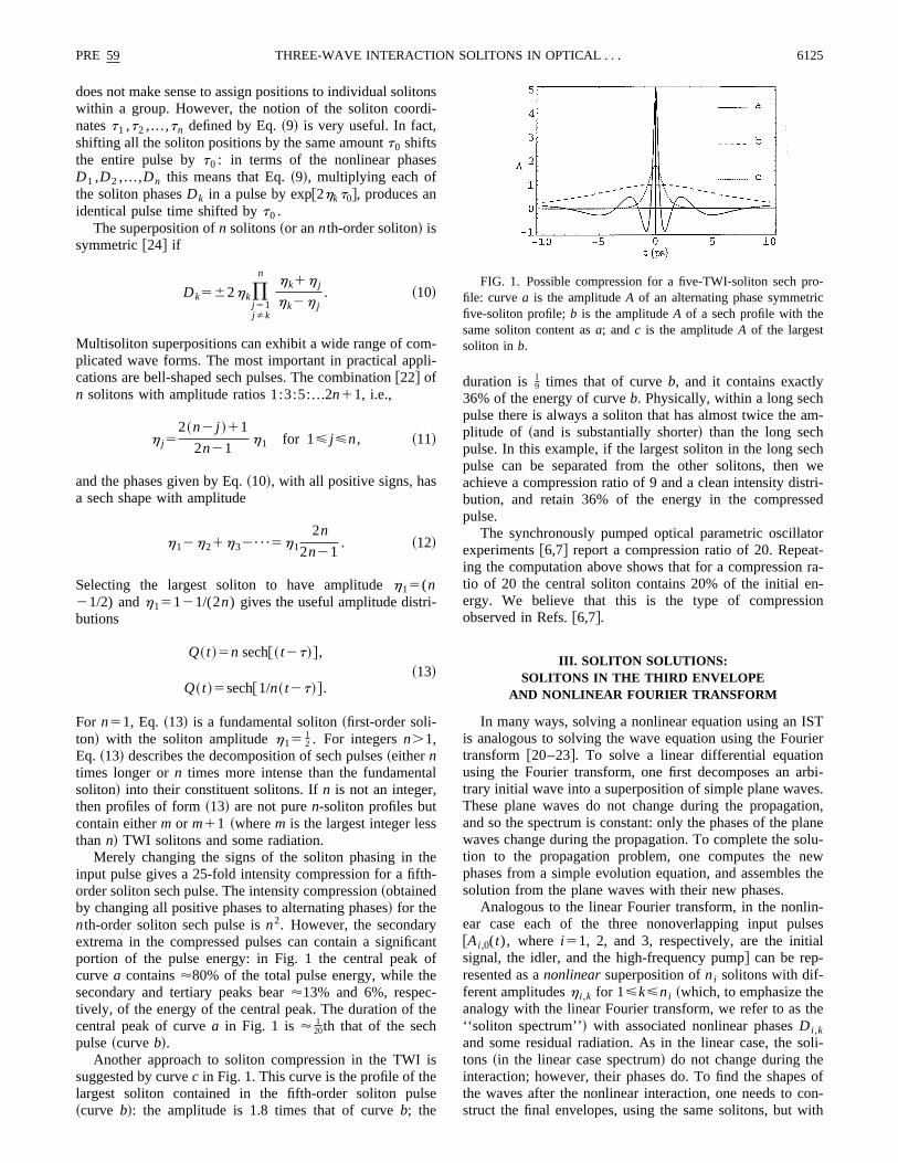
If the parameterr3,k in Eqs. ~20! and ~21! is near zero,then thekth soliton in the signal or idler waves experiencan extreme time shift during the interaction. Since therameterr3,k is determined by the initial signal profile, oncan control the positions of the output solitons by alteringshape of the signal trigger. It is possible to isolate the largsoliton by selecting triggers which delay the other smasolitons. Ifr(h3,k)51 @or, more generally,r5exp(qh1,k) forsomeq# for all pump TWI solitons, then the output signphases@Eq. ~16!# satisfy Eq.~10!, with alternating phaseswhile the output idler phases are a scaled copy of the inphases: in this case the signal output is the symmetric prwith alternating soliton phases and the idler output repethe pump profile. The alternating phases superpositionvides the maximum intensity and compression of the puHowever, these profiles have satellite peaks containinsubstantial fraction of the energy. Note that the idler outrepeats the pump profile when the signal output is the mmal amplitude symmetric profile. Figures 5–7 show somethe possibilities for controlling the shape of the outppulses. Figure 5 shows four different trigger profiles: (t1) is0.2 exp(2t2), which is included to show the typical effect oa moderate trigger; (t2) is (0.450t – 0.112t)exp(2t2), which
FIG. 5. Trigger signal amplitude input for a numerical demostration of the control of soliton positions. The pump for all fotrigger pulses is a two-soliton 2 sech(t) profile.
FIG. 6. Signal amplitude output from triggers 1 and 2 in Fig. 5
l
detoy
-
estr
utletso-e.ati-f
t
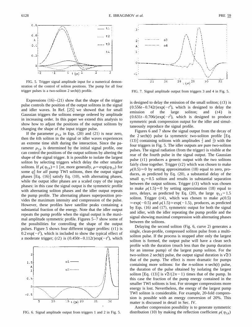
is designed to delay the emission of the small soliton; (t3) is(0.556t – 0.742t)exp(2t2), which is designed to delay themission of the large soliton; and (t4) is(0.631t – 0.706t)exp(2t2), which is designed to producsymmetric peak compression output for the idler and simtaneously reproduce the signal profile.
Figures 6 and 7 show the signal output from the decaythe 2 sech(t) pulse „a symmetric two-soliton profile@Eq.~13!# containing solitons with amplitudes32 and 1
2… with thefour triggers in Fig. 5. The idler outputs are pure two-solitpulses. The signal radiation~from the trigger! is visible at therear of the fourth pulse in the signal output. The Gausspulse (t1) produces a generic output with the two solitofairly close together. Trigger (t2) which was chosen to makr(0.5).0 by setting approximation~18! equal to zero, pro-duces, as predicted by Eq.~20!, a substantial delay of thesmall h250.5 soliton and results in substantial separatbetween the output solitons. Trigger (t3) which was chosento maker(1.5).0 by setting approximation~18! equal tozero, delays, as predicted by Eq.~20!, the largeh3,151.5soliton. Trigger (t4), which was chosen to maker(0.5).exp(20.5) andr(1.5).exp(21.5), produces, as predicteby Eqs.~16! and ~17!, symmetric output for both the signaand idler, with the idler repeating the pump profile and tsignal showing maximal compression with alternating phabetween the solitons.
Delaying the second soliton~Fig. 6, curve 2! generates asingle, clean-profile, compressed soliton pulse from a musoliton pulse. If the process is stopped after only the largsoliton is formed, the output pulse will have a clean seprofile with the duration~much less than the pump duratiofor an intense pump! of the largest pump soliton. For thtwo-soliton 2 sech(t) pulse, the output signal duration is&/3that of the pump. The effect is more dramatic for pumcontaining more solitons: for then-soliton n sech(t) pulse,the duration of the pulse obtained by isolating the largsoliton @Eq. ~13!# is&/(2n21) times that of the pump. Inthis case the fraction of the pump energy contained insmaller TWI solitons is lost. For stronger compressions menergy is lost. Nevertheless, the energy of the largest puTWI soliton is considerable. For example, 20-fold compresion is possible with an energy conversion of 20%. Tmatter is discussed in detail in Sec. IV.
Another compression possibility is to generate symmedistribution~10! by making the reflection coefficientr(h3,k)
-
FIG. 7. Signal amplitude output from triggers 3 and 4 in Fig. 5
ro
ell
thin
in-pa
on
estrritin
eerepe-
e
e
toraetrirthanis
nisscunig
dn
yec
isave
eto-
er-
pris--
thenot
esen
the
menu-
areati-STin-allye isthisionofileof a
-
-
entst
hefor
thend
itonous
PRE 59 6129THREE-WAVE INTERACTION SOLITONS IN OPTICAL . . .
equal to 1 simultaneously for all the pump solitons to pduce the peak soliton interaction~Figs. 5 and 7, curves 4!.This generates stronger compression at the cost of satpulses. For the two-soliton 2 sech(t) pulse in Fig. 7 (s4), theoutput signal amplitude is about three times greater thanof the pump. The effect is more dramatic for pumps containg more solitons: for then-soliton n sech(t) pulse, the am-plitude compression by creating the optimal alternatphases@Eq. ~10!# is close ton times with a very short duration. Although energy conversion is high in this second tyof compression, the appearance of satellite pulses is a mdrawback.
IV. EXPERIMENTAL OBSERVATIONOF TWI-SOLITON BEHAVIOR
In this section we compare predictions of the TWI-solittheory with the experimental results observed in Refs.@6,7#for an experimental synchronously pumped optical paramric oscillator~SPOPO!. Dispersion is extremely small in thiSPOPO, and the observed soliton behavior cannot be atuted to the well-known cascaded quadratic nonlinea(x (2)3x (2)) soliton like waves which can appear onlystrongly dispersive quadratic media.
There is difference between the notation of the prespaper and Refs.@6,7#. The present paper considers paramric amplification which corresponds to the steady-stategime in the SPOPO. In the theoretical section of this pathe ‘‘signal’’ refers to the trigger wave initially present before the interaction. In Refs.@6,7#, the signal wave refers tothe highest frequency~and intermediate speed! fundamentalwave. To avoid confusion we will continue to refer to thfastest fundamental wave as the signal.
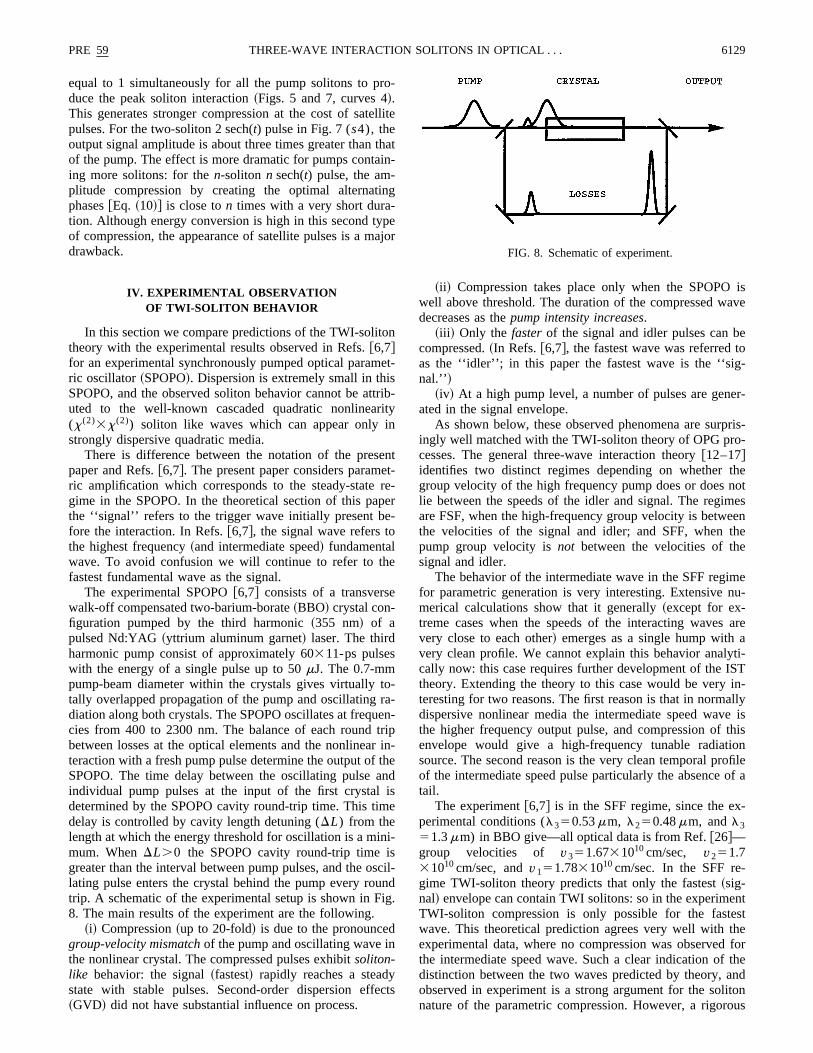
The experimental SPOPO@6,7# consists of a transverswalk-off compensated two-barium-borate~BBO! crystal con-figuration pumped by the third harmonic~355 nm! of apulsed Nd:YAG~yttrium aluminum garnet! laser. The thirdharmonic pump consist of approximately 60311-ps pulseswith the energy of a single pulse up to 50mJ. The 0.7-mmpump-beam diameter within the crystals gives virtuallytally overlapped propagation of the pump and oscillatingdiation along both crystals. The SPOPO oscillates at frequcies from 400 to 2300 nm. The balance of each roundbetween losses at the optical elements and the nonlineateraction with a fresh pump pulse determine the output ofSPOPO. The time delay between the oscillating pulseindividual pump pulses at the input of the first crystaldetermined by the SPOPO cavity round-trip time. This timdelay is controlled by cavity length detuning (DL) from thelength at which the energy threshold for oscillation is a mimum. WhenDL.0 the SPOPO cavity round-trip time igreater than the interval between pump pulses, and the olating pulse enters the crystal behind the pump every rotrip. A schematic of the experimental setup is shown in F8. The main results of the experiment are the following.
~i! Compression~up to 20-fold! is due to the pronouncegroup-velocity mismatchof the pump and oscillating wave ithe nonlinear crystal. The compressed pulses exhibitsoliton-like behavior: the signal~fastest! rapidly reaches a steadstate with stable pulses. Second-order dispersion eff~GVD! did not have substantial influence on process.
-
ite
at-
g
ejor
t-
ib-y
ntt--r
--n-pin-ed
e
-
il-d.
ts
~ii ! Compression takes place only when the SPOPOwell above threshold. The duration of the compressed wdecreases as thepump intensity increases.
~iii ! Only the fasterof the signal and idler pulses can bcompressed.~In Refs.@6,7#, the fastest wave was referredas the ‘‘idler’’; in this paper the fastest wave is the ‘‘signal.’’!
~iv! At a high pump level, a number of pulses are genated in the signal envelope.
As shown below, these observed phenomena are suringly well matched with the TWI-soliton theory of OPG processes. The general three-wave interaction theory@12–17#identifies two distinct regimes depending on whethergroup velocity of the high frequency pump does or doeslie between the speeds of the idler and signal. The regimare FSF, when the high-frequency group velocity is betwethe velocities of the signal and idler; and SFF, whenpump group velocity isnot between the velocities of thesignal and idler.
The behavior of the intermediate wave in the SFF regifor parametric generation is very interesting. Extensivemerical calculations show that it generally~except for ex-treme cases when the speeds of the interacting wavesvery close to each other! emerges as a single hump withvery clean profile. We cannot explain this behavior analycally now: this case requires further development of the Itheory. Extending the theory to this case would be veryteresting for two reasons. The first reason is that in normdispersive nonlinear media the intermediate speed wavthe higher frequency output pulse, and compression ofenvelope would give a high-frequency tunable radiatsource. The second reason is the very clean temporal prof the intermediate speed pulse particularly the absencetail.
The experiment@6,7# is in the SFF regime, since the experimental conditions (l350.53mm, l250.48mm, andl351.3mm) in BBO give—all optical data is from Ref.@26#—group velocities of v351.6731010cm/sec, v251.731010cm/sec, andv151.7831010cm/sec. In the SFF regime TWI-soliton theory predicts that only the fastest~sig-nal! envelope can contain TWI solitons: so in the experimTWI-soliton compression is only possible for the fastewave. This theoretical prediction agrees very well with texperimental data, where no compression was observedthe intermediate speed wave. Such a clear indication ofdistinction between the two waves predicted by theory, aobserved in experiment is a strong argument for the solnature of the parametric compression. However, a rigor
FIG. 8. Schematic of experiment.

yta
l aac
eeth
thimg
ca
thetheude,he
F
esof
eryhav-
tricler
ng-
d-
vesve a
inr of
ob-s.filetheumppedasesF
u.F
go
6130 PRE 59E. IBRAGIMOV et al.
analysis of the experiment requires the complete analtheory for the SFF regime: unfortunately this theory is notadvanced as FSF theory. We anticipate future theoreticavances will provide the analytical tools to complete an exquantitative picture of the SFF process.
Here we attempt to explain the SFF process qualitativusing the well-developed FSF theory. Our qualitative dscription is based on the numerically observed fact thatbehavior of the fastest wave~which can carry TWI solitons!in the SFF regime is surprisingly close to the behavior offastest wave in an associated FSF regime: the FSF reg‘‘corresponding’’ to a SFF regime is obtained by interchaning the group velocities of the idler and the pump. Numericalculations show that the output shape of the fastest~signal!
FIG. 9. Comparison of the signal and idler amplitude outpfrom the decay of a 2 sech(t/4) pump in different velocity regimesSignal and idler 1 are the SFF case. Signal and idler 2 are thesoliton decay case. In both cases the pump is 2 sech(t/4), the triggeris 0.05 sech(t), and the frame of reference is moving at the averaof the extreme velocities. Note the marked qualitative similaritythe leftmost portion of the signal curves.
icsd-t
ly-e
ee
-l
wave are very close for these two cases. In fact, wheninitial shape of the pump is Gaussian, the output shape offastest wave is always the sequence of decreasing-amplitoscillating humps predicted by the rigorous FSF theory. Tarea of the first hump~which is the largest soliton in the FScase but isnot a soliton in the SFF case! is within a fewpercent ofp in the SFF case. However, the following pulshave areas considerably smaller than the ‘‘soliton area’’p. The height and duration of the leading pulse are also vclose for the corresponding SFF and FSF cases. The beior of the slower~idler! wave is completely different for theSFF and FSF cases.
Figure 9 compares numerical simulations of parameamplification in the FSF and SFF regimes: signal 1 and id1 are from the experimental SFF parametersv351.6731010, v251.7131010, and v151.7831010; signal 2 andidler 2 are from the FSF parameters obtained by interchaing v2 and v3 , i.e., v251.6731010, v351.7131010, andv151.7831010. Note that the signal pulses~particularly themost intense lefthand portions! are similar in both cases, anthat idler 1~as predicted by theory! does not have the distinguishing solitons characteristics of idler 2.
This analogy between the behavior of the fastest wafor the SFF and associated FSF regimes allows us to giqualitative explanation of the behavior of the fastest wavethe SFF case by using the FSF theory. In the remaindethis section we describe the behavior of the fastest~signal!wave by considering the corresponding FSF regime,tained by switching the idler and pump group velocitieTables I and II summarize the soliton content of sech propump pulses for the corresponding FSF regime in whichpump wave contains solitons. In the FSF case these psolitons split and emerge according to the theory develoearlier in this paper: the lead pulses in the SFF and FSF care qualitatively similar. The similarity between the two FS
t
SF
ef
thaking the
TABLE I. Soliton content ofn sech(t) pump pulses~FSF regime!. The first three columns contain the peak amplitude, width, full widat half maximum of intensity~FWHMI!, and soliton content@Eq. ~13!# of ann sech(t) pump pulse. The next two columns contain the peamplitude and width~FWHMI! of the largest soliton in the pump; the adjacent columns contain the compression obtained by isolatlargest soliton and the percent of the pump energy it contains. The last column is the amplitude~twice the sum of the solitons! of the pulseformed from the same solitons with symmetric alternating phases@Eq. ~10!#.
n
n sech(t)pump
Largestsoliton Alternating
phasesAmp.Amp. Width h’s Amp. Width Comp. Energy %
1 1 1.7621
21 1.762 1 100 1
2 2 1.7621
2,3
23 0.587 3 75 4
3 3 1.7621
2,3
2,5
25 0.3 52 5 56 9
4 4 1.7621
2,3
2,5
2,7
27 0.652 7 44 16
5 5 1.7621
2,3
2,5
2,7
2,9
29 0.696 9 36 25
n n 1.7621
2,3
2,...,n2
1
22n21
1.762
~2 n21!2n21 100S 2
n2
1
n2D n2
ent of theth
PRE 59 6131THREE-WAVE INTERACTION SOLITONS IN OPTICAL . . .
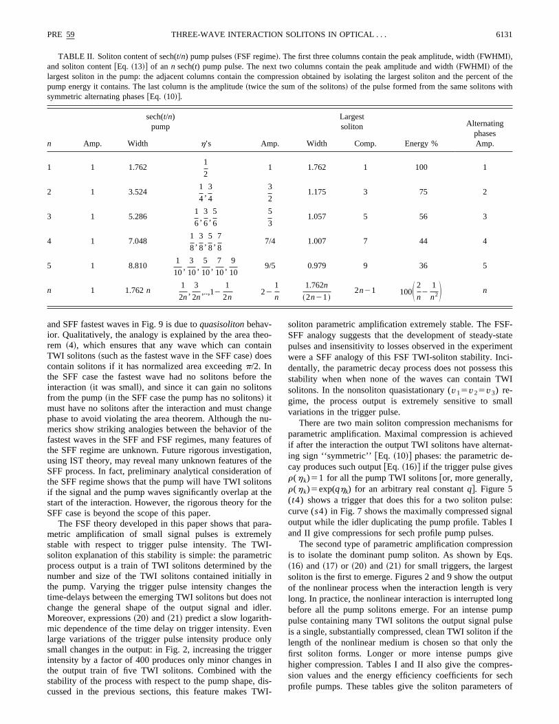
TABLE II. Soliton content of sech(t/n) pump pulses~FSF regime!. The first three columns contain the peak amplitude, width~FWHMI!,and soliton content@Eq. ~13!# of an n sech(t) pump pulse. The next two columns contain the peak amplitude and width~FWHMI! of thelargest soliton in the pump: the adjacent columns contain the compression obtained by isolating the largest soliton and the percpump energy it contains. The last column is the amplitude~twice the sum of the solitons! of the pulse formed from the same solitons wisymmetric alternating phases@Eq. ~10!#.
n
sech(t/n)pump
Largestsoliton Alternating
phasesAmp.Amp. Width h’s Amp. Width Comp. Energy %
1 1 1.7621
21 1.762 1 100 1
2 1 3.5241
4,3
4
3
21.175 3 75 2
3 1 5.2861
6,3
6,5
6
5
31.057 5 56 3
4 1 7.0481
8,3
8,5
8,7
87/4 1.007 7 44 4
5 1 8.8101
10,
3
10,
5
10,
7
10,
9
109/5 0.979 9 36 5
n 1 1.762n1
2n,
3
2n,..,12
1
2n22
1
n
1.762n
~2n21!2n21 100S 2
n2
1
n2D n
eoai
ts
nnuths
iotho
nthth
arlyI
ricthinthnle
enlge
iediW
F-stateenti-this
WI
all
foredat--
se:alI
ionqs.ttputeryngmplsethethevees-echs of
and SFF fastest waves in Fig. 9 is due toquasisolitonbehav-ior. Qualitatively, the analogy is explained by the area threm ~4!, which ensures that any wave which can contTWI solitons~such as the fastest wave in the SFF case! doescontain solitons if it has normalized area exceedingp/2. Inthe SFF case the fastest wave had no solitons beforeinteraction~it was small!, and since it can gain no solitonfrom the pump~in the SFF case the pump has no solitons! itmust have no solitons after the interaction and must chaphase to avoid violating the area theorem. Although themerics show striking analogies between the behavior offastest waves in the SFF and FSF regimes, many featurethe SFF regime are unknown. Future rigorous investigatusing IST theory, may reveal many unknown features ofSFF process. In fact, preliminary analytical considerationthe SFF regime shows that the pump will have TWI solitoif the signal and the pump waves significantly overlap atstart of the interaction. However, the rigorous theory forSFF case is beyond the scope of this paper.
The FSF theory developed in this paper shows that pmetric amplification of small signal pulses is extremestable with respect to trigger pulse intensity. The TWsoliton explanation of this stability is simple: the parametprocess output is a train of TWI solitons determined bynumber and size of the TWI solitons contained initiallythe pump. Varying the trigger pulse intensity changestime-delays between the emerging TWI solitons but doeschange the general shape of the output signal and idMoreover, expressions~20! and~21! predict a slow logarith-mic dependence of the time delay on trigger intensity. Evlarge variations of the trigger pulse intensity produce osmall changes in the output: in Fig. 2, increasing the trigintensity by a factor of 400 produces only minor changesthe output train of five TWI solitons. Combined with thstability of the process with respect to the pump shape,cussed in the previous sections, this feature makes T
-n
he
ge-eof
n,ef
see
a-
-
e
eotr.
nyr
n
s-I-
soliton parametric amplification extremely stable. The FSSFF analogy suggests that the development of steady-pulses and insensitivity to losses observed in the experimwere a SFF analogy of this FSF TWI-soliton stability. Incdentally, the parametric decay process does not possessstability when when none of the waves can contain Tsolitons. In the nonsoliton quasistationary (v15v25v3) re-gime, the process output is extremely sensitive to smvariations in the trigger pulse.
There are two main soliton compression mechanismsparametric amplification. Maximal compression is achievif after the interaction the output TWI solitons have alterning sign ‘‘symmetric’’ @Eq. ~10!# phases: the parametric decay produces such output@Eq. ~16!# if the trigger pulse givesr(hk)51 for all the pump TWI solitons@or, more generally,r(hk)5exp(qhk) for an arbitrary real constantq#. Figure 5(t4) shows a trigger that does this for a two soliton pulcurve (s4) in Fig. 7 shows the maximally compressed signoutput while the idler duplicating the pump profile. Tablesand II give compressions for sech profile pump pulses.
The second type of parametric amplification compressis to isolate the dominant pump soliton. As shown by E~16! and ~17! or ~20! and ~21! for small triggers, the largessoliton is the first to emerge. Figures 2 and 9 show the ouof the nonlinear process when the interaction length is vlong. In practice, the nonlinear interaction is interrupted lobefore all the pump solitons emerge. For an intense pupulse containing many TWI solitons the output signal puis a single, substantially compressed, clean TWI soliton iflength of the nonlinear medium is chosen so that onlyfirst soliton forms. Longer or more intense pumps gihigher compression. Tables I and II also give the comprsion values and the energy efficiency coefficients for sprofile pumps. These tables give the soliton parameter

6132 PRE 59E. IBRAGIMOV et al.
TABLE III. Parameters for comparison of theory and experiment.
Phase matching Idler Signal Pumpangle~degrees! l1 mm v1 cm/sec l2 mm v2 cm/sec l3 mm v3 cm/sec
Case 1 27 1.80 1.7831010 0.43 1.7031010 0.35 1.6731010
Case 2 30 1.30 1.7931010 0.47 1.7231010 0.35 1.6831010
nze
caatep
ata
IatWeTtrrg
ggpthilo
tthcalet
nd
liarth
itinolis-st
iab
m
li-rgrtfr
obgthin
ed
/V.ingoli-ontwoal-
plifi-ofFort inory
hees;sta-
is
the
-ap-theel-
forfile.oli-the
ng
ent
the largest TWI soliton contained in pump. After this solitomoves to the signal wave its amplitude must be normaliaccording to relationships~14! and~15! and then~2! and~3!.This normalization is important and in extreme casessubstantially alter the results. However, in the general cwhen the speeds of the three waves are well separaTables I and II give a good idea about the compressionrameters.
A very attractive feature of compressing pulse by isoling the largest soliton is that the compression appears nrally: for small Gaussian trigger pulses Eqs.~16! and ~17!show that the largest TWI soliton always emerges first.practice, however, it is difficult to stop the interactionexactly the right moment, and a second and even a third Tsoliton may also form: although this increases the procefficiency, it spoils the shape of the compressed pulse.obtain cleaner output pulses, one should use less intenseger pulses by introducing losses into the resonator: lalosses in the resonator decrease the intensity of the tripulses and increase the separation of the output solitonsducing cleaner output. This behavior was observed inexperiment. Another way to obtain clean pulses is to tathe shape of the input signal pulse. Section III shows howproduce pulse profiles by designing the trigger to delayappearance of the smaller TWI solitons. This techniqueproduce compressed pulses with very clean sech profiCurve (t2) in Fig. 5 is the trigger giving the signal outpu(s2) in Fig. 6: the smaller soliton is strongly delayed, aboth the signal and idler output are clean.
Tables I and II show that the intensity of the largest soton is approximately twice the pump intensity when theremore than three pump TWI solitons, and the duration oflargest soliton decreases rapidly as the pump energycreases. The primary drawback of compressing by isolathe largest soliton is that only the energy of the largest ston is used~the pump energy in the smaller solitons is dcarded!, and the efficiency drops for high compressionHowever, as the tables show, even for high compressionslargest soliton contains a significant portion of the initpump energy. For example, ninefold compression canachieved with an energy efficiency of 36%, and 20-fold copression with 20% efficiency.~Efficiency is defined as thefraction of the initial pump energy in the largest TWI soton.! Note: 100% efficiency means that all the pump eneis transformed into the signal and idler. This energy is pationed between the generated waves according to theirquencies and normalizations~2! and ~3! and ~14! and ~15!.
The experimental compression of the fastest waveserved in Refs.@6,7# was analogous in behavior to isolatinof the largest TWI soliton. We compared the theory andexperiment at two different frequencies and phase matchangles. The parameters for the two cases are summarizTable III. All the data are taken from Ref.@26#, which gives
d
nsed,
a-
-tu-
n
Issoig-eerro-eroens.
-een-gi-
.hele-
yi-e-
-
egin
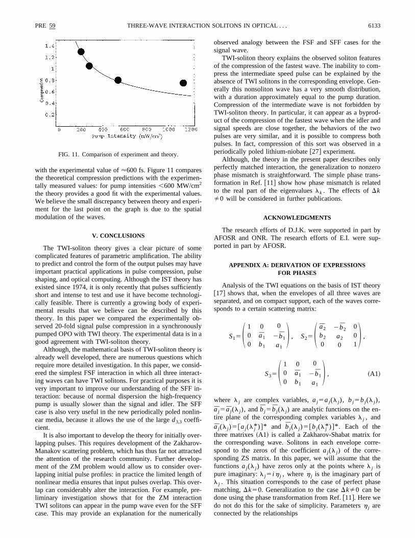
the appropriate nonlinear coefficient for BBO as 2.3 pmEstimating the pump energy shows that in the correspondFSF case each pump pulse could contain 10–15 TWI stons. Tables I and II predict that the largest pump solitshould be 20–30 times shorter than the pump. There arefactors that need to be accounted for: the first is the normizations ~14! and ~15! describing the transfer of the pumTWI soliton to another envelope; the second is the ampcation and compression which results from the proximityTWI solitons in the train when the phases are alternating.the experimental frequencies in BBO, these factors acopposite directions, and approximately cancel. The thepredicts a compression of;20 for a pump intensity of;800MW/cm2, exactly what is observed in the experiment. Ttheory predicts higher compression for higher intensitihowever, in the experiment the compression coefficientbilized after the pump intensity reached 800 MW/cm2. Webelieve this to be due to spatial pulse modulation, whichneglected in the theory.
In the experiments the nonlinear medium was roughlylength required for the first TWI soliton to form. For lowintensity pumps@Fig. 10~B!# the profile is clean without satellites because only the most intense TWI soliton haspeared: the compression is roughly a factor of 12. Aspump intensity increases the temporal output profile devops additional maxima@compare Fig. 10~A! with Figs. 2 or9# because the nonlinear medium is now sufficiently longthe less intense solitons to form and spoil the clean proTheory predicts that the duration of the dominant pump ston should be inversely proportional to the square root ofpump intensity. The 0.7-mJ pulse@Fig. 10~B!# has a durationof t'850 fs. Computing the proportionality constant usithis value gives a prediction that the 1.8 mJ [email protected]~A!# should have a duration of 530 fs, in good agreem
FIG. 10. Experimental results.
sen
esetia
elitavlsatllorithobusn
ishisidc
itinncFlin
r-oteopr-
ofvernFll
r the
resm-
theen-n,n.byd-andtwoothn a
nlyerons-d
byp-
ryareorre-
-
rrre-
the
ase
PRE 59 6133THREE-WAVE INTERACTION SOLITONS IN OPTICAL . . .
with the experimental value of'600 fs. Figure 11 comparethe theoretical compression predictions with the experimtally measured values: for pump intensities,600 MW/cm2
the theory provides a good fit with the experimental valuWe believe the small discrepancy between theory and expment for the last point on the graph is due to the spamodulation of the waves.
V. CONCLUSIONS
The TWI-soliton theory gives a clear picture of somcomplicated features of parametric amplification. The abito predict and control the form of the output pulses may himportant practical applications in pulse compression, pushaping, and optical computing. Although the IST theory hexisted since 1974, it is only recently that pulses sufficienshort and intense to test and use it have become technocally feasible. There is currently a growing body of expemental results that we believe can be described bytheory. In this paper we compared the experimentallyserved 20-fold signal pulse compression in a synchronopumped OPO with TWI theory. The experimental data is igood agreement with TWI-soliton theory.
Although, the mathematical basis of TWI-soliton theoryalready well developed, there are numerous questions wrequire more detailed investigation. In this paper, we conered the simplest FSF interaction in which all three interaing waves can have TWI solitons. For practical purposesvery important to improve our understanding of the SFFteraction: because of normal dispersion the high-frequepump is usually slower than the signal and idler. The Scase is also very useful in the new periodically poled nonear media, because it allows the use of the larged3,3 coeffi-cient.
It is also important to develop the theory for initially ovelapping pulses. This requires development of the ZakharManakov scattering problem, which has thus far not attracthe attention of the research community. Further develment of the ZM problem would allow us to consider ovelapping initial pulse profiles: in practice the limited lengthnonlinear media ensures that input pulses overlap. This olap can considerably alter the interaction. For example, pliminary investigation shows that for the ZM interactioTWI solitons can appear in the pump wave even for the Scase. This may provide an explanation for the numerica
FIG. 11. Comparison of experiment and theory.
-
.ri-l
yeesygi--is-lya
ch-
t-is-y
F-
v-d-
r-e-
Fy
observed analogy between the FSF and SFF cases fosignal wave.
TWI-soliton theory explains the observed soliton featuof the compression of the fastest wave. The inability to copress the intermediate speed pulse can be explained byabsence of TWI solitons in the corresponding envelope. Gerally this nonsoliton wave has a very smooth distributiowith a duration approximately equal to the pump duratioCompression of the intermediate wave is not forbiddenTWI-soliton theory. In particular, it can appear as a byprouct of the compression of the fastest wave when the idlersignal speeds are close together, the behaviors of thepulses are very similar, and it is possible to compress bpulses. In fact, compression of this sort was observed iperiodically poled lithium-niobate@27# experiment.
Although, the theory in the present paper describes operfectly matched interaction, the generalization to nonzphase mismatch is straightforward. The simple phase traformation in Ref.@11# show how phase mismatch is relateto the real part of the eigenvalueslk . The effects ofDkÞ0 will be considered in further publications.
ACKNOWLEDGMENTS
The research efforts of D.J.K. were supported in partAFOSR and ONR. The research efforts of E.I. were suported in part by AFOSR.
APPENDIX A: DERIVATION OF EXPRESSIONSFOR PHASES
Analysis of the TWI equations on the basis of IST theo@17# shows that, when the envelopes of all three wavesseparated, and on compact support, each of the waves csponds to a certain scattering matrix:
S15S 100
0a1
b1
0
2b1
a1
D , S25S a2
b2
0
2b2
a2
0
001D ,
S35S 100
0a1
b1
0
2b1
a1
D , ~A1!
where l j are complex variables,aj5aj (l j ), bj5bj (l j ),a j5a j (l j ), andb j5b j (l j ) are analytic functions on the entire plane of the corresponding complex variablesl j , anda j (l j )5@aj (l j* )#* and b j (l j )5@bj (l j* )#* . Each of thethree matrixes~A1! is called a Zakharov-Shabat matrix fothe corresponding wave. Solitons in each envelope cospond to the zeros of the coefficientaj (l j ) of the corre-sponding ZS matrix. In this paper, we will assume thatfunctionsaj (l j ) have zeros only at the points wherel j ispure imaginary:l j5 ih j , whereh j is the imaginary part ofl j . This situation corresponds to the case of perfect phmatching,Dk50. Generalization to the caseDkÞ0 can bedone using the phase transformation from Ref.@11#. Here wedo not do this for the sake of simplicity. Parametersh j areconnected by the relationships
te
thngth
veby
-
a
eeio
i-er
de
eIf
ve
e
s.
ain,s are
trixhe
ix:
ffi-
to
i-
t of
themwilln, a
ithi-
ialact,
ues-to
6134 PRE 59E. IBRAGIMOV et al.
h15n3,2
n2,1h35a1h3 , ~A2!
h25n3,1
n2,1h35a2h3 . ~A3!
Each of the functionsaj (h j ) are assumed to have a fininumber of zeros,h j ,k . The value of h j ,k for whichaj (h j ,k)50 gives the amplitude of thekth soliton in thej thenvelope. As described above, solitons can move frompump to the signal and idler and back. When solitons chaenvelopes, their amplitudes must be normalized. If beforeinteraction the pump hadn TWI solitons with amplitudesh3,k , then after the interaction the signal and the idler wawill receive these solitons with their amplitudes dictatedthe relationships
h1,k5n3,2
n2,1h3,k5a1h3,k , ~A4!
h2,k5n3,1
n2,1h3,k5a2h3,k . ~A5!
This means that ifa3(h) in the beginning of the interactionhas zeros at the pointsh3,k , after the interaction, the elementsa1(h) anda2(h) will have zeros at the pointsh1,k andh2,k connected with the pump solitons with the normaliztions ~A4! and ~A5!.
To find the final soliton phases, we need to obtain exprsions of the ratiosbj /aj for each wave at the end of thinteraction. Such ratios in IST theory are called reflectcoefficients. At each point whereaj becomes zero,bj /aj hasa pole. Soliton phasesD j ,k can be obtained by taking resdues of the reflection coefficients at those points whaj (h j ,k)50. Such poles correspond to TWI solitons.~Hereindex j corresponds to the number of the envelope, and ink corresponds to the soliton number.! The overall scatteringmatrix S for the TWI problem is the product of the thrematrixes corresponding to each of the interacting waves.the beginning of the interaction (z→2`,t→2`) the sec-ond wave was in the front of the third and the first wafollowed the third, then
S~ i !5S2~ i !S3
~ i !S1~ i ! , ~A6!
where the indexi stands for ‘‘initial.’’ ~Notice that our no-tations are different from that in Ref.@17#.! Due to the dif-ferences between the speeds, the waves reorder after thteraction:
S~ f !5S1~ f !S3
~ f !S2~ f ! , ~A7!
where an indexf stands for ‘‘final.’’ The order of the finalscattering matricesS( f ) reflects the reordering of the pulseThe evolution of the elementsan,m of the scattering matrixSis given by the expression@17#
an,m~l,z!5an,m~l,0!expF2 ilzS vm2vn
v1v2v3D G , ~A8!
eee
s
-
s-
n
e
x
in
in-
wherev i are the group speeds of the waves. Notice agthat in the present paper, the time and space coordinateinterchanged as compared with the work@17#. Expression~A8! enables us to relate the elements of the scattering mabefore and after the interaction. If in the beginning of tinteraction, the wave with the smallest velocityv2 was ab-sent~the fastest wave withv1 is the signal wave!, then thecorresponding ZS matrix for this wave is the identity matra2
( i )5a2( i )51 and b2
( i )5b2( i )50. EquatingS( i ) and S( f ) for
this case, we obtain the expression for the reflection coecient r2(l) for the idler wave:
b2~ f !
a2~ f ! 5
b3~ i !b1
~ i !
a3~ f !a2
~ f ! expF2h2
v2zG
or
r25b2
~ f !
a2~ f ! 5
b3~ i !
a3~ i ! b1
~ i ! expF2h2
v2zG . ~A9!
Here we used the relationshipa2( f )a3
( f )5a2( i )a3
( i ) .To obtain the final phases of the idler wave, one has
find the residues of the reflection coefficient~A9! at thepoints h2,k connected with the initial pump soliton ampltudesh3,k by relationships~A5!:
D2,k~ f !5
2 ib3~ i !~h3!
d
dh2a3
~ i !~h3!uh25h2,k
b1~ i ! expF2
h2
v2zG
5a2D3,k~ i ! b1
~ i ! expF2h2
v2zG ; ~A10!
when taking derivatives, we again used expression~A5!.The analogous expression for the reflection coefficien
the signal wave with the largest velocityv1 cannot be ob-tained from Eqs.~A1!–~A7! directly. To find the reflectioncoefficients for this case, we use the fact that ifAj (t,z) aresolutions of system~1!, then the functions2Aj (2t,2z) arealso solutions of the same system. The final result ofdirect problem will serve as initial conditions for the probleinverted in time and space, and vice versa. Therefore weconsider a process where, at the end of the interactiosmall signal waveA1(t) with a speedv1 is in the front of alarge pump waveA3(t) with no idler wave. The initial con-ditions for this reversed process will be a signal wave wthe amplitudeA1(2t) chasing a large pump with the ampltudeA3(2t) with no idler wave. The final coefficientsa andb for such an inverted process will be equal to the initvalues of the direct process, and vice versa. Using this fwe obtain
b1~ f !
a1~ f ! 5
b1~ i !
a1~ i !a3
~ i ! expF2h1,k
v1zG . ~A11!
The final soliton phases can be obtained by taking residof the functions~A9! and ~A11! at the points where coefficientsa anda of the corresponding ZS matrices are equalzero:

th
p-
ter-n.
PRE 59 6135THREE-WAVE INTERACTION SOLITONS IN OPTICAL . . .
D1,k~ f !5
b1~ i !~h1!
a1~ i !
d
dh1@a3
~ i !~h3!#uh15h1,k
expF22h1,k
v1zG .
~A12!
Notice that the differentiation here is done with respect tovariableh1 , but that the coefficienta3(h3) is a function ofh3 . The connection betweenh1 andh3 is given by relations~A4! and ~A5!. Expression~4! shows that an intense pumwave consist almost entirely of TWI solitons. In the follow
u
lo
aoblltt
m
e
ing analysis, we will assume that the pump before the inaction consisted only of TWI solitons and had no radiatioIn this case the coefficientsa3(h) can be written as
a3~h3!5)k51
nh32h3,k
h31h3,k, ~A13!
whereh3,k is as usual the amplitude of thekth soliton in thepump. Differentiating Eq.~A13! with respect toh1 and usingrelationship~A2! we obtain
d
dh1F)
j 51
nh32h3,j
h31h3,jGU
h15h1,k
51
a1
d
dh3F )
k51
nh32h3,j
h31h3,jGU
h35h3,k
51
2a1h3,k)j 51j Þk
nh3,k2h3,j
h3,k1h3,j. ~A14!
.onare
he
em
-e
lf
Notice that the derivative of the product in Eq.~A14! hasonly one nonzero term at the pointsh35h3,k . After a sub-stitution of Eq.~A14! into expression~A12!, we obtain theexpression for the final phases of the signal wave:
D1,k~ f !5S b1
~ i !
a1~ i !D 2a1h3,k)
j 51j Þk
nh3,k1h3,j
h3,k2h3,jexpF2
h1,k
v1zG .
~A15!
One should be careful when using expression~A15!. Be-cause this formula was obtained by reversing time, the oput shape of the signal wave determined by Eq.~A15! willalso be reversed in time.
APPENDIX B: ZAKHAROV-SHABAT PROBLEMAND REFLECTION COEFFICIENTS
Expressions~A10! and~A15! connect the initial and finascattering data for the parametric amplification process. Bexpressions contain parametersa and b from Zakharov-Shabat scattering matrixes~A1!. In this appendix we showthe connection between these coefficients and the initial d
The connection is based on the direct ZM scattering prlem @17# scattering problem. When the pulses are physicaseparated, as they are before the interaction, the ZM scaing problem reduces to a set of three~one for each pulse! ZSscattering problems
ui81 ilui5qi~ t !v i ,~B1!
v i82 ilv i52qi* ~ t !ui ,
with potentialqi(t) given by
qi~ t !51
g iAi ,0* ~ t !. ~B2!
The functionsu andv are the eigenfunctions and the paraetersl the eigenvalues of the ZS problem~B1!.
If potential ~B2! decreases sufficiently rapidly ast→6` that
t-
th
ta.-
yer-
-
E2`
`
uqi~ t !uekutudt,` ~B3!
for any positive numberk, then all solutions of system~B1!are asymptotic ast→6` to simple exponential functions~Clearly, this assumption imposes no physical restrictionsthe pulses that can be considered since all optical pulsesbounded in both time and space.! Moreover, any solution ofEq. ~B1! can be written either as a linear combination of ttwo solutionsf and f system~B1! satisfying
f→F10Ge2 ilt, f→F 021Geilt when t→2`, ~B4!
or as linear combinations of the two solutionsc and c sat-isfying
c→F01Geilt, c→F10Ge2 ilt when t→1`, ~B5!
where we have omitted the indexi for clarity. Either pair offunctions forms a complete set of solutions of the syst~B1!. So the first pair of solutions~B4! are a linear combi-nation of the the second pair~B5!, i.e.,
f5ac1bc→S ab
e2 ilt
eilt D as t→1`,
f5bc2ac→S b2a
e2 ilt
eilt D as t→1`. ~B6!
The coefficientsa, b, a, andb ~which depend upon the spectral parameterl! relating the two sets of solutions form thZakharov-Shabat scattering matrix
SZS5S a~l!,b~l!,
2b~l!
a~l!D . ~B7!
In Ref. @23# it was shown that for potentials satisfying~B3!a(l) and a(l) are analytic in the upper-half and lower-hacomplex planes, respectively. Formulas~5!–~7! show how to
te
tia
ao
l
e
th
s
to
toob-wellm anselln
hefileek’’re-ays
the
m
li-
6136 PRE 59E. IBRAGIMOV et al.
recreate the shape of the pulse with known soliton con~and negligible radiation!. System~B1! shows how to com-pute the soliton spectrum and radiation content of the inipulsesAi ,0(t)5g iqi(t). The radiation spectrum inqi(t) isdetermined by the definition~B6! of the scattering matrixand the solutions of system~B1! and boundary conditions~B4! and ~B5!.
To complete our analysis we derive simple approximtions, in terms of the initial pulse profiles, for the valuesb1 andb1
( i )/a1( i ) occurring in~A10! and~A15!. To do this we
need the ZS scattering matrix~B7! for the small potentialq(t)5A1,0(t)/g1 corresponding to the small initial signapulse at the purely complex valuesl5 ih1,k5 iah3,k corre-sponding to the solitons in the intense initial pump. As bfore, we restrict attention to potentialsq(t)5q* (t), i.e.,without a phase modulation. Since the potentialq(t) is verysmall we employ a perturbation expansion. Assumingpotentialq is of ordere and substituting the expansions
u~ t !5u01eu1~ t !1e2u2~ t !1¯ ,
v~ t !5v01ev1~ t !1e2v2~ t !1¯ ,
andl5 ih into system~B1!, and equating coefficients givethe zeroth-order equations
u082hu050,
v081hv050,
with solutions ~B8!
u05eht,
v05e2ht.
Note that in Eq.~B8! and what follows the subscript refersthe order of the approximation. Substituting into Eq.~B1!gives the first-order system
u182hu15q1~ t !e2ht,~B9!
v181hv152q1~ t !eht.
For the boundary conditions~B4!, from Eq. ~B9! we obtain
u~ t !'ehtF E2`
t
q~ t !e22htdt11G ,~B10!
v~ t !'2e2htE2`
t
q~ t !e2htdt,
which with Eq.~B6! immediately gives
a~hk!'11E2`
`
q~ t !e22hktdt'1,
~B11!
b~hk!'2E2`
`
q~ t !e2hktdt.
Computinga andb is similar. Solving Eq.~B9! for the initialconditions~B4! gives
nt
l
-f
-
e
u~ t !'ehtE2`
t
q~ t !e22htdt,
~B12!
v~ t !'2e2htF E2`
t
q~ t !e2htdt11G .Substituting into Eqs.~B6! and ~B12! gives a and b as
a~hk!'11E2`
`
q~ t !e2hktdt'1
~B13!
b~hk!'E2`
`
q~ t !e22hktdt.
Expressions~A10!, ~A15!, ~B11!, and ~B13! give formula~18!. Before using~B1! the functionq(t) must be reversed intime and the coordinatet must be changed to2t.
APPENDIX C: NUMERICAL QUANTIFICATIONOF EFFECT OF PREDELAY
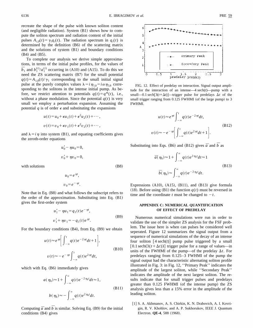
Numerous numerical simulations were run in ordervalidate the use of the simpler ZS analysis for the FSF prlem. The issue here is when can pulses be consideredseperated. Figure 12 summarizes the signal output frosequence of numerical simulations of the decay of an intefour soliton @4 sech(t)# pump pulse triggered by a [email protected] sech„3(t1Dt)…# trigger pulse for a range of values—iunits of the FWHMI of the pump—of the predelayDt. Forpredelays ranging from 0.125–3 FWHMI of the pump tsignal output had the characteristic alternating soliton proillustrated in Fig. 3: in Fig. 12, ‘‘Primary Peak’’ indicates thamplitude of the largest soliton, while ‘‘Secondary Peaindicates the amplitude of the next largest soliton. Thesults indicate that for small trigger pulses and predelgreater than 0.125 FWHMI~of the intense pump! the ZSanalysis gives less than a 15% error in the amplitude ofleading soliton.
@1# S. A. Akhmanov, A. S. Chirkin, K. N. Drabovich, A. I. Kovri-gin, R. V. Khohlov, and A. P. Sukhorukov, IEEE J. QuantuElectron.QE-4, 588 ~1968!.
FIG. 12. Effect of predelay on interaction. Signal output amptude for the interaction of an intense—4 sech(t)—pump with asmall—0.1 sech@3(t1Dt)#—trigger pulse for predelaysDt of thesmall trigger ranging from 0.125 FWHMI~of the large pump! to 3FWHMI.

n.
R
t.
pt
Op
an
. B
p.
u-
d.
n.
n,
PRE 59 6137THREE-WAVE INTERACTION SOLITONS IN OPTICAL . . .
@2# Y. Wang and R. Dragila, Phys. Rev. A41, 5645~1990!.@3# A. Stabinis, G. Valiulis, and E. A. Ibragimov, Opt. Commu
86, 301 ~1991!.@4# Y. Wang and B. Luther-Davies, Opt. Lett.17, 1459~1992!.@5# C. Y. Chien, G. Korn, J. S. Coe, J. Squier, G. Mourou, and
S. Craxton, Opt. Lett.20, 353 ~1994!.@6# J. D. V. Khaydarov, J. H. Andrews, and K. D. Singer, Op
Lett. 19, 831 ~1994!.@7# J. D. V. Khaydarov, J. H. Andrews, and K. D. Singer, J. O
Soc. Am. B12, 2199~1995!.@8# A. Umbrasas, J. C. Diels, J. Jacob, and A. Piskarskas,
Lett. 19, 1753~1994!.@9# S. Fournier, R. Lopez-Martens, C. Le Blank, E. Baubeau,
F. Salin, Opt. Lett.23, 627 ~1998!.@10# E. Ibragimov and A. Struthers, Opt. Lett.21, 1582~1996!.@11# E. Ibragimov and A. Struthers, J. Opt. Soc. Am. B14, 1472
~1997!.@12# V. E. Zakharov and S. V. Manakov, Zh. Eksp. Teor. Fiz.69,
1654 ~1975! @Sov. Phys. JETP42, 842 ~1975!#.@13# D. J. Kaup, Stud. Appl. Math.55, 9 ~1976!.@14# L. Torner, C. Menyuk, and G. Stegeman, J. Opt. Soc. Am
12, 889 ~1995!.@15# A. V. Buryak, Y. S. Kivshar, and S. Trillo, Opt. Lett.20, 1961
~1995!.@16# E. Ibragimov, J. Opt. Soc. Am. B15, 97 ~1998!.
.
.
t.
d
@17# D. J. Kaup, A. Reiman, and A. Bers, Rev. Mod. Phys.51, 275~1979!.
@18# Yu. N. Karamzin and A. P. Sukhorukov, Pis’ma Zh. EksTeor. Fiz.20, 734 ~1974! @JETP Lett.20, 339 ~1974!#.
@19# E. Ibragimov, J. D. Khaydarov, K. D. Singer, and Allan Strthers, inConference on Lasers and Electro-Optics, Vol. 11 ofOSA Technical Digest Series~Optical Society of America,Washington, DC, 1997!, pp. 200 and 201.
@20# M. J. Ablowitz and P. A. Clarkson,Solitons, Nonlinear Evo-lution Equations and Inverse Scattering~Cambridge Univer-sity Press, Cambridge, 1991!.
@21# D. J. Kaup, Phys. Rev. A16, 704 ~1977!.@22# J. W. Miles, SIAM ~Soc. Ind. Appl. Math.! J. Appl. Math.41,
2 ~1981!; 41, 227 ~1981!.@23# M. J. Ablowitz, D. J. Kaup, A. C. Newell, and H. Segur, Stu
Appl. Math. 53, 249 ~1974!.@24# H. A. Haus and M. N. Islam, IEEE J. Quantum Electron.QE-
21, 1172~1985!.@25# E. Ibragimov, A. Struthers, and D. J. Kaup, Opt. Commu
152, 101 ~1998!.@26# V. G. Dmitriev, G. G. Gurzadyan, and D. N. Nikogosya
Handbook of Nonlinear Optical Crystals~Springer-Verlag,Berlin, 1997!.
@27# S. D. Butterworth, L. Lefort, and D. C. Hanna~private com-munication!.