three topics in weather index insurance
TRANSCRIPT

THREE TOPICS IN WEATHER INDEX INSURANCE
A Thesis
Presented to the Faculty of the Graduate School
of Cornell University
In Partial Fulfillment of the Requirements for the Degree of
Master of Science
by
Michael Theodore Norton January 2009

© 2009 Michael Theodore Norton

ABSTRACT This paper presents three papers on the topic of weather index insurance, the
practice of mitigating risk according to objective measurements of weather conditions.
The topic has a simple premise, but the implementation is anything but. The
weather/crop yield relationship, and therefore risk, is not a straightforward function,
and weather observations seldom align themselves for easy analysis. Being a
relatively new technology, there are of course problems with implementation and rich
opportunities for research and analysis.
The first topic is to present the internet site that enabled access to the weather
data. It is groundbreaking and among the first of its kind. The second topic regards
plant disease risks when faced with risks in combination, specifically regards to heat
and drought risk occurring simultaneously, and the last topic is an algorithmic
approach to the problem of geographical basis risk.

iii
BIOGRAPHICAL SKETCH Michael Norton was born on September 16, 1978 in Austin, Texas to James F.
and Lynne L. Norton. He has an older brother, James, and a younger sister, Lesley.
Early life involved much moving and resettlement, living with his family in
Texas, California, and Delaware before settling in Langhorne, PA in 1987, from
whence he graduated from Neshaminy High School in 1995.
After a postgraduate year at The Peddie School in Hightstown, NJ, Michael
matriculated into Carnegie Mellon University in Pittsburgh, PA. Majoring in
Information and Decision Systems, Michael graduated from CMU in December of
2000.
Michael worked for a year at a subsidiary of Siemens in Malvern, PA, and
afterwards joined the Peace Corps. As a Peace Corps Volunteer in Malawi, Michael
taught math, history, and life skills at a secondary school for over two years. Upon
completion of service, Michael worked at the Population Studies Center of the
University of Pennsylvania on a social research project based in Malawi.
Michael began his studies at Cornell University in the fall of 2006.

iv
To my parents

v
ACKNOWLEDGEMENTS I am indebted to many people for their kindness and support, for without them
this thesis could not have been written.
First thanks goes to my advisory committee, Professors Calum Turvey and
Vicki Bogan, for their help and guidance in the conception of this paper.
Thank you to my parents, brother, and sister for their encouragement and
positive attitude. Everything that I’m able to accomplish is a direct result of their
support and guidance.
My friends in Ithaca, foremost Rachel Duncan for introducing me to makeover
TV shows, Leslie Verteramo for being a great guy to share an apartment with and
useful sounding board for my wildest ideas, Jacklyn Kropp for veteran advice and the
occasional drinking sojourn, John Taber for watching my cat for so long, Matt and
Jonica Leroux for being absolutely indispensable, and my officemates in Warren B37
for making me take out my earbuds and laugh every once in a while.
Big thanks to Linda Morehouse and the AEM staff for their unwavering
support from the time I submitted my application until the thesis defense. You guys
help more than you know.
Professors David Just, Antonio Bento, Jon Conrad, Loren Tauer, and Jeffrey
Prince: Thanks for making the AEM department such a worthwhile place to learn and
grow.

vi
TABLE OF CONTENTS Biographical Sketch .................................................................................................. iii Acknowledgements .................................................................................................... v Table Of Contents ..................................................................................................... vi List Of Figures .......................................................................................................... ix List Of Tables ........................................................................................................... xi List Of Abbreviations............................................................................................... xii List Of Symbols ...................................................................................................... xiii Chapter 1 - Introduction ............................................................................................. 1
The History of Weather Index Insurance............................................................... 1 Objectives ............................................................................................................ 3 Internet Tool......................................................................................................... 4 Joint Risk ............................................................................................................. 6 Geographic Basis Risk.......................................................................................... 6 Organization......................................................................................................... 9
Chapter 2 – Conceptual Issues In Weather Index Insurance ...................................... 10 Contract Design – Temperature Contracts........................................................... 13 Contract Design – Precipitation Contracts........................................................... 15 Payout Options ................................................................................................... 16 Commercial Purveyors ....................................................................................... 16 Adjusting the Specific Event Paradigm for Joint Risk Events ............................. 18
Chapter 3 - An Internet Based Tool for Weather Risk Management.......................... 19 Introduction........................................................................................................ 19 Economics and Weather Risk ............................................................................. 21 Frequency, Duration and Intensity of Specific Weather Events ........................... 25 Assessing Weather Risk and Weather Risk Insurance with Weather Wizard ....... 28 Heat Insurance.................................................................................................... 28 Precipitation Insurance ....................................................................................... 32 Summary............................................................................................................ 35
Chapter 4 - The Measurement and Insurability of Plant Disease Risks...................... 38 Insurability ......................................................................................................... 40 Karnal Bunt ........................................................................................................ 41 Silk cut (And The Need For Clarity) ................................................................... 44 Stewart’s disease ................................................................................................ 47 Conclusions........................................................................................................ 49
Chapter 5 – Weather Index Insurance and the Geographic Variability of Risk .......... 51 Defining the geographic area .............................................................................. 53 The Regression Equation .................................................................................... 56 Defining the Risk Events .................................................................................... 57 Regression Results ............................................................................................. 60 Improving the Fit ................................................................................................ 62 Out of Sample Predictions .................................................................................. 64 Summary............................................................................................................ 65
Chapter 6 – Conclusions........................................................................................... 67

vii
Future Research.................................................................................................. 68 Chapter 7 - Technical Specifications ........................................................................ 69
Software Vendors............................................................................................... 69 Data Summary.................................................................................................... 69
Appendix ................................................................................................................. 71 Appendix A – Weather Wizard Screen Shots...................................................... 71 Appendix B – Site Map for Weather Wizard....................................................... 76 Appendix C – State by State Data Summary ....................................................... 77 Appendix D – Code Samples .............................................................................. 79
Sample 1: Dat a Cleaning Algorithm............................................................. 79 Sample 2: Degree Day payout algorithm....................................................... 81 Sample 3: Multiple Event Contract algorithm ............................................... 81 Sample 4 : Cumulative Rainfall Payout algorithm......................................... 82
Bibliography ............................................................................................................ 84

viii
LIST OF FIGURES Figure 1: Daily maximum temperature observations for Ithaca, NY and three
closest weather stations for June-August, 1998. .................................................... 7 Figure 2: Daily temperature observations censored to display potential risk
events. .................................................................................................................. 8 Figure 3: Daily maximum temperature observations for two year period (Jan 1st
2000 – Dec 31st 2001) at Ithaca, NY station (with confidence intervals.)........... 10 Figure 4: Daily precipitation observations for two year period (Jan 1st 2000 –
Dec 31st 2001) at Ithaca, NY (with confidence intervals.) .................................. 11 Figure 5: Payoff schedule for precipitation risk event (from Shirley 2008) ............... 12 Figure 6: Sites in Iowa selected for study ................................................................. 47 Figure 7: Schedule of payouts for heat risk event...................................................... 58 Figure 8: Schedule of payouts for drought risk event ................................................ 59 Figure 9: Weather Wizard Main Screen.................................................................... 71 Figure 10: Date Selection Screen for Specific Event Risk ......................................... 72 Figure 11: Temperature Insurance Worksheet........................................................... 73 Figure 12: Temperature Insurance Worksheet illustrating excess heat risk ................ 74 Figure 13: Precipitation Insurance Worksheet........................................................... 75 Figure 14: Flow Chart for Weather Wizard............................................................... 76

ix
LIST OF TABLES Table 1: Historical Degree-Day Comparison for Ardmore, OK and Ithaca, NY ........ 29 Table 2: Degree-Day Heat Insurance Premiums based on 85° F Degree-Days
($1,000/degree) .................................................................................................. 30 Table 3: Multiple Event Heat-Wave Frequencies...................................................... 31 Table 4: Seasonal Cumulative Precipitation Insurance Premiums ............................. 33 Table 5: Multiple Event Cumulative Rainfall Insurance ($1,000 lump sum or
$1,000/inch) ....................................................................................................... 34 Table 6: (After Workneh et al 2008) ......................................................................... 42 Table 7: Frequency of high risk years for Karnal bunt in Olney and San Saba, TX ... 43 Table 8: Estimated insurance premiums for Olney and San Saba, TX ....................... 43 Table 9: Prevailing weather conditions for Corpus Christi, TX ................................. 45 Table 10: Frequency of high risk years at selected sites in Iowa................................ 49 Table 11: Estimated premiums for different breeds of corn....................................... 50 Table 12: Correlation of average of nearby stations of cumulative weather indexes .. 53 Table 13: Number of comparisons in Ithaca, NY for a given number of miles .......... 55 Table 14: Mean CDD (85° F) at each location .......................................................... 60 Table 15: Regression results for heat risk event ........................................................ 61 Table 16: Regression results for precipitation risk event ........................................... 62 Table 17: Results of transformations in the regression equation................................ 65 Table 18: Out-of-sample predictions......................................................................... 65
x
LIST OF ABBREVIATIONS APHIS – Animal and Plant Health Inspection Service (USDA)
CDD – Cooling Degree Days
GDD – Growing Degree Days
HDD – Heating Degree Days
NOAA – National Oceanic and Atmospheric Administration
OTC – Over the counter
SQL – Structured Query Language
USDA – United States Department of Agriculture
WRMA – Weather Risk Management Association
xi
LIST OF SYMBOLS Chapter 3:
x - an ordinary input (e.g fertilizer)
iα - random coefficients of the production function
ω - a specific weather event
H - stochastic household production function
- a weather/currency converter
Chapter 4:
p - the price per bushel of the crop in question
Y – normal yield
Y* - yield under stress
f (R,T,t): The frequency of a given weather event with respect to rainfall (R),
temperature (T), and time (t).
g(Θ): The probability of infection given favorable weather conditions.
Chapter 5:
Px – payout at station x
φ - distance between the two stations
αx - the altitude at each station,
ωx - the latitude at each station, and
λx - the absolute value of the longitude of each station

1
Chapter 1 - Introduction
This document is the culmination of two years of work on the topic of weather
index insurance, the practice of mitigating risk according to objective measurements
of weather conditions. The topic has a simple premise, but the implementation is
anything but. The weather/crop yield relationship, and therefore risk, is not a
straightforward function, and weather observations seldom align themselves for easy
analysis. Being a relatively new technology, there are of course problems with
implementation and rich opportunities for research and analysis.
Although there is an established market for weather derivatives on the Chicago
Mercantile Exchange (CME) for hedging weather-based risk, the products might be
considered to be more useful for industries like energy which primarily operate in the
cities in which the indexes are collated and have a more definitive relationship to
marginal gradations in temperature. It is still not understood how to define what
weather conditions create risk for agricultural producers and how precisely to model
those risk conditions at diverse locations, problems that will need to be overcome
before widespread adoption of weather index insurance can commence. What follows
is a series of three papers, prepared or intended for publication, that attempt to
ameliorate those problems.
The History of Weather Index Insurance
The energy industry has long been observed to be sensitive to variations in
weather conditions. Energy suppliers will prosper in a cold winter through a high
volume of energy sold, but is stifled in an abnormally temperate winter. The
benchmark is generally considered to be 65° F, a temperature above which people

2
demand electricity to cool buildings and below which demand energy (coal, natural
gas, electricity) for heating purposes. These revenue streams are highly variable and
highly dependent on the severity of a season. Traditionally, this wasn’t a problem
because suppliers faced no competition in a market and received government price
guarantees. With the advent of deregulated energy markets in the 1990s, energy firms
found the need to hedge against weather risk, and thus the weather derivatives market
was born. An early pioneer in the weather derivatives market was Enron, through its
Enron Online unit.
In its current form, the market at the CME will allow an energy supplier to
purchase a non-asset based futures contract pegged to a weather index. For example,
an energy supplier may wish to write an option contract that will pay off if a summer
is sufficiently hot, reasoning that in such conditions revenues will be healthy enough
so that they will happily cover the cost of the option payout. If the summer is cool, the
energy company would generate less revenue from the sale of electricity, but will
pocket the premium for writing the contract and thus smooth their revenue stream.
The CME now includes 645 weather products for 35 cities worldwide, as well as
hurricane indices for the East and Gulf Coasts. In addition to the futures and options
traded on the CME, third-party vendors also sell customizable over-the-counter
contracts for virtually any combination of temperature event imaginable. As of 2005,
Turvey reports that 4000 transactions occurred that were worth $8 bn (Lyon 2004).
Organizations like the Weather Risk Management Association (WRMA) now
exist which bring together principals from the meteorology, insurance and finance
industries to accomplish such goals as establishing standards for credit and expanding
the weather market geographically. The concepts developed for the energy industry
also apply to other fields, and much of the current research involves applying the

3
successful strategies developed for the energy industry for other weather-sensitive
industries.
The successful development of methods for pricing weather index insurance
contracts will likely have profound impacts on developing countries, which are highly
dependent on agriculture. The sheer number of smallholder farms in these countries
precludes the dissemination of traditional adjustment-based insurance policies even
though impoverished farmers bear the full brunt of climatic variability. A successful
implementation of a weather index insurance program would likely have profound
implications for improving the livelihood of farmers in these countries by preventing
them from falling into a “poverty trap” when faced with crop losses due to adverse
weather conditions. (Skees 2008)
Objectives
The purpose of this research is to refine and develop methods for pricing
weather index insurance by taking observations of a stochastic process. The markets
described above for the CME and any over-the-counter (OTC) represent the
foundations of weather index insurance or any weather derivative product. However,
they require strict assumptions. First, risk events are only considered as separate
entities, even though stress events often have more profound negative impacts on
crops when happening simultaneously. Often, calculating risk on single events is
incomplete, especially in regard to plant pathogens like fungi, molds, and insects that
require specific meteorological criteria for their presence. Developing a method for
pricing insurance for joint probabilities is necessary for the successful wide scale
adoption of weather index insurance.
Second, these products price their products at a single location and assume that
weather patterns at that fixed location are adequate to describe weather conditions at
4
the site of the insured event. This is not always the case and an understanding of
conditions at the insured location is often required. The difference in risk profile
between the measured location and the insured location is known as geographic basis
risk, and it is a problem which to this date has not been adequately resolved.
Third, the process to model single, joint, or geographic risk profiles is
computationally intense and requires the manipulation of large amounts of weather
data. The computational intensity is unto itself a problem and the pursuit of an
algorithmic, generally applicable, and flexible tool to assist in computation and
analyses is unto itself a worthwhile pursuit. Thus, in order to design and price weather
insurance for multiple or single events with independent or joint risks, while taking
into consideration basis risk, a major contribution of this research is the design and
web placement of a computer program which we refer to as Weather Wizard.
This thesis extends the existing literature in three ways: by introducing an
interactive web tool for further analysis, by providing a measure of joint weather
events in regard to pest risks, and beginning analysis of geographic spread of risk.
Internet Tool
The first contribution of this thesis is the development of an internet tool to
facilitate analysis of weather observations. Given the virtually limitless number of
possibilities for contract design, a flexible and accessible tool was needed to facilitate
understanding of the nuances thereof. Thus, through a grant from the Risk
Management Agency (RMA) of the U.S. Department of Agriculture (USDA), the
Weather Wizard website was born.
Weather Wizard contains data from the (NOAA) for over 25,000 stations
across the U.S., with observations stretching back more than 100 years in some cases.

5
It contains information on four different weather indexes – rainfall, high temperatures,
low temperatures, and mean temperatures.
The advantage of offering the functions of Weather Wizard in a web format is
the absolute transparency it offers. Although not allowed to display individual
weather observations, it does allow any argument made in an academic context to be
instantly verified by anyone with an internet connection. All of the functionality
presented in this thesis has been programmed into Weather Wizard, and it is possible
to retrace the exact steps taken in analysis.
Furthermore, Weather Wizard not only allows accessibility but allows the user
absolute flexibility to select the parameters for analysis. Too often weather
management tools – like the MSI Guaranteed Weather website – only offer
observations from the most recent years (starting 1950) and in certain weather stations.
Some of the major variations we have seen occurred in periods like the Dust Bowl of
the 1930s, and to censor data before a certain date is to remove a major source of
information. Likewise, Weather Wizard allows for the selection of any weather
station for which the NOAA provides data, no matter how few years of data exist (a
decision that will have important implications for the discussion on geographic basis
risk.)
Although Weather Wizard has until now been used mainly by researchers in-
house at Cornell University, it has the potential to be used by not only researchers at
outside institutions but the principals in the contract themselves. Weather Wizard is
not intended to be a commercial enterprise, but the concepts used are of undoubted
interest to the insurance and financial industries.

6
Joint Risk
As valuable as a weather index might be, it does not include all of the
potentially valuable information that we may have about growing conditions at a
specific station. Any attempt to mitigate local basis risk by examining the
weather/crop yield relationship is necessarily incomplete without considering the
interaction between heat and precipitation stress events, as the presence of one often
compounds the negative effects to crop yields. Indeed, Mittler (2006) states that
plants subject to a combination of weather risks will have a “molecular and metabolic
response … [that] is unique and cannot be extrapolated from the response of plants to
each of these different stresses applied individually.”
In addition, risk criteria for weather index insurance are often ill-defined and
therefore subject to imperfect hedge ratios. By taking our risk parameters directly
from the scientific literature and basing our yield loss estimates on crop damage rather
than a production function we may avoid some of the more serious problems with
weather index insurance.
Geographic Basis Risk
Berg and Schmitz (2008) state that “geographical basis risk could probably be
reduced substantially by utilizing the information of several surrounding weather
stations instead of only the nearest one.” With the wealth of data available via
Weather Wizard, it is possible to begin analysis of geographic basis risk.
Currently, farmers in rural locations would be expected to purchase weather
index insurance indexed to a certain weather station in close proximity to their farm.
This station would need to have similar weather patterns and be well-established with
many years of data to accurately price historical frequencies. Unfortunately, the

7
choice is not always clear as to which station would properly mimic the risk
conditions present at the farm, or if a distant location will even be able to properly
mimic risk at the farm site in question.
50
55
60
65
70
75
80
85
90
95
100
6/1/
1998
6/8/
1998
6/15
/199
8
6/22
/199
8
6/29
/199
8
7/6/
1998
7/13
/199
8
7/20
/199
8
7/27
/199
8
8/3/
1998
8/10
/199
8
8/17
/199
8
8/24
/199
8
8/31
/199
8
Tem
pera
ture
IthacaAuroraCortlandSpencer
Figure 1: Daily maximum temperature observations for Ithaca, NY and three closest
weather stations for June-August, 1998.
For illustration, Figure 1and Figure 2 use the exact same data on different
scales. Figure 1 shows daily temperatures moving in virtual lockstep for Ithaca, NY
and the three closest stations from the period June 1st – August 31st. However, when
we censor that data to consider a risk event (temperatures in excess of 85° F), the
distribution becomes very different, and the differential in risk events become more
apparent. A farmer in close proximity to the Cortland weather station received far
more exposure to high temperatures than a farmer in Ithaca, revealing an ambiguity
for any farmers located in between the two stations (which are 20 miles apart.) But

8
this example is just in a small geographic area for a single growing season, and an
effort needs to be made to look at the problem of geographic basis risk in a more
systematic fashion.
85
86
87
88
89
90
91
92
93
94
1 4 7 10 13 16 19 22 25 28 31 34 37 40 43 46 49 52 55 58 61 64 67 70 73 76 79 82 85 88 91
Tem
pera
ture
IthacaAuroraCortlandSpencer
Figure 2: Daily temperature observations censored to display potential risk events.
Organization
Chapter 2 provides a background of conceptual issues in weather index
insurance, provides a technical definition for weather index insurance contracts, and
outlines the current state of research.
A full treatment of the Weather Wizard website is presented in Chapter 3,
which was published in the April 2008 issue of the Agricultural and Resource
Economics Review.

9
Chapter 4 considers the simultaneous occurrence of risk events with regard to
specific plant disease risks: Karnal bunt of wheat, Stewart’s disease and silk cut in
corn. In each case, risk parameters are derived from the plant disease literature and
adapted to price insurance premiums based on the historical incidence of weather
patterns and disease infection rates.
Our task in Chapter 5 was to uncover a systematic relationship in the spatial
relationships between stations and begin to price contracts for locations where no
weather station exists, and whether or not risk premiums can be correlated to simple
geographic variables.
Finally, a summary of major points and concepts is presented with conclusions
in Chapter 6.
For reference, two appendixes are included after Chapter 7, one with code
samples of Weather Wizard, and one with technical specifications used in the creation
of the website.
10
Chapter 2 – Conceptual Issues In Weather Index Insurance
Although we refer to weather index insurance as a single concept, to do so
glosses over the complexity therein. There are a great many options for writing
contracts based on a few simple weather indexes, and that is in part because of the
vastly different natures of the indexes. The raw data for temperatures and
precipitation is distributed in very different fashions and any contract written must do
so within the parameters of the variability of the index while also keeping in mind the
specific risk requirements of the insuree.
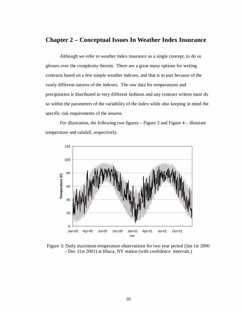
For illustration, the following two figures – Figure 3 and Figure 4 – illustrate
temperature and rainfall, respectively.
0
20
40
60
80
100
120
Jan-00 Apr-00 Jul-00 Oct-00 Jan-01 Apr-01 Jul-01 Oct-01Date
Tem
pera
ture
(F)
Figure 3: Daily maximum temperature observations for two year period (Jan 1st 2000
– Dec 31st 2001) at Ithaca, NY station (with confidence intervals.)

11
-2
-1
0
1
2
3
4
5
1/1/98 4/1/98 7/1/98 10/1/98 1/1/99 4/1/99 7/1/99 10/1/99
Prec
ipita
tion
(in.)
Figure 4: Daily precipitation observations for two year period (Jan 1st 2000 – Dec 31st
2001) at Ithaca, NY (with confidence intervals.)
Daily maximum temperature observations are cyclical throughout the year,
peaking in July and reaching a nadir in January and February. The gray confidence
intervals do not reflect a constant variance as the variance in summer temperatures is
much less than winter, but is somewhat contiguous. It may differ from season to
season but does not contain any obvious spikes during which individual days are
considerably more variable than others.
Rainfall measurements, by contrast, reveal a fairly constant mean throughout
the year. The variability decreases in the winter months, which is probably due to the
fact that precipitation in Ithaca will often instead be counted in the snowfall data for
those months. Certainly we can say that the variability is not as contiguous as
individual days will often have abnormal levels of variance, probably due to the
effects of a few large observations. (We can see one here in the second year of study –
Ithaca recorded 3.9” of precipitation on September 25th, 2001) The presence of rain is

12
episodic and unpredictably random in its invocation, and the variability includes the
zero value in all instances because of the large number of observations in which there
was no daily rainfall.
We want to properly design insurance products to cover a rare event. The
rarity itself is variable, whether it be a 1 in 10 year event or a 1 in 20 year event, all
monies paid out by the policy must also be paid in. A properly designed insurance
product will not only provide an accurate measure of risk but also consider the
requirements of the policy holder. This becomes difficult when we consider all of the
potential parameters in a weather contract, frequency, intensity, location, and duration.
It is the variable distribution of these risk events that we want to insure against,
and they may be designed in several ways. One example comes from the World Bank
project underway in Malawi, which offers drought insurance to subsistence farmers.
For rainfall amounts under a certain threshold (120 mm), the policy pays a variable
amount until a lower threshold (50 mm) of rainfall is reached, at which point it is
considered that the crop was a total loss and further compensation in unnecessary.
Figure 5: Payoff schedule for precipitation risk event (from Shirley 2008)
13
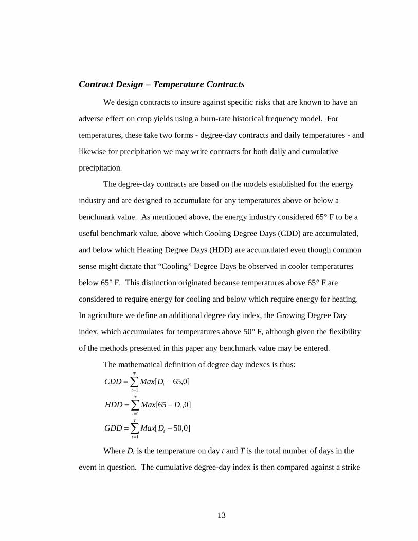
Contract Design – Temperature Contracts
We design contracts to insure against specific risks that are known to have an
adverse effect on crop yields using a burn-rate historical frequency model. For
temperatures, these take two forms - degree-day contracts and daily temperatures - and
likewise for precipitation we may write contracts for both daily and cumulative
precipitation.
The degree-day contracts are based on the models established for the energy
industry and are designed to accumulate for any temperatures above or below a
benchmark value. As mentioned above, the energy industry considered 65° F to be a
useful benchmark value, above which Cooling Degree Days (CDD) are accumulated,
and below which Heating Degree Days (HDD) are accumulated even though common
sense might dictate that “Cooling” Degree Days be observed in cooler temperatures
below 65° F. This distinction originated because temperatures above 65° F are
considered to require energy for cooling and below which require energy for heating.
In agriculture we define an additional degree day index, the Growing Degree Day
index, which accumulates for temperatures above 50° F, although given the flexibility
of the methods presented in this paper any benchmark value may be entered.
The mathematical definition of degree day indexes is thus:
T
ttDMaxCDD
1]0,65[
T
ttDMaxHDD
1]0,65[
T
ttDMaxGDD
1]0,50[
Where Dt is the temperature on day t and T is the total number of days in the
event in question. The cumulative degree-day index is then compared against a strike

14
value, which operates similar to an option contract as both calls and puts may be
written.
The generalized payout functions are similar and differ only in terms of the
benchmark value and direction of accumulation. The payout function for CDD is
given by:
dDDDDfDDMaxCDDPayout T )()0,65(][
Where is the payout multiplication parameter and f(DD) is the density
function of the statistical distribution of degree days. (Full discussion on is in the
Payout Options section.) For f(DD) we may insert several different types of function.
For this thesis, we use a burn rate analysis based on historical frequencies, but other
researchers have used a log-normal distribution (Cao and Wei 1999) or ().
For historical burn-rate analysis we may rewrite this payout function not as an
integral but as two nested addition functions.
N
n
T
tntDMax
NCDDPayout
1 1, ]0,65[1][
Where N is the number of years for which we have data, and Dt,n is the daily
temperature value for day t in year n. This will give us the average number of degree
days for the given date and year range at a particular station.
For daily temperature contracts, instead of an accumulation of degree days we
define a specific event risk each period for which the temperature observation is above
or below a certain threshold. For example, we might consider a heat risk event as
temperatures above X degrees for Y days, where X is a relatively high temperature
like 85° F and Y is a period which is determined to result in crop damage for heat. We
calculate the number of non-overlapping events within the date range for which these
criteria are met and multiply the payout amount by that number, up until a maximum

15
set by the user. The final payout is determined by the average number of observed
risk events across the entire range of years.
For example, if we are looking at 14-day heat waves, only two events are
possible in the month of June, since the events are non-overlapping. Each year will
have either 0, 1, or 2 observed events, and the average of this number will determine
the actuarially fair premium when multiplied by the payout parameter .
Contract Design – Precipitation Contracts
Daily rainfall contracts are identical to the daily temperature payouts in that
specific events are defined by a comparison of daily values. The difference is one of
scale, in that the index is not in degrees but inches.
For example, a drought might not be defined as a period without any
precipitation at all, but under a small threshold amount for each day. Using a daily
rainfall contract, we might define a drought as X consecutive days with rainfall below
Y inches, where Y is a value like 0.05” and X is a value assigned to reflect the number
of days beyond which crops would suffer from an absence of moisture.
Cumulative rainfall contracts share some similarities with the degree-day
contracts, in that they are both accumulating values across a date range. However,
cumulative rainfall differs in that multiple events may be selected, just as in the daily-
type contracts, whereas the degree-day contracts are by default across the entire date
range. If the insuree desired a contract in the cumulative rainfall mode similar to the
daily rainfall mentioned previously, the X entered would be the total rainfall across a
date range, regardless of the daily values. Just as in the daily measurements, these
events are non-overlapping and only a certain number could happen in any given year.
For example, we might define a drought as less than X” total across Y days.
16
Payout Options
The contract options allow for some flexibility in payout amounts. For the
daily temperature and rainfall contracts, the payoff is calculated for each observed
event, and some differentiation in the pricing is achieved by allowing for multiple
events. In other words, the severity of a year can be assessed by the number of risk
events occurring and insurance premiums can be adjusted accordingly.
However, for the degree-day, and to a lesser extent the cumulative rainfall, we
cannot use this method because the index accumulates across the entire date range. To
price the premium using this method would result in a series of binary payments in
which the criteria was either fulfilled or wasn’t. The solution to this is to offer a
“Unit” payout which pays out based on the severity of the season in question. For
severe results
For example, let’s say we set the strike value in a CDD contract to be 100, but
observe 150 degree days in a given period. Under the “Lump Sum” option, the payout
would be a straight sum, but for the “Unit” payout it would be multiplied by 150/100
= 1.5 to arrive at the final value. In this way we may adjust the payout amounts to
reflect the severity of a season. An illustration of this may be found in Figure 5 above,
which also has a ceiling above which the payout does not vary, as it is assumed that
any rainfall below 50 mm will result in total crop failure.
Commercial Purveyors
For real-world examples, MSI Guaranteed Weather LLC
(http://www.guaranteedweather.com/), a commercial purveyor of weather index
insurance, provides functionality similar to Weather Wizard, but offers many
examples for heat and precipitation products for industries including agriculture,
construction, energy, health, and leisure. Some sample weather products include:

17
Insurance for barley growers for excessive precipitation with payoffs
for each three consecutive days with total precipitation >= 0.35 inches,
for up to nine events.
A policy designed to insure against excessively cold days which
interrupt construction projects. Payoff of $50,000 for each day in
which the low temperature is <= 10° F in excess of 10 days in any
given year.
A policy for a theme park that wanted to insure against lost revenue for
rainy days. For any day in excess of 8 days in which the rainfall was
more than 3mm, the park was paid $25,000.
If risk conditions may be precisely defined, it is very easy to price these
insurance contracts from the data, but therein lies the difficulty, as it may not always
be said with certainty that the observed historical frequency of any given event will
allow for accurate pricing of an insurance policy.
Indeed, the underlying weather index is not a simple reflection of downside
risk. The difference between the payoff of the insurance contract and the underlying
risk is known as basis risk, and is a fundamental problem. Weather index insurance
substitutes the problems of adverse selection and moral hazard with the problem of
basis risk, and any effort to implement weather index insurance is an effort to
systematically reduce basis risk.
Basis risk may take two basic forms in the context of weather index insurance.
First, “local” basis risk refers to the phenomenon by which observed weather variables
do not correspond strongly with yield losses. We must recognize that weather is
undoubtedly a factor in crop production, but must be considered simultaneously with

18
other, often undetectable factors. Furthermore, stations with a dearth of useable data
will experience difficulties in accurate pricing.
The second type of basis risk is referred to as “geographical” basis risk, and
refers to the spatial relationships of risk in a geographic area and the variance
introduced at increasing distances from locations where the weather observations are
known quantities.
Adjusting the Specific Event Paradigm for Joint Risk Events
As valuable as the study of single event risks is, we also want to consider risks
that happen simultaneously, especially if they have effects above and beyond those
caused by their solitary presence – a classic example of a joint risk scenario is a
combined heat/drought event. It is easy to tabulate the number of years for each
individual risk event (e.g. both heat and drought) and arrive at two separate premiums,
but to do so would ignore the years with combined effects.
To calculate the joint risk premium for a given event, the risk event is only
considered to be present in years in which all risk events occurred, regardless of the
number of times they occurred. This is because it is impossible, as a general rule, to
compare risk events of different types without further inquiry into the nature of joint
risk. This is especially true when considering that the date ranges are variable for each
event.
Weather Wizard has been programmed to do just this, and will tabulate the risk
but the final output is a percentage of the years in which all risk conditions were
present. It is that percentage that we use to calculate the insurance premiums in
Chapter 4.

19
Chapter 3 - An Internet Based Tool for Weather Risk Management
Introduction
The pricing of weather insurance, and more generally the enumeration of
weather risk, is not an easy task. Data are not so easily accessible, and assessing the
data in terms of all of the possibilities of risk is burdensome (Campbell and Diebold
2003, Changnon and Changnon 1990). Furthermore the numbers of possibilities are
virtually endless, and what might be an insurable weather risk at one location may not
be insurable at another. It is for this reason that academic research has focused so
heavily on the general rules of probability that govern loss and weather
insurance/derivative premiums rather than making broad generalized statements about
application (Turvey 2005).
There are two gaps in the literature. The first is rudimentary. The literature on
weather risk management as cited above focuses more on insurability than on how
weather interacts with agricultural production and farm households as a source of risk.
The idea that weather and crop yields represent covariate risks is taken as given and
the effects of climate and weather variance on crop production has long been
understood (Bardsley, Abey, and Davenport, 1984; Changnon, 2005 ; Huff and Neill,
1982; Runge, 1968). A more complete understanding of how covariate risks evolve in
a production system, even at the conceptual level, can provide invaluable insights to
the practitioner and theorist. In this paper we present such a model. It is not a precise
model, nor are we in a position to empirically validate the model, but it does provide
the requisite insight to understanding covariate risk and how covariate risks interact
with farm livelihoods to create an insurable condition.

20
The second gap, and the focal point of this paper, is the measurement of
weather risk and the insurability of weather risk. Despite recent interest in weather
insurance, the idea of insuring weather risk as an alternative to crop insurance is not
new (several articles predating 2000 that made such propositions include Changnon
and Changnon, 1990; Gautman, Hazell, and Alderman, 1994; Quiggin, 1986; Patrick,
1998 ; Sakurai and Reardon, 1997). Since 2000, a variety of weather insurance
models, propositions, theorems, and structures have been proposed, but there is little
agreement on how weather risk should be defined or how weather insurance should be
priced [Alaton, Djehiche and Stillberger, 2002, Alderman and Haque, 2006, Cao and
Wei, 2004, Considine, (undated), Davis, 2001, Dischel, 2002, Geman, 1999, Jewson
and Brix, 2005, Leggio, and Lien, 2002, Muller and Grandi, 2000; Nelken, 1999,
Richards, Manfredo, and Sanders, 2004, Turvey 2001, 2005, Zeng, 2000].
Applications of weather insurance in North America, Europe and developing
economies are varied and include numerous important contributions to a range of
issues including agricultural production risk, food security, poverty alleviation,
irrigation insurance, intertemporal risks and so on (Alderman and Haque 2006, Hao
and Skees 2003, Hazell, Oram and Chaherli 2001, Hazell and Skees 2006, Hess,
Richter and Stoppa 2002, Lacoursiere 2002; Leiva and Skees 2005; Mafoua and
Turvey 2003, Martin, Barnett and Coble 2001, Muller and Grandi 2000, Skees, Hartell
and Hao 2006, Skees, Gober, Varangis et al 2001, Stoppa and Hess 2003, Turvey,
Weersink, and Chiang 2006, Vedenov and Barnett 2003, Veeramani, Maynard and
Skees 2004).
Part of the problem is that use of the term ‘weather risk’ is far too ubiquitous
and agricultural economists seeking agreement on a definition of weather risk will
ultimately be disappointed. As will be discussed presently, the term implicitly includes
considerations of frequency, intensity, and duration. The gap extends when one asks

21
“what risk?” and expands even further when one tries to determine, evaluate or
measure the risk. It is no easy task and perhaps too much of the academics’ energy is
used on measuring the risk rather than defining the risk and applying the risk. This is
at the core of this paper. In this paper we describe a web-based application program
called Weather Wizard (www.weatherwizard.us) that was developed along the lines of
Turvey (2001) for specific event temperature and precipitation risks and Turvey
(2005) for degree-day temperature risk. The program accesses heat and precipitation
data for all NOAA weather stations (currently available to 2001) in the United States
and can be used to investigate weather related risk and calculate insurance for virtually
all possible single and multiple specific events.
The main contribution of this research is the outreach tool itself. Weather
Wizard can be accessed by researchers, crop insurance specialists, educators and
practitioners. In a very short period of time measured in minutes rather than days or
weeks, the user can select any location, define a specific event, and enumerate that
risk. Furthermore, users can evaluate up to five joint precipitation and temperature
risks as well as basis risk for a specific weather event for all weather stations within 50
miles of a specific location.
The paper proceeds as follows. First, we provide a conceptual overview of
weather risk in the theory of production. Second, we focus on the meaning of “weather
risk” and then we describe in general terms the underlying philosophy of the computer
program and the meaning of specific event risk. In the Appendix, the program is
illustrated in terms of screen displays and application.
Economics and Weather Risk
The central focus of this paper is the presentation of a web-based computer
program designed for the measurement of weather risk. To motivate the need for such

22
a program, this section outlines the relationships between production economics,
weather risk and farm livelihoods to show how specific weather events interact as a
source of risk and how these risks can be mitigated using weather insurance. We make
two assumptions. First we assume that the specific weather event is treated as a
stochastic input into the production function and second, livelihood is measured in the
context of a whole farm or household production function. We do not assume a
stochastic production function that simply adds randomness to a deterministic
function. Rather, we assume that the weather event creates randomness in the
production coefficients themselves so that marginal productivity is endogenously
random. Keeping in mind that any production function will do, we start with a
classical form of production:
(1) 21 2 3,ω =α ω +α ω -α ωY x x x
where x is an ordinary input (e.g., fertilizer) , and iα are random
coefficients of the production function. If one were to assume that
ω ωi i i i is a function of some specific weather event ω defined over
some (known or unknown) probability distribution function that describes the specific
event risk, then the stochastic production function is
(2) 2 21 1 2 2 3 3 1 2 2,ω α +β α +β α +β ε ε εY x x x x x ,
with expected production being
(3) 2332211 )()()],(,[ xxxYE
Under the independence assumption, yield variance, conditional on weather
risk, is defined by
(4) 12 31 2 3
2 2 2 2 2 2 2 2 2 2 2 4ε ω ε ω εσ β σ σ β σ +σ β σ +σY x x .
In words, the standard errors of the production coefficients comprise two
influences. The first, we argue is the influence of weather risk, and the second is an
unrelated risk. It is of course assumed that if weather insurance is to be viable as a risk
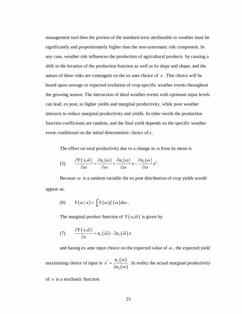
23
management tool then the portion of the standard error attributable to weather must be
significantly and proportionately higher than the non-systematic risk component. In
any case, weather risk influences the production of agricultural products by causing a
shift in the location of the production function as well as its slope and shape, and the
nature of these risks are contingent on the ex ante choice of x . This choice will be
based upon average or expected evolution of crop-specific weather events throughout
the growing season. The interaction of ideal weather events with optimum input levels
can lead, ex post, to higher yields and marginal productivity, while poor weather
interacts to reduce marginal productivity and yields. In other words the production
function coefficients are random, and the final yield depends on the specific weather
event conditional on the initial deterministic choice of x .
The effect on total productivity due to a change in from its mean is
(5) 1 1 1 2, α α αY xx x
.
Because is a random variable the ex post distribution of crop yields would
appear as:
(6) |l
uY x Y f d .
The marginal product function of ,Y x is given by
(7) 2 3
,α 2α
Y xx
x
and basing ex ante input choice on the expected value of , the expected yield
maximizing choice of input is
2*
3
α2α
x
. In reality the actual marginal productivity
of x is a stochastic function.

24
(8) 22 3, α α
2Y x
xx
,
which can also be expressed as a conditional marginal product function
(9) *
l*
u
|MPP |
Y xx f d
.
In other words, weather is not simply a passive actor in agricultural
productivity, but can change not even the total productivity by shifting the production
function up or down, but also the marginal productivity. Nor is it a simple distribution
about some level of expected yields, but a factor that can change the shape of the
production function throughout the range of x . The efficiency of production is also at
risk. Given a prior choice of x and no bounds on i , 2 ,0
Y xx
such that
ex post production relative to input choice can exhibit increasing, constant or
diminishing returns to scale, even though in the deterministic model, only diminishing
marginal productivity would be observed.
We now define a weather contingent livelihood function that can be thought of
as a stochastic household production function. Its general form is given by
(10) , ,u
lH Y h Y f d .
Weather risk enters the livelihood function in two ways. First, as discussed
above, agricultural productivity is affected directly by weather risk, but other aspects
of livelihood can also be affected. For example, if the farm is financially leveraged,
short on working capital or requires investment, liquidity shortfalls from adverse
weather events can have economic impacts beyond production. Thus the more flexible
form of weather risk management is not necessarily tied to agricultural productivity,

25
but household livelihood. From this we can extract the coverage for specific event
weather by extracting from H the value for that satisfies a minimal livelihood
level *H
, * -1H
. Therefore, a downside weather risk policy will be
established according to
(11) *E Max ,0 E Max ,0H H
,
where converts units of weather into units of currency. A convenient
measure is *
H
.
It is this interaction between production and farm household well-being that
motivates weather risk as an area of study and makes weather insurance useful.
However, the actual measurement of weather risk is not easily accomplished. The
characteristics of weather risk are discussed in the next section and the tool developed
to measure weather risk and weather risk insurance follows.
Frequency, Duration and Intensity of Specific Weather Events
The preceding discussion uses the term “weather risk” in a very general way. It
is in fact more complex than a simple definition of a random variable as described.
The intent above was to provide a conceptual basis for the measurement of risks that
follow. For purposes of this paper and the description of Weather Wizard, we will use
for determining the expectation of loss the working definition that a specific event risk
is uniquely defined at any location by the functional relationship between duration,
frequency, and intensity. Duration is a definition in time ranging from a day, week,
month, year or more or less. The model additionally uses the concept of multiple
events, which infers a second dimension of time. The first dimension therefore
measures the period over which the weather event is to be investigated while the
second dimension is a time frame within that period. For example, duration could be
measured by any non-overlapping 21 day period between June 1 and August 31. There

26
is a possibility of four non-overlapping events. If it were measured on a 7-day basis,
there could be as many as 12 non-overlapping events.
Frequency measures the probability scale defined in terms of the frequency
that the event occurs over the specified duration. Frequency here can be based on
historical fact (often referred to as the burn rate) or by a defined distribution (e.g., an
assumption of log normality).
Intensity is a measure of scale and refers to the quality or condition under
investigation and thus requires a point of reference from which quality can be
measured and a directional indicator by which condition can be measured. The former
will usually be measured by a quantitative criterion such as rainfall or temperature,
and the condition is normally defined by whether the actual quantity is above or below
the point of reference.
But the terms in their totality must remain flexible. For example a degree-day
derivative product is normally defined for a single event in which the event length
equals the period over which the product is being measured. Extreme heat or heat
waves regarded as a sequential number of days over which daily temperatures exceed
a criterion can be defined as multiple events. Likewise, precipitation events based on
daily or cumulative precipitation can be multiple or single events and so on.
Care must also be taken in establishing the criteria. Specificity is important.
For example we do not in any of our models facilitate insurance or risk management in
terms of averages because averages, unto themselves are meaningless. Specific events
as we have defined them are based wholly on the sequencing and timing of weather
patterns for which full information on the frequency, duration and intensity is
required.
The final element is loss value. Unlike crop insurance for which a measured
loss can be ascertained by the actual weight of crop harvested times a price, the loss

27
value from yield-independent weather risk is less obvious. By “yield-independent” we
mean that any payout from weather insurance is provided based on recognized
weather measurements at specific weather stations rather than yield loss. It is of course
assumed that there is some a priori recognition that the weather event will be highly
correlated with yield loss and that the loss value can be estimated or approximated so
that volumetric loss is approximated more or less. This might allow for some
speculation on the part of the insured but such speculation does not constitute moral
hazard or adverse selection as it is normally construed in the insurance literature, since
the premium calculated is actuarially consistent with the weather event. Nonetheless, it
serves little purpose to even consider specific events near the average since such
insurance will ultimately be expensive and largely uncorrelated with yield loss.
Rather, weather insurance should focus on events of the extreme for which, at least
within the realm of memoried probability, would most surely result in volumetric and
economic loss. For example, it makes little sense for an insured to select a contract
insuring against a heat wave based on daily high temperatures in excess of 75° F when
loss does not occur until temperatures exceed 90° F; or insuring against less than 1” of
cumulative rain over 7 days when it is known that the crop can withstand 21 days with
no or little rain.
On this basis we use two dollar-valued measurements. The first is a lump sum
or binary payout which simply pays an agreed sum if the event occurs (regardless of
intensity) and zero otherwise. The second is a unit payout, similar to options payouts
or crop insurance payments in which the payout for each event increases linearly with
intensity. The binary option is simple and convenient and is most applicable when the
event itself, rather than the intensity of the event is what causes risk. For example, it
matters not whether a frost event is measured at 31° F or 20° F, the damage is still
done, or if it rains less than 2” in 21 days, irrigation costs will still be incurred whether
28
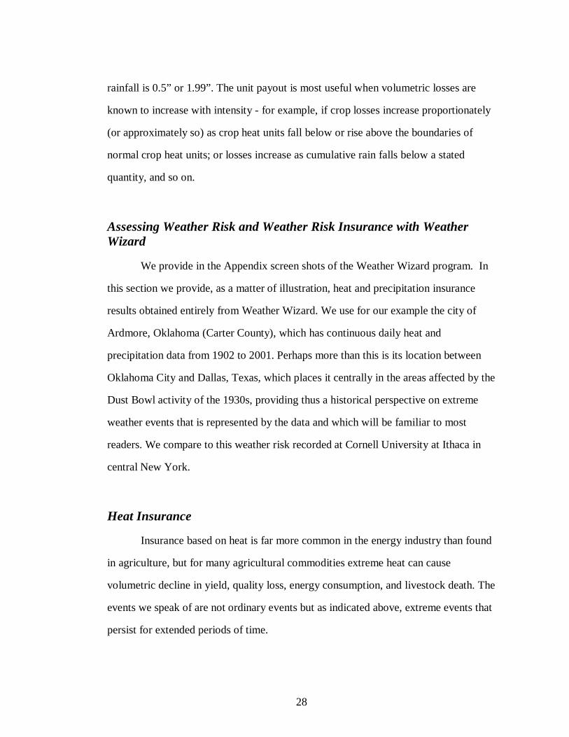
rainfall is 0.5” or 1.99”. The unit payout is most useful when volumetric losses are
known to increase with intensity - for example, if crop losses increase proportionately
(or approximately so) as crop heat units fall below or rise above the boundaries of
normal crop heat units; or losses increase as cumulative rain falls below a stated
quantity, and so on.
Assessing Weather Risk and Weather Risk Insurance with Weather Wizard
We provide in the Appendix screen shots of the Weather Wizard program. In
this section we provide, as a matter of illustration, heat and precipitation insurance
results obtained entirely from Weather Wizard. We use for our example the city of
Ardmore, Oklahoma (Carter County), which has continuous daily heat and
precipitation data from 1902 to 2001. Perhaps more than this is its location between
Oklahoma City and Dallas, Texas, which places it centrally in the areas affected by the
Dust Bowl activity of the 1930s, providing thus a historical perspective on extreme
weather events that is represented by the data and which will be familiar to most
readers. We compare to this weather risk recorded at Cornell University at Ithaca in
central New York.
Heat Insurance
Insurance based on heat is far more common in the energy industry than found
in agriculture, but for many agricultural commodities extreme heat can cause
volumetric decline in yield, quality loss, energy consumption, and livestock death. The
events we speak of are not ordinary events but as indicated above, extreme events that
persist for extended periods of time.

29
Table 1 provides a summary of degree-days for Ardmore and Ithaca. Recall
that degree-days in the energy industry are measured relative to 65° F and corn heat
units relative to 50° F, but this need not be viewed as a meaningful economic standard.
Heat stress in agriculture does not in most cases occur until temperatures are well in
excess of 80° F, so it makes little sense to include temperatures below the stress levels.
But stress must also be measured relative to climate. The degree-days measured in
Table 1 are obtained by adding together the difference between the (91) daily high
temperatures in excess of the degrees identified in the first column. The mean degree-
days are provided in column 2, the standard deviation across years in column 3, and
the historical maximum and minimums in columns 4 and 5. For the same temperature
measures the degree-days are strikingly different between Ardmore and Ithaca. In
Ardmore, a southern location, for example the average degree-days based on 90° F is
458 with a standard deviation of 201, but for Ithaca it is only 13 with a standard
Degree-Day Based OnDegrees Fahrenheit (F)
80° F 1269 246 1909 52085° F 837 233 1454 34490° F 458 201 1007 8495° F 184 137 595 0
100° F 48 57 247 0
80° F 218 111 508 2685° F 67 58 235 290° F 13 19 83 095° F 1.4 4.23 27 0
100° F 0.14 0.76 6 0
Ardmore, OK
Ithaca, NY
Degree Days Std. Dev. Maximum Minimum
Table 1: Historical Degree-Day Comparison for Ardmore, OK and Ithaca, NY, June 1- August 31. Degree-Day measures based on temperatures above daily high temperatures
ranging from 80° F to 100° F.

30
deviation of 19. Clearly any heat insurance policy designed for Ithaca is not
applicable to Ardmore.
Table 2: Degree-Day Heat Insurance Premiums based on 85° F Degree-Days ($1,000/degree)
Strike Premium Strike Premium850 89,520 50 30,041900 70,270 75 20,054950 53,739 100 13,5141000 40,307 125 8,5181050 29,818 150 4,7301100 21,473 175 2,1081150 15,224 200 7971200 9,974 225 1351250 5,9431300 3,3391350 1,6151400 573
Ardmore, OK Ithaca, NY
Weather Wizard in fact was designed with such differences in mind. Weather
insurance cannot be applied in an ad hoc fashion, but must be computed at each
individual location. The effect is seen in Table 2 which provides premiums for an 85°
F degree-day excess heat contract for June 1-August 31 for Ardmore and Ithaca. Not
only are insurance strike or coverage levels evaluated at Ithaca irrelevant to the
climatic conditions at Ardmore, but the cost differences are also significant. Given the
range of degree-days in Table 2 for 85° F it makes little sense to consider insurance
that is close to the mean for it is unlikely that economic damage would be significant
at that level. In addition to choose a strike of say 1,000 for Ardmore or 100 for Ithaca
comes at such a high cost because at these levels some amount of payment will appear
in almost every year. It is the extreme events with low probability but high economic
loss that matters. In Ardmore considering such insurance at a strike of 1,350 or higher,

31
or in Ithaca 200 or higher, would probably be more sensible. This discussion also
raises the issue of what is an extreme event. Is it a 1 in 100 year event, 1 in 50 year
event, or 1 in 10 year event? There is no set answer but Weather Wizard can be used
to identify the risks.
The use of degree-days as a measure of risk represents a broad seasonal
measure of risk. It is only specific to the time frame in question (e.g., June 1-August
31) and represents more or less the intensity of broad temperature risks such as a
summer that is hotter than usual or cooler than usual. An alternative approach is to
examine specific events. Table 3 presents results for the specific event of a heat wave
in which the daily high temperature exceeds 90° F for N consecutive days (the event
length). Weather Wizard can also compute risks of multiple events. For example for a
7-day heat wave there are 13 possible non-overlapping 7-day events, and for a 35-day
Event length (days)
Premium 0 Events 1 Event 2 Events 3 Events 4 or More events
Ardmore, OK7 7,469 0.00% 1.04% 2.08% 4.17% 92.71%14 2,729 6.25% 10.42% 26.04% 27.08% 30.21%21 1,427 16.67% 39.58% 29.17% 13.54% 1.04%28 823 37.50% 43.55% 17.71% 1.04% 0.00%35 510 55.21% 38.54% 6.25% 0.00% 0.00%
Ithaca, NY2 1,865 40.50% 16.20% 17.60% 5.40% 20.30%3 757 60.80% 18.90% 12.20% 1.40% 6.70%4 324 77.00% 16.20% 4.10% 2.70% 0.00%5 95 92.00% 6.80% 1.40% 0.00% 0.00%6 68 93.00% 7.00% 0.00% 0.00% 0.00%7 27 97.00% 3.00% 0.00% 0.00% 0.00%8 14 99.00% 1.00% 0.00% 0.00% 0.00%
Table 3: Multiple event heat-wave frequencies (events per 100 years) based on Daily High Temperatures exceeding 90° F for N Consecutive Days and showing risk differences
between Ardmore and Ithaca.

32
heat wave there are only 2. The results in Table 3 are based on the maximum possible
events. Again, one must rethink what constitutes a heat wave. A 7-day event will
occur at least once a year in Ardmore, Oklahoma and in fact there is a 92.71% chance
of four or more such events, but a 7-day event in Ithaca NY is extremely rare
occurring only 3 of every 100 years. Likewise a 9-day heat wave has never occurred in
Ithaca (given the data available) but in Ardmore in 38 of every 100 years there is a
possibility that daily high temperatures will exceed 90° F for 35 straight days and in 6
of every 100 years this could occur twice.
When considering weather insurance one must also consider how agriculture
has adapted to the climates in each region. Irrigated cotton and wheat in southern
Oklahoma is an agricultural adaptation to that region’s climate as much as dairy,
orchards, grapes for vines, corn and soybeans are an adaptive response to the climate
of the northeast. Furthermore, grain and oilseed hybrids have been developed for
specific heat units that are adaptive to a region’s climate. It is when climate exceeds
the bounds of adaptation that weather insurance is most valuable.

33
Ithaca, NY
Average 9.08" 10.74"Std Dev 4.57" 2.77"
Less Than Lump Sum
Unit Payout Frequency Lump Sum Unit Payout Frequency
2" 10.1 0.3 0.0101 0 0 03" 50.51 26.26 0.0505 0 0 04" 101.01 97.37 0.101 0 0 05" 212.12 246.77 0.2121 0 0 06" 303.03 487.78 0.303 13.51 2.97 0.01357" 383.84 838.48 0.3838 81.08 50.81 0.08118" 474.75 1276.06 0.4747 162.16 167.3 0.16229" 575.76 1798.28 0.5758 310.81 408.51 0.3108
Ardmore, OK
Precipitation Insurance
Weather Wizard also calculates an array of specific-event risks based on
precipitation. Again regional adaptability and differences need to be considered.
Table 4 illustrates premiums and risk for cumulative rainfall between June 1 and
August 31. This is a 91-day event and is the most basic of precipitation insurance
contracts. There are two insurance calculations in Table 4. The first is that if the event
happens then a $1,000 payment would be made. The second is based on a unit payout
which means that a payment is made on the positive difference between the coverage
level and actual cumulative rainfall only. For this reason the lump-sum insurance is
more expensive at lower precipitation levels and less expensive at higher precipitation
levels.
In Ardmore the cumulative rainfall is 9.08” with a standard deviation of 4.57”,
while in Ithaca the average cumulative rainfall is 10.74” with a standard deviation of
2.77”. Clearly rainfall is less prevalent and more variable in southern Oklahoma than
central New York. Furthermore, southern Oklahoma is far more drought prone than
Table 4: Seasonal Cumulative Precipitation Insurance Premiums, 91 Days June 1 and August 31, for Lump-Sum and Unit Payouts ($1,000/inch)

34
Central New York with a 1 in 100 year event of less than 2” of rain over the 91-day
period, and 30.3% chance of cumulative rain falling below 5”. In contrast the data
available for Ithaca indicates that in no year did cumulative rainfall in Ithaca fall
below 5”. In Ardmore there is a 57.58% chance of less than 9” of rainfall but in Ithaca
the chance is only 31.08%. For this reason the insurance costs for drought insurance is
much higher in Ardmore than Ithaca, and again one must consider the practicality of
offering drought insurance in an area prone to drought.
Table 5: Multiple Event Cumulative Rainfall Insurance ($1,000 lump sum or $1,000/inch
Event Length (Days) 0.25" 0.50" 0.75" 1.00" 1.50" 2.0"
7 1584 3369 5341 7380 11809 1650514 504 1141 1824 2626 4430 636121 224 521 876 1200 2162 307128 104 239 418 609 1064 158835 63 150 247 362 633 95242 23 57 96 186 346 589
7 7828 8565 9182 9626 10111 1042414 2798 3293 3747 4162 4566 494921 1354 1687 1990 2222 2566 282828 636 869 1080 1313 1485 180835 384 525 687 798 1050 125342 162 232 354 475 707 879
7 784 2061 3718 5712 10501 1612414 101 319 713 1051 2391 415321 19.5 64 158 245 663 130428 7.3 16 43 67 202 41635 2.03 6 13 15 57 15742 2.03 5 9 0.41 22 53
7 5635 7919 9365 10351 11675 1235114 838 1675 2581 3243 4473 525721 162 432 676 1000 1932 254128 54 81 203 324 730 120335 14 27 54 81 230 48642 14 14 14 27 95 189
Cumulative Rainfall
Ardmore, OK / Unit Payout
Ardmore, OK / Lump Sum Payment
Ithaca, NY / Unit Payout
Ithaca, NY / Lump Sum Payout

35
Table 5 provides examples of specific event risks for different risk criteria. The
values are premiums based on lump sum and unit payouts as well as the maximum
number of possible events. Here the specific event risk is defined by event lengths
from 7 to 42 days. Close examination of the results indicate the significance of the
timing and sequencing of rainfall in determining insurance premiums for specific
event risks. Reading across the rows it is clear that the cost of precipitation insurance
will increase as the event criteria increases. Insuring against receiving less than 0.25”
in any 21-day period will cost only $104, $636, $19.50, and $162, in comparison to a
policy with a 2” requirement costing $3,071, $2,828, $416, and $2,541. This is simply
reflecting the fact that it is far less likely that cumulative rainfall will be less than
0.25” than less than 2.0”. Looking down each column reflects the temporal risk. It is
far more likely that rainfall in any 7-day period will be less than 0.25” than in any 42-
day period.
Summary
Space constrains all the possible considerations for weather insurance and
weather risk management with Weather Wizard. The degree-day derivative worksheet,
for example, was not even presented, but a word on the pricing of degree-day
insurance using the Black-Scholes model is warranted. The algorithm underlying the
degree-day ‘derivative’ approach is outlined in Turvey (2005), and in that paper
considerable space is dedicated to a reasoned comparison of a number of methods
including that proposed by Richards, Manfredo, and Sanders (2004). It is not the final
word for sure, for there is still considerable debate on the role of the market price of
risk [assumed zero in Turvey (2005)] and the use of equilibrium pricing models in
general.

36
Having said that, the intent of this paper was not to provide the mathematical
or structure of weather insurance or derivative pricing but to present a tool that can be
used to investigate specific event weather risks and to price the value of mitigating
such risk. Not presented in this paper are newer developments to the program that
include two new algorithms. The first follows through on the definition of risk. In
many circumstances yield loss may not be due to a single event but to joint events.
Rust, nematodes, molds, and insect infestations often arise from combined events such
as a wet spring followed by a cool summer, or a dry spring followed by a hot summer
and so on. Again the risk combinations are specific. As at the time of this writing up to
five separate events can be defined and the joint probabilities assessed. We believe
that measuring intertemporal covariate risks such as excess heat jointly with rainfall
shortfalls by season or event is clearly the next step in designing insurance instruments
to manage weather risks.
The second innovation not presented in this paper is the evaluation of basis
risk. At the time of writing this particular algorithm is near completion. It too is
important. One of the major concerns with weather insurance is the problem of basis
risk which refers to the risk differential between a defined location such as a farm, and
the point of measurement or weather station. If there is too much variability across
space and time then weather insurance may not capture the true intended covariate
risk. The Weather Wizard algorithm defines a radius of up to 50 miles around a given
location (zip code) and identifies all weather stations within the defined circle. The
weather station locations can be viewed using Google Earth. Risk contours emanating
from the central location will provide a mapping of the risk. Furthermore, a regression
algorithm using the basis difference between the central location and the weather
stations as the dependent variable and distance, altitude difference and directional
indicators (e.g. NW, NE etc) is included to provide an explanation for the basis risks.

37
Finally, the emergence of weather risk management through insurance or
derivative instruments has given rise to a different perspective on risk and risk
management. In production economics the measurement of yield risk defined by mean
and variance is no longer standard practice. The impact of risks in the extreme and
covariate risk should now be defined by specific events and this is no trivial matter. As
illustrated in the heat and precipitation examples at Ardmore, Oklahoma and Ithaca,
New York specific event risks are such that between any two locations comparison is
useful for academic and policy purposes only. As a practical matter, no common
statement of risk between the two locations can reasonably be asserted; the timing and
sequencing and frequency of specific weather event risks in Ardmore will have a
totally different effect on the production economy than the timing and sequencing and
probability of the same specific event risk defined at Ithaca. This new frontier in risk
management demands specificity over generalization in order to be meaningful. It is
with this in mind that Weather Wizard was developed.

38
Chapter 4 - The Measurement and Insurability of Plant Disease Risks
Traditional crop insurance is an ex post prospect, which is to say that contracts
are designed to reimburse agricultural producers for losses incurred. However,
traditional insurance products are subject to problems of adverse selection, moral
hazard, and prohibitive administrative costs, the majority of which are borne by
taxpayers. (Skees 2008) There exists a growing body of literature devoted to the study
and analysis of weather derivatives, sometimes called weather index insurance, as it
applies to agricultural producers because of the inherent advantages of the pricing
model. Not insurance in the strictest sense, hedging risk using an objective measure
like weather conditions as a proxy for losses removes subjective judgments in
assessing losses, removes the burden of proving losses, and all but eliminates the risk
of moral hazard. (Richards et al, 2004; Turvey, 2001, 2005, 2008; Odening et al 2007)
However, previous studies of weather derivatives focus on a single risk event,
even though stress events that happen in combination often have negative effects more
onerous than stress events happening independently. Some stress events may be
considered jointly for accurate compensation of losses, such as heat stress and
drought, which have a strong negative effect in correlation (Mittler 2006). One
application of this “joint risk” analysis is the pricing of insurance premiums for
specific crop disease risks which flourish in observed combinations of temperature
and/or rainfall. By deriving the historical frequency of these specific events which are
conducive to plant disease infections and growth, we may price premiums for
insurance products dependent solely on an objective weather index. It may be
possible to insure for joint risk events directly by insuring the underlying weather
events that bring about the determinable loss.

39
Furthermore, because payoffs in the form of weather derivatives are predictive
rather than reactive, they may be able to provide a mechanism for additional
protection by paying off before the problem has reached a critical stage. For example,
risk of Stewart’s disease incidence for the growing season is increased by temperate
conditions over the winter months preceding it. By carefully studying this risk and
providing timely payoffs designed to provide capital for prophylactic insecticide
treatments, losses may be mitigated instead of merely insured.
What follows is an attempt to extend existing methodology and pricing of
weather derivatives in respect to joint risk events, with examples derived from the
literature on plant disease pathologies. We will provide analysis for three plant
pathologies (Karnal bunt, silk cut and Stewart’s disease), which includes an
enumeration for each disease of requisite weather conditions, infection risk, and
insurance premium. The weather conditions are gleaned from existing literature in
plant pathology and are subject to analysis by the interactive web-based risk
management tool first introduced in Turvey and Norton (2008), Weather Wizard,
which is used to quantify climatic risk for agricultural producers. Weather Wizard is
designed to study the historical frequency of user-entered weather events through
exhaustive scrutiny of four weather indexes (three temperature, one precipitation)
from 25,000 NOAA weather stations representing all 50 states – an estimated 500
million daily observations in all. It has been designed with the goal of providing the
utmost flexibility, so that any weather index may be used at any station where data is
available. All of the results presented in this paper may be duplicated by the reader in
the “Joint Risk” section of the Weather Wizard website at
http://www.weatherwizard.us.

40
Insurability
If we define p as the price per bushel of the crop in question, Y as the normal
yield, and Y* as the yield under stress, the equation for loss is:
Loss = p Max[(Y-Y*), 0]
Calculation of insurance premiums for disease risks must include the following
parameters:
f (R,T,t): The frequency of a given weather event with respect to rainfall (R),
temperature (T), and time (t).
g(Θ): The probability of infection given favorable weather conditions.
From these elements, we arrive at a calculation of our premium:
Premium = g(Θ) f(R,T,t) p Max[(Y-Y*), 0]
The probability f (R,T,t) will be calculated by Weather Wizard from historical
weather data . Of paramount importance is the assignment of appropriate parameters
for analysis. Unfortunately, we can not always assume that the scientific literature
will provide the financial context that we need. Of most concern is developing a
meaningful date range at which the crop is vulnerable to disease risk; plant
germination and growth vary from year to year and well-defined date ranges can be
difficult to come by and by necessity approximations themselves.
Of secondary concern is accurate modeling of the weather criteria presented in
the scientific literature. Ideally, scientific literature would use precise financial

41
measurements like degree days or cumulative rainfall; in reality, we often have to
“make do” with more imprecise measurements like mean temperatures. Future
synergy with plant pathologists on this matter would reap dividends for insurance
analysis.
However, in practice the g(Θ) probability function is most difficult to estimate.
Infection rates vary by the hybrid in question and are affected by the weather in
natural studies and an artificial rate of inoculation in controlled laboratory studies.
Furthermore, a large portion of risk is the existing geographic distribution of the
disease, a variable difficult to model at distributed locations without localized
knowledge.
Karnal Bunt
Karnal bunt is a disease caused by the fungus Tilletia indica, which affects
wheat and wheat hybrids. First reported in the Indian state of Karnal in 1931 (from
which it borrows its name), Karnal bunt is now found in many countries in Asia and
North America, including the United States, in which it was first discovered in 1996.
Infection will entail the darkening of the seed, with heavy infection resembling a
“canoe or row boat, dark and sunken along the suture line” with accompanying “foul
or fishy” odor. (USDA APHIS, 2004) Wheat is only susceptible to Karnal bunt for 2
to 3 weeks of its development period, during which cool, damp conditions must
prevail for infection to occur.

42
Table 6: (After Workneh et al 2008) Karnal bunt Variable Mean Standard DeviationNegative (n = 23) Maximum temperature (° C) 27.17 1.01
Rainfall amount (mm) 0.29 0.35Positive (n = 30) Maximum temperature (° C) 24.22 0.56
Rainfall amount (mm) 2.34 0.77
Karnal bunt is a disease caused by the fungus Tilletia indica, which affects
wheat and wheat hybrids. First reported in the Indian state of Karnal in 1931 (from
which it borrows its name), Karnal bunt is now found in many countries in Asia and
North America, including the United States, in which it was first discovered in 1996.
Infection will entail the darkening of the seed, with heavy infection resembling a
“canoe or row boat, dark and sunken along the suture line” with accompanying “foul
or fishy” odor. (USDA APHIS, 2004) Wheat is only susceptible to Karnal bunt for 2
to 3 weeks of its development period, during which cool, damp conditions must
prevail for infection to occur.
Workneh et al (2008) provide us with our environmental parameters for Karnal
bunt infection in Olney and San Saba, Texas. Although the 2-3 week period is
contingent on plant maturity and therefore varies from year to year, the researchers
provide a series of observations from April 8th to April 25th reproduced in Table 6.
The observations are aggregated by Karnal bunt positive and negative years, with a
clear pattern shown of cool, damp conditions in the Karnal bunt positive years. To
choose environmental parameters for our study, we will consider the statistical
distributions of the temperature and rainfall observations. Karnal bunt negative years
had a temperature distribution of (25.15° C, 29.19° C) and the relatively cooler Karnal
bunt positive years from (23.10° C, 25.34° C); a mean temperature for the period less
than 25° C (77° F) can be inferred as high risk. Similarly, the rainfall distribution (in
millimeters) for negative years is (-0.41 mm, 0.99 mm) and for positive years (0.80
mm, 3.88 mm); rainfall amounts in excess of 1.00 mm/day (1.8 cm or 0.71” in for the

43
entire period) can be inferred to be high risk. Table 7 provides historical frequency of
these environmental conditions: 45.2% of years in Olney and 53.8% of years in San
Saba fulfilled these criteria with both mean temperatures below 77° F and rainfall
above 0.71”.
Table 7: Frequency of high risk years for Karnal bunt in Olney and San Saba, TX
A few facts about Karnal bunt allow us to price an insurance premium. First of
all, Karnal bunt infection does not have a significant effect on yields or kernel size but
infected kernels in excess of 3% of yield are said to produce an unpalatable, “fishy”
odor in the finished product. (USDA APHIS, 2004) The insurance risk presents itself
in the strict federal quarantine that will occur upon positive identification of Karnal
bunt in a wheat crop, a condition which will result in total yield loss (Y* = 0). Second,
Karnal bunt is primarily spread through infected seed. (USDA APHIS, 2004) Rush et
al (2005) provide us with an assessment of infected fields, and the vast majority of the
fields surveyed showed a kernel infection rate of less than 0.02%. (Rush 2005) If we
consider 0.02% of seed stock as infected and may potentially transmit the pathogen to
future generations, we can assign g(Θ) = 0.02, even though the percentage may be
even lower than this. If we estimate a normal yield to be 35 bu/acre, and the price of
wheat to be $9/bu, calculating the insurance premiums for Olney and San Saba, TX, is
now simple arithmetic and is presented in Table 8.
Table 8: Estimated insurance premiums for Olney and San Saba, TX
g(Θ) f(R,T,t) bu/acre $/bu Y Y* Premium Olney 0.02 45.2% 35 $9 $315 0 $2.85 San Saba 0.02 53.8% 35 $9 $315 0 $3.39
Years Pos. Total Years FrequencyOlney 19 42 45.20%San Saba 28 52 53.80%

44
The Olney weather station is 243 km (152 miles) due north of the San Saba
station, at a virtually identical altitude (360m vs. 363m), and yet insurance premiums
for Olney are considerably lower because of the observed incidence of joint risk
events. Indeed, analysis reveals a counterintuitive result for those expecting higher
temperatures closer to the equator, as mean temperatures in San Saba are
approximately 3° C (5° F) cooler than in Olney, which (combined with rainfall) would
entail conditions more conducive to Karnal bunt infection. As such, underwriters
insuring against a Karnal bunt quarantine in Texas wheat fields would need to adjust
premiums accordingly.
Silk cut (And The Need For Clarity)
Fusarium moniliforme is a fungal pathogen which causes a condition called
“silk cut” in affected maize ears and is has also been observed infecting other small
grain cereals such as wheat, sorghum, and pearl millet. It is known to fill the gaps
between kernels on the maize ear, and presents itself with lateral splits around the
embryo of the infected kernel, leading to discoloration and a loss of kernel integrity.
(Odvody et al 1997) A Fusarium strain was responsible for direct yield losses of over
30 percent in Minnesota in 1993. (Ruckenbauer et al 2001) More seriously, some
strains of Fusarium moniliforme produce a mycotoxin which has been linked to cancer
and can cause fatal diseases in livestock. (Munkvold and Carlton, 1997)
Odvody et al (1997) state the following:
“High air temperatures, usually with attendant low soil moisture and high soil
temperatures, were common during crop maturation in 1993, as they were in previous
years when silk cut incidence was readily detected in vulnerable hybrids.
Beginning at silking in 1993 (23 May) the occurrence of air temperatures of
30°C or higher at both sites abruptly increased from <10 h per week to >40 h per

45
week (4 weeks) and again abruptly increased to >70 h per week (6 weeks) until
maturity in most hybrids at both sites (1 August, kernel moistures <=14%). Air
temperatures>=35°C occurred for over 20 h per week during the last 2 weeks prior to
maturity.” 1
Table 9: Prevailing weather conditions for Corpus Christi, TX
CDD (Benchmark = 70
F) Rainfall
(in.) Mean 1,539.08 6.17
Std Dev 104.66 4.35 Maximum 1,808.00 17.39 Minimum 1,254.00 0.19
1993 1,340.00 16.47
Std Dev from Mean 2.37
This example highlights a common problem of disease inference: the language
of science does not always readily translate into the language of economics and
finance. In other words, the specifications are very precise, but not of the nature that
we can use. Large-scale analysis of hourly observations is impractical: data from the
NOAA does contain information on the hour in which it was collected, but precise
hourly measurements across a growing season are currently not available. Even if
they were, the costs of computer memory and processing power of hourly observations
for 25,000 stations over the last 50-100 years would render any analysis unwieldy, to
say the least. Also mentioned are two metrics that are no doubt very important for
1 However, this is directly contradicted by the weather data that we have on record for the Corpus Christi Airport. Table 4 indicates that heat events (measured in Cooling Degree Days) were at the far end of normalcy at 1.90 standard deviations below the mean, while rainfall measured in cumulative inches for the period is 2.37 standard deviations above the mean. In any case, the year of 1993 could only be considered cool and damp compared to other years on record, not hot and dry. The most plausible explanation is that some sort of simple error was made in transcribing which year was in question, but whatever the reason, it is impossible to model environmental conditions for this disease risk given recorded weather conditions in 1993.
46
ecological study, kernel moisture and soil temperatures, but which are useless to us
without a reliable conversion method or different approach (such as the biological
models of insect population presented as “bug options” by Richards et al (2005)).
This paper was written for an audience with different goals than ours and is very
typical of the scientific literature.
Given these difficulties, we model for risks as closely as we possibly can. If
we know that silk cut is most prevalent in years with high temperatures and low soil
moisture, we can construct a simple model based on historical weather conditions.
The Odvody study quoted above describes weather conditions between May 23rd and
August 1st; for this period, mean Cooling Degree Days (benchmark 70° F) are 1539.08
and mean cumulative rainfall is 6.17”. Of course, we are analyzing extreme heat and
precipitation events, which for the purposes of this example we can consider to be an
excess of one standard deviation in the appropriate direction – a joint risk event with
CDD in excess of 1643.74 for heat stress and cumulative rainfall below 1.82” for
precipitation stress. When they happen jointly, we might consider that a growing
season to be high risk for silk cut infection, which happened in 5 of 52 years (9.6%) in
Corpus Christi, TX.
If we accept a figure mentioned previously for a yield loss of 30%, the only
parameter left to estimate is the g(Θ) infection probability function. Munkvold and
Desjardins (1997) note that in maize samples in the U.S. from 1988-1995 between
11% and 96% of kernels were infected with Fusarium moniliforme. Presumably, the
only major variation from year to year was weather conditions, and that in favorable
conditions Fusarium colonization approaches 100 percent. (g(Θ)= 1)
Using figures of $7/bu for the market price of maize and 140 bu/acre for
normal yield, we arrive at a Y of $980/acre. Potential yield loss due to silk cut is 30%

47
of that, or $294/acre. Favorable conditions were recorded in 9.6% of years, so we
arrive at a premium of $28.22/acre for silk cut disease.
Stewart’s disease
Stewart’s disease (Panotea stewartii), also called Stewart’s wilt, is a bacterial
disease that affects maize and maize hybrids. The primary disease vector for the
pathogen is the corn flea beetle, which provides a habitat suitable to survive harsh
winters in its digestive tract. Winters that are warm enough to allow large numbers of
beetles to survive provide high risk for Stewart’s disease in the following growing
season.
The idea of insuring insect risk using derivative products was first presented by
the “bug options” of Richards et al (2005). Here, the authors use pest population
Figure 6: Sites in Iowa selected for study.

48
modeling with a payout on the population density directly. However, they suggest in
concluding that weather insurance could be used to offset economic losses from pest
infestations. Stewart’s disease is a prime example of how such insurance can work.
The traditional model for predicting Stewart’s disease is the Stevens-Boewe
model proposed in 1934, which assigns risk based on the number of winter months
(December to February) that have a mean temperature above 27° F. However, a
model proposed by Nutter Jr. et al (2002) and critiqued by Esker et al (2006), notes
that the model is more accurate when using temperatures of 24° F instead of 27° F.
We model this in Weather Wizard with a joint risk study with three criteria:
one for each month December-February, set to true when mean monthly temperatures
are above 24° F. Although the literature provides a sliding scale of risk based on the
number of months above that temperature, we are merely concerned with the years
labeled “high risk” in which all three criteria are fulfilled (i.e. all three months had
mean temperatures above 24° F).
Because Nutter Jr. et al (2002) provides a statewide survey in Iowa instead of a
locally focused study, sites were chosen across the state to simulate insurance
premiums in those areas. Six sites were chosen in Iowa in distributed locations around
the state, as illustrated in Figure 6. Sites with the most data were chosen, with
observations going back to 1902 in some cases. The results of the joint risk analysis
are presented in Table 10, with criteria successfully fulfilled anywhere from 4.1% to
36.1% of the years studied. Risk for Stewart’s disease is shown to be greater in the
southern part of the state where warmer temperatures predominate.
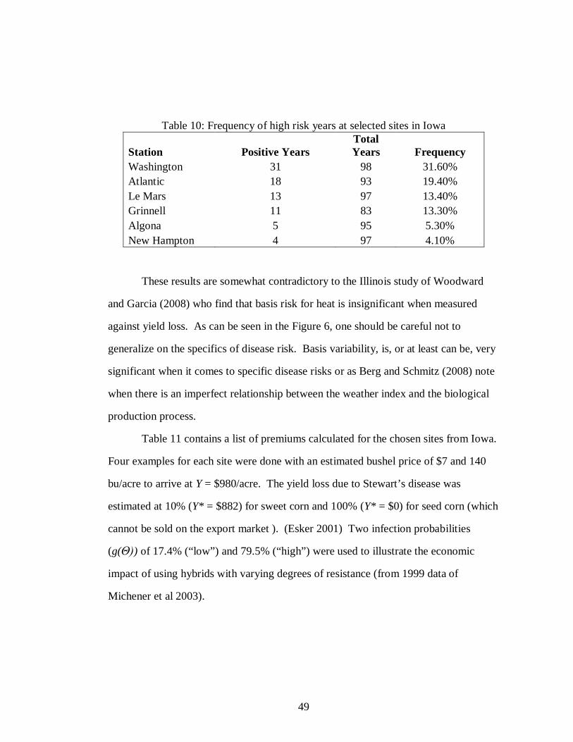
49
Table 10: Frequency of high risk years at selected sites in Iowa
Station Positive Years Total Years Frequency
Washington 31 98 31.60% Atlantic 18 93 19.40% Le Mars 13 97 13.40% Grinnell 11 83 13.30% Algona 5 95 5.30% New Hampton 4 97 4.10%
These results are somewhat contradictory to the Illinois study of Woodward
and Garcia (2008) who find that basis risk for heat is insignificant when measured
against yield loss. As can be seen in the Figure 6, one should be careful not to
generalize on the specifics of disease risk. Basis variability, is, or at least can be, very
significant when it comes to specific disease risks or as Berg and Schmitz (2008) note
when there is an imperfect relationship between the weather index and the biological
production process.
Table 11 contains a list of premiums calculated for the chosen sites from Iowa.
Four examples for each site were done with an estimated bushel price of $7 and 140
bu/acre to arrive at Y = $980/acre. The yield loss due to Stewart’s disease was
estimated at 10% (Y* = $882) for sweet corn and 100% (Y* = $0) for seed corn (which
cannot be sold on the export market ). (Esker 2001) Two infection probabilities
(g(Θ)) of 17.4% (“low”) and 79.5% (“high”) were used to illustrate the economic
impact of using hybrids with varying degrees of resistance (from 1999 data of
Michener et al 2003).

50
Table 11: Estimated premiums for different breeds of corn
Risk Sweet/Low Sweet/High Seed/Low Seed/High Washington 31.60% $5.39 $24.62 $53.88 $246.20 Atlantic 19.40% $3.31 $15.11 $33.08 $151.15 Le Mars 13.40% $2.28 $10.44 $22.85 $104.40 Grinnell 13.30% $2.27 $10.36 $22.68 $103.62 Algona 5.30% $0.90 $4.13 $9.04 $41.29 New Hampton 4.10% $0.70 $3.19 $6.99 $31.94
Conclusions
The majority of crop diseases, pest infestations, and stress originate with
specific weather events, alone or in combination. We have presented here a
prescription for insuring specific disease risks given characteristics of infection
probability, yield loss, and the historical frequency of the necessary combination of
environmental conditions needed for pathogen growth. The ideas presented in this
paper are sufficiently general, and the analytical tool (Weather Wizard) is sufficiently
flexible to enable a more thorough analysis of weather risks in combination by future
researchers. There are many hurdles to clear before we can fully harness the power of
the concepts presented in this paper, but the many advantages of weather index
insurance as a proxy for losses should reward those with the dedication to making
them a financial reality. At the very least, this paper serves to demonstrate just one
facet of the vast potential of weather index insurance as a risk management tool.
Finally, would farmers be willing to pay for insurance with such specificity as
presented here? Musshoff et al (2008) conclude, but in a somewhat different context,
that farmers do/will show a willingness to pay for weather insurance and add that the
willingness to pay goes beyond the actuarial price as presented here. Thus farmers
would not only pay the fair price for loss, but also any loading that might be added by

51
the insurer. Additionally we might also consider the role of the risk measures here in
terms of risk identification by insurers and reinsurers. These institutions do not face
single risk as do farmers but a portfolio of risk with sources pooled from many diverse
areas. (see Roth et al 2008, Turvey 2005, Miranda et al) Nonetheless, by pinpointing
the scientific relationship between weather and plant diseases or insect infestations and
identifying spatial risk profiling in terms of joint and conditional probabilities, much
of the ‘moral hazard’ problems in agricultural insurance can be alleviated.

52
Chapter 5 – Weather Index Insurance and the Geographic Variability of Risk
While a comparatively large amount of analysis has been expended on the
local effects of basis risk, or more precisely the weather/yield relationship, very little
analysis has been done about the geographic nature of basis risk, otherwise known as
the uncertainty that develops as we increase distance from a known location. To avoid
this problem, researchers sometimes base research at sites with constant elevation
(Richards, Manfredo, and Sanders 2004) and conduct projects only within a small
geographic radius (such as the World Bank project in Malawi.) Some researchers
have even suggested that farmers could hedge risk by purchasing a portfolio of
weather derivatives for established cities the CME exchange (Woodward and Garcia
2008).
Even if we had perfect understanding of how to price insurance premiums at a
given location, we would not be able to say with certainty how that risk changes
through space or how to price premiums at geographically varied locations. A more
fundamental approach is needed and this paper describes the search for a general
principle whereby risk could be accurately predicted by simple, widely available
geographic variables. By understanding the nature of how risk changes through space,
we may assess the accuracy of insurance policies written at discrete locations and
arrive at strategies for wider use of weather index insurance.
Traditional GIS methods of spatial interpolation like inverse distance
weighting are ill-fitting for several reasons. The insurance payout is a function of
temperature, but spatial interpolation methods bias the variability, and it is the
variability that as insurers we are most concerned with. Second, it is not so much the
geographic or spatial relationships that are of interest, but the geographic or spatial

53
relationships given certain weather conditions. In other words, the mean for a known
location is only of value at that location, but we need to analyze the spread of risk in a
distributed geographic area as different weather conditions prevailed on a year by year
basis. The spatial interpolation method for solving this would presumably be to
interpolate a map for each individual year of study and combine them to make a
composite. This would provide a measure of risk at each location, but this would not,
however, allow us to price payouts for unknown locations given a series of
observations in future years.
Table 12: Correlation of average of nearby stations of cumulative weather indexes
Heat Base
Station
Avg. of Surrounding
Stations Difference Correlation CDD Index (85° F): 68.41 71.51 -4.5% 0.8849 Heat Risk Event (Payout): $22.37 $27.31 -22.1% 0.7751 Rainfall Cumulative Rainfall (in.): 10.65 10.36 2.6% 0.7457 Drought Risk Event (Payout): $20.95 $22.61 -7.9% 0.6897
For illustration, some summary statistics are presented in Table 12. Listed are
the aggregate temperature and rainfall observations for Ithaca, NY for June 1st –
August 31st along with the average observation for all stations within a proscribed
radius (100 miles for temperatures and 67 miles for rainfall.) The overall averages are
similar but of course mean values are of little interest. When we examine the yearly
variation as measured by the average correlation between the base station (Ithaca) and
every other station, we find that heat is highly correlated but rainfall less so. A
familiar pattern is that when we introduce risk events (defined later), the variability
increases, not only in the averages but also in the correlation. The information

54
presented here is also for relatively common events over long date ranges; presumably
these numbers would weaken if a more specific time frame or risk event were used.
The challenge presented is to improve the accuracy of the yearly correlation.
Although it is tempting to view this data as a sterile set of statistics, insurance policies
would have profound real-world implications for farmers holding a policy. It is
crucial to accurately reimburse them in a year when they face actual losses. By taking
the payout schedule for all stations and adjusting for geographic variables, we can
potentially price insurance contracts for any given point on the map. Because of the
vast number of stations located around the country, our hopeful result is a simple
equation in which we can build upon this simple methodology and adjust for the
differences in distance, altitude, and polar coordinates to arrive at a payout for any
unknown location.
Defining the geographic area
Weather Wizard is flexible as to the distance of the radius extending from the
base station, but there are a few requirements that must be considered for a successful
trial. A number of stations are needed to provide contrast, but there are few stations
within a short distance (10 miles) of each other.
However, as we increase the radius of the circle, the area of the circle increases
exponentially. Barring any obstacles like oceans, as the radius of the circle increases,
the number of stations increases exponentially. Because we compare each station
against each other in each year, this also dramatically increases the number of
comparisons that are made, as given by the following formula:
yearsnnscomparison *2
)1(*

55
Where n is the number of stations within the selected geographic radius. The
total is subject to missing and incomplete data; many stations have only limited data,
and with longer time horizons the potential of missing data within years becomes
greater.
Table 13: Number of comparisons in Ithaca, NY for a given number of miles
Rainfall
Miles Stations
Potential
Comparisons
Actual
Comparisons
10 2 225 93 41.33%
15 4 750 223 29.73%
20 12 5850 801 13.69%
25 17 11,475 1628 14.19%
30 25 24,375 3,304 13.55%
35 35 47,250 6,921 14.65%
Heat
Miles Stations
Potential
Comparisons
Actual
Comparisons
10 2 225 23 10.22%
15 2 225 23 10.22%
20 4 750 105 14.00%
25 6 1575 220 13.97%
30 10 4125 525 12.73%
35 16 10,200 1,366 13.39%
Perhaps in acknowledgement of the periodic, unpredictable nature of rainfall,
observation stations are more densely placed and often contain more years of data. It
is very likely that temperature observations are placed more sparsely to reflect that
temperatures are considered to vary continuously over a geographic area.
The discrepancy in data for the different weather types is very pronounced, but
such factors as length of contract and number years selected will also affect the

56
percentages in Table 13. These percentages are somewhat low because of a relatively
long date range. A 92-day window is not unreasonable but offers more opportunities
for data to be missing. Also, more importantly, very few stations have data
continuously to 1926; most stations date to the late 1940s, and it’s not uncommon for
a station to have as little as one or two years of data for the entire 75 year period. If
we selected a shorter contract length (say, 15 days instead of 92) fewer stations would
be disqualified for missing data; likewise, if we only considered years after 1949, the
percentage of actual comparisons would improve markedly. This discussion is
intended to underscore the fact that even though we might define an identical
geographic area, there is often a very different spatial distribution of data within that
area depending on the parameters we select.
The advantage of this comparison-based model is that it treats all weather
stations equally and is able to include otherwise useless data. In this model the data
will be compared on a year by year basis, regardless of how many years of data are at
a particular station. The weather stations that only have a few years of data help
provide contrast for spatial distributions of risk even though it is impossible to
accurately price a contract for that station individually.
Also of pertinent interest is what these details entail for selecting a radius to
study. As the radius increases, the area of study increases exponentially (according to
the area of a circle – πr2), increasing the number of stations accordingly, which has
vast ramifications for the number of potential comparisons according to the equation
above. Since Weather Wizard is hosted on a web platform, there are limitations to the
amount of data that it can process in a single iteration - selecting a radius requires the
user to select a value large enough to offer meaningful results that will also fit within
the technical possibilities. For this paper, we are using a radius of 50 miles, which is

57
large enough to allow the inclusion of sufficient stations for both heat and
precipitation, but small enough to run properly on the Weather Wizard website.
The Regression Equation
The goal when formulating this regression equation was to try and predict the
difference in payouts in any given year between any two locations using simple
geographic variables.
(P1 – P2) = ß1 φ + ß2 (α1 – α2) + ß3 (ω1 – ω2) + ß4 (λ 1 – λ 2) + ß0 + ε
Where Px are payouts, φ is the distance between the two stations, αx is the
altitude at each station, ωx is the latitude at each station, and λx is the absolute value of
the longitude of each station (as longitudes in the western hemisphere are traditionally
negative.)
This equation is primarily a difference equation, where we are attempting to
explain the difference in payouts by the difference in altitude and geographic
coordinates. At first blush, it seems as if the φ variable, distance, is ill-suited for
inclusion. However, by imposing a condition of P1 >= P2 we may ensure symmetry
between the left and right sides of the equation; only if (P1 – P2) is strictly positive will
it reflect a potential linear relationship with φ. Furthermore, distance is a
trigonometric function of the individual latitude and longitude variables but is highly
correlated to neither. This is because it is a joint function of latitude and longitude, and
a degree of longitude is not a constant surface measurement. It is more useful to think
of the latitude/longitude coordinates as reflecting directionality, and distance as an
adjustment for increasing variability at increased distances.

58
The equation for distance is given thusly:
φ = R * Cos-1(Sin(ω1) * Sin(ω2) + Cos(ω1) * Cos(ω2) * Cos(λ 2 – λ 1))
Where R is a constant reflecting the radius of the sphere we can use to
normalize to standard units; the constant for miles is 3963.1.
What we are left with is a description of how each station compares to each
other in three-dimensional space, not only in distance (φ ) but with x and y coordinates
given by the latitude (ωx) and longitude (λ x), and z coordinate given by altitude (αx).
The initial hypothesis of these coefficients follows along the lines of common sense.
Distance (φ) should be positively correlated in both heat and precipitation, meaning
that as distance increases, so do the differences in premiums. For rainfall, the rest of
the geographic variables are indeterminate, given that coordinates and/or altitude
would seemingly have no effect on the sporadic nature of rainfall. For heat, however,
we might expect that altitude and latitude have a negative effect on risk; or, in other
words, heat risk is decreased by either an increase in elevation or more northerly
locations.
Defining the Risk Events
Choosing an event that is sufficiently general yet meaningful for all sites is
difficult, because there is no such thing as generality, as Chapter 3 tells us. A heat
event in upstate New York is incomparable to a heat event in a warmer climate. The
sheer variation of climates in America requires us to tailor our heat risk events for
each station.

59
To start, evidence indicates that temperatures above 85° F correlate with crop
yield losses. (Schlenker and Roberts 2006) Using this as a benchmark, we accumulate
a CDD index above 85° F with the mean CDD at the base station serving as the strike
value and a sliding payout for values above that. Payouts are calculated at each station
for every year data is available. Figure 7 shows the payout schedule for Ithaca, NY,
where mean CDD is 68.41.
-5
0
5
10
15
20
25
30
35
0 20 40 60 80 100
CDD
Payo
ut
Figure 7: Schedule of payouts for heat risk event
Six weather stations were selected at sites across the country according to
quality of data and the absence of major geographic obstacles within 50 miles, such as
large bodies of water or international borders. Mean CDD for those six stations vary
from 68.41 at Ithaca, NY to 720.63 in Davis, CA and are listed in Table 14.
Table 14: Mean CDD (85° F) at each location
Station
Bridgeport, NE Bethany, MO
Greenville, AL Davis, CA Ithaca, NY
Mosquero, NM
Mean CDD (85 F) 442.13 350.74 603.18 720.63 68.41 282.05

60
For precipitation, the contract is identical for all sites. We use a drought event
of less than .1” of precipitation over any 14 day period. The payoff will occur on a
sliding scale with $10 accumulating for each hundredth of an inch less that .1”, to a
maximum of $100 per event if no rainfall was recorded. Up to three non-overlapping
events are possible, and if more events occur, the variable payoffs are averaged to
normalize the payoffs to three events. Figure 8 shows the payoff schedule due to the
observed rainfall in any 14-day period, but yearly payoff amounts range from $0 to
$300 because of the possibility of multiple events.
-20
0
20
40
60
80
100
0 0.1 0.2 0.3 0.4 0.5
Precipitation per event
Payo
ut
Figure 8: Schedule of payouts for drought risk event

61
Regression Results
Table 15: Regression results for heat risk event
Station Bridgeport,
NE Bethany, MO Greenville,
AL Davis, CA Ithaca, NY Mosquero,
NM
# of Years 104 75 66 83 74 71
Mean CDD 442.13 350.74 603.18 720.63 68.41 282.05
Stations within 50
miles 19 25 21 44 35 16
N 4300 4417 3052 7255 5953 1831
R² 0.0103 0.0419 0.0010 0.0157 0.0525 0.4921
Distance -.215 (-2.22)** .118 (1.46) .094 (0.64) .285 (1.99)** .035 (1.32) .394 (1.86)*
Alt. Diff. -.011 (-2.45)** -.138 (-8.86)** -.020 (-1.03) -.020 (-6.86)** -.008 (-4.67)**
-.210
(-23.79)**
Lat. Diff. .428 (0.13)
14.897
(3.03)** -7.660 (-1.42)
31.278
(5.28)**
-15.926
(-14.41)**
60.886
(3.90)**
Long.
Diff.
-9.286
(-2.59)**
15.125
(3.52)** -2.933 (-0.49)
18.269
(4.33)** 7.852 (9.88)**
84.168
(9.84)**
Constant 52.298
(11.42)**
35.226
(9.48)**
66.999
(8.74)**
80.507
(11.99)**
20.724
(15.17)**
69.946
(8.27)**
The first thing we see when looking at these numbers is that with one
exception the R² values are abysmal, which is to say that these geographic variables
provide a very poor fit for payoff differences. Most of the difference in payoffs is
collected in the constant, even though the coefficients are quite often significant, and
unpredictably so. Localized conditions can be expected to have effects on the
latitude/longitude coefficients, as directionality within different locations might reflect
different geographic characteristics.

62
Table 16: Regression results for precipitation risk event
Station Bridgeport,
NE Bethany, MO Greenville,
AL Davis, CA Ithaca, NY Mosquero,
NM
# of
Years 104 75 66 83 74 71
Stations within 50
miles 27 33 41 70 79 35
N 7515 8693 10895 22393 34846 5770
R² 0.0104 0.0082 0.0131 0.0236 0.0074 0.028
Distance .074 (2.34)** .177 (4.94)** .0001 (0.00) .049 (8.66)** .127 (8.91)** .216 (5.12)**
Alt. Diff. -.014 (-7.23)** -.027 (-3.63)** .017 (4.13)**
-.003
(-18.51)** .009 (13.36)** .002 (0.86)
Lat. Diff. .308 (0.25) 1.821 (0.77) 2.345 (1.84)*
-1.616
(-6.58)** 3.090 (5.26)**
-16.058
(-4.73)**
Long.
Diff.
10.054
(7.99)**
10.929
(6.03)**
13.975
(11.21)**
-1.234
(-6.74)** -.741 (-1.68)* 9.48 (4.26)**
Constant 57.898
(34.48)**
54.71
(31.94)**
63.995
(41.25)**
14.614
(48.68)**
32.353
(43.74)**
66.293
(30.71)**
The two enduring relationships that can be deduced are the effect of altitude on
heat risk and the effect of distance on rainfall payoff differences. The coefficient for
altitude for the heat risk regressions is consistently negative and significant, which
makes sense – we would expect heat risk to decrease as elevation increases. The effect
of altitude on rainfall payoffs is unclear, as one might expect – rain perhaps doesn’t
consider the altitude of the land it’s falling onto. The coefficient attached to distance
for rainfall is, with one exception, significant and positive, meaning that as distance
increases the difference in the payoffs does too. Or, as distance increases, the payoffs
become less accurate. We might expect a similar result for heat, as stations further
apart produce more differentiated results, but it seems that temperatures vary

63
continuously throughout a geographic region and the directionality measures are often
of more interest.
These results may seem to be providing little beyond the very obvious – heat
risk decreases with altitude because of lower temperatures at higher elevations;
likewise, rainfall correlations decrease with distance because of the unpredictable,
periodic nature of rainfall. However, there is little evidence for other seemingly
obvious implications, like the relationship between latitude and heat risk – we would
expect that heat risk would decrease with increased latitudes, but in fact only one of
the six coefficients is negative and significant. In fact, it is somewhat remarkable how
little we can say about the relationship between simple geographic variables and
differences in downside risk. It has been assumed by many researchers that it would
be possible to provide a statistical solution to the problem of geographic basis risk;
these results belie the fact that weather may indeed defeat the ability of statistical
methods to predict.
Improving the Fit
There are a few transformations that we can do to improve the fit, which is not
purely an academic exercise if our goal is to make out-of-sample predictions for
unknown locations. The easiest way to improve the fit of the regression is to include
dummy variables for the weather stations and years.
The justification for including dummy variables is thus: it is easy to postulate
that each station is to some degree idiosyncratic; these dummy variables are intended
to catch the effects of nearby lakes or valleys, or anything else that can’t be captured
by the simple geographic variables that we use. The dummy variables for each year
isolate the amount of variability in any given year because the dependent variable is

64
strictly positive. This will account for any years in which payout differences were
more pronounced. Both of these dummy variable types may also be included in a
pricing algorithm as well, although if we are pricing a premium for an unknown
location for which there have never been weather observations, we cannot use the
variables which account for station idiosyncrasies.
In addition, the geographic variables don’t explain the difference in payouts
very well, but there is some evidence that the problem is one of scale. The difference
equation presented earlier in this paper used (P1 - P2) as the dependent variable, which
means that it is only very easy algebra to move the P2 variable to the right side of the
equation, where we can fit it with a coefficient. This improves the regression fit
markedly but necessitates difficult interpretations of the equation. First, if the
coefficient attached to the P2 variable is significantly different than one, it is difficult
to interpret what that means, because P1 and P2 are identical in nature and the matter
of which one is written first depends only on the (P1 >= P2) condition. Second, if
we’re trying to make an out of sample prediction, we can’t assume that the P1 variable
will be larger than P2, which may bias the results.
However, trying to model these effects for predictions at unknown locations
becomes problematic. Of course we cannot provide an adjustment for a station
idiosyncrasy at an unknown location. Most seriously, if attempting to make a
prediction with P1 on the right side of the equation we cannot guarantee the strict (P1
>= P2) condition. These methods may have promise, but it is still undetermined
whether or not they are statistically viable.

65
Table 17: Results of transformations in the regression equation
Out of Sample Predictions
Table 18: Out-of-sample predictions
Table 18 shows the results of out-of-sample predictions of payoffs in Ithaca,
NY for heat and rainfall including several different types of effects – first with the
simple geographic variables, then including the station and year dummy variables, and
finally when moving P2 to the right side of the equation. The predictions with
geographic variables are quite bad, but improve with the addition of the station and
year effects. The strongest effect is obtained by moving P2 to the right side of the
equations, which may make sense in some ways – the weather observations are the
strongest piece of information we have about prevailing conditions in any given year
and by taking the difference we often censor that important piece of information. In
Heat Prediction Obs. Average Difference Correlation Geo. Variables Only $25.27 $64.39 -154.8% -0.4422 With Station & Year Effects $32.20 $64.39 -100.0% 0.4623 And moving P2 to right side $67.30 $64.39 4.3% 0.8956 Rainfall Geo. Variables Only $37.34 $64.17 -71.8% 0.4294 With Station & Year Effects $51.33 $64.17 -25.0% 0.5217 And moving P2 to right side $66.81 $64.17 4.0% 0.6201
Original Incl. Station Incl. Year Incl. Station & Year P1 as Y All Effects
Rainfall DF 34841 34690 34768 34617 34840 34616R² 0.0074 0.1788 0.1056 0.2412 0.2644 0.4435Distance .127 (8.91)** .104 (7.05)** .122 (9.02)** .102 (7.13)** .133 (9.37)** .088 (6.22)**Alt. Diff. .009 (13.36)** -.027 (-4.35)** .007 (10.50)** -.0243 (-3.98)** .009 (12.87)** -.028 (-4.56)**Lat. Diff. 3.090 (5.26)** 8.155 (0.81) 3.049 (5.37)** 10.343 (1.06) 2.999 (5.12)** 17.119 (1.76)*Long. Diff. -.741 (-1.68)* 12.824 (1.73)* -.534 (-1.26) 19.805 (2.75)** -.607 (-1.38) 17.933 (2.50)**Constant 32.353 (43.74)** 23.671 (8.27)** 25.335 (2.50)** 10.075 (1.03) 30.445 (40.35)** 10.707 (1.11)P2 -- -- -- -- 1.413 (110.38)** .419 (26.27)**
HeatDF 5948 5889 5875 5816 5947 5815R² 0.0525 0.2294 0.5404 0.6134 0.6771 0.8720Distance .035 (1.32) .064 (2.21)** .008 (0.46) .086 (4.11)** .037 (1.53) .070 (3.69)**Alt. Diff. -.008 (-4.67)** -.028 (-3.35)** -.008 (-6.60)** .022 (3.59)** -.0122 (-8.14)** .035 (6.14)**Lat. Diff. -15.926 (-14.41)** -7.074 (-0.65) -11.570 (-14.69)** 35.801 (4.55)** -17.146 (-16.81)** 35.523 (4.97)**Long. Diff. 7.852 (9.88)** -24.862 (-2.52)** 5.436 (9.62)** 5.653 (0.78) 7.853 (10.71)** 12.452 (1.88)*Constant 20.724 (15.17)** 22.048 (5.34)** 8.27 (1.51) -28.215 (-4.82)** 13.025 (10.16)** -37.615 (-7.06)**P2 -- -- -- -- 1.124 (110.29)** .717 (57.20)**

66
any case, it must be said that the geographic variables seem to be useful only in the
optimization of an already robust distribution – in any successful prediction presented
herein, the “heavy lifting” is done by the station, year, and P2 effects. And in the case
of rainfall, this entire exercise has resulted in payouts that are in fact slightly worse
than the very simplistic approach taken in Table 12 of simply averaging payouts for
each station within 67 miles of Ithaca.
Of course, there are a few caveats that must be mentioned, the first being the
difficult mathematical interpretation of moving the P2 variable to the right side of the
equation. Also of note is that this prediction was only performed when Ithaca was the
station listed first (i.e. the P1 variable), the consequence of which is that the payouts
are significantly higher ($64.39 and $64.17) than the long-term averages as presented
in Table 18 ($20.76 and $20.87). Whether this has implications for the end results is
an important consideration.
Summary
There are two important implications of this paper. The first is that geographic
basis risk is a fundamental and persistent problem. Efforts to mitigate risk at diverse
locations, even using a portfolio method, will introduce too much variability and best
practice is to place a weather station in close proximity to the location of interest. This
result is somewhat surprising, in that many researchers have written papers assuming
that a solution to the problem of geographic basis risk was eventually forthcoming.
However, the search for a general principle failed, which is of interest in and of itself.
The second implication is what this entails for modeling, which is often
dependent on spatial variables for interpolating unknown values on a map. What these
results show is that traditional spatial interpolation methods that depend on spatial

67
relationships, like inverse distance weighting or kriging, may not be accurate in a local
context.
Some researchers are interested in macro-level relationships using satellite
imagery or radar data, especially in countries which have little historical data to rely
on. What these results show is that even if rainfall can be accurately quantified at one
location, the geographic distribution of risk cannot be accurately described and will be
prone to error. This is especially true for rainfall, which has the statistically
significant, positive coefficient with respect to distance. Further research into
predicting risk given known quantities must occur before spatial interpolation methods
are used.

68
Chapter 6 – Conclusions The study of weather index insurance is still in its formative stages and many
technical and theoretical hurdles are yet to be overcome. This thesis starts with
weather index insurance at its most basic level and extends the existing literature
through the examination of sophisticated pricing methods including joint risk and
geographical basis risk.
My goals in writing this thesis were to extend the methodology available for
researchers and practitioners of weather index insurance, not only by introducing a
publicly available empirical tool like Weather Wizard but also in the methodologies
presented in the “joint risk” and “geographic basis risk” chapters. Hopefully the
results and methods exhibited in this thesis will be a boon for progress in the area of
weather index insurance, which has promising applications in improving the
livelihoods of people in poor developing countries.
Prior to this thesis, it was assumed that there would be a computational answer
to the problem of geographic basis risk, but based on the results presented here that
notion has been challenged if not completely dispelled. It is a noteworthy result that
no statistical correlation could be found within small geographic areas and that best
practice is to place a weather station at each insurable site. The problem of geographic
basis risk is shown here to be a persistent and fundamental problem of weather index
insurance.
Similarly, existing literature on the topic of weather index insurance has
neglected to consider the presence of simultaneous risk events and their possible
insurability. While the methods presented in this thesis are necessarily an outline that
would need to be modified by insurers, the concepts are of undeniable value for risk
management purposes. Deciphering weather criteria for the seemingly limitless

69
number of crop pathogens, for instance, would be of immense value for both scientific
and insurance purposes.
However, because of the amount of data available via Weather Wizard, this
thesis relies heavily on computational methods that might not be available in places
that have poor records, like developing countries. The methods presented in this
document provide a theoretical background to fundamental problems (such as the
confirmation of the influence of distance on rainfall correlation), but have more value
in guidance than practical use. Although the methods presented in this paper represent
a genuine step forward for the study of weather index insurance, there is still much
work to be done.
Future Research
The development of the Weather Wizard website is likely a continuous process
and will need to adapt and grow as the theoretical basis behind weather index
insurance strengthens. It will be a challenge, to say the least, to maintain current
technology and data without a major contribution from a future graduate student.
However, Weather Wizard will likely be instrumental in processing the large amounts
of data necessary for further research into pricing weather index insurance using the
historical frequencies of the burn rate model, of which there are numerous
possibilities, especially in the area of basis risk (both local and geographic.)
In addition, another look at the problem of geographic basis risk using more
sophisticated spatial econometrics might prove fruitful. The findings of this paper
point the way forward but it is possible the relationship between simple geographic
variables and correlation might be improved using more sophisticated models than
ordinary least squares (OLS) regression.

70
Chapter 7 - Technical Specifications
Software Vendors
Weather Wizard is written in ASP.NET using Microsoft Visual Studio 2005.
The database platform used is Microsoft SQL Server 2003. On certain pages, data
may be exported to Microsoft Excel format for graphing functions and more in-depth
data manipulation. Third-party software includes NMath Core 2.2 and NMath Stats
2.1 by Centerspace Software for advanced regression statistics. Weather Wizard
incorporates Zip Code data for weather station selection supplied by Datasheer L.L.C.
through their website http://www.zip-codes.com.
On the state selection screen and again in the Basis Risk pages, the user may
also click to display geographic data in Google Earth. This feature uses KML
(Keyhole Markup Language), and requires Google Earth 4.1 to function correctly.
Data Summary
The data for this project is provided by the National Oceanic and Atmospheric
Administration (NOAA), and includes weather data from nearly 25,000 weather
stations over the years 1892 (at some stations) to 2001. Efforts are underway as of
the date of this writing (May 22, 2008) to update the database to include data up until
2006.
Many similar studies or products only use a fraction of the data available
because of concerns about the reliability of data more than 30 to 50 years old. For
Weather Wizard, a conscious decision was made to include the most data possible,
even if those data are incomplete. Metrics are in place to clean and replace data that is
missing. Appendix 1 is a summary table of the data grouped at the state level. (Data

71
is aggregated at the monthly level in this table not only because of the structure of the
database but because it may be the most reliable indicator of content.) This table
reveals for each state the amount of data available for each weather type as well as the
total number of weather stations and the average months of data for each weather
station.
Also of note in this table is that the most robust data set is precipitation data.
Daily High and Low temperatures are on average about 70% as large, and Daily Mean
temperatures 60%.

72
APPENDIX
Appendix A – Weather Wizard Screen Shots
Figure 9: Weather Wizard Main Screen

73
Figure 10: Date Selection Screen for Specific Event Risk

74
Figure 11: Temperature Insurance Worksheet

75
Figure 12: Temperature Insurance Worksheet illustrating excess heat risk

76
Figure 13: Precipitation Insurance Worksheet

77
Appendix B – Site Map for Weather Wizard
Figure 14: Flow Chart for Weather Wizard

78
Appendix C – State by State Data Summary
State Daily High Daily Mean Daily Low Rainfall Total Obs. # Stations Avg./Station
Texas 277,051 225,519 276,792 500,717
1,280,079 1671 766.06
Montana 169,727 146,977 169,584 204,062
690,350 716 964.18
California 140,584 113,741 140,464 229,878
624,667 1760 354.92
Arizona 138,690 121,209 138,519 178,467
576,885 569 1,013.86
Oregon 125,166 108,350 125,076 150,545
509,137 775 656.95
Kansas 98,506 76,660 98,508 191,682
465,356 778 598.14
New Mexico 111,857
96,661 111,779 142,713
463,010 617 750.42
Colorado 112,026 90,019 112,027 144,542
458,614 631 726.81
Washington 111,442 96,309 111,415 129,734
448,900 635 706.93
Nebraska 95,989 83,832 95,984 161,588
437,393 576 759.36
Utah 106,211 94,935 106,177 119,714
427,037 582 733.74
Missouri 96,476 88,826 96,555 143,072
424,929 512 829.94
Iowa 101,055 90,052 101,035 127,594
419,736 505 831.16
Illinois 101,055 90,052 101,035 127,594
419,736 550 763.16
Oklahoma 93,145 84,726 93,037 145,056
415,964 472 881.28
Pennsylvania 86,062
72,918 85,983 155,876
400,839 678 591.21
Wisconsin 94,756 88,907 94,715 120,419
398,797 343 1,162.67
North Carolina 88,109
76,757 88,071 131,387
384,324 480 800.68
Minnesota 90,629 78,878 90,753 118,539
378,799 388 976.29
New York 79,697 66,695 79,701 146,728
372,821 688 541.89
Idaho 93,713 82,464 93,660 95,953
365,790 482 758.90
South Dakota 87,517
77,214 87,420 112,787
364,938 370 986.32
Wyoming 90,005 71,801 89,932 104,242
355,980 513 693.92
Ohio 83,549 61,533 83,474 126,596
355,152 478 743.00
Michigan 85,134 70,452 85,077 104,863
345,526 575 600.91
North Dakota 81,607
72,005 81,567 106,126
341,305 347 983.59
Alaska 89,023 63,853 88,993 88,843
330,712 677 488.50
Arkansas 69,082 61,748 69,008 114,186
314,024 419 749.46
Georgia 71,383 58,147 71,244 111,718
312,492 376 831.10
Indiana 71,350 65,993 71,338 95,776
304,457 459 663.31

79
Florida 75,827 75,741 61,165 85,101
297,834 353 843.72
Tennessee 61,616 53,218 61,581 108,108
284,523 503 565.65
Virginia 63,179 55,368 63,080 101,592
283,219 424 667.97
Alabama 58,399 51,614 58,378 107,931
276,322 363 761.22
Mississippi 56,593 52,181 56,547 99,791
265,112 355 746.79
Louisiana 55,719 48,084 55,716 100,905
260,424 491 530.40
Kentucky 48,818 43,489 48,737 103,875
244,919 490 499.83
West Virginia 56,626
49,258 56,631 81,133
243,648 392 621.55
Nevada 62,845 49,379 62,745 64,295
239,264 365 655.52
Hawaii 32,058 14,518 31,988 153,142
231,706 675 343.27
South Carolina 48,201
42,563 48,164 66,623
205,551 219 938.59
Maryland 41,241 35,943 41,211 45,420
163,815 227 721.65
Massachusetts 30,698
24,983 30,705 53,791
140,177 208 673.93
New Jersey 31,199 26,459 31,202 46,505
135,365 176 769.12
Maine 33,113 25,762 33,108 41,109
133,092 202 658.87
New Hampshire 21,668
18,105 21,659 36,851
98,283 183 537.07
Vermont 17,610 15,340 17,597 30,647
81,194 152 534.17
Connecticut 16,526 12,802 16,525 32,717
78,570 142 553.31
Delaware 5,695 4,710 5,694 5,825
21,924 26 843.23
Rhode Island 3,435
1,759 3,439 4,178
12,811 20 640.55

80
Appendix D – Code Samples
Sample 1: Dat a Cleaning Algorithm While myReader.Read() And bSameStation itblWeatherStationCode = myReader.Item("WeatherStnCode") itblYear = myReader.Item("Year") itblMonth = myReader.Item("Month") PrcrSnowChanges = 0 If bstart And sqlstart <> itblYear Then LastYear = itblYear End If bstart = False 'SKIP if year omitted For i = 0 To yearOmit.Count - 1 If itblYear = yearOmit.Item(i) Then GoTo skip Next 'Change all 99999s to 0s on rainfall For i = 1 To DaysInMonth(itblMonth, 2006) Dim strDayCol As String = "Day" & Format(i) inin(gh, 0) = i & "/" & myReader.Item("Month") & "/" & myReader.Item("Year") inin(gh, 1) = myReader.Item(strDayCol).ToString gh += 1 If gh > (old_Year + 1) * (DayCount + 1) Then gh = (old_Year + 1) * (DayCount + 1) If myReader.Item(strDayCol).ToString = "99999" And (nature = 4) Then itblDay(i - 1) = 0 PrcrSnowChanges = PrcrSnowChanges + 1 Else itblDay(i - 1) = myReader.Item(strDayCol) End If If nature = 4 Then itblDay(i - 1) = itblDay(i - 1) / 100 End If Next 'Get starting and ending days xMonth = itblMonth xYear = itblYear xDays = DaysInMonth(xMonth, 2006) If Not switched Then If xMonth = monstart Then iStartDate = daystart Else iStartDate = 1 End If If xMonth = monend Then iEndDate = dayend Else iEndDate = xDays End If Else If xMonth = monend Then iStartDate = dayend Else iStartDate = 1 End If If xMonth = monstart Then iEndDate = daystart Else iEndDate = xDays End If End If y: For j = iStartDate To iEndDate

81
GetNumbers = 1 GetLastValue = 0 avgValue = 0.0 If itblDay(j - 1) = "99999" Then If j = iStartDate Then iStartDate = iStartDate + 1 GoTo y ' Start over with one less day... Kind of a cheater... ElseIf j = iEndDate Then itblDay(j - 1) = itblDay(j - 2) ' Last data point, again: kind of a cheater Else For ik = (j - 1) To iEndDate - 1 If itblDay(ik) <> 99999 Then GetLastValue = ik GoTo exitInnerLoop Else GetNumbers = GetNumbers + 1 End If Next exitInnerLoop: If itblDay(GetLastValue) > itblDay(j - 2) Then avgValue = (itblDay(GetLastValue) - itblDay(j - 2)) / GetNumbers ElseIf itblDay(GetLastValue) < itblDay(j - 2) Then avgValue = (itblDay(j - 2) - itblDay(GetLastValue)) / GetNumbers ElseIf itblDay(GetLastValue) = itblDay(j - 2) Then avgValue = 0 End If If itblDay(GetLastValue) > itblDay(j - 2) Then For ik = (j - 1) To (GetLastValue - 1) itblDay(ik) = itblDay(ik - 1) + avgValue Next ElseIf itblDay(GetLastValue) < itblDay(j - 2) Then For ik = (j - 1) To (GetLastValue - 1) itblDay(ik) = itblDay(ik - 1) - avgValue Next ElseIf itblDay(GetLastValue) = itblDay(j - 2) Then For ik = (j - 1) To (GetLastValue - 1) itblDay(ik) = itblDay(ik - 1) Next End If ' setting averages End If ' j not start or end date End If ' not a 999999 k = k + 1 If LastYear = xYear And DayInYear <= DayCount + 1 Then If k = 1 Then DayInYear = 1 YearCount = 0 Else DayInYear = DayInYear + 1 End If Else DayInYear = 1 YearCount = YearCount + 1 End If a_Setup(k - 1, 0) = k a_Setup(k - 1, 1) = xYear a_Setup(k - 1, 2) = xMonth a_Setup(k - 1, 3) = j a_Setup(k - 1, 4) = DayInYear a_Setup(k - 1, 5) = itblDay(j - 1) a_CrossRef(YearCount, DayInYear - 1) = itblDay(j - 1) a_Year(YearCount) = xYear LastYear = xYear Next skip: i = i + 1
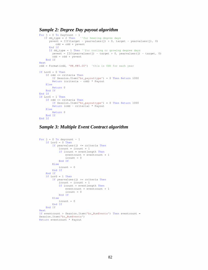
82
Sample 2: Degree Day payout algorithm For j = 0 To DayCount - 1 If dd_type = 2 Then ''for heating degree days yevent = IIf(target - yearvalues(j) > 0, target - yearvalues(j), 0) cdd = cdd + yevent End If If dd_type = 1 Then ''for cooling or growing degree days yevent = IIf(yearvalues(j) - target > 0, yearvalues(j) - target, 0) cdd = cdd + yevent End If Next cdd = Format(cdd, "##,##0.00") 'this is CDD for each year If LorG = 0 Then If cdd <= criteria Then If Session.Item("br_payouttype") = 0 Then Return 1000 Return (criteria - cdd) * Payout Else Return 0 End If End If If LorG = 1 Then If cdd >= criteria Then If Session.Item("br_payouttype") = 0 Then Return 1000 Return (cdd - criteria) * Payout Else Return 0 End If End If
Sample 3: Multiple Event Contract algorithm For j = 0 To daycount - 1 If LorG = 0 Then If yearvalues(j) <= criteria Then icount = icount + 1 If icount = eventlength Then eventcount = eventcount + 1 icount = 0 End If Else icount = 0 End If End If If LorG = 1 Then If yearvalues(j) >= criteria Then icount = icount + 1 If icount = eventlength Then eventcount = eventcount + 1 icount = 0 End If Else icount = 0 End If End If Next If eventcount > Session.Item("br_NumEvents") Then eventcount = Session.Item("br_NumEvents") Return eventcount * Payout
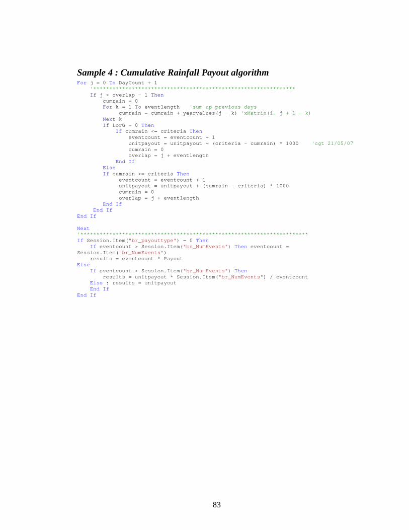
83
Sample 4 : Cumulative Rainfall Payout algorithm For j = 0 To DayCount + 1 '*************************************************************** If j > overlap - 1 Then cumrain = 0 For k = 1 To eventlength 'sum up previous days cumrain = cumrain + yearvalues(j - k) 'xMatrix(i, j + 1 - k) Next k If LorG = 0 Then If cumrain <= criteria Then eventcount = eventcount + 1 unitpayout = unitpayout + (criteria - cumrain) * 1000 'cgt 21/05/07 cumrain = 0 overlap = j + eventlength End If Else If cumrain >= criteria Then eventcount = eventcount + 1 unitpayout = unitpayout + (cumrain - criteria) * 1000 cumrain = 0 overlap = j + eventlength End If End If End If Next '*********************************************************************** If Session.Item("br_payouttype") = 0 Then If eventcount > Session.Item("br_NumEvents") Then eventcount = Session.Item("br_NumEvents") results = eventcount * Payout Else If eventcount > Session.Item("br_NumEvents") Then results = unitpayout * Session.Item("br_NumEvents") / eventcount Else : results = unitpayout End If End If

84
BIBLIOGRAPHY Agarwal, A. (2002). “A New Approach and Model for Weather Derivative Instrument based on Water
Table for Floods, Droughts and Rainfall.” Finance India 16(3): 877-914. Alaton, P, B. Djehiche and D. Stillberger. (2002). “On Modeling and Pricing Weather Derivatives.”
Applied Mathematical Finance 9(1): 1-20. Alderman, H., and T. Haque. (2006). “Insurance Against Covariate Shocks: The Role of Index-Based
Insurance in Social Protection in Low-Income Countries of Africa.” Africa Region Human Development Group, World Bank, Washington D.C.
Bardsley, P.A., A. Abey, and S. Davenport. (1984). "The Economics of Insuring Crops Against
Drought." Australian Journal of Agricultural Economics 28 (1): 1-14. Berg, E., and B. Schmitz. (2008). “Weather-Based Instruments in the Context of Whole-Farm Risk
Management.” Agricultural Finance Review 68/1:119-134. Campbell, S.D. and F.X. Diebold (2003) “Weather Forecasting for Weather Derivatives” NBER
Working Paper 10141, National Bureau of Economic Research, Cambridge, MA. Cao, M and J. Wei. (2004). “Weather Derivatives Valuation and the Market Price of Weather Risk.”
Journal of Futures Markets 24(11): 1065-1089. Changnon, S.A. and J.M. Changnon. (1990). “Use of Climatological Data in Weather Insurance.”
Journal of Climate, 3 (2): 568-576. Changnon, S.D. “Measures of Economic Impacts of Weather Extremes: Getting Better but Far from
What Is Needed—A Call for Action.” http://ams.allenpress.com/pdfserv/10.1175%2FBAMS-84-9-1231. [Accessed February 7, 2005.] Considine, G. (undated) “Introduction to Weather Derivatives” Working paper, Chicago Mercantile
Exchange, Chicago, IL. Davis, M. (2001). “Pricing Weather Derivatives by Marginal Value.” Quantitative Finance 1(3):305-
308. Dewdney, M.M., A.R. Biggs, and W.W. Turchek. (2007) “A Statistical Comparison of Blossom Blight
Forecasts of MARYBLYT and Cougarblight with receiver Operating Characteristic Curve Analysis.” Phytopathology 97:1164-1176.
Dischel, R.S. (2002). ed. Climate Risk and the Weather Market. London: Risk Books. Esker, P.D. 2001. “Geographical and Temporal Dynamics of Chaetocnema Pulicaria Populations and
Their Role in Stewart's Disease of Corn in Iowa.” Thesis/Dissertation, Iowa State University. Esker, P. D., J. Harri, P.M. Dixon, and F.W. Nutter, Jr. (2006). “Comparison of models for forecasting
of Stewart’s disease of corn in Iowa.” Plant Disease 90:1353-1357. Gautman, M., P. Hazell, and H. Alderman. (1994). “Management of Drought Risks in Rural Areas.”
Policy Research Working Paper No. 1383, World Bank, Washington D.C. Geman, H. (1999), ed. Insurance and Weather Derivatives: From Exotic Options to Exotic
85
Underlyings. London: Risk Books. Hao, J. and J.R. Skees. (July 2003). “Structuring Institutions to Share Local Weather Risks Globally.”
Selected Paper, American Agricultural Economics Association’s Annual Conference, Montreal Quebec.
Hazell, P., P. Oram and N. Chaherli. (2001). “Managing Droughts in the Low-Rainfall Areas of the
Middle East and North Africa.” EPTD Discussion Paper No. 78, International Food Policy Research Institute (IFPRI), Washington D.C.
Hazell, P. and Skees, J.R. (2006). Insuring Against Bad Weather: Recent Thinking.” In R.
Radhakrishna, S.K. Rao, S. Mahendra Dev, and K. Subbarao eds., India in a Globalizing World: Some Aspects of Macroeconomy, Agriculture, and Poverty. New Delhi: Academic Foundation.
Hess, U., K. Richter and A. Stoppa (2002). “Weather Risk Management for Agriculture and
Agribusiness in Developing Countries” In R.S. Dischel ed., Climate Risk and the Weather Market: Financial Risk Management with Weather Hedges. London: Risk Books.
Huff, F. A. and J. C. Neill. (1982). “Effects of Natural Climatic Fluctuations on the Temporal and
Spatial Variation in Crop Yields.” Journal of Applied Meteorology 21(4): 540-551. Jewson, S. and Brix, A. (2005). Weather Derivative Valuation: The Meteorogical, Statistical, Financial
and Mathematical Foundations. Cambridge, UK: Cambridge University Press. Lacoursiere, C. (2002) “Canada Opens New Pastures” Energy Risk (“Special Report: Weather Risk,”
August 2002). Leggio, K.B. and D. Lien (2002). “Hedging Gas Bills with Weather Derivatives.” Journal of
Economics and Finance 26(1): 88-100. Leiva. A. and J. Skees. (2005). “Managing Irrigation Risk with Inflow-Based Derivatives: The Case of
Rio Mayo Irrigation District in Sonora, Mexico.” Selected paper, American Agricultural Economics Association’s Annual Conference, Providence RI.
Lyon, P. (2004). “Weather Wrap-Up” Energy Risk Special Report: Weather Risk
http://db.riskwaters.com August 2004. Mafoua, E and C.G. Turvey. (July 2003). “Weather Insurance to Protect Specialty Crops Against Costs
of Irrigation in Drought Years” Selected Paper, American Agricultural Economics Association’s Annual Conference, Montreal, Quebec.
Martin, S. W., B. J. Barnett and K. H. Coble. (2001). "Developing and Pricing Precipitation Insurance." Journal of Agricultural and Resource Economics 26(1): 261-274.
Michener, P.M., N.D. Freeman, and J.K. Pataky. (2002). “Relationships between reactions of sweet
corn hybrids to Stewart’s wilt and incidence of systemic infection by Erwinia stewartii.” Plant Disease 87:223-228.
Mittler, R. (2006). “Abiotic stress, the field environment and stress combination.” Trends in Plant
Science 11/1:15-19. Muller, A. and M. Grandi. (2000). “Weather Derivatives: A Risk Management Tool for Weather
Sensitive Industries.” The Geneva Papers on Risk and Insurance 25(1): 273-287

86
Munkvold, G.P., and W.M. Carlton. (1997). “Influence of inoculation method on systemic Fusarium moniliforme infection of maize plants grown from infected seeds.” Plant Disease 81:211-216.
Munkvold, G.P., and A.E. Desjardins. (1997). “Fumonisms in Maize: Can we Reduce Their
Occurrence?” Plant Disease 81:556-565. Musshoff, O., N. Hirschauer, and M. Odening. (2008). “Portfolio Effects and the Willingness to Pay
for Weather Insurance.” Agricultural Finance Review 67/1:83-98. Nelken, Izzy (1999) “Weather Derivatives – Pricing and Hedging.” Super Computer Consulting Inc.,
Mundelein, IL. Nutter, F.W., Jr., R.R. Rubsam, S.E. Taylor, J.A. Harri, and P.D. Esker. (2002). “Use of geospatially-
referenced disease and weather data to improve site-specific forecasts for Stewart’s disease of corn in the US corn belt.” Computers and Electronics in Agriculture 37:7-14.
Odening, M., O. Musshoff, and W. Xu. (2007). “Analysis of Rainfall Derivatives Using Daily
Precipitation Models: Opportunities and Pitfalls.” Agricultural Finance Review 67/1:135-156. Odvody, G.N., N. Spencer, and J. Remmers. (1997). “A Description of Silk-Cut, a Stress-Related Loss
of Kernel Integrity in Preharvest Maize.” Plant Disease 81:439-444. Quiggin, J. (1986). "A Note on the Viability of Rainfall Insurance." Australian Journal of Agricultural
Economics, 30(1): 63-69. Patrick, G.F. (1998). “Mallee Wheat Farmers’ Demand of Crop and Rainfall Insurance.” Australian
Journal of Agricultural Economicss 32: 37-49. Richards, T.J., M. Manfredo, and D. Sanders, (2004), “Pricing Weather Derivatives,” American Journal
of Agricultural Economics 86(4): 1005-1017. Richards, T. J., J. Eaves, M. R. Manfredo. (2005). “Managing Economic Risk Caused by Insects: Bug
Options.” Agricultural Finance Review 66/1:27-46. Roth, M., C. Ulardic, and J. Trueb. (2008). “Critical Success Factors for Weather Risk Transfer
Solutions in the Agricultural Sector: A Reinsurer’s View.” Agricultural Finance Review 67/1:1-8. Ruckenbauer, P., H. Buerstmayr, and M. Lemmens. (2001). “Present strategies in resistance against
scab (Fusarium sbb.).” Euphytica 119:121-127. Runge, E. C. A., (1968). “Effects of Rainfall and Temperature Interactions During the Growing Season
on Corn Yield.” Agronomy Journal 60(5): 503-07. Rush, C.M., J.M. Stein, R.L. Bowden, R. Riemenschneider, T.N. Boratynski, and M.H. Royer. (2005).
“Status of Karnal bunt of wheat in the United States 1996 to 2004.” Plant Disease 89:212-223. Sakurai, T and T. Reardon. (1997). "Potential Demand for Drought Insurance in Burkina Faso and Its
Determinants." American Journal of Agricultural Economics, 79(4): 1193-1207. Schlenker, W., and M.J. Roberts. (2006). “Nonlinear Effects of Weather on Corn Yields.” Review of
Agricultural Economics, 28(3): 391-398. Shirley, K. (2008) “Rainfall Contract Design” Presentation at Technical Issues in Weather Index
Insurance Conference. International Research Institute of Climate and Society (IRI), New York, NY.

87
Skees, J.R., B.J. Barnett and J. Hartell. (2005). “Innovations in Government Responses to Catastrophic
Risk Sharing for Agriculture in Developing Countries.” Paper presented at the workshop Innovations in Agricultural Production Risk Management in Central America: Challenges and Opportunities to Reach the Rural Poor, Antigua, Guatemala, May 2005.
Skees, J.R., J. Hartell and J. Hao. (2006). “Weather and Index-based Insurance for Developing
Countries: Experience and Possibilities.” in Agricultural Commodity Markets and Trade: New Approaches to Analyzing Market Structure and Instability, A. Sarris and D. Hallam (eds.), Edward Elgar: Northampton, MA.
Skees, J.R., Varangis, P., Larson, D.F. and P. Siegel. (2005). Can Financial Markets be Tapped to Help
Poor People Cope with Weather Risks? in Insurance Against Poverty, S. Dercon eds., Oxford University Press: Oxford, UK.
Skees, J., S. Gober, P. Varangis, R. Lester and v. Kalavakonda. (2001). “Developing Rainfall-Based
Index Insurance in Morrocco.” Working Paper No. 2577, World Bank, Washington, D.C. Skees, J.R. (2008). “Innovations in Index Insurance for the Poor in Lower Income Countries.”
Agricultural and Resource Economics Review 37/1:1-15. Stoppa, A. and U. Hess (2003) “Design and Use of Weather Derivatives in Agricultural Policies: The
Case of Rainfall Index Insurance in Morocco.” Paper contributed at the “Agricultural Policy Reform and the WTO: Where Are We Heading?” conference in Capri, Italy, June 23-26.
Turvey, C.G. (2008). “The Pricing, Structure, and Function of Weather-Linked Bonds, Mortgages, and
Operating Credit.” Agricultural Finance Review 68/1:135-150. Turvey, C.G. and M. Norton. (2008). “An Internet-Based Tool for Weather Risk Management.”
Agricultural and Resource Economics Review 37/1:63-78. Turvey, C.G., A.J. Weersink, and C. Chiang. (2006). “The Feasibility of Ice Wine Insurance for
Ontario Ice Wine Producers.” American Journal of Agricultural Economics 88(3): 696–709 Turvey, C.G. (2005). “The Pricing of Degree-Day Weather Options.” Agricultural Finance Review
65/1:59-86. Turvey, C.G. (2002). “A Pricing Model for Degree-Day Weather Options.” Working Paper, Department
of Agricultural Economics and Business, University of Guelph, Guelph Ontario Canada. Turvey, C.G. (2001). “Weather Insurance and Specific Event Risks in Agriculture.” Review of
Agricultural Economics 23(2):333-351. USDA APHIS Factsheet. (2004). “Questions and Answers about Karnal Bunt.” Accessed on July 3rd,
2008 at http://www.aphis.usda.gov/ Vedenov, D.V. and B.J. Barnett. (2004). “Efficiency of Weather Derivatives as Primary Crop Insurance
Instruments.” Journal of Agricultural and Resource Economics 29(3): 387-403. Veeramani, V.N., L.J. Maynard and J.R. Skees. (2003). “Assessment of Risk Management Potential of
Rainfall Based Insurance Index and Rainfall Options in Andhra, India.” Selected Paper, American Agricultural Economics Association’s Annual Conference, Montreal, Quebec.
Woodward, J.D., and P. Garcia. (2008). “Basis Risk and Weather Hedging Effectiveness.”
Agricultural Finance Review 68(1):99-118.

88
Workneh, F., T.W. Allen, G.H. Nash, B. Narasimhan, R. Srinivasan, and C.M. Rush. (2008). “Rainfall
and Temperature Distinguish Between Karnal Bunt Positive and Negative Years in Wheat Fields in Texas.” Phytopathology 98:95-100.
Zeng, L. (2000). “Pricing Weather Derivatives” Journal of Risk Finance (1): 72-78.