three experimental examinations of aspects of institutions …
TRANSCRIPT

University of Rhode Island University of Rhode Island
DigitalCommons@URI DigitalCommons@URI
Open Access Dissertations
2019
THREE EXPERIMENTAL EXAMINATIONS OF ASPECTS OF THREE EXPERIMENTAL EXAMINATIONS OF ASPECTS OF
INSTITUTIONS GOVERNING NATURAL RESOURCE USE INSTITUTIONS GOVERNING NATURAL RESOURCE USE
Christopher Brozyna University of Rhode Island, [email protected]
Follow this and additional works at: https://digitalcommons.uri.edu/oa_diss
Recommended Citation Recommended Citation Brozyna, Christopher, "THREE EXPERIMENTAL EXAMINATIONS OF ASPECTS OF INSTITUTIONS GOVERNING NATURAL RESOURCE USE" (2019). Open Access Dissertations. Paper 1109. https://digitalcommons.uri.edu/oa_diss/1109
This Dissertation is brought to you for free and open access by DigitalCommons@URI. It has been accepted for inclusion in Open Access Dissertations by an authorized administrator of DigitalCommons@URI. For more information, please contact [email protected].

THREE EXPERIMENTAL EXAMINATIONS OF ASPECTS
OF INSTITUTIONS GOVERNING NATURAL RESOURCE
USE
BY
CHRISTOPHER BROZYNA
A DISSERTATION SUBMITTED IN PARTIAL FULFILLMENT OF THE
REQUIREMENTS FOR THE DEGREE OF
DOCTOR OF PHILOSOPHY
IN
ENVIRONMENTAL AND NATURAL RESOURCE ECONOMICS
UNIVERSITY OF RHODE ISLAND
2019

DOCTOR OF PHILOSOPHY DISSERTATION
OF
CHRISTOPHER BROZYNA
APPROVED:
Dissertation Committee:
Major Professor Todd Guilfoos Stephen Atlas Tom Sproul
Nasser H. Zawia
DEAN OF THE GRADUATE SCHOOL
UNIVERSITY OF RHODE ISLAND 2019

ABSTRACT
Theory alone cannot accurately describe the characteristics of successful natural
resource governance institutions. Laboratory economic experiments are needed to
analyze the characteristics and validate theories in a controlled environment. Three such
experiments on important, but frequently overlooked, aspects of institutions are reported:
time allowed for decision-making, the strength of property rights, and how resource user
groups impact each other. Chapter 1 analyzes how psychology can impact outcomes in
institutions by forcing subjects to make decisions under time pressure, something not
before analyzed in a dynamic Common Pool Resource management context. We find
users under time pressure make decisions which reduce the sustainability of shared
renewable resources. How adding parties to bargaining affects outcomes is addressed in
Chapter 2, which finds efficiency is not reduced when there are no property rights. In
fact, adding a third party to a bargain promotes more efficient outcomes in negotiations
between two parties something traditional theory does not predict. The impact is robust to
the completeness of the information participants have available. Chapter 3 is motivated
by a lack of research on how Common Pool Resource management regimes perform
when different groups of users interact. My experiment discovers the impacts
neighboring user groups have on each other. While self-managing shared resources can
lead to better outcomes, neighboring groups have a negative impact on each other. Such
externalities had not been determined by previous field research on CPRs nor had they
been deduced theoretically. Experimental examinations of three aspects of resource
governing institutions report results theory alone cannot.

iii
ACKNOWLEDGMENTS
I sincerely thank my advisor Todd Guilfoos for all the assistance, guidance, and
reviews he provided throughout the completion of this dissertation. The writing, analysis,
and experimental design within this work would be far lesser were it not for his helpful
guidance, comments, and making time to meet with me. Additionally, alerting me to
funding opportunities made my education possible.
I thank my core dissertation committee members Stephen Atlas and Thomas Sproul
for the guidance they provided me during this process. I also wish to thank Hiro Uchida,
Austin Humphries, and Elizabeth Mendenhall for their help during the project.
César Viteri Mejía and Conservation International made Chapter 3 possible and I
hope it goes a little way to thanking them for all they allowed me to do.
Finally, I wish to thank Beth Herrmann and my parents Irene and Michael Brozyna
for always supporting me and giving me the opportunities to achieve anything.

iv
PREFACE
Manuscript Format is in use in the following chapters. Chapter 1 was submitted on
30 September 2017, accepted 15 March 2018, and published by Nature Sustainability 18
April 2018. Chapter 2 is intended for submission to the American Economic Journal:
Microeconomics. Chapter 3 is intended for submission to the Journal of Environmental
Economics and Management. All three chapters describe the findings of laboratory
economic experiments.
Chapter 1 investigates the impact of time pressure on the management of a common
pool resource. Survival analysis results indicate sustainable management becomes less
likely when users are forced to make decisions under time pressure.
Chapter 2 examines the impact property rights have on bargaining outcomes. In a
context of no legal property rights, I vary the number of people able to take a good from
its owner and the information players have about the value of the good to each other. I
find the addition of a second taker improves our measure for economic outcomes and
incomplete information does not have a significant impact.
Chapter 3 determines the impacts of self-managing fishery management
organizations. Self-managing groups perform better than suboptimally exogenously
managed groups. Management groups interacting with each other negatively impact each
other’s welfare.

v
TABLE OF CONTENTS
ABSTRACT .................................................................................................................. ii
ACKNOWLEDGMENTS .......................................................................................... iii
PREFACE .................................................................................................................... iv
TABLE OF CONTENTS ............................................................................................. v
LIST OF TABLES ...................................................................................................... vi
LIST OF FIGURES ................................................................................................... vii
CHAPTER 1 .................................................................................................................. 1
SLOW AND DELIBERATE COOPERATION IN THE COMMONS ................ 1
CHAPTER 2 ................................................................................................................ 26
EFFICIENCY WITHOUT PROPERTY RIGHTS: DO MORE THIEVES LEAD
TO MORE THEFT? ............................................................................................ 26
CHAPTER 3 ................................................................................................................ 61
UNITED WE RISE, DIVIDE WE FALL: EMPOWERING RESOURCE USERS
AND LOCALIZING MANAGEMENT .............................................................. 61
APPENDICES ........................................................................................................... 125

vi
LIST OF TABLES
TABLE PAGE
Table 1.1. Survival Analysis. .......................................................................................23
Table 1.2. Extraction Analysis ....................................................................................24
Table 2.1. Ownership Analysis. ..................................................................................51
Table 2.2. Bribes Proposed in Negotiations. ...............................................................53
Table 2.3. Proposal Analysis. .....................................................................................54
Table 2.4. Bribes Proposed in Complete Information Negotiations. ..........................56
Table 3.I. Predicted individual harvests at the Nash Equilibrium and socially optimum.
....................................................................................................................................107
Table 3.II. The costs of enforcement effectiveness. .................................................108
Table 3.III. The average values of variables from the experiment. ..........................109
Table 3.IV. Incomes. .................................................................................................110
Table 3.V. Harvesting. ..............................................................................................112
Table 3.VI. Management Regime. ............................................................................115
Table 3.VII. Regulation Violations. ..........................................................................117
vii
LIST OF FIGURES
FIGURE PAGE
Figure 1.1. The average size of the group account at the beginning of each period. ...25
Figure 2.1. Diagrams of a round of the 3-person treatment of the experiment and the 2-
person treatment. ..........................................................................................................57
Figure 2.2. The proportion of original owners of the token maintaining possession of the
token, by group size. ...................................................................................................58
Figure 2.3. The proportion of original token owners maintaining possession until the end
of the first bargaining negotiation, by information. ....................................................59
Figure 2.4. The proportion of original owners maintaining possession of the token until
the end of the first bargaining negotiation. .................................................................60
Figure 3.1. The relationship between group treatment and profit levels. .................120
Figure 3.2. The relationship between management and profit levels. ......................121
Figure 3.3. The relationship between group treatments and overall harvest levels. .122
Figure 3.4. The relationship between management and overall harvest levels. .......123
Figure 3.5. The relationship between the group treatment and proportion of group
members who exceed the harvest cap. ......................................................................124

1
CHAPTER 1
Published in Nature Sustainability, April 2018
Slow and Deliberate Cooperation in the Commons
by
Chris Brozynaa, Todd Guilfoosa, Stephen Atlasb
aEnvironmental and Natural Resource Economics; bMarketing
University of Rhode Island
1 Greenhouse Road, Kingston, RI 02881, USA

2
Abstract We test how fast and slow thought processes affect cooperation for sustainability by
manipulating time pressure in a dynamic common pool resource experiment. Sustainable
management of shared resources critically depends on decisions in the current period to
leave enough stock so that future generations are able to draw upon the remaining limited
natural resources. An intertemporal common pool resource game represents a typical
dynamic for social dilemmas involving natural resources. Using one such game, we
analyse decisions throughout time. We find that people in this context deplete the
common resource to a greater extent under time pressure, which leads to greater
likelihood of stock collapse. Preventing resource collapse while managing natural
resources requires actively creating decision environments that facilitate the cognitive
capacity needed to support sustainable cooperation.
Overextraction of natural resources in the present can lead to negative consequences for
society and is at odds with most definitions of sustainable development (1). According to
Pearson (2), "the core of the idea of sustainability is the concept that current decisions
should not damage prospects for maintaining or improving living standards in the future.”
Essential for sustainability and important to many aspects of human and animal behavior
(3-6) is cooperation. Societies with imperfect, incomplete, and shared property rights face
social dilemmas characterized by conflict between individual and collective interests.
Cooperative solutions in social dilemmas require individuals to overcome selfish myopic
incentives to achieve better social outcomes. Across many social dilemmas, myopic
resource use often yields immediate, tangible, and easy to understand benefits; while
long-term cooperative and sustainable stewardship of the resource involves more thought,
planning, and coordination, along with benefits that are less certain and harder to
calculate (7). Understanding how cognitive pressures influence common pool resource
(CPR) outcomes is vital for designing interventions to prevent resource collapse and
support sustainable collective decision processes.

3
Effective stewardship of the commons requires understanding how institutions
and cognitive factors contribute to cooperation. An expansive literature considers which
institutions can establish cooperation in CPRs and why these institutions work (8-12).
While institutions have been rigorously explored in relation to CPRs, less is known about
what cognitive factors and decision environments produce sustainable cooperation in
CPRs. One particularly salient question is: do fast (intuitive) or slow (deliberative)
thought processes better support sustainable use of a common pool resource? We find
experimental evidence that groups drawing on a common pool resource are less likely to
cooperate under time pressure. Instead, a slower, more deliberative, decision process
supports cooperation which extends the life of the common pool resource and improves
social welfare.
Our experiment uses time pressure manipulation on an intertemporal CPR. While
much of the previous experimental work on social dilemmas and cognition has focused
on one-shot games, natural resources are often characterized as stock variables (ex.
wetlands, fisheries, groundwater) which are not independent of human behavior in
previous periods. These natural assets also cannot be easily regenerated if collapse
occurs. By tracking a stock of resources in our experiment we can evaluate when group
behavior causes collapse of the resource which is paramount in understanding sustainable
development, the reconciliation of society’s goals and limits of the earth’s natural
resources (13,14). We have found only one other intertemporal experiment using time
pressure which examines intertemporal preferences (15) and no previous experiments
involving intertemporal social dilemmas and cognitive manipulations, such as time
pressure. The dynamic CPR game we employ allows us to determine how cognitive
scarcity, that is present in each decision time frame, impacts the depletion and survival of
shared stocks over time. Our experiment further tests whether fast and slow thought
processes behave similarly in dynamic CPRs to one-shot social dilemmas.
Common pool resource decisions – and resource decisions in general – are
frequently made by individuals who face cognitive constraints. For example, the
condition of poverty inhibits farmers’ ability to make good decisions due to cognitive
resources being consumed by financial concerns, an equivalent of losing 13 IQ points
(16). Risks from the natural system, such as weather variability and droughts, also tax

4
mental resources (17). Recent research suggests that scarcities of time and money focus
our cognitive system on these particular scarcities, leaving little cognitive bandwidth left
to solve other problems (18-20). This may make an escape from poverty more difficult,
as the condition of poverty causes poor communities to heavily discount future
consequences of extraction behavior: cognitive scarcities contribute to poverty traps (21).
One efficient strategy when faced with cognitive constraints is to apply heuristics, fast
and simple rules, which simplify the decision environment. These strategies adopted by
subjects in dynamic CPRs under limited cognitive resources could have important
implications to the sustainability of natural resources.
It is common for experimenters to use time pressure to shine a light on the innate
thought processes of individuals. As a cognitive constraint, time pressure is used to
distinguish between fast instinctive strategies and slow deliberative strategies in the dual
process theory of cognition (22-26). Through applying time pressure to participants’
decisions we can determine if fast, instinctive strategies are more sustainable than slow,
deliberative ones.
There are two types of cooperation in a game theoretic setting: pure cooperation,
which is cooperation when defection strictly maximizes payoffs (ex. one-shot social
dilemma games), and strategic cooperation, which is cooperation that can be long-run
payoff maximizing depending on the choices of others (ex. coordination games).
Previous studies find evidence of increased cooperation under time pressure in one-shot
social dilemmas (27-30). Viewed through a dual process theory of cognition this
cooperation is observed when people sometimes adopt a cooperative heuristic in social
dilemmas. This dual process theory of cooperation is stated in the Social Heuristics
Hypothesis (SHH) (5,6,31). SHH predicts that deliberation can undermine pure
cooperation but may support strategic cooperation if the context is sensitive for intuitive
thought processes (31). Under certain distributional assumptions of deliberation costs,
intuitive defectors may use deliberation to switch to cooperation when future
repercussions exist (32). A recent meta-study (30) finds evidence for the prediction of
increased cooperation in social dilemmas when people rely more on intuitive thought
processes and also finds no effects on cooperation of cognitive manipulation (ex. time
pressure or cognitive load) in games with the potential of future benefits. Though, there is

5
a recent study finding decreased cooperation with time pressure which is attributed to
confusion (33). According to SHH, deliberation would either have no effect or increase
cooperation in our setting because cooperation can be payoff maximizing over the life of
the common pool resource, similar to a coordination game. Our experiment adds a new
perspective to the observed behavior of individuals subjected to cognitive scarcities in a
dynamic social dilemma.
Utilizing a between-subject comparison test (between participants under time
pressure and participants without a time constraint) we find participants behave more
myopically when limited by time constraints, which is consistent with SHH. Thus,
common pool resources have a higher probability of failure when managed by people
under cognitive scarcities, a finding which contrasts the findings from previous time
pressure experiments. We explore three potential reasons for this result which include:
errors in judgment (34,35), slow adjustment of extraction strategies during the game (36),
and intuitive heuristics for myopic extraction (5,6,31). Our results highlight the benefits
of examining intertemporal dynamics over one-shot games to understand how cognition
and cooperation unfolds to promote sustainable development.
Dynamic CPR Model
There are numerous economic experiments with dynamic CPRs that investigate different
institutions which propagate cooperation (37,38). Our experiment uses a dynamic CPR
model used by Kimbrough and Vostroknutov (39). This model considers an inexhaustible
private resource and an exhaustible shared resource. Socially optimal resource
exploitation in this game requires drawing heavily from the shared resource early and
preserving it as time passes. In each period, n players simultaneously remove tokens from
an inexhaustible private account and a shared exhaustible group account with the
constraint that only 60 tokens in total can be taken in a period. Tokens from the group
account are worth twice as much as tokens from the individual account. Each group
member i chooses the number of tokens to extract, ���, from the group account at time t.
The sum of the group members extraction is �� = ∑ ������ . The group account acts as the
stock of a common pool resource in the experiment and the private account acts as the
opportunity cost of extraction.

6
The group account replenishes at a rate, β, each period, multiplied by the
difference between the remaining group account balance and a maximum size of the
group account, � . Thus the group account, �, evolves over time according to the
following formula: � = �� − ��� + �(� − �� − ���). The size of the group
account in the present period directly depends on the size of the group account in the past
round and the decisions made by group members in that round. To realize regrowth of the
group account, groups must maintain a group account level above a threshold, �.
Whenever the group account is reduced below this threshold there ceases to be any
regrowth in the group account and the resource collapses. In our experiment β was set at
0.25, the minimum threshold, �, was set equal to 30 tokens, and � was set to 360 tokens.
We parameterize a relatively small regrowth rate in our experiment so that the
symmetrical Subgame Perfect Nash Equilibrium (SPNE) is to exhaust the resource as fast
as possible though gains for the group can be higher if they do not exhaust the resource.
The socially optimal strategy in this game is to maintain the group account indefinitely to
prevent the collapse of the group account. The path of the socially optimal extraction
depends on the parameters of the experiment and consists of a set of group account
dependent choice rules, detailed in the Methods section.
This model describes situations where societies discover a virgin resource, extract
much of it, and then attempt to jointly conserve the remaining resource. The presence of a
threshold, below which the stock will not regenerate, is also a pillar of ecological theory
(40) and is descriptive of many real-world common pool resource dilemmas.
Results Figure 1.1 shows the evolution of the average group account (stock) size for time
pressure and non-time pressure groups. The lower stock path of time pressure groups
indicates greater extraction and lower survival rates of group accounts in the time
pressure treatments as compared to those under no time pressure. This suggests that time
pressure leads to less cooperation and shorter survival of the common resource.
We use a Cox proportional hazard model to estimate the treatment effect of time
pressure on the probability of failure of the group account. This method of survival
analysis is commonly employed in medical research to measure causal effects on the

7
probability of an event, such as death or relapse, and in economics and political science
to evaluate duration data (41-44). The model is appropriate to analyze the event of failure
of the group account in our experiment since the timing of collapse is a type of duration
data.
Analysis at the individual level in Table 1.1 suggests an effect from the
imposition of time pressure (group level analysis is provided in Supplementary Table 1).
We find that individuals exposed to time pressure face an increased rate of failure of
101.3% (2.013 = ��.���, � < 0.01) over the control group in Table 1.1, column 2. This
is sometimes referred to as the hazard ratio in survival analysis studies. A similar pattern
is present for individual differences in Cognitive Reflection Test (CRT). An increase in
correctly answered CRT questions reduced the rate of group account failure by 79%
(p<0.05). The coefficient on the percentage of CRT questions answered correctly
indicates that participants who do not repress their intuitive thought process induce a
greater probability of failure of the group account. This finding is also consistent with
the average treatment effects of time pressure. The rate of increase in hazard ratio is
roughly equivalent across time periods with the difference in hazard ratios being
proportional, which is an important assumption in the Cox proportional hazards model.
The results suggest that time pressure significantly increases the failure rate of the group
account in the intertemporal CPR game which adds a different finding from much of the
existing literature on cooperation and intuitive decisions in one-shot social dilemmas.
Extraction Behavior
We also explain the effect of time pressure on the deviation of observed extraction from
the optimal extraction behavior (��� !""# %�& '!" �(&)!�& �* −%+,�)-�. �(&)!�& �*). We analyze this difference in extraction behavior because the
socially optimal extraction path is group account dependent and incorporates the level of
the group account as a decision making variable that is nonlinearly related to extraction
decisions. Using a simpler extraction measure, like the number of group tokens
extracted, may be misleading as participants adjust to changing group account levels
across rounds of the game. In the following analysis we only include rounds of the game

8
before exhaustion of the group account since the observed behavior after exhaustion is
trivial.
In Table 1.2 we find that time pressure induces greater extraction than the control
group. A negative coefficient indicates the variable increases extraction relative to the
social optimal, which in turn would increase the relative risk of collapse of the resource.
The treatment effect is statistically weak without any controls, which suggests the time
within game is important to the size of the treatment effect. As a robustness check, the SI
reports results including subjects and groups who violated the time limit to test whether
results are explained by systematic differences between the participants who meet the
time constraint versus those who do not (Supplementary Table 3). In some one-shot
games there is a loss of support for intuitive cooperation when including these
participants. We find attenuated estimates of our treatment effect, though they are still
statistically significant with the inclusion of all participants. We also take a further look
at round differences in Supplementary Table 4. The coefficient on time pressure is
negative though the coefficient on CRT score is not statistically significant. Combined
with our survival analyses (Table 1.1, and Supplementary Tables 2, 3, and 4) this gives us
some confidence that the cognitive scarcities in the dynamic common pool resource game
induce less cooperative behavior and increase the risk of group account failure through
greater myopic extraction.
Discussion
Our results indicate one domain in which intuitive judgment under limited
cognitive resources leads to more myopic behavior, to the detriment of the individual and
group welfare. We find in an intertemporal social dilemma game, participants with
cognitive scarcities have a propensity to extract more from a shared resource stock. This
result provides empirical evidence of when individuals are deliberatively cooperative,
which has previously drawn almost exclusively on static social dilemma experiments
(5,27,28). In an intertemporal setting, individuals require the cognitive bandwidth for
sustainable management of the resource, and deliberation supports cooperation in this
setting.

9
Since many common pool resource situations are intertemporal in nature, our
results are more germane to these contexts than those of traditional one-shot games
(27,28). Such one-shot games are limited in their ability to capture the development of
intertemporal dynamics, which can have large impacts on sustainable development. In
one-shot games the logical action is to extract as much as possible. However, in
intertemporal games with repeated interactions cooperating in maintaining the resource
becomes a more viable strategy (45); a phenomenon which helps explain the success of
some common pool resource management programs (46). So it is interesting that the
imposition of time pressure decreases the probability of survival of group accounts in our
experiment, which suggests these CPR success stories were in spite of intuitively myopic
behavior.
We explore three potential reasons for the contrast between our results and those
of prior static non-cooperative games. The first possibility is that people make more
mistakes when confronted with a difficult problem under time pressure (34, 35). Such
stochastic mistakes may increase the variance in play from participants and the group
account may be inadvertently exhausted. To evaluate the variation in extraction behavior
we compare the absolute value of the deviation of extraction decisions between rounds
(/+,�"0&� 1�- !& �* = | ��,� − ��,��| ) in Supplementary Figure 1. A greater value of
the absolute deviation from the time pressure treatment would indicate that stochastic
behavior, or random mistakes, may play some role in additional failure of groups in the
survival analysis. Our results suggest that stochasticity in choice is similar between time
pressure treatments. This however does not suggest that other mean shifting errors in
extraction do not exist.
A second explanation for the departure from past one-shot game results is that the
design of the game encourages large extraction decisions at the beginning of the game
and cooperation requires restraining extraction behavior once the group account nears the
threshold for failure. The initial extraction behavior could induce inertia in participants
under time pressure leading to a slower adaptation to optimal levels of extraction. Alós-
Ferrer et al. (36) found that inertia as an automatic process conflicts with a more rational
deliberative one, consistent with the dual process view of decision making. We can use
the change in extraction behavior to analyze inertia as well as variance in individual

10
extraction behavior. A smaller absolute value of the difference in extraction decisions
indicates greater inertia in extraction decisions. We find no difference in inertia between
time pressure treatments, which puts serious doubts on inertia as an explanation for
increased extraction and greater failure of CPRs (Supplementary Figure 1).
A third explanation, the main hypothesis for interpretation of these results, is that
the dynamic aspect of the game affects intuitive cooperation among subjects. The data
from our experiment supports the proposition of quick and fast myopic behavior in the
commons. Our finding is consistent with the SHH (5,6), wherein deliberation can
sometimes increase cooperation in settings where cooperating can be a long run payoff-
maximizing strategy. Such an increase in cooperation can be favored by natural selection
or learning – and thus is expected to occur – if cooperation is typically long-run
advantageous and intuition is sufficiently sensitive to context (31), or if most interactions
are one-shot and the distribution of deliberation costs satisfies certain conditions
(32). Deliberation promotes cooperation when it leads people to attend to the features of
the dynamic CPR which realize cooperation as a more efficient strategy. If people only
really confront the nature of the collapsing resource when they have time, deliberation
would override myopic impulses.
Many decisions in our society can be characterized as dynamic choices under
cognitive scarcities. Our research provides insights into instinctive human behavior,
enabling us to shed light on whether humans behave more myopically under temporally
dynamic common pool resource scenarios with quick and fast decision processes. This
may well mean that cooperation in the commons is more difficult to sustain because of
intuitively myopic behavior and the use of policy tools becomes even more important to
combat over-extraction in the commons. It is also unclear how to provide the cognitive
bandwidth necessary to support cooperative behavior since it can be presented through a
combination of factors, though efforts to mitigate these stressors for individuals operating
in a common pool resource context could provide an important support tool to sustainable
collective management.
The results also highlight the implications of generalizing results of one-shot
games to situations that involve intertemporal trade-offs, or repeat interactions, when
considering sustainability. One-shot games are poor substitutes for dynamic games when

11
exploring cognitive processes of human behavior and sustainability. To evaluate the
importance of deliberation in thought processes to cooperation in common pool resources
more aspects of these games need to be explored. Specifically, there is a need to
investigate how group size, uncertainty in natural systems, and institutions affect the
cognitive thought processes and cooperation to support sustainable management.
Methods
Data
A total of 120 undergraduate students were recruited at a public university in the
northeastern United States and paid based on their performance in the game. Participants
played three cycles of the intertemporal CPR game in the Spring and Fall of 2016, a cycle
is one set of rounds of the same CPR game with the same group. In each cycle, a
participant extracted tokens from a group account shared with 3 other anonymous
participants (a representative decision screen is shown in Supplementary Figure 4). The
last round (decision period) in each game was randomly predetermined and not
communicated to the participants to avoid last round effects. Participants were randomly
and anonymously regrouped after each cycle into a new group.
Participants received a show-up fee of $10 and the average payout at the end of
the game was $18.70. The payout was based on each individual token taken from the
private account yielding a return of 0.8 cents while the tokens taken from the public
account yielded 1.6 cents each. The economic experiment software Z-tree (47) was used
to run the experiment. There were three cycles in the experiment with a predetermined
fixed length; the first cycle lasted 12 rounds, the second cycle lasted 15 rounds, and the
third cycle lasted 8 rounds. Participants were not told how many rounds to expect or that
there would be multiple cycles during the experiment.
Prior to the game, participants answered a three question Cognitive Reflection
Test (CRT) (shown in Supplementary Figure 3) under a 90 second time constraint (48).
The Cognitive Reflection Test can determine whether participants can suppress an
intuitive answer which uses little conscious deliberation (“System 1” spontaneous,

12
intuitive thinking) and employ a slower and more reflective cognitive process (“System
2” processes requiring mental effort and reasoning) when making decisions. If a subject
did not answer all three of the CRT questions before the end of the 90 seconds then they
were recorded as having not finished the CRT and as having answered none of the
questions correct.
In addition to the CRT, participants answered demographic questions (as shown
in Supplementary Figure 2). Next participants were given instructions about the dynamic
CPR game (a representative copy of these instructions is provided in the Supplementary
Information). The experimenter read the instructions to the participants, who were
required to correctly answer 3 comprehension questions to confirm their understanding of
the game. Experience with other economic experiments, time to complete the
comprehension questions, CRT scores, gender ratios, and areas of study of the subjects
were similar between treatment and control groups. Indicators for whether a participant
was majoring in environmental economics or biology were included because of the
potential for effects from their educational program of choice on their decisions.
The participants in half of the experimental sessions were exposed to time
pressure constraints with a 7-second per round decision time limit. This constraint was
chosen because the decision times of subjects within sessions without time pressure
indicated that it would be a binding constraint for the majority of them. There was a clock
visible to subjects counting down the time and the decision screen disappeared after the
7-second limit was reached. Time pressure was instituted by requiring participants to
make extraction decisions within 7-seconds, and if the time constraint was violated then
the participants earned zero tokens (public or private) for that round. When subjects
violate the 7-second time limit no tokens are taken from the group account for that
subject. To ensure differences in extraction decisions are active choices rather than
inaction, 31 out of 2,440 observations where subjects do not make a decision within the
time constraint are excluded in the analysis. Similarly, 16 out of 90 groups with a subject
who did not enter an extraction decision within the time constraint are excluded from the
survival analysis so that any interdependency between that zero-extraction observation
and overall survival is not biased. Most participants in sessions without a time constraint
took longer to make a decision than the time constraint would have permitted (indicating
13
the 7-second time constraint was binding on average); we find the difference in mean
decision time between treatment and control groups is statistically significant at the 1%
level using a Mann-Whitney two sample statistic test.
We employ a series of statistical tests to estimate the treatment effect of time
pressure and the effect of greater CRT scores on cooperative behavior to understand the
cognitive underpinnings of cooperation in a dynamic CPR.
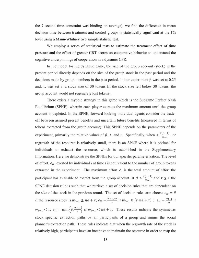
In the model for the dynamic game, the size of the group account (stock) in the
present period directly depends on the size of the group stock in the past period and the
decisions made by group members in the past period. In our experiment β was set at 0.25
and, �, was set at a stock size of 30 tokens (if the stock size fell below 30 tokens, the
group account would not regenerate lost tokens).
There exists a myopic strategy in this game which is the Subgame Perfect Nash
Equilibrium (SPNE), wherein each player extracts the maximum amount until the group
account is depleted. In the SPNE, forward-looking individual agents consider the trade-
off between assured present benefits and uncertain future benefits (measured in terms of
tokens extracted from the group account). This SPNE depends on the parameters of the
experiment, primarily the relative values of �, �, and n. Specifically, when < 3(��)4� �3 , or
regrowth of the resource is relatively small, there is an SPNE where it is optimal for
individuals to exhaust the resource, which is established in the Supplementary
Information. Here we demonstrate the SPNEs for our specific parameterization. The level
of effort, ���, exerted by individual i at time t is equivalent to the number of group tokens
extracted in the experiment. The maximum effort, �, is the total amount of effort the
participant has available to extract from the group account. If � > 3(��)4� �3 and � ≤ � the
SPNE decision rule is such that we retrieve a set of decision rules that are dependent on
the size of the stock in the previous round. The set of decision rules are: choose ��� = �
if the resource stock is �� ≥ *� + �; ��� = 49:;�3� if �� ∈ =�, *� + �) ; ��� = 49:;
� if
�� < �; ��� = min A�, 49:;� B if �� < *� + �. These results indicate the symmetric
stock specific extraction paths by all participants of a group and mimic the social
planner’s extraction path. These rules indicate that when the regrowth rate of the stock is
relatively high, participants have an incentive to maintain the resource in order to reap the

14
benefits of future periods of the stock and the growth of that stock. When the regrowth
rate is relatively small and � < 3(��)4� �3 and � ≤ � then the optimal decision rule is to
extract ��� = min {�, 4�}. This extraction path drives the stock to extinction and is similar
to the Nash Equilibrium in the prisoner’s dilemma game. The proof of the optimal
decision rule for our experiment can be found in the Supplementary Notes of our SI. In
our parameterization, with a low regrowth rate of the stock, the SPNE decision rule is to
extract ��� = min {�, 4�}. Though multiple equilibria can exist, invoking the Folk Theorem
(41), if subjects are sufficiently patient the SPNE can coincide with the social optimal
path of extraction. Through the lens of SHH, the Folk Theorem could operationalize
strategic cooperation because individuals can maximize their own payoffs through
cooperation. This is true if individuals are patient and expect future gains in later time
periods provided others cooperate, as current period cooperative decisions are more likely
to sustain later cooperation. For certain values of the parameters �, �, and n the selfish
SPNE could also coincide with the socially optimal strategy. For instance, when regrowth
of the group account is relatively high the private benefits from cooperating with group
members can outweigh the private benefits from extracting the resource to collapse,
therefore creating a game where social cooperation and the SPNE are equivalent.
In our experiment, the group account starts with 360 tokens in it and each group
token extracted is subtracted from the total amount of tokens in the account. After each
round of decision making, the resource stock grows according to the formula (360 - X)/4
tokens, where X is the stock of group tokens. Therefore, at the beginning of the next
period, there will be X + (360 - X)/4 tokens in the group account. If the total number of
tokens in the group account ever falls to fewer than 30 tokens, the threshold �, the group
account will cease to replenish.
Econometric Methodology
Survival analysis is the appropriate tool to analyze the time to exhaustion of the group
account. Ordinary linear regression would require that the group exhaustion times be
transformed to account for their strictly positive values and for the censoring of the data.

15
Therefore, survival analysis is more appropriate in our context rather than ordinary linear
regression (44).
The semi-parametric Cox proportional hazards regression describes the
dependence of failure risk at any time, t, on the covariates in the regression (41). The Cox
model is popular, flexible, and does not assume specific probability distributions until
events occur, leading to the advantage of not needing to parameterize time dependency
(43). The Cox proportional hazards model is the most commonly used modeling
procedure for survival/censored data and covariates.
In the Cox proportional hazards model, E(&) is the survivor function, E(&) =F) (& ≤ G) and H(&) is the hazard at time t, where H(&) = lim∆�→�
LM (�NOP�Q∆|OR�)∆ = S(T�).
We can use a set of k covariates in X and recover the coefficients of vector � which tell
us about the hazard of failure for a specific covariate. The hazard rate is H(&|T) =H�(&)�UV, where � is a px1 vector of unknown coefficients and H�(&) is an unknown
function for the baseline cumulative hazard function when X=0. The hazard ratio is
thus H(&)/H�(&) and "* X Y(�)YZ(�)[ = �T. This holds for all individuals so that
"* Y\(�)Y](�)= �(T − T�) for individuals i and j.
In the Cox model, baseline hazard rates vary over time, but the hazards for
different covariate values are assumed to be proportional or constant over time. The
proportions are also assumed to hold for all periods of t and between all individuals (42).
The Cox proportional hazards model implies that an independent variable shifts the
hazard by a factor of proportionality. This time invariant proportionality assumption
implies that the size of that effect remains the same irrespective of when it occurs. If this
assumption is violated, the outcomes can be significantly biased coefficient estimates
(and reduced power from significance tests, leading to inefficient estimates) and therefore
overestimated or underestimated variable impacts (42). We test for proportionality using
Schoenfeld and Deviance residuals and find that for our data the proportionality
assumption holds.
We use the Breslow approximation to handle ties in event times. It is the simplest
approximation to the probability that an individual had an event, given that an event
occurred at that time. While it is the simplest, it also the most conservatively biased (it

16
estimates coefficients too close to zero) and was chosen for such (44). In addition, we
cluster standard errors in our analysis by the unit of observation. Observations at the
individual subject level can have errors which are correlated and therefore clustering is a
common technique for statistical inference of the significance of the recovered
coefficients.
In Table 1.2 we present ordinary linear regressions of the deviation of extraction
decisions to the social optimal extraction decision, including a series of controls. The
dependent variable is constructed to compare the observed extraction to a stock
dependent decision which is deemed cooperative and socially optimal. We define this
difference as 1 SS�� = ��� !" %�& '!" �(&)!�& �*�� − %+,�)-�. �(&)!�& �*�� . This is
then used in equation (1) to evaluate the coefficient on the treatment effect of time
pressure.
1 SS�� = �� + �F)�,,0)�� + �_…aT��,_…a + b�� (1)
Equation 1 includes k covariates to control for other factors that affect decisions such as
round in the experiment, gender of the participant, cycle, the experience with economic
experiments of participants, undergraduate major, and CRT score. We cluster standard
errors in our analysis by subject to adjust for correlation of observations by subject in the
experiment. The interpretation of negative coefficient of time pressure is that the effect
of the time pressure treatment increased extraction from the group account and
participants behaved more selfishly compared to the control group.
Data Availability The experimental data and code are freely available and have been deposited in figshare at https://doi.org/10.6084/m9.figshare.5899666.v1.
Acknowledgments We thank David Rand, Louis Putterman, Antonio Alonso, Steffen Ventz, and Tom Sproul for helpful comments on this work and Carrie Ann Gill for research assistance. This work was supported by the USDA National Institute of Food and Agriculture, Hatch project 1005053 and the RI Water Resources Center.
Ethics

17
All experiments were conducted at the University of Rhode Island. All procedures, including recruitment, consenting, and testing of human subjects were reviewed and approved by the University of Rhode Island’s Institutional Review Board (protocol 476535-6).
Author contributions All authors contributed to the writing of the manuscript. T. Guilfoos and C. Brozyna designed the experiment and analyzed the data.
Competing interests The authors declare no competing financial interests.
Corresponding author Correspondence to T. Guilfoos.
References
1. Brown, B. J., Hanson, M. E., Liverman, D. M., & Merideth, R. W. Global
sustainability: toward definition. Environmental management. 11(6), 713-719. (1987).
2. Pearson, C. S. Down to business: multinational corporations the environment and
development. World Resources Institute, Washington, DC. (1985).
3. Rand, D. G., Peysakhovich, A., Kraft-Todd, G. T., Newman, G. E., Wurzbacher, O.,
Nowak, M. A., & Greene, J. D. Social heuristics shape intuitive cooperation. Nature
Communications. 5:3677. (2014).
4. Bear, A., Rand, D. G. Intuition, deliberation, and the evolution of cooperation. PNAS
113(4):936–941. (2016).
5. Clutton-Brock, T. Cooperation between non-kin in animal societies. Nature
462(7269):51–57.4. (2009).
6. Vollan, B., Ostrom, E. Cooperation and the commons. Science 330(6006):923–924.5.
(2010).

18
7. Van Lange, P., Van Vugt, M., De Cremer, D. Choosing between personal comfort and
the environment: solutions to the transportation dilemma. Cooperation in Modern
Society: Promoting the Welfare of Communities, States and Organizations, eds Van Vugt
M, Snyder M, Tyler TR, Biel A (Routledge), pp 45–63. (2012).
8. Jentoft, S., Onyango, P., Islam, M. M. Freedom and poverty in the fishery commons.
Int J Commons 4(1). doi:10.18352/ijc.157. (2010).
9. Ostrom, E. The challenge of common-pool resources. Environment 50(4):8–20,2.
(2008).
10. Ostrom, E. Governing the commons: the evolution of institutions for collective action
(Cambridge University Press, Cambridge, United Kingdom). (1990).
11. Rustagi, D., Engel, S., Kosfeld, M. Conditional cooperation and costly monitoring
explain success in forest commons management. Science 330(6006):961–965. (2010).
12. Hauser, O. P., Rand, D. G., Peysakhovich, A., Nowak, M. A. Cooperating with the
future. Nature 511(7508):220–223. (2014).
13. Jabareen, Y. A new conceptual framework for sustainable development.
Environment, development and sustainability, 10(2), 179-192. (2008).
14. Clark, W. C., & Dickson, N. M. Sustainability science: the emerging research
program. PNAS 100(14): 8059-8061. (2003).
15. Lindner, F., Rose, J. No need for more time: intertemporal allocation decisions under
time pressure. J Econ Psychol. doi:10.1016/j.joep.2016.12.004. (2016).
16. Mani, A., Mullainathan, S., Shafir, E., Zhao, J. Poverty impedes cognitive function.
Science 341(6149):976–980. (2013).
19
17. Lichand, G., Mani, A. Cognitive Droughts (Competitive Advantage in the Global
Economy (CAGE)). (2016).
18. Mullainathan, S., Shafir, E. Freeing Up Intelligence. Sci Am Mind 25(1):58–63.
(2014).
19. Shah, A. K., Mullainathan, S., Shafir, E. Some consequences of having too little.
Science 338(6107):682–685. (2012).
20. Shah, A. K., Shafir, E., Mullainathan, S. Scarcity frames value. Psychol Sci
26(4):402–412. (2015).
21. Barrett, C. B., Garg, T., McBride, L. Well-being dynamics and poverty traps. Ann
Rev of Res Econ 8(1):303–327. (2016).
22. Wright, P. The harassed decision maker: time pressures, distractions, and the use of
evidence. J Appl Psychol 59(5):555–561. (1974).
23. MacGregor, D. Time Pressure and Task Adaptation. Time Pressure and Stress in
Human Judgment and Decision Making, eds Svenson O, Maule AJ (Springer US), pp 73–
82. (1993).
24. Edland, A. The Effects of Time Pressure on Choices and Judgments of Candidates to
a University Program. Time Pressure and Stress in Human Judgment and Decision
Making, eds Svenson O, Maule AJ (Springer US), pp 145–156. (1993).
25. Svenson, O., Benson III, L. Framing and Time Pressure in Decision Making. Time
Pressure and Stress in Human Judgment and Decision Making, eds Svenson O, Maule
AJ (Springer US), pp 133–144. (1993).
26. Sloman, S. A. The empirical case for two systems of reasoning. Psychol Bull 119:3–
27. (1996).
20
27. Rand, D. G., Greene, J. D., Nowak, M. A. Spontaneous giving and calculated greed.
Nature 489(7416):427–430. (2012).
28. Rand, D. G., Kraft-Todd, G. T. Reflection does not undermine self-interested
prosociality. Front Behav Neurosci 8(Article 300):1–8. (2014).
29. Achtziger, A., Alós-Ferrer, C., Wagner, A. Social preferences and Self-Control.
(2011).
30. Rand, D. G. Cooperation, Fast and Slow: Meta-Analytic Evidence for a Theory of
Social Heuristics and Self-Interested Deliberation. Psychol Sci 27(9):1192–1206. (2016).
31. Bear, A., Kagan, A., Rand, D. G. Co-evolution of cooperation and cognition: the
impact of imperfect deliberation and context-sensitive intuition. Proc R Soc B 284:
20162326. (2017).
32. Jagau, S., & van Veelen, M. A general evolutionary framework for the role of
intuition and deliberation in cooperation. Nature Human Behaviour, 1, s41562-017.
(2017).
33. Goeschl, T., & Lohse, J. Cooperation in Public Good Games. Calculated or
Confused? (No. 626). Discussion Paper Series, University of Heidelberg, Department of
Economics. (2016).
34. Hahn, M., Lawson, R., Lee, Y. G. The effects of time pressure and information load
on decision quality. Psychol Mark 9(5):365–378. (1992).
35. Kocher, M. G., Sutter, M. Time is money—Time pressure, incentives, and the quality
of decision-making. J Econ Behav Organ 61(3):375–392. (2006).
36. Alós-Ferrer, C., Hügelschäfer, S., Li, J. Inertia and Decision Making. Front Psychol
7. doi:10.3389/fpsyg.2016.00169. (2016).

21
37. Janssen, M. Introducing Ecological Dynamics into Common-Pool Resource
Experiments. Ecol Soc 15(2). doi:10.5751/ES-03296-150207. (2010).
38. Ostrom, E., Gardner, R., Walker, J. Rules, Games, and Common-pool Resources
(University of Michigan Press). (1994).
39. Kimbrough, E. O., Vostroknutov, A. The social and ecological determinants of
common pool resource sustainability. J Environ Econ Manag 72:38–53. (2015).
40. Huggett, A. J. The concept and utility of ‘ecological thresholds’ in biodiversity
conservation. Biol Conserv 124(3):301–310. (2005).
41. Cox, D. R. Regression Models and Life-Tables. J ROY STAT SOC B 34(2):187–220.
(1972).
42. Etzioni, R. D., Feuer, E. J., Sullivan, S. D., Lin, D., Hu, C., & Ramsey, S. D. On the
use of survival analysis techniques to estimate medical care costs. J Health Econ
18(3):365–380. (1999).
43. Box-Steffensmeier, J. M., Zorn, C. J. W. Duration Models and Proportional Hazards
in Political Science. Am J Polit Sci 45(4):972–988. (2001).
44. Singer, J. D., Willett, J. B. It’s About Time: Using Discrete-Time Survival Analysis
to Study Duration and the Timing of Events. J Educ Stat 18(2):155–195. (1993).
45. Fudenberg, D., & Maskin, E. The Folk Theorem in Repeated Games with
Discounting or with Incomplete Information. Econometrica: Journal of the Econometric
Society, 533-554. (1986).
46. Ostrom, E., Walker, J., & Gardner, R. Covenants With and Without a Sword: Self-
Governance is Possible. Am Polit Sci Rev 86(2): 404–417. (1992).

22
47. Fischbacher, U. z-Tree: Zurich toolbox for ready-made economic experiments. Exp
Econ, 10(2): 171-178. (2007).
48. Frederick, S. Cognitive Reflection and Decision Making. J Econ Perspect 19(4):25–
42.50. (2005).

23
Table 1.1: Survival Analysis
Dependent variable:
Failure of Group Account
(1) (2) (3)
Pressure 0.539**
* 0.700*** 0.788***
(0.134) (0.149) (0.171)
Female 0.214 0.334**
(0.133) (0.164)
# of previous experiments -0.005 0.011
(0.084) (0.085)
UG major: biology -0.412** -0.423*
(0.180) (0.220)
UG major: environmental economics -0.001 -0.109
(0.179) (0.209)
Cycle 2 -0.164 -0.158
(0.165) (0.198)
Cycle 3 -0.540*** -0.530**
(0.181) (0.209)
% CRT Correct -0.583*
(0.299)
Observations 2,148 2,148 1,545
Log pseudolikelihood -1,000 -993 -688
Note: *p<0.1; **p<0.05; ***p<0.01. Cox proportional hazard model results, with stock failure as the event of interest. Clustered standard errors by participant, cycle, and session are in parentheses. Column (1) and (2) contain the full sample of all individuals while column (3) restricts the sample to include only individuals with a CRT score. “UG major:” indicates the participant’s area of study.

24
Table 1.2: Extraction Behavior
Dependent variable:
(SO Extraction – Observed Extraction)
(1) (2) (3)
Pressure -1.079 -4.973* -6.695**
(2.502) (2.831) (3.088)
Female -3.431 -6.163*
(2.781) (3.311)
# of previous experiments 1.633 1.627
(1.633) (1.555)
UG major: biology 2.269 3.509
(2.665) (3.045)
UG major: environmental economics -4.078 -5.184
(3.883) (4.578)
Cycle 2 2.432 2.105
(1.626) (1.799)
Cycle 3 2.979* 2.443
(1.720) (2.052)
Round -1.781*** -1.731***
(0.196) (0.231)
% CRT Correct -0.087
(6.841)
Observations 1,952 1,952 1,400
R-squared 0.000 0.107 0.126
Note: *p<0.1; **p<0.05; ***p<0.01. Ordinary least squares regression. Clustered standard errors by participant are in parentheses. Groups with participants who do not enter a decision within the time constraint are excluded from the analysis. Column (1) and (2) contains the full sample of all individuals while column (3) restricts the sample to include only individuals with a CRT score. “UG major:” indicates the participant’s area of study.

25
Figure 1.1: The average size of the group account at the beginning of each period.

26
27
CHAPTER 2
To be considered for submission to American Economic Journal: Microeconomics
EFFICIENCY WITHOUT PROPERTY RIGHTS
DO MORE THIEVES LEAD TO MORE THEFT?
by
Chris Brozyna
Environmental and Natural Resource Economics
University of Rhode Island
1 Greenhouse Road, Kingston, RI 02881, USA

28
Abstract
In an experiment where players can take goods from their owner, we find adding a
second taker to the situation reduces the incentive of the first taker to rob the owner. The
Coase theorem says well-defined property rights and limited parties to a bargain are
necessary conditions to achieve Pareto efficiency. However, the model of Bar-Gill and
Persico (2016) argues that additional parties to sequential bargaining do not reduce
exchange efficiency in the absence of property rights. In an experiment, I find sequential
bilateral bargaining with an absence of property rights but where the owner can bribe the
taker to leave, shows an increase in efficiency of 24 percent when a second taker is added
to the sequential bargaining context. I also investigate the impact of incomplete
information on the bargaining and find it does not significantly impact economic
efficiency when there are two takers, only when there is one taker. In contrast to accepted
knowledge about bargaining, economic efficiency may be possible without strong
property rights through the presence of additional parties to the bargaining.
I. Introduction
In traditional Coasean Bargaining analysis economic efficiency depends on clear
and strong property rights and a limited number of parties to the bargain. For situations
where property rights are weak or absent such as open-access fisheries or communal
lands traditional analysis prescribes strengthening or instituting rights. For situations with
many parties, reduce the number of parties. Because of the influence of the Coase
Theorem and other economic theories strengthening property rights is now a popular
policy prescription to many economic issues. This trend is continuing into environmental
fields. However, it is difficult to institute strong property rights in many contexts. Recent
models of efficiency and property rights such as Bar-Gill and Persico (2016) challenge
the traditional analysis’ prescription.
The insightful model in Bar-Gill and Persico (2016) suggests transforming one-
round grand multilateral bargains to sequential bilateral bargaining does not decrease
efficiency, regardless of the strength of property rights. Validation of their model is
needed though and would redirect the current discussion of how to solve many economic
issues.
29
Experimental analysis supports the Bar-Gill and Persico argument that additional
parties outside the bilateral bargaining do not impair efficiency. The presence of a third
party actually increases exchange efficiency in the absence of property rights. The
increase is robust to impacts from incomplete information. Adding a second party able to
take a good away from the good’s owner actually increases relative efficiency by 38.09
percent. My analysis of a model in which no property rights does not entail economic
inefficiency provides an important first test of one of the new theories about the
importance of property rights to bargaining outcomes.
A. Bargaining and Property Rights
The “Coase theorem” is a central concept of economic theory (Lee 2013). It is
defined as “assuming the property rights are well defined and that the costs of transacting
are zero, parties to an externality will resolve the dispute efficiently, and the outcome will
be unaffected by to which party rights are initially assigned” (Coase 1960; Medema
2013). Furthermore, increasing the number of parties to a bargain decreases negotiation
efficiency (Daly 1974; Libecap 2003). A Coasean Bargain is a bargain that occurs in the
world of the "Coase theorem" to move entitlements from less valued uses to more highly
valued uses (Knight and Johnson 2011; Libecap 2016; Rapaczynski 1996). In Coasean
Bargaining literature, “efficient” bargaining resolutions are those maximizing the sum of
the parties’ economic values (Harrison and McKee 1985; Hoffman and Spitzer 1983).
Coasean Bargaining is a popular paradigm for considering the achievement of efficient
outcomes, but it requires strong, well-defined property rights and few parties.
Property rights is one of the most important and widely-respected ideas, and the
strengthening of owners’ property rights is one of the goals and tools of many policy
proposals (Robson and Skaperdas 2008). “Property rights establish the very principle of a
market” (Spruyt 1996) and not protecting them has been seen as an economic hindrance
(Murphy, Shleifer, and Vishny 1993). “Property rights” are formally defined through the
following: “Property is a benefit (or income) stream, and a property right is a claim to a
benefit stream that some higher body – usually the state – will agree to protect through
the assignment of duty to others who may covet, or somehow interfere with, the benefit

30
stream” (Bromley 1992)1. Because property rights are the foundation for the modern
economic system, instituting and strengthening property rights in environmental contexts
is now popular policy.
Proposing to improve property rights to achieve economic efficiency is popular,
but expanding the use of property rights in environmental issues requires further
investigation. Property rights have become especially important in the context of
environmental goods, and environmental “bads” (Macinko and Raymond 2001). In the
ocean for instance, “property rights” is now a common prescription for fisheries
(Macinko and Bromley 2003). However, “rationalization” of fisheries through the
institution of property rights has not always led to the expected results (Essington et al.
2012). Edwards (2008) argues economically efficient outcomes from ocean zoning and
ownership can occur even in the presence of less than perfect property rights and in the
context of Coasean contracts. Although the prevailing wisdom has been that strong
property rights are necessary for efficiency, the idea has recently been challenged for
environmental issues.
Although the idea that strong property rights are needed for efficient outcomes
(Harrison and McKee 1985; Rapaczynski 1996) and for efficient environmental
management (Feder and Feeny 1991) is popular, recent work has focused on determining
the effect of weak or nonexistent property rights on bargaining outcomes (Bar-Gill and
Engel 2016; Bar-Gill and Persico 2016; Croson and Johnston 2000; Glaeser, Ponzetto,
and Shleifer 2016; Schmitz 2001; Leeson and Nowrasteh 2011). Recently, a paper by
Bar-Gill and Persico (2016) describes an alternative theoretical model in which high
economic efficiency occurs in bargaining despite a lack of legal property rights. In the
absence of strong property rights, the ability to negotiate binding contracts enables
economic efficiency to occur. I experimentally test the specific predictions of the Bar-
Gill and Persico model. Specifically I test their predictions regarding who will end up
possessing the bargained good after the negotiation, and the proposals offered.
Bar-Gill and Persico (2016) introduce a model in which exchange efficiency in
bargaining is possible without strong property rights. Efficiency is possible in situations
1 There are alternative definitions of property rights (Allen 2015, 1999), however this definition of legal
property rights fits best with the argument Bar-Gill and Persico are making and their theory.

31
with more than 2 parties. In their model, there is a traditional two-party negotiation over a
good. One of these parties (the taker) can take the good whenever they desire from the
other (the owner). The owner has a higher valuation of the good and already possesses it.
However, the owner lacks strong property rights over the good. After the first bilateral
negotiation, there is another bilateral negotiation between a new taker and either the first
taker or the original owner, whoever ends the first negotiation with the good. Each party
makes decisions independently, in a sequential format, so each owner of the good
negotiates with one potential taker at a time. Each negotiation party knows that because
of an absence of property rights, in the next period whoever owns the good will have to
negotiate with another potential taker. Bar-Gill and Persico’s model suggests that without
strong property rights economically efficient outcomes can occur in bargaining, even
with multiple people able to take a good from its owner. Because the model’s conclusions
are at odds with those of traditional theories about negotiating – which argue more
parties to a bargain decreases efficiency – it needs to be validated. An experiment testing
the conclusions would identify whether the model should replace those currently in use,
or be rejected. The aspect most in need of testing is whether the addition of parties to a
bargain impairs efficiency.
The model uses a generalization of the Coase Theorem that does not require a
single, grand multilateral bargain be struck (Bar-Gill and Persico 2016). A sequence of
bilateral bargains also achieves exchange efficiency, provided an additional monotonicity
condition is met. The condition is that agents who value the good more than others, do
not have weaker protections from takings than those who value it less. To achieve their
model’s efficient outcome in a classic multilateral Coasean Bargain, a specific bargaining
protocol similar to their model can be implemented (with individuals interacting with
each other one at a time, sequentially). Or one can think of the Coasean Bargain as
between the owner and first taker; the second taker is merely providing additional context
to their Bargain.
The model of Bar-Gill and Persico argues the presence of more than two parties to
a bargain does not reduce economic efficiency. Traditional bargaining literature says
increasing the number of parties to a bargain will decrease economic efficiency because
the more parties, the less likely the formation of contracts that benefit all parties (Daly

32
1974; Hoffman and Spitzer 1982). Other research though indicates increasing the number
of parties to a bargain might not necessarily lead to inefficient, suboptimal outcomes;
sometimes it can even improve outcomes (Bar-Gill and Persico 2016; Glaeser, Ponzetto,
and Shleifer 2016; Gresik and Satterthwaite 1989; Shogren and Kask 1992). This is due
to more parties to a bargaining context reducing the incentive for those who value the
good less to acquire it from those who value it more. Since there are now additional
parties able to take the good from takers should they acquire it the incentive to take is
reduced. This incentive reduction is the main mechanism the Bar-Gill and Persico model
uses to achieve efficiency, even in the absence of property rights. My experiment’s
results are in line with the model’s conclusions.
Validation of the Bar-Gill and Persico model of contracting and negotiating has
important implications for the role of property rights in our society. In fact, their model is
part of a growing school of thought arguing that liability rules can produce more efficient
outcomes than property rights in many instances. A classic example is a car owner
approached by a carjacker. Under traditional Coasean analysis, the solution is strong
property rights so the owner maintains the car after the ordeal (Kaplow and Shavell
1996). Under the Bar-Gill model with no property rights, because the owner already has
the title for the car, a parking space, accident insurance, etc she values the car higher than
a carjacker who has no protection from another thief car-jacking them immediately after
they take the car. Therefore the owner is able to pay off the carjacker to not take the car
(Bar-Gill and Persico 2016). Examples of the Bar-Gill and Persico bargaining context
and problems leading to calls for strengthening property rights, illustrate the importance
of testing their model.
B. Previous Work
Much work has been done previously on Coasean Bargaining. Recent work finds
an absence of property rights does not reduce economic efficiency (Bar-Gill and Engel
2016). Meanwhile, the impact of incomplete information on outcomes has not been
determined conclusively. My work contributes to the discussion about the impacts of
incomplete information on efficiency. Furthermore, most of the previous work with more
than 2 agents in bargaining contexts has still involved only two parties. The work

33
involving 3 separate parties is limited and my research contributes to the gap in the
literature there as well.
In a related economic experiment on property rights to Bar-Gill and Persico
(2016), Bar-Gill and Engel (2016) find an absence of property rights in two-party
bargaining does not reduce economic efficiency. They find both strong property rights
contexts and no property rights contexts achieve statistically the same level of efficiency.
To test the predictions of the Bar-Gill and Persico model I use the same Taker Game
design as Bar-Gill and Engel (2016) with an experiment featuring take-it-or-leave-it
offers between negotiators and the same interpretations and set-up for a weak property
rights regime.
Combining the results I report with the findings of Bar-Gill and Engel (2016)
together imply situations where regimes without property rights can be more efficient
than strong property rights regimes. My results indicate 3-party bargaining without
property rights is more efficient than 2-party bargaining without property rights, and Bar-
Gill and Engel find 2-party bargaining without property rights is as efficient as 2-party
bargaining under strong property rights (Bar-Gill and Engel 2016). The controversial
claim that sometimes higher levels of efficiency occur under a lack of property rights
needs future validation.
Because other aspects of bargaining have been examined – endowment effects
(Kahneman, Knetsch, and Thaler 1990) and transaction costs (Cherry and Shogren 2005;
Rhoads and Shogren 1999; Shogren 1993) are two popular aspects – I investigate the
impact of completeness of information provided to participants in bargaining. Incomplete
information is an important feature of many bargaining situations in the real world
(Kivetz and Simonson 2000; Stigler 1961), yet previous work lacks conclusive evidence
of its effects. Furthermore, incomplete information effects within liability rules regimes
or contexts without property rights are even more unknown (Kaplow and Shavell 1995).
Previous experiments do not conclusively determine the effect of incomplete
information on bargaining outcomes. Incomplete information is found to impair
efficiency (Croson and Johnston 2000; Farrell 1987; Mckelvey and Page 2000) and a
tested model (Tingley and Wang 2010) suggests a decrease in efficiency will occur in my
context. Though a reduction in efficiency arising from incomplete information is found in

34
another instance (Kennan and Wilson 1993), there are significant concerns with the
results because of possible differences in beliefs and biases of people from outside the
laboratory. Meanwhile others find no effect from information reduction (Hoffman and
Spitzer 1982). Two other experiments find conflicting results about whether there is an
effect from information variation (Leliveld, Dijk, and Beest 2008) and a review of
previous experiments (Ausubel, Cramton, and Deneckere 2002) finds efficiency depends
on the assignment of property rights under incomplete information. Schmitt, (2004) finds
bargaining offers proceeding under complete information are rejected more often than
offers made under incomplete information. Further work indicates real-world
inefficiencies resulting from incomplete information (Chatterjee and Samuelson 1983;
Fraser 2008; Kaplow and Shavell 1995; Merton 1987; Schmitz 2006), and theoretical
inefficiencies implying property rights should not be assigned under incomplete
information (Schmitz 2001). Improving our understanding through experiments such as
mine, makes models more realistic (Chatterjee and Samuelson 1983) and increases our
ability to explain observe phenomena. Although, information incompleteness is
suggested to impair efficiency the impact on bargaining outcomes is still in need of
examination. Especially any interaction effects information may have with the strength of
property rights.
Many experiments have been run previously investigating the efficiency of two-
party Coasean Bargaining. For instance, under different property rights regimes (Bar-Gill
and Engel 2016; Croson and Johnston 2000). However, in reality there are usually more
than two parties to any situation involving a good and many such contexts fit the set-up
for the Bar-Gill and Persico bargaining model. There are limitations to using two-party
bargaining models to describe real-world contexts, and there is a need for experiments
incorporating larger numbers of parties.
The literature on three-party bargaining is limited. Although there has been
previous work about three-person bargaining, most of the work has not addressed three-
party bargaining. Much of the literature with 3 agents regards the production of public
goods by three people (so as to create a free-riding incentive), or coalitions of two of the
players as one of two negotiating parties (McAdams, Bouckaert, and Geest 2000). In such
situations parties choose the jointly optimal outcome the majority of the time. Other work

35
with three-party bargaining places all three parties into a multilateral negotiation at the
same time (Hoffman and Spitzer 1983, 1982). These results also show Pareto optimal
outcomes are possible in such situations, and usually occur. A multiple party set-up
allows us to examine whether the results found in the public goods, coalition, and
simultaneous bargaining games described above carry over to increases in the number of
parties in bargaining arrangements and to sequential bargaining formats.
Previous research on bargaining leaves gaps in our understanding about the
efficiency implications of having 3 parties to a bargain and about the role of information
completeness on economic outcomes. But my experiment fills the gap by showing the
addition of a third party to bargaining does not necessarily decrease efficiency under
weak property rights, regardless of the completeness of available information. The
findings support Bar-Gill and Persico’s theory about the connection between strong
property rights and efficient outcomes in bargaining.
II. Model
In Bar-Gill and Persico's general model (2016), time is discrete (t=1,2,…,T) and
all parties discount at c < 1. Player 1 owns the good, at the beginning of period 1 (& = 1)
and each period a different taker appears to bargain with the token owner over ownership
of the token after that period. Each period that player owns the token earns them a
constant (per-period) return of 0� ≥ 0. The per-period return sequence encoding the order
in which takers with unique valuations of the token appear is {0�}��O , and a part of the
model. In period G + 1 the good can either lose all value, or in G the last taker arrives and
the owner in G + 1 is the permanent owner of the good.2 The original owner of a good in
a period is , and the taker is d (with < d).
The Bilateral Bargaining Solution:
Three mutually exclusive outcomes are possible in each period:
a) Taker d takes the good and pays the damages 1 ,� = 0
2 Our specific experiment will focus on the instance of the last taker arriving in G and the owner in G + 1
being the permanent owner of the good, but the model solution works for both situations.

36
b) Taker d leaves owner with the good in exchange for a “bribe”3 of '^,� ≥ 0.
c) Owner voluntarily accepts �^,� for taker d to purchase the good.
If taker d’s value of the good held by at the beginning of period d is represented by e ,�, and �^,� is the price to be paid by d to for the good, then
e ,� = max {0 + ce ,^Q − minh1 ,� , �^,�i , '^,�} (1)
The owner’s value, e�,^ = j0� + ce�,^Q − '^,� S e ,� = '^,�min=1 ,� , �^,�] �&ℎ�) ,� (2)
Equations (1) and (2) illustrate the different valuations of the good for takers and original
owners. Takers value the good based on the value of the good to them in the present
period plus the good’s discounted value in future periods, minus the damages or price
paid to acquire the good. Takers will choose this value from taking or buying the good, or
the bribe offered by the owner, whichever is greater. Owners value the good based on its
worth in the current period plus its future discounted value, minus the bribe paid to taker
d; if the value to the taker equals the value they offer as a bribe. If the value of the token
to d does not equal the value of the bribe, the owner values the good at either the level of
damages they receive for the taker taking the good, or the price the taker pays for the
good.
It is expected �^,� ≥ 0� + ce�,^Q (3)
and 0� + ce�,^Q − '^,� ≥ min =1 ,� , �^,�]. The second part is clearer as:
0 ≤ '^,� ≤ max { 0� + ce�,^Q − minh1 ,� , �^,�i , 0}. (4)
In other words, the price paid by taker d to owner to take the good must be greater than
or equal to the value the owner gets from the good plus the good’s future value. So the
owner willingly sells. The bribe to not take the good offered by taker d to owner is
3 Bar-Gill and Persico rightfully point out that while it is convenient to call '^,� a “bribe,” it really
represents a “legally enforceable price of the right to take” the good. This is because taker d has been
given a right to be able to take the good and has been given a duty to give the good to d if requested.
This discussion of “rights” and “duties” fits with the definition we have been using (Bromley 1992). We
retain "bribe” to ease understanding of the model.

37
between zero and the value of the good to in the present plus the good’s future value,
minus the damages or price that the taker would have to pay to the owner to acquire the
good.
Additionally,
'^,� = 0 if 0 + ce ,^Q − 1 ,� < 0. (5)
Taker d will not demand a bribe if the threat to take the good is not credible, i.e. if the
damages paid to the owner for taking the good are greater than the value of the good to
the taker.
Furthermore, e�,OQ = S(0�) (6)
where S(∙) is any nondecreasing function. This allows S(∙) ≡ 0 to illustrate when G is the
final period, and S(0) = 0/(1 − c) illustrates when the owner of the good in G
permanently owns the good onwards.
The model is unique because each period has the traditional two parties to a
negotiation, but also a party waiting in the wings to take or buy the good or be bribed to
not take the good the next period. This discounts the incentives to the parties in the first
negotiation to possess the good at the end of the period because their ownership in the
next period is jeopardized. The authors argue negotiation outcomes are more efficient
because of the threat of losing the good in the next period to another party looking to
possess the good.
Bar-Gill and Persico present their model to show strong property rights are not
necessary for efficient outcomes. Equation (1), e ,� = max {0 + ce ,^Q −minh1 ,� , �^,�i , '^,�}, indicates taker d maximizes the good’s value to them through their
non-bribe option of taking the good and the bribe to not take the good. In the experiment
the non-bribe option costs zero (1 ,�, and �^,� are both set to zero) and is worth zero.
Therefore any value of '^,� > 0 should be accepted. Takers will be indifferent between
taking the good and accepting the bribe when the bribe is equal to zero. Therefore any

38
given taker taking the good is theoretically unlikely (given an inability to propose bribes
less than zero, a control in the experiment). Because �^,� is set to zero in the experiment a
bargain being struck is more beneficial to all parties than exiting negotiations. If a
bargain is not struck either the taker receives nothing for not taking the good, or the
owner only receives damages from the taker for taking the good (again, damages are
equal to zero in this paper’s lack of property rights context).
Assuming for all takers d, and two owners ℎ, < d, with 0� > 0o, 1 ,� ≥ 1 ,o; the
equilibrium quantities below are an efficient bilateral bargaining solution. Using weights
p ∈ =0,1] to represent the owner’s bargaining power in the bribe negotiation (p = 0
indicating the taker has all the bargaining power) we can express the bribe with:
'^,� = pq0 + ce ,^Qr + (1 − p)q0� + ce�,^Qr − 1 ,� = 0� + ce�,^Q − 1 ,� when p = 0
'^,� = j {0} S q0^ + ce ,^Qr < 1 ,�pq0 + ce ,^Q − 1 ,�r + (1 − p)q0� + ce�,^Q − 1 ,�r �&ℎ�) ,�
(7) and e�,^ = 0� + ce�,^Q − '^,� (8)
III. Experimental Design
Bar-Gill and Engel (2016) perform a Coasean Bargaining experiment between 2
parties in multiple stages where one subject is given the good, a token, and the other is
not. Both parties then negotiate to keep the good, and to obtain a bribe to not take the
good or take/destroy the good, respectively. My experiment design is similar, except after
the first negotiation I introduce a third party in half of the negotiations to similarly
bargain over the good with whoever possesses it after the first negotiation.
To test the hypotheses, I compare the efficiency of results in the 3-party
negotiations to those of the 2-party negotiations. These two form the “group-size
treatments;” in reference to whether the subjects in a treatment are in a 3-person group
with 2 other people, or in a 2-person group with 1 other group member. Subjects
participate in both treatments. To determine the impact from information effects, I use

39
these group-size treatments within sessions where subjects have complete information
about the payoffs to each other for possessing the token and within sessions where the
payoff information is privately held. Therefore the group-size treatments involve a within
subject design and the information treatments involve a between subject design, creating
an overall 2x2 design for the experiment.
Introducing anonymity in the procedures allows for an approximation of a large
society (where not everyone knows each person they encounter enough to establish
reputation effects) and for a mitigation of any social or moral concerns on the part of the
participants that might increase economic efficiency (Bateson, Nettle, and Roberts 2006;
Tennie, Frith, and Frith 2010). Anonymity therefore attenuates the results because in
reality reputations can be established (Hoffman et al. 1994). The anonymity procedures I
use prevent any reputation-effects actions that could occur, such as takers taking a token
merely to “punish” an owner for not paying the requested bribe, etc.
Equation (4) of the Bar-Gill and Persico model holds that the bribe '^,� which
taker d would accept to not take the token from , is described by 0 ≤ '^,� ≤ max { 0� +ce�,^Q − minh1 ,� , �^,�i , 0}. In this paper’s design, 1 ,�, and �^,� are both zero. 0� for the
original possessor ( ) is 0 and e� = 30. 0 and ce ,^Q are 0. Because '^,� = 0 if 0 +ce ,^Q < 0 (Equation (5)), the design does not include '^,� = 0. The design holds
that 0 < '^,� ≤ 30. In other words, a taker, d, offers the owner, , a bribe they would
accept in return for not taking the token. This bribe, '^,�, is greater than zero, but less
than or equal to the value of the token to the owner, e�, 30 Experimental Dollars. The set-
up leads to efficient bilateral bargaining solutions where monotonic selection holds.
In the complete information treatments, with 1 = 0, � = 0, e� = 30, and e = 0,
we can compare outcomes in the 3-person negotiations and the 2-person negotiations and
craft specific predictions for the experiment. The results do not carry over to the
incomplete information treatments because players do not know the relative values of the
token for the other negotiators. Therefore the final taker cannot ask for the owner’s full
valuation of the token as a bribe. As a reminder, the taker has all the bargaining power in
the bilateral negotiation.

40
For the 3-Person Negotiations:
In G = 2 (the second negotiation, between taker 2 and the owner from the first
negotiation), and p = 0; we can specify Equation (7) as:
'^,� = 0� + ce�,^Q − 1 ,� = 30
The owner, , has the good, earns 30 from the good, and so is able to pay 30 to
taker 2. Taker 1 earns 0 from the good and so can pay 0 to taker 2. Taker 2 would be
indifferent between taking and walking away because they receive 0 overall if they take.
They should accept any '^,� > 0.
Continuing on, in G = 1, we can specify Equation (7) as: '^,� = 0� + ce�,^Q − 1 ,� = 0
If the owner maintains possession of the good over the experiment they earn 0 (because
they pay 30 to taker 2), so they pay 0. Taker 1 is indifferent between taking and walking
away because they receive 0 overall if they take. They should accept any '^,� > 0.
For the 2-Person Negotiations:
In G = 1 (the only, between taker 1 and the original owner), and p = 0; we can
specify Equation (7) as:
'^,� = 0� + ce�,^Q − 1 ,� = 30
The owner has the good, earns 30 from the good, and so is able to pay 30 to taker
1. Taker 1 earns 0 from the good so will accept the bribe. The owner maintains
possession of the good after successfully paying off taker 1.
In both treatments the equilibrium is efficient because the taker should accept any
'^,� > 0 and leave the token with its owner. Even though 1 ,� = 0 and p = 0, we have an
efficient equilibrium.
We can see a difference in the distribution of bribes between the two negotiation
formats due to differences in where the ultimate bargaining power lays. In both cases the
final taker has all the power. The taker 1 is the final taker in the 2-person negotiations,

41
but is only the first taker in the 3-person negotiations. We should therefore see
differences in the bribes paid to taker 1 between the two negotiation treatments. A clear
difference of 0 versus 30.
A. Hypotheses
Traditional analysis suggests the presence of more parties to a bargain and an
absence of strong property rights impair efficiency. Without strong property rights,
increasing the number of “takers” leads to inefficiency because more parties decreases
the value of bargaining (Kerr 2007). The Bar-Gill and Persico model (2016) argues this is
incorrect and increasing the number of takers also leads to an efficient equilibrium
(measured by the summation of value to all the parties in the game). I predict increasing
the number of parties in a sequential bargaining set-up from 2 to 3 will not decrease
efficiency, the same hypothesis as Bar-Gill and Persico (2016), and that we will be able
to reject Hypothesis 1. Additionally, their model indicates strong property rights in
general are not necessary for economic efficiency. Therefore, a further hypothesis tested
is whether economic efficiency occurs in a context of no property rights. Traditional
analysis predicts efficiency will be impaired by the absence of strong property rights.
Although Bar-Gill and Persico (2016) do not predict reduced efficiency from a lack of
property rights, results from Bar-Gill and Engel (2016) show that under both regimes of
strong and absent property rights, people playing similar games as this one fail to achieve
100 percent economic efficiency. Therefore I anticipate rejecting Hypothesis 1a, of
achieving the theoretical result of 100 percent efficiency in the experiment.
Hypothesis 1: The measure of economic efficiency, retained
ownership of the token by the original owner4, will not be
statistically significantly different in the 3-person negotiation
context treatments than in the 2-person negotiation context
treatments.
4 Due to the absence of property rights in our example there are more accurate legal terms to call the
“owner” than an owner (Lehman and Phelps 2005). However we will continue to use “owner” for
consistency and to relate to the underlying model.

42
Hypothesis 1a: There will be no statistically significant
difference between the theoretical economic efficiency and the
efficiency the experiment identifies.
Bar-Gill and Persico (2016) are unclear about whether there are differing effects
of transaction costs and asymmetric information for stronger and weaker property rights
regimes. Regarding the presence of complete or incomplete information, I predict the
presence of incomplete information will reduce efficiency the based on the most relevant
previous research on the subject (Feder and Feeny 1991; Tingley and Wang 2010). Feder
and Feeny (1991) also argue bargains with incomplete information combined with weak
property rights will be even more economically inefficient than the sum of either effect
alone. The theory that the presence of incomplete information will reduce efficiency is
consistent with traditional Coasean analysis (Hoffman and Spitzer 1982).
Hypothesis 2: The measure of economic efficiency, the
percentage of retained ownership of the token by the original
owner, will not be statistically significantly reduced by the
presence of incomplete information about the value of the
token to the other parties of the negotiation.
Entering the parameters of the experiment allows us to utilize Equation
(7) to predict the bribes paid to the takers in the two different negotiation
treatments, under complete information. The model predicts taker 1 will receive
30 when they are only 2 parties to a negotiation, but will receive 0 when there
are 3 parties to the negotiation. The decrease in the size of the bribe reflects
Bar-Gill and Persico’s argument multiple takers provide a disincentive to take.
Hypothesis 3: Bribe proposals from the first taker will not be
significantly different between the 2-person negotiation context
treatments and the 3-person negotiation context treatments,
under complete information.

43
IV. Data and Experiment Procedure
A total of 120 undergraduate and graduate students were recruited at a public
university in the northeastern United States in the Fall of 2017 and paid based on their
performance in the experiment. The experience with other economic experiments, time to
complete the comprehension questions, Cognitive Reflection Test scores (Frederick
2005), gender ratios, and areas of study of the experiment participants were similar
between treatments. Participants received a show-up fee of $5 and the average total
payout at the end of the experiment was $23.22. The payout was based on each
experimental dollar earned by a person in the experiment being worth 5 cents of a U.S.
dollar. Z-tree (Fischbacher 2007), the same economic experiment software used by Bar-
Gill and Engel (2016), was used to run the experiment. I used previous experiments (Bar-
Gill and Engel, (2016)) as a guide to determine the sample size needed in this
experiment. A power analysis was not completed prior to running the experiment to
determine the sample size for between subject and within subject samples.
Participants play two cycles each experiment session: one cycle for each group-
size treatment. A cycle is one set of rounds of the same group-size treatment. A round is a
set of negotiations over a token, the owner at the end of a round is paid based on the
value of the token to them. There are 3 rounds in a cycle and so each subject was party to
three different rounds in each configuration of group size for a total of six rounds in the
entire session. In other words, in each cycle a participant was placed in three different
groups (a different group each round), and bargained in that group with 1 or 2 other
anonymous participants. The number of other group members depended on whether the
subject was in the 2-person group cycle or the 3-person group cycle.
Half of the 10 experimental sessions were conducted with people having full
information of how much the token was worth to them and their partner(s). The
remaining 5 sessions were conducted with people having no information of how much
the token was worth to their partner(s). In those remaining sessions they were told how
much it was worth to themselves in that round. Each session had 12 participants.
At the start of each round of the experiment, subjects are randomly assigned a role
of either A, B, or C. Subject A is the original possessor of the token which is worth 30

44
Experimental Dollars to them. Subject B and C are “takers” of the token which is worth 0
Experimental Dollars to them. These values are based on those in Bar-Gill and Engel
(2016) and fit the necessary conditions of the Bar-Gill and Persico (2016) model. During
B and C’s negotiations with the owner of the token, B and C can take the token away
from the owner without incurring any damages and without paying any price for the
token. Therefore in the experiment the values of �^,� and 1 ,� are both zero. Because
�^,� and 1 ,� are both zero, B and C do not have a duty to respect the property right of A
(or B). Based on the definition of “property right” we are using (Bromley 1992), the lack
of any duty creates the absence of property rights in the setting. The value of the token is
constant throughout the entire round for the subject, and is the same for all participants of
the same role throughout all sessions.
The exact sequence of the experiment sessions is as follows. First, participants
answer 3 simple demographic questions (gender, academic major, and previous
experience with economic experiments). Next participants are given instructions about
the bargaining game. The experimenter reads the instructions aloud to the participants,
who are required to correctly answer 3 comprehension questions to confirm their
understanding of the game. Copies of the instructions are in the Appendix. After being
told which role had been randomly assigned to them for the round, subjects then began
the first negotiation. To control for potential learning effects, the order subjects played
the treatments of the experiment was set to 2-person then 3-person for half of the
sessions, and 3-person then 2-person for the other half of sessions.
Each round of the experiment begins with taker B deciding on a proposal to offer
owner A for B to not take the token. Proposals are between 0 and 60 Experimental
Dollars. Then A decides whether to accept the proposal or not. After A enters their
decision B is told of A’s decision. If A accepted B’s proposal, B receives that many
Experimental Dollars while A loses that many but maintains possession of the token. If A
rejected B’s proposal B then has the option of taking the token from A. They then choose
to take the token or not. This concludes a 2-person treatment round. The 3-person
treatment rounds continue with C making an offer to the owner of the token after the first
negotiation (either A or B) as B had done. The process of the 2-person treatment thus
repeats except with C taking the place of B and the owner of the token being played by

45
either A or B (whoever owns the token after the first negotiation). Figure 2.1a illustrates
the process for a round of the 3-person treatment (Figure 2.1b illustrates the process for
the 2-person treatment).
Each repetition of the Steps constitutes a round. After each round the subject is
randomly and anonymously paired with another participant(s) in the experiment. After 3
rounds of their first cycle the subjects begin a second cycle (either the 3-person treatment
cycle or the 2-person treatment cycle, the opposite of whichever cycle they have just
completed). After finishing the second cycle the players have completed the game. They
perform a Cognitive Reflection Test, answer a survey on their experience, are paid based
on their performance in the experiment, and exit the simulation laboratory.
Conducting treatments where people are in 2-person negotiating groups and
people are in 3-person negotiating groups allow us to see whether additional group
members decrease efficiency. Varying whether people know how much the token is
worth to their negotiating partner enables us to see the impacts of incomplete information
on efficiency.
V. Results
A. Adding a Party Increases Retained Ownership
Introducing a second taker significantly increases efficiency. The result is robust
to information effects. Incomplete information does not have a significant effect overall,
but affects 2-person groups. Efficiency is measured as the proportion of original owners
who maintain possession of the good (the token) after the first negotiation. Only the
results from the first bargaining negotiations are reported because there are two
opportunities to take the token in the 3-person treatment (either negotiations with B or C
could result in it being taken). The Appendix reports analysis using ownership at the end
of the entire round as the measure of efficiency and finds similar results to the analysis
below (Appendix Table A2.1 and Figures A2.1-A2.3). However in the appendiceal
analysis the efficiency gains from adding a second taker are attenuated, though still
significant, for 2 models. A third model only looking at a subset of the population who
complete a demanding test in time finds no impact from the addition of the second taker.

46
This group probably realized the mechanism of the Bar-Gill and Persico model was
absent for the second taker and so the impact of the mechanism disappeared.
The proportion of original owners who maintain possession after the first
bargaining negotiation in the 2-person treatments is 62.22 percent and the proportion
within the 3-person treatment is 85.92 percent (Figure 2.2). The difference is statistically
significant at the 1 percent level This result rejects the first hypothesis, Hypothesis 1, of
retained token ownership by the original owner not being significantly different in 3-
person groups than in 2-person groups. The rates of retained ownership for original
possessors are statistically significantly different from the theoretical 100 percent rate. I
therefore reject Hypothesis 1a that the difference between the theoretical economic
efficiency and the efficiency the experiment finds will not be statistically significant.
Knowledge about how much your negotiating partner values the token is overall
not found to have a significant impact on efficiency. In complete information treatments
76.67 percent of original owners maintain possession after the first negotiation, while
70.98 percent maintain possession in the incomplete information treatments (Figure 2.3).
The difference is only statistically significant at the 10 percent level. Weak statistical
significance for a difference of this magnitude is not surprising as the number of
observations in the experiment was chosen to detect proportional differences larger than
0.2. Additionally, the difference between treatments is driven by 2-person groups, not by
all group size treatments (Figure 2.4). The second hypothesis, Hypothesis 2, that
incomplete information would not affect efficiency to a statistically significant degree is
therefore unable to be rejected for the whole sample, and an effect is only found in 2-
person groups.
I break down the results above to identify any possible interaction effects between
information completeness and the number of takers.
As in Figure 2.2, a clear effect from the size of the group is seen in Figure 2.4
when looking at the rate of maintained possession after just the first negotiation (the only
negotiation for the 2-person group treatment, the first of two negotiations for the 3-person
group treatment). 66.67 percent of owners maintain possession of the token after the first
negotiation in the 2-person, complete treatment; 57.78 percent in the 2-person,
incomplete information treatment; 86.67 percent in the 3-person, complete information

47
treatment; and 85.12 percent in the 3-person, incomplete information treatment. The
addition of a second taker “waiting in the wings” significantly improves economic
efficiency. The impact is statistically significant for both information treatments. Again
however, Mann-Whitney-Wilcoxon tests confirm the rates of ownership for original
possessors in all combinations of treatments are statistically significantly different from
the theoretically possible level. I am able to reject Hypothesis 1a, of no significant
difference between observed ownership retention and 100 percent of original owners
retaining possession, for all group size and information combinations.
Economic efficiency is significantly increased in the 3-person treatment compared
to the 2-person treatment with regards to information effects as well. Although having
incomplete information about the value of the token to your partner significantly
decreases economic efficiency within the 2-person treatment, it does not statistically
significantly affect efficiency within the 3-person treatment. The addition of a second
taker mitigates negative impacts from incomplete information.
Equation (9) presents the preferred regression for analyzing the efficiency of just
the first negotiation. The dependent variable is the state of ownership after the first
negotiation of bargaining. The explanatory variables are a dummy variable for if the
subject is in the 3-person group size treatment, and a dummy variable for whether the
subject is in an incomplete information context. Additional s control variables in the
regression are a variable indicating the proposal offered by player B to A and a dummy
variable for if that proposal is higher than the value of the token to the original owner (30
Experimental Dollars), the round the negotiation takes place in, the cycle of the
experiment the negotiation takes place in, the number of economic experiments the
subject has participated in previously, the person’s gender, and their major. A Max Time
to Comprehension control variable is included to represent the amount of time required to
answer the comprehension questions by the negotiation member who required the most
time to complete them. This variable controls for the impacts of an individual group
member not understanding the game concepts as well as their peers.
"�t &(E ),& u�t�& !& �*%*�),ℎ ���)= �� + �v)�0�� w� + �_x*S�)'!& �* + �y…aT��,y…a + b�� (9)

48
Table 2.1 reports coefficients from three models along the lines of Equation (9). Columns
(1), (2), and (3) report regressions of ownership of the token after just the first
negotiation. Column (1) only includes the group size and information treatments as a
covariate while Column (2) reports the regression results from Equation (9). Column (3)
reports the results from Equation (9), but also includes a control covariate regarding the
proportion of CRT questions the subject answered correctly. The CRT proportion is a
measure of how well participants can employ a slower and more reflective decision-
making process rather than one using little conscious deliberation (Frederick 2005).
Regression analysis confirms the presence of an additional party improves
economic efficiency and incomplete information decreases it. The major factors
impacting whether an original token owner maintains possession over their token are
whether they are in a 3-person treatment (which significantly improves the resulting
economic efficiency), the information treatment (incomplete information reduces
efficiency), the proposals of the first taker (both whether that proposal is higher than the
value of the token, and the size of the proposal as a continuous variable), and the round of
the cycle the negotiation is in. The maximum time between the negotiators to answer the
comprehension questions correctly impacts levels of efficient ownership in only the full
model, while the CRT specification removes the effect. The CRT specification selects for
individuals who understand concepts quickly, therefore no longer seeing an impact from
understanding of the game is not surprising. Demographic variables of gender, major, and
experiment experience are not significant.
Analyses do not indicate any session-length learning effects impacting efficiency
as people progress through their experiment session. Appendix Table A2.3 reports the
results of the preferred regression using only data from the first cycle people played and
gives similar results to those reported above. However many of the coefficients on
variables are smaller in magnitude and many covariates are no longer statistically
significant (such as the coefficient on Incomplete Information).
B. Proposals Fall within the Predicted Range, but Drivers of Variation are Unclear
Proposals generally fall within the range predicted by the model and the
parameters. The Bar-Gill and Persico model and the experiment’s parameters together

49
imply observed bribe proposals should be within a range of 0 < '^,� ≤ 30 when
information is complete. The mean and median of proposals do fall within the model’s
predicted range, 0 < '^,� ≤ 30. In the experiment takers are able to submit a bribe
proposal between 0 and 60 Experimental Dollars. Over the experiment sessions, people
submit a median proposal of 25 and a mean proposal of 28.61 Experimental Dollars
(Table 2.2). Histograms of the proposals visualize the frequency of players proposing
bribes within the predicted range (Appendix Figure A2.9). The histograms also identify
the impacts to proposals from the presence of incomplete information. Proposals fit the
predicted range under complete information, but fit the range less well when you do not
know how much the token is worth to your partner. Summary statistics indicate the
majority of proposals fit the predicted bribe range of the Bar-Gill and Persico model,
throughout negotiations; but do not fit the specific Experimental Dollars amounts they
predict.
Equation (10) examines which covariates impact how much the taker proposes to
not take the token. Proposal is a variable for how many Experimental Dollars the taker
asks from the token owner in exchange for not taking the token. GroupSize is a dummy
variable for if the person is in a 3-person group, Information is again a dummy variable
for whether a person is within an incomplete information session of the experiment. s
covariates are included in Equation (10) to control for other factors that may affect
proposal amounts. Of them Round and Cycle again locate the negotiation within the
session; Comprehension indicates how long it took the person to complete the
comprehension questions. Also included are the collected demographic variables of
Gender, Major, and Experience. Comprehension is included to account for heterogeneous
understanding of the game. Table 2.3 Column (1) reports a regression of Equation (10).
The regression for Column (2) also includes the person’s CRT score as a measure of their
response to decision making environments.
F)���,!"�� = �� + �v)�0�� w� + �_x*S�)'!& �* + �y…aT��,y…a + b�� (10)
The two models in Table 2.3 agree that neither information nor group size
treatment effects on ownership worked through a mechanism of statistically significantly
influencing the size of proposals by takers. Group size may have been thought to impact
50
proposals by lowering the bribes proposed by the first taker (since their future ownership
of the token is jeopardized in 3-person treatments, but not in 2-person treatments), but no
such effect is found. The amount proposed is affected by the covariates indicating a
student majoring in biology and the CRT score, both of which significantly decrease the
amount proposed. Both models shown in Table 2.3 have similar significant effects from
the biology major covariate. Incorporating subject fixed effects (Table A2.6) to the CRT
model nullifies any effect from group size on bribes proposals.
None of the information we collect except the biology major conclusively drive proposal
behavior, but the majority of proposals fall in the range predicted by the Bar-Gill and
Persico model. Equation (4) of the Bar-Gill and Persico model holds that the bribe '^,� that taker d would accept to not take the token from , is described by 0 ≤ '^,� ≤max { 0� + ce�,^Q − minh1 ,� , �^,�i , 0}. The design of the experiments means 0 < '^,� ≤30. 29.57 percent of proposals are outside of the predicted range (85 exceed 30
Experimental Dollars and 4 are zero). A driver of the violation of the predicted proposal
behavior is incomplete information. In the incomplete information treatments 37.09
percent of proposals are outside the range. In the complete information treatments only
22.00 percent of proposals are greater than the owner’s valuation of the token (no
proposals are zero in that context). Proposal statistics from incomplete information
treatments are consistently larger than those from complete information treatments (Table
2.2).
We also find proposals outside of the model’s predicted range when just
examining the last proposals subjects offer, so within session learning does not appear to
be significant. It is not conclusive whether proposals offers are significantly impacted by
the group size treatment; however the variance of proposals appears to be impacted by
incomplete information (Appendix Figure A2.9).
Supplementary work in the Appendix further examines proposal behavior. A
similar analysis to that above looking at the offering of a proposal to not take the token
higher than the token is worth to the original owner identifies no clear driving covariates
except a player’s previous experience with economic experiments(Appendix Table A2.4
and Appendix Figures A2.6-A2.8). And the effect there is only 0.434, an economically
insignificant value given our range of possible proposal values and the general

51
inexperience with economic experiments our players possessed. Analyses in the
Appendix report the results of the preferred regression using only data from the first cycle
the participants played (Appendix Table A2.2). Incomplete information explains
observed proposal behavior for the CRT model indicating takers who finish the CRT test
in time offer significantly lower bribes in cycle 1. The biology major impact is
comparable. Since the impact from CRT score is not present in the first cycle, this
implies learning effects as this population plays the game.
Proposal analysis does not find information or the number of takers to be
conclusive drivers of behavior for the entire population of players. It does find most bribe
proposals offered by B to A fall within the model’s predicted range, and incomplete
information lowers bribe proposals at the beginning for a subset of players.
In addition to no effect found in the regressions, there is not a difference between the
bribe proposals first takers submit in the 2-person negotiations and the 3-person
negotiations, under complete information (Table 2.4). Hypothesis 3 of bribe proposals
from the first taker not being significantly different between the complete information 2-
person negotiations and the complete information 3-person negotiations is unable to
rejected. The Bar-Gill and Persico model predicts first takers in 2-person bargains will
request 30 Experimental Dollars, and 0 Experimental Dollars in 3-person bargains. The
experimental results do not fit the predictions.
Analysis supports the Bar-Gill and Persico model. Introducing a second taker
actually significantly increases efficiency. Knowing a second taker will negotiate with
whoever possesses the good after the first negotiation encourages efficient bargains to be
struck. Incomplete information does affect efficiency, but the outcomes of 3-party
negotiations are robust to any information effects. The offers of takers in the first
negotiation are not significantly correlated with the number of group members
negotiating or if people know how much the token is worth to their partner. The
efficiency findings follow Bar-Gill and Persico’s model and challenge the importance of
property rights to efficiency.
VI. Discussion
52
The model of Bar-Gill and Persico (2016) challenged traditional Coasean
analysis’ arguments about the importance of limited parties to bargaining and the
necessity of strong property rights. However, its conclusions needed to be validated. I
find the Bar-Gill and Persico model and context allows for exchange efficiency to
improve through the addition of a second person trying to take a good from its original
owner. The result is robust to the presence of incomplete information. Overall incomplete
information about how much the token is worth to your partner only has a statistically
significant impact on bargaining efficiency in 2-person bargaining. Significant
improvements in efficiency from adding parties to bargains challenges traditional
analysis and suggests policies besides strong property rights can address many real-world
issues.
Although incomplete information has some impact on efficiency in 2-person
bargaining, there is no effect in 3-person bargaining. Hypothesis 2, that there would not
be a statistically significant reduction in efficiency resulting from the presence of
incomplete information, is able to be rejected. The fact that this ability to reject is driven
by data from the 2-person treatments indicates another benefit of adding an additional
party to bargaining: the mitigation of any incomplete information effects.
The analysis shows lower economic efficiency (measured by the sum of
Experimental Dollars received by the group, that sum being maximized with the original
owner maintaining possession of the token after negotiating) compared with what is
theoretically possible. The efficiency loss is 14.08 percent in the 3-person, treatment.
Hypothesis 1a, that there would be no difference between the identified economic
efficiency and the theoretical economic efficiency of 100 percent, is rejected. Though
efficiency losses are theoretically unlikely – because it is not rational for takers to take a
token that is worth nothing to them – such losses were expected based on the laboratory
results of Bar-Gill and Engel (2016). They find that even with strong property rights,
economic efficiency is not achieved 100 percent of the time. In fact the efficiency losses
reported in Bar-Gill and Engel (2016) are similar to what is reported here. Our results
also allow me to reject Schmitt's (2004) idea of proposals under complete information
being rejected more frequently.

53
More importantly, the hypothesis, Hypothesis 1, that the addition of a second
taker would not significantly impact efficiency (compared to a one taker context) is
rejected. Compared with 3-person losses of 14.08 percent, economic efficiency losses in
the 2-person treatment are 37.78 percent. The results indicate the addition of a third party
to bargaining significantly improves economic efficiency, by 38.09 percent (from 62.22
percent efficiency to 85.92 percent).
Analysis of proposals made by token takers to token owners suggests an effect on
the variance of proposals from incomplete information, but whether there is an effect
from the size of the group in which people are negotiating is inconclusive. The
information impact is intuitive as less information about the value of the token to your
negotiating partner would lead you to offer a wider variance in proposals. The Bar-Gill
and Persico model predicts there will be a difference in the bribes first takers request
between the group size treatments, under complete information. There is no pattern in the
data supporting such a claim. Hypothesis 3 of bribe proposals from the first taker not
being significantly different between the 2-person negotiation treatments and the 3-
person negotiation treatments, under complete information, is unable to be rejected.
My results provide support for the hypothesis of the Bar-Gill and Persico model
that strong property rights are not necessary for exchange efficiency to occur. Contrary to
harming the efficiency of bargaining, the presence of additional sequential takers (and
negotiations) improves efficiency in the absence of property rights. However, the
addition of a second taker is not enough to eliminate the entire loss of efficiency
experienced by the 2-person groups. Bar-Gill and Engel (2016) find a loss of economic
efficiency in their experiments even in the presence of strong property rights. Therefore
my overall loss of efficiency does not indicate a loss necessarily resulting from an
absence of property rights. Our findings support the results of the Bar-Gill and Persico
model and are in line with Bar-Gill and Engel (2016).
Support for the Bar-Gill and Persico model combined with the results from Bar-
Gill and Engel (2016) imply economic efficiency could be higher in the absence of
property rights than under strong property rights. Bar-Gill and Engel find bargaining
efficiency is similar between Coasean Bargains negotiated under strong property rights
regimes, and regimes of no property rights with 1 owner and 1 taker. Bar-Gill and Engel

54
finding strong property rights and no property rights perform almost identically with 1
owner and 1 taker and my results finding efficiency is actually higher with 2 takers and
no property rights together imply bargaining contexts with 2 takers and no property rights
have higher levels of efficiency than strong property rights contexts with 1 taker. The
results point to certain bargaining contexts where efficiency is higher without property
rights than under strong property rights. However research is needed to confirm
efficiency gains from additional parties under no property rights are larger than such
gains under strong property rights regimes.
The results I report are the lower bound of efficiency gains from the Bar-Gill and
Persico mechanism and simple institutional design changes promise improvement. The
design makes it more difficult for owners to maintain possession of the token due to a
take-it-or-leave-it offer structure with takers making the proposals. It is possible that
economic efficiency would further improve in the absence of property rights by
instituting an ability for original owners to recover their assets through repeated
bargaining with takers (rather than the current “take-it-or-leave-it” offering system in
place in this experiment), by including more than 3 parties in the bargaining, or by
alternative framings of the negotiations. Such institutional changes in bargaining are put
forth by Chatterjee and Samuelson (1983). Having owners propose bribes rather than
takers might also improve efficiency (Bar-Gill and Persico 2016). Finally, the Bar-Gill
and Persico model focuses generally on per-period token payoffs while our experiment
only has payoffs at the end of the entire bargaining process. Considering the intuitive
logic of the Bar-Gill and Persico model these structural adjustments are possibly the
necessary ingredients to achieve total economic efficiency in the experiment’s context
even with the absence of property rights.
Additional research is needed to confirm the outcome found is directly from the
Bar-Gill and Persico mechanism. The design of the experiment technically eliminates the
benefits of the second taker mechanism by having the token worth 0 to the first taker. The
presence of a second taker causes no motivation for the first taker to not take because the
first taker loses nothing from the second taker taking the token from them. The first
taker’s future valuation of the token is already zero so discounting the future valuation
due to an additional taker is insignificant. Only behavioral reasons can explain why the

55
presence of a second taker discourages the first taker from taking the token. There are
therefore two possible explanations for increased efficiency from adding an additional
party to bargaining: the logic of the Bar-Gill and Persico mechanism and unknown
behavioral reasons. We need another experiment where the token has value to the first
taker. However, even if behavioral reasons explain the outcomes, the presence of a
second taker does improve the measure of efficiency so if the Bar-Gill and Persico
model’s specific mechanism does not identify the driver of increased efficiency, the
model’s predictions still occur for other reasons.
Though “property rights establish the very principle of a market” (Spruyt 1996) is
the mantra of many, lack of protection for them seen as an economic hindrance (Murphy,
Shleifer, and Vishny 1993; Rapaczynski 1996), and calls increasing for their inclusion in
the solutions to many pressing environmental issues (Feder and Feeny 1991; Macinko
and Bromley 2003; Macinko and Raymond 2001) the possibility of economic efficiency
occurring without them remains a tantalizing prospect. Real-world examples like fishing
grounds and public lands grazing areas show the difficulty of ascribing property rights in
many environmental contexts (Alston and Mueller 2008; Anderson and Hill 1975; Smith
2012). Being able to achieve economic efficiency without requiring the establishment of
effective and strong property rights would save much time and effort and provide a more
hopeful view of many complex, seemingly intractable issues. The model of Bar-Gill and
Persico suggests liability rules are superior to property rights in many instances. Other
work regarding the benefits of liability rules regimes and future directions for my
research promise to make experiments using liability rules an exciting field and this
experiment just a first step in it. Alternatives to strong property rights regimes – such as
liability rules based regimes, or greater use of contracting – might be more useful than
previously thought and deserve more consideration (Ayres and Talley 1995; Bar-Gill and
Engel 2016; Bar-Gill and Persico 2016; Glaeser, Ponzetto, and Shleifer 2016; Kaplow
and Shavell 1996, 1995; Schmitz 2001).
Acknowledgements
I thank T. Guilfoos, T. Sproul, S. McDermott, and M. Servatka, D. Skarbek, G. Libecap,
L. Benham, S. Wallsten, and the other participants of the Ronald Coase Institute’s 2018

56
Workshop on Institutional Analysis in Bratislava for helpful comments on this work. This
material is based upon work supported in part by the National Science Foundation
EPSCoR award # IIA-1539071.

57
Works Cited Works Cited Works Cited Works Cited
Allen, Douglas W. 1999. “Transaction Costs.” In Encyclopedia of Law and Economics.
———. 2015. “The Coase Theorem: Coherent, Logical, and Not Disproved.” Journal of
Institutional Economics 11 (2): 379–90. https://doi.org/10.1017/S1744137414000083.
Alston, Lee J., and Bernardo Mueller. 2008. “Property Rights and the State.” In Handbook of New
Institutional Economics, 573–90. Springer, Berlin, Heidelberg.
https://doi.org/10.1007/978-3-540-69305-5_23.
Anderson, Terry L., and P. J. Hill. 1975. “The Evolution of Property Rights: A Study of the
American West.” The Journal of Law and Economics 18 (1): 163–79.
https://doi.org/10.1086/466809.
Ausubel, Lawrence M., Peter Cramton, and Raymond J. Deneckere. 2002. “Chapter 50
Bargaining with Incomplete Information.” In Handbook of Game Theory with Economic
Applications, 3:1897–1945. Elsevier. https://doi.org/10.1016/S1574-0005(02)03013-8.
Ayres, Ian, and Eric Talley. 1995. “Solomonic Bargaining: Dividing a Legal Entitlement to
Facilitate Coasean Trade.” The Yale Law Journal 104 (5): 1027–1117.
https://doi.org/10.2307/797059.
Bar-Gill, Oren, and Christoph Engel. 2016. “Bargaining in the Absence of Property Rights: An
Experiment.” The Journal of Law and Economics 59 (2): 477–95.
https://doi.org/10.1086/687411.
Bar-Gill, Oren, and Nicola Persico. 2016. “Exchange Efficiency with Weak Ownership Rights.”
American Economic Journal: Microeconomics 8 (4): 230–67.
https://doi.org/10.1257/mic.20140232.
Bateson, Melissa, Daniel Nettle, and Gilbert Roberts. 2006. “Cues of Being Watched Enhance
Cooperation in a Real-World Setting.” Biology Letters 2 (3): 412–14.
https://doi.org/10.1098/rsbl.2006.0509.
Bromley, Daniel W. 1992. “The Commons, Common Property, and Environmental Policy.”
Environmental and Resource Economics 2 (1): 1–17.
https://doi.org/10.1007/BF00324686.
Chatterjee, Kalyan, and William Samuelson. 1983. “Bargaining under Incomplete Information.”
Operations Research 31 (5): 835–51.
Cherry, Todd L., and Jason F. Shogren. 2005. “Costly Coasean Bargaining and Property Right
Security.” Environmental and Resource Economics 31 (3): 349–67.
https://doi.org/10.1007/s10640-005-1377-2.
Coase, R.H. 1960. “The Problem of Social Cost.” The Journal of Law & Economics 3 (October): 1–
44.
Croson, R., and J. S. Johnston. 2000. “Experimental Results on Bargaining under Alternatives
Property Rights Regimes.” The Journal of Law, Economics, and Organization 16 (1): 50–
73. https://doi.org/10.1093/jleo/16.1.50.
Daly, George. 1974. “The Coase Theorem: Assumptions, Applications and Ambiguities.”
Economic Inquiry 12 (2): 203–13. https://doi.org/10.1111/j.1465-7295.1974.tb00240.x.
Edwards, Steven. 2008. “Ocean Zoning, First Possession and Coasean Contracts.” Marine Policy
32 (1): 46–54. https://doi.org/10.1016/j.marpol.2007.04.005.
Essington, Timothy E., Melnychuk Michael C., Branch Trevor A., Heppell Selina S., Jensen Olaf P.,
Link Jason S., Martell Steven J. D., Parma Ana M., Pope John G., and Smith Anthony D.
M. 2012. “Catch Shares, Fisheries, and Ecological Stewardship: A Comparative Analysis
of Resource Responses to a Rights-based Policy Instrument.” Conservation Letters 5 (3):
186–95. https://doi.org/10.1111/j.1755-263X.2012.00226.x.
58
Farrell, Joseph. 1987. “Information and the Coase Theorem.” Journal of Economic Perspectives 1
(2): 113–29. https://doi.org/10.1257/jep.1.2.113.
Feder, Gershon, and David Feeny. 1991. “Land Tenure and Property Rights: Theory and
Implications for Development Policy.” The World Bank Economic Review 5 (1): 135–53.
https://doi.org/10.1093/wber/5.1.135.
Fischbacher, Urs. 2007. “Z-Tree: Zurich Toolbox for Ready-Made Economic Experiments.”
Experimental Economics 10 (2): 171–78. https://doi.org/10.1007/s10683-006-9159-4.
Fraser, Iain M. 2008. “An Analysis of Management Agreement Bargaining under Asymmetric
Information.” Journal of Agricultural Economics 46 (1): 20–32.
https://doi.org/10.1111/j.1477-9552.1995.tb00749.x.
Frederick, Shane. 2005. “Cognitive Reflection and Decision Making.” The Journal of Economic
Perspectives 19 (4): 25–42.
Glaeser, Edward L., Giacomo A. M. Ponzetto, and Andrei Shleifer. 2016. “Securing Property
Rights.” Working Paper 22701. National Bureau of Economic Research.
https://doi.org/10.3386/w22701.
Gresik, Thomas A., and Mark A. Satterthwaite. 1989. “The Rate at Which a Simple Market
Converges to Efficiency as the Number of Traders Increases: An Asymptotic Result for
Optimal Trading Mechanisms.” Journal of Economic Theory 48 (1): 304–32.
https://doi.org/10.1016/0022-0531(89)90128-2.
Harrison, Glenn W., and Michael McKee. 1985. “Experimental Evaluation of the Coase
Theorem.” The Journal of Law and Economics 28 (3): 653–70.
https://doi.org/10.1086/467104.
Hoffman, Elizabeth, Kevin McCabe, Keith Shachat, and Vernon Smith. 1994. “Preferences,
Property Rights, and Anonymity in Bargaining Games.” Games and Economic Behavior 7
(3): 346–80. https://doi.org/10.1006/game.1994.1056.
Hoffman, Elizabeth, and Matthew L. Spitzer. 1982. “The Coase Theorem: Some Experimental
Tests.” The Journal of Law and Economics 25 (1): 73–98.
https://doi.org/10.1086/467008.
———. 1983. “Experimental Tests of the Coase Theorem with Large Bargaining Groups.”
Economics and Law Workshop Papers.
Kahneman, Daniel, Jack L. Knetsch, and Richard H. Thaler. 1990. “Experimental Tests of the
Endowment Effect and the Coase Theorem.” Journal of Political Economy 98 (6): 1325–
48. https://doi.org/10.1086/261737.
Kaplow, Louis, and Steven Shavell. 1995. “Do Liability Rules Facilitate Bargaining? A Reply to
Ayres and Talley.” The Yale Law Journal 105 (1): 221–33.
https://doi.org/10.2307/797143.
———. 1996. “Property Rules versus Liability Rules: An Economic Analysis.” Harvard Law Review
109 (4): 713–90. https://doi.org/10.2307/1342135.
Kennan, John, and Robert Wilson. 1993. “Bargaining with Private Information.” Journal of
Economic Literature 31 (1): 45–104.
Kerr, John. 2007. “Watershed Management: Lessons from Common Property Theory.”
International Journal of the Commons 1 (1). https://doi.org/10.18352/ijc.8.
Kivetz, Ran, and Itamar Simonson. 2000. “The Effects of Incomplete Information on Consumer
Choice.” Journal of Marketing Research 37 (4): 427–48.
Knight, Jack, and James Johnson. 2011. The Priority of Democracy: Political Consequences of
Pragmatism. Princeton University Press.
Lee, Timothy B. 2013. “The Coase Theorem Is Widely Cited in Economics. Ronald Coase Hated
It.” Washington Post, September 4, 2013, sec. Wonkblog.

59
https://www.washingtonpost.com/news/wonk/wp/2013/09/04/the-coase-theorem-is-
widely-cited-in-economics-ronald-coase-hated-it/.
Leeson, Peter T., and Alex Nowrasteh. 2011. “Was Privateering Plunder Efficient?” Journal of
Economic Behavior & Organization 79 (3): 303–17.
https://doi.org/10.1016/j.jebo.2011.02.009.
Lehman, Jeffrey, and Shirelle Phelps. 2005. “Possession versus Ownership.” In West’s
Encyclopedia of American Law, 2nd ed. Detroit: Gale.
http://search.ebscohost.com/login.aspx?direct=true&scope=site&db=nlebk&db=nlabk&
AN=118665.
Leliveld, Marijke C., Eric van Dijk, and Ilja van Beest. 2008. “Initial Ownership in Bargaining:
Introducing the Giving, Splitting, and Taking Ultimatum Bargaining Game.” Personality
and Social Psychology Bulletin 34 (9): 1214–25.
https://doi.org/10.1177/0146167208318600.
Libecap, Gary D. 2003. “Contracting for Property Rights.” In Property Rights: Cooperation,
Conflict, and Law, edited by Terry L. Anderson and Fred S. McChesney. Princeton
University Press.
Libecap, Gary D. 2016. “Coasean Bargaining to Address Environmental Externalities.” Working
Paper 21903. National Bureau of Economic Research. https://doi.org/10.3386/w21903.
Macinko, Seth, and Daniel W. Bromley. 2003. “Property and Fisheries for the Twenty-First
Century: Seeking Coherence from Legal and Economic Doctrine.” Vermont Law Review
28: 623.
Macinko, Seth, and Leigh Raymond. 2001. “Fish on the Range: The Perils of Crossing Conceptual
Boundaries in Natural Resource Policy.” Marine Policy 25 (2): 123–31.
https://doi.org/10.1016/S0308-597X(01)00002-1.
McAdams, Richard, Boudewijn Bouckaert, and Gerrit De Geest. 2000. “Experimental Law and
Economics.” Encyclopedia of Law and Economics, January.
https://chicagounbound.uchicago.edu/book_chapters/1042.
Mckelvey, Richard D., and Talbot Page. 2000. “An Experimental Study of the Effect of Private
Information in the Coase Theorem.” Experimental Economics 3 (3): 187–213.
https://doi.org/10.1007/BF01669772.
Medema, Steven G. 2013. “Coase Theorem.” In Encyclopedia of Law and Economics, edited by
Jürgen Backhaus, 1–6. Springer New York. https://doi.org/10.1007/978-1-4614-7883-
6_29-1.
Merton, Robert C. 1987. “A Simple Model of Capital Market Equilibrium with Incomplete
Information.” The Journal of Finance 42 (3): 483–510. https://doi.org/10.1111/j.1540-
6261.1987.tb04565.x.
Murphy, Kevin M., Andrei Shleifer, and Robert W. Vishny. 1993. “Why Is Rent-Seeking So Costly
to Growth?” The American Economic Review 83 (2): 409–14.
Rapaczynski, Andrzej. 1996. “The Roles of the State and the Market in Establishing Property
Rights.” Journal of Economic Perspectives 10 (2): 87–103.
https://doi.org/10.1257/jep.10.2.87.
Rhoads, Thomas A., and Jason F. Shogren. 1999. “On Coasean Bargaining with Transaction
Costs.” Applied Economics Letters 6 (12): 779–83.
https://doi.org/10.1080/135048599352150.
Robson, Alex, and Stergios Skaperdas. 2008. “Costly Enforcement of Property Rights and the
Coase Theorem.” In 40] Sambanis, Nicholas, 2004, “Using Case Studies to Expand
Economic Models of Civil War,” Perspectives on Politics, 109–128.

60
Schmitt, Pamela M. 2004. “On Perceptions of Fairness: The Role of Valuations, Outside Options,
and Information in Ultimatum Bargaining Games.” Experimental Economics 7 (1): 49–73.
https://doi.org/10.1023/A:1026210021955.
Schmitz, Patrick W. 2001. “The Coase Theorem, Private Information, and the Benefits of Not
Assigning Property Rights.” European Journal of Law and Economics 11 (1): 23–28.
https://doi.org/10.1023/A:1008709628107.
———. 2006. “Information Gathering, Transaction Costs, and the Property Rights Approach.”
American Economic Review 96 (1): 422–34.
https://doi.org/10.1257/000282806776157722.
Shogren, Jason F. 1993. “Experimental Markets and Environmental Policy.” Agricultural and
Resource Economics Review 22 (2): 117–29.
https://doi.org/10.1017/S1068280500004706.
Shogren, Jason F., and Susan B. Kask. 1992. “Exploring the Boundaries of the Coase Theorem:
Efficiency and Rationality given Imperfect Contract Enforcement.” Economics Letters 39
(2): 155–61. https://doi.org/10.1016/0165-1765(92)90283-5.
Smith, Martin D. 2012. “The New Fisheries Economics: Incentives Across Many Margins.” Annual
Review of Resource Economics 4 (1): 379–402. https://doi.org/10.1146/annurev-
resource-110811-114550.
Spruyt, Hendrik. 1996. The Sovereign State and Its Competitors: An Analysis of Systems Change.
Princeton University Press.
Stigler, George J. 1961. “The Economics of Information.” Journal of Political Economy 69 (3):
213–25. https://doi.org/10.1086/258464.
Tennie, Claudio, Uta Frith, and Chris D. Frith. 2010. “Reputation Management in the Age of the
World-Wide Web.” Trends in Cognitive Sciences 14 (11): 482–88.
https://doi.org/10.1016/j.tics.2010.07.003.
Tingley, Dustin H., and Stephanie W. Wang. 2010. “Belief Updating in Sequential Games of Two-
Sided Incomplete Information: An Experimental Study of a Crisis Bargaining Model.”
Quarterly Journal of Political Science 5 (3): 243–55.
https://doi.org/10.1561/100.00010012.

61
Table 2.1: Ownership Analysis
Dependent variable:
First Negotiation Ownership
(1) (2) (3)
3-Person Treatment 1.298*** 1.242*** 1.058***
(0.188) (0.274) (0.322)
Incomplete Information -0.293* -0.483** -0.606*
(0.177) (0.234) (0.314)
3-Person Treatment - 0.236 0.702
X Incomplete Information (0.385) (0.523)
Proposal - -0.061*** -0.074***
(0.012) (0.016)
High Proposal - 1.407*** 1.562***
(0.380) (0.497)
Round - 0.219** 0.250*
(0.112) (0.144)
Cycle - -0.099 -0.050
(0.190) (1.036)
Experience - -0.102** 0.061
(0.051) (0.164)
Max Time to Comprehension - -0.001** -0.001
(0.001) (0.001)
Gender (1=Female) - 0.029 0.050
(0.188) (0.250)
UG Major: Biology - 0.258 0.224
(0.239) (0.327)
UG Major: ENRE - 0.072 0.463
(0.328) (0.454)
Proportion CRT Correct - - -0.728
(1.036)
Constant 0.652*** 1.619*** 1.725***
(0.142) (0.479) (0.627)
Observations 708 708 441
AIC 763.45 736.24 452.44
Note: *p<0.1; **p<0.05; ***p<0.01 Logit regression. Clustered standard errors by the subject, cycle, and session are in parentheses. The unit of observation is at the subject level by session and cycle, and is considered repeated for all observations within a session and cycle. Column (1) gives the regression of whether the owner possesses the token after the first bargain on the covariates of group size and information

62
treatments. Column (2) reports the results of a regression based on Equation 7. Column (3) reports the preferred model of a regression with a dummy variable for whether the original owner of the token maintains ownership of the token after the first negotiation as the dependent variable and controlling for CRT score. Subjects who do not complete the CRT within 90 seconds are removed from the sample in Column (3).The 3-Person Treatment covariate is a dummy variable for if the subject is in the 3-subject sized group treatment. The Incomplete Information covariate is a dummy variable for if the subject is in the incomplete information treatment. Proposal indicates the bribe proposal offered by player B to A, and High Proposal is a dummy variable for if that proposal is higher than the value of the token to the original owner. Experience, Gender, and UG Major control for demographic factors such as how many previous economic experiments the player has participated in, their gender, and their undergraduate major (Biology and Environmental and Natural Resource Economics are controlled for because of concerns the programs’ curricula would bias participants of those majors.). Round and Cycle indicate the round of a cycle and the cycle of the session in which the proposal took place. Max Time to Comprehension indicates the longest time for a subject to correctly answer the comprehension questions between the owner of the token and the taker of the token. Proportion CRT Correct indicates the proportion of the 3 CRT questions the participant answered correctly.
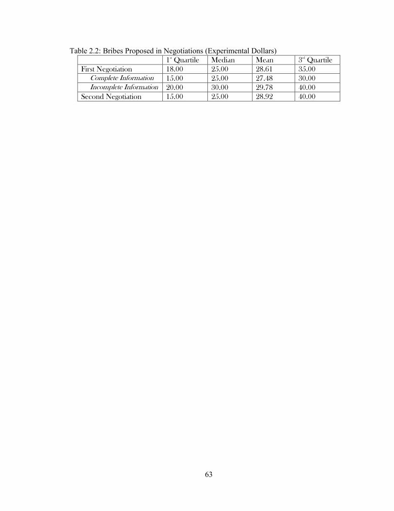
63
Table 2.2: Bribes Proposed in Negotiations (Experimental Dollars)
1st Quartile Median Mean 3
rd Quartile
First Negotiation 18.00 25.00 28.61 35.00
Complete Information 15.00 25.00 27.48 30.00 Incomplete Information 20.00 30.00 29.78 40.00
Second Negotiation 15.00 25.00 28.92 40.00

64
Table 2.3: Proposal Analysis
Dependent variable:
Proposal
(1) (2)
3-Person Treatment 3.758 0.086
(3.008) (3.305)
Incomplete Information 2.043 -1.643
(2.824) (3.691)
3-Person Treatment -2.806 -0.219
X Incomplete Information (4.240) (5.155)
Round 0.834 2.058
(1.071) (1.282)
Cycle -0.136 1.377
(2.106) (2.634)
Comprehension 0.011* 0.010
(0.007) (0.009)
Gender (1=Female) 1.502 2.594
(2.153) (2.894)
UG Major: Biology -5.992** -6.544**
(2.532) (3.141)
UG Major: ENRE 5.202 -1.378
(4.775) (4.827)
Experience -0.845* 2.050
(0.474) (1.998)
Proportion CRT Correct - -20.858**
(10.624)
Constant 124.352*** 20.293***
(4.664) (6.229)
Observations 267 153
Adjusted R2 0.035 0.025
Note: *p<0.1; **p<0.05; ***p<0.01. Fixed effects regressions reported. Robust clustered standard errors by the subject, cycle, and session are in parentheses. The unit of observation is at the subject level by session and cycle, and is considered repeated for all observations within a session and cycle. Reports a regression with the proposal made in the first negotiation as the dependent variable. Column (1) is a model including all subjects, while Column (2) reports results only using subjects who finished the CRT in time. The regression is described in Equation (10). 3-Person Group Treatment is a dummy variable for whether the subjects are in a cycle where they had 2 other members in their group. Incomplete Information is a dummy variable for whether the subjects are in a session where the available information is incomplete. Round and

65
Cycle indicate the round of the cycle and the cycle of the session in which the proposal took place. Comprehension indicates how long it took the subjects to complete the game comprehension questions at the beginning of the experiment. UG major: indicates the participant’s area of study with “Other” as the base. Experience indicates how many previous economic experiments the subject had participated in previously. Proportion CRT Correct indicates the proportion of the 3 CRT questions the participant answered correctly.

66
Table 2.4: Bribes Proposed in Complete Information Negotiations (Experimental Dollars)
1st Quartile Median Mean 3
rd Quartile
First Negotiation 15.00 25.00 27.48 30.00
2-Person 15.00 22.50 26.41 30.00 3-Person 15.75 25.00 28.55 35.00
Second Negotiation 14.75 20.00 25.47 41.25
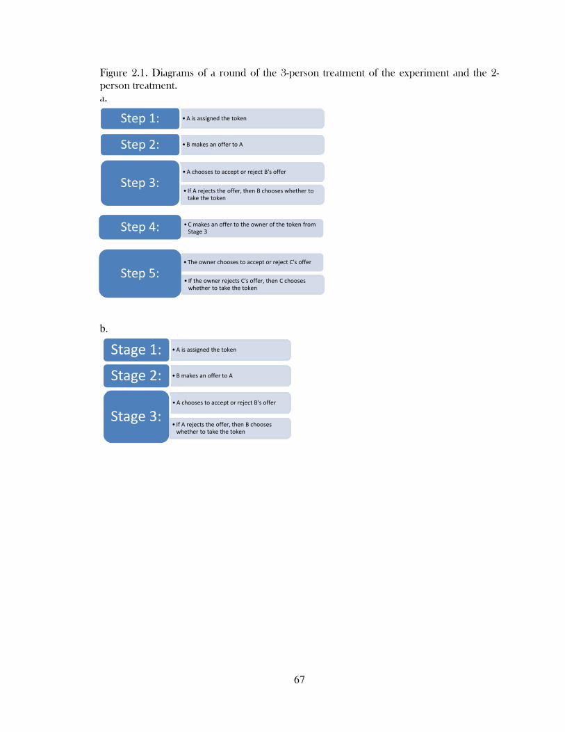
67
Figure 2.1. Diagrams of a round of the 3-person treatment of the experiment and the 2-
person treatment.
a.
b.
• A is assigned the tokenStep 1:
• B makes an offer to AStep 2:
• A chooses to accept or reject B's offer
Step 3:
• The owner chooses to accept or reject C's offer
Step 4:
• If the owner rejects C's offer, then C chooses
whether to take the token
Stage 5:
• If A rejects the offer, then B chooses whether to
take the token
Step 5:
• C makes an offer to the owner of the token from
Stage 3
• A is assigned the tokenStage 1:
• B makes an offer to AStage 2:
• A chooses to accept or reject B's offer
Stage 3:• If A rejects the offer, then B chooses
whether to take the token

68
Figure 2.2. The proportion of original owners of the token
maintaining possession of the token, by group size.

69
Figure 2.3. The proportion of original token owners maintaining
possession until the end of the first bargaining negotiation, by
information.

70
Figure 2.4. The proportion of original owners maintaining
possession of the token until the end of the first bargaining
negotiation.

71
CHAPTER 3
To be considered for submission to Journal of Environmental Economics and
Management
UNITED WE RISE, DIVIDED WE FALL:
EMPOWERING RESOURCE USERS AND LOCALIZING MANAGEMENT
by
Chris Brozyna
Environmental and Natural Resource Economics
University of Rhode Island
1 Greenhouse Road, Kingston, RI 02881, USA
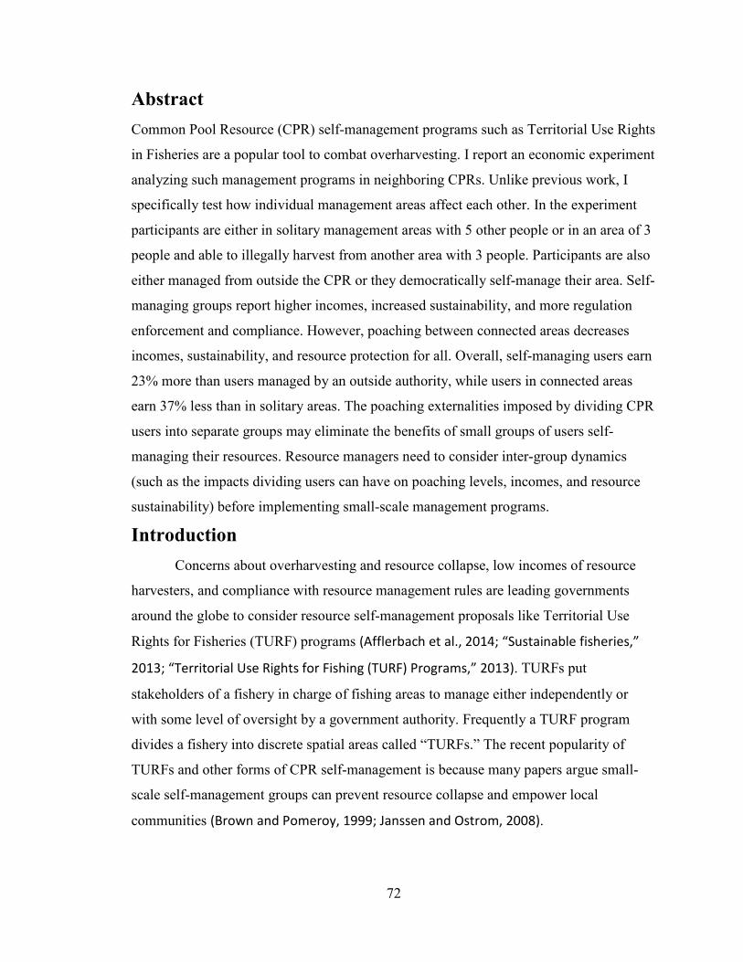
72
Abstract
Common Pool Resource (CPR) self-management programs such as Territorial Use Rights
in Fisheries are a popular tool to combat overharvesting. I report an economic experiment
analyzing such management programs in neighboring CPRs. Unlike previous work, I
specifically test how individual management areas affect each other. In the experiment
participants are either in solitary management areas with 5 other people or in an area of 3
people and able to illegally harvest from another area with 3 people. Participants are also
either managed from outside the CPR or they democratically self-manage their area. Self-
managing groups report higher incomes, increased sustainability, and more regulation
enforcement and compliance. However, poaching between connected areas decreases
incomes, sustainability, and resource protection for all. Overall, self-managing users earn
23% more than users managed by an outside authority, while users in connected areas
earn 37% less than in solitary areas. The poaching externalities imposed by dividing CPR
users into separate groups may eliminate the benefits of small groups of users self-
managing their resources. Resource managers need to consider inter-group dynamics
(such as the impacts dividing users can have on poaching levels, incomes, and resource
sustainability) before implementing small-scale management programs.
Introduction
Concerns about overharvesting and resource collapse, low incomes of resource
harvesters, and compliance with resource management rules are leading governments
around the globe to consider resource self-management proposals like Territorial Use
Rights for Fisheries (TURF) programs (Afflerbach et al., 2014; “Sustainable fisheries,”
2013; “Territorial Use Rights for Fishing (TURF) Programs,” 2013). TURFs put
stakeholders of a fishery in charge of fishing areas to manage either independently or
with some level of oversight by a government authority. Frequently a TURF program
divides a fishery into discrete spatial areas called “TURFs.” The recent popularity of
TURFs and other forms of CPR self-management is because many papers argue small-
scale self-management groups can prevent resource collapse and empower local
communities (Brown and Pomeroy, 1999; Janssen and Ostrom, 2008).
73
Though many resource management reforms involve dividing a resource into
smaller parts (Cass and Edney, 1978; Taylor, 2003), little work considers how the
resulting management groups and their users impact others. Previous research examines
how individual CPR self-management groups behave, and compares outcomes in single,
solitary government managed resources to outcomes in single, solitary self-managing
resources. But if a management program localizes management by dividing a larger
resource into smaller parts, in order to bring resource management to a more local level,
it necessarily will create multiple resource management groups. Therefore whether these
groups harm or help neighboring groups is critical. A large body of experimental research
examining competition between groups in other contexts reports a “minimal group
paradigm.” The paradigm suggests suboptimal outcomes occur because groups form out-
group biases and exhibit destructive behavior towards other groups, even when group
assignment is seemingly random or based on trivial things (Chen and Li, 2009; Diehl,
1990; Hargreaves Heap and Zizzo, 2009; Tajfel et al., 1971; Tajfel and Turner, 2001).
Kranton et al. (2018) refer to the related in-group bias as “groupiness.” Dividing fishers
into groups may initiate groupiness and minimal group paradigm behavior. Not
investigating how self-managing groups affect each other means well-intentioned
resource management proposals might hurt the very resources and communities they
mean to help.
I design a common pool resource economic experiment allowing us to determine
the effort resource users will expend to protect their resource, and whether delegating
authority over a resource to users improves profits and sustainability. In this experiment
participants are either in solitary groups of 6 users, or in groups of 3 users connected to
another group of 3 users. Players are either under a harvest management regime set by an
outside management authority, or they collectively design the management regime they
harvest under. The experiment compares the potential outcomes of an extractor managed
resource like a TURF to a classic government managed one. Unlike previous work
though it takes into account how individual management groups affect each other.
Utilizing a treatment with user groups able to extract from each other’s management
areas I examine inter-group dynamics to compare performance between larger and
smaller groups and between outside managed and self-managing groups.

74
I find dividing a resource into smaller parts leads to suboptimal outcomes while
self-managing improves outcomes. Despite comparable “rules of the game” overall,
players change their behavior after a resource is split into smaller sub-management areas
statistically significantly decreasing user incomes, resource sustainability, and increasing
violations of resource management regulations. Members of smaller connected
management areas extract 20% more overall and have incomes 37% lower than members
of larger solitary management areas. Self-managing statistically significantly increases
incomes, improves resource sustainability, and increases stewardship and resource
protection. The average income of self-managing users is 23% higher than outside
managed users and they extract 12% less. The results indicate decision-makers must be
careful and consider group competition dynamics when designing and implementing
resource management reforms.
Motivation
A particularly salient example of the dynamic described where common pool
resources are divided into smaller management areas is Territorial Use Rights for
Fisheries proposals (TURF). TURFs have recently become popular in fishery economics
to address the fisheries crisis (Poon and Bonzon, 2013). In his seminal book on the
subject, Christy explains TURF programs as giving rights to a fishery to a local
community, a community group, a co-operative of fishermen, a corporation, an
individual, etc. (Christy, 1982). Such rights include the right of exclusion, the right of
setting the harvest level, etc. Exclusion allows rents to be generated by blocking new
entrants to the fishery (who would dissipate rents) and is a critical reason for the
promotion of TURF programs. Additionally, many TURF programs divide a fishery into
discrete spatial areas called “TURFs.” Fishers, groups of fishers, or the community are
put in charge of the individual areas and manage them either independently or with some
level of oversight by the fishery’s managing authority.
Self-management proposals such as TURFs are becoming popular prescriptions
for issues in Common Pool Resources around the world, however we need more research
to make informed decisions. A major gap in the literature is the impact individual CPR
management groups have on each other. Programs dividing large resource management

75
areas to small-scale management areas to increase local control have the corollary of
creating multiple management groups in close proximity. This raises important questions.
Do members of different CPR user groups illegally harvest resources from other groups’
areas to such a degree higher overall harvests than before the resource was divided result
(González et al., 2006; San Martín et al., 2010)? Do smaller scale groups manage their
resources better than larger groups when there are other non-group users able to harvest
from their resource (McCay, 2017; Orensanz and Parma, 2010)? There is not sufficient
research on inter-CPR behaviors to answer questions about whether the benefits of small-
scale self-management programs diminish when the management groups interact with
one another.
Previous Experiments
A lack of research on how multiple CPRs interact with and affect each other
motivates this work. Economic experiments have been used extensively to examine a
range of real-world policies (Banks et al., 2003; Falk and Heckman, 2009; Ishikida et al.,
1998). While experiments examining CPRs have been around for decades (Cass and
Edney, 1978), spatial aspects like between neighboring CPRs have been neglected.
Previous research does not include multiple CPRs interacting with each other and so has
not determined their impacts on each other. Relevant experiments were absent until
recently and merely examine the differences between an outside managed resource user
group and a self-managing group. They find CPR user groups have difficulties managing
illegal extracting from outside the group and establish suboptimal management programs.
Experiments report different outcomes from communication between group members.
This experiment determines how CPR user groups affect each other, strengthens the
findings about the management regimes self-managing groups select, and adds evidence
to the debate regarding the impacts management and communication have on outcomes
(Abatayo and Lynham, 2016; Cardenas, 2000; Coleman, 2009).
Relevant experimental papers are all within recent years (Abatayo and Lynham,
2016; Arroyo-Mina and Guerrero, 2018; Chávez et al., 2018; Gallier et al., 2016; Santis
and Chávez, 2015; Wakamatsu and Anderson, 2018). While some of the experiments are
conducted in laboratories, most take place in the field. The findings of my laboratory

76
experiment are therefore more generalizable. Additionally, Chávez et al. (2018) find no
significant differences between the behavior of Chilean fishers in a field experiment and
university students in a laboratory experiment. Therefore even though my results are
more generalizable than a field experiment and will apply well to wider range of
contexts, they may still apply well to specific instances.
Unlike previous experiments, this work analyzes CPRs in the context of the entire
system of which they are a part. Most of the previous work analyzes whole CPRs
converted into a single resource-wide management program. Sometimes when self-
management systems are established the original resource is divided into smaller
management units (Aburto et al., 2013). This is to create more local management of
resource stocks. Previous work only analyzing an entire resource converting to a single
management regime misses the dynamics that occur between two management groups
when a resource is divided. This experiment fills the critical gap in the literature about the
impacts neighboring CPRs have on each other informing resource management policy
around the world.
Chávez et al. (2018) conduct an experiment using two groups of 3 users
harvesting 2 different colored locos (an abalone) in a shared fishery. The stocks of both
locos are dynamic and have a threshold where if the stock ever falls below the threshold
the management area for that colored loco will close. The participants play 5 different
treatments of the game with either no poaching (no one can extract a different colored
loco than has been assigned to them), poaching occurs (one group can harvest both types
of loco), or there is poaching but user groups decide how much surveillance (the
probability of someone illegally harvesting being caught) they will pay for to discourage
poaching. The other two treatments are there is poaching but the government will provide
a surveillance level of an 11.1% chance of catching people poaching, and finally a
treatment where the government provides an 11.1% surveillance level and the players can
augment that surveillance with additional money paid to raise the level. The authors find
the groups have difficulty deterring poaching and establish suboptimal management
regimes despite significant benefits from better regimes. Outside surveillance by the
government does deter poaching. While Chávez et al. (2018) provide an excellent study

77
of self-managing user responses to poaching, the interaction between different CPR user
groups remains unexplored.
My experiment differs from Chávez et al. (2018) because they incorporate a
dynamic stock aspect and do not include reciprocal inter-group dynamics. In their
experiment one group of participants can communicate with each other and self-manage,
while another group harvests from the main group’s resource. The asymmetric context is
specific to a resource where only one group can harvest from another and does not
analyze how different user groups affect each other back and forth. Using a TURF
program in a fishery to illustrate, Chávez et al.’s experiment examines one TURF where
outside poaching is a problem. My experiment has two TURFs connected together, a set-
up similar to some of the TURFs of Chile where neighboring groups of fishers negatively
affect each other (Orensanz and Parma, 2010; San Martín et al., 2010). In addition, their
set-up allows them to compare the outcomes from self-managing and full communication
between all the relevant fishery users to self-managing and partial communication
between all the users. Like my experiment, partial communication results from restricting
your communication to half of the users of your resource.
De Geest et al. (2017) has a similar set-up to Chávez et al. (2018), with players in
one CPR and “outsiders” able to extract from it, but uses a static extraction game with
crowding effects similar to my experiment. Like me they conduct a laboratory
experiment that does not frame the game in any context (such as a fishery), thereby
allowing their results to be more generalizable. They find group members are able to
cooperate with each other, but they are unable to control the level of extraction by
outsiders.
Previous experiments find self-managing CPR users do not select optimal
management programs. An experiment by Velez et al. (2012) examines the management
regimes users select to protect and manage their CPR. In their setting, strong enforcement
efforts (either higher penalties for illegal harvesting or higher levels of surveillance)
should theoretically always be preferred to lower levels. However in their experiment
individuals implement inefficient and weak surveillance and penalty levels. Despite
voting on important aspects of the enforcement regime and communicating with other
group members, 80% of individuals vote for the suboptimal enforcement regime with low

78
penalties and low surveillance levels. 90% of groups implement such programs.
Additionally, Janssen et al. (2013) report a field experiment where users break the rules
they choose for themselves. I contribute to the CPR self-management literature by
measuring the legal harvest limits and surveillance levels self-managing groups choose,
as well as violations of the limits groups set for themselves.
Communication and collective decision-making appear to improve outcomes in
CPR experiments, but the effect is not universal. Communication and democratic rule-
making generally improve economic outcomes (Dal Bó et al., 2010); including in fishery
contexts (del Pilar Moreno-Sánchez and Maldonado, 2010). Abatayo and Lynham (2016)
find allowing CPR users to communicate about resource management leads to
significantly lower – and more sustainable – extraction levels. Gallier et al. (2016) find
similar effects in some of their experiment sites, but in others outside management
suggestions perform better. Schmitt (2000) describes a CPR experiment where restricting
communication in a group of harvesters to a subgroup of the harvesters effectively
reduces cooperation. Velez et al. (2012) find communication does not reduce extraction
to sustainable levels. The diverse findings indicate outcomes are dependent on local
contexts and policies are not generalizable. While evidence suggests communication and
endogenous management improve economic outcomes, the impact for some CPRs in
experiments is mixed and we need more research to definitively confirm the impacts of
communication and endogenous management.
A large body of experimental research finds a minimal group paradigm and
groupiness can lead to group biases forming and suboptimal outcomes. Minimal group
paradigm argues groups form out-group biases and exhibit destructive behavior towards
other groups even when group assignment seems random or is based on trivial things
(Chen and Li, 2009; Diehl, 1990; Hargreaves Heap and Zizzo, 2009; Tajfel et al., 1971; see
Tajfel and Turner (2001) for an overview of early work on the subject). In addition,
“groupiness” appears in experiments examining group competition (Kranton et al., 2018).
Groupiness refers to a related phenomenon, where subjects become biased towards
members of their own group and against members of other groups. In my experiment,
dividing players into separate groups may initiate groupiness and minimal group
paradigm behavior.

79
Working with the experimental design of Abatayo and Lynham (2016) I can
explicitly test behavioral group concepts like “us versus them” and groupiness, concepts
not previously explored in CPR contexts but important for inter-CPR dynamics. The
major findings of Abatayo and Lynham are communication improves outcomes relative
to no communication and whether rules are exogenously imposed or endogenously
selected does not impact efficiency. In extending their work, I find “groupiness” effects
that persist regardless of any change in the ability to communicate and manage.
Model
The models of Abatayo and Lynham (2016) and Schnier (2009) guide us in
determining the impacts neighboring management areas have on each other. I have two
spatially distinct Common Pool Resources, and a constant number of agents able to
extract from the CPR system, *. (�^ identifies the extraction of user in CPR d (d = 1,2).
is the value of extracting outside the CPRs. Users cannot extract more than an
endowment, �, from both CPR 1 and CPR 2:
0 ≤ ∑ (�^ ≤ �_�
The group’s returns are a function of the total extractions from both CPRs, T ,
with each individual CPR’s return being given by E (T ). There are no spatial-linkages
between the CPRs where extractions in one directly impact the other.
Each CPR’s yield function is given by the following standard quadratic functions:
E(T) = (p − �T)T (1)
and
E_(T_) = (p_ − �_T_)T_ (2)
The first term in the parentheses shows the benefits of extracting from the group’s CPR,
the second the costs.
The private returns are shown by
F)�S &� = (� − (� − (�_) + {\;U; E(T) + {\|
U| E_(T_) (3)
where {\]U] is ’s share in the total extraction from CPR d. Users are profit-maximizers who
cannot extract more from both CPRs than their endowment. Extracting from the CPR

80
earns more than the outside option, , initially, but as T grows extraction eventually
becomes less profitable. With identical �, , and E , we can find the following symmetric
Nash Equilibria:
(�∗ = (~;�4)(�Q)V;(�Q)| (4)
and
(�_∗ = (~|�4)(�Q)V|(�Q)| (5)
In my experiment design both CPRs have identical parameters so p = p_ = p
and � = �_ = �. With = 0, we can simplify Equations (4) and (5) to:
(�∗ = ~V(�Q) (6)
and
(�_∗ = ~V(�Q) (7)
With * members in a group, the total Symmetric Nash Equilibrium extraction in each
CPR is:
T∗ = X ��Q[ ~
V (8)
The socially optimal level of extraction maximizes profits for the entire group. To
find the socially optimal level chosen by a Social Planner, we use the objective function:
max{U;U|} ⋯ (*� − T − T_) + E(T) + E_(T_) (9)
given aggregate extractions cannot exceed aggregate endowments (∑ ∑ (�^ ≤ *�_���� ).
The socially optimal extractions for the group are:
T�� = _V|(~;�4)�V;V| (10)
and
T_�� = _V;(~|�4)�V;V| (11)
With = 0, p = p_ = p, and � = �_ = � we get:
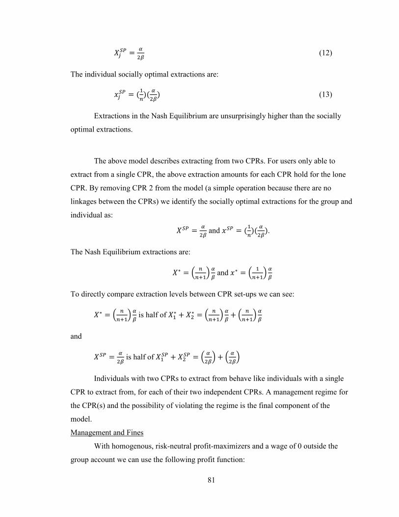
81
T�� = ~_V (12)
The individual socially optimal extractions are:
(�� = (�)( ~
_V) (13)
Extractions in the Nash Equilibrium are unsurprisingly higher than the socially
optimal extractions.
The above model describes extracting from two CPRs. For users only able to
extract from a single CPR, the above extraction amounts for each CPR hold for the lone
CPR. By removing CPR 2 from the model (a simple operation because there are no
linkages between the CPRs) we identify the socially optimal extractions for the group and
individual as:
T�� = ~_V and (�� = (
�)( ~_V).
The Nash Equilibrium extractions are:
T∗ = X ��Q[ ~
V and (∗ = X �Q[ ~
V To directly compare extraction levels between CPR set-ups we can see:
T∗ = X ��Q[ ~
V is half of T∗ + T_∗ = X ��Q[ ~
V + X ��Q[ ~
V
and
T�� = ~_V is half of T�� + T_�� = X ~
_V[ + X ~_V[
Individuals with two CPRs to extract from behave like individuals with a single
CPR to extract from, for each of their two independent CPRs. A management regime for
the CPR(s) and the possibility of violating the regime is the final component of the
model.
Management and Fines
With homogenous, risk-neutral profit-maximizers and a wage of 0 outside the
group account we can use the following profit function:

82
F)�S &^ = α( − ( q�T r
In reality users of many CPRs, and by definition all TURFs, have the ability to
enact management regimes to create and enforce limits on extractions. Stronger
enforcement of the extraction rules costs users more money than weaker enforcement of
regulations so the profit function for CPR users becomes:
F)�S &^ = α( − ( q�T r − �!*!t�'�*& ��,&^
�!*!t�'�*& ��,& represents the cost to each player to provide the given level of
management for their group’s CPR.
Finally, I also allow for individual violations of account extraction regulations to
be punishable by a fine on the individual. Since extracting benefits you privately and the
costs are shared with everyone else extracting from the CPR, there is an individual
incentive to extract more. The socially optimal level balances the benefits and costs for
the group, but cheating by extracting more while everyone else cooperates and extracts at
the socially optimal level earns you more money. It is therefore in your personal interest
to extract more while everyone else extracts at the lower level. The fine in the experiment
is set to the profit a user gains by extracting at the optimal cheating level, (�,��, when
everyone else in their group extracts from CPR^ at the socially optimal level, (��,^�� .
E *��,^ = F)�S &�,^q(�,��q(��,^�� r, (��,^�� r − F)�S &�,^((�,^�� , (��,^�� ) (14)
where (�,��q(��,^�� r = ~�(��)V{:\,]��_V
for user . (�,��q(��,^�� r is found by solving as we have above, but without symmetric actions
by all the agents.
F)�S &�,^ = α(�,^ − (�,^q�T�,^r
= α(�,^ − (�,^ X�(�,^ + � �(��,^�� [
�F)�S &�,^�(�,^ = α(�,^ − 2�(�,^ + � �(��,^�� = 0
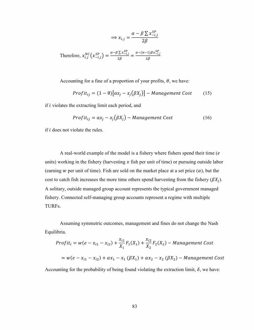
83
⟹ (�,^ = p − � ∑ (��,^��2�
Therefore, (�,��q(��,^�� r = ~�V ∑ {:\,]��_V = ~�(��)V{:\,]��
_V
Accounting for a fine of a proportion of your profits, �, we have:
F)�S &�^ = (1 − θ)hα( − ( q�T ri − �!*!t�'�*& ��,& (15)
if violates the extracting limit each period, and
F)�S &�^ = α( − ( q�T r − �!*!t�'�*& ��,& (16)
if does not violate the rules.
A real-world example of the model is a fishery where fishers spend their time (�
units) working in the fishery (harvesting ( fish per unit of time) or pursuing outside labor
(earning per unit of time). Fish are sold on the market place at a set price (p), but the
cost to catch fish increases the more time others spend harvesting from the fishery (�T ).
A solitary, outside managed group account represents the typical government managed
fishery. Connected self-managing group accounts represent a regime with multiple
TURFs.
Assuming symmetric outcomes, management and fines do not change the Nash
Equilibria.
F)�S &� = (� − (� − (�_) + (�T E(T) + (�_T_ E_(T_) − �!*!t�'�*& ��,&
= (� − (� − (�_) + p( − ( (�T) + p(_ − (_ (�T_) − �!*!t�'�*& ��,&
Accounting for the probability of being found violating the extraction limit, c, we have:

84
F)�S &� = (� − (� − (�_) + (1 − c)hp(�, − (�,(�T)i + (c)=p(�, − (�,(�T)](1− θ) + (1 − c)=p(�,_ − (�,_(�T_)] + (c)=p(�,_ − (�,_(�T_)](1 − θ)− �!*!t�'�*& ��,&
If ( is below the extracting limit for the CPR, there is no risk of a fine and
�������\�{; is unaffected by the presence of management.
(∗ = � 1* + 1� p
�
If the socially optimal extraction is below the limit for the CPR, there is no risk of
a fine and the socially optimal extraction level is the same with management as without
management.
(�� = (1*)( p
2�)
The presence of a management regime punishing other group extracting affects
�������\�{| . But the effect does not impact your optimal other group extraction. The other
group extraction amount from before the introduction of management is still optimal. �F)�S &��(_ = − + (1 − c)=p − 2(_� − (* − 1)(_�]
+ (c)=p − 2(_� − (* − 1)(_�](1 − θ)
For both solitary groups and connected groups where the socially optimal
extraction is below the limit, the presence of management and fines do not impact the
optimal harvest.
Without management (∗ = X �Q[ ~
V and (�� = (�)( ~
_V) in a solitary group’s
account, or in each group account for connected groups. Under management, we derive
the same result as without management, but multiplied by a constant. The constant falls
away when we identify the Nash Equilibrium and socially optimal extraction levels.
�F)�S &��( = − + (1 − c)=p − 2(� − (* − 1)(�] + (c)=p − 2(�− (* − 1)(�](1 − θ)

85
= =1 − θc]=p − (* + 1)(�] = 0
⇒ =1 − θc]p = =1 − θc]=(* + 1)(�] ⇒ (∗ = � 1
* + 1� p�
The presence of management does not impact the Nash Equilibrium extraction
level. Management also does not change the socially optimal extraction level.
�F)�S &��( = − + (1 − c)=p − 2*(�] + (c)=p − 2*(�](1 − θ)
= =1 − θc]=p − 2*(�] = 0
⇒ =1 − θc]p = =1 − θc]=2*(�] ⇒ (�� = �1
*� p2�
Experimental Design
The experiment is a common pool resource game similar to Abatayo and Lynham
(2016). Each Period the group members decide how many tokens to extract from a
“group account” CPR they share with either 2 or 5 other people. They are given an
endowment to spend each Period. The endowment may be spent either extracting tokens
or on the outside activity (the activity paying a set amount per unit in the model). I set the
outside wage, , to zero, so players only earn Experimental Dollars from the tokens they
extract. The design is a classic 2x2 experiment. The control of players over setting
harvest limits and enforcement of those limits is the within subject treatment. Whether
the group account is split into two connected sub-accounts or kept together in a solitary
account is the between subject treatment.
The profit earned each Period is a constant individual payoff from each token
extracted minus a term accounting for total extraction from the account in the Period and
the user’s share of the total. The extraction of each individual is simplified to ( and total

86
extraction by everyone in the group account becomes T (= ∑ (�,^). The strategy set for
users is between 0 and � in each Period.
One half of experiment Sessions have participants play the game in solitary
groups with a large group account shared by 6 people. The other half of Sessions have
players in groups of 3 people who share smaller accounts and can interact with the group
account of another group of 3 people. Group members can only extract tokens from their
account in the solitary groups. Players are able to extract a certain number of tokens
legally from their group’s account, but they can also illegally extract above the legal
limit. Players in the connected group treatment have the additional option to extract from
the other group’s account illegally. I call the act of extracting tokens from the other
group’s account “poaching.”
Specifying the model’s parameters allows us to assign numerical values to the
equilibria. � = 20, = 0, and p = 15. � = 0.25 in connected groups and � = 0.125 in
solitary groups. � is half as large in solitary groups as in connected groups to reflect the
greater relative impact the removal of a token has in a smaller account. The 6-person
group set-up represents an entire solitary fishery and the two 3-person group set-up
represents a larger fishery divided into two sub-fisheries. You can imagine removing one
fish in an ecosystem encompassing half of a fishery being twice as impactful to the other
fishers there as it would be to the fishers in a whole larger fishery; hence the difference in
�s. With * = 6 we can fully parameterize the functions and find the equilibria for the
experiment.
Without considering management, simplifying the general Nash Equilibrium
equations of the model, (6) and (7), leads to (�∗ = 8.57 and (�_∗ = 8.57 together totaling
17.14 tokens. The results suggest a strategy of extracting 8.57 tokens from your group’s
account and poaching 8.57 from the other group’s account.
For solitary groups, � = 0.125, and there is only one account. We therefore
find (∗ = 17.14.
Total group extractions at the Nash level are T∗ = 102.86 for the solitary group
and 51.43 for each CPR in the connected group setting (102.86 total).

87
Parameterizing the socially optimal extractions for the connected group accounts
(Equations (12) and (13)) gives T�� = 5 and T_�� = 5 leading to a total (�� = 10. T�� =60.
For solitary groups with 1 account we have (�� = 10, also with T�� = 60.
Both group size treatments have the same socially optimal and Symmetric Nash
Equilibrium extraction levels. Solitary and connected group members each extract 17.14
tokens in total at the Nash Equilibrium. The socially optimal individual extraction level is
10 tokens for both connected and solitary groups.
The socially optimal total extraction, T��, is 60 tokens (each connected group
account has a total socially optimal extraction of 30, and both together is a total socially
optimal extraction of 60 tokens). Players earn 75 Experimental Dollars extracting at the
socially optimal level.
Total Nash Equilibrium extraction is T∗ = 102.86 (again, summing up the
extractions of two connected groups of 3 people or a single solitary group of 6 people).
Players earn 36.75 Experimental Dollars extracting at the Nash level. Nash extraction for
connected groups is identical to solitary groups because both group treatments occupy
systems with 6 users and utilize accounts with �s proportional to their fraction of the
overall system.
Management and Fines
The next aspect of the experiment reflects the presence of externally provided
resource management or the self-provision of management. In half of a Session’s
treatments the management regime is set outside the group by the experimenter
(representing the role of the government in a typical real-world fishery). The outside
management sets a limit, or “cap,” on how many tokens each individual user can legally
extract from their group account each Period. In a TURF context, the cap represents a
fishing limit. Anything you extract above your cap is considered illegal and there is a
percentage chance your illegal extracting will be discovered. The chance of being found
is the “level of surveillance.” Managed users pay a set fee each Period to cover the costs
of the regime and are told the cap and level of surveillance at the start of each Period.
Self-managing groups democratically choose the cap and the level of surveillance before
making extraction decisions.

88
In-game violations of account extraction regulations are punishable by a fine.
Extracting at the optimal cheating level while everyone else cooperates and extracts at the
socially optimal level earns you the highest amount of Experimental Dollars. The
model’s fine is set to the profit a user gains by extracting at the optimal cheating level,
(�,��, when everyone else in their group extracts at the socially optimal level, Equation
(14).
Using the parameters set for the experiment, F)�S &�,^q(�,��q(��,^�� r, (��,^�� r = 100
and therefore E *��,^ = 25% (100-75). Since users are never able to change the size of
the fine, it is never more than 25 Experimental Dollars. Since there is no 100% possibility
of being discovered violating the regulations, only being fined the profit from violating is
not enough to deter rational users.5 If self-managing users choose the maximum level of
surveillance available, 50%, the fine of 25% of your profits for breaking the management
rules is too low to effectively deter poaching. Thus we have weak enforcement of the
rules. I create a regime with weak enforcement because that is the norm in most CPRs
including fisheries (Sutinen et al., 1990). Other experiments follow similar procedures
(Abatayo and Lynham, 2016; Chávez et al., 2018).
Accounting for the fine, we have the following profit functions for extracting
from your group’s CPR: F)�S &^ = 0.75h15( − ( q�T ri − �!*!t�'�*& ��,&^ if a
user is found violating the cap, and F)�S &^ = 15( − ( q�T r − �!*!t�'�*& ��,&^ if
a user extracts below or at the extraction cap.
Under the outside management regime, the socially optimal extraction strategy is
to extract 10 tokens from your own group’s account. Following the strategy maximizes
total wealth for the group, but it is not an equilibrium as it is always better for the
individual to harvest 11 tokens than 10. With a management regime consisting of a cap of
12 and a surveillance level of 10%, the total socially optimal extraction amount for an
individual, (�� = 10, is below the cap. Each token you extract from the other account is
5 The fine is not large enough because the maximum you can earn from cheating is 25 Experimental
Dollars, the fine will only equal 25 Experimental Dollars when you are caught optimally cheating and
everyone else cooperates. Additionally, taking into account the chance of being fined, the expected fine
will always be lower than 25 Experimental Dollars so a risk neutral user would not be deterred by the fine.

89
at a 10% risk of being fined. Therefore the expected utility from a token harvested from
your group’s account (with zero chance of incurring a fine) is higher and you will extract
all 10 tokens from your group’s account.
0.10 ¡�F)�S &¢�(¢ £ (0.75) + (0.90) ¡�F)�S &¢�(¢ £ ≤ ¤�F)�S &^�( ¥ ℎ�* ( ≤ 12
The socially optimal harvest level is the same under management as it is without.
The management regulations merely adjust where individuals harvest their 10 tokens
between CPRs in the connected setting. The socially optimal harvest is also below the
cap for the solitary groups (12) and so management has no effect on the socially optimal
harvest amount in solitary settings.
Assuming symmetric outcomes, we can see that management and fines do not
affect the Nash Equilibrium. With a Nash Equilibrium above the cap, players extracting
at the Nash level are at risk of being fined.
Under outside management, the Nash Equilibrium harvest in the solitary groups is
the same as we found without considering management, ( = 17.14.
Under outside management, the Nash Equilibrium spatial distribution of token
extraction between connected groups is the same as without the management program.
The distribution of tokens without management is 8.57 in each account, an amount below
the own-group harvest cap of 12. Therefore the cap does not impact your extraction from
your own group account. Meanwhile, extracting 8.57 tokens from the other group’s
account maximizes your discounted profit function without management and fines. The
possibility of being fined for extracting from the other group merely acts as a constant
multiplied by the profit function. Players still extract at the same level in the Nash
Equilibrium. Therefore extractions from the two accounts remain symmetric between
them at the same levels as they were when there was no management regime.
The Nash Equilibrium for both CPRs is the same under management as it is
without management. �������\
�{; is unaffected by the presence of management when your
own group extraction is below the harvest cap. So the same own group extraction is
optimal, ( = 8.57. �������\
�{| is affected by the presence of management. But the effect
does not change the harvest level we derive, (_ = 8.57.
90
The presence of management and fines do not impact the Nash Equilibrium.
Solitary group members harvest the same number of tokens under management as they
do without management. Similarly, connected group members at the Nash Equilibrium
harvest the same number of tokens from their group and from the other group under
management as they do without management. Table 3.I summarizes the theoretical
predictions. Since solitary groups and connected groups harvest the same overall amounts
as each other in the Nash Equilibrium and have identical socially optimal harvest levels,
and management and fines do not introduce any differences, we should not see any
differences in harvests between solitary groups and connected groups. Behaviorally based
concepts and explanations such as groupiness would best explain any differences in
harvests.
Hypotheses
The experimental design allows me to test the hypotheses that group division and
self-managing will impact outcomes. Impacts will suggest the presence of behavioral
factors CPR management proposals need to consider before dividing a resource into
separate management entities.
In the absence of such behavioral factors, there should be no difference in
extractions between a large united group and two smaller divided groups. Theory, the
model, and the specific parameterization of the experiment predict there will be no
differences. Both group set-ups have a socially optimal extraction amount of 10 tokens
per individual and a Nash Equilibrium amount of 17.14 tokens per individual.
Hypothesis 1: Cooperative and sustainable behavior of
connected groups will be statistically significantly
different from behavior of solitary groups.
I test Hypothesis 1 using the number of tokens harvested, players’ profits,
management regimes (the levels of surveillance and extraction caps set), and regulation
violations (the frequency and magnitude of violations of caps).
Despite predictions by models of group decision-making, small-scale self-
management proposals rely on behavioral factors like users feeling more invested in

91
locally made decisions than decisions made at more distant levels. Because individuals in
smaller group sizes feel more empowered to impact their outcomes (Agrawal and Goyal,
2001), the smaller connected groups may feel the regulations and outcomes are more
responsive to group members and outperform larger solitary groups. Poaching activity
from outside the group may mitigate the effect by introducing a force in the connected
groups’ environments they do not feel able to control. Users who do not feel able to have
an impact might not behave in a socially optimal way and might behave selfishly.
However, the poachers merely replace other group members from the 6-person solitary
group set-up. Players in connected groups should still feel more empowered in their
smaller group. Dividing groups allows me to explicitly test the idea of “groupiness” by
measuring cooperative behavior towards own-group players and non-cooperative
behavior towards other-group players. The experiment directly compares predictions of
group theory and behavioral precepts of small-scale self-management theories in
describing observed behavior.
Previous work regarding endogenous enforcement decisions and management in
CPR experiments indicates endogenously determined rules are more effective and
followed more regularly than exogenously imposed rules attempting to achieve efficient
management. Villena and Chavez (2005) go so far as to suggest CPRs will be unable to
avoid overharvesting without endogenous regulation. Previous research indicates I will
be unable to reject the hypothesis below.
Hypothesis 2: Self-managing groups will report
statistically significantly different measures of
cooperative and sustainable behavior from outside
managed groups.
I will test Hypothesis 2 using the numbers of tokens harvested, the players’
profits, the levels of surveillance and harvest caps set, and the frequency and magnitude
of violations of set harvest caps. I expect self-managing groups to show lower token
extraction levels, higher profits, higher levels of surveillance and lower harvest caps set
than by outside management, and lower frequencies and magnitudes of regulation
violations.

92
Experimental Procedures
A total of 108 undergraduate and graduate students were recruited at a public
university in the United States and paid based on their performance in the game.6
Participants played two Cycles of the game in the fall of 2018. A Cycle is 10 Periods of
the same CPR game under the same management regime (outside management or self-
managing). To prevent order effects the order participants play management treatments is
randomized. Cycle describes whether subjects are in the first treatment they play or the
second. The experiment was conducted using the software z-Tree (Fischbacher, 2007).
Participants received a show-up fee of $10 and the average payout at the end of the game
was $18.92. The payout was based on each Experimental Dollar earned by participants
being worth $0.01 USD. 56.25% of participants were female, the average grade level of
the students was a junior, and most participants had not previously participated in an
economic experiment. I used previous experiments (Abatayo and Lynham (2016), De
Geest et al. (2017), Chávez et al. (2018) among others) as a guide to determine the
sample size needed in this experiment. A power analysis was not completed prior to
running the experiment to determine the sample size for between subject and within
subject samples.
To begin their experiment Session, each player discovers whether they are in a
solitary group of 6 people or in a connected group of 3 people. The players answer a short
demographic survey (their major, gender, experience with economic experiments, etc.),
complete 3 questions confirming their comprehension of the game, and begin playing the
first Cycle. Participants play both management treatment Cycles (in random order) and
6 A total of 120 students were recruited but 2 participants left their Sessions a couple Periods before the
end. They left descriptions of their strategies and activities in the game up to their departure, and gave
instructions on how the experimenter should play the game from their computer after they left. These
instructions were detailed and gameplay continued seemingly uninterrupted for the final Periods. I
remove the subjects’ data and the data from the rest of the members of their solitary group or connected
groups (for the entire Session) from the analysis due to concerns regarding validity. I therefore report
findings from the remaining 108 players. Including the full sample gives comparable results to what I
report, but with higher statistical power. I did not run an additional session to reach 120 participants
because the findings already exceeded the minimum differences the experiment had been designed to
capture.

93
finally are paid for participating in the experiment. All decisions made in the game are
anonymous.7
When extracting in the outside management treatments, players are told they can
extract up to and including 12 tokens from their group’s account legally. If you harvest
above the “cap,” there is a 10% chance the computer will find you harvesting above the
cap and will assess you a penalty of 25% of your profits. The cap and percentage chance
of being fined were chosen based on the methods and results found in Abatayo and
Lynham (2016). Both my experiment and theirs select them because the set cap is just
above the social optimal level (10 tokens) and the level of surveillance (10%) is too small
to discourage uncooperative behavior. Furthermore, the cap and surveillance level are
almost identical to the average cap and surveillance level participants in an unpaid pilot
Session chose. In a similar experiment, the level of surveillance is set at 11.1% for almost
identical reasons to mine (Chávez et al., 2018).
In the self-managing treatments, before the players make any decisions about
harvesting, they discuss and vote on the management regime. Each Period they first
communicate with their group members during a 2 minute chat. A chat feature in the z-
tree software allows players to type and send instant messages anonymously. After 2
minutes they see a screen where they vote on the cap for the Period. The median vote
from the group is chosen to be the cap. After voting on the cap concludes, the players see
a similar screen where they vote for the level of surveillance for the Period. They choose
a level from 0-50% in 10% increments and the median vote from the group is the level
chosen. The surveillance level determines the percentage chance the computer will
discover a group member exceeding the cap, or someone from the other group who is
poaching from your group’s account. If the computer discovers you, you are fined 25% of
your profits. The fines collected do not go to the players but go to the computer. Each
level of surveillance has a cost that is assessed to each player (Table 3.II). The levels
increase in cost so there is realistic diminishing returns from surveillance. The
endogenous management construction is the same as Abatayo and Lynham (2016).
The levels of surveillance self-managing players can select are chosen based on
the levels in Abatayo and Lynham (2016). The range allows me to examine cooperation
7 The order of the Session elements was set based on feedback from a pilot Session.

94
and management decisions in settings where enforcement is weak. 0% is the minimum an
account could be surveilled, 50% is the maximum percentage chance to intercept
someone illegally harvesting. 50% is the most real-world TURFs could expect to surveil,
fisheries are almost always at an even lower surveillance level (Sutinen and Kuperan,
1999). In addition to low surveillance levels, many CPRs have relatively small fines for
violations (Cardenas et al., 2000).
In both outside management and self-managing treatments the penalty for
violating regulations is confiscating 25% of an illegal harvester’s profits. The penalty in
the experiment is based on the value in Abatayo and Lynham (2016), reflects the
relatively low penalties most fishery managers render, and represents penalties which are
too low to effectively discourage illegal fishing (Sutinen et al., 1990).
Players in the self-managing solitary groups have full communication between all
the relevant resource users. Self-managing connected groups have only partial
communication between all the relevant users (players can communicate with their own
group members, but not with members of the other group who can poach from their
account).
This experiment design enables examination of local user management –
specifically self-management, devolving the level of decision-making, and inter-CPR
aspects – on profitability, sustainability, responsibility, and criminality.
Results
Self-managing groups outperform outside managed groups and solitary groups
outperform connected groups. For each dependent variable I report the findings of the
preferred random effects regression model, or logistic regression model for a specific
aspect of rule violations.8 Comparing to outside managed players, self-managing players
harvest fewer tokens (thus increasing their incomes) and choose higher levels of
surveillance to catch illegal harvesting than the set outside management regime.
Connected group players harvest more tokens than solitary group players resulting in
lower incomes for them. Solitary group members harvest more tokens from their own
8 Previous experimental research uses random effects rather than fixed effects (Abatayo and Lynham,
2016; Chávez et al., 2018) and diagnostics indicate random effects are better in this context. Running
identical models under fixed effects gives very similar coefficients on the variables of interest.

95
group account on average than connected players (13.99 versus 11.31 tokens) and extract
3.31 tokens over the cap when they break the cap. Cap breakers in connected groups only
take 1.86 tokens over on average. However, because connected group members also
poach, they extract more tokens overall than solitary groups members (16.81 tokens
versus 13.99 tokens). Additionally, self-managing solitary groups choose lower harvest
cap management regimes. Inter-CPR effects are larger than the effects from allowing
players to communicate and self-manage. Regressions support the patterns in Table 3.III.
Mann-Whitney statistical tests find significant differences in means between
treatment groups. I find the differences in mean total harvest, own group extraction, cap
selection, percentage of group exceeding the cap, amount above the cap extracted, and
profit between group size treatments and management treatments are statistically
significant at the 1% level using a Mann-Whitney two sample statistic test. Differences in
mean surveillance levels chosen and poaching amounts are not statistically significant.
My larger solitary groups exhibit a stronger impact from self-managing and
communicating than Abatayo and Lynham’s smaller groups report. The average
extraction in Abatayo and Lynham’s 3-person solitary groups is 12.03 for self-managing
able to communicate and 13.64 for outside managed groups unable to communicate.9 The
average extraction in my self-managing solitary groups of 6 people is 12.76 (0.22) tokens
a Period and 15.22 (0.21) for outside managed solitary groups. Larger solitary groups
experience a greater positive impact from being able to communicate and set their own
management regime.
If we only examine the harvest behavior within our outside-managed groups, we
find a difference in average total harvests that is unrelated to the communication effect
Abatayo and Lynham describe. Outside-managed connected groups harvest 16.12 tokens
but outside-managed solitary groups harvest 12.76 tokens.
9 In their paper, Abatayo and Lynham divide their results by Session Cycle. The per-Cycle average token
extractions they report are 13.21 (0.64) in the first Cycle and 10.84 (0.37) in the second Cycle for
endogenous management. For exogenous management they are 13.05 (0.65) and 13.26 (0.64) for rules
generated by another group unable to communicate, and 13.58 (0.38) and 14.68 (0.48) for rules
generated by another group able to communicate.

96
Users’ Incomes
The profits of players in the solitary groups are consistently larger than those in
the connected groups. The difference between group-sizes is substantial. Players in
connected groups earn 20.28 Experimental Dollars less each Period than members of
solitary groups (Figure 3.1).
Figure 3.2 indicates player profits in the groups able to collectively decide upon
the management for their resource are higher overall than for outside managed players.
Table 3.IV identifies a temporal aspect where outside managed players exhibit decreasing
incomes over time. Each Period of the game outside managed players earn 1.08
Experimental Dollars less than the previous Period (Table 3.IV Column (3)).10 The
pattern holds over all the Periods participants play after the first Period, self-managing
players always earn more than outside managed players. But while the overall effect is
economically significant the difference in incomes is not as large as the difference
between connected and solitary groups (16.64 Experimental Dollars each Period in the
preferred model, Table 3.IV Column (3)).
Players earn 4.92 fewer Experimental Dollars in the second Cycle than in the first.
Each experiment a player previously played leads to an additional 3.76 Experimental
Dollars.
Harvest Behavior
Group size significantly effects harvest behavior, and individuals in self-
managing groups harvest less each Period while outside managed individuals harvest
more each Period. Poaching leads to higher total harvests, and since poaching only occurs
for connected groups it drives the difference in harvests between the group treatments.
Table 3.V gives a breakdown of the important covariates affecting harvesting.
Table 3.V Column (3) shows solitary group members extract more from their
group account, supporting the findings of Table 3.III. Though there is a significant effect
in Column (1), at first glance it may appear there is no difference between the group
treatments in Columns (2) and (3). However, looking at the coefficient on Poaching, we
see the driving force behind the significant, positive coefficient on Solitary Group in
10 Self-managing players earn an additional 0.43 Experimental Dollars each period, but the amount is not
statistically significantly different from 0.

97
Column (1). In a connected group you can poach from the other group’s account. There is
nowhere else to extract from in the solitary groups. Poaching acts as an escape valve for
own group extraction, though previous poaching and poaching by the other group raise
you own group extraction a little. Poaching necessarily externalizes token extraction,
giving the appearance of higher harvests in solitary groups. The total tokens solitary
groups harvest may not necessarily be larger than the totals connected groups harvest if
we take poaching into account, as I do in Columns (6)-(8). Meanwhile, self-managing
decreases extractions from your group’s account each Period (Column (3)). Finally, more
experience with experiments increases the number of tokens you extract.
Table 3.V Column (5) indicates the amount the other group poached from your
group’s account, the level of surveillance for your group account, and time raise your
extraction from the other group’s account. Theory predicts high poaching levels will
encourage higher extractions from your own account and from the other group’s account.
Theoretically, violations by others leads to more violations by you because compliance
with rules is frequently a result of you believing other people will comply as well (Young,
1979). Communicating and voting with other group members about management could
increase your belief group members will cooperate. We see this in own group extracting
behavior where self-managing leads to lower harvests over time. While you could just
extract less from your account and poach more from the other account, we see no pattern
of self-managing impacting levels of poaching. However, higher poaching by the other
group leads to you poaching more. Another interesting finding is the higher the
probability of being caught breaking your group’s harvest cap, the more you extract from
the other group. Changing accounts to target for illegal extracting suggests higher
surveillance levels displace extraction behavior spatially between accounts. Finally, your
experience with other economic experiments lowers the amount you poach.
Combining own-group and out-group harvest, connected groups harvest more
tokens overall than solitary groups while outside managed groups harvest 0.099 more
tokens each Period and self-managing groups harvest 0.179 fewer tokens each Period
than the last. Both management groups harvest statistically similar levels initially (Table
3.V Column (8)). Because solitary groups do not have another group’s account to extract
from – like connected groups do – a more accurate measure than own group extraction is

98
the total number of tokens you harvest. Total harvest is your extraction from your solitary
group’s account, or the sum of your extraction from your group’s account and another
group’s account for connected group members. Smaller groups lead to more cooperative
behavior with your group members (lower own group harvesting). But the cooperation is
subsidized by non-cooperative behavior towards the other group (more poaching), fitting
the idea of groupiness. The result is higher overall levels of harvesting.
Figures 3.3 and 3.4 illustrate the overall treatment effects the harvest regressions
identify. They show the average total harvest of solitary groups is 2.82 tokens lower than
the average in connected groups and self-managing reduces average token harvest by
1.92 tokens overall.
Management and Enforcement
Table 3.VI indicates self-managing groups choose higher surveillance levels than
the suboptimal level the government provides. Solitary groups choose caps 1.42 tokens
lower than connected groups on average (Table 3.III). Groups in the second Cycle choose
caps 1.806 higher than groups in the first Cycle and each additional experiment the group
has previously played on average increases the cap by 2.382 (Table 3.VI Column (2)).
The number of tokens the other group previously poached from your account lowers the
cap you choose, indicating groups attempt to choose optimal caps in the face of external
extracting. The higher the surveillance level the other group chose the previous Period,
the higher the surveillance level your group chooses (Column (5)). A 10% increase in the
other group’s surveillance level leads to a 2.69% increase in the surveillance your group
chooses the next Period. Players may worry the other group’s higher surveillance will
cause members of their group to harvest more from their own account next Period
because they anticipate the surveillance will be too high next Period to safely poach.
Therefore a higher surveillance level by the other group encourages your group to set a
higher surveillance rate to prevent a rush of own-group extracting. The average
surveillance level all self-managing groups choose is 18.34% (Table 3.III). 10% is the
level outside management provides. T-tests confirm that self-managing groups are
statistically different from outside management in terms of the caps and levels of
surveillance they choose (Table 3.III).

99
Comparing my self-managing, solitary, 6-person groups to Abatayo and
Lynham’s self-managing, solitary, 3-person groups, I find my solitary groups choose
comparable harvest caps, but significantly higher surveillance levels. The groups in
Abatayo and Lynham choose an average cap of 10.30 (0.58) and a surveillance level of
5.13% (2.45). My groups choose a cap of 10.49 (0.21) and a surveillance level of 17.70%
(1.12) (Table 3.III).
Illegal Activity
Summary statistics indicate solitary group members are more likely to extract
more from the group account than the cap (Table 3.III). 16% more members of solitary
groups violate their group’s cap than in connected groups (a difference of about 1
member violating in connected groups versus 3 members in solitary groups) (Figure 3.5).
Besides more frequently violating the cap, they extract statistically significantly more
tokens (1.45 more) when they break the cap than connected group members do when they
break the cap (Table 3.III). This is unsurprising given connected groups can use their
effort to extract from another group’s account instead of their own.
However, solitary groups may not necessarily be more felonious; “groupiness”
may explain the findings. In Table 3.VII solitary group members appear to show lower
levels of harvest cap violations than connected group members. Poaching behavior drives
the difference between the coefficients on Solitary Group in Table 3.VII (Columns (2)
and (3)) and the summary statistics. The more you poach the less likely you are to break
the cap and when you do you harvest less above the cap. Connected players poach an
average of 5.5 tokens. Given the coefficient on Poaching (Column (3)), the effect from
poaching more than offsets the effect from Solitary Group indicating solitary members
violate their cap less frequently. The pattern suggests poaching is a substitute for own-
group harvesting (the coefficient on Solitary Group in Column (1) supports the idea by
indicating Solitary Groups violate their cap more frequently when poaching is not
controlled for), illustrating the concept of “groupiness.” Smaller group sizes in the
connected treatment lead to more cooperative behavior within your own group,
cooperation that is subsidized by non-cooperative behavior toward the other group. In
fact, because poaching significantly explains whether you violate your own group’s cap,
my results directly follow the idea of groupiness.

100
Without considering interaction effects, self-managing group members break the
cap less, and when they do they break it to a smaller extent (Columns (2) and (5)). But
when interaction effects are considered, being involved in management decision-making
has no impact on your likelihood to violate the cap you just voted on (Column (3)).
Unsurprisingly, higher caps lead to fewer and smaller violations of the cap. More
individuals break the cap in the second Cycle than in the first, and when they do they
harvest more than cap breakers in the first Cycle. Higher levels of surveillance lead to
fewer tokens taken above the cap, and discourage players from breaking the cap without
considering interactions (Columns (2) and (5)).
The proportion of players breaking their group’s harvest cap and the amount they
extract above the cap are affected differently by the demographic covariates collected
(Columns (3) and (6)). Environmental Economics majors extract statistically fewer
tokens above the cap when they break the cap. Each additional experiment you have
participated in previously increases how many tokens you harvest above the cap.
Self-managing a shared common pool resource improves measures of user
incomes, resource extraction amounts, and the management programs enacted while
dividing a shared resource and its users into smaller groups lowers such measures. Self-
managing groups have lower token harvest levels, greater levels of rule enforcement, and
higher profits. Solitary group accounts experience lower harvest levels, their members
choose more efficient management parameters, and they are more profitable than
connected group accounts. While connected groups are more cooperative within their
smaller groups, they exhibit a larger degree of non-cooperative behavior outside their
group, raising their overall harvest levels and lowering their collective incomes.
Groupiness explains the patterns of cooperation we see. Completing the management and
enforcement and illegal activity analyses for only the first Cycle of the game participants
play does not find learning effects which unexpectedly and significantly bias the results.
Discussion
My experiment suggests self-managing improves outcomes while dividing users
reduces outcome measures. The experiment measures user incomes, extraction levels, the
management regimes implemented, and illegal harvesting. I fail to reject Hypothesis 2,

101
“Self-managing groups will report statistically significantly different measures of
cooperative and sustainable behavior from outside managed groups.” Incomes are 23%
higher for self-managing users than for outside managed users on average. Furthermore,
self-managing groups choose higher levels of surveillance than the suboptimal level the
set outside management provides. I am unable to reject Hypothesis 1, “Behavior of
connected groups will be statistically significantly different from behavior of solitary
groups.” Players in connected management areas harvest more and earn less. Incomes are
37% lower in connected areas than in solitary areas. Solitary users harvest less, select
lower legal harvest limits, and earn more profits than users in connected areas. Since the
group treatment effect is larger than the management effect, the results indicate resources
managed by traditional central authorities will overall report better outcomes than self-
managed resources split into separate groups.
Finding positive impacts of self-management and communication follows others
in the literature (Viteri and Chávez, 2007). The findings are encouraging for programs like
TURFs because they depend on self-management of resources. However, in this
experimental design, outside management is always set to suboptimal levels. In reality
outside management can be set at levels better than the levels the self-managing groups
select here. Further work needs to analyze results when outside management is set to
more optimal levels. Additionally, it is important to remember Abatayo and Lynham
(2016) and Hayo and Vollan (2012) argue user communication is the deciding factor for
efficiency, more than whether the management was exogenous or endogenous. Finally,
before applying the results to policy-making decision-makers must remember in addition
to success stories there are also many cautionary tales of self-management programs
failing in the real-world (Estrin, 2010; Ness and Azzellini, 2011).
Some CPR management programs like TURFs divide a resource and users into
subgroups based on spatial areas, but my research indicates division can lead to
suboptimal outcomes. Theoretically there should be no difference in the extraction
patterns between the solitary and connected group treatments (Bramoullé et al., 2014;
Bramoullé and Kranton, 2015). However there are different results due to behavioral
reasons. The act of separating a single group of people into two groups creates a feeling
of otherness toward the other group, and “groupiness” develops (Diehl, 1990; Kranton et
102
al., 2018). Once the other group is seen as an “other,” participants no longer see them as
people to cooperate with, but people to compete with and exploit. Other experiments find
similar results. An experiment dividing people merely based on which of 2 paintings they
prefer finds group bias forming and subjects treating people in the other group differently
than members of their own group (Kranton et al., 2018). Identity economics appears to be
the major cause for the results seen in the two group treatments. This experiment
showcases the importance of identity in economic outcomes (Akerlof and Kranton, 2011).
The results are consistent with the communication effect Abatayo and Lynham
report, but the effect from groupiness and identity appears even after controlling for the
management regime of players. Overall, self-managing groups able to communicate and
select their management regime extract fewer tokens and earn more money. Using only
the outside managed groups however, we can confirm a difference in total harvests
unrelated to Abatayo and Lynham’s communication effect of 16.12 tokens and 12.76
tokens for connected and solitary groups. The difference shows the direct impact of
groupiness on extraction behavior. Groupiness leads players in outside managed
connected groups to display more cooperative behavior toward their own group members
in the smaller groups, by extracting fewer tokens and violating own-group rules less
frequently. However groupiness also leads players to display non-cooperative behavior
toward the other connected group, by poaching from the other group’s account. Since the
poaching levels are higher than the reductions in own-group harvesting, the net effect is
higher overall harvests than solitary groups report. The effect persists regardless of any
change in management and communication: connected groups always harvest more than
solitary groups. There previously had not been analyses of groupiness and “us versus
them” dynamics in CPRs; I report some of the first findings of the effects.
Future research can determine specifically why dividing groups lowers outcome
measures. The losses suffered when a large solitary account was split into two connected
accounts show connected group management operated at an inappropriate scale. Is
resource management by many smaller groups suboptimal to management by fewer
larger groups? Or is the negative impact simply a result of management and
communication being at an inappropriate scale that did not include all the relevant users
within the group? The first explanation suggests negative impacts could be the result of

103
groupiness. But Chávez et al. (2018) and De Geest et al. (2017) find larger groups than
ours facing poaching from players outside the group, whom the group cannot
communicate with, still have difficulties handling the poaching. These results argue in
favor of the second explanation that the major problem in dividing groups is that each
new group will no longer contain all the relevant fishers. We also need to replicate this
experimental procedure with more than 2 connected management areas. The harms of
poaching and resource overextraction are well known, but issues of scale also extend
beyond the lab; including in Chilean TURFs (Aburto et al., 2014). While further research
can replicate my experiment in the field, Chávez et al. (2018) found both Chilean fishers
in the field and university students behave comparably, suggesting my results also apply
in the field. Therefore, we need empirical studies on inter-group dynamics to confirm my
findings.
Resource management programs like TURFs are a popular solution to
overharvesting, but it is necessary to show the cure is not worse than the disease. My
results show instituting local self-management programs can have significant adverse
outcomes and policy-makers must consider inter-group dynamics when designing such
programs.
Acknowledgements
I thank J. Walsh for assistance with coding and figures and T. Guilfoos, T. Sproul,
L. Rentschler, and two reviewers for helpful comments on the paper. I also thank C.
Viteri, M. Servatka, D. Skarbek, A. Abatayo, and J. Lynham for helpful discussion about
the work. The author acknowledges support by the Center for Growth and Opportunity at
Utah State University, the Charles Koch Foundation, The Hayek Fund for Scholars of the
Institute for Humane Studies, and Conservation International.

104
References
Abatayo, A.L., Lynham, J., 2016. Endogenous vs. exogenous regulations in the commons. Journal
of Environmental Economics and Management 76, 51–66.
https://doi.org/10.1016/j.jeem.2015.11.006
Aburto, J., Gallardo, G., Stotz, W., Cerda, C., Mondaca-Schachermayer, C., Vera, K., 2013.
Territorial user rights for artisanal fisheries in Chile – intended and unintended
outcomes. Ocean & Coastal Management 71, 284–295.
https://doi.org/10.1016/j.ocecoaman.2012.09.015
Aburto, J., Stotz, W., Cundill, G., 2014. Social-Ecological Collapse: TURF Governance in the
Context of Highly Variable Resources in Chile. Ecology and Society 19.
https://doi.org/10.5751/ES-06145-190102
Afflerbach, J.C., Lester, S.E., Dougherty, D.T., Poon, S.E., 2014. A global survey of “TURF-
reserves”, Territorial Use Rights for Fisheries coupled with marine reserves. Global
Ecology and Conservation 2, 97–106. https://doi.org/10.1016/j.gecco.2014.08.001
Agrawal, A., Goyal, S., 2001. Group Size and Collective Action: Third-party Monitoring in
Common-pool Resources. Comparative Political Studies 34, 63–93.
https://doi.org/10.1177/0010414001034001003
Akerlof, G.A., Kranton, R.E., 2011. Identity Economics: How Our Identities Shape Our Work,
Wages, and Well-Being. Princeton University Press.
Arroyo-Mina, J.S., Guerrero, D., 2018. Schumpeterian Behavior in a CPR Game: Experimental
Evidence from Colombian Fisheries Under TURF’s Management. Mediterranean Journal
of Social Sciences 9, 109–119. https://doi.org/10.2478/mjss-2018-0120
Banks, J., Olson, M., Porter, D., Rassenti, S., Smith, V., 2003. Theory, experiment and the federal
communications commission spectrum auctions. Journal of Economic Behavior &
Organization 51, 303–350. https://doi.org/10.1016/S0167-2681(02)00149-X
Bramoullé, Y., Kranton, R., 2015. Games Played on Networks.
Bramoullé, Y., Kranton, R., D’Amours, M., 2014. Strategic Interaction and Networks. American
Economic Review 104, 898–930. https://doi.org/10.1257/aer.104.3.898
Brown, D.N., Pomeroy, R.S., 1999. Co-management of Caribbean Community (CARICOM)
fisheries. Marine Policy 23, 549–570. https://doi.org/10.1016/S0308-597X(98)00040-2
Cardenas, J.-C., 2000. How Do Groups Solve Local Commons Dilemmas? Lessons from
Experimental Economics in the Field. Environment, Development and Sustainability 2,
305–322. https://doi.org/10.1023/A:1011422313042
Cardenas, J.C., Stranlund, J., Willis, C., 2000. Local Environmental Control and Institutional
Crowding-Out. World Development 28, 1719–1733. https://doi.org/10.1016/S0305-
750X(00)00055-3
Cass, R.C., Edney, J.J., 1978. The commons dilemma: A simulation testing the effects of resource
visibility and territorial division. Hum Ecol 6, 371–386.
https://doi.org/10.1007/BF00889415
Chávez, C.A., Murphy, J.J., Stranlund, J.K., 2018. Managing and defending the commons:
Experimental evidence from TURFs in Chile. Journal of Environmental Economics and
Management 91, 229–246. https://doi.org/10.1016/j.jeem.2018.07.004
Chen, Y., Li, S.X., 2009. Group Identity and Social Preferences. American Economic Review 99,
431–457. https://doi.org/10.1257/aer.99.1.431
Christy, F.T., 1982. Territorial Use Rights in Marine Fisheries: Definitions and Conditions. Food &
Agriculture Org.
105
Coleman, E.A., 2009. Institutional factors affecting biophysical outcomes in forest management.
Journal of Policy Analysis and Management 28, 122–146.
https://doi.org/10.1002/pam.20405
Dal Bó, P., Foster, A., Putterman, L., 2010. Institutions and Behavior: Experimental Evidence on
the Effects of Democracy. American Economic Review 100, 2205–2229.
https://doi.org/10.1257/aer.100.5.2205
De Geest, L.R., Stranlund, J.K., Spraggon, J.M., 2017. Deterring poaching of a common pool
resource. Journal of Economic Behavior & Organization 141, 254–276.
https://doi.org/10.1016/j.jebo.2017.06.006
del Pilar Moreno-Sánchez, R., Maldonado, J.H., 2010. Evaluating the role of co-management in
improving governance of marine protected areas: An experimental approach in the
Colombian Caribbean. Ecological Economics 69, 2557–2567.
https://doi.org/10.1016/j.ecolecon.2010.07.032
Diehl, M., 1990. The Minimal Group Paradigm: Theoretical Explanations and Empirical Findings.
European Review of Social Psychology 1, 263–292.
https://doi.org/10.1080/14792779108401864
Estrin, S., 2010. Self-Management: Economic Theory and Yugoslav Practice. Cambridge
University Press.
Falk, A., Heckman, J.J., 2009. Lab Experiments Are a Major Source of Knowledge in the Social
Sciences. Science 326, 535–538. https://doi.org/10.1126/science.1168244
Fischbacher, U., 2007. z-Tree: Zurich toolbox for ready-made economic experiments.
Experimental Economics 10, 171–178. https://doi.org/10.1007/s10683-006-9159-4
Gallier, C., Langbein, J., Vance, C., 2016. That’s My TURF: An Experimental Analysis of Territorial
Use Rights for Fisheries in Indonesia (SSRN Scholarly Paper No. ID 2798616). Social
Science Research Network, Rochester, NY.
González, J., Stotz, W., Garrido, J., M. (Lobo) Orensanz, J., Parma, A., Tapia, C., Zuleta, A., 2006.
The Chilean TURF system: how is it performing in the case of the loco fishery? Bulletin of
Marine Science 78, 499–527.
Hargreaves Heap, S.P., Zizzo, D.J., 2009. The Value of Groups. American Economic Review 99,
295–323. https://doi.org/10.1257/aer.99.1.295
Hayo, B., Vollan, B., 2012. Group interaction, heterogeneity, rules, and co-operative behaviour:
Evidence from a common-pool resource experiment in South Africa and Namibia.
Journal of Economic Behavior & Organization 81, 9–28.
https://doi.org/10.1016/j.jebo.2011.09.002
Ishikida, T., Ledyard, J., Porter, D., 1998. Implementation of a Combinatorial Market. The
Experiments Behind the Automated-Environmental Credit Exchange (ACE) 30.
Janssen, M.A., Bousquet, F., Cardenas, J.-C., Castillo, D., Worrapimphong, K., 2013. Breaking the
elected rules in a field experiment on forestry resources. Ecological Economics 90, 132–
139. https://doi.org/10.1016/j.ecolecon.2013.03.012
Janssen, M.A., Ostrom, E., 2008. TURFS in the lab: Institutional Innovation in Real-Time Dynamic
Spatial Commons. Rationality and Society 20, 371–397.
https://doi.org/10.1177/1043463108096786
Kranton, R., Pease, M., Sanders, S., Huettel, S., 2018. Groupy and Not Groupy Behavior:
Deconstructing Bias in Social Preferences.
Kuperan, K., Sutinen, J.G., 1998. Blue Water Crime: Deterrence, Legitimacy, and Compliance in
Fisheries. Law & Society Review 32, 309–338. https://doi.org/10.2307/827765
McCay, B.J., 2017. Territorial use rights in fisheries of the northern Pacific coast of Mexico
[WWW Document]. https://doi.org/info:doi/10.5343/bms.2015.1091
106
Ness, I., Azzellini, D., 2011. Ours to Master and to Own: Workers’ Control from the Commune to
the Present. Haymarket Books.
Orensanz, J., Parma, A., 2010. Successful Experiment? Samudra 55, 42-46.
Poon, S., Bonzon, K., 2013. Catch Share Design Manual Volume 3: Territorial Use Rights for
Fishing.
San Martín, G., Parma, A., Orensanz, J.M.L., 2010. The Chilean experience with territorial use
rights in fisheries, in: Grafton, R.Q., Hilborn, R., Squires, D., Tait, M., Williams, M. (Eds.),
Handbook of Marine Fisheries Conservation and Management, Oxford University Press,
pp. 324.
Santis, O., Chávez, C., 2015. Quota compliance in TURFs: An experimental analysis on
complementarities of formal and informal enforcement with changes in abundance.
Ecological Economics 120, 440–450. https://doi.org/10.1016/j.ecolecon.2015.11.017
Schmitt, P., Swope, K., Walker, J., 2000. Collective Action with Incomplete Commitment:
Experimental Evidence. Southern Economic Journal 66, 829–854.
https://doi.org/10.2307/1061532
Schnier, K.E., 2009. Spatial externalities and the common-pool resource mechanism. Journal of
Economic Behavior & Organization 70, 402–415.
https://doi.org/10.1016/j.jebo.2009.02.004
Sustainable fisheries [WWW Document], 2013. . Fishery Solutions Center. URL
http://fisherysolutionscenter.edf.org/sustainable-fisheries (accessed 2.20.19).
Sutinen, J.G., Kuperan, K., 1999. A socio-economic theory of regulatory compliance.
International Journal of Social Economics 26, 174–193.
Sutinen, J.G., Rieser, A., Gauvin, J.R., 1990. Measuring and explaining noncompliance in federally
managed fisheries. Ocean Development & International Law 21, 335–372.
https://doi.org/10.1080/00908329009545942
Tajfel, H., Billig, M.G., Bundy, R.P., Flament, C., 1971. Social categorization and intergroup
behaviour. European Journal of Social Psychology 1, 149–178.
https://doi.org/10.1002/ejsp.2420010202
Tajfel, H., Turner, J., 2001. An integrative theory of intergroup conflict, in: Hogg, M.A., Abrams,
D. (Eds.), Intergroup Relations: Essential Readings, Key Readings in Social Psychology.
Psychology Press, New York, NY, US, pp. 94–109.
Taylor, P.L., 2003. Reorganization or Division? New Strategies of Community Forestry in
Durango, Mexico. Society & Natural Resources 16, 643–661.
https://doi.org/10.1080/08941920309183
Territorial Use Rights for Fishing (TURF) Programs [WWW Document], 2013. . Fishery Solutions
Center. URL http://fisherysolutionscenter.edf.org/catch-share-basics/turfs (accessed
2.20.19).
Velez, M.A., Stranlund, J.K., Murphy, J.J., 2012. Preferences for government enforcement of a
common pool harvest quota: Theory and experimental evidence from fishing
communities in Colombia. Ecological Economics 77, 185–192.
https://doi.org/10.1016/j.ecolecon.2012.02.030
Villena, M., Chavez, C., 2005. On the Enforcement of Territorial Use Rights Regulations: A Game
Theoretic Approach. Economia 6, 1–44.
Viteri, C., Chávez, C., 2007. Legitimacy, local participation, and compliance in the Galápagos
Marine Reserve. Ocean & Coastal Management, The Galapagos Islands and the
Archipelago of San Andres 50, 253–274.
https://doi.org/10.1016/j.ocecoaman.2006.05.002

107
Wakamatsu, M., Anderson, C.M., 2018. The Endogenous Evolution of Common Property
Management Systems. Ecological Economics 154, 211–217.
https://doi.org/10.1016/j.ecolecon.2018.08.007
Young, O.R., 1979. Compliance & Public Authority; A Theory with International Applications.
Johns Hopkins University Press, Baltimore.

108
Solitary
Group
Connected
Group
Socially Optimal Total Harvest 10 10
Nash Equilibrium Total Harvest 17.14 17.14
Socially Optimal Own Group
Harvest
10 10
Nash Equilibrium Own Group
Harvest
17.14 8.57
Socially Optimal Other Group
Harvest
NA 0
Nash Equilibrium Other Group
Harvest
NA 8.57
Table 3.I: Predicted individual harvests at the Nash Equilibrium and socially
optimum.

109
Surveillance Level Management Cost
50% 10 Experimental Dollars 40% 7 Experimental Dollars 30% 4.5 Experimental Dollars 20% 2.5 Experimental Dollars 10% 1 Experimental Dollars 0% 0 Experimental Dollars
Table 3.II: The costs of enforcement effectiveness.

110
Self-Managing Outside Managed Connected Solitary
Social Optimal Harvest
Level (tokens) 10 10
10 10
Theoretical Nash Total
Harvest Level (tokens) 17.14 17.14
17.14 17.14
Total Harvest (tokens) 14.44
(0.18)
16.36
(0.14)
16.81
(0.16)
13.99
(0.16)
Own Group Extraction
(tokens)
11.59
(0.19)
13.71
(0.15)
11.31
(0.18) Same as Total Harvest
Cap Chosen by Self-
Managing Groups
(tokens)
11.21
(0.26) 12 (exogenously set)
11.92
(0.46)
10.49
(0.21)
Surveillance Level Set
by Self-Managing
Groups (percentage
chance of catching
illegal harvesters)
18.34%
(0.82) 10% (exogenously set)
19%
(1.22)
17.70%
(1.12)
Poaching (for
connected groups)
(tokens)
5.69
(0.26)
5.3
(0.2)
5.5
(0.16) NA
Percentage of Group
Members Exceeding
Cap (%)
32.10%
(2.0)
45.80%
(2.0)
31.30%
(1.0)
46.70%
(2.0)
Amount Above Cap
Extracted When Cap
Exceeded (tokens)
2.39
(0.13)
2.78
(0.11)
1.86
(0.11)
3.31
(0.13)
Profit (Experimental
Dollars)
49.20
(1.06)
39.91
(0.78)
34.41
(0.94)
54.69
(0.82)
Table 3.III: The average values of variables from the experiment.
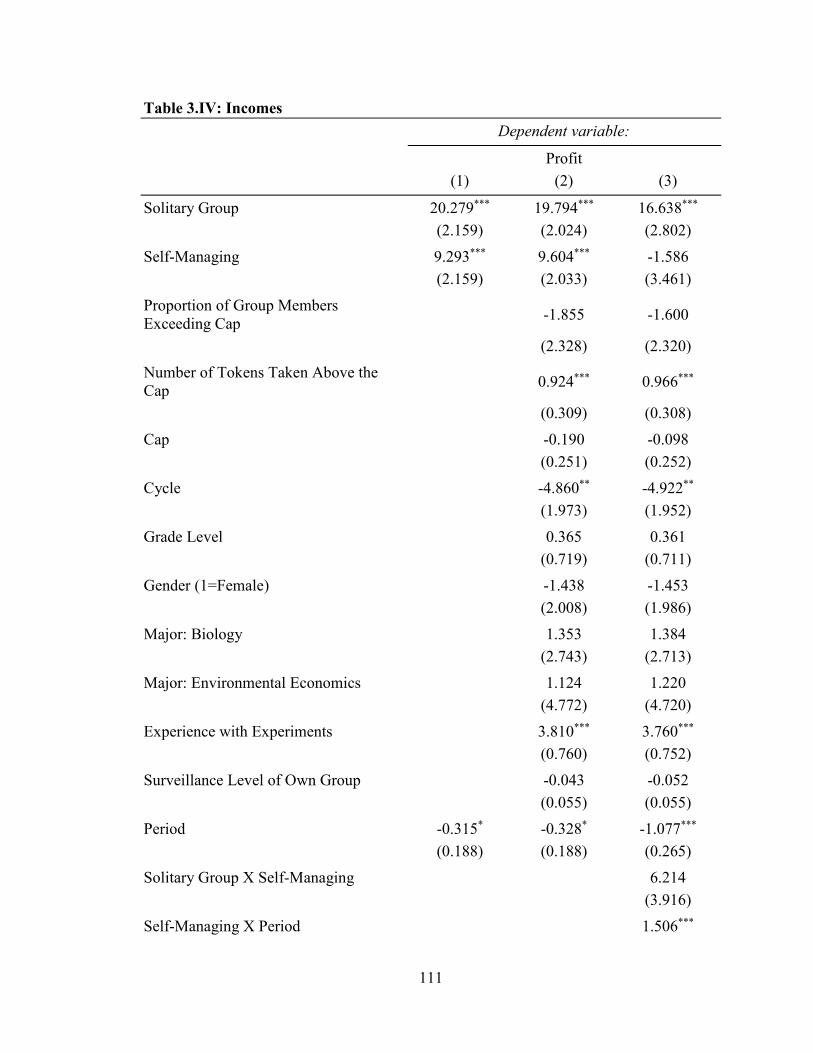
111
Table 3.IV: Incomes
Dependent variable:
Profit
(1) (2) (3)
Solitary Group 20.279*** 19.794*** 16.638***
(2.159) (2.024) (2.802)
Self-Managing 9.293*** 9.604*** -1.586
(2.159) (2.033) (3.461)
Proportion of Group Members Exceeding Cap
-1.855 -1.600
(2.328) (2.320)
Number of Tokens Taken Above the Cap
0.924*** 0.966***
(0.309) (0.308)
Cap
-0.190 -0.098
(0.251) (0.252)
Cycle
-4.860** -4.922**
(1.973) (1.952)
Grade Level
0.365 0.361
(0.719) (0.711)
Gender (1=Female)
-1.438 -1.453
(2.008) (1.986)
Major: Biology
1.353 1.384
(2.743) (2.713)
Major: Environmental Economics
1.124 1.220
(4.772) (4.720)
Experience with Experiments
3.810*** 3.760***
(0.760) (0.752)
Surveillance Level of Own Group
-0.043 -0.052
(0.055) (0.055)
Period -0.315* -0.328* -1.077***
(0.188) (0.188) (0.265)
Solitary Group X Self-Managing
6.214
(3.916)
Self-Managing X Period
1.506***
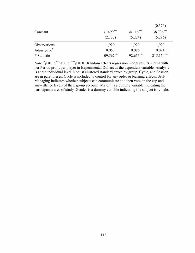
112
(0.376)
Constant 31.499*** 34.116*** 38.736***
(2.137) (5.224) (5.296)
Observations 1,920 1,920 1,920
Adjusted R2 0.053 0.086 0.094
F Statistic 109.562*** 192.656*** 215.154***
Note: *p<0.1; **p<0.05; ***p<0.01 Random effects regression model results shown with per Period profit per player in Experimental Dollars as the dependent variable. Analysis is at the individual level. Robust clustered standard errors by group, Cycle, and Session are in parentheses. Cycle is included to control for any order or learning effects. Self-Managing indicates whether subjects can communicate and then vote on the cap and surveillance levels of their group account. 'Major:' is a dummy variable indicating the participant's area of study. Gender is a dummy variable indicating if a subject is female.

113
Table 3.V: Harvesting
Dependent variable:
Own Group
Extraction
Own Group
Extraction
Own Group
Extraction Poaching Poaching
Total Extraction
Total Extraction
Total Extraction
(1) (2) (3) (4) (5) (6) (7) (8)
Solitary Group
2.677*** 0.704 1.052
-2.818*** -2.808*** -2.126***
(0.451) (0.775) (0.951)
(0.486) (0.500) (0.788)
Self-Managing
-2.112*** -1.944*** -0.300 0.387 0.439 -1.919*** -1.883*** -0.072
(0.451) (0.435) (0.717) (0.545) (0.628) (0.486) (0.496) (0.799)
Cap
0.047 0.040
-0.042
0.021 0.013
(0.040) (0.040)
(0.053)
(0.040) (0.040)
Cycle
0.520 0.521
0.483
0.598 0.601
(0.422) (0.416)
(0.579)
(0.482) (0.478)
Grade Level
0.150 0.150
0.049
0.161 0.160
(0.154) (0.152)
(0.211)
(0.176) (0.175)
Gender (1=Female)
-0.477 -0.475
0.109
-0.459 -0.454
(0.430) (0.424)
(0.601)
(0.492) (0.488)
Major: Biology
-0.139 -0.135
-0.505
-0.226 -0.228
(0.587) (0.580)
(0.982)
(0.672) (0.666)
Major: Environmental Economics
-0.326 -0.316
-1.202
-0.635 -0.639
(1.022) (1.008)
(1.168)
(1.168) (1.158)
Experience With Experiments
0.435*** 0.440***
-0.337*
0.351* 0.355*
(0.163) (0.160)
(0.204)
(0.185) (0.184)
Lagged Number of Tokens Poached by Other Group
0.036*** 0.036***
0.037***

114
(0.011) (0.011)
(0.014)
Lagged Surveillance of Other Group
-0.017 -0.016
0.003
0.002 0.003
(0.014) (0.014)
(0.019)
(0.015) (0.015)
Lagged Number of Tokens You Poached
0.051* 0.059**
(0.029) (0.029)
Tokens Poached
-0.774*** -0.771***
(0.027) (0.027)
Surveillance Level of Other Group
-0.026
-0.043*** -0.046***
(0.018)
(0.015) (0.015)
Surveillance Level of Own Group
0.006 0.006
0.051***
0.011 0.012
(0.009) (0.009)
(0.015)
(0.009) (0.009)
Period -0.024 -0.007 0.055 0.202*** 0.148** 0.077*** 0.013 0.099*
(0.035) (0.033) (0.057) (0.050) (0.059) (0.029) (0.033) (0.057)
Solitary Group X Self-Managing
-1.154
-1.475
(0.845)
(0.972)
Self-Managing X Period
-0.180***
-0.179***
(0.066)
(0.066)
Solitary Group X Period
0.053
0.007
(0.066)
(0.066)
Constant 12.501*** 12.548*** 11.861*** 4.190*** 2.517 17.344*** 16.341*** 15.568***
(0.435) (1.239) (1.265) (0.475) (1.588) (0.449) (1.182) (1.217)

115
Observations 1,920 1,728 1,728 960 864 1,920 1,728 1,728
Adjusted R2 0.028 0.346 0.349 0.015 0.030 0.027 0.032 0.036
F Statistic 57.555*** 929.540*** 942.911*** 16.649*** 40.122*** 56.382*** 69.332*** 80.093***
Note: *p<0.1; **p<0.05; ***p<0.01 Random effects regression model results shown. Analysis is at the individual level. Columns (1), (2), and (3) report regression results for token extraction from your own group account as the dependent variable. Columns (4) and (5) report regression results for token extraction from the other group's account as the dependent variable. Columns (4) and (5) restrict the sample to include only individuals in the connected group treatment, since only those individuals can poach. Columns (6), (7), and (8) report regression results for total token extraction from both your account and the other group's account (for connected groups) as the dependent variable. 'Lagged' indicates the value of the variable in the previous Period. Robust clustered standard errors by group, Cycle, and Session are in parentheses. Cycle is included to control for any order or learning effects. Self-Managing indicates whether subjects can communicate and then vote on the cap and surveillance levels of their group account. 'Major:' is a dummy variable indicating the participant's area of study. Gender is a dummy variable indicating if a subject is female.
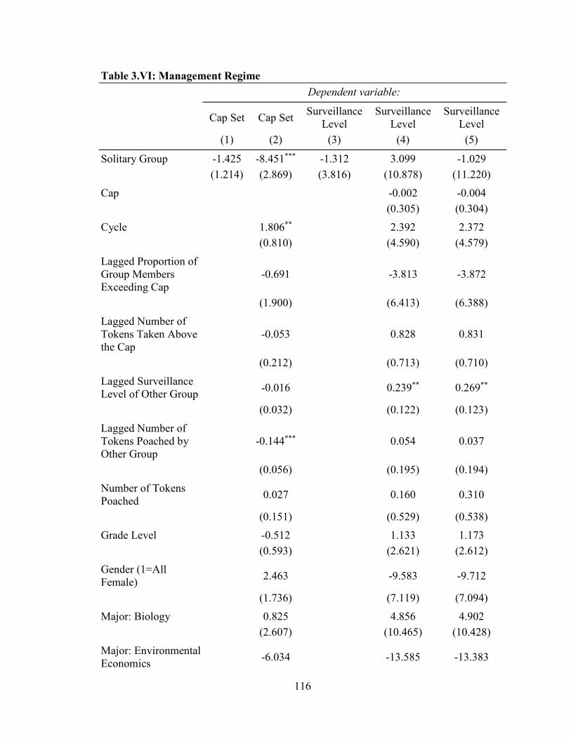
116
Table 3.VI: Management Regime
Dependent variable:
Cap Set Cap Set
Surveillance Level
Surveillance Level
Surveillance Level
(1) (2) (3) (4) (5)
Solitary Group -1.425 -8.451*** -1.312 3.099 -1.029
(1.214) (2.869) (3.816) (10.878) (11.220)
Cap
-0.002 -0.004
(0.305) (0.304)
Cycle
1.806**
2.392 2.372
(0.810)
(4.590) (4.579)
Lagged Proportion of Group Members Exceeding Cap
-0.691
-3.813 -3.872
(1.900)
(6.413) (6.388)
Lagged Number of Tokens Taken Above the Cap
-0.053
0.828 0.831
(0.212)
(0.713) (0.710)
Lagged Surveillance Level of Other Group
-0.016
0.239** 0.269**
(0.032)
(0.122) (0.123)
Lagged Number of Tokens Poached by Other Group
-0.144***
0.054 0.037
(0.056)
(0.195) (0.194)
Number of Tokens Poached
0.027
0.160 0.310
(0.151)
(0.529) (0.538)
Grade Level
-0.512
1.133 1.173
(0.593)
(2.621) (2.612)
Gender (1=All Female)
2.463
-9.583 -9.712
(1.736)
(7.119) (7.094)
Major: Biology
0.825
4.856 4.902
(2.607)
(10.465) (10.428)
Major: Environmental Economics
-6.034
-13.585 -13.383

117
(4.398)
(18.815) (18.751)
Experience with Experiments
2.382***
-1.808 -1.762
(0.803)
(3.500) (3.488)
Period -0.055 -0.066 0.421* 0.143 -0.262
(0.064) (0.081) (0.216) (0.272) (0.394)
Solitary Group X Period
0.755
(0.532)
Constant 12.221*** 14.119*** 16.684*** 10.890 12.563
(0.928) (3.389) (2.948) (14.126) (14.126)
Observations 160 144 160 144 144
Adjusted R2 0.001 0.164 0.012 -0.013 -0.005
F Statistic 2.112 40.965*** 3.916 12.202 14.301
Note: *p<0.1; **p<0.05; ***p<0.01 Random effects regression model results shown. Analysis is at the group level and restricted to self-managing groups. Columns (1) and (2) report regression results for the harvest cap the group selects as the dependent variable. Columns (3), (4), and (5) report regression results for the surveillance level the self-managing group selects as the dependent variable. 'Lagged' indicates the value of the variable in the previous Period. Robust clustered standard errors by group, Cycle and Session are in parentheses. Cycle is included to control for any order or learning effects. 'Major:' is a dummy variable indicating the proportion of group members majoring in that area of study.
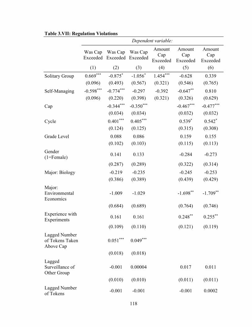
118
Table 3.VII: Regulation Violations
Dependent variable:
Was Cap Exceeded
Was Cap Exceeded
Was Cap Exceeded
Amount Cap
Exceeded
Amount Cap
Exceeded
Amount Cap
Exceeded
(1) (2) (3) (4) (5) (6)
Solitary Group 0.669*** -0.875* -1.056* 1.454*** -0.628 0.339
(0.096) (0.493) (0.567) (0.321) (0.546) (0.765)
Self-Managing -0.598*** -0.774*** -0.297 -0.392 -0.647** 0.810
(0.096) (0.220) (0.398) (0.321) (0.326) (0.629)
Cap
-0.344*** -0.350***
-0.467*** -0.477***
(0.034) (0.034)
(0.032) (0.032)
Cycle
0.401*** 0.405***
0.539* 0.542*
(0.124) (0.125)
(0.315) (0.308)
Grade Level
0.088 0.086
0.159 0.155
(0.102) (0.103)
(0.115) (0.113)
Gender (1=Female)
0.141 0.133
-0.284 -0.273
(0.287) (0.289)
(0.322) (0.314)
Major: Biology
-0.219 -0.235
-0.245 -0.253
(0.386) (0.389)
(0.439) (0.429)
Major: Environmental Economics
-1.009 -1.029
-1.698** -1.709**
(0.684) (0.689)
(0.764) (0.746)
Experience with Experiments
0.161 0.161
0.248** 0.255**
(0.109) (0.110)
(0.121) (0.119)
Lagged Number of Tokens Taken Above Cap
0.051*** 0.049***
(0.018) (0.018)
Lagged Surveillance of Other Group
-0.001 0.00004
0.017 0.011
(0.010) (0.010)
(0.011) (0.011)
Lagged Number of Tokens
-0.001 -0.001
-0.001 0.0002

119
Poached by Other Group
(0.007) (0.007)
(0.009) (0.009)
Number of Tokens Poached
-0.415*** -0.416***
-0.326*** -0.329***
(0.034) (0.034)
(0.022) (0.022)
Surveillance Level of Own Group
-0.011* -0.009
-0.021*** -0.021***
(0.006) (0.006)
(0.007) (0.007)
Period
0.0001 0.044 0.013 -0.004 0.050
(0.021) (0.044) (0.025) (0.027) (0.053)
Solitary Group X Self-Managing
-0.724*** -0.363
-1.225
(0.267) (0.515)
(0.885)
Solitary Group X Period
0.029
0.030
(0.057)
(0.074)
Self-Managing X Period
-0.097
-0.052
(0.066)
(0.075)
Solitary Group X Self-Managing X Period
-0.062
-0.170
(0.085)
(0.106)
Constant -0.506*** 4.210*** 4.060*** 1.982*** 8.398*** 7.632***
(0.082) (0.733) (0.758) (0.311) (0.920) (0.950)
Observations 1,920 1,919 1,919 1,920 1,728 1,728
Adjusted R2
0.010 0.210 0.219
Log Likelihood -1,239.873 -936.897 -931.523
F Statistic
22.282*** 472.729*** 501.110***
Note: *p<0.1; **p<0.05; ***p<0.01 Random effects regression model results shown for Columns (4), (5), and (6). Columns (1), (2), and (3) report logistic regressions. Analysis is at the individual level. Columns (1), (2), and (3) report logistic regression results for whether a subject exceeds the cap for the group account as the dependent variable. Columns (4), (5), and (6) report regression results for the amount that the group exceeds the cap as the dependent variable. Self-Managing indicates whether subjects can communicate and vote on the cap and surveillance levels of their group account. 'Lagged'

120
indicates the value of the variable in the previous Period. Robust clustered standard errors by group, Cycle, and Session are in parentheses. Cycle is included to control for any order or learning effects. 'Major:' is a dummy variable indicating the participant's area of study. Gender is a dummy variable indicating if a subject is female.

121
Figure 3.1: The relationship between group treatment and profit levels.

122
Figure 3.2: The relationship between management and profit levels.
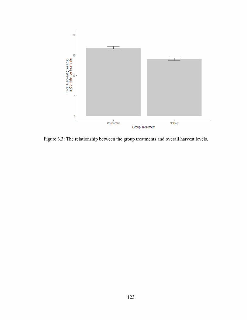
123
Figure 3.3: The relationship between the group treatments and overall harvest levels.

124
Figure 3.4: The relationship between management and overall harvest levels.

125
Figure 3.5: The relationship between the group treatment and the proportion of group
members who exceed the harvest cap.

126
APPENDICES
CHAPTER 2 APPENDIX Complete Original Ownership Analysis
If the measurement specification changes to encapsulate the entire round
(bargaining negotiation 1 between A and B, and negotiation 2 between C and the resulting
owner from negotiation 1), you find similar results as from just analyzing the first
negotiation’s outcome for all the variables except group size. There are no longer any
efficiency gains from adding a second taker. The specification from the main paper, just
analyzing efficiency from the first negotiation between A and B, is preferred because there
are two opportunities for a taker to take the token in the 3-person treatment but just one in
the 2-person treatment. More importantly, taker C does not face the recursive mechanism
of the Bar-Gill and Persico model because there is no taker to claim the token from them.
The absence of the mechanism means the absence of its efficiency inducing effects. To
compare efficiency impacts directly it is better to compare the results between just the first
negotiations. In the interest of completeness though, below are the results from an analysis
of retained ownership over the entire bargaining round.
Figure A2.1. The proportion of original owners of the token who
maintain possession of the token until the end of the entire round,
by group size. There is a noticeable difference in efficiency between
the 2-person treatment groups and the 3-person treatment groups
with the 3-person groups achieving statistically higher levels of
efficiency. 95 percent confidence intervals are shown.

127
Figure A2.2. The proportion of original owners of the token who
maintain possession of the token until the end of the entire
bargaining round, by information. The impact of incomplete
information on efficiency is statistically insignificant when analyzing
results by the entire bargaining round. 95 percent confidence
intervals are shown.
Incomplete information on how much the token is worth to your partner does not
have a significant impact when analyzing over the entire round. The results indicate
efficiency is 62.22 percent in the 2-person treatments and 75.29 percent in the 3-person
treatments; and 70.56 percent in the complete information and 66.67 percent in the
incomplete information treatments. Mann-Whitney-Wilcoxon tests confirm the rates of
ownership for original possessors are statistically significantly different from the theoretical
rate of 100 percent. Further Mann-Whitney-Wilcoxon tests confirm the impact of
complete information is not statistically significant and that the impact of adding a second
taker is statistically significant at the 1 percent level. The second taker brings a relative
increase in efficiency of 21.01 percent over the 2-person treatment scenario. To compare
to the analysis of just first negotiation outcomes, there the addition of a second taker
brought a relative increase of 38.09 percent.
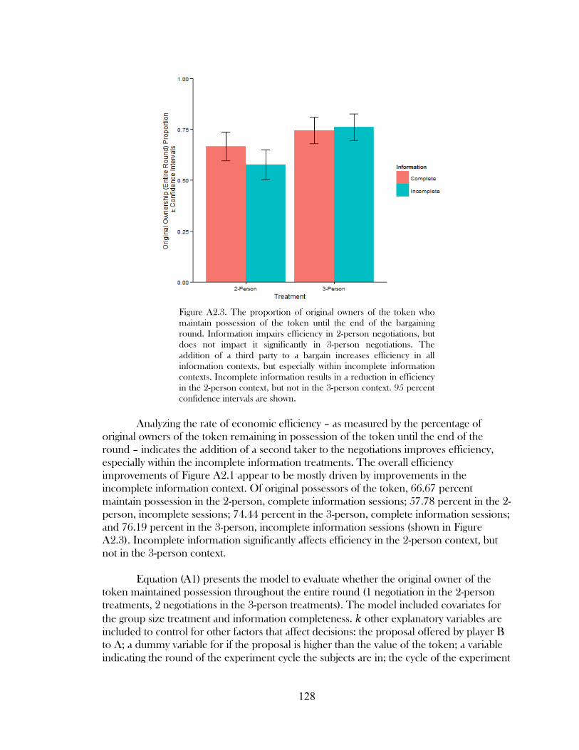
128
Figure A2.3. The proportion of original owners of the token who
maintain possession of the token until the end of the bargaining
round. Information impairs efficiency in 2-person negotiations, but
does not impact it significantly in 3-person negotiations. The
addition of a third party to a bargain increases efficiency in all
information contexts, but especially within incomplete information
contexts. Incomplete information results in a reduction in efficiency
in the 2-person context, but not in the 3-person context. 95 percent
confidence intervals are shown.
Analyzing the rate of economic efficiency – as measured by the percentage of
original owners of the token remaining in possession of the token until the end of the
round – indicates the addition of a second taker to the negotiations improves efficiency,
especially within the incomplete information treatments. The overall efficiency
improvements of Figure A2.1 appear to be mostly driven by improvements in the
incomplete information context. Of original possessors of the token, 66.67 percent
maintain possession in the 2-person, complete information sessions; 57.78 percent in the 2-
person, incomplete sessions; 74.44 percent in the 3-person, complete information sessions;
and 76.19 percent in the 3-person, incomplete information sessions (shown in Figure
A2.3). Incomplete information significantly affects efficiency in the 2-person context, but
not in the 3-person context.
Equation (A1) presents the model to evaluate whether the original owner of the
token maintained possession throughout the entire round (1 negotiation in the 2-person
treatments, 2 negotiations in the 3-person treatments). The model included covariates for
the group size treatment and information completeness. s other explanatory variables are
included to control for other factors that affect decisions: the proposal offered by player B
to A; a dummy variable for if the proposal is higher than the value of the token; a variable
indicating the round of the experiment cycle the subjects are in; the cycle of the experiment

129
session the negotiation is in; the number of economic experiments the subject had
participated in previously; and the negotiators’ gender and major.
"�t &(%) t *!"%*�),ℎ ���)= �� + �v)�0�� w� + �_x*S�)'!& �* + �y…aT��,y…a+ b�� (/1)
The results from a regression using Equation (A1) are reported in Table A2.1.
Column (1) reports the basic regression of ownership on the group-size and information
treatments. Column (2) reports a regression using Equation (A1), while Column (3) reports
a regression using Equation (A1) plus a control covariate indicating the player’s CRT score.
Column (3) only uses people who completed the CRT in less than 90 seconds.
Table A2.1: Ownership Analysis
Dependent variable:
Overall Ownership
(1) (2) (3)
3-Person Treatment 0.608*** 0.443* 0.153
(0.165) (0.238) (0.280)
Incomplete Information -0.172 -0.414* -0.551*
(0.163) (0.229) (0.305)
3-Person Treatment - 0.399 0.829*
X Incomplete Information (0.339) (0.450)
Proposal - -0.051*** -0.065***
(0.011) (0.014)
High Proposal - 1.127*** 1.320***
(0.346) (0.446)
Round - 0.301*** 0.378***
(0.103) (0.132)
Cycle - -0.144 -0.065
(0.173) (0.225)
Experience - -0.117** -0.107
(0.047) (0.141)
Gender (1=Female) - -0.071 -0.046
(0.173) (0.228)
Max Time to Comprehension - -0.000 -0.000
(0.001) (0.001)
UG Major: ENRE - -0.198 0.202

130
(0.300) (0.402)
UG Major: Biology - 0.050 -0.045
(0.213) (0.287)
Proportion CRT Correct - - -1.005
(0.952)
Constant 0.588*** 1.645*** 1.867***
(0.137) (0.448) (0.584)
Observations 708 708 441
AIC 871.38 844.11 527.37
Note: *p<0.1; **p<0.05; ***p<0.01 Logit regression. Clustered standard errors by the subject, cycle, and session are in parentheses. The unit of observation is at the subject level by session and cycle, and is considered repeated for all observations within a session and cycle. Column (1) gives the regression of whether the owner possesses the token after an entire round on the covariates of group size and information treatments. Column (2) reports the results of a regression based on Equation A1. Column (3) reports the preferred model of a regression (Equation A1) with a dummy variable for whether the original owner of the token maintains ownership of the token after the entire round as the dependent variable and controlling for CRT score. Participants who do not complete the CRT within 90 seconds are removed from the sample for the regression reported in Column (3).The 3-Person Treatment covariate is a dummy variable for if the subject is in the 3-subject sized group treatment. The Incomplete Information covariate is a dummy variable for if the subject is in the incomplete information treatment. Proposal indicates the bribe proposal offered by player B to A, and High Proposal is a dummy variable for if that proposal is higher than the value of the token to the original owner (30 Experimental Dollars). Experience, Gender, and UG Major control for demographic factors such as how many previous economic experiments the player has participated in, their gender, and their undergraduate major (Biology and Environmental and Natural Resource Economics are controlled for because of concerns the programs’ curricula would bias participants of those majors). Round and Cycle indicate the round of a cycle and the cycle of the session in which the proposal took place. Max Time to Comprehension indicates the longest time for a subject to correctly answer the comprehension questions between the owner of the token and the taker of the token. Proportion CRT Correct indicates the proportion of the 3 CRT questions the participant answered correctly.
Columns (1) and (2) of Table A2.1 indicate efficiency gains from the addition of a
second taker to the bargaining. However the coefficients on the addition are attenuated as
compared to those of Table 2.1 in the main paper. The output in Column (3) does not
have any statistically significant impact from the addition of a second taker. This contrasts
the results in Table 2.1. Besides the impacts from the treatments, the size of the proposal
offered (both the continuous variable and the High Proposal dummy variable) and the
round of the negotiation impact efficiency. Additionally the incomplete information and
the interaction between incomplete information and an additional taker are significant. The
proposal variables and round variable are also significant in Table 2.1. Since an analysis of
the entire round includes the second negotiation, where there is not another negotiation
afterwards with a taker for C to contend with, the mechanism of Bar-Gill and Persico is
significantly hampered. Therefore a reduction in the effect from adding a second taker is
not surprising. The effect disappears in Column (3) probably because the CRT model only
includes subjects who complete the test of decision-making skills within the time limit. This
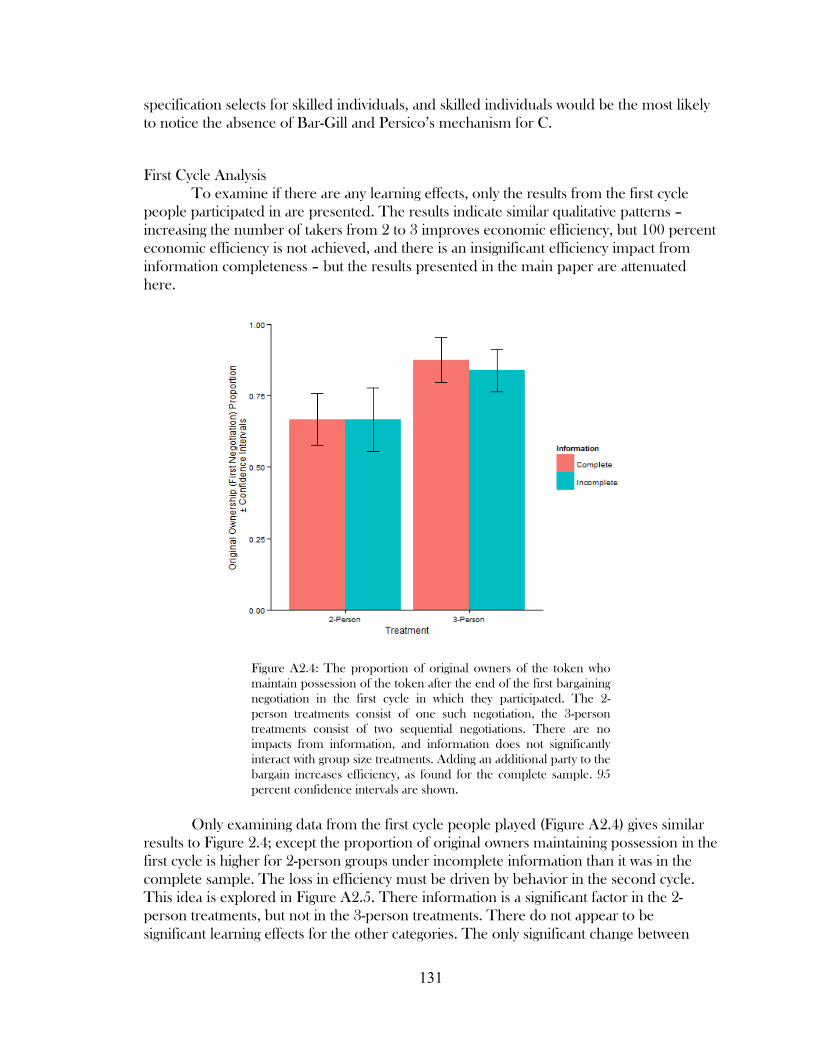
131
specification selects for skilled individuals, and skilled individuals would be the most likely
to notice the absence of Bar-Gill and Persico’s mechanism for C.
First Cycle Analysis
To examine if there are any learning effects, only the results from the first cycle
people participated in are presented. The results indicate similar qualitative patterns –
increasing the number of takers from 2 to 3 improves economic efficiency, but 100 percent
economic efficiency is not achieved, and there is an insignificant efficiency impact from
information completeness – but the results presented in the main paper are attenuated
here.
Figure A2.4: The proportion of original owners of the token who
maintain possession of the token after the end of the first bargaining
negotiation in the first cycle in which they participated. The 2-
person treatments consist of one such negotiation, the 3-person
treatments consist of two sequential negotiations. There are no
impacts from information, and information does not significantly
interact with group size treatments. Adding an additional party to the
bargain increases efficiency, as found for the complete sample. 95
percent confidence intervals are shown.
Only examining data from the first cycle people played (Figure A2.4) gives similar
results to Figure 2.4; except the proportion of original owners maintaining possession in the
first cycle is higher for 2-person groups under incomplete information than it was in the
complete sample. The loss in efficiency must be driven by behavior in the second cycle.
This idea is explored in Figure A2.5. There information is a significant factor in the 2-
person treatments, but not in the 3-person treatments. There do not appear to be
significant learning effects for the other categories. The only significant change between

132
Figure A2.4 and A2.5 is a reduction in efficiency in the 2-person treatments under
incomplete information in the second cycle comparing to the first cycle. Both Figure A2.4
and A2.5 show a significant improvement in efficiency with the addition of a second taker.
The efficiency improvement occurs in both information contexts.
Figure A2.5: The proportion of original owners of the token who
maintain possession of the token after the end of the first bargaining
negotiation in the second cycle in which they participated. The 2-
person treatments consist of one such negotiation, the 3-person
treatments consist of two sequential negotiations. 95 percent
confidence intervals are shown. Incomplete information reduces
efficiency in the 2-person groups, but has no significant effect in the
3-person groups. Adding an additional party improves efficiency in
all information contexts, but especially within the incomplete
information context.
Table A2.2: Proposal Analysis (Only Cycle 1)
Dependent variable:
Proposal
(1) (2)
3-Person Treatment 4.331 1.720
(4.193) (4.992)
Incomplete Information -2.317 -13.969**
(4.510) (6.540)
3-Person Treatment 2.343 16.321
X Incomplete Information (6.851) (9.886)
Proportion CRT Correct - -15.501
(15.215)

133
UG Major: Biology 7.76* -7.776*
(3.996) (3.996)
Observations 153 98
Adjusted R2 0.0.37 0.070
Note: *p<0.1; **p<0.05; ***p<0.01. Ordinary least squares regression. Clustered standard errors by the subject, cycle, and session are in parentheses. The unit of observation is at the subject level by session and cycle, and is considered repeated for all observations within a session and cycle. Reports a regression with the proposal made in the first negotiation as the dependent variable. The controls for (1) and (2) are the same as those reported in Table 2.3 Column (1) and Column (2). (2) includes all controls and CRT score while (1) does not include CRT score. We only report the coefficients on statistically significant variables from Table 2.3 here. Only observations from the first cycle of each session are reported, to identify learning effects.
Table A2.2 finds an impact from incomplete information in the first cycle. In the
first cycle first takers ask for significantly lower bribes than they do in cycle 2. Table A2.2
indicates learning effects occur for some populations in the experiment. The effect of CRT
score found in the model controlling for CRT (Table 2.3 Column (2)) is absent in the first
cycle. People who complete the CRT in time experience learning effects as the session
progresses and the significant coefficient of Table 2.3 is driven by their proposals in the
second cycle. In cycle 2 first takers offer significantly lower bribe proposals. The effect
from the biology program of study is similar. Interestingly in the first cycle subjects who do
not complete the CRT in time drive a sign change in the coefficient on biology from the
value Column (2) reports and the values Table 2.3 reports in Columns (1) and (2) to the
value shown in Column (1) of Table A2.2. The group size treatment effect is also absent in
both models.
Table A2.3: First Negotiation Ownership Analysis (Only Cycle 1)
Dependent variable:
Original Ownership (First Negotiation)
(1)
3-Person Group 1.380*** (0.522)
Incomplete Information -0.376
(0.529)
3-Person Group 0.384
X Incomplete Information (0.803)
Proposal -0.079***
(0.024)
High Proposal 1.978**
(0.769)
Round -0.081
(0.204)

134
Observations 351
AIC 230.7
Note: *p<0.1; **p<0.05; ***p<0.01 Logit regression. Clustered standard errors by the subject, cycle, and session are in parentheses. The unit of observation is at the subject level by session and cycle, and is considered repeated for all observations within a session and cycle. Column (1) reports the coefficients on the group-size treatment effect and on information incompleteness from the preferred model for a regression of whether the original owner of the token maintained ownership of the token after the first negotiation for only the first cycle. The controls are the same as those in Column (3) of Table 2.1. Column (1) controls for the CRT score and only people who completed the CRT within 90 seconds are included in the sample. A dummy variable indicating whether the original possessor of the token maintains ownership after the first negotiation is the dependent variable. The sample for Column (3) includes only observations from the first cycle of each experiment session.
Table A2.3 supports the finding that the addition of a second taker waiting to take
at the next negotiation improves economic efficiency in negotiations between an owner and
a first taker. The results are shown for the model that controls for CRT score. The results
for the complete sample are similar but are omitted for brevity. The coefficient on the 3-
person treatment dummy variable is comparable to that on the same variable in the model
which includes data from both cycles (1.436, also significant at the 1 percent level)....
High Proposal Analysis
A similar analysis to that reported in Table 2.3 looks at the offering of a proposal to
not take the token that is higher than the token is worth to the original owner. Regression
analysis does not identify any significant variables (Appendix Table A2.4). Descriptive
figures similar to those in the main paper are included (Appendix Figures A2.6-A2.8). The
results suggest incomplete information does not cause people to more frequently propose
more than the token is worth.
Table A2.4 shows the results for a model that controls for CRT score (Column 2)
and a model which does not (Column 1). A statistically significant impact from all
covariates except experience is absent in Column (2). The more experience you have with
economic experiments the more you propose bribes higher than the value of the token to
the owner.
Table A2.4: High Proposal Analysis
Dependent variable:
High Proposal
(1) (2)
3-Person Group 0.701* 0.160
(0.418) (0.498)
Incomplete Information 0.746** 0.530
(0.367) (0.452)
3-Person Group -0.423 -0.252
X Incomplete Information (0.532) (0.677)
Cycle -0.154 -0.238

135
(0.275) (0.615)
Gender (1=Female) 0.058 0.210
(0.286) (0.654)
Round 0.128 0.260
(0.166) (0.224)
Experience -0.071 0.434**
(0.083) (0.215)
UG Major: Biology -0.431 -0.468
(0.348) (0.468)
UG Major: ENRE 0.445 -0.429
(0.481) (0.661)
Comprehension 0.002** 0.002
(0.001) (0.002)
Constant -1.854*** 2.506***
(0.682) (0.919)
Observations 267 153
AIC 330.55 201.41
Note: *p<0.1; **p<0.05; ***p<0.01. Logit Regression. Clustered standard errors by the subject, cycle, and session are in parentheses. The unit of observation is at the subject level by session and cycle, and is considered repeated for all observations within a session and cycle. Observations are the proposals offered by taker B to owner A. Reports a regression with whether the proposal made in the first negotiation is higher than the value of the token to the owner as the dependent variable. The other controls are the same as those reported in Table 2.3 Columns (1) and (2). Comprehension indicates how long it took the subjects to complete the game comprehension questions at the beginning of the experiment. As in Table 2.3 Column (2) people who do not complete the CRT within 90 seconds are removed from the sample in Column (2).
Figures A2.6 and A2.7 show the treatment effects on whether subjects propose
more to not take the token than the token is worth. While Figure A2.7 indicates an effect
from information, the effect disappears once clustered standard errors by the subject, cycle,
and session are included. Figure A2.8 does not indicate any interaction effects between the
treatments and regression analysis confirms.

136
Figure A2.6. The proportion of proposals to not take the token that
are above the value of the token to the original owner, by group size.
Only results for the first negotiations are shown. The 3-person
group treatments have higher proportions of high proposals offered,
but the difference is only statistically significant at the 10 percent
level. 95 percent confidence intervals are shown.
Figure A2.7. The proportion of proposals to not take the token
above the value of the token to the original owner, by information.
The incomplete information treatments have statistically significant
higher proportions of high proposals being offered. 95 percent
confidence intervals are shown.

137
Figure A2.8: The proportion of proposals made to not take the token
that are greater than the value of the token, by group size and
information treatments. The Figure shows similar results to those
found in A2.6 and A2.7. There are not significant interaction effects
between information context and group size. 95 percent confidence
intervals are shown.
Proposal Behavior
Bribe proposals fall within the range predicted by the Bar-Gill and Persico model
and the experiment’s design, 0 < '^,� ≤ 30.
Proposal behavior is impacted by the completeness of information. Appendix
Figure A2.9, reports proposals of people under complete information and people under
incomplete information. The pattern of bribe proposals we expect to see is closely followed
in the complete information treatment. The expected pattern is smoothed under
incomplete information, intuitively because under incomplete information it is more
difficult for players to determine the efficient range.

138
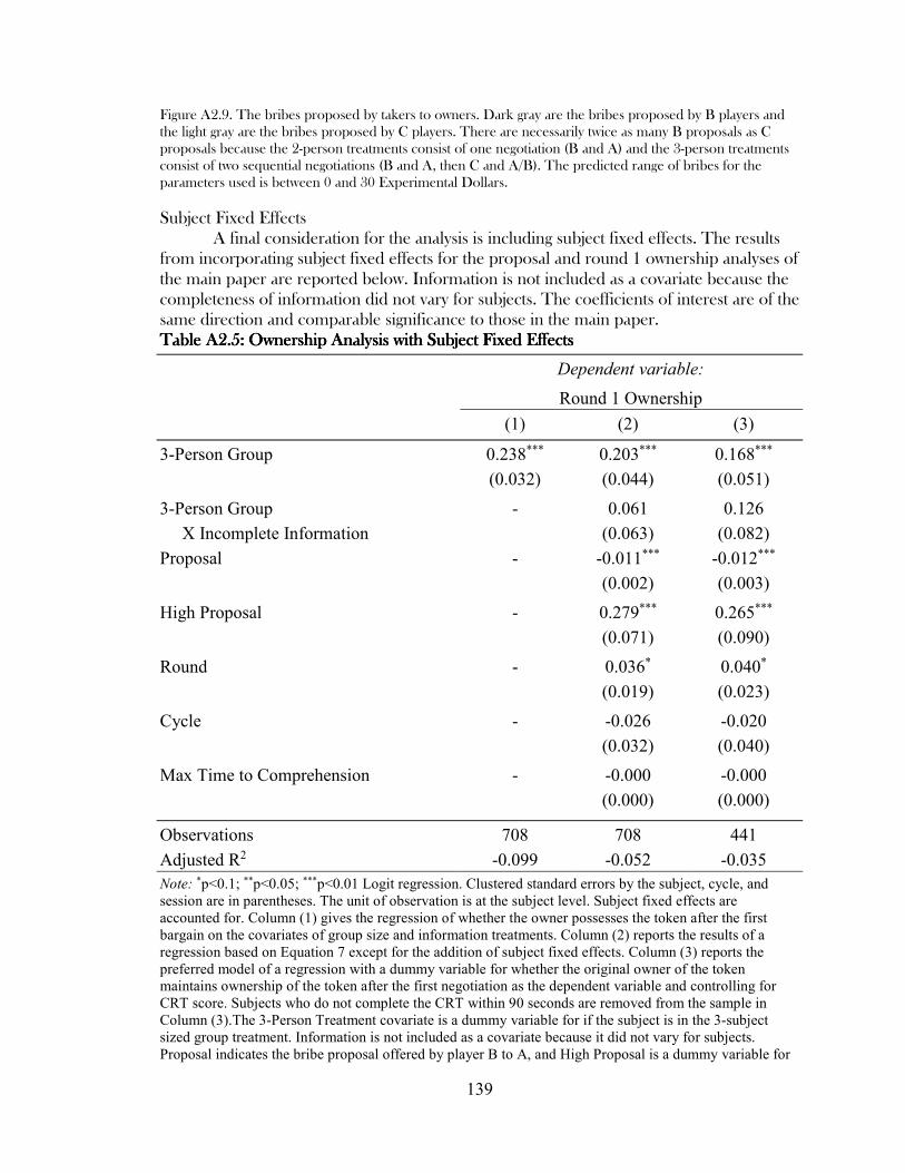
139
Figure A2.9. The bribes proposed by takers to owners. Dark gray are the bribes proposed by B players and
the light gray are the bribes proposed by C players. There are necessarily twice as many B proposals as C
proposals because the 2-person treatments consist of one negotiation (B and A) and the 3-person treatments
consist of two sequential negotiations (B and A, then C and A/B). The predicted range of bribes for the
parameters used is between 0 and 30 Experimental Dollars.
Subject Fixed Effects
A final consideration for the analysis is including subject fixed effects. The results
from incorporating subject fixed effects for the proposal and round 1 ownership analyses of
the main paper are reported below. Information is not included as a covariate because the
completeness of information did not vary for subjects. The coefficients of interest are of the
same direction and comparable significance to those in the main paper.
Table ATable ATable ATable A2.2.2.2.5: Ownership Analysis with Subject Fixed Effects5: Ownership Analysis with Subject Fixed Effects5: Ownership Analysis with Subject Fixed Effects5: Ownership Analysis with Subject Fixed Effects
Dependent variable:
Round 1 Ownership
(1) (2) (3)
3-Person Group 0.238*** 0.203*** 0.168***
(0.032) (0.044) (0.051)
3-Person Group - 0.061 0.126
X Incomplete Information (0.063) (0.082)
Proposal - -0.011*** -0.012***
(0.002) (0.003)
High Proposal - 0.279*** 0.265***
(0.071) (0.090)
Round - 0.036* 0.040*
(0.019) (0.023)
Cycle - -0.026 -0.020
(0.032) (0.040)
Max Time to Comprehension - -0.000 -0.000
(0.000) (0.000)
Observations 708 708 441
Adjusted R2 -0.099 -0.052 -0.035
Note: *p<0.1; **p<0.05; ***p<0.01 Logit regression. Clustered standard errors by the subject, cycle, and session are in parentheses. The unit of observation is at the subject level. Subject fixed effects are accounted for. Column (1) gives the regression of whether the owner possesses the token after the first bargain on the covariates of group size and information treatments. Column (2) reports the results of a regression based on Equation 7 except for the addition of subject fixed effects. Column (3) reports the preferred model of a regression with a dummy variable for whether the original owner of the token maintains ownership of the token after the first negotiation as the dependent variable and controlling for CRT score. Subjects who do not complete the CRT within 90 seconds are removed from the sample in Column (3).The 3-Person Treatment covariate is a dummy variable for if the subject is in the 3-subject sized group treatment. Information is not included as a covariate because it did not vary for subjects. Proposal indicates the bribe proposal offered by player B to A, and High Proposal is a dummy variable for

140
if that proposal is higher than the value of the token to the original owner. Round and Cycle indicate the round of a cycle and the cycle of the session in which the proposal took place. Max Time to Comprehension indicates the longest time for a subject to correctly answer the comprehension questions between the owner of the token and the taker of the token.
Table A2.5 reports similar qualitative findings to those of Table 2.1, but Table
A2.6 does not find group size to be a significant predictor of the size of bribe proposals
takers offer to owners. The same finding of the main paper.
Table ATable ATable ATable A2.2.2.2.6: Proposal Analysis with Subject Fixed Effects6: Proposal Analysis with Subject Fixed Effects6: Proposal Analysis with Subject Fixed Effects6: Proposal Analysis with Subject Fixed Effects
Dependent variable:
Proposal
(1) (2)
3-Person Group 2.839 0.139
(1.964) (2.234)
3-Person Group -1.512 2.261
X Incomplete Information (2.937) (3.764)
Round 0.658 0.719
(0.915) (1.130)
Cycle -0.008 -1.458
(0.009) (3.487)
Observations 267 153
Adjusted R2 -0.684 -0.739
Note: *p<0.1; **p<0.05; ***p<0.01. Ordinary least squares regression accounting for subject fixed effects. Clustered standard errors by the subject, cycle, and session are in parentheses. The unit of observation is at the subject. Reports a regression with the proposal made in the first negotiation as the dependent variable. The controls for (1) and (2) are the same as those reported in Table 2.3 Column (1) and Column (2) however only the treatment and time variables are included. The remaining variables either disappear with the addition of fixed effects (such as demographic variables) or are not shown because they were not significant in Table 2.3. (2) includes all controls and CRT score while (1) does not include CRT score.
Distribution Impacts
A further interesting aspect of the Bar-Gill and Persico model is the distribution of
wealth. With strong property rights, the original owners would receive 30 Experimental
Dollars, while takers receive nothing. In the experiment I find the average bribe paid to
takers is 20.29 Experimental Dollars. The benefits of the token are spread between the
takers and the owners. There is not a statistically significant impact from information
completeness, but the presence of a second taker does substantially reduce the money the
original owner receives at the end of the bargaining (Tables A2.7 and A2.8). The increased
efficiency we find is bought by the original owners of the token. The bribing by the owners
distributes wealth between takers and owners more evenly than would occur with strong
property rights.
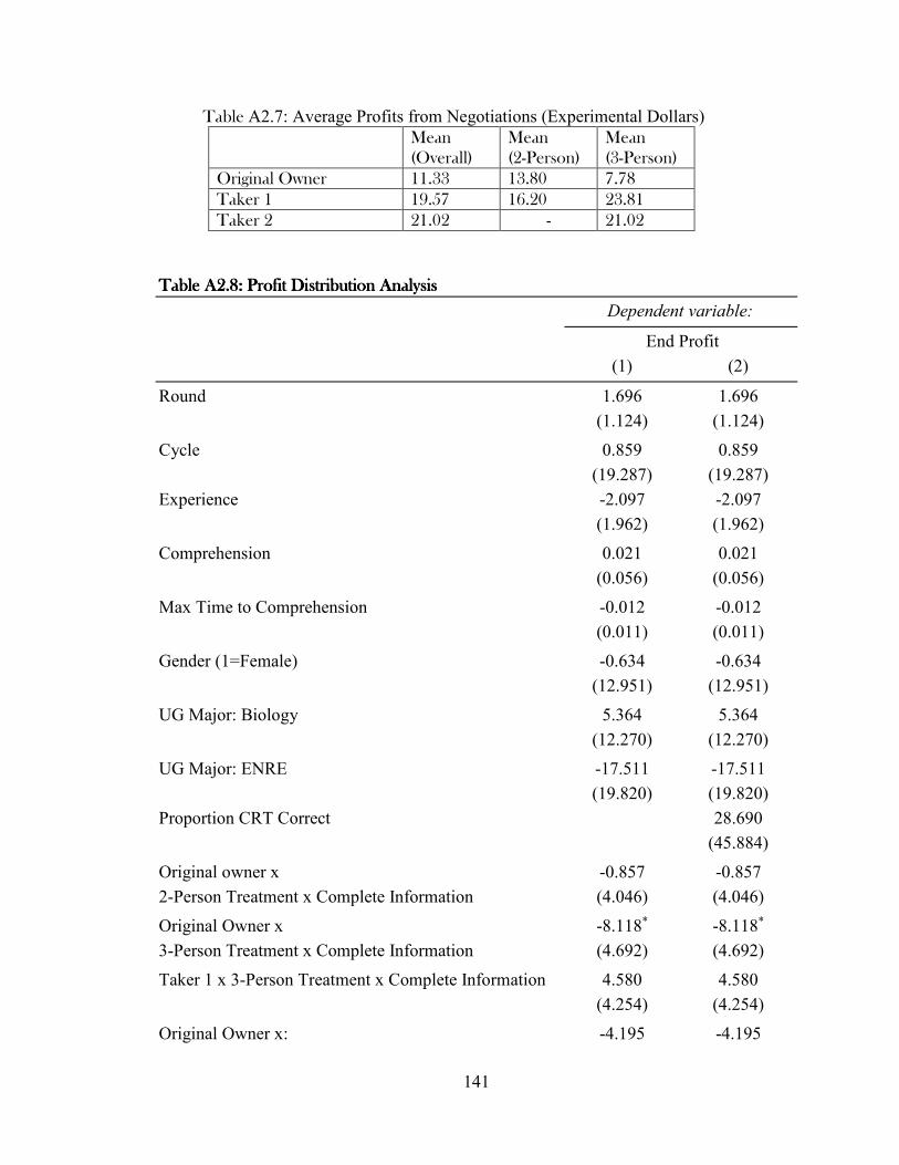
141
Table A2.7: Average Profits from Negotiations (Experimental Dollars)
Mean
(Overall)
Mean
(2-Person)
Mean
(3-Person)
Original Owner 11.33 13.80 7.78
Taker 1 19.57 16.20 23.81
Taker 2 21.02 - 21.02
Table ATable ATable ATable A2.2.2.2.8: Profit Distribution 8: Profit Distribution 8: Profit Distribution 8: Profit Distribution AnalysisAnalysisAnalysisAnalysis
Dependent variable:
End Profit
(1) (2)
Round 1.696 1.696
(1.124) (1.124)
Cycle 0.859 0.859
(19.287) (19.287)
Experience -2.097 -2.097
(1.962) (1.962)
Comprehension 0.021 0.021
(0.056) (0.056)
Max Time to Comprehension -0.012 -0.012
(0.011) (0.011)
Gender (1=Female) -0.634 -0.634
(12.951) (12.951)
UG Major: Biology 5.364 5.364
(12.270) (12.270)
UG Major: ENRE -17.511 -17.511
(19.820) (19.820)
Proportion CRT Correct
28.690
(45.884)
Original owner x -0.857 -0.857
2-Person Treatment x Complete Information (4.046) (4.046)
Original Owner x -8.118* -8.118*
3-Person Treatment x Complete Information (4.692) (4.692)
Taker 1 x 3-Person Treatment x Complete Information 4.580 4.580
(4.254) (4.254)
Original Owner x: -4.195 -4.195

142
2-Person Treatment x Incomplete Information (4.066) (4.066)
Original Owner x -18.147*** -18.147***
3-Person Treatment x Incomplete Information (3.980) (3.980)
Taker 1 x 3-Person Treatment x Incomplete Information 0.678 0.678
(3.986) (3.986)
Constant 5.224 5.224
(46.318) (46.318)
Observations 430 430
Adjusted R2 0.095 0.095
Note: *p<0.1; **p<0.05; ***p<0.01 Ordinary least squares regression. Clustered standard errors by the subject, cycle, and session are in parentheses. The unit of observation is at the subject level by session and cycle, and is considered repeated for all observations within a session and cycle. Reports a regression with the profit made by an individual at the end of the negotiation set as the dependent variable. Column (1) is a model including all subjects, while Column (2) reports results only using subjects who finished the CRT in time. 3-Person Treatment is a dummy variable for whether the subjects are in a cycle where they had 2 other members in their group. Incomplete Information is a dummy variable for whether the subjects are in a session where the available information is incomplete. Round and Cycle indicate the round of the cycle and the cycle of the session in which the proposal took place. Comprehension indicates how long it took the subjects to complete the game comprehension questions at the beginning of the experiment. UG major: indicates the participant’s area of study with “Other” as the base. Experience indicates how many previous economic experiments the subject had participated in previously. Proportion CRT Correct indicates the proportion of the 3 CRT questions the participant answered correctly.