three essays on the relation between trade and business
TRANSCRIPT
HAL Id: tel-02987297https://tel.archives-ouvertes.fr/tel-02987297
Submitted on 3 Nov 2020
HAL is a multi-disciplinary open accessarchive for the deposit and dissemination of sci-entific research documents, whether they are pub-lished or not. The documents may come fromteaching and research institutions in France orabroad, or from public or private research centers.
L’archive ouverte pluridisciplinaire HAL, estdestinée au dépôt et à la diffusion de documentsscientifiques de niveau recherche, publiés ou non,émanant des établissements d’enseignement et derecherche français ou étrangers, des laboratoirespublics ou privés.
Three essays on the relation between trade and businesscycle synchronization
Hoang-Sang Nguyen
To cite this version:Hoang-Sang Nguyen. Three essays on the relation between trade and business cycle synchronization.Economics and Finance. Université Rennes 1, 2019. English. �NNT : 2019REN1G014�. �tel-02987297�
THESE DE DOCTORAT DE
L'UNIVERSITE DE RENNES 1
COMUE UNIVERSITE BRETAGNE LOIRE
ÉCOLE DOCTORALE SCIENCES DE L’HOMME DES
ORGANISATIONSET DE LA SOCIETE (SHOS)
SCIENCES ECONOMIQUES ET SCIENCES DE GESTION
SPÉCIALITÉ: SCIENCES ÉCONOMIQUES
Par
Hoang-Sang NGUYEN
Three Essays on the Relation between Trade and
Business Cycle Synchronization
Thèse présentée et soutenue à Rennes, le 5 juillet 2019
Unité de recherche: CREM (UMR6211)
Rapporteurs avant soutenance:
Cécile Couharde Professeur, Université de Paris Nanterre Jean-Pierre Allegret Professeur, Université de Nice Sophia Antipolis
Composition du Jury:
Cécile Couharde Professeur, Université de Paris Nanterre / Rapporteur Jean-Pierre Allegret Professeur, Université de Nice Sophia Antipolis / Rapporteur Olivier Darné Professeur, Université de Nantes / Examinateur Vincent Vicard Economiste, CEPII / Examinateur Isabelle Cadoret-David Professeur, Université de Rennes 1 / Directrice de thèse Fabien Rondeau Maitre de conférences, Université de Rennes 1 / Co-directeur de thèse


This Ph.D. thesis should not be reported as representing the views of University of Rennes 1. The
views expressed are those of the author and do not necessarily reflect those of the University.
L’Université de Rennes 1 n’entend donner aucune approbation ni improbation aux opinons émises
dans cette thèse. Ces opinions doivent être considérées comme propres à leur auteur.

IV

v
Acknowledgements
It is my great pleasure to acknowledge and thank to those who helped along the way of
completing my research work. This thesis would not have been possible without their
guidance and help.
First and foremost, I would like to express my deep gratitude to my supervisors, Professor
Isabelle Cadoret-David and Doctor Fabien Rondeau. I thank them for giving me a chance
to come back to France, for their dedicated guidance, supervision, and very valuable
advices. I am deeply indebted to them for what they have done for me during last four years.
Without them, this thesis would not have been completed or written.
Besides my advisors, I would like to thank the rest of my thesis committee: Professor Cécile
Couharde from University Paris Nanterre, Professor Jean-Pierre Allegret from University
of Nice Sophia Antipolis, Professor Olivier Darné from University of Nantes and Doctor
Vincent Vicard from CEPII for their time, for their questions and comments.
I wish to express my sincere thanks to all members and staff of CREM and Faculty of
Economic Sciences, especially Madam Cécile Madoulet, Madam Anne L’Azou and
Madam Francoise Mazzoleni, for their helps and supports.
My sincere thanks also goes to all Ph.D. students in my laboratory. It was great sharing
office with all of you during last four years.
I am grateful to all my Vietnamese friends, who make my life in Rennes more interesting.
I owe my heartfelt thanks to my family, especially my parents and my wife Ngan Nguyen
for always encouraging and supporting me.
Lastly and most importantly, I thank my little daughter Clara Minh-Anh Nguyen - a small
navel of the universe that came and changed my life.
Hoang-Sang Nguyen

vi

vii
Résume en français
Trois essais sur la relation entre le commerce et la synchronisation des
cycles économiques
Depuis plusieurs décennies, la globalisation et l’intégration économique semblent
renforcer la convergence des cycles économiques des pays (Kose et al., 2008, Ductor and
Leiva-Leon, 2016). La synchronisation des cycles économiques constitue ainsi un sujet
important de la macroéconomie internationale. Plusieurs travaux de recherche ont testé
l’existence d’un cycle global unique (Otto et al., 2001, Stock et Watson, 2005, Kose et al.,
2008, Flood et Rose, 2010, Grigoraş et Stanciu, 2016, parmi d’autres). D’autres papiers ont
porté leur attention sur la mondialisation et l’européanisation des cycles économiques
(Crowley, 2008, Papageorgiou et al., 2010, Ferreira-Lopes et Pina, 2011, Pentecôte et
Huchet-Bourdon, 2012, Ahlborn et Wortmann, 2018, parmi d’autres). D’autres auteurs ont
évalué la transmission des cycles économiques en analysant la contagion des fluctuations
des variables macroéconomiques entre les pays et entre les régions (Sayek et Selover, 2002,
Osborn et al., 2005, Chen, 2009, Carstensen et Salzmann, 2017, Levchenko et Pandalai-
Nayar, 2018, Lange, 2018, parmi d’autres). L’identification des déterminantes de la
synchronisation des cycles est un défi essentiel en macroéconomie internationale. La
littérature met en évidence plusieurs facteurs : l’intégration commerciale, l’intégration
financière, la spécialisation industrielle, la coordination des politiques monétaires et
fiscales, les investissements directs à l’étranger, les régimes de change (Frankel et Rose,
1998, Clark et Van Wincoop, 2001, Fidrmuc, 2004, Imbs, 2004, Baxter et Kouparitsas,
2005, Inklaar et al., 2008, Abbott et al., 2008, Dées et Zorell, 2011, Pentecote et al., 2015,
parmi d’autres). Comme les volumes des échanges internationaux ont fortement augmenté
pendant les dernières années (de 17% du PIB mondial en 1960 à environ de 50% en 2017),
les effets du commerce bilatéral sur l’harmonisation des PIB ont attiré beaucoup d’attention
des chercheurs. Cette thèse vise ainsi à étudier empiriquement cet effet. Nous nous
concentrons sur trois questions qui ont reçu une attention limitée, voire nulle, dans la

viii
littérature existante : i) la propagation du choc de demande via le canal commerciale au sein
d'une zone monétaire et entre différentes zones monétaires, ii) le rôle de la marge extensive
du commerce dans la résolution du puzzle de commerce-synchronisation et iii) la
transmission des chocs de nouvelle de la productivité globale des facteurs (PGF) via le
commerce bilatéral. Les trois chapitres de cette thèse apportent des éléments de réponse à
ces questions.
Premièrement, la recherche se concentre sur la relation entre l’intégration
commerciale et les interdépendances macroéconomiques au sein de l’Union Européenne. Il
s’agit de mettre en évidence (i) le caractère endogène de l’intégration commerciale avec
l’élargissement de l’UE aux Pays de l’Europe Central et Orientale (PECO) et (ii) comment
cette intégration commerciale a eu des effets différents sur les interdépendances
macroéconomiques des PECO selon leur adoption ou non de l’euro. Pour répondre à ces
questions, nous utilisons dans le chapitre 1 un modèle quasi-VAR pour estimer des
changements dans les réponses de sept PECO1 aux chocs économiques qui viennent de
douze membres de la zone euro2 avant et après l’année 2004. Nos résultats empiriques
estimés sur la période 1990-2015 indiquent que les PECO sont affectés plus fortement par
les économies membres de la zone Euro pendant la période d’après 2004 qu’avant (3,3 fois
plus grande en moyenne). Les effets de contagion sont principalement expliqués par trois
économies les plus grandes de la zone euro qui sont l'Allemagne, la France et l'Italie. En
plus, les réponses des trois PECO qui ont rapidement adopté l'euro comme monnaie
nationale (Slovénie, Slovaquie et Estonie) sont plus élevées que celles des autres pays (4,9
contre 2,1) tandis que ses intensités commerciales avec la zone euro n’ont pas augmenté
(1,07 contre 1,12). L’adhésion à l'UE et l’adoption de l’euro permettent donc à ces pays
1 Sept PECO comprennent de République Tchèque, Estonie, Hongrie, Lituanie, Pologne, Slovaquie et
Slovénie. 2 Douze membres de la zone euro comprennent d’Autriche, Belgique, Finlande, France, Allemagne, Grèce,
Irlande, Luxembourg, Pays-Bas, Italie, Portugal et Espagne.

ix
d’amplifier les effets du commerce sur l’interdépendance macroéconomique et de s’intégrer
plus rapidement à la zone euro.
Le chapitre 2 va se concentrer sur les deux autres canaux par lesquels le commerce
augmente la synchronisation des cycles : la transmission de technologie et les effets des
termes de l’échange. Le principal apport du chapitre 2 est de distinguer les effets liés à la
marge extensive du commerce (nouveaux produits exportés) de la marge intensive du
commerce (produits déjà exportés). Kose et Yi (2006) a souligné le puzzle de commerce-
synchronisation selon lequel les modèles théoriques sont incapables de reproduire des effets
du commerce sur les corrélations du cycle économique aussi forts que ceux estimés par des
études empiriques. Comme Juvenal et Santos-Monteiro (2017), ce chapitre explique la
synchronisation des cycles économiques par trois facteurs: la corrélation de la PGF entre
deux pays, la corrélation de la part des dépenses en biens domestiques entre deux pays et
la corrélation entre la PGF d’un pays et la part des dépenses en biens domestiques de son
partenaire commercial. Ensuite, pour chaque facteur, les effets commerciaux sont
décomposés en deux parties : l’effet de la marge intensive et celui de la marge extensive.
En utilisant des données concernant 40 pays3 sur une période 1990-2015, nous trouvons
premièrement que la synchronisation des cycles économiques s'explique principalement par
la corrélation de la PGF et la corrélation de la part des dépenses en biens domestiques.
Deuxièmement, la marge extensive augmente non seulement la corrélation de la PGF entre
les partenaires commerciaux (Liao et Santacreu, 2015), mais aussi la corrélation entre les
parts de dépenses en biens domestiques. Le dernier effet est de 0.079 contre 0.074 qui sont
l’effet du commerce total (marge extensive et marge intensive) estimé par Juvenal et
Santos-Monteiro (2017). Ce résultat souligne que les nouveaux produits exportés
3 L’échantillon comprend de vingt-quatre pays développés (Australie, Autriche, Canada, Danemark,
Finlande, France, Allemagne, Grèce, Hongrie, Islande, Irlande, Italie, Japon, Corée du Sud, Pays-Bas,
Nouvelle-Zélande, Norvège, Pologne, Portugal, Espagne, États-Unis, Suède, Suisse et Royaume-Uni) et
seize pays émergents (Chili, Chine, Indonésie, Inde, Malaisie, Philippines, Argentine, Brésil, Mexique,
Turquie, Costa Rica, Roumanie, Thaïlande, Uruguay, Bulgarie et Tunisie).

x
transmettent les chocs de la PGF (la transmission de technologie) et ne détériorent pas,
voire améliorent, les termes de l'échange (les effets des termes de l’échange). Nous
suggérons donc qu’afin de résoudre le puzzle du commerce-synchronisation, il faut que les
modèles théoriques intègrent la marge extensive du commerce. Au niveau de politiques
économiques, pour augmenter la synchronisation des cycles, il faut que les pays créent un
environnement qui encourage les exports des nouveaux produits.
Troisièmement, le type de choc peut être une source du puzzle de commerce-
synchronisation. Dans les modèles DSGE, les fluctuations macroéconomiques sont souvent
générées à partir de chocs contemporains de la PGF. Néanmoins, plusieurs recherches
récentes ont démontré que les chocs de nouvelle de la PGF sont la source des cycles
économiques (Barsky et Sims, 2011, Beaudry et al., 2011b, Fujiwara et al., 2011, Nam et
Wang, 2015, Kamber et al., 2017, parmi d’autres). Le chapitre 3 étudie donc la transmission
des cycles économiques générée par ce type de chocs. Nous développons un modèle VAR
structurel et la méthodologie d’identification des chocs de nouvelles retenue est celle de
Barsky et Sims (2011 & 2017). La modélisation permet ainsi d’étudier les réponses de
l'Australie, du Canada, de la Nouvelle-Zélande et du Royaume-Uni aux chocs aux États-
Unis. Deux types de chocs sont évalués et comparés: i) un choc de nouvelles et ii) un choc
contemporain. L'exécution du modèle sur les données de la période post-Bretton Woods
(1973Q1-2016Q4) nous permet d’obtenir des résultats principaux. Premièrement, les chocs
de nouvelles de la PGF génèrent des cycles économiques aux États-Unis (le PIB et l’emploi
augmentent de 0,3% sur l’impact, l’investissement 1,5% et la consommation 0,2%) alors
que ce n’est pas le cas pour le choc contemporain. Deuxièmement, les effets des chocs de
nouvelles sur le taux de change réel, les termes de l'échange, les exportations et
importations bilatérales entre les petites économies ouvertes et les États-Unis sont différents
de ceux des chocs contemporains. Dans le cas d’un choc de nouvelles, les réponses du taux
de change réel et des termes de l'échange sont en forme de courbe en J. En revanche, elles
sont en forme de « U inversé » dans le cas d’un choc contemporain de la PGF. Face à un
choc favorable de la PTF aux États-Unis, les exportations des petits pays ouverts vers les
xi
États-Unis augmentent de façon permanente (les exportations du Canada et du Royaume-
Uni vers les États-Unis ont augmenté de 0,4% et de 0,3% sur l’impact, respectivement; les
exportations de l'Australie et de la Nouvelle-Zélande ont augmenté de 1,5% après le 5ème
trimestre et le 12ème trimestre, respectivement) alors que les importations enregistrent une
très légère augmentation dès le début et puis reviennent à zéro. Dans le cas d'un choc
contemporain de la PGF, les exportations augmentent puis reviennent rapidement à leur
niveau initial après quelques trimestres. Nous ne trouvons aucun effet de ce type de choc
sur les importations bilatérales. Troisièmement, les petites économies ouvertes sont
affectées par les cycles économiques aux États-Unis générées par les chocs de nouvelles.
Après l'augmentation des exportations vers Etats-Unis, le PIB, la consommation, l'emploi
et l'investissement des petits pays augmentent. En revanche, les réponses de ces économies
ne sont pas significatives dans le cas d'un choc contemporain de la PGF. Ainsi, le troisième
chapitre de cette thèse démontre que les chocs de nouvelle, en combinaison avec le
commerce bilatéral, peuvent être une source importante du cycle économique international.
Il faut que les économies augmentent les échanges avec les pays innovateurs (comme les
Etats-Unis) pour profiter les expansions économiques générées par les chocs de nouvelle
de la PGF.
La contribution principale de cette thèse est de fournir de preuves empiriques sur la
relation entre le commerce et la synchronisation des cycles. Les trois essais nous aident à
comprendre plus clairement comment le commerce bilatéral améliore la corrélation des
cycles économiques dans les cadres théoriques différents et pourquoi les modèles
théoriques ne parviennent pas à reproduire pleinement cette corrélation positive. Cette
compréhension est importante pour les implications politiques, notamment dans une zone
monétaire où les échanges commerciaux sont fortement encouragés, et le niveau élevé de
synchronisation des cycles économiques assure l’efficacité des politiques économiques
communes.

xii
References
Abbott, A., Easaw, J. and Tao Xing, 2008. Trade Integration and Business Cycle
Convergence: Is the Relation Robust across Time and Space? Scandinavian Journal of
Economics, Wiley Blackwell, vol. 110(2), pages 403-417, 06.
Ahlborn, M. and Wortmann, M., 2018. The core‒periphery pattern of European business
cycles: A fuzzy clustering approach. Journal of macroeconomics, Vol 55, Pages 12-27,
2018.
Barsky, Robert B. and Eric R. Sims. 2011. News shocks and business cycles. Journal of
Monetary Economics 58 (3): 273-289.
Baxter M. and Kouparitsas, M. A., 2005. Determinants of business cycle comove-ment: a
robust analysis. Journal of Monetary Economics, Elsevier, vol. 52(1), pages 113-157,
January.
Beaudry, P., Nam, D., Wang, J., 2011, Dec. Do mood swings drive business cycles and is
it rational? NBER Working Papers 17651. National Bureau of Economic Research, Inc.
Chen, Chien-Fu, 2009. Is the international transmission of business cycle fluctuation
asymmetric? Evidence from a regime-dependent ımpulse response function. Int. Res. J.
Finance Econ. 26, 134–143.
Clark T. E. and Van Wincoop, E., 2001. Borders and business cycles. Journal of
International Economics, Elsevier, vol. 55(1), pages 59-85, October.
Crowley, P.M., 2008. One money, several cycles? Evaluation of European business cycles
using model-based cluster analysis. Bank of Finland Research Discussion Papers 3/
2008. Bank of Finland, Helsinki.
Dées S. and Zorell N., 2012. Business Cycle Synchronisation: Disentangling Trade and
Financial Linkages. Open Economies Review, Springer, vol. 23(4), pages 623-643,
September.

xiii
Ductor, L., Leiva-Leon, D., 2016. Dynamics of global business cycle interdependence.
Journal of International Economics, Volume 102, 2016, Pages 110-127, ISSN 0022-
1996.
Ferreira-Lopes, A., Pina, A., 2011. Business cycles, core and periphery in monetary unions:
comparing Europe and North America. Open Econ. Rev. 22 (4), 565–592.
Fidrmuc, J., 2004. The endogeneity of the optimum currency area criteria, intra-industry
trade, and EMU enlargement. Contemporary Economic Policy 22, 1-12.
Flood, R. P., Rose, A.K., 2010. Inflation targeting and business cycle synchronization.
Journal of International Money and Finance, Volume 29, Issue 4, 2010, Pages 704-727,
ISSN 0261-5606.
Frankel, J. A. and Rose, A. K., 1998. The Endogeneity of the Optimum Currency Area
Criteria. Economic Journal, Royal Economic Society, vol. 108(449), pages 1009-25,
July.
Fujiwara, I., Hirose, Y., Shintani, M., 2011, 02. Can news be a major source of aggregate
fluctuations? A Bayesian DSGE approach. J. Money, Credit, Bank. 43 (1), 1–29.
Grigoraş, V., Stanciu, I. E., 2016. New evidence on the (de)synchronisation of business
cycles: Reshaping the European business cycle. International Economics, Volume 147,
2016, Pages 27-52, ISSN 2110-7017.
Imbs J., 2004. Trade, Finance, Specialization and Synchronization. The Review of
Economics and Statistics, MIT Press, vol. 86(3), pages 723-734, August.
Inklaar, R., Jong-A-Pin, R., de Haan, J., 2008. Trade and business cycle synchronization in
OECD countries — A re-examination. Eur. Econ. Rev. 52 (2), 646–666.
Juvenal, L., Santos Monteiro, P., 2017. Trade and synchronization in a multi-country
economy. European Economic Review, 97, 385-415.
Kamber G., Theodoridis K. and Thoenissen C., 2017. News-driven business cycles in small
open economies. Journal of International Economics 105 (2017): 77-89.
Kose, M.A., Otrok, C., Prasad, Eswar S., 2008. Global business cycles: convergence or
decoupling? IMF Working Paper WP/08/143.
xiv
Kose, M.A., Yi, K.-M., 2006. Can the standard international business cycle model explain
the relation between trade and comovement? Journal of International Economics. 68,
267– 295.
Lange, R.H., 2018. The effects of the U.S. business cycle on the Canadian economy: A
regime-switching VAR approach. The Journal of Economic Asymmetries, Volume 17,
2018, Pages 1-12, ISSN 1703-4949.
Levchenko and Pandalai-Nayar (forthcoming, Journal of the European Economic
Association). TFP, News, and "Sentiments. The International Transmission of Business
Cycles” (latest version Aug. 2018).
Liao W., and Santacreu A. M., 2015. The trade-comovement puzzle and the margins of
international trade. Journal of International Economics, Volume 96, Issue 2, Pages 266-
288, ISSN 0022-1996.
Nam, D. and Wang, J., 2015. The Effects of Surprise and Anticipated Technology Changes
on International Relative Prices and Trade. Journal of International Economics 97 (1):
162-177.
Papageorgiou, T., Michaelides, P.G., Milios, J.G., 2010. Business cycles synchronization
and clustering in Europe (1960–2009). Journal of Economics and Business, Volume 62,
Issue 5, 2010, Pages 419-470.
Pentecôte J.S., Huchet-Bourdon M., 2012. Revisiting the core-periphery view of EMU.
Economic Modelling, Volume 29, Issue 6, 2012, Pages 2382-2391, ISSN 0264-9993.
Pentecôte, J.S. Poutineau, JC. & Rondeau, F., 2015. Trade Integration and Business Cycle
Synchronization in the EMU: The Negative Effect of New Trade Flows. Open Econ.
Rev. (2015) 26: 61.
Otto, G., Voss, G., Willard, L., 2001. Understanding OECD output correlations. Research
Discussion Paper No. 2001/05.Reserve Bank of Australia.
Osborn, D.R., Perez, P.J., Sensier, M., 2005. Business cycle linkages for the G7 countries:
does the US lead the world? Centre for Growth and Business Cycle Research /
University of Manchester Discussion paper 050.

xv
Sayek, S., Selover, D.D., 2002. International interdependence and business cycle
transmission between Turkey and the European Union. South. Econ. J. 69 (2), 206–238.
Stock, J., Watson, M., 2005. Understanding changes in international business cycle
dynamics. J. Eur. Econ. Assoc. 50, 968–1006.

xvi

xvii
Contents
Acknowledgements.......................................................................................................... v
Résume en français ........................................................................................................ vii
Contents ...................................................................................................................... xvii
List of Figures .............................................................................................................. xix
List of Tables ................................................................................................................. xx
General Introduction ..................................................................................................... 1
Business Cycle Synchronization and Trade in a Globalizing World ............................... 1
References ................................................................................................................... 14
Chapter 1 The Transmission of Business Cycles: Lessons From the 2004 Enlargement
and the Euro Adoption ................................................................................................ 21
Highlights .................................................................................................................... 21
1.1. Introduction ....................................................................................................... 22
1.2. Literature Review .............................................................................................. 23
1.3. Model Specification and Data ............................................................................ 24
1.4. Empirical Results............................................................................................... 29
1.4.1. Effects of the 2004 Enlargement on Spillovers .............................................. 29
1.4.2. The Origins of the Spillovers ......................................................................... 36
1.4.3. Effects of the Euro on Spillovers ................................................................... 37
1.5. Conclusion......................................................................................................... 43
References ................................................................................................................... 46
Appendix ..................................................................................................................... 50
Chapter 2 Extensive Margin and Trade-Comovement Puzzle .................................. 54
Highlights .................................................................................................................... 54
2.1. Introduction and Literature Review.................................................................... 55
2.2. Methodology, Data and Measurement................................................................ 57
2.3. Empirical Results............................................................................................... 62
xviii
2.3.1 Stylized Facts .................................................................................................. 62
2.3.2 Business Cycle Comovement Factor Structure ................................................ 64
2.3.3 Margins of Trade and Business Cycle Comovement Factors ........................... 66
2.4. Robustness Checks ........................................................................................ 72
2.5. Conclusion ......................................................................................................... 77
References .................................................................................................................. 79
Appendix .................................................................................................................... 81
Chapter 3 News TFP Shock, Trade and Business Cycle Transmission to Small Open
Economies ..................................................................................................................... 83
Highlights ................................................................................................................... 83
3.1. Introduction and Literature Review ................................................................... 85
3.2. Empirical Strategy ............................................................................................ 89
3.2.1 SVAR Model and Estimation Strategy ............................................................ 89
3.2.2 News TFP Shock Identification Scheme ......................................................... 91
3.3. Data and Stylized Facts ..................................................................................... 94
3.4. Empirical Results .............................................................................................. 97
3.4.1. News TFP Shocks Generate Business Cycle in the United States ................... 97
3.4.2. Responses of Bilateral Trade and Relative Prices following Surprise and News
TFP Shocks ........................................................................................................... 100
3.4.3. Responses of Macro Aggregates of Small Open Countries following Surprise
and News TFP Shocks ........................................................................................... 106
3.4.4 . Forecast Error Variance Decomposition ...................................................... 114
3.5. Conclusion ...................................................................................................... 117
References ................................................................................................................ 119
General Conclusion .................................................................................................... 121
References ................................................................................................................ 125

xix
List of Figures
Figure 0.1 The United States’ business cycles, 1960–2018 .............................................. 2
Figure 0.2 Business cycles of the United States and the United Kingdom, 1960–2018 ..... 3
Figure 0.3 Trade intensity and business cycle synchronization for country pair groups,
from 1990–2015 ............................................................................................. 6
Figure 1.1 Change in multiplier effect and change in trade intensity .............................. 33
Figure 1.2 Responses of CEECs to common shocks....................................................... 35
Figure 2.1 Extensive and intensive margins of trade ...................................................... 63
Figure 3.1 US utilization-adjusted Total Factor Productivity (1973Q1–2017Q3) ........... 95
Figure 3.2 Impulse responses of US macro aggregates to a surprise TFP shock ............. 98
Figure 3.3 Impulse responses of US macro aggregates to a news TFP shock ............... 100
Figure 3.4 Impulse responses of trade and relative price variables in small open
economies to a surprise TFP shock in the United States .................................... 102
Figure 3.5 Impulse responses of trade and relative price variables in small open
economies to a news TFP shock in the United States ......................................... 104
Figure 3.6 Impulse responses of trade and relative price variables in small open
economies to a news TFP shock in the United States ......................................... 108
Figure 3.7 Impulse responses of macro aggregates in small open economies to a news
TFP shock in the United States ................................................................................ 111

xx
List of Tables
Table 1.1 Multiplier effects and trade intensity after/before 2004 ................................... 31
Table 1.2 Degree of shock diffusion and ranking ........................................................... 37
Table 1.3 Effect of adopting the euro ............................................................................. 39
Table 1.4 Mean of ratios of multiplier effects and trade intensity (CEECs’ responses for a
shock in EA-12) ............................................................................................. 39
Table 1.5 Panel Estimations for moving-window coefficients MM24
(2004:02 - 2015:02) ....................................................................................... 42
Table 1.A.1 Model specification tests ............................................................................. 50
Table 1.A.2 Chow tests (P-values) for breaks in near-VAR models ................................ 51
Table 1.A.3 Residual analysis ........................................................................................ 52
Table 1.A.4 Multiplier effects before and after the accession (in percent)....................... 53
Table 2.1 Business cycle synchronization factor structure .............................................. 65
Table 2.2 Output comovement and bilateral trade – a revisit .......................................... 67
Table 2.3 Bilateral trade and TFP comovement .............................................................. 69
Table 2.4 Bilateral trade and share of expenditure on domestic goods comovement ....... 70
Table 2.5 Bilateral trade and the correlation between TFP and expenditure share on
domestic goods .............................................................................................. 71
Table 2.6 Correlations and margins of trade using series of growth ................................ 72
Table 2.7 Correlations and margins of trade using GMM-IV .......................................... 73
Table 2.8 Correlations and margins of trade, 1990–2006 ................................................ 73
Table 2.9 Correlations and margins of trade in capital goods .......................................... 74
Table 2.10 Correlations and margins of trade in consumption goods .............................. 75
Table 2.11 Correlations and margins of trade in intermediate goods ............................... 75

xxi
Table 2.12 Correlations and margins of trade in intermediate goods with dummy
instrument variable ........................................................................................ 76
Table 2.13 Extensive and intensive margin measured only using exports ....................... 76
Table 2.A.1 Descriptive Statistics .................................................................................. 81
Table 2.A.2 Our results versus Liao and Santacreu (2015) and Juvenal and Santos-
Monteiro (2017)............................................................................................. 82
Table 3.1 Relative GDP size and Trade Intensity between four countries and the United
States (1973–2016) ........................................................................................ 96
Table 3.2 Summary of results ...................................................................................... 113
Table 3.3 Surprise TFP shock: variance decomposition ............................................... 115
Table 3.4 News TFP shock: variance decomposition ................................................... 116

xxii
1
GENERAL INTRODUCTION
BUSINESS CYCLE SYNCHRONIZATION AND TRADE IN A
GLOBALIZING WORLD
In a globalizing world with rapidly increasing trade and financial integration, economies
becoming more integrated. While emerging countries could benefit from the economic
growth of industrial countries, they could also suffer from the collapses in these economies.
A small open economy such as Canada may fluctuate together with its giant neighbor, the
United States. A productivity shock in the euro area may influence the employment rate in
Central and Eastern European countries (CEECs). Moreover, when China sneezes, others
Asian economies catch a cold. The first decade of this century has seen the Great Recession,
which affected most countries around the world. The world is increasingly “flat,” and many
countries’ business cycles are converging (Kose et al., 2008, Ductor and Leiva-Leon, 2016).
In macroeconomics, the business cycle of an economy is defined as the rises and
falls in gross domestic product (GDP) around its long-term trend. More specifically, it
describes the series of expansion and contraction periods. These fluctuations originate from
uncertainty shocks: policy shock, productivity shock, customer confidence shock, and other
demand and supply shocks. Business cycles are usually measured as the cyclical
components of real output. Figure 0.1 depicts the United States’ business cycles and its
long-term trend between 1960–2018. The figure clearly indicates the recession periods of
the United States’ economy over last decades: 1969–1970, 1973–1975, 1980–1982, 1990–
1991, 2001–2002 and 2007–2009. These periods are identified as recession time by the
Business Cycle Dating Committee (NBER). The business cycles synchronization (business
cycle comovement) describes the harmonization of real activity fluctuations across
countries resulting from the economic integration. In the literature, it is usually measured
as the correlation coefficient between cyclical components of the real GDP of economies.

2
For example, business cycle comovement is illustrated in Figure 0.2, which depicts business
cycles of the United States and United Kingdom from 1960–2018. The figure highlights
that the United Kingdom’s economy went down when the United States’ economy
experienced recessions. In fact, the output correlation coefficient between these two
economies is approximately 0.70 over the considered period.
Figure 0.1 The United States’ business cycles, 1960–2018
Notes: Source: Author’s calculation based on data extracted from the OECD database. The Hodrick-Prescott (HP) filter is used to detrend the GDP series. Unit: thousands of trillion US 2010 dollars. Axis: The United
States real GDP and HP trend correspond to left axis; the United States business cycles corresponds to the
right axis.
-0.5
-0.4
-0.3
-0.2
-0.1
0.0
0.1
0.2
0.3
0.4
2
4
6
8
10
12
14
16
18
Q1-
1960
Q4-
1961
Q3-
1963
Q2-
1965
Q1-
1967
Q4-
1968
Q3-
1970
Q2-
1972
Q1-
1974
Q4-
1975
Q3-
1977
Q2-
1979
Q1-
1981
Q4-
1982
Q3-
1984
Q2-
1986
Q1-
1988
Q4-
1989
Q3-
1991
Q2-
1993
Q1-
1995
Q4-
1996
Q3-
1998
Q2-
2000
Q1-
2002
Q4-
2003
Q3-
2005
Q2-
2007
Q1-
2009
Q4-
2010
Q3-
2012
Q2-
2014
Q1-
2016
Q4-
2017
US real GDP HP Trend Cycle

3
Figure 0.2 Business cycles of the United States and the United Kingdom, 1960–2018
Notes: Source: Author’s calculation based on data extracted from OECD database. The HP filter is used to
detrend the GDP series. Unit: thousands of trillion US 2010 dollars. Axis: the United States business cycles
correspond to left axis; the United Kingdom business cycles corresponds to right axis.
Business cycle synchronization is an important contemporary subject in
international macroeconomics. It has attracted interest from researchers because of its
policy implications. For example, when member countries in a common currency area
exhibit high levels of GDP comovement, common economic policies have more symmetric
impacts and therefore, more success (Mundell, 1961). By understanding the business cycle
comovement, one may forecast the extent to which a shock in one country propagates to
others. Thus, theorists focus on explaining business cycle comovement. Empirical research
has sought evidence on business cycle convergence. For instance, authors such as Otto et
al. (2001), Stock and Watson (2005), Kose et al., (2008), Flood and Rose (2010), and
Grigoraş and Stanciu (2016), among others, have studied the existence of a global business
cycle. An international business cycle requires the convergence of macro fluctuations
across countries. In other words, output and other macroeconomic aggregates across
-0.04
-0.03
-0.02
-0.01
0.00
0.01
0.02
0.03
0.04
0.05
-0.50
-0.40
-0.30
-0.20
-0.10
0.00
0.10
0.20
0.30
0.40Q
1-19
60
Q4-
1961
Q3-
1963
Q2-
1965
Q1-
1967
Q4-
1968
Q3-
1970
Q2-
1972
Q1-
1974
Q4-
1975
Q3-
1977
Q2-
1979
Q1-
1981
Q4-
1982
Q3-
1984
Q2-
1986
Q1-
1988
Q4-
1989
Q3-
1991
Q2-
1993
Q1-
1995
Q4-
1996
Q3-
1998
Q2-
2000
Q1-
2002
Q4-
2003
Q3-
2005
Q2-
2007
Q1-
2009
Q4-
2010
Q3-
2012
Q2-
2014
Q1-
2016
Q4-
2017
US Business Cycles UK Business Cycles
4
countries move in the same rhythm. There is evidence that national fluctuations around the
world are increasingly correlated, and therefore, an international business cycle may exist
(Kose et al. 2008, Ductor and Leiva-Leon, 2016). However, there is also evidence that
suggests a decrease in the correlation of cycle components of outputs, or the single business
cycle, does not exist (Camacho et al., 2006, Grigoraş and Stanciu, 2016). The existence of
a global business cycle is still being debated, although to some extent, economies are
moving together.
Several papers have focused on the globalization or, notably, the Europeanization
of the business cycle. These studies have exploited a core-periphery framework to evaluate
the convergence of business cycle of peripheries toward core economies. This strand of
research includes the works of Crowley (2008), Papageorgiou et al. (2010), Ferreira-Lopes
and Pina (2011), Pentecôte and Huchet-Bourdon (2012), and Ahlborn and Wortmann
(2018), among others. There is evidence that members of regions around the world
experience core-periphery patterns wherein the periphery business cycle converges to the
systematic core. However, the definition of “core” remains debated. For example, most
studies have used Germany as the proxy for business cycles of the euro area. Other studies
have assumed that the main members of this region exhibit a unified business cycle and
that the macro aggregates of periphery countries converge accordingly. However, there is
limited empirical verification of this assumption.
Another line of research, including studies conducted by Sayek and Selover (2002),
Osborn et al. (2005), Chen (2009), Carstensen and Salzmann (2017), Levchenko and
Pandalai-Nayar (2018), and Lange (2018), among others, has evaluated the transmission of
business cycles by investigating spillovers from a specific country or region to another. In
these cases, there is evidence that the transmission of business cycle from one economy to
others is significant. For instance, Lange (2018) has illustrated that 55% to 70% of a shock
to the United States’ output gap is transmitted to Canada within the first year after the shock.
Using a larger sample, Carstensen and Salzmann (2017) have indicated that 10% to 25%
5
variance of the G7 countries’ output growth is effected by the non-G7-countries’ business
cycle.
Thus, the transmission and convergence of the business cycles of economies has
been well documented in the literature. As such, an important question is, what forces the
real output comovement? Frankel and Rose (1998), Clark and Van Wincoop (2001),
Fidrmuc (2004), Imbs (2004), Baxter and Kouparitsas (2005), Inklaar et al., (2008), Abbott
et al. (2008), Dées and Zorell (2012), and Pentecôte et al. (2015), among others, have
addressed this problem. These studies have documented that trade integration is one of the
most important determinants of business cycle comovement. Moreover, financial
integration, industrial specialization, international coordination of monetary and fiscal
policy, (horizontal and vertical) foreign direct investment, firm-level linkages, and
exchange rate regimes, etc., are also sources of macro aggregates’ comovement across
countries.
This dissertation focuses on the impacts of bilateral trade on business cycle
synchronization. According to World Bank data, world total trade has increased from 17%
in 1960 to approximately half of the world GDP in 2017. With this impressive increase
over recent decades, the role of trade with respect to economic integration between
countries is incontrovertible. Figure 0.3 visualizes the trade-comovement relationship. In
fact, the figure summarizes 780 observations from a sample of twenty-four developed
countries and sixteen developing countries between 1990 and 2015 4 . As the figure
4 Data is extracted from OECD, IMF and World Bank databases and concerns 40 countries, including
twenty-four developed countries (Australia, Austria, Canada, Denmark, Finland, France, Germany, Greece,
Hungary, Iceland, Ireland, Italy, Japan, South Korea, the Netherlands, New Zealand, Norway, Poland,
Portugal, Spain, Sweden, Switzerland, the United Kingdom and the United States) and sixteen developing countries (Chile, China, Indonesia, India, Malaysia, Philippines, Argentina, Brazil, Mexico, Turkey, Costa
Rica, Romania, Thailand, Uruguay, Bulgaria and Tunisia). Output comovement is measured as the first-
differenced correlation of real GDP between two countries. Trade intensity in logarithm is calculated as follows:
)()()(i
ji
j
ij
ijTotalIM
IMLog
TotalIM
IMLogsityTradeIntenLog where IMij denotes import from i to j, IMji
is import from j to i, TotalIMi and TotalIMj are total import of country i and country j, respectively.
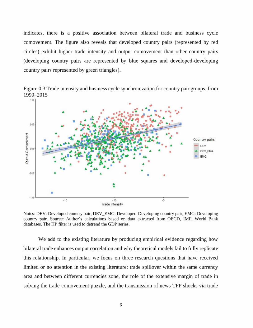
6
indicates, there is a positive association between bilateral trade and business cycle
comovement. The figure also reveals that developed country pairs (represented by red
circles) exhibit higher trade intensity and output comovement than other country pairs
(developing country pairs are represented by blue squares and developed-developing
country pairs represented by green triangles).
Figure 0.3 Trade intensity and business cycle synchronization for country pair groups, from
1990–2015
Notes: DEV: Developed country pair, DEV_EMG: Developed-Developing country pair, EMG: Developing
country pair. Source: Author’s calculations based on data extracted from OECD, IMF, World Bank
databases. The HP filter is used to detrend the GDP series.
We add to the existing literature by producing empirical evidence regarding how
bilateral trade enhances output correlation and why theoretical models fail to fully replicate
this relationship. In particular, we focus on three research questions that have received
limited or no attention in the existing literature: trade spillover within the same currency
area and between different currencies zone, the role of the extensive margin of trade in
solving the trade-comovement puzzle, and the transmission of news TFP shocks via trade

7
channels. The first and the last questions relate to the demand-supply spillover channel of
trade. The second question addresses the technology transmission channel of trade and the
terms-of-trade effect. Therefore, this dissertation studies three mechanisms through which
bilateral trade enhances the business cycle synchronization, as documented in the existing
literature (Liao and Santacreu, 2015).
The chapters of this dissertation address the aforementioned questions. First,
Chapter 1 focuses on the effects of trade on contagion in the European Union. Twenty years
have passed since the creation of the euro area on January 1, 1999. During this time, seven
potential candidates have adopted the euro (Greece, 2001, Slovenia, 2007, Cyrus, 2008,
Malta, 2008, Estonia, 2011, Latvia, 2014, Lithuania, 2015). It is interesting to study trade
spillover effects in a common currency area, especially for new members. It is also
interesting to review the endogeneity of the Optimum Currency Areas documented by
Frankel and Rose (1998), who have suggested that a common currency increases trade ex-
post and so, the synchronization of business cycle between members. However, the
differences in effects of trade within the same currency area and between different currency
zones should also be addressed. As such, Chapter 1 sheds some light on these problems by
investigating the trade spillover effects and business cycle interdependences in the
European Union. In particular, we estimate the trade spillover effects of twelve founding
members of the euro area on seven CEECs. By running a near-VAR model that captures
direct and indirect effects of trade between 1996 and 2015, we determine three main results:
the primary economies of the euro area (Germany, France and Italy) diffuse spillover effects
on CEECs; CEECs respond more strongly to output shocks in the euro area after becoming
members of the European Union in 2004; and, most importantly, the adoption of the euro
significantly enhances macro interdependences but without higher trade intensity. Trade
intensity increases business cycle synchronization within the same currency area, but the
effects are negative for CEECs without the euro. These results reveal that a common
currency amplifies trade effects for business cycle interdependences but does not increase
trade intensity, especially for periphery members of the common currency area.

8
Chapter 1 adds to the literature by producing empirical evidence regarding the
demand-supply spillover channel through which trade enhances output comovement. The
demand-supply spillover channel presented in the standard model (Backus et al., 1995)
indicates that economies with higher trade intensity are more synchronized because trade
increases the demand for foreign (intermediate) goods. More specifically, a positive
demand (supply) shock induces an increase in domestic GDP and its demand for import.
Therefore, foreign GDP also increases after the shock due to the increase in its export.
Hence, the real activity fluctuations in an open economy are transmitted to trading partners.
To demonstrate this relationship, Ng (2010) has presented a simple example: suppose that
country X exports intermediate goods to country Y. In Country Y, these imported
intermediate goods are combined with domestic intermediate goods in processes of
production of final goods, which are consumed domestically or exported to country X or a
third country, Z. Intermediate goods from country X are complements to country Y’s
intermediate and final goods. A demand shock occurring in country X, Y or Z requires an
increase in final good production, thereby increasing demand for intermediate goods from
countries X and Y. The real outputs of countries X and Y will thus increase together and
co-move. If country Y experiences a supply shock, the demand for country X’s intermediate
goods will increase because these goods are also necessary for final goods production. In
this case, the real outputs of countries X and Y also increase together. As a result, the
demand-supply spillover is a mechanism through which trade positively influences real
activity comovement. However, the existing literature has also documented other
mechanisms through which bilateral trade enhances output correlation, such as technology
transmission and terms-of-trade effect (Liao and Santacreu, 2015). The next chapter
explores these two channels to provide more insight into the trade-comovement puzzle
(Kose and Yi, 2006).
The second question concerns the trade-comovement puzzle. The positive
association between trade and output correlation is empirically well-documented.
Theoretical models have attempted to replicate this relationship. The trade-comovement

9
puzzle (Kose and Yi, 2006) existing in the literature describes that models are unable to
generate trade effects on business cycle synchronization as strong as those observed from
the data. Many researchers have tackled the puzzle by employing different methods (Kose
and Yi, 2006, Kugler and Verhoogen, 2009, Goldberg et al., 2009, 2010, Johnson, 2014,
Liao and Santacreu, 2015, and Juvenal and Santos-Monteiro, 2017, among others).
However, they have not been successful in fully producing the theoretical trade effect on
output comovement. The puzzle demonstrates that the relation between trade and the real
output correlation has yet to be understood. Therefore, Chapter 2 contributes to
understanding the puzzle more deeply by focusing on the structure of trade.
Several studies, such as those conducted by Fidrmuc (2004), Shin and Wang (2004,
2005), Cortinhas (2007), Pentecôte et al. (2015), Liao and Santacreu (2015), Duval et al.
(2016), and Li (2017), among others, have investigated the effects of trade on business
cycle synchronization by examining the structure of bilateral trade. Some articles have
decomposed the trade intensity according to its nature and have investigated the effects of
each component on comovement. In such cases, the research questions ask: what are the
effects of extensive margin and intensive margin of trade on the output correlations? Is
trade conducted in gross value or value-added matters? What are the differences in the
effects of inter-industry and intra-industry trade on business cycle comovement? For
instance, Duval et al. (2016) have re-estimated the relation between trade and output
correlation by measuring trade intensity through value-added instead of gross value. They
have argued that using the gross value of trade is an inadequate solution due to the growing
importance of global supply chains such that countries progressively specialize in stages of
production process. Using value-added trade helps net out the intermediate goods trade
between countries and also accounts for the third-party effects. Their results, which were
obtained from a sample of 63 countries between 1995–2013, have suggested a robust effect
of value added of trade on business cycle synchronization. Moreover, this effect increases
with the degree of value added intra-industry trade. Pentecôte et al. (2015) have questioned
the effect of trading new products between countries. They have exploited approximately

10
5,000 bilateral trade flows between ten member states of the Economic and Monetary
Union (EMU) between 1995–2007, revealing a negative effect of new trade flows on output
correlation. However, Liao and Santacreu (2015) have argued that through transmitting
knowledge and technology across countries, extensive margin of trade increases the
correlation among the trading partner’s aggregate productivity and therefore, favors output
comovement. Most recently, Li (2017) has re-investigated the difference between the
effects of intra-industry and inter-industry trade. The author has proposed that while high
inter-industry trade leads to increased industrial specialization, and therefore decreases
comovement, higher intra-industry trade induces a higher business cycle synchronization.
These results are in line with the findings of Shin and Wang (2005), which have indicated
that for European economies, trade integration synchronizes business cycles through intra-
industry trade.
Nonetheless, Chapter 2 differs from the existing literature by investigating the
effects of extensive and intensive margins of trade on business cycle factor structure.
Juvenal and Santos-Monteiros (2017) have suggested that output correlation may be
decomposed into three factors: correlation of productivity, correlation of share of
expenditure on domestic goods, and correlation between these two factors. However, their
model has generated a counter-factual effect of trade on the second factor and therefore, is
not completely successful in solving the puzzle. This courter-factual effect of trade comes
from the countercyclical terms-of-trade. Liao and Santacreu (2015) have concluded that the
extensive margin enhances business cycle synchronization by increasing the correlation of
aggregate productivity between trading partners. In this chapter, we question whether
trading at the extensive margin generates procyclical terms-of-trade, thereby increasing the
correlation of share of expenditure on domestic goods and therefore, business cycle
synchronization. Our empirical results, which have been obtained from regressions on a
sample of 40 countries over the period 1990–2015, suggest that the extensive margin of
trade significantly increases the correlation of expenditure share on domestic goods.

11
Moreover, the intensive margin of trade has ambiguous effects. These results are robust
over various model specifications and may help solve the trade-comovement puzzle.
The trade-comovement puzzle may originate from the sources of business cycle in
theoretical models. In other words, the existing literature on the trade spillovers has only
focused on traditional shocks, such as demand shock, preference shock or unanticipated
productivity shock. Thus, the next chapter brings to the literature an empirical evidence
regarding the transmission of news Total Factor Productivity (TFP) shock via trade channel.
The third question concerns the transmission of different types of shock via trade
channels. The existing literature has documented the empirical evidence on the
international transmission of unanticipated TFP shocks (surprise TFP shocks). The
transmission mechanism of news about future productivity has not attracted much attention.
However, recent developments of the literature on news shock (Beaudry and Portier, 2006,
Barsky and Sims, 2011, Nam and Wang, 2015, Levchenko and Pandalai-Nayar, 2018,
among others) have added a new viewpoint about the cross-border transmission of business
cycle via trade channel. Chapter 3 sheds light on the differences in trade-based
transmissions of the news and surprise TFP shocks. This chapter analyzes trade spillovers
of a news TFP shock from the United States, an influential economy, to its four trading
partners, Australia, Canada, New Zealand and the United Kingdom. More specifically, we
evaluate the responses of macro aggregates of these economies to news and surprise TFP
shocks in the United States. The results reveal that the economic booms in the United States
generated by news TFP shocks are transmitted to open countries by increasing their exports
to the United States. Responses to the surprise TFP shocks are not significant. Two factors
that cause the increase of exports from other countries to the United States are increase in
the demand of foreign goods in the United States after a positive news TFP shock, and
decreased relative price due to the effects of news TFP shock on the terms-of-trade and the
real exchange rate. These results suggest that news TFP shock, instead of surprise TFP
shock, is a source for the international business cycle.
12
With an impressive increase in recent decades, the role of bilateral trade on economic
integration and business cycle convergence is not negligible. In fact, it has been the subject
of large and growing body of literature. Frankel and Rose (1998), who have produced
pioneering work on the relationship between trade and output correlation, have documented
a positive impact of trade on output correlation. This result have paved the way for a great
numbers of studies to investigate the effects of trade on business cycle comovement and
how trade integration closes the gap between economies. Some studies have evaluated the
direct and indirect trade linkages (Çakır and Kabundi, 2013, Saldarriaga and Winkelried,
2013, Dungey et al., 2018, among others). Meanwhile, others have focused on trade
structure and measurement (Fidrmuc, 2004, Shin and Wang, 2004, 2005, Cortinhas, 2007,
Pentecôte et al., 2015, Liao and Santacreu, 2015, Duval et al., 2016, Li, 2017, among
others). Several researchers have investigated how production fragmentation and trade in
intermediate goods increase business cycle comovement (Burstein et al., 2008, Arkolakis
and Ramanarayanan, 2009, Giovanni and Levchenko, 2010, Ng, 2010, Takeuchi, 2011,
Wong and Eng, 2013, Johnson, 2014, Zlate, 2016, among others). Others have analyzed the
relation between trade and the comovement by focusing on the components and
measurement of synchronization as well as other approaches (Blonigen et al., 2014, Juvenal
and Santos-Monteiro, 2017, Boehm et al., 2014, Cravino and Levchenko, 2015, Kleinert et
al., 2015, Giovanni et al., 2016, among others). Most of these studies have highlighted that
country pairs that have higher trade intensity also have higher output comovement. This
dissertation brings to the existing literature three empirical essays on this relationship.
While the first chapter adds to the literature evidence on trade spillover in a common
currency area, Chapter 2 adds insight into the trade-comovement puzzle by focusing on
trade structure. The final chapter studies trade-based transmission of news TFP shock and
highlights the role of this type of shock on business cycle convergence.
Therefore, the main contributions of this thesis include a more clear understanding
of the positive impacts of trade on business cycle comovement, which constitutes important
policy implications for contemporary international macroeconomics. First, potential

13
candidate countries that have not yet adopted the euro should do it as soon as possible. With
a common currency, trade will significantly synchronize their business cycles with the
macro fluctuations of existing members. This synchronization will enhance the efficiency
of common economic policies and benefits the countries. Without common currency, trade
negatively affects comovement. As a result, these countries are de-synchronized from the
euro area. Second, since the extensive margin is largely responsible for the positive effects
of trade on business cycle comovement, countries should create an environment that
encourages firms to exchange more new products (decrease the import duties and remove
trade barriers for these products, for example) in order to enhance synchronization. Third,
countries should increase their trade with innovation countries (United States, for example)
to benefit from the economic booms generated by the news productivity shocks. In a world
where information and communication technologies are well developed, news shocks have
important effects on the domestic economy and international business cycle convergence.
14
References
Abbott, A. & Easaw, J. & Tao Xing, 2008. Trade Integration and Business Cycle
Convergence: Is the Relation Robust across Time and Space? Scandinavian Journal of
Economics, Wiley Blackwell, vol. 110(2), pages 403-417, 06.
Ahlborn, M. and Wortmann, M., 2018. The core‒periphery pattern of European business
cycles: A fuzzy clustering approach. Journal of macroeconomics, Vol 55, Pages 12-27,
2018.
Arkolakis, C., Ramanarayanan, A., 2009. Vertical specialization and international business
cycle synchronization. Scandinavian Journal of Economics. 111 (4), 655–680.
Backus, D., Kehoe, P., Kydland, F., 1992. International real business cycles. Journal of
Political Economy 100 (4), 745–775.
Backus, D., Kehoe, P., Kydland, F., 1995. International business cycles: theory vs.
evidence. Frontiers of Business Cycle Research. Princeton University Press.
Barsky, Robert B. and Eric R. Sims. 2011. News shocks and business cycles. Journal of
Monetary Economics 58 (3): 273-289.
Baxter, M., Kouparitsas, M. A., 2005. Determinants of business cycle comovement: a
robust analysis. Journal of Monetary Economics, Volume 52, Issue 1, 2005, Pages 113-
157, ISSN 0304-3932.
Beaudry, P., Portier, F., 2006, September. Stock prices, news, and economic fluctuations.
Am. Econ. Rev. 96 (4), 1293–1307.
Blonigen Bruce A., Jeremy Piger, Nicholas Sly. 2014. Comovement in GDP trends and
cycles among trading partners. Journal of International Economics, Volume 94, Issue
2, 2014, Pages 239-247, ISSN 0022-1996.
Boehm, C., Flaaen, A., Pandalai Nayar, N. 2014. Input Linkages and the Transmission of
Shocks: Firm-Level Evidence from the 2011 Tohoku Earthquake. University of
Michigan.

15
Burstein, A., Kurz, C., Tesar, L., 2008. Trade, production sharing, and the international
transmission of business cycles. Journal of Monetary Economics 55 (4), 775–795.
Çakır, M.Y., Kabundi, A., 2013. Trade shocks from BRIC to South Africa: A global VAR
analysis. Economic Modelling, Volume 32, 2013, Pages 190-202, ISSN 0264-9993.
Camacho, M., Perez-Quiros, G., Saiz, L., 2006. Are European business cycles close enough
to be just one? Journal of Economic Dynamics and Control, Volume 30, Issues 9–10,
2006, Pages 1687-1706, ISSN 0165-1889.
Carstensen, K., Salzmann, L. 2017. The G7 business cycle in a globalized world. Journal
of International Money and Finance, Volume 73, Part A, 2017, Pages 134-161, ISSN
0261-5606.
Chen, Chien-Fu, 2009. Is the international transmission of business cycle fluctuation
asymmetric? Evidence from a regime-dependent ımpulse response function. Int. Res. J.
Finance Econ. 26, 134–143.
Clark T. E. and van Wincoop, E. 2001. Borders and business cycles. Journal of
International Economics, Elsevier, vol. 55(1), pages 59-85, October.
Cortinhas C., 2007. Intra-industry trade and business cycles in ASEAN. Applied
Economics, 39:7, 893-902.
Cravino, J. and Levchenko A. Multinational Firms and International Business Cycle
Transmission May 2015. RSIE Discussion Paper 642.
Crowley, P.M., 2008. One money, several cycles? Evaluation of European business cycles
using model-based cluster analysis. Bank of Finland Research Discussion Papers 3/
2008. Bank of Finland, Helsinki.
Dées S. and Zorell N., 2012. Business Cycle Synchronisation: Disentangling Trade and
Financial Linkages. Open Economies Review, Springer, vol. 23(4), pages 623-643,
September.
Di Giovanni, J., Levchenko, A.A., 2010. Putting the parts together: trade, vertical linkages,
and business cycle comovement. American Economic Journal: Macroeconomics, 2 (2),
95–124.
16
Di Giovanni J., Levchenko A., Mejean I., 2016. The Micro Origins of International
Business Cycle Comovement NBER Working Paper No. 21885.
Ductor, L., Leiva-Leon, D., 2016. Dynamics of global business cycle interdependence.
Journal of International Economics, Volume 102, 2016, Pages 110-127, ISSN 0022-
1996.
Dungey, M., Khan, F., Raghavan, M., 2018. International trade and the transmission of
shocks: The case of ASEAN-4 and NIE-4 economies. Economic Modelling, Volume 72,
2018, Pages 109-121, ISSN 0264-9993.
Duval R., Li N., Saraf, R., and Seneviratne D., 2016. Value-added trade and business cycle
synchronization. Journal of International Economics, Volume 99, March 2016, Pages
251-262, ISSN 0022-1996.
Ferreira-Lopes, A., Pina, A., 2011. Business cycles, core and periphery in monetary unions:
comparing Europe and North America. Open Econ. Rev. 22 (4), 565–592.
Flood, R. P., Rose, A.K., 2010. Inflation targeting and business cycle synchronization.
Journal of International Money and Finance, Volume 29, Issue 4, 2010, Pages 704-727,
ISSN 0261-5606.
Fidrmuc, J., 2004. The endogeneity of the optimum currency area criteria, intra-industry
trade, and EMU enlargement. Contemporary Economic Policy 22, 1-12.
Frankel, J. A. and Rose, A. K., 1998. The Endogeneity of the Optimum Currency Area
Criteria. Economic Journal, Royal Economic Society, vol. 108(449), pages 1009-25,
July.
Giovanni, J. and Levchenko A.A., 2010. Putting the Parts Together: Trade, Vertical
Linkages, and Business Cycle Comovement. American Economic Journal:
Macroeconomics, April 2010, 2 (2), 95–124.
Goldberg, P., Khandelwal A., Pavcnik N., and Topalova P. 2009. Trade Liberalization and
New Imported Inputs. American Economic Review, 99 (2): 494-500.
Goldberg, P., Khandelwal, A., Pavcnik, N., Topalova, P., 2010. Imported intermediate
inputs and domestic product growth: evidence from India. Q. J. Econ. 125 (4), 1727.
17
Grigoraş, V., Stanciu, I. E., 2016. New evidence on the (de)synchronisation of business
cycles: Reshaping the European business cycle. International Economics, Volume 147,
2016, Pages 27-52, ISSN 2110-7017.
Kleinert, J., Martin, J., and Toubal, F., 2015. The Few Leading the Many: Foreign Affiliates
and Business Cycle Comovement. American Economic Journal: Macroeconomics,
October 2015, 7 (4), 134–159.
Kose, M.A., Yi, K.-M., 2006. Can the standard international business cycle model explain
the relation between trade and comovement? Journal of International Economics. 68,
267– 295.
Kose, M.A., Otrok, C., Prasad, Eswar S., 2008. Global business cycles: convergence or
decoupling? IMF Working Paper WP/08/143.
Kugler, M., Verhoogen, E., 2009. Plants and imported inputs: new facts and an
interpretation. 99(2) pp. 501–507.
Lange, R.H., 2018. The effects of the U.S. business cycle on the Canadian economy: A
regime-switching VAR approach. The Journal of Economic Asymmetries, Volume 17,
2018, Pages 1-12, ISSN 1703-4949.
Levchenko and Pandalai-Nayar (forthcoming). TFP, News, and "Sentiments:" The
International Transmission of Business Cycles (latest version August 2018).
Liao, W., Santacreu, A.M., 2015. The trade-comovement puzzle and the margins of
international trade. Journal of International Economics, Volume 96, Issue 2, July 2015,
Pages 266-288, ISSN 0022-1996.
Li Linyue, 2017. The impact of intra-industry trade on business cycle synchronization in
East Asia. China Economic Review, Volume 45, 2017, Pages 143-154, ISSN 1043-
951X.
Mundell, R. A., 1961. A theory of optimum currency area. American Economic Review, 51,
657–665.
18
Nam, D. and Wang, J., 2015. The Effects of Surprise and Anticipated Technology Changes
on International Relative Prices and Trade. Journal of International Economics 97 (1):
162-177.
Ng, E., 2010. Production fragmentation and business cycle comovement. Journal of
International Economics. 82(1), 1–14.
Johnson, R.C., 2014. Trade in intermediate inputs and business cycle comovement. Am.
Econ. Assoc. 6, 39–83.
Juvenal, L., Santos Monteiro, P., 2017. Trade and synchronization in a multi-country
economy. European Economic Review (2017), 97, 385-415.
Osborn, D.R., Perez, P.J., Sensier, M., 2005. Business cycle linkages for the G7 countries:
does the US lead the world? Centre for Growth and Business Cycle Research /
University of Manchester Discussion paper 050.
Otto, G., Voss, G., Willard, L., 2001. Understanding OECD output correlations. Research
Discussion Paper No. 2001/05.Reserve Bank of Australia.
Papageorgiou, T., Michaelides, P.G., Milios, J.G., 2010. Business cycles synchronization
and clustering in Europe (1960–2009). Journal of Economics and Business, Volume 62,
Issue 5, 2010, Pages 419-470.
Pentecôte J.S., Huchet-Bourdon M., 2012. Revisiting the core-periphery view of EMU.
Economic Modelling, Volume 29, Issue 6, 2012, Pages 2382-2391, ISSN 0264-9993.
Pentecôte, J.S. Poutineau, JC. & Rondeau, F., 2015. Trade Integration and Business Cycle
Synchronization in the EMU: The Negative Effect of New Trade Flows. Open Econ.
Rev. (2015) 26: 61.
Robert Inklaar, R., Jong-A-Pin, R., de Haan, J., 2008. Trade and business cycle
synchronization in OECD countries — A re-examination. Eur. Econ. Rev. 52 (2), 646–
666.
Saldarriaga, M.A., Winkelried, D., 2013. Trade linkages and growth in Latin America: An
SVAR analysis. International Economics, Volumes 135–136, 2013, Pages 13-28, ISSN
2110-7017.

19
Sayek, S., Selover, D.D., 2002. International interdependence and business cycle
transmission between Turkey and the European Union. South. Econ. J. 69 (2), 206–238.
Shin, K., Wang, Y., 2004. Trade integration and business cycle comovements: the case of
Korea with other Asian countries. Japan and the World Economy 16, 213–230.
Shin, K. & Wang, Y., 2005. The Impact of Trade Integration on Business Cycle Co-
Movements in Europe. World Econ. (2005) 141: 104.
Siedschlag, I., 2010. Patterns and determination of business cycle synchronization in the
enlarged European Economic and Monetary Union. Eastern journal of European
studies.
Stock, J., Watson, M., 2005. Understanding changes in international business cycle
dynamics. J. Eur. Econ. Assoc. 50, 968–1006.
Takeuchi F., 2011. The role of production fragmentation in international business cycle
synchronization. East Asia. Journal of Asian Economics, Volume 22, Issue 6, December
2011, Pages 441-459, ISSN 1049-0078.
Wong C.-Y., and Eng Y.-K., 2013. International business cycle co-movement and vertical
specialization reconsidered in multistage Bayesian DSGE model. International Review
of Economics & Finance, Volume 26, April 2013, Pages 109-12.
Zlate A., 2016. Offshore production and business cycle dynamics with heterogeneous firms.
Journal of International Economics, Volume 100, May 2016, Pages 34-49, ISSN 0022-
1996.

20
21
CHAPTER 1
THE TRANSMISSION OF BUSINESS CYCLES:
LESSONS FROM THE 2004 ENLARGEMENT AND THE
EURO ADOPTION
(Paper version of this chapter is accepted for publication in Economics of Transition and
Institutional Change, forthcoming)
Highlights
This chapter evaluates macroeconomic interdependencies of seven Central and Eastern
European Countries (CEECs) with the euro area (EA) through trade relationship. We
investigate the demand-supply spillover channel of trade by running a near-VAR model
and simulating responses of activity in those CEECs to output shocks for twelve former
members of the EA before and after the 2004 enlargement of the European Union (EU).
During both periods, empirical results show that spillover effects come through the main
economies of the EA: Germany, France and Italy. Furthermore, CEECs are more responsive
to output shocks in the EA after 2004 than before (3.3 times larger on average). Increases
in spillover effects are larger for the three CEECs that adopted the Euro early (Slovenia,
Slovakia, and Estonia) than the other CEECs (4.9 versus 2.1) but without higher trade
intensity with the EA (1.07 versus 1.12). Our results show that trade effects are positive
inside the same currency area but negative for the CEECs without the euro.
JEL Classifications: F13, F15, F45
Keywords: Trade Spillovers, Enlargement, European Union, Euro, Near-VAR, OCA

22
1.1. Introduction
Business cycle transmission is a key issue specifically in the context of monetary
integration. Large spillover effects can dampen asymmetric shocks and increase business
cycle synchronization. This is a particular issue for CEECs after the Treaty of Accession5
with the European Union (EU), on 1 May 2004. Some of these new member states have
since adopted the Euro: Slovenia (2007), Cyprus and Malta (2008), Slovakia (2009),
Estonia (2011), Latvia (2014) and Lithuania (2015), while their neighbors did not yet. One
may thus ask whether these divergent attitudes towards European monetary integration had
any impact on their ability to limit output losses from excessive business fluctuations.
As stated by the Optimum Currency Area theory (OCA, Mundell, 1961) countries
with a high degree of business cycle comovement may benefit from adoption of a common
currency. In this case, the costs of monetary integration are lower than the benefits. For
McKinnon (1963) and Kenen, (1969), trade integration reduces exposure of countries to
asymmetric shocks, and so reduces costs of currency unification. A large literature confirms
the positive effects of trade on business cycle synchronization (Clark and van Wincoop,
2001, Imbs, 2004, Baxter and Kouparitsas, 2003, 2005, Dées and Zorell, 2012, Gouveia
and Correia, 2013, among others). Even if trade integration is not large enough before
monetary integration, an endogeneity effect of OCA can occur: the monetary unification
increases trade ex post and so synchronization (Frankel and Rose, 1998). However, for
Krugman (1993), trade integration should increase sectoral specialization and asymmetric
shocks.
This chapter focuses on business cycle transmission from the euro area (EA) to the
CEECs. We evaluate the responses of CEECs (CEECs-7) to an industrial production shock
originating from the twelve initial members of the EA (EA-12) and we investigate how
CEECs that have adopted the euro react differently to EA shocks than the other CEECs
5 This included eight Central and Eastern European countries (the Czech Republic, Estonia, Hungary,
Latvia, Lithuania, Poland, Slovakia, and Slovenia), and two Mediterranean countries (Malta and Cyprus).
23
countries. We relate these responses to changes of trade intensity with the EA. Two main
contributions emerge from this study: first, we find that Slovenia, Slovakia and Estonia,
three CEECs using the euro, react more strongly to the output shock from the EA
economies. Second, those changes in economic integration are not correlated with trade
intensity with the EA. CEECs using the euro are more sensitive to the EU shocks even if
changes of their trade intensity to the EA are the same as the other CEECs. In other words,
adopting the euro does not increase trade intensity but magnifies the effects of trade
spillover. Spillover effects of trade are positive within the same currency area (from the EA
to Slovenia, Slovakia and Estonia) but not between two currency areas (from the EA to the
Czech Republic, Hungary, Lithuania, and Poland).
The chapter is structured as follows. The next section reviews the main studies
concerning integration of the CEECs into the EU. The third section describes the
econometric methodology, and the required data. The fourth section describes and assesses
the empirical results: i) the effects of the 2004 Enlargement on spillovers, ii) the origins of
the spillovers, and iii) the effects of the Euro on spillovers. The final section presents the
conclusion.
1.2. Literature Review
Beginning in the late 1990s, several studies tried to evaluate the degree of business cycle
synchronization between CEECs and the EA (see Fidrmuc and Korhonen, 2006, for a
survey). Most of those studies found a different level of integration between CEECs. Boone
and Maurel (1999) found that CEECs’ economic cycles were close enough to those of the
EU for a monetary union. And this was particularly the case for Hungary, Poland and
Slovakia. For Fidrmuc and Korhonen (2003), only Hungary exhibits a high degree of
business cycle correlations with EA. Korhonen (2003) showed that EU shocks could
explain a large part of business cycles in Hungary and in Slovenia. But smaller CEECs are
less sensitive to EA shocks. For Fidrmuc and Korhonen (2006), “Many new EU member
states have achieved a relatively high degree of business cycle correlation with the euro

24
area. This seems to be especially true for Hungary, Poland and Slovenia”. After the 2004
enlargement, Artis et al. (2008) found that the business cycles of Hungary, Slovenia and
Poland run parallel to the business cycle of the euro. Jimenez-Rodriguez et al. (2010) use a
near-VAR model to investigate the impact of interest rate, commodity price and industrial
production shocks on macroeconomic variables for ten CEECs over the period from the
early 1990s to 2009. They suggest that some countries (Slovakia and Slovenia) – already
euro area members – react more strongly to foreign activity shocks than other economies.
In another study (Jimenez-Rodriguez et al., 2013), these authors find the same result:
Slovakia and Slovenia exhibit a high degree of concordance with the European business
cycle. The degree of concordance is similar to that of the Netherlands or Spain. Siedschlag
(2010) analysed a sample of 171 pairs of countries of the Eurozone and CEECs over the
period 1990-2003. Her empirical findings suggest that bilateral trade increases the
similarity of business cycles. The IMF’s spillover report (2012, p.6) indicated a positive
relationship between real output in the EA and GDP fluctuations in Central, Eastern and
South-eastern Europe regions via trade channels. Stanisic (2013) studied co-movements of
the CEECs’ GDPs and showed that there is no common business cycle between CEECs,
although a synchronization trend is obvious with the EA. Keppel and Prettner (2015)
developed a theoretical framework based on the structural vector error correction model to
evaluate the effects of shocks to some variables (output, interest rates and exchange rate)
on the EA and CEECs. Their results show strong spillovers of output shocks across regions.
Recently, Di Giorgio (2016), using a Markov switching auto-regressive model, has rejected
the hypothesis of the independence of CEECs’ cycles from the EA cycle.
1.3. Model Specification and Data
A near-VAR model is exploited to take into account the degree of trade integration (the
econometric strategy is similar to Abeysinghe and Forbes, 2005, and Dungey et al., 2018).
This near-VAR model allows us to capture both the direct and indirect spillover effects of
trade.

25
Considering a sample with n economies, which interact through bilateral trade
relationships, the output of a country i can be decomposed in the following way:
𝑌𝑖 = 𝐴𝑖 + ∑ 𝑋𝑖𝑗 − 𝑀𝑖𝑛−1𝑗=1 with (j ≠ i) (1.1)
whith Yi denoting output of country i, Ai being domestic demand, Mi referring to import of
country i and Xij to export from country i to country j.
Let us assume that domestic demand and imports depend on domestic output (𝐴𝑖 =
𝐴𝑖(𝑌𝑖) and 𝑀𝑖 = 𝑀𝑖(𝑌𝑖) where 0 <𝜕𝐴𝑖
𝜕𝑌𝑖< 1 and 0 <
𝜕𝑀𝑖
𝜕𝑌𝑖< 1 ), and that exports from
country i to country j in the short run depend on country j’s output (𝑋𝑖𝑗 = 𝑋𝑖𝑗(𝑌𝑗) where
𝜕𝑋𝑖𝑗
𝜕𝑌𝑗≥ 0). Then equation (1.1) can be expressed in terms of growth rates as:
(1.2)
where 𝑎𝑖 =𝐴𝑖
𝑌𝑖, 𝜃𝑖𝑗 =
𝑋𝑖𝑗
𝑋𝑖, 𝑥𝑖 =
𝑋𝑖
𝑌𝑖, 𝑚𝑖 =
𝑀𝑖
𝑌𝑖 and 𝜀𝐻
𝐺 refers to the elasticity of variable G with
respect to H.
Assuming also that each country i has the same elasticity of exports with respect to
foreign activities for all countries j, we have 𝜀𝑌𝑗
𝑋𝑖𝑗= 𝜀
𝑌𝑖𝑒
𝑋𝑖 where 𝑌𝑖𝑒 is the international
demand of country i’s goods. Under these assumptions, equation (1.2) can be re-written as
follows:
Finally, using small letters for growth rates:
(1.3)
where , and (j ≠ i).
Equation (1.3) constitutes a theoretical framework that will provide the bases for the
development of a constrained VAR model to estimate the transmission of shocks.
i
iM
Yi
j
jX
Yi
n
j
ij
i
iA
Yi
i
i
Y
Ym
Y
Yx
Y
Ya
Y
Yi
i
ij
j
i
i
1
i
iM
Yi
j
jX
Yi
n
j
ij
i
iA
Yi
i
i
Y
Ym
Y
Yx
Y
Ya
Y
Yi
i
ie
i
i
i
1
e
iii yy
i
ii
Y
Yy
i
i
i
i
ie
i
M
Yi
A
Yi
X
Yi
ima
x
1
n
j
jij
e
i yy1

26
Our model (1.3) is rewritten as a dynamic equation capturing both the adjustment of
domestic GDP of country i and the response of exports from country i to country j to
fluctuations in the country j's output:
(1.4)
where, 𝑔𝑖(𝐿) = 1 − 𝑔𝑖,1𝐿 − ⋯ − 𝑔𝑖,𝑃𝑖𝐿𝑃𝑖 , ℎ𝑖(𝐿) = ℎ𝑖,0 + ℎ𝑖,1𝐿 + ⋯+ ℎ𝑖,𝑞𝑖
𝐿𝑞𝑖 , i=1,…n
and 𝑢𝑖,𝑡 is a residual term.
Using a matrix form including equations for all countries, the model can be written
as follows:
(1.5)
where 𝐺(𝐿) = [𝑔1(𝐿) 0 0
0 … 00 0 𝑔𝑛(𝐿)
], 𝐻(𝐿) = [ℎ1(𝐿) 0 0
0 … 00 0 ℎ𝑛(𝐿)
],
Θ =
[ 𝜃11 . . . 𝜃1𝑛
. . . . .
. . . . .
. . . . .𝜃𝑛1 . . . 𝜃𝑛𝑛]
𝑌𝑡 = (𝑦1,𝑡, … , 𝑦𝑛,𝑡)′, 𝑌𝑡
𝑒 = (𝑦1,𝑡𝑒 , … , 𝑦𝑛,𝑡
𝑒 )′ and 𝑈𝑡 = (𝑢1,𝑡, … , 𝑢𝑛,𝑡)′.
The constrained VAR model is finally determined by imposing n(n-2) restrictions
on each coefficient matrix of the VAR model:
∅(𝐿)𝑌𝑡 = 𝑈𝑡
where ∅(𝐿) = 𝐺(𝐿) − 𝐻(𝐿)Θ , ∅(𝐿) = ∅0 − ∅1𝐿− . . . −∅𝑝𝐿𝑝 , and 𝑝 = max (𝑝𝑖, 𝑞𝑖) .
Entries of the matrix ∅(𝐿) are given by 𝜙𝑖𝑗(𝐿) = −ℎ𝑖(𝐿)𝜃𝑖𝑗 for 𝑖, 𝑗 = 1,2, … , 𝑛 and 𝑖 ≠ 𝑗
and by 𝜙𝑖𝑖(𝐿) = 𝑔𝑖(𝐿) for 𝑖 = 1,… , 𝑛.
ti
e
tiitii uyLhyLg ,,, )()(
ttt
e
tt UYLHUYLHYLG )()()(

27
The impulse response functions are computed from the VMA form of the model:
𝑌𝑡 = ∅−1(𝐿)𝑈𝑡 = Ψ(𝐿)𝑈𝑡 (1.6)
where Ψ(𝐿) = Ψ0 + Ψ1𝐿+ . .. and Ψ𝑘,(𝑖,𝑗) =𝜕𝑦𝑖,𝑡+𝑘
𝜕𝑢𝑗,𝑡.
The matrix of cumulative multiplier effects over h periods in response to an
innovation of output is then obtained by:
𝑀ℎ = ∑ Ψ𝑠ℎ𝑠=1 (1.7)
From this model, we evaluate responses of seven CEECs to output shocks in the
twelve initial members of the euro area. We use the cumulative multiplier effects given by
equation (1.7) to evaluate how CEECs are exposed to output fluctuations in the euro area.
This model includes all bilateral trade relationships between members of the euro area and
CEECs and therefore captures the direct and indirect transmissions of shocks. For example,
an output shock to Germany not only impacts the GDP of Poland via direct bilateral trade
between these two countries, but also spills over to Poland by influencing the economic
activity elsewhere via bilateral trade between Germany and these third countries.
The sample consists of seven CEECs - the Czech Republic, Estonia, Hungary,
Lithuania, Poland, Slovakia and Slovenia (CEECs-7) and the twelve founding members of
the euro area - Austria, Belgium, Finland, France, Germany, Greece, Ireland, Luxembourg,
the Netherlands, Italy, Portugal, and Spain (EA-12) - from January 1996 to September
2015. The choice of the sample is based on data availability. The monthly industrial
production index (IPI) is used as a proxy for economic activity (data come from the OECD
database and DataStream). The growth rate is given by the first difference of the logarithm
of the IPI. Dickey-Fuller tests indicate that these series are stationary. The bilateral export
share is the average of annual data over the studied period, and exports are extracted from
the World Integrated Trade Solution database. To capture economic fluctuations in the rest
of the world, we also introduce an exogenous variable computed as the export share-
weighted output of the main economies: China, Japan, South Korea and India in Asia;
United States, Canada, Brazil and Mexico in America and Russia, Denmark, Norway,
Sweden and United Kingdom in Europe. This is done for each equation of the model. In

28
this way, we capture from 75% (Slovenia) to 91% (Slovakia) of the total exports of the
CEECs-7 economies.
Lag length selection is based on Akaike’s Information Criterion (AIC) for each
specific variable in the model. Lags cannot exceed twelve months.6 The Jarque-Berra tests
and Ljung-Box tests are run to check for the normality and the non-autocorrelation of
residuals, respectively. Lag lengths are then adjusted to correct for the residual auto-
correlation issue. Because lag lengths in each equation of the system are different and
because exogenous variables are given by output variables weighted by trade shares, the
model is estimated by the Seemingly Unrelated Regressions (SUR) method rather than
Ordinary Least Squares (OLS).
We first begin by estimating the model over the period from January 1996 to
September 2015. While the assumption of non-autocorrelation of residuals is satisfied for
all countries, residuals are normally distributed only in the equations of Germany, the
Netherlands, Portugal and Italy (see Table 1.A.1 in the Appendix).
We then perform Chow tests in order to determine whether structural breaks of
coefficients exist in May 2004. The trade spillover effects from the euro area to CEECs are
expected to change after the largest enlargement of the European Union. As shown in Table
1.A.2 (Appendix), only the estimated coefficients for Estonia and Poland are not
significantly constant over time. However, Jiménez-Rodríguez et al. (2010), using the
method proposed by Wang and Zivot (2000) to detect structural breaks in industrial
production of CEECs from 1990 to 2009, find significant breaks around 2004 (in August
2005 for Poland, in February 2002 for Estonia, in November 2003 for the Czech Republic,
in January 2004 for Slovakia and in August 2001 for Slovenia). These results support our
intuition that the model should be estimated on two sub-periods: pre- and post-accession.
Furthermore, we perform many Chow tests for the introduction of the euro: January 2001
6 We also tried to estimate the model based on the Bayesian Information Criterion (BIC) with fixed or
varying lags of specific variables. However, these models seem to be less efficient according to our data.

29
for Greece and January 1999 for other founding members of the euro area; the dates that
Slovenia, Slovakia, and Estonia switched to the euro in January 2007, January 2009, and
January 2011, respectively; September to December 2008 for the Global Financial Crisis
in 2008-09; and finally the sovereign debt crisis in Europe in September 2012. Results in
Table 1.A.2 reveal that the null hypothesis of no structural break cannot be rejected for all
tested dates (except for Italy in 2008).
We therefore estimate the near-VAR model over two sub-periods: from January
1996 to April 2004 and from May 2004 to September 2015. All of the series of residuals
are not auto-correlated according to the Ljung-Box test. The normal distribution assumption
is not statistically rejected in most of those economies. One of the most important tests in
the VAR model is the cross-correlation of residuals test. The matrix of cross-correlations
of residuals is presented in Table 1.A.3 (Appendix). Only 4% of correlations are greater
than 30% in the pre-accession model. This number shrinks to 2.3% during the post-
accession period.
The hypothesis of non-correlation of residuals is tested by the Breusch-Pagan
procedure: 𝜆 = 𝑛 ∑ 𝜌𝑘𝑛𝑘=1 where 𝜌𝑘 are correlations in ascending order, 𝜆 follows a Chi-
squared distribution and 1 ≤ 𝑛 ≤ 171 (since the maximum number of correlations in a
model using 19 dependent variables is 171). Results of the performed tests for all values of
n indicate that only 11% of correlations are significantly different from zero for both pre-
and post-accession models.
1.4. Empirical Results
1.4.1. Effects of the 2004 Enlargement on Spillovers
Running estimation of the near-VAR model on the two sub-periods, before and after the
accession, allows us to compare the impulse responses of seven CEECs when facing an
output shock of one standard error in the twelve initial members of the euro area. We

30
calculate the multiplier effects as cumulative impulse responses over 24 months (M24, see
equ.1.7) and report these in Table 1.A.4.
Two conclusions can be drawn from these results. Firstly, all impulse responses of
CEECs are positive in both periods. This result indicates that the model captures the
transmission of demand shocks. During the pre-accession period, we obtain a maximum
multiplier effect of 1.71% when Lithuania adjusts to an output shock in Germany and a
minimum of 0.03% when the Czech Republic reacts to a shock in Finland. Furthermore,
whereas variations in growth of industrial production of CEECs converge to zero after 8 to
10 months during the pre-accession period, reactions are more persistent following the
enlargement. Effects remain significant, on average, up to 20 to 24 months during this
period.
Secondly, multiplier effects increase in the period following the enlargement of the
European Union and are consistently correlated with trade intensity. Table 1.1 reports the
changes in multiplier effects and in trade intensities: RM24 denotes the ratio of estimated
multiplier effects during the post-accession period over multiplier effects during the pre-
accession period, or more formally:
𝑅𝑀24 =𝑀24(𝑝𝑜𝑠𝑡 − 𝑎𝑐𝑐𝑒𝑠𝑠𝑖𝑜𝑛)
𝑀24(𝑝𝑟𝑒 − 𝑎𝑐𝑐𝑒𝑠𝑠𝑖𝑜𝑛)
Trade intensity is calculated as:
𝑇𝐼𝑖𝑗 =𝐸𝑋𝑖𝑗 + 𝐼𝑀𝑖𝑗
𝑌𝑖
where 𝐸𝑋𝑖𝑗 is the average of exports of country i to country j over the sample period, 𝐼𝑀𝑖𝑗
is the average of imports of country i from country j, and 𝑌𝑖 is the average of output of
country i. This trade intensity variable represents the share of bilateral trade with country j
in output and measures the degree of trade integration of country i with country j. Similar
to RM24, RTI in Table 1.1 measures changes in trade intensity between each CEEC with the
euro area members after/before the enlargement.

31
Table 1.1 Multiplier effects and trade intensity after/before 2004
CZE EST HUN POL SVK SVN LTU Correlations
RM24 RTI RM24 RTI RM24 RTI RM24 RTI RM24 RTI RM24 RTI RM24 RTI (RM24;RTI)
AUT 2.53 0.98 4.08 0.98 0.71 0.82 2.26 1.39 4.57 1.12 2.58 1.27 0.79 1.11 0.16
BEL 2.86 1.22 4.24 1.07 0.87 0.90 2.46 1.18 5.21 1.19 2.85 1.32 0.78 1.57 -0.18
FIN 7.94 1.07 10.38 0.64 2.39 0.62 6.84 1.00 14.44 1.21 7.80 1.02 2.77 0.98 0.45
FRA 3.52 1.36 5.12 1.07 1.09 1.14 3.05 1.29 6.41 2.15 3.40 0.88 0.94 1.05 0.64
DEU 6.29 1.10 9.57 0.92 1.97 1.05 5.51 1.24 11.54 1.32 6.19 1.00 1.78 0.90 0.46
IRL 2.41 1.05 3.49 0.60 0.74 0.72 2.17 1.52 4.59 1.53 2.47 1.19 0.66 0.78 0.47
ITA 3.52 1.19 5.20 0.81 1.10 0.90 3.08 1.13 6.38 1.10 3.39 1.05 0.97 1.14 -0.10
LUX 2.09 1.22 3.04 1.84 0.66 1.26 1.85 1.63 3.91 1.44 2.15 1.37 0.59 1.02 0.62
NLD 4.78 1.39 7.14 0.78 1.46 1.20 4.12 1.31 8.89 1.59 4.77 1.31 1.31 1.45 -0.06
PRT 2.64 1.89 3.82 0.69 0.81 0.99 2.26 1.23 4.82 2.56 2.63 2.11 0.72 1.34 0.46
ESP 4.47 1.64 6.52 1.24 1.41 1.46 3.93 1.55 8.32 1.90 4.41 1.43 1.22 1.54 0.33
GRC 2.48 1.03 3.59 1.13 0.79 1.38 2.18 1.58 4.61 2.13 2.50 1.54 0.68 0.54 0.65
EA-12 3.41 1.15 5.14 0.78 1.05 1.02 2.97 1.25 6.23 1.36 3.33 1.07 0.95 1.07 0.18
Notes: (i) AUT-Austria, BEL-Belgium, FIN-Finland, FRA-France, DEU-Germany, GRC-Greece, IRL-Ireland, ITA-Italy, LUX-Luxembourg, NLD-
Netherlands, PRT-Portugal, SPA-Spain, EST-Estonia, HUN-Hungary, LTU-Lithuania, POL-Poland, CZE- Czech Republic, SVK-Slovakia, SVN,
Slovenia.
(ii) RM24 represents the ratio of IRFs after/before 2004 enlargement for the country in column to a shock of the country in row. (iii) RTI represents variation (after/before 2004 enlargement) of trade openness between the country in column and the country in row.
(iv) In italics, RM24 higher than 1 and a RTI value lower than 1.
32
In comparison with the pre-accession period, the Czech Republic, Estonia, Poland,
Slovakia, and Slovenia significantly enhance their macroeconomic integration with the euro
area. These economies react more strongly and persistently to the economic fluctuations in
the monetary union after becoming European Union members than before. All RM24 of these
countries are greater than 1. The biggest rise is 14.44 fold and concerns the 24-month ahead
cumulated responses of Slovakia to an output shock in Finland. Lithuania responds more
strongly to an output shock in Germany, the Netherlands, Spain and Finland. However,
trade spillover effects from France to this economy did not change. Moreover, multiplier
effects decrease when facing a shock in other EA-12 members. Also, Hungary reacts more
strongly to a shock to the major countries in the euro area such as Germany, the
Netherlands, Spain, France, Italia and Finland. Multiplier effects decrease when output
shocks occur in other EA-12 economies.
The results in Table 1.1 also reveal that most of the changes in multiplier effects are
correlated with changes in trade intensity. Less than 24% of pairs (reported in italics)
combine a value of RM24 higher than one and a RTI value lower than one. These cases mainly
occur for Estonia and Lithuania and could be explained by larger indirect trade contagion
than direct trade contagion. According to Table 1.1, it seems that the increase in trade
intensity after the accession in European Union significantly increases trade spillover
effects. The last column of Table 1.1 presents correlations between changes in the multiplier
effect and changes in trade intensity. Except for shocks in Belgium, Italy and the
Netherlands, correlations are positive and range from 0.16 to 0.65. These results indicate
that the CEECs-7 are generally more affected by the EA-12 countries’ shocks since 2004
and this greater responsiveness is correlated with the increase in trade openness.
Figure 1.1 presents the relation between the changes in trade intensity and that of
multiplier effects. The changes are now defined as the differences in trade intensity and in
multiplier effects between two periods. Since most of points locate in the first quadrant of
the Figure, trade intensity between the CEECs-7 and the EA-12 as well as the multiplier
effect mostly increase following the enlargement. The Figure also shows a positive relation

33
between these two variables. The changes in trade intensity explain about 10% the changes
in multiplier effects. That supports the conclusion above.
Figure 1.1 Change in multiplier effect and change in trade intensity
Counter-factual shocks
To see how CEECs react to a common shock occurring to all twelve founding members of
the euro area, we perform a counterfactual exercise wherein shocks simultaneously occur
to these countries (EA-12 shock). We also simulate a counterfactual exercise that five
biggest economies in terms of GDP including Germany, France, Netherland, Italy and
Spain diffuse positive shocks at the same time (big-five shock). The cumulative responses
of CEECs in both two periods before and after 2004 are presented in Figure 1.2. Estonia,
Czech Republic, Poland, Slovakia and Slovenia respond strongly to the EA-12 shock in the
period after the enlargement. In the same period (before or after 2004), the responses of
these countries to the EA-12 shock are logically more important than their responses to the
R² = 0.1016
-0.005
0.000
0.005
0.010
0.015
0.020
0.025
0.030
0.035
-0.020 -0.010 0.000 0.010 0.020 0.030 0.040
Ch
ange
in M
ult
iplie
r Eff
ect
Change in Trade Intensity

34
big-five shock. However, the role of five biggest members of the euro area become more
important following the enlargement. The responses of industrial production of five CEECs
to the big-five shock after 2004 are more significant than their responses to the EA-12 shock
before 2004.
The cumulative responses of Hungary and Lithuania tell a different story. For these
countries, differences between the responses to the EA-12 common shock and that to the
big-five common shock are not large. In other words, the influences of small economies in
the euro area on these countries are negligible. This finding is discussed in more detail in
the following section. The responses of Hungary to both common shocks are more
important following the enlargement. In the case of Lithuania, the responses to the EA-12
common shock and to the big-five common shock seem to have not differences between
two periods. In sum, the common demand shocks to the EA-12 and the five biggest
economies of the euro area are transmitted to the CEECs and generate positive reaction of
the industrial production in these economies. The reactions are different for each CEEC and
for each case the shock is stimulated.

35
Figure 1.2 Responses of CEECs to common shocks
Notes: Pre & EA12: Responses to common shock
to the EA12 before 2004; Post & EA12: Responses
to common shock to the EA12 after 2004; Pre & big
five: Responses to common shock to five biggest members of the euro area before 2004; Post & big
five: Responses to common shock to five biggest
members of the euro area after 2004.

36
1.4.2. The Origins of the Spillovers
In this section, we question which economies from the EA-12 most significantly influence
CEECs in both the pre-accession and post-accession period. To this end, we compute a
GDP-weighted multiplier effect as follows:
𝑅𝑀24�� =𝑊𝑀24𝑗
𝑊𝑀24𝑗
where 𝑊𝑀24 = ∑ 𝑀24𝑖 ∗ 𝐺𝐷𝑃𝑖7𝑖=1 and 𝑊𝑀24 = ∑ 𝑀24�� ∗ 𝐺𝐷𝑃𝑖
7𝑖=1 . M24i represents the
cumulative impulse response of CEE country i over 24 months to a common shock
occurring in the euro area and GDPi is the GDP share. 𝑊𝑀24𝑖 is equal to the 24-month
ahead cumulative impulse response of CEE country i to a common shock occurring in the
euro area when exports of the founding member j are set to 0. The lower 𝑅𝑀24�� is, the higher
the contribution of country j is in explaining contagion effects of EA shocks. Results are
presented in Table 1.2.
According to Table 1.2, the main economies in terms of GDP in the euro area explain
a large part of these macroeconomic interdependencies. Germany, France, Italy and Spain
considerably impact the CEECs over the period 2004-2015. Excluding the bilateral trade
of Germany from the model induces a decrease in the average of multiplier effects of
CEECs to a common shock in the EA by 88% and 89% over the pre-2004 and post-2004
periods, respectively. These numbers shrink to 69% and 71% (respectively) if we impose
the bilateral trade of France to be zero. We also find that the Netherlands and Belgium play
an important role in propagating output shocks to CEECs before 2004. Excluding bilateral
trade of these two countries leads to a decrease of 75% and 44% in trade spillover effects
for Belgium and 53% and 40% in the Netherlands. The smallest economies in the euro area,
such as Luxembourg, Greece, Ireland and Finland have negligible impacts.
To sum up, the Czech Republic, Estonia, Poland, Slovakia, and Slovenia are more
and more integrated into the EA since their accession to the European Union in 2004. The
responses of Lithuania and Hungary, however, only increase when output shocks come

37
from the largest economies in EA-12. The latter economies of the EA have a high degree
of diffusion of output shocks to CEECs, especially after the enlargement of the European
Union in 2004.
Table 1.2 Degree of shock diffusion and Ranking
𝑅𝑀24�� Rank
Pre-2004 Post-2004 Pre-2004 Post-2004
GER 0.12 0.11 1 1
FRA 0.31 0.29 3 2
ITA 0.57 0.31 6 3
SPA 0.52 0.47 5 4
BEL 0.25 0.56 2 5
NLD 0.47 0.60 4 6
AUT 0.57 0.67 7 7
PRT 0.88 0.81 10 8
FIN 0.84 0.83 9 9
GRC 0.89 0.93 11 10
LUX 1.00 0.94 12 11
IRL 0.64 0.98 8 12 Note: AUT: Austria, BEL: Belgium, FIN: Finland, FRA: France, GER: Germany, GRC: Greece, IRL: Ireland, ITA: Italia, LUX: Luxembourg, NLD: t h e Netherlands, PRT: Portugal, SPA: Spain
1.4.3. Effects of the Euro on Spillovers
We determine which CEECs are significantly impacted by output shocks in EA-12
members and if adopting the euro matters for trade spillover effects. To show evidence on
the average impulse response of CEECs-7 to EA-12, we use the following index:
𝑊2𝑀24𝑖 = ∑ 𝑀24𝑖𝑗
12
𝑗=1
∗ 𝐺𝐷𝑃𝑗
where GDPj is the GDP share of country j in the EA-12 region, and M24ij is the multiplier
effect of the CEE country i of an output shock in country j. Results are reported in Table
1.3.
We note that responses of CEECs are different between the two sub-periods: before
the accession to the European Union, Lithuania, Poland and Hungary are more significantly

38
impacted by EA shocks whereas the smaller economies respond more significantly during
the post-accession period. The main result is that the ranking is totally reversed: Lithuania,
Hungary and Poland are the top 3 countries before 2004 while the top 3 group is composed
of Slovenia, Slovakia and Estonia after 2004. The cumulative impulse responses of these
economies are 0.36%, 0.40% and 0.49%, respectively, during the pre-2004 period
compared to 3.27%, 2.98% and 2.37% during the subsequent period. Those three countries
adopted the Euro in 2007 (Slovenia), 2009 (Slovakia) and 2011 (Estonia). These empirical
results provide evidence that euro adoption significantly increased the macroeconomic
interdependencies of CEECs with the initial members of the EA.
Herwartz and Weber (2013) point out that trade between Eurozone countries
increased compared to European countries outside the EA. This rise in trade intensity
results in stronger trade spillovers. Jiménez-Rodríguez et al. (2010) also highlight that
Slovakia and Slovenia react more strongly to foreign industrial production shocks than
other economies. Estonia exhibits a decrease in trade integration with the EA but an
increase in the multiplier effect, as indicated in Table 1.2. Our results also show that
whereas Lithuania reacts strongly before, this economy integrates slowly into the EA after
accession to European Union.
According to Frankel and Rose (1998) and Rose (2000), trade patterns and
international business cycle correlations are correlated and Optimum Currency Areas are
endogenous. Our results show that CEECs that have adopted the Euro benefit from more
spillover effects without increasing bilateral trade with the EA. Our results are in line with
those of Gonçalves et al. (2009). Using a differences-in-differences approach, they find a
positive effect of the Euro adoption on synchronization but a negative effect of trade. In
the next, we estimate the effects of trade, of the Euro and other variables on spillovers from
the EA to the CEECs.

39
Table 1.3 Effect of adopting the euro
W2M24 Rank EA
Country Pre-2004 Post-2004 Pre-2004 Post-2004 member since
SVK 0.36 3.27 7 1 2009
EST 0.40 2.98 6 2 2011
SVN 0.49 2.37 4 3 2007
CZE 0.43 2.16 5 4
POL 0.49 2.13 3 5
HUN 1.02 1.58 2 6
LTU 1.05 1.45 1 7 2015 Note: CZE: Republic Czech, EST: Estonia, HUN: Hungary, LTU: Lithuania, POL: Poland, SVK:
Slovakia, SVN: Slovenia.
Table 1.4 Mean of Ratios of Multiplier effects and Trade intensity (CEECs’ responses for
a shock in EA-12)
RM24 RTI
All countries 3.3 1.1
EST+SVK+SVN 4.9 1.07
CZE+HUN+POL+LTU 2.1 1.12 Note: CZE: Republic Czech, EST: Estonia, HUN: Hungary, LTU: Lithuania, POL: Poland, SVK: Slovakia, SVN:
Slovenia.
Dynamic multipliers and the Euro effect
In this section, the empirical methodology is divided in two parts. First, we use moving-
window estimations to evaluate changes in interdependencies of CEECs-7 with respect to
EA-12. Cumulative multipliers M24 (estimated from the equation 1.7) are simulated from
1996:01-2004:02 to 2007:06-2015:02.
𝑀𝑀24𝑖,[𝑡,𝑡+138] = ∑ Ψ𝑠,[𝑡;𝑡+138]24𝑠=1 for t=1996:01 to 2007:06 (8)
In the second part, we identify drivers of such interdependencies. According to the
literature (Imbs, 2004, Inklaar et al., 2008, Dées and Zorell, 2012, among others), different

40
factors are considered: trade, industrial specialization, financial integration, and a Euro
adoption dummy.
We consider two traditional measures of bilateral trade intensity, the first one is
calculated using only bilateral trade data:
jtjtitit
ijtijt
itMXMX
MXTRI
1
where Xij,t and Mij,t refer to the bilateral export and import between country i and j during
the year t in current dollars. Xit, Mit, Xjt and Mjt denote the total export and total import
of country i and j, respectively, in the year t. Country i is one of the CEECs-7 countries
and j is the EA-12.
The second indicator is defined as:
jtit
ijtijt
itYY
MXTRI
2
Following Imbs (2004), specialization is computed as the sum of absolute
differences in the GDP share of an industry in two countries,
𝑆𝑃𝐸𝑖,𝑡 = ∑|𝑉𝑖𝑠 − 𝑉𝑗𝑠|
𝑠
The data on twenty-seven industrial sectors are extracted from the OECD database.
Financial integration is defined as standard deviation of monthly real interest rate
differentials (IFI1ij,t). We use nominal three-month interest rates and consumer price
indices to calculate real interest rate. The OECD data are used.
𝐼𝐹𝐼𝑖,𝑡 = ln (𝜎(𝑟𝑖,𝑡 − 𝑟𝑗,𝑡))
We add a dummy variable (Euro) with the value 1 when the CEE country starts to
use the Euro. We use quarterly data (2002:02 - 2015:02) and we calculate quarterly average
for MM24. Results are shown in the Table 1.5. From equations 1 to 4, trade intensity (TRI)
is not significant for three estimations. In line with Imbs (2004), industrial specialization
has a negative impact on interdependencies and financial integration has a mitigate effect
on spillovers effect: negative with fixed effect estimations and not significant with random

41
effect estimations7. The Euro dummy variable has always a significant and positive effect.
In order to investigate this Euro effect, we replicate estimations including an
interaction term: trade intensity for CEECs using the Euro (TRI1*Euro and TRI2*Euro).
According to the results shown in the Table 1.5 (equations 5 to 8), trade intensity magnifies
economic spillovers from the euro area to CEECs only for the countries using the Euro.
Otherwise, trade dampens spillovers or at least has no effect on contagion. This opposite
effects of trade can be justified by different theoretical arguments. First, between two
currency areas, spillovers can be limited according to the adjustment of the real exchange
rate. According to the relative purchasing power parity (PPP), an increase in the domestic
inflation rate (after a positive domestic demand shock) leads to a real depreciation of the
domestic currency. This depreciation reduces imports and so contagion to the foreign
countries. Furthermore, currency unions coupled with trade integration could facilitate
cross-border transmission of price movements and so convergence in inflation rates. In this
case, the monetary policy is identical and less counter-cyclical (Robert et al., 2007). Even
with controlling for real exchange rate volatility, monetary unions facilitate transmission of
prices shock via the trade channel.
From the supply side, if trade changes take the form of intra-industry trade inside
currency unions, common shocks and contagion are more frequent inside currency unions
than with the other partners (the “European Commission view”, De Grauwe, 1997).
According to De Grauwe and Ji (2016), spillovers generated by “animal spirits” are higher
inside currency unions than with other partners. A wave of optimism in a country leads to
more output and imports in that country and spill over to the foreign country. They show
that this contagion of optimism is higher inside the currency area and triggered by trade.
7 The Hausman test rejects the null hypothesis (random estimation) at 5% for all equations.
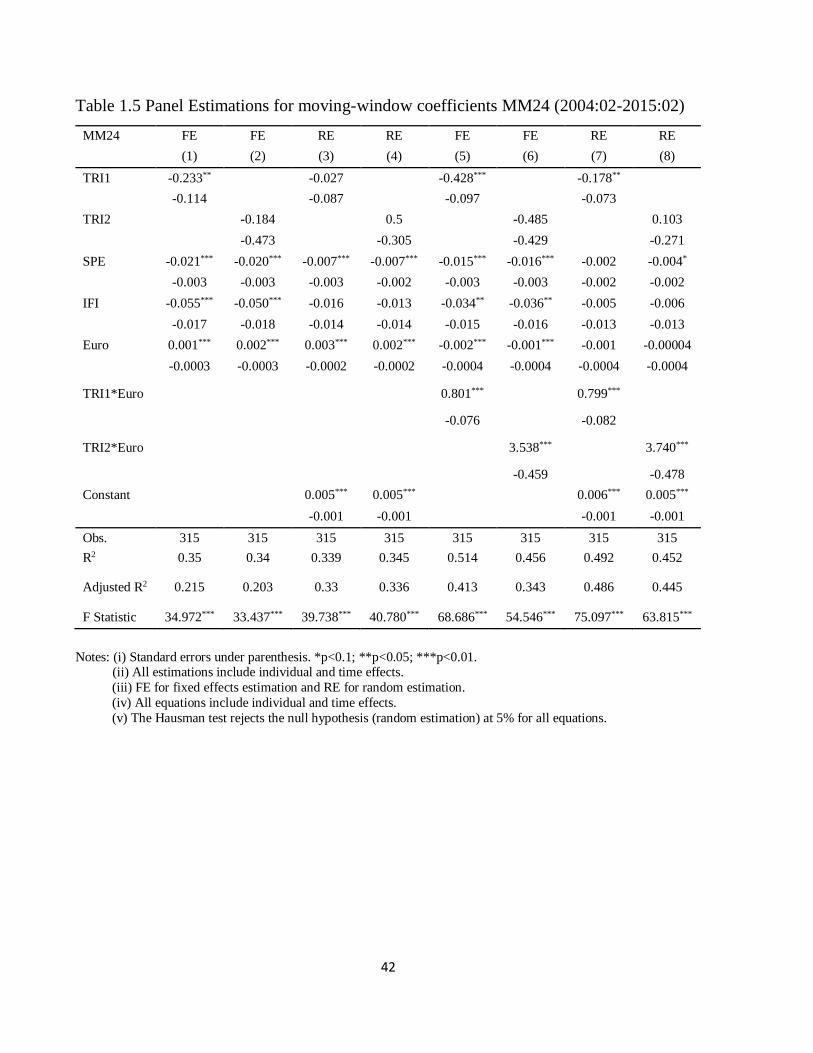
42
Table 1.5 Panel Estimations for moving-window coefficients MM24 (2004:02-2015:02)
MM24 FE FE RE RE FE FE RE RE
(1) (2) (3) (4) (5) (6) (7) (8)
TRI1 -0.233** -0.027 -0.428*** -0.178**
-0.114 -0.087 -0.097 -0.073
TRI2 -0.184 0.5 -0.485 0.103
-0.473 -0.305 -0.429 -0.271
SPE -0.021*** -0.020*** -0.007*** -0.007*** -0.015*** -0.016*** -0.002 -0.004*
-0.003 -0.003 -0.003 -0.002 -0.003 -0.003 -0.002 -0.002
IFI -0.055*** -0.050*** -0.016 -0.013 -0.034** -0.036** -0.005 -0.006
-0.017 -0.018 -0.014 -0.014 -0.015 -0.016 -0.013 -0.013
Euro 0.001*** 0.002*** 0.003*** 0.002*** -0.002*** -0.001*** -0.001 -0.00004
-0.0003 -0.0003 -0.0002 -0.0002 -0.0004 -0.0004 -0.0004 -0.0004
TRI1*Euro 0.801*** 0.799***
-0.076 -0.082
TRI2*Euro 3.538*** 3.740***
-0.459 -0.478
Constant 0.005*** 0.005*** 0.006*** 0.005***
-0.001 -0.001 -0.001 -0.001
Obs. 315 315 315 315 315 315 315 315
R2 0.35 0.34 0.339 0.345 0.514 0.456 0.492 0.452
Adjusted R2 0.215 0.203 0.33 0.336 0.413 0.343 0.486 0.445
F Statistic 34.972*** 33.437*** 39.738*** 40.780*** 68.686*** 54.546*** 75.097*** 63.815***
Notes: (i) Standard errors under parenthesis. *p<0.1; **p<0.05; ***p<0.01.
(ii) All estimations include individual and time effects.
(iii) FE for fixed effects estimation and RE for random estimation.
(iv) All equations include individual and time effects.
(v) The Hausman test rejects the null hypothesis (random estimation) at 5% for all equations.

43
1.5. Conclusion
Since the enlargement of the European Union in 2004, the degree of integration of the
CEECs has been at the center of many debates. Even if Stanisic (2013) rejects the
hypothesis of a common business cycle between CEECs, their fluctuations seem to have
become closer and closer to those of the EA (Di Giorgio, 2016). Some CEECs have already
adopted the euro while others are still candidates. Thus, it was important to determine if
entering the EU and adopting the euro lead to a high degree of interdependency.
Relying on a near-VAR model to capture macroeconomic relationships for seven
CEECs and twelve EA countries, our empirical results indicate that i) CEECs countries are
more affected by EA shocks after the enlargement in 2004 than before. This result could
explain the path of convergence of CEE national business cycles toward those of the EA
observed by Stanisic (2013).
Furthermore, we also find ii) that Germany, France and Italy explain a large part of
economic disturbances in the CEECs-7 resulting from the EA-12. Germany, France and
Italy explain up to 89%, 71% and 69%, respectively, of direct and indirect diffusion of a
shock in the EA. This result is in line with Aguiar-Conraria and Soares (2011) and Belke
et al. (2016): they find that France and Germany, the core of the EA, are the most
synchronized countries with the rest of Europe.
Finally, iii) after the enlargement in 2004, the degree of economic integration
increased more for CEECs that have adopted the euro than the other CEECs. Multiplier
effects of CEECs from EA-12 disturbances have been multiplied by 9.0 and 7.4 after 2004
for Slovakia and Estonia (which have adopted the euro in 2009 and 2011 respectively) and
only by 1.4 and 1.5 for Lithuania and Hungary, for example. Our results are in line with
Frankel and Rose (1998), Rose (2000), Koopman and Azevedo (2008), and Furceri and
Karras (2008): the euro contributes positively to business cycle synchronization. To test for
this “euro effect”, we have simulated moving-window multiplier effects (MM24) and we
have explained those coefficients by trade intensity, industrial specialization, financial
integration, a euro dummy and an interaction term (trade intensity and euro). Results

44
confirm the negative effect of specialization and financial integration but show positive
effects of trade only in the context of the euro adoption. The lack of exchange rate volatility,
development of intra-industry trade and contagion of “animal spirit” constitute arguments
in favor of positive effects of trade inside a currency area. These results suggest that, macro-
economically, countries that have not been adopted the euro yet should do it as soon as
possible and do not wait for a higher level of business cycle synchronization. For further
research, it mays be interesting to consider the role played by the structure of trade (intra-
and inter-industry) within and outside the EA in this opposite effect of trade.
This chapter focuses on the demand-supply spillover channel (Backus et al., 1995)
through which bilateral trade increases the business cycle interdependences. This channel
indicates that trade intensity has positive impacts on the business cycle synchronization.
Following a positive shock, domestic economy (founding members of the euro area in this
chapter) demands more (intermediate) goods from foreign economies (CEE countries). The
positive shock is thereby transmitted to trading partners and the business cycles are more
synchronized. The existing literature also documents other trade channels of macro
fluctuation transmission: resource-shifting, technology transmission and the terms-of-trade
effects. Resource-shifting mechanism is documented in Backus et al., (1992) and predict a
negative impact of trade. When domestic economy experiences a positive productivity
shock, it becomes more productive than its trading partners and therefore attracts the
resources from both itself and foreign countries. This reallocation effect increases domestic
production, decreases foreign production and thereby dampens the synchronization.
Technology transmission channel is highlighted in Liao and Santacreu (2015). According
to the authors, bilateral trade enhances the business cycle comovement through increasing
the productivity comovement. They find that the extensive margin of trade transmits the
technology and knowledge across countries. In addition to these channels, another effect of
trade on business cycle synchronization discussed in the existing literature, as noted in Liao
and Santacreu (2015), is the terms-of-trade effect. Following a positive productivity shock,
domestic goods are cheaper and thus more competitive in the international markets. That

45
decreases the output of trading partner and therefore dampens the comovement. However,
the synchronization may be enhanced because trading partners also benefit from cheaper
imported goods to increase their production. This terms-of-trade effect thus has an
ambiguous sign. Thus, the positive impacts of trade on output correlation may be explained
by the demand-supply spillover, technology transmission and the terms-of-trade
mechanisms. The next chapter contributes to understand more deeply the trade-
comovement puzzle by focusing on two later mechanisms of trade.

46
References
Abeysinghe, T., Forbes, K., 2005. Trade linkages and output-multiplier effects: a structural
VAR approach with a focus on Asia. Rev. Int. Econ. 13 (2), 356–375.
Aguiar-Conraria L. and Soares M. J. 2011. ‘Business Cycle Synchronization and the Euro:
A Wavelet Analysis’. Journal of Macroeconomics, vol. 33(3), pages 477-489.
Artis M. J., Fidrmuc J., and Scharler J., 2008. The transmission of business cycles. The
Economics of Transition, The European Bank for Reconstruction and Development, vol.
16(3), pages 559-582, 07.
Backus, D., Kehoe, P., Kydland, F., 1992. International real business cycles. Journal of
Political Economy 100 (4), 745–775.
Backus, D., Kehoe, P., Kydland, F., 1995. International business cycles: theory vs.
evidence. Frontiers of Business Cycle Research. Princeton University Press.
Baxter M. and Kouparitsas, M. A., 2003. Trade Structure, Industrial Structure, and
International Business Cycles. American Economic Review, American Economic
Association, vol. 93(2), pages 51-56, May.
Baxter M. and Kouparitsas, M. A., 2005. Determinants of business cycle comove- ment: a
robust analysis. Journal of Monetary Economics, Elsevier, vol. 52(1), pages 113-157,
January.
Belke, A., Domnick, C., and Gros D. (2016). Business cycle synchronization in the EMU:
Core vs. periphery. Ruhr Economic Papers 659, RWI - Leibniz-Institut für
Wirtschaftsforschung, Ruhr-University Bochum, TU Dortmund University, University
of Duisburg-Essen.
Boone, L. and Maurel, M., 1999. An Optimal Currency Area Perspective of the EU
Enlargement to the CEECs,’ CEPR Discussion Papers 2119, C.E.P.R. Discussion
Papers.
Clark T. E. and van Wincoop, E., 2001. Borders and business cycles. Journal of
International Economics, Elsevier, vol. 55(1), pages 59-85, October.

47
Dées S. and Zorell N., 2012. Business Cycle Synchronisation: Disentangling Trade and
Financial Linkages. Open Economies Review, Springer, vol. 23(4), pages 623-643,
September.
De Grauwe, P. 1997. The Economics of Monetary Integration, 3rd. ed., Oxford University
Press, London.
De Grauwe P. and Ji Y., 2016. Animal Spirits and the International Transmission of
Business Cycles. CESifo Working Paper Series 5810, CESifo Group Munich.
Di Giorgio C., 2016. Business Cycle Synchronization of CEECs with the euro area: A
Regime Switching Approach. Journal of Common Market Studies, vol. 54(2), pages
284–300.
Dungey, M., Khan, F. and Raghavan, M., 2018. International trade and the transmission of
shocks: The case of ASEAN-4 and NIE-4 economies. Economic Modelling, Elsevier,
vol. 72(C), pages 109-121.
Fidrmuc, J. and Korhonen, I., 2003. Similarity of supply and demand shocks between the
euro area and the CEECs. Economic Systems, Elsevier, vol. 27(3), pages 313-334,
September.
Fidrmuc, J. and Korhonen, I, 2006. Meta-Analysis of the Business Cycle Correlation
between the euro area and the CEECs. Journal of Comparative Economics, Elsevier,
vol. 34(3), pages 518-537, September.
Frankel, J. A. and Rose, A. K., 1998. ‘The Endogeneity of the Optimum Currency Area
Criteria,’ Economic Journal, Royal Economic Society, vol. 108(449), pages 1009-25,
July.
Furceri D. and Karras G., 2008. Business-Cycle Synchronization in the EMU. Applied
Economics, vol. 40(12), pages 1491-1501.
Gonçalves, C. E. S. and Rodrigues, M. and Soares, T., 2009. Correlation of business cycles
in the euro zone. Economics Letters, Elsevier, vol. 102(1), pages 56-58, January.

48
Gouveia S., and Correia L., 2013. Trade Integration and Business Cycle Synchronization
in the euro area: The Case of Southern European Countries. Journal of Economic
Integration, Center for Economic Integration, Sejong University, vol. 28, pages 85-107.
Herwartz, H. and Weber, H., 2013. The role of cross-sectional heterogeneity for magnitude
and timing of the euro's trade effect. Journal of International Money and Finance,
Elsevier, vol. 37(C), pages 48-74.
Imbs J., 2004. Trade, Finance, Specialization and Synchronization. The Review of
Economics and Statistics, MIT Press, vol. 86(3), pages 723-734, August.
Inklaar, Robert, Jong-A-Pin, Richard, de Haan, Jakob, 2008. Trade and business cycle
synchronization in OECD countries--A re-examination. European Economic Review,
Elsevier, vol. 52(4), pages 646-666, May.
IMF (2012), 2012 Spillover Report, Washington.
Jimenez-Rodríguez R., Morales-Zumaquero A. and Egert B., 2010. The effect of Foreign
Shocks in Central and Eastern Europe. Journal of Policy Modeling, 32 461–477
Jimenez-Rodríguez R., Morales-Zumaquero A. and Egert B., 2013. Business Cycle
Synchronization between Euro Area and Central and Eastern European Countries.
Review of Development Economics, 17(2) 379–395
Kenen P., 1969. The Theory of Optimum Currency Areas: An Eclectic View in Mundell
and Swoboda (eds.) Monetary Problems in the International Economy, University of
Chicago Press, Chicago.
Keppel C. and Prettner K., 2015. How interdependent are eastern European economies and
the euro area? The Quarterly Review of Economics and Finance, Elsevier, vol. 58(C),
pages 18-31.
Koopman S. J. and Azevedo J. V., 2008. Measuring Synchronization and Convergence of
Business Cycles for the euro area, UK and US. Oxford Bulletin of Economics and
Statistics, vol. 70(1), pages 23-51.
49
Korhonen I., 2003. Some empirical tests on the integration of economic activity between
the euro area and the accession countries. The Economics of Transition, The European
Bank for Reconstruction and Development, vol. 11(1), pages 177-196, March.
Krugman P. R., 1993. Lessons of Massachusetts for EMU in Adjustment and growth in the
European Monetary Union, Cambridge University Press, F. Torres, F. Giavazzi (eds),
p.241-69.
Liao, W., Santacreu, A.M., 2015. The trade-comovement puzzle and the margins of
international trade. Journal of International Economics, Volume 96, Issue 2, July 2015,
Pages 266-288, ISSN 0022-1996
McKinnon, R., 1963. Optimum Currency Area. American Economic Review, September,
pp. 717-725.
Mundell, R. A., 1961. A theory of optimum currency area. American Economic Review, 51,
657–665.
Robert, A., Baldwin, R. and Taglioni, D., 2007. The impact of monetary union on trade
prices. Journal of Financial Transformation, Capco Institute, vol. 19, pages 35-48.
Rose A. K., 2000. One money, one market: the effect of common currencies on trade.
Economic Policy, CEPR; CES; MSH, vol. 15(30), pages 7-46, 04.
Siedschlag I., 2010. Patterns and determinants of business cycle synchronization in the
enlarged European Economic and Monetary Union. Eastern Journal of European
Studies, Centre for European Studies, AlexandruIoan Cuza University, vol. 1, pages 21-
44, June.
Stanisic N., 2013. Convergence between the business cycles of Central and Eastern
European countries and the euro area. Baltic Journal of Economics, Baltic International
Centre for Economic Policy Studies, vol. 13(1), pages 63-74, July.
Wang J. and Zivot E., 2000. A Bayesian Time Series Model of Multiple Structural Changes
in Level, Trend and Variance. Journal of Business and Economics, 18: 374-386.

50
Appendix
Table 1.A.1 Model specification tests
Country Jan 1996-Sep 2015 Pre-accession model Post-accession model
LAGs LB JB AIC LAGs LB JB AIC LAGs LB JB AIC
CZE (2,2,7) 0.36 0.03 -463.10 (1,2,2) 0.46 0.18 -238.36 (3,1,11) 0.19 0.82 -363.61
EST (2,2,7) 0.38 0.03 -396.00 (1,1,1) 0.11 0.90 -221.80 (8,3,5) 0.93 0.02 -299.65
HUN (2,3,8) 0.94 0.00 -502.82 (2,3,1) 0.06 0.41 -271.76 (2,1,7) 0.43 0.00 -372.33
POL (1,1,1) 0.08 0.00 -571.99 (2,3,3) 0.55 0.28 -277.70 (2,1,7) 0.42 0.55 -468.57
SVK (1,1,1) 0.71 0.00 -350.76 (3,1,5) 0.27 0.22 -256.14 (2,1,7) 0.17 0.02 -258.18
SVN (8,5,11) 0.05 0.00 -542.21 (3,3,1) 0.42 0.00 -306.86 (2,2,5) 0.53 0.00 -397.06
LTU (7,1,1) 0.99 0.00 -87.65 (3,4,1) 0.29 0.87 -60.52 (10,6,1) 0.74 0.00 -164.00
AUT (5,5,11) 0.50 0.00 -669.48 (12,3,3) 0.60 0.01 -320.20 (2,2,9) 0.74 0.96 -472.35
BEL (4,3,4) 0.87 0.00 -576.11 (2,3,7) 0.71 0.00 -340.90 (3,4,7) 0.39 0.93 -399.44
FIN (2,3,8) 0.11 0.00 -612.06 (6,6,3) 0.42 0.48 -350.13 (2,1,7) 0.66 0.00 -399.34
FRA (3,3,12) 0.59 0.02 -826.19 (6,2,1) 0.53 0.00 -431.70 (2,2,9) 0.39 0.23 -537.94
DEU (2,3,8) 0.74 0.77 -751.54 (4,1,5) 0.05 0.62 -416.51 (1,3,1) 0.32 0.12 -475.01
IRL (3,1,10) 0.14 0.00 -105.91 (3,2,10) 0.55 0.44 -149.49 (3,5,7) 0.21 0.00 -109.49
ITA (2,3,8) 0.44 0.39 -822.26 (1,3,2) 0.83 0.07 -463.94 (3,3,2) 0.20 0.44 -531.01
LUX (3,2,11) 0.25 0.00 -304.83 (6,2,5) 0.60 0.00 -187.54 (2,2,9) 0.56 0.00 -245.11
NLD (3,3,12) 0.16 0.16 -541.36 (3,4,12) 0.74 0.46 -317.86 (1,1,1) 0.13 0.81 -368.08
PRT (3,3,12) 0.78 0.98 -529.89 (2,2,5) 0.95 0.06 -308.49 (2,1,3) 0.19 0.76 -398.43
GRC (10,4,1) 0.06 0.00 -477.86 (2,2,5) 0.62 0.00 -285.99 (4,0,1) 0.11 0.39 -358.25
ESP (6,3,8) 0.11 0.00 -720.66 (2,2,5) 0.55 0.01 -410.04 (1,1,2) 0.08 0.38 -524.90
Notes: (i) LB, JB denote p-value of Ljung-Box test and Jarque-Berra test, respectively.
(ii) LAGs represent lags of national output (y), international output (ye) and rest of the word’s output.
(iii) AIC refers to Akaike Information Criterion.
(iv) Country code: AUT: Austria, BEL: Belgium, FIN: Finland, FRA: France, GER: Germany, GRC: Greece,
IRL: Ireland, ITA: Italia, LUX: Luxembourg, NLD: Netherlands, PRT: Portugal, SPA: Spain, EST: Estonia, HUN: Hungary, LTU: Lithuania, POL: Poland, CZE: Republic Czech, SVK: Slovakia, SVN: Slovenia.
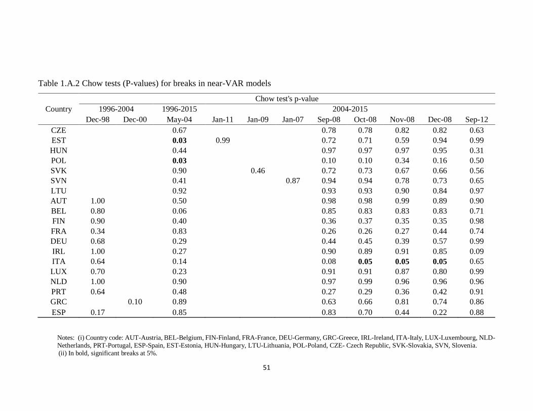
51
Table 1.A.2 Chow tests (P-values) for breaks in near-VAR models
Country
Chow test's p-value
1996-2004 1996-2015 2004-2015
Dec-98 Dec-00 May-04 Jan-11 Jan-09 Jan-07 Sep-08 Oct-08 Nov-08 Dec-08 Sep-12
CZE 0.67 0.78 0.78 0.82 0.82 0.63
EST 0.03 0.99 0.72 0.71 0.59 0.94 0.99
HUN 0.44 0.97 0.97 0.97 0.95 0.31
POL 0.03 0.10 0.10 0.34 0.16 0.50
SVK 0.90 0.46 0.72 0.73 0.67 0.66 0.56
SVN 0.41 0.87 0.94 0.94 0.78 0.73 0.65
LTU 0.92 0.93 0.93 0.90 0.84 0.97
AUT 1.00 0.50 0.98 0.98 0.99 0.89 0.90
BEL 0.80 0.06 0.85 0.83 0.83 0.83 0.71
FIN 0.90 0.40 0.36 0.37 0.35 0.35 0.98
FRA 0.34 0.83 0.26 0.26 0.27 0.44 0.74
DEU 0.68 0.29 0.44 0.45 0.39 0.57 0.99
IRL 1.00 0.27 0.90 0.89 0.91 0.85 0.09
ITA 0.64 0.14 0.08 0.05 0.05 0.05 0.65
LUX 0.70 0.23 0.91 0.91 0.87 0.80 0.99
NLD 1.00 0.90 0.97 0.99 0.96 0.96 0.96
PRT 0.64 0.48 0.27 0.29 0.36 0.42 0.91
GRC 0.10 0.89 0.63 0.66 0.81 0.74 0.86
ESP 0.17 0.85 0.83 0.70 0.44 0.22 0.88
Notes: (i) Country code: AUT-Austria, BEL-Belgium, FIN-Finland, FRA-France, DEU-Germany, GRC-Greece, IRL-Ireland, ITA-Italy, LUX-Luxembourg, NLD-
Netherlands, PRT-Portugal, ESP-Spain, EST-Estonia, HUN-Hungary, LTU-Lithuania, POL-Poland, CZE- Czech Republic, SVK-Slovakia, SVN, Slovenia.
(ii) In bold, significant breaks at 5%.

52
Table 1.A.3 Residual analysis
CZE EST HUN POL SVK SVN LTU AUT BEL FIN
CZE -0.01 0.21 0.38 -0.05 0.15 0.06 0.06 -0.19 0.07
EST 0.01 -0.03 -0.02 0.05 0.18 0.29 0.00 -0.20 -0.25
HUN 0.03 0.05 0.19 0.11 0.12 0.18 -0.04 -0.14 -0.13
POL -0.01 0.07 0.27 -0.06 0.21 0.01 -0.09 -0.02 -0.09
SVK 0.03 -0.09 -0.17 0.13 0.26 0.08 -0.17 -0.06 -0.05
SVN -0.08 -0.19 0.06 -0.06 0.05 0.01 -0.13 -0.20 -0.16
LTU 0.12 -0.12 0.01 -0.23 -0.05 0.04 -0.09 0.02 -0.09
AUT -0.02 0.01 0.09 0.16 0.06 -0.06 -0.01 0.11 -0.06
BEL -0.19 0.09 0.03 0.16 -0.04 -0.24 -0.02 -0.01 -0.01
FIN 0.11 -0.37 -0.04 0.06 0.27 0.10 -0.06 -0.21 -0.08
FRA 0.29 0.13 -0.09 -0.13 -0.01 0.09 0.23 0.03 -0.11 -0.07
DEU -0.32 0.12 -0.05 -0.21 -0.35 0.15 -0.06 -0.12 -0.11 -0.14
IRL 0.02 -0.07 0.11 -0.04 -0.09 0.02 0.08 -0.13 -0.18 0.07
ITA -0.09 0.15 -0.01 0.22 -0.04 -0.13 -0.08 -0.05 0.06 0.05
LUX -0.04 -0.01 0.01 -0.13 0.08 0.25 0.00 -0.14 -0.25 0.08
NLD 0.06 0.06 0.03 -0.13 0.08 0.08 0.15 -0.02 -0.10 0.05
PRT -0.12 0.08 -0.01 0.10 0.13 0.08 -0.10 -0.06 0.04 -0.07
GRC 0.13 -0.08 -0.04 0.08 0.16 -0.08 -0.11 0.08 -0.17 0.05
ESP -0.03 -0.13 0.04 -0.05 0.12 0.04 0.11 0.01 0.01 0.07
FRA DEU IRL ITA LUX NLD PRT GRC ESP
CZE -0.13 -0.10 0.07 0.18 0.21 0.18 0.17 -0.11 0.01
EST 0.22 -0.21 -0.13 -0.05 0.04 0.17 0.11 0.22 0.05
HUN -0.14 0.10 -0.12 0.10 -0.17 -0.19 -0.04 0.07 0.07
POL -0.18 -0.01 -0.13 0.13 0.24 0.04 0.00 -0.05 -0.13
SVK -0.11 0.32 -0.29 -0.14 0.04 -0.23 -0.01 -0.20 0.18
SVN 0.09 0.15 -0.04 0.01 0.08 0.17 -0.08 -0.08 0.08
LTU 0.13 -0.18 -0.04 -0.08 -0.03 0.15 -0.03 0.00 -0.07
AUT 0.20 -0.47 -0.02 0.08 0.14 0.26 0.08 -0.01 -0.30
BEL -0.34 -0.15 -0.09 -0.01 -0.04 -0.19 -0.05 -0.13 -0.07
FIN -0.04 0.08 0.05 -0.13 0.01 0.16 0.24 -0.12 -0.03
FRA -0.33 0.01 -0.13 0.03 0.39 0.00 -0.14 -0.21
DEU -0.24 -0.01 -0.26 -0.23 -0.27 -0.13 -0.23 0.20
IRL -0.01 0.01 -0.04 0.11 0.12 -0.12 0.10 -0.03
ITA -0.19 -0.18 -0.10 0.12 0.03 -0.07 0.01 -0.31
LUX 0.07 0.04 0.06 -0.05 0.14 -0.03 -0.12 -0.21
NLD 0.37 -0.09 0.06 -0.06 0.10 0.02 -0.12 -0.24
PRT -0.21 0.11 0.12 0.07 -0.13 -0.23 -0.24 -0.04
GRC -0.04 -0.29 0.08 -0.02 0.20 0.02 -0.25 0.15
ESP 0.10 -0.08 0.20 -0.22 0.14 0.13 -0.12 0.15
Notes: Lower triangular matrix consists of correlations of residuals from the post-accession model. Upper triangular
matrix consists of correlations of residuals from the pre-accession model. Country code: AUT: Austria, BEL: Belgium,
FIN: Finland, FRA: France, DEU: Germany, GRC: Greece, IRL: Ireland, ITA: Italia, LUX: Luxembourg, NLD:
Netherlands, PRT: Portugal, ESP: Spain, EST: Estonia, HUN: Hungary, LTU: Lithuania, POL: Poland, CZE: Republic Czech, SVK: Slovakia, SVN: Slovenia. In bold, correlations larger than 0.30.

53
Table 1.A.4 Multiplier effects before and after the accession (in percent)
CZE EST HUN POL
Pre-2004 Post-2004 Pre-2004 Post-2004 Pre-2004 Post-2004 Pre-2004 Post-2004
AUT 0.22 0.55 0.17 0.70 0.57 0.41 0.23 0.52
BEL 0.32 0.92 0.31 1.33 0.76 0.67 0.37 0.91
FIN 0.03 0.27 0.14 1.45 0.08 0.20 0.04 0.28 FRA 0.39 1.38 0.38 1.94 0.93 1.01 0.45 1.38
DEU 0.73 4.60 0.65 6.19 1.70 3.35 0.82 4.52
IRL 0.14 0.33 0.14 0.49 0.32 0.24 0.15 0.33
ITA 0.35 1.22 0.33 1.71 0.82 0.91 0.40 1.23 LUX 0.10 0.21 0.09 0.28 0.23 0.15 0.11 0.20
NLD 0.45 2.15 0.46 3.26 1.08 1.57 0.52 2.16
PRT 0.14 0.38 0.14 0.53 0.34 0.28 0.17 0.38 ESP 0.26 1.16 0.25 1.65 0.61 0.86 0.30 1.16
GRC 0.09 0.22 0.09 0.32 0.21 0.17 0.10 0.22
SVK SVN LTU
Pre-2004 Post-2004 Pre-2004 Post-2004 Pre-2004 Post-2004
AUT 0.19 0.85 0.25 0.65 0.43 0.34
BEL 0.27 1.39 0.35 1.00 0.82 0.64
FIN 0.03 0.42 0.04 0.29 0.11 0.30
FRA 0.33 2.12 0.46 1.56 1.01 0.95
DEU 0.6 6.92 0.8 4.95 1.71 3.03
IRL 0.11 0.49 0.14 0.36 0.36 0.24
ITA 0.3 1.89 0.43 1.47 0.86 0.83
LUX 0.08 0.31 0.11 0.23 0.24 0.14
NLD 0.37 3.28 0.49 2.32 1.16 1.53
PRT 0.12 0.58 0.16 0.42 0.36 0.26
ESP 0.21 1.78 0.29 1.29 0.66 0.80
GRC 0.07 0.34 0.1 0.25 0.22 0.15
Notes: This table presents the cumulative impulse response in 24 months ahead of country in column to a shock
originated in country in row. Country code: AUT: Austria, BEL: Belgium, FIN: Finland, FRA: France, DEU: Germany,
GRC: Greece, IRL: Ireland, ITA: Italia, LUX: Luxembourg, NLD: Netherlands, PRT: Portugal, ESP: Spain, EST:
Estonia, HUN: Hungary, LTU: Lithuania, POL: Poland, CZE: Republic Czech, SVK: Slovakia, SVN: Slovenia.

54
CHAPTER 2
EXTENSIVE MARGIN AND TRADE-COMOVEMENT
PUZZLE
Highlights
The trade-comovement puzzle has been highlighted by Kose and Yi (2006), who have
suggested that theoretical models find weak effects of trade on business cycle correlations.
To explain this puzzle, Juvenal and Santos-Monteiro (2017) have divided output
comovement into three factors: correlation between each country's TFP, correlation
between each country's share of expenditure on domestic goods, and correlation between
each country’s TFP and the partner’s share of expenditure on domestic goods. From this
decomposition, they have revealed that the trade-comovement puzzle arises mainly from
the second factor. As such, in their theoretical model, trade decreases the correlation
between each country's share of expenditure on domestic goods because the model
generates a countercyclical terms-of-trade. To investigate this counterfactual effect, we
decompose trade intensity into intensive and extensive margins. We then study the
effects of each margin on three component factors of output comovement. Using data for
40 countries (24 developed countries and 16 developing countries) over the period 1990-
2015, we find that the effects of the intensive margin on comovements are ambiguous.
However, the extensive margin increases not only the correlation of TFP between trading
partners (first factor) but also the correlation between each country's shares of domestic
goods (second factor). This result emphasizes that new exported products transmit TFP
shocks and do not deteriorate but instead improve the terms-of-trade. The extensive
margin of trade should be integrated into theoretical model to solve the puzzle.
JEL Classifications: F14, F41, F44, E32
Keywords: Business cycle comovement, Trade-comovement puzzle, Trade Margins

55
2.1. Introduction and Literature Review
Although substantial empirical evidence has suggested that bilateral trade contributes
positively to output comovement (Frankel and Rose, 1998; Clark and Wincoop, 2001;
Imbs, 2004, Baxter and Kouparitsas, 2005, among others), theoretical models fail to fully
replicate this relationship. International business cycle models are unable to generate trade
effects on business cycles synchronization as strong as those observed from the data.
Kose and Yi (2006) have developed an international business cycle model and
simulated the effects of increased trade integration on business cycle correlations. Their
model implies an increase in output correlation for pairs of countries with stronger
trade linkages. However, this theoretical correlation accounts for approximately one tenth
of the empirically detected effect. They have named this fact the trade-comovement
puzzle in the standard international real business cycle model. The authors have also
highlighted that when allowing for higher TFP shock comovement, the model performance
improves in reducing the gap between empirical findings and theoretical predictions.
To solve this trade-comovement puzzle, Arkolakis and Ramanarayanan (2009) have
used an international business cycle model with two stages of production. Bilateral trade
varies with trade barriers. The results have suggested that vertical specialization fails to
solve the trade-comovement puzzle with perfect competition but has helped solve the
puzzle with imperfect competition. Di Giovanni and Levchenko (2010), using firm-level
data and input-output matrix, have indicated a higher comovement for sectors that trade
more with each other, in terms of volume and frequency. They have noted that vertical
production linkages are responsible for 30 percent of total trade effect. Wong and Eng
(2013) have developed a model with three production stages, which allow for vertical trade
(importing intermediates for re-exporting as intermediates) and processing trade (importing
intermediates for re-exporting as final goods). The authors have demonstrated that their
model can solve the puzzle. Johnson (2014) has included input-output linkages across
sectors into international real business cycle model. Their results have indicated that the
puzzle cannot solved by input trade: “the model yields high trade-comovement correlations

56
for goods, but near-zero correlations for services and thus low aggregate correlations.”
For Liao and Santacreu (2015), theoretical effects of trade on business cycle
comovement can be increased if TFP correlation is considered. Distinguishing between
intensive and extensive margins of trade, Liao and Santacreu (2015) have revealed that the
extensive margin of trade increases correlation between the trading partner’s aggregate
productivity and therefore drives the observed output comovement. In addition, business
cycles between countries that trade a wider variety should be highly correlated. Zlate (2016)
has examined the effect of offshoring through vertical foreign direct investments on
business cycle correlation. His model has distinguished between intensive and extensive
margins of offshoring, indicating that offshoring and its extensive margin raise output
comovement across countries. More recently, Drozd et al. (2017) have studied the dynamic
properties of trade elasticity. They have argued that models will be more consistent with
dynamic instead of static trade elasticity.
According to Juvenal and Santos-Monteiro (2017), business cycle comovement
could be explained by three factors in most theoretical models: correlation between each
country’s TFP, correlation between each country’s share of expenditure on domestic goods
and correlation between each country’s TFP and its trading partner’s share of expenditure
on domestic goods. Juvenal and Santos-Monteiro (2017) have illustrated that the trade-
comovement puzzle is explained by the second factor. This counterfactual effect results
from the fact that TFP shocks induce a deterioration of the domestic terms-of-trade and that
the second factor responds more strongly to terms-of-trade variations when countries are
more trade-integrated.
In this chapter, we evaluate the effects of the extensive margin and the intensive
margin of trade on the three aforementioned component factors. While Juvenal and Santos-
Monteiro (2017) have examined the effects of total trade, we focus on the effects of
margins of trade on component factors. Our hypothesis holds that extensive margin has a
positive impact on TFP correlations (first factor) and also has a positive effect on the
correlation between each country's shares of domestic goods (second factor). In the last
case, the terms-of-trade are procyclical if we consider the extensive margin of trade.

57
By using a sample that covers 40 countries, we first follow the work of Juvenal and
Santos-Monteiro (2017) and acknowledge that business comovements are mainly
explained by correlations of TFP and shares of expenditure on domestic goods, whereas
the effect of the third factor is ambiguous. Second, our results reveal that the extensive
margin of trade not only increases the correlation of TFP between trading partners (Liao
and Santacreu, 2015) but also increases the correlation between each country's shares of
domestic goods. In contrast, the effects of the intensive margin are negative or
insignificant. These results emphasize that new exported products transmit TFP shocks via
embedded technology information, and more importantly, they do not deteriorate the
terms-of-trade. The higher level of the extensive margin of trade between two countries is,
the more the TFP, the share of expenditure on domestic goods and therefore the output
between these countries commove. Thus, to solve the trade-comovement puzzle,
theoretical models should integrate the extensive margin of trade.
The remainder of this chapter is divided into four sections. Section 2.2 presents the
methodology, data and measurements. Next, section 2.3 describes the results. Lastly,
section 2.4 presents robustness checks, while section 2.5 concludes the chapter.
2.2. Methodology, Data and Measurement
First, we explain the correlation of output fluctuations by addressing the three component
factors proposed by Juvenal and Santos-Monteiro (2017):
𝑐𝑜𝑟𝑟(𝑦��, 𝑦��) = 𝑏01 + 𝑏11 𝑐𝑜𝑟𝑟(𝐴��, 𝐴��)+𝑏21 𝑐𝑜𝑟𝑟(𝜆��, 𝜆��)+𝑏31 𝑐𝑜𝑟𝑟(𝜆��, 𝐴��)+ 𝜀𝑖𝑗1 (2.1)
where 𝑐𝑜𝑟𝑟(𝑦��, 𝑦��) denotes the correlation between each country’s output, 𝑐𝑜𝑟𝑟(𝐴��, 𝐴��) is
the correlation between each country's TFP, 𝑐𝑜𝑟𝑟(𝜆��, 𝜆��) refers to the correlation between
each country's share of expenditure on domestic goods, and 𝑐𝑜𝑟𝑟(𝜆��, 𝐴��) is the correlation
between each country’s TFP and the trading partner’s share of expenditure on domestic
goods.
58
The data concern 40 countries, including 24 developed countries and 16 developing
countries, over the period 1990-2015. The developed countries are Australia, Austria,
Canada, Denmark, Finland, France, Germany, Greece, Hungary, Iceland, Ireland, Italy,
Japan, South Korea, the Netherlands, New Zealand, Norway, Poland, Portugal, Spain,
Sweden, Switzerland, United Kingdom and the United States. The developing countries
consist of Chile, China, Indonesia, India, Malaysia, Philippines, Argentina, Brazil, Mexico,
Turkey, Costa Rica, Romania, Thailand, Uruguay, Bulgaria and Tunisia. This sample
accounts for 78% of world trade and 86% of world GDP. The data have been extracted
from various databases, as detailed below.
Business cycle comovement is defined as the correlation of the cyclical components
of real GDP (in millions, local currencies) from 1990 to 2015. The series are detrended by
the Hodrick-Prescott (HP) filter. For the OECD countries, the data come from the OECD
database, and for the non-OECD countries, the nominal output in local currency is
extracted from the World Bank database and is then deflated by the GDP deflator (base
year 2010), which has been obtained from the International Financial Statistics (IMF).
The correlation between each country's TFP is calculated from the series of TFP,
which are also detrended by the HP filter. We follow Liao and Santacreu (2015) in
estimating the productivity aggregate of country i in year t:
)()1()()()( itititit KLogLLogYLogTFPLog
where Yit denotes real GDP in local currency, Kit is the physical capital stock and Lit
is the total employment. The employment data comes from the IMF and World Bank
databases, while the series of physical capital stock are constructed using the perpetual
inventory method. We assume an annual depreciation of 10%, and the initial capital stock
is zero. In addition, following the literature, α is set to 0.64 for all countries. The data of
real gross fixed capital formation is extracted from the Word Bank database. This method
is similar to the one used by Liao and Santacreu (2015).
The share of expenditure on domestic goods corresponds to the share of domestic
intermediate goods used to produce final goods. As in the work of Juvenal and Santos-

59
Monteiro (2017), share of expenditure on domestic goods is defined as one minus the
import penetration ratio, or
iii
ii
iii
i
iMXGDP
XGDP
MXGDP
M
1
where Xi and Mi denote the total exports and imports, respectively, of country i. The
total export and total import data is extracted from the Direction of Trade Statistics (IMF)
database. The GDPi is the nominal output, in US dollars, that comes from the OECD
database for OECD countries and the World Bank and IMF databases for non-OECD
countries. We use nominal output in US dollars because the value of exports and imports
are in US current dollar. The series of lambda are then de-trended by the HP filter. The
correlation between each country's share of expenditure on domestic goods is calculated
from the cyclical components over the period 1990–2015.
The third factor identified by Juvenal and Santos-Monteiro (2017) is the sum of the
correlation between cyclical components of TFP of country i and lambda of country j and
the correlation between cyclical components of TFP of country j and lambda of country i.
After examining the component factor structure of output comovement, we revisit
the impacts of trade intensity on business cycle synchronization and its effects on each
component factor by estimating the following equations:
𝑐𝑜𝑟𝑟(𝑦��, 𝑦��) = 𝑏02 + 𝑏12 log(𝑏𝑖𝑙𝑎𝑡𝑒𝑟𝑎𝑙𝑡𝑟𝑎𝑑𝑒)𝑖𝑗 + 𝜀𝑖𝑗2 (2.2)
𝑐𝑜𝑟𝑟(𝐴��, 𝐴��) = 𝑏03 + 𝑏13 log(𝑏𝑖𝑙𝑎𝑡𝑒𝑟𝑎𝑙𝑡𝑟𝑎𝑑𝑒)𝑖𝑗 + 𝜀𝑖𝑗3 (2.3)
𝑐𝑜𝑟𝑟(𝜆��, 𝜆��) = 𝑏04 + 𝑏14 log(𝑏𝑖𝑙𝑎𝑡𝑒𝑟𝑎𝑙𝑡𝑟𝑎𝑑𝑒)𝑖𝑗 + 𝜀𝑖𝑗4 (2.4)
𝑐𝑜𝑟𝑟(𝜆��, 𝐴��) = 𝑏05 + 𝑏15 log(𝑏𝑖𝑙𝑎𝑡𝑒𝑟𝑎𝑙𝑡𝑟𝑎𝑑𝑒)𝑖𝑗 + 𝜀𝑖𝑗5 (2.5)
We consider two traditional measures of bilateral trade intensity. The first indicator
is calculated using only bilateral export and import data:
T
t jtitjtit
tijtij
ijMMXX
MX
Ttrade
1
,,11

60
where Xijt and Mijt refer to the bilateral export and import between country i and j during
the year t, in current US dollars. Thus, Xit, Mit, Xjt and Mjt denote the total exports and
imports of countries i and j, respectively, in year t. The second indicator is defined:
T
t jtit
tijtij
ijYY
MX
Ttrade
1
,,11
where Yit and Yjt are the nominal GDP in current US dollars of countries i and j.
The bilateral trade data is exploited from DOTS (IMF). The series of nominal
output come from the OECD, World Bank and IFS (IMF) databases.
Then, the trade effects are decomposed into the intensive margin IM and the
extensive margin EM:
𝑐𝑜𝑟𝑟(𝑦��, 𝑦��) = 𝑏06 + 𝑏16 𝑙𝑜𝑔(𝐸𝑀)𝑖𝑗 + 𝑏26 𝑙𝑜𝑔(𝐼𝑀)𝑖𝑗 + 𝜀𝑖𝑗6 (2.6)
𝑐𝑜𝑟𝑟(𝐴��, 𝐴��) = 𝑏07 + 𝑏17 𝑙𝑜𝑔(𝐸𝑀)𝑖𝑗 + 𝑏27 𝑙𝑜𝑔(𝐼𝑀)𝑖𝑗 + 𝜀𝑖𝑗7 (2.7)
𝑐𝑜𝑟𝑟(𝜆��, 𝜆��) = 𝑏08 + 𝑏18 𝑙𝑜𝑔(𝐸𝑀)𝑖𝑗 + 𝑏28 𝑙𝑜𝑔(𝐼𝑀)𝑖𝑗 + 𝜀𝑖𝑗8 (2.8)
𝑐𝑜𝑟𝑟(𝜆��, 𝐴��) = 𝑏09 + 𝑏19 𝑙𝑜𝑔(𝐸𝑀)𝑖𝑗 + 𝑏29 𝑙𝑜𝑔(𝐼𝑀)𝑖𝑗 +𝜀𝑖𝑗9 (2.9)
Intensive and extensive margins of trade are obtained from the export decomposition using
the methodology proposed by Hummels and Klenow (2005). The extensive margin of
trade is defined as the ratio of country k’s exports to j in Iij and country k’s exports to j
in I, where Iij is the set of observable goods in which country i has positive export to
country j and I is the set of all goods:
Im
kjm
Im
kjm
ijExport
Export
EMij
The wider the variety of goods that country i exports to country j, the higher the EMij.
The intensive margin of trade compares nominal exports for country i and k in a common
set of varieties. It is constructed as the ratio of country i’s nominal shipments to country j
61
to country k’s nominal shipments to country j in the same set of goods. IMij is higher when
country i exports higher quantities of each product category to j.
ij
ij
Im
kjm
Im
ijm
ijExport
Export
IM
Margins of trade between countries i and j are then computed as the sum of the
natural logarithm of the margins of export of country i to j and those of country j to i:
)()()( jiijij EMLogEMLogEMLog
)()()( jiijij IMLogIMLogIMLog
We also consider an alternative measure of the overall bilateral trade intensity from
the calculation of margins:
)()()( jiijij IMLogEMLogOTLog
The BACI database, which consists of 5,017 six-digit U.N HS product codes from
CEPII (Gaulier and Zignago, 2010), is exploited to calculate the extensive and intensive
margins of trade. We compute EM and IM for each year and then take the average over the
period 1990–2015. The specifications are estimated by the OLS and two-stage least squares
(2SLS) methods. In line with Liao and Santacreu (2015), the distance and the regulation
entry cost are used as instruments to deal with the measurement errors and omitted
variables problem. These authors have argued that the transport cost has a significant
impact on the intensive margin, whereas the extensive margin is affected by the entry cost
that firms must pay to entry into a new market. The distance data is obtained from CEPII,
and the data of regulation entry cost is constructed by Djankov et al. (2002). This variable
is measured by the amount of time and money lost for legal procedures to start operating a
business. Since the bilateral extensive margin is calculated as the sum of the extensive
margins for two countries, we take the sum of regulation entry cost of two countries for
each country pair.
62
2.3. Empirical Results
2.3.1 Stylized Facts
To begin, we examine the evolution of the extensive and intensive margins of trade over
the considered period. Figure 2.1 indicates the averages of the margins of trade of all
country pairs from 1990 to 2015. The extensive margin and intensive margin of trade seem
to move in opposite directions until 1996, at which point they do not produce many
fluctuations. In general, while the intensive margin decreased sharply from 1990 to 1994
and tended to be stable during the remaining period, the extensive margin showed an
increasing trend over the studied period. In fact, the extensive margin of trade temporarily
declined from 2008 to 2013 due to the global crisis and raised again in 2014 and 2015.
Dutt et al. (2013) have used data on exports for 150 countries from 1962–1999 and have
indicated that the growth in overall trade is mainly due to the increase of trade in new
products, or the extensive margin of trade. In fact, two factors over recent decades explain
these movements: technological development helps enterprises create new products and
economic integration in a globalized world helps firms find new exporting markets. Naknoi
(2015) has suggested that the extensive margin of export negatively correlates with the
intensive margin of export for 90% of countries that trade with the US.

63
Figure 2.1 Extensive and intensive margins of trade
Note: The extensive and intensive margins are computed as the average of all pairs of countries.
The descriptive statistics for the variables are presented in Table 2.A.1 in the
appendix. The output correlation of country pairs in our sample has a mean of 0.23 and
varies from -0.71 (Brazil – Ireland) to 0.90 (Austria – Netherlands). The correlation of
TFP between trading partners is always positive, with a mean of 0.78, a minimum of 0.00
(Argentina – Ireland) and a maximum of 0.99 (Austria – Germany). The range of
correlation of the share of expenditure on domestic goods is from -0.63 (Argentina –
Ireland) to 0.89 (United States – Finland). The minimum correlation between each
country’s TFP and the trading partner’s share of expenditure on domestic goods is -1.17
(Austria – Germany), and its maximum is 0.63 (Indonesia – Iceland). As Hummels and
Klenow (2005) have noted, the extensive margin is always larger than the intensive
margin, since the former, in this case, reaches a mean of 0.280. The two countries that
trade the largest number of varieties are Canada and the United States. The opposite case
is Iceland and Uruguay. The intensive margin reaches a maximum with the country pair
Canada – United States and the minimum with Iceland – Mexico.
0.00
0.02
0.04
0.06
0.08
0.10
0.12
0.14
0.16
0.00
0.10
0.20
0.30
0.40
0.50
0.60
1990
19
91
19
92
19
93
19
94
19
95
19
96
19
97
19
98
1999
20
00
20
01
20
02
20
03
20
04
20
05
20
06
20
07
20
08
2009
20
10
20
11
20
12
20
13
20
14
20
15
Exte
nsi
ve m
argi
n
Extensive margin (left axis) Intensive margin (right axis)
64
2.3.2 Business Cycle Comovement Factor Structure
Juvenal and Santos-Monteiro (2017) have used the data of industrial manufacturing from
24 OECD countries and have found that all three factors significantly affect output
correlations. While the comovement between TFP and the shares of expenditure on
domestic goods has positive effects on output correlation, the third factor contributes
negatively and thus reduces the business cycle synchronization. Based upon the data for 40
countries, the results reported in Table 2.1 also indicate that the correlation between TFP
and between shares of expenditure on domestic goods are the main sources of business
cycle comovement. However, unlike Juvenal and Santos-Monteiro (2017) have suggested,
the coefficient of the TFP correlation is larger than that of the correlation of shares of
expenditure on domestic goods in all specifications. Furthermore, we find that the impact
of the correlation between each country’s TFP and the trading partner’s share of
expenditure on domestic goods is not significant. However, excluding this factor from the
benchmark regression does not change other coefficients as reported in column (2).
According to Juvenal and Santos-Monteiro (2017), the trade-comovement puzzle arises
from the counter-factual effect of trade on the second factor. Moreover, the authors have
noted that the empirical impact of trade on third factor is not significant. Thus, we focus on
the effects of trade on the first two factors that drive the business cycle comovement: the
comovement of productivity and the comovement of expenditure share on domestic goods
comovement.

65
Table 2.1 Business cycle synchronization factor structure
Corr(yi,yj)
(1) Corr(yi,yj)
(2)
Corr(Ai,Aj) 0.741***
(0.061)
0.744***
(0.061)
Corr(λi,λj) 0.207*** (0.043)
0.210*** (0.042)
Corr(λi,Aj) -0.019
(0.032)
Constant -0.421***
(0.046)
-0.421***
(0.046)
R-squared 0.24 0.24
Nb. of obs. 780 780
Source: Author’s calculation. The HP filter is used to detrend the raw series. Models are estimated by
the Ordinary Least Squared method.
For Juvenal and Santos-Monteiro (2017), the counterfactual effect of trade intensity
on the second factor explains 80% of the trade-comovement puzzle. According to these
authors, shares of expenditure on domestic goods in countries that have high level of trade
integration reduce business cycles synchronization. Following a productivity shock in the
domestic country (home), the price of home goods becomes cheaper. The lower domestic
price raises the share of expenditure on domestic goods. The TFP shock also deteriorates
domestic terms-of-trade and makes home goods cheaper on the international market,
therefore lowering the share of expenditure on domestic goods of trading partners.
Moreover, the elasticity of expenditure share on domestic goods to changes of the terms-
of-trade is higher when countries are more integrated. The counter-cyclicality of terms-of-
trade causes the failure of this class of model in replicating the effect of trade on business
cycle synchronization.
Liao and Santacreu (2015) have developed a model emphasizing that the extensive
margin of trade drives business cycle comovement by increasing synchronization of TFP
shocks. Pentecôte et al. (2015) have indicated that the volatility of terms-of-trade is reduced
when trade growth occurs at the extensive margin. In the remainder of this chapter, we
investigate the effects of the extensive and intensive margins of trade on three factors that
have been identified by Juvenal and Santos-Monteiro (2017). We question whether the

66
extensive margin not only transmits the technology but also generates procyclical terms-
of-trade, thereby improving the correlation of share of expenditure on domestic goods and
so, business cycle comovement.
2.3.3 Margins of Trade and Business Cycle Comovement Factors
We first revisit the effect of international trade on the business cycle synchronization and
evaluate the effects of the intensive and extensive margins. The left-hand panel of Table
2.2 reports the results estimated by the OLS method8. Bilateral trade intensity has a positive
effect on output correlation, an outcome which has been well documented in the literature.
This effect varies with the measure of trade intensity, approximating 0.065 when trade
intensity is measured as the ratio between the sum of bilateral export and import between
countries i and j and the sum of total export and total import of two countries. It decreases
to 0.053 when trade measure is the percentage of bilateral export and import between two
countries on total GDP of two countries. Moreover, this effect is smallest (0.041) when the
independent variable is computed as the overall trade by employing the sum of the intensive
and extensive margins. In the fourth column, the intensive and extensive margins favor the
output comovement. The coefficients are positive and significant, and the effect of the
extensive margin is two times larger than that of the intensive margin.
However, the results obtained from estimations by OLS may be biased due to
measurement errors of international trade and omitted variables. We thus re-estimate the
specifications by using the 2SLS estimator. The geographical distance is used as an
instrument for bilateral trade as well as intensive margin, as well documented in the
literature (Imbs, 2004, Liao and Santacreu, 2015, among others). The entry regulation cost
is exploited as an instrument for extensive margin, as in the research of Liao and Santacreu
(2015). The results are presented in the right-hand panel of Table 2.2. The hypothesis of
8 We note that R-squared in these estimations are very small, indicating that bilateral trade explain a small fraction of
cross-section correlations. When we add country-specific fixed effects, as Juvenal and Santos-Monteiro (2017) have
done, R-squared increase to 0.49 in average. This outcome suggests that the fixed effects capture most variation due
to unobserved covariates.

67
weak instruments is rejected in all four estimations. Trade coefficients are almost the same
(0.168 and 0.169) despite how the independent variable is measured, whether by the first
or second indicator.
Table 2.2 Output comovement and bilateral trade – a revisit OLS 2SLS
Corr(yi,yj) Corr(yi,yj) Corr(yi,yj) Corr(yi,yj) Corr(yi,yj) Corr(yi,yj) Corr(yi,yj) Corr(yi,yj)
LogTrade1 0.065*** (0.007)
0.168*** (0.016)
LogTrade2 0.053*** (0.007)
0.169*** (0.016)
LogOT 0.041*** (0.004)
0.094*** (0.008)
LogEM 0.055*** (0.007)
0.120*** (0.041)
LogIM 0.027*** (0.007)
0.070
(0.045)
Constant 0.592*** (0.040)
0.564*** (0.044)
0.640*** (0.042)
0.560*** (0.053)
1.173***
0.088) 1.289*** (0.103)
1.180*** (0.086)
1.036*** (0.292)
R-squared 0.1 0.07 0.12 0.12
Nb of obs 780 780 780 780 780 780 780 780
Instruments distance distance distance distance & entry cost
Cragg-Donald Wald F statistic 259.318 240.179 296.535 8.381
Stock-Yogo test (10% maximal IV size) 16.38 16.38 16.38 7.03
Note: The HP filter is used to de-trend the series before calculating the correlations.
The results in the last column of Table 2.2 reveal that the coefficient of the extensive
margin is significant, at a 1% confidence level, whereas the effect of the intensive margin
is not significant. This finding supports those of Liao and Santacreu (2015), which have
emphasized the role of extensive margin of trade.
We also note that the coefficients estimated by 2SLS are significantly larger than
corresponding coefficients in OLS. A potential explanation of this result is that the
measurement error of bilateral trade data biases the coefficients toward zero. Gujarati
(2003) has indicated that this problem can be mitigated by the instrumental variable
approach. Moreover, as the sample consists of advanced and emerging countries, the 2SLS
may drive coefficients toward an average value that approximates the true value of
advanced countries. When we run the estimation with GMM-IV method in the robustness
68
check section (see Section 4) to correct the potential heteroscedasticity, the results are
similar to those of our benchmark estimations.
We then investigate effects of the intensive and extensive margins on the three
component factors of business cycle comovement. These results are presented in Table 2.3
and provide evidence that bilateral trade has a positive impact on the correlation of TFP.
However, the extensive margin of trade is the only source of this effect. The results
generated by OLS and 2SLS highlight that the intensive margin does not increase TFP
comovement. This finding confirms those of Liao and Santacreu (2015). The technology
embedded in new goods is transmitted through international trade, more precisely through
the extensive margin. Countries that trade a wider variety of goods have more productivity
synchronization and therefore, higher business cycle synchronization.

69
Table 2.3 Bilateral trade and TFP comovement OLS 2SLS
Corr(Ai,Aj) Corr(Ai,Aj) Corr(Ai,Aj) Corr(Ai,Aj) Corr(Ai,Aj) Corr(Ai,Aj) Corr(Ai,Aj) Corr(Ai,Aj)
LogTrade1 0.023*** (0.004)
0.062*** (0.008)
LogTrade2 0.016*** (0.004)
0.062*** (0.009)
LogOT 0.015*** (0.002)
0.035*** (0.005)
LogEM 0.027*** (0.004)
0.110*** (0.026)
LogIM 0.003
(0.004)
-0.036 (0.029)
Constant 0.911*** (0.023)
0.882*** (0.025)
0.931*** (0.024)
0.861*** (0.030)
1.127*** (0.047)
1.170*** (0.054)
1.130*** (0.046)
0.710*** (0.186)
R-squared 0.04 0.02 0.05 0.07
Nb of obs 780 780 780 780 780 780 780 780
Instruments distance distance distance distance & entry
cost
Cragg-Donald Wald F statistic 259.318 240.179 296.535 8.381
Stock-Yogo test (10% maximal IV size) 16.38 16.38 16.38 7.03
Note: The HP filter is used to de-trend the series before calculating the correlations.
The effect of bilateral trade on the correlation between each country’s share of
expenditure on domestic goods is presented in Table 2.4. Trade increases the second
component factor. In fact, when the model is estimated by the 2SLS method, the trade effect
is the same (0.062) no matter how trade intensity is measured, whether by the first or second
indicator. By decomposing trade intensity into extensive and intensive margins, we reveal
that the extensive margin increases the business cycle correlation not only by synchronizing
TFP shocks but also by favoring the correlation between shares of expenditure on domestic
goods. The effect of the extensive margin of trade is positive (0.079) and significant at a
5% confidence level. In contrast, the coefficients of intensive margin are not significant.
In the international real business cycle model, a positive technology shock in the
home country increases home GDP and home expenditure share on domestic goods while
depreciating the home terms-of-trade. This depreciation of terms-of-trade induces a
decrease in the share of expenditure on domestic goods of the trading partner. However, we
suggest that trading at the extensive margin does not induce a deterioration of the terms-of-
trade. In other words, the extensive margin of trade may generate the pro-cyclical terms-

70
of-trade. Furthermore, the technology embedded in new products raises the productivity of
trading partner and therefore, the part of domestic demand satisfied by domestic goods.
Juvenal and Santos-Monteiro (2017) have proved that the comovement of TFP and the
share of expenditure on domestic goods are the main sources of output comovement. This
productivity transmission mechanism hence may help theoretical models fully replicate the
trade-comovement relationship observed in the data.
Table 2.4 Bilateral trade and share of expenditure on domestic goods comovement OLS 2SLS
Corr(λi,λj) Corr(λi,λj) Corr(λi,λj) Corr(λi,λj) Corr(λi,λj) Corr(λi,λj) Corr(λi,λj) Corr(λi,λj)
LogTrade1 0.036*** (0.006)
0.074*** (0.012)
LogTrade2 0.032*** (0.005)
0.074*** (0.012)
LogOT 0.021*** (0.003)
0.042*** (0.006)
LogEM 0.031*** (0.006)
0.079** (0.032)
LogIM 0.012** (0.006)
0.007
(0.035)
Constant 0.526*** (0.033)
0.523*** (0.036)
0.531*** (0.035)
0.476*** (0.044)
0.738*** (0.065)
0.789*** (0.074)
0.740*** (0.066)
0.534** (0.227)
R-squared 0.05 0.04 0.05 0.05
Nb of obs 780 780 780 780 780 780 780 780
Instruments distance distance distance distance & entry cost
Cragg-Donald Wald F statistic 259.318 240.179 296.535 8.381
Stock-Yogo test (10% maximal IV size) 16.38 16.38 16.38 7.03
Note: The HP filter is used to de-trend the series before calculating the correlations.
Finally, although the third component factor has no significant effect on the output
correlation, we assess the effects of trade on this factor to provide more evidence regarding
the role of extensive margin in generating a procyclical terms-of-trade. The results
presented in Table 2.5 reveal that total trade decreases this correlation factor. In the OLS,
both the intensive and extensive margins have a negative impact on this component factor.
The coefficients are significant, but near 0 (0.013 and 0.016). In the 2SLS, the effect of the
extensive margin becomes positive and remains significant. As explained above, the
extensive margin plays an important role in transmitting the technology across countries
and does not induce the deterioration of terms-of-trade. In fact, it increases the share of

71
expenditure on domestic goods of foreign country. As a result, it raises the correlation
between home productivity and trading partner share of expenditures on domestic goods.
In contrast, the intensive margin of trade deteriorates the terms-of-trade. The home’s
tradable goods become cheaper in the trading partner’s market following a productivity
shock. Hence, it decreases the share of expenditure in domestic goods of the foreign country
and therefore, decreases the third component factor. As such, the overall impact of trade is
negative. However, given that the effect of the third factor on output correlation is not
significant, trade does not affect the business cycle comovement through this channel.
Table 2.5 Bilateral trade and the correlation between TFP and expenditure share on
domestic goods OLS 2SLS
Corr(λi,Aj) Corr(λi,Aj) Corr(λi,Aj) Corr(λi,Aj) Corr(λi,Aj) Corr(λi,Aj) Corr(λi,Aj) Corr(λi,Aj)
LogTrade1 -0.029***
(0.007)
-0.082***
(0.015)
LogTrade2 -0.028***
(0.007)
-0.083***
(0.015)
LogOT -0.015***
(0.004)
-0.046***
(0.008)
LogEM -0.013*
(0.007)
0.524***
(0.137)
LogIM -0.016**
(0.007)
-0.582***
(0.150)
Constant -0.398***
(0.042)
-0.409***
(0.045)
-0.381***
(0.044)
-0.391***
(0.056)
-0.695***
(0.084)
-0.752***
(0.094)
-0.698***
(0.085)
-3.892***
(0.966)
R-squared 0.02 0.02 0.01 0.02
Nb of obs 780 780 780 780 780 780 780 780
Instruments distance distance distance distance &
entry cost
Cragg-Donald Wald F statistic 259.318 240.179 296.535 8.381
Stock-Yogo test (10% maximal IV size) 16.38 16.38 16.38 7.03
Note: The HP filter is used to de-trend the series before calculating the correlations.
In this section, the results highlight that extensive margin of trade favors business
comovement by increasing TFP comovement (through transmitting new technology) and
raising the correlation between each country’s share of expenditure on domestic goods (by
not deteriorating, even improving, the terms-of-trade). These findings are in line with those
of Liao and Santacreu (2015) and Juvenal and Santos-Monteiro (2017) (See Appendix

72
2.A.2 for a comparison). The extensive margin of trade thus is a potential solution to solve
the trade-comovement puzzle.
2.4. Robustness Checks
We perform a sensitivity analysis in order to determine whether the benchmark results are
robust. First, we re-calculate the business cycle comovement and its component factors by
using the growth rate (computed as the first-differencing of natural logarithms of the raw
series). We then re-estimate the effects of the intensive and extensive margins of trade on
these variables. The results presented in the right-hand panel of Table 2.6 suggest that the
extensive margin drives business comovement by increasing the two first components
factors while the coefficients of the intensive margin have a negative or insignificant effect.
These results reveal that our benchmark results are robust to the measure of the correlations.
Table 2.6 Correlations and margins of trade using series of growth OLS 2SLS
Corr(yi,yj) Corr(Ai,Aj) Corr(λi,λj) Corr(λi,Aj) Corr(yi,yj) Corr(Ai,Aj) Corr(λi,λj) Corr(λi,Aj)
LogEM 0.051*** (0.006)
0.033*** (0.003)
0.027*** (0.005)
-0.035*** (0.007)
0.098*** (0.035)
0.075*** (0.020)
0.180*** (0.042)
0.393*** (0.117)
LogIM 0.034***
(0.006)
0.006*
(0.003)
0.017***
(0.005)
-0.022***
(0.007)
0.067*
(0.039)
-0.005
(0.022)
-0.103**
(0.047)
-0.518***
(0.128)
Constant 0.585***
(0.046)
0.861***
(0.026)
0.616***
(0.039)
-0.423***
(0.052)
0.949***
(0.249)
0.855***
(0.140)
-0.045
(0.300)
-3.578***
(0.823)
R-squared 0.16 0.13 0.07 0.06
Nb of obs 780 780 780 780 780 780 780 780
Instruments distance &
entry cost
distance &
entry cost
distance &
entry cost
distance &
entry cost
Cragg-Donald Wald F statistic 8.381 8.381 8.381 8.381
Stock-Yogo test (10% maximal IV size) 7.03 7.03 7.03 7.03
Note: The HP filter is used to de-trend the series before calculating the correlations.
Second, because our sample consists of developed and developing countries,
benchmark results may be bias due the endogeneity issues and unknown form of
heteroskedasticity. We follow Ng (2010) in using the GMM-IV estimator to correct for
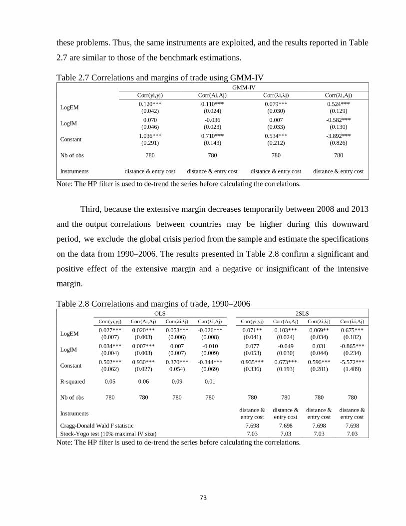
73
these problems. Thus, the same instruments are exploited, and the results reported in Table
2.7 are similar to those of the benchmark estimations.
Table 2.7 Correlations and margins of trade using GMM-IV GMM-IV
Corr(yi,yj) Corr(Ai,Aj) Corr(λi,λj) Corr(λi,Aj)
LogEM 0.120*** (0.042)
0.110*** (0.024)
0.079*** (0.030)
0.524*** (0.129)
LogIM 0.070
(0.046) -0.036 (0.023)
0.007 (0.033)
-0.582*** (0.130)
Constant 1.036*** (0.291)
0.710*** (0.143)
0.534*** (0.212)
-3.892*** (0.826)
Nb of obs 780 780 780 780
Instruments distance & entry cost distance & entry cost distance & entry cost distance & entry cost
Note: The HP filter is used to de-trend the series before calculating the correlations.
Third, because the extensive margin decreases temporarily between 2008 and 2013
and the output correlations between countries may be higher during this downward
period, we exclude the global crisis period from the sample and estimate the specifications
on the data from 1990–2006. The results presented in Table 2.8 confirm a significant and
positive effect of the extensive margin and a negative or insignificant of the intensive
margin.
Table 2.8 Correlations and margins of trade, 1990–2006 OLS 2SLS
Corr(yi,yj) Corr(Ai,Aj) Corr(λi,λj) Corr(λi,Aj) Corr(yi,yj) Corr(Ai,Aj) Corr(λi,λj) Corr(λi,Aj)
LogEM 0.027*** (0.007)
0.020*** (0.003)
0.053*** (0.006)
-0.026*** (0.008)
0.071** (0.041)
0.103*** (0.024)
0.069** (0.034)
0.675*** (0.182)
LogIM 0.034*** (0.004)
0.007*** (0.003)
0.007 (0.007)
-0.010 (0.009)
0.077
(0.053) -0.049 (0.030)
0.031 (0.044)
-0.865*** (0.234)
Constant 0.502*** (0.062)
0.930*** (0.027)
0.370*** 0.054)
-0.344*** (0.069)
0.935*** (0.336)
0.673*** (0.193)
0.596*** (0.281)
-5.572*** (1.489)
R-squared 0.05 0.06 0.09 0.01
Nb of obs 780 780 780 780 780 780 780 780
Instruments distance & entry cost
distance & entry cost
distance & entry cost
distance & entry cost
Cragg-Donald Wald F statistic 7.698 7.698 7.698 7.698
Stock-Yogo test (10% maximal IV size) 7.03 7.03 7.03 7.03
Note: The HP filter is used to de-trend the series before calculating the correlations.

74
Table 2.9 Correlations and margins of trade in capital goods OLS 2SLS
Corr(yi,yj) Corr(Ai,Aj) Corr(λi,λj) Corr(λi,Aj) Corr(yi,yj) Corr(Ai,Aj) Corr(λi,λj) Corr(λi,Aj)
LogEM 0.035*** (0.007)
0.021*** (0.004)
0.018*** (0.007)
0.004 (0.008)
0.101** (0.048)
0.111*** (0.030)
0.074*** (0.038)
0.612*** (0.131)
LogIM 0.036*** (0.006)
0.012*** (0.003)
0.017*** (0.005)
-0.03*** (0.006)
0.070*** (0.028)
-0.010 (0.017)
0.017 (0.022)
-0.349*** (0.076)
Constant 0.618*** (0.050)
0.928*** (0.028)
0.512*** (0.041)
-0.051*** (0.052)
1.03*** (0.197)
0.856*** (0.123)
0.590*** (0.154)
-2.592*** (0.536)
R-squared 0,13 0.09 0.05 0.03
Nb of obs 780 780 780 780 780 780 780 780
Instruments distance & entry cost
distance & entry cost
distance &entry cost
distance & entry cost
Cragg-Donald Wald F statistic 12.28 12.28 12.28 12.28
Stock-Yogo test (10% maximal IV size) 7.03 7.03 7.03 7.03
Note: The HP filter is used to de-trend the series before calculating the correlations.
Fourth, we decompose the bilateral trade intensity into trade in capital goods,
intermediate goods and consumptions goods. The effects of trade margins of these types of
goods on business cycle comovement are reported in Tables 2.9–2.11. We find that the
effects are similar to those of the baseline estimations in the cases of capital goods and
consumption goods. However, the instruments are weak in the case of intermediate goods.
Trade in intermediate goods involves vertical trade (importing intermediates for re-
exporting as intermediates) and processing trade (importing intermediates for re-exporting
as final goods). As such, entry cost is may not be strong enough to account for this feature
of the extensive margin of trade in intermediate goods. Thus, we use a country pair dummy
variable that equals one if both countries are developed and zero otherwise since different
stages in production process may be allocated based on the country’s level development.
Moreover, the level of country development may affect the capacity to generate new
products via technological innovation. The estimated results are reported in Table 2.12. The
hypothesis that instruments are weak is rejected. In fact, we find positive and significant
effects of the extensive margin of trade on business cycle comovement and its determinants.
Finally, we re-estimate the specifications when the extensive and intensive margins
are measured using only exports. This means that we calculate these two explicative
variables using only export data from country i to country j and EMij and IMij. The results
reported in Table 2.13 do not differ from the benchmark estimation.
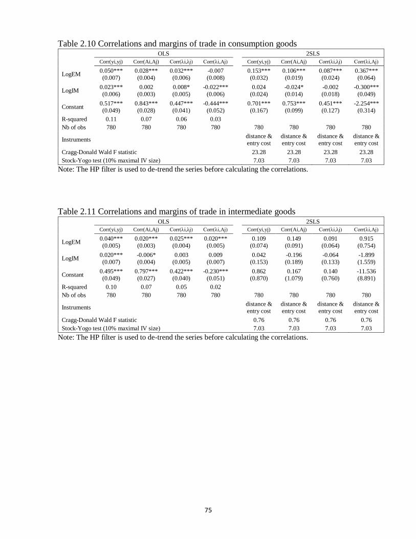
75
Table 2.10 Correlations and margins of trade in consumption goods OLS 2SLS
Corr(yi,yj) Corr(Ai,Aj) Corr(λi,λj) Corr(λi,Aj) Corr(yi,yj) Corr(Ai,Aj) Corr(λi,λj) Corr(λi,Aj)
LogEM 0.050*** (0.007)
0.028*** (0.004)
0.032*** (0.006)
-0.007 (0.008)
0.153*** (0.032)
0.106*** (0.019)
0.087*** (0.024)
0.367*** (0.064)
LogIM 0.023*** (0.006)
0.002 (0.003)
0.008* (0.005)
-0.022*** (0.006)
0.024
(0.024) -0.024* (0.014)
-0.002 (0.018)
-0.300*** (0.049)
Constant 0.517*** (0.049)
0.843*** (0.028)
0.447*** (0.041)
-0.444*** (0.052)
0.701*** (0.167)
0.753*** (0.099)
0.451*** (0.127)
-2.254*** (0.314)
R-squared 0.11 0.07 0.06 0.03
Nb of obs 780 780 780 780 780 780 780 780
Instruments distance & entry cost
distance & entry cost
distance & entry cost
distance & entry cost
Cragg-Donald Wald F statistic 23.28 23.28 23.28 23.28
Stock-Yogo test (10% maximal IV size) 7.03 7.03 7.03 7.03
Note: The HP filter is used to de-trend the series before calculating the correlations.
Table 2.11 Correlations and margins of trade in intermediate goods OLS 2SLS
Corr(yi,yj) Corr(Ai,Aj) Corr(λi,λj) Corr(λi,Aj) Corr(yi,yj) Corr(Ai,Aj) Corr(λi,λj) Corr(λi,Aj)
LogEM 0.040*** (0.005)
0.020*** (0.003)
0.025*** (0.004)
0.020*** (0.005)
0.109
(0.074) 0.149
(0.091) 0.091
(0.064) 0.915
(0.754)
LogIM 0.020*** (0.007)
-0.006* (0.004)
0.003 (0.005)
0.009 (0.007)
0.042
(0.153) -0.196 (0.189)
-0.064 (0.133)
-1.899 (1.559)
Constant 0.495*** (0.049)
0.797*** (0.027)
0.422*** (0.040)
-0.230*** (0.051)
0.862
(0.870) 0.167
(1.079) 0.140
(0.760) -11.536 (8.891)
R-squared 0.10 0.07 0.05 0.02
Nb of obs 780 780 780 780 780 780 780 780
Instruments distance & entry cost
distance & entry cost
distance & entry cost
distance & entry cost
Cragg-Donald Wald F statistic 0.76 0.76 0.76 0.76
Stock-Yogo test (10% maximal IV size) 7.03 7.03 7.03 7.03
Note: The HP filter is used to de-trend the series before calculating the correlations.

76
Table 2.12 Correlations and margins of trade in intermediate goods with dummy instrument
variable OLS 2SLS
Corr(yi,yj) Corr(Ai,Aj) Corr(λi,λj) Corr(λi,Aj) Corr(yi,yj) Corr(Ai,Aj) Corr(λi,λj) Corr(λi,Aj)
LogEM 0.040*** (0.005)
0.020*** (0.003)
0.025*** (0.004)
0.020*** (0.005)
0.191*** (0.023)
0.120*** (0.016)
0.133*** (0.019)
-0.025 (0.017)
LogIM 0.020*** (0.007)
-0.006* (0.004)
0.003 (0.005)
0.009 (0.007)
-0.117***
(0.050) -0.139***
(0.034) -0.147***
(0.042) -0.075***
(0.035)
Constant 0.495*** (0.049)
0.797*** (0.027)
0.422*** (0.040)
-0.230*** (0.051)
-0.025 (0.306)
0.148 (0.211)
-0.324 (0.255)
-0.850*** (0.210)
R-squared 0.10 0.07 0.05 0.02
Nb of obs 780 780 780 780 780 780 780 780
Instruments distance &
dummy distance &
dummy distance &
dummy distance &
dummy
Cragg-Donald Wald F statistic 16.47 16.47 16.47 16.47
Stock-Yogo test (10% maximal IV size) 7.03 7.03 7.03 7.03
Note: The HP filter is used to de-trend the series before calculating the correlations.
Table 2.13 Extensive and intensive margin measured only using exports OLS 2SLS
Corr(yi,yj) Corr(Ai,Aj) Corr(λi,λj) Corr(λi,Aj) Corr(yi,yj) Corr(Ai,Aj) Corr(λi,λj) Corr(λi,Aj)
LogEM 0.097*** (0.013)
0.052*** (0.007)
0.055*** (0.011)
-0.031** (0.014)
0.347*** (0.050)
0.199*** (0.029)
0.181*** (0.037)
0.469*** (0.123)
LogIM 0.012
(0.009) -0.002 (0.005)
0.002 (0.007)
0.024** (0.009)
0.026
(0.062) -0.069** (0.036)
-0.019 (0.045)
-0.713*** (0.151)
Constant 0.380*** (0.038)
0.825*** (0.021)
0.384*** (0.031)
-0.363*** (0.039)
0.680*** (0.216)
0.700*** (0.124)
0.424*** (0.156)
-2.646*** (0.524)
R-squared 0.07 0.06 0.04 0.02
Nb of obs 780 780 780 780 780 780 780 780
Instruments distance & entry cost
distance & entry cost
distance & entry cost
distance & entry cost
Cragg-Donald Wald F statistic 12.44 12.44 12.44 12.44
Stock-Yogo test (10% maximal IV size) 7.03 7.03 7.03 7.03
Note: The HP filter is used to de-trend the series before calculating the correlations.

77
2.5. Conclusion
Theoretical models are unable to fully replicate the relation between business cycle
comovement and trade observed from the data. Kose and Yi (2006) have termed this
phenomenon the trade-comovement puzzle. To solve this puzzle, Juvenal and Santos-
Monteiro (2017) have proved that the output correlation should be explained by three
component factors: correlation between each country's TFP, correlation between each
country's share of expenditure on domestic goods, and correlation between each
country’s TFP and the trading partner’s share of expenditure on domestic goods. They have
illustrated that most models generate a counterfactual relation between trade and the
comovement of share of expenditure on domestic goods. In this chapter, we have
empirically investigated the effect of extensive margin of trade on business cycle
comovement and its determinants. First, we have re-examined the business comovement
factor structure, determining that the first two component factors drive the business cycle
synchronization. On the other hand, the effect of the third factor is not significant. By
decomposing bilateral trade into extensive and intensive margins, we have observed that
the extensive margin of trade not only synchronizes TFP shocks through transmitting new
technology embedded in varieties of goods (Liao and Santacreu, 2015) but also favors the
correlation between each country's share of expenditure on domestic goods. In fact, the
effect of the intensive margin is negative or not significant. Thus, we suggest that
theoretical models should allow for extensive margin of trade in order to solve the puzzle.
In such models, following a productivity shock in the Home country, the productivity
threshold for firms to export falls. This fall raises the number of domestic firms and number
of new products in the tradable sector. The prices of domestic exported products do not
change, even increase. The correlation of aggregate productivities and shares of expenditure
in domestic goods increase with trade in varieties. These higher correlations induces an
increase in business cycle comovement. Since the extensive margin of trade, and not the
intensive margin, enhances comovement, countries should encourage the trade of new
products in order to increase synchronization.

78
The existing literature on the trade-comovement puzzle has only focused on the
unanticipated productivity shock. However, recent empirical evidence has noted important
differences between the transmission of unanticipated (surprise) TFP shock and anticipated
(news) TFP shock. For instance, Levchenko and Pandalai-Nayar (2018) have suggested
that while the news TFP shocks occurring in the US generate Canadian business cycle in
the medium term, US surprise TFP shocks have no effect on the neighboring economy.
Nam and Wang (2015) have emphasized the important role of news TFP shock in
comparison with the traditional surprise TFP shock on the transmission via trade channels.
Thus, the trade-comovement puzzle may originate from this source of macro aggregate
fluctuations. The next and final chapter adds to the literature by identifying evidence for
the transmission of news TFP shock via trade channel. More specifically, the contribution
brings a new viewpoint on one of the sources of the international business cycle: news TFP
shock.
79
References
Arkolakis, C., Ramanarayanan, A., 2009. Vertical specialization and international business
cycle synchronization. Scandinavian Journal of Economics. 111 (4), 655–680.
Baxter, M., Kouparitsas, M., 2005. Determinants of business cycle comovement: a robust
analysis. Journal of Monetary Economics. 52 (1), 113–157.
Clark, T., Van Wincoop, E., 2001. Borders and business cycles. Journal of International
Economics 55 (1), 59–85.
Di Giovanni, J., Levchenko, A.A., 2010. Putting the parts together: trade, vertical linkages,
and business cycle comovement. American Economic Journal: Macroeconomics, 2 (2),
95–124.
Djankov, S., La Porta, R., Lopez-De Silanes, F., Shleifer, A., 2002. The regulation of entry,
Quarterly Journal of Economics. 117 (1), 1.
Drozd, L., Kolbin S., and Nosal, J., 2017. Long-Run Price Elasticity of Trade and the Trade-
Comovement, 2017 Meeting Papers 204, Society for Economic Dynamics.
Dutt, P., Mihov, I. and Van Zandt, T., 2013. The effect of WTO on the extensive and the
intensive margins of trade. Journal of International Economics, pages 204-219.
Frankel, J., Rose, A., 1998. The endogeneity of the optimum currency area criteria.
Economic Journal. 108 (449), 1009–1025.
Gaulier, G., Zignago, S., 2010. BACI: International Trade Database at the Product-Level.
The 1994-2007 Version. CEPII Working Paper 2010- 23.
Gujarati, D. 2003. Basic Econometrics, 4th Edition. New York, NY: McGraw Hill Inc.
Hummels, D., Klenow, P., 2005. The variety and quality of a nation's exports. American
Economic Review. Rev. 704–723.
Imbs J., 2004, Trade, Finance, Specialization and Synchronization. The Review of
Economics and Statistics, MIT Press, vol. 86(3), pages 723-734, August.
Johnson, R.C., 2014. Trade in intermediate inputs and business cycle comovement.
American Economic Journal: Macroeconomics. 6 (4), 39–83.

80
Juvenal, L., Santos Monteiro, P., 2017. Trade and synchronization in a multi-country
economy. European Economic Review, 97, 385-415.
Kose, M.A., Yi, K.-M., 2006. Can the standard international business cycle model explain
the relation between trade and comovement? Journal of International Economics. 68,
267– 295.
Liao W., and Santacreu A. M., 2015. The trade-comovement puzzle and the margins of
international trade. Journal of International Economics, Volume 96, Issue 2, Pages 266-
288, ISSN 0022-1996.
Naknoi, 2015. Exchange rate volatility and fluctuations in the extensive margin of trade,
Journal of Economic Dynamics & Control
http://dx.doi.org/10.1016/j.jedc.2014.12.007.
Ng, E., 2010. Production fragmentation and business cycle comovement. Journal of
International Economics. 82(1), 1–14.
Pentecôte J.-S., J.-C. Poutineau and Rondeau F., 2015. Trade Integration and Business
Cycle Synchronization in the EMU: the Negative Effect of New Trade Flows. Open
Economies Review, vol. 26(1).
Wong C.-Y., and Eng Y.-K., 2013. International business cycle co-movement and vertical
specialization reconsidered in multistage Bayesian DSGE model. International Review
of Economics & Finance, Volume 26, Pages 109-124, ISSN 1059-0560.
Zlate A., 2016. Offshore production and business cycle dynamics with heterogeneous firms.
Journal of International Economics, Volume 100, Pages 34-49, ISSN 0022-1996.

81
Appendix
Table 2.A.1 Descriptive Statistics
Variable Nb. of Obs. Mean Std. Dev. Min Max
Corr(yi,yj) 780 0.23 0.32 -0.71 0.90
Corr(Ai,Aj) 780 0.78 0.18 0.00 0.99
Corr(λi,λj) 780 0.32 0.27 -0.63 0.89
Corr(λi,Aj) 780 -0.23 0.32 -1.17 0.63
EMij 780 0.280 0.250 0.000 0.960
IMij 780 0.002 0.016 0.000 0.375
Trade1ij 780 0.012 0.025 0.000 0.293
Trade2ij 780 0.006 0.020 0.000 0.315

82
Table 2.A.2 Our results versus Liao and Santacreu (2015) and Juvenal and Santos-Monteiro (2017)
OLS 2SLS J&SM2017 L&S2015
Corr(yi,yj) Corr(yi,yj) Corr(Ai,Aj) Corr(λi,λj) Corr(yi,yj) Corr(yi,yj) Corr(Ai,Aj) Corr(λi,λj) Corr(yi,yj) Corr(Ai,Aj)
(1) (2) (3) (4) (5) (6) (7) (8) (9) (10)
Corr(Ai,Aj) 0.741***
(0.061)
0.135*
(0.069)
Corr(λi,λj) 0.207***
(0.043)
0.320***
(0.062)
Corr(Ai,λj) -0.019
(0.032)
-0.282*
( 0.153)
Log(Tradeij) 0.103***
(0.021)
0.061***
(0.021)
0.074***
(0.023)
Log(EMij)
0.120***
(0.041)
0.110***
(0.026)
0.079**
(0.032)
0.155***
(0.029)
0.138***
(0.025)
Log(IMij) 0.070
(0.045)
-0.036
(0.029)
0.007
(0.035)
0.016
(0.014)
-0.021
(0.012)
Constant -0.421***
(0.046)
1.036***
(0.292)
0.710***
(0.186)
0.534**
(0.227)
0.266***
(0.047)
0.963***
(0.093)
0.560***
(0.100)
0.937***
(0.099)
0.644***
(0.080)
0.215**
(0.071)
R-squared 0.24 0.17 0.1 0.03 0.04
Nb. of obs. 780 780 780 780 210 210 210 210 2610 2610
Instruments distance &
entry-cost
distance &
entry-cost
distance &
entry-cost
distance &
entry-cost
distance &
entry cost
Cragg-Donald
Wald 8.381 8.381 8.381
Stock-Yogo
10% 7.03 7.03 7.03
Notes: Numbers in parentheses are standard errors; ***, **, * significant at 1%, 5% and 10%, respectively. HP filter is used to detrend the raw series. This Appendix resumes our estimated results and that of Liao and Santacreu (2015) and Juvenal and Santos-Monteiro (2017). Column (1) shows our
updated factor structure of business cycle comovement. Columns (2) and (3) show effects of the margins of trade on output and TFP comovements.
These results are in line with two studies, which is reported in columns 5, 6, 7, 9 and 10. Column (4) shows our main contribution. The coefficient
of the extensive margin is significant at 5% confidence level and equals to 0.079 (compared to 0.074 of the effect of total trade in Juvenal and Santos-Monteiro, 2017, reported in column 8). The intensive margin has no significant effect. This finding emphasizes that the extensive margin is mainly
responsible for the empirical positive effect of trade on the comovement of share of expenditure on domestic goods.
83
CHAPTER 3
NEWS TFP SHOCK, TRADE AND BUSINESS CYCLE
TRANSMISSION TO SMALL OPEN ECONOMIES
Highlights
The trade-comovement puzzle may arise from sources of aggregate fluctuations.
Theoretical models (Kose and Yi, 2006, Liao and Santacreu, 2015, Juvenal and Santos-
Monteiro, 2017, among others) have focused on the surprise Total Factor Productivity
(TFP) shock. In their models, a positive surprise TFP shock generates an increase in
domestic demand. This fluctuation is then transmitted to foreign economies via the
demand-supply channel of trade. However, recent empirical evidence (Levchenko and
Pandalai-Nayar, 2018) has suggested that news TFP shock, and not surprise TFP shock, is
responsible for the economic cycle transmission. This chapter provides more empirical
evidence regarding the demand-supply mechanism of trade through investigating the
cross-border transmission of news TFP shocks and thereby contributing to understanding
the puzzle. We use a structural VAR model to investigate the responses of trade and macro
aggregates in four advanced economies, Australia, Canada, New Zealand and the United
Kingdom, to a news TFP shock occurring in the United States. The news shocks are
identified as in Barsky and Sims (2011). By running the model on data over the post-
Bretton Woods period (1973Q1- 2016Q4), we obtain two findings. First, real exchange
rate, terms-of-trade and bilateral trade between these economies and the United States
reacts to news TFP shocks in a different way than contemporaneous TFP shocks. These
results are in line with those of Nam and Wang (2015). Second, the business cycles of
these economies are affected by news rather than contemporaneous TFP shocks in the
United States. News TFP shocks are therefore an important source of the international

84
business cycle instead of contemporaneous TFP shocks, a proposition which has been well
documented in the literature.
JEL classification: E32, F4, F41
Keywords: News-driven business cycle, News TFP shock, Business cycle transmission,
Small open economy

85
3.1. Introduction and Literature Review
News TFP shocks (or anticipated TFP shocks) are shocks that have no immediate impact
on productivity, but portend its movements in the near future. Discoveries, inventions, and
technological innovations need time to enhance productivity. For example, Internet of
Things technologies, 3D printing technology, self-driving cars, hyperloop train, and smart
robots have not yet become popular, although we have known about them for a long time.
Otherwise, contemporaneous TFP shocks (or surprise TFP shocks, unanticipated TFP
shocks) are shocks that immediately affect productivity. Given the rapid development of
information and communication technology over the last two decades, most productivity
shocks are news shocks. In fact, recent empirical evidence has suggested that news TFP
shocks generate business cycles (Barsky and Sims, 2011, Beaudry et al., 2011b, Fujiwara
et al., 2011, Nam and Wang, 2015, Kamber et al., 2017, among others). In a globalizing
world, when a shock causes domestic macro fluctuations, the question of transmission
across countries is important. Yet, whereas transmission mechanisms of surprise TFP
shocks in open economies have attracted the attention of many researchers, there is limited
empirical evidence regarding news TFP shock transmission across countries. Therefore,
this chapter focuses on the cross-border transmission of news TFP shocks. We empirically
investigate its role on trade behavior and international business cycle convergence.
Most theoretical models have focused on the effects of news shocks on real activity.
They have not addressed the transmission of this type of shock via trade channel. The first
work on modeling the role of news shock in explaining business cycles is that of Beaudry
and Portier (2004). In their research, the authors constructed a general equilibrium structure
model to formalize the idea that difficulties encountered by forward-looking agents in
forecasting the economy may induce booms and recessions. This view has had a long
history since it was first elaborated by Pigou (1927). However, there has been a growing
interest in explaining business cycles by the news about future total factor productivity.
Fujiwara et al. (2011) have investigated whether news TFP shock can be a major source of
aggregate fluctuations. They have extended a DSGE model by allowing news TFP shocks

86
and estimating for the United States and Japan using Bayesian methods. Their three results
are that news TFP play a more important role in the US than in Japan, the effects of news
shock are more important with longer forecast horizon, and news TFP shocks make the
overall effect of productivity on hours worked ambiguous. Schmitt-Grohé and Uribe (2012)
have estimated, in the context of a DSGE model, the contributions of anticipated shocks to
the post-war US business cycles by using classical maximum likelihood and Bayesian
methods. They have considered several structural shocks, including shock to productivity,
shock to government spending, shock to wage markup, and preference shocks. Each of
these shocks consists of a news component and a surprise component. For the anticipated
component, they have distinguished the anticipation horizons, which means that positive
(or negative) news may be repeated several times before realization. Their findings have
suggested that approximately half of predicted aggregate movements in output,
consumption, investment, and employment are explained by anticipated shocks. Beaudry
et al. (2011) have developed a model to simulate the way news shocks generate positive
co-movements in real activity across countries. They have indicated that news TFP shocks
provide a driving force of business cycles synchronization.
On the empirical front, most studies based on news TFP shock identification
schemes have been proposed by Beaudry and Portier (2006) and Barsky and Sims (2011).
These studies have pointed out that news TFP shocks account for a significant fraction of
macroeconomic aggregates fluctuations. Beaudry and Portier (2006) have noted that news
TFP shocks account for nearly half of business cycle fluctuations. These news shocks
generate a boom in consumption, investment, and hours worked. These results are obtained
from a news shock identification scheme in which the effect of news TFP shock is imposed
as zero over the first periods. In contrast, Barsky and Sims (2011) have proposed a news
TFP shock identification approach using a structural VAR framework, in which news TFP
shocks are imposed to have no impact on current factors-utilization-adjusted TFP and are
orthogonal to the surprise shock. They have suggested that movements in factors-
utilization-adjusted TFP are fully explained by these two shocks. After running the model

87
on the US’s data from 1960 to 2007, the authors found that positive news about future
productivity declines output, investment and employment but increases consumption.
However, studying news TFP shocks is insufficient to understand recessions. Beaudry et
al. (2013) have indicated that the two identification approaches drive similar results. Some
empirical studies have addressed the transmission of news TFP shock via the trade channel.
For instance, empirical evidence for the US economy, as concluded by Nam and Wang
(2015), has suggested that there are distinct dynamics for bilateral trade variables (net trade,
real exports, and real imports) following surprise and anticipated shocks to productivity.
The responses of international relative prices (real exchange rate and terms-of-trade) are
also different. In particular, whereas good news about future productivity appreciates terms-
of-trade and real exchange rate, surprise shock depreciates them. The authors therefore have
concluded that ignoring news components in TFP shock may induce misleading
conclusions.
More specifically, two studies relate directly to our work. Levchenko and Pandalai-
Nayar (2018) have recently used a SVAR model to estimate the international transmission
of three types of shock, news TFP shock, surprise TFP shock and “sentiment” (non-
technology) shock. They have found that for the US-Canada country pair, news TFP shock
is a source of co-movement in the medium- and long-term, whereas surprise TFP
innovations do not generate synchronization. In the short-term, “sentiment” shock
dominates the surprise and news TFP shock in producing business cycle co-movement
between the US and Canada. They have focused on the transmission of sentiment shock
exclusively for the US-Canada. Given that news TFP shock may be a solution for the trade-
comovement puzzle, this chapter focuses exclusively on the transmission of this type of
shock. Our work is thus distinguished from their paper since we focus on the transmission
of news TFP shocks to other small open countries via the trade channel. Moreover, as TFP
shocks influence relative prices, we investigate the responses of the volume of trade (export
and import) as well as the international prices (real exchange rate and the terms-of-trade)
to news and surprise TFP shocks as in Nam and Wang (2015).

88
Kamber et al. (2017) have focused on the responses of aggregate macroeconomic
variables in four advanced small open economies, Australia, Canada, New Zealand and the
United Kingdom, following a news shock in domestic TFP (since these four economies are
relatively small in terms of GDP size with respect to the US GDP, they call them advanced
small open countries). By estimating four country-specific VAR models, they have
discovered that expected shocks to productivity generate comovement between real output,
employment, consumption and investment. Good news about future productivity in a given
country also induces a decrease in its net trade. These authors have highlighted that news
TFP shocks are related to the comovement between aggregate variables as well as
countercyclical current account dynamics. In this chapter, we reexamine these four
advanced open economies (Australia, Canada, New Zealand and United Kingdom).
However, our work differs from their study as we investigate the impact of foreign news
TFP shocks on these economies. In other words, while we study the transmission of news
TFP shocks, they focus on impact of domestic news TFP shocks.
By studying the responses of macro aggregates and bilateral trade in four advanced
small open economies following news and surprise TFP shocks experienced in the United
States, this chapter examines the role of news TFP shock on the international business cycle
convergence. Advanced small open economies are used as a case study to analyze these
issues due to their small sizes relative to the US, which renders them more sensible to the
shock. Moreover, macro fluctuations in these countries do not affect US TFP shocks. As
such, we obtain two findings. First, the effects of news TFP shocks on real exchange rate,
terms-of-trade and bilateral export and import between small open economies and the
United States are different from that of contemporaneous TFP shocks. News TFP shocks
in the US favor its import from small trading partners while surprise TFP shocks do not.
The increase in US domestic demand is thereby transmitted to foreign economies through
demand-supply mechanism of trade. This fact is demonstrated in the second finding: the
business cycles of the small open economies are significantly affected by the economic
booms in the United States generated by news TFP shocks. The TFP news shocks are thus
89
an important source of the international business cycle and should be considered in a
theoretical model in order to replicate the trade-comovement relationship.
The rest of the chapter is organized as follows: Section 2 presents the empirical
strategy, section 3 describes the data and stylized facts, section 4 discusses the main
empirical results and section 5 offers a conclusion.
3.2. Empirical Strategy
3.2.1 SVAR Model and Estimation Strategy
To study the responses of macroeconomic aggregates as well as bilateral trade variables
(both quantity and price effects) of open small economies when news TFP shocks occur in
their trading partner, we use a SVAR model in which news shocks about the future of total
factor productivity are identified as in Barsky and Sims (2011).
We follow Levchenko and Pandalai-Nayar (2018) to choose the estimation strategy.
First, we estimate a reduced form VAR in order to evaluate the responses of the US
economy when facing news and surprise TFP shocks:
tt
p
ptt uYLCLYCCY ...10
where Yt is the matrix of variables as described below, C refers to matrix of parameters to
be estimated, L is lag operators and ut denotes matrix of residuals.
This model highlights the differences in impulse responses of the US
macroeconomic aggregates to surprise and news TFP shocks. It is an extension of the five-
variable VAR model estimated in Barsky and Sims (2011). The variables include:
Utilization-adjusted TFP of the US, US Real GDP, US real investment (private non-
residential gross fixed capital formation as proxy - INV), US real consumption (CON), US
employment equal to worked hours multiplied by number of persons (EMP). We also add
the variable share of expenditure on domestic goods of the United States (SHARE, equal
to one minus the import penetration ratio) to determine how consumption structure changes
when facing TFP news and surprise shocks. This variable helps forecast the behavior of
90
exports and imports with trading partners. We call this six-variable model the “core VAR”
model.
To estimate the cross-border transmission of news and surprise TFP shocks in the
US to other countries, we follow Levchenko and Pandalai-Nayar (2018) in estimation
strategy. We include variables of small open countries one by one and order it last in a
seven-variable VAR model (“core VAR” model + 1 variable) as macro fluctuations in
advanced small economies do not influence the US macro aggregates. The eight variables
considered for small open economies are: Real export from each country to the United
States (EXP), real import to each country from the United States (IMP), real GDP of each
country, real investment of each country (INV, private non-residential gross fixed capital
formation is taken as proxy), real consumption of each country (CON), employment equal
worked hours multiplied by number of persons (EMP), real exchange rate of the US dollar
and each small open country’s currency (RER), and relative terms-of-trade between the
United States and each small open country (TOT). We follow Nam and Wang (2015) by
calculating TOT and RER and including them in the model. First, the real exchange rate
between country H and country F is calculated as the ratio between the CPI of country H in
country F’s currency to CPI of country F. It is equal to:
RER =CPIH in H′s currency × Nominal exchange rate H/F
CPIF in F′s currency
As a result, increases in the real exchange rate mean that the currency of country H
appreciates versus the currency F. Second, and similarly, the terms-of-trade is measured by
using the nominal exchange rate and the export deflators. It equals to:
TOT =Export DeflatorH in H′s currency × Nominal exchange rate H/F
Export DeflatorF in F′s currency

91
The terms-of-trade represents the international relative price of traded goods. An increase
in the measure of terms-of-trade indicates that the traded goods of country H are more
expensive relative to those of country F. In this study, country H is the United States and F
is a considered an open country.
Hence, for each of the four small open economies, we run the seven-variable SVAR
model eight times to have impulse responses of macroeconomic variables as well as trade
and relative prices to a favorable news TFP shock in the United States. The same exercise
is realized in the case of the surprise shock.
The lag9 of the model is chosen to be three. As suggested by Barsky and Sims (2011),
all variables added in the system are in level. Barsky and Sims (2011) have proposed that
estimating the VAR system in levels produces consistence estimates of impulse responses.
It is also sufficiently robust to the cointegration of unknown form. According to these
authors, although estimating the model in levels or differences produces similar results, the
level specification is preferred as the invalid assumptions concerning the common trend
can yield misleading conclusions.
3.2.2 News TFP Shock Identification Scheme
We identify the news shock in the SVAR model by using the identification scheme
developed by Barsky and Sims (2011). This identification method is described below.
Assuming that TFP follows a process:
LnAt = [B11(L) B12(L) ] [ε1,t
ε2,t] (3.1)
where At denotes the TFP at year t, ε1,t is the surprise technology shock and ε2,t is the news
shock. Barsky and Sims (2011) have only imposed the restriction B12(0) = 0, so that news
shock does not immediately affect technology. The TFP at a given point in time is affected
by three factors, contemporaneous shock, past news shocks, and past TFP changes:
9 We follow Levchenko and Pandalai-Nayar (2018) to choose lag based on the Akaike Information Criterion.
92
LnAt = LnAt−1 + ε1,t + ε2,t−j (3.2)
They have identified the unanticipated (surprise) shock as the reduced form
innovation in TFP. The anticipated (news) shock is then identified as the shock that best
explains the remaining TFP future movements. In other words, the news TFP shocks are
identified as the first principal component of observed TFP over all forecast horizons, up
to a truncation horizon.
Assuming we have a VAR model of observables yt:
tt uLBy )(
with a linear mapping between innovations and structural shocks:
tt Au 0
The model is then re-written:
tot LCy )(
where 0)()( ALBLCo and tt uA 1
0
.
The h step ahead forecast error is:
h
t
hthttht DByEy0
01 Ã
where Ã0D is the entire space of permissible impact matrices with D a orthogonal matrix.
The share of the forecast error variance that structural shock j contributes to variable i at
horizon h is then:
h
ii
h
ii
h
ii
i
h
jji
ji
BB
BB
eBBe
eBDeDeBe
h
0
'
,,
0
'
,
'
00,
0
''
0
''
0
'
0
'
,
Ã'Ã
)(
)Ã'Ã(
)(
where ei is the selection vector in which ith element equals to 1 and the others equal to 0.
Equations (3.1) and (3.2) imply that surprise and news shock account for all variations in
TFP at all horizons. In the case that TFP occupies the first position in the system, the
surprise shock is indexed by 1, the news shock is indexed by 2, and we have:
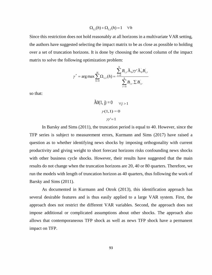
93
1)()( 2,11,1 hh h
Since this restriction does not hold reasonably at all horizons in a multivariate VAR setting,
the authors have suggested selecting the impact matrix to be as close as possible to holding
over a set of truncation horizons. It is done by choosing the second column of the impact
matrix to solve the following optimization problem:
H
hh
ii
h
ii
BB
BB
h0
0
'
,,
0
'
,
'
00,
2,1
*
Ã'Ã
)(maxarg
so that:
0 = j)Ã0(1, 1j
0 = (1,1)
1'
In Barsky and Sims (2011), the truncation period is equal to 40. However, since the
TFP series is subject to measurement errors, Kurmann and Sims (2017) have raised a
question as to whether identifying news shocks by imposing orthogonality with current
productivity and giving weight to short forecast horizons risks confounding news shocks
with other business cycle shocks. However, their results have suggested that the main
results do not change when the truncation horizons are 20, 40 or 80 quarters. Therefore, we
run the models with length of truncation horizon as 40 quarters, thus following the work of
Barsky and Sims (2011).
As documented in Kurmann and Otrok (2013), this identification approach has
several desirable features and is thus easily applied to a large VAR system. First, the
approach does not restrict the different VAR variables. Second, the approach does not
impose additional or complicated assumptions about other shocks. The approach also
allows that contemporaneous TFP shock as well as news TFP shock have a permanent
impact on TFP.

94
3.3. Data and Stylized Facts
Data is extracted over the post-Bretton Woods period: 1973Q1–2016Q4. In the news shock
identification approach discussed above, Barsky and Sims (2011) have imposed the
restriction that news TFP shock have no impact on current TFP. As the factor utilization –
or the intensity that capital and labor are used – responds immediately when a news TFP
shock occurs (see Jaimovich and Rebelo, 2009, and Nam and Wang, 2010), this restriction
is no longer valid if data on TFP are not adjusted for input utilization. In addition, Barsky
and Sims (2011) have supposed that all movements in the true TFP are fully explained by
contemporaneous and news shocks, the non-adjusted TFP series may be driven by
unobserved factors. Therefore, the TFP series must be adjusted for the utilization rate.
Fernald (2014) has produced a quarterly measure for the United States of utilization-
adjusted TFP by relying on the annual estimates for utilization from Basu et al. (2006). We
have obtained these data from Fernald’s website, wherein the author has posted the series
in terms of annualized percentage changes. We have divided the original series by 400 and
then cumulated them to recover the quarterly TFP series in levels. The first point of
productivity series is assumed to be 1. The recovered series is illustrated in Figure 3.1,
indicating an increasing trend of the US productivity from 1973Q1 to 2016Q4.

95
Figure 3.1 US utilization-adjusted Total Factor Productivity (1973Q1–2017Q3)
Source: Fernald’s website.
Output, consumption, and investment (in constant local currency) data are extracted
from the OECD Economic Outlook database. Employment is calculated by multiplying the
total hours worked by the number of working persons. These series are available in the
OECD database. All macroeconomic aggregates are taken as logarithms before running the
estimation. Bilateral trade in current US dollars comes from the Direction of Trade
Statistics (DOTS) database of the IMF. These series are then deflated by the GDP deflator,
which has been taken from the International Financial Statistic (IFS) of the IMF. In order
to compute the share of expenditure in domestic goods of the United States, we obtain the
total exports and imports in current dollars from the OECD database. The nominal
exchange rate series are from IFS. Lastly, the CPI and export deflators are also taken from
the OECD Economic Outlook.
0.9
0.95
1
1.05
1.1
1.15
1.2
1.25
1.3
1.35
1973
:Q1
1974
:Q2
1975
:Q3
1976
:Q4
1978
:Q1
1979
:Q2
1980
:Q3
1981
:Q4
1983
:Q1
1984
:Q2
1985
:Q3
1986
:Q4
1988
:Q1
1989
:Q2
1990
:Q3
1991
:Q4
1993
:Q1
1994
:Q2
1995
:Q3
1996
:Q4
1998
:Q1
1999
:Q2
2000
:Q3
2001
:Q4
2003
:Q1
2004
:Q2
2005
:Q3
2006
:Q4
2008
:Q1
2009
:Q2
2010
:Q3
2011
:Q4
2013
:Q1
2014
:Q2
2015
:Q3
2016
:Q4
Utilization-adjusted TFP Non-adjusted TFP

96
Stylized facts
Table 3.1 Relative GDP size and Trade Intensity between four countries and the United
States (1973–2016)
Country %GDP/US TRI/US Rank of export to US Rank in import of US
Australia 5.55% 13.83% 4 24
Canada 9.40% 68.93% 1 1
New Zealand 0.90% 13.44% 2 36
United Kingdom 16.30% 11.35% 1 6 Notes: “%GDP/US” is the ratio between real GDP of each country and the US real GDP. “TRI/US” is the
trade intensity between each country and the US. “Rank of export to US” is the rank of the US market in
each country’s export markets. “Rank in import of US” represents the position of each considered country in a list of countries from which the US imports.
Table 3.1 presents information about the four advanced small open countries. The
second column indicates the GDP of these economies as a percentage of the US GDP, in
average, over the period 1973–2016. Compared to the US, these economies are relatively
small since their GDPs correspond to approximately 1% (New Zealand), 5.5% (Australia),
9.4% (Canada) and 16.3% (United Kingdom) of the US GDP. The third column represents
the trade intensity between each small economy and the US. This indicator is calculated as
the ratio of total bilateral trade with the US on its total trade:
itit
UStiUSti
iIMEX
IMEX
TUSTRI
__1/
where i is Australia, Canada, New Zealand or the United Kingdom. The numbers in the
third column, calculated by using quarterly data over 1973Q1–2016Q4, suggest that Canada
trades intensively with the US. The total exports and imports with the US account for nearly
70% of its total trade. Thus, the US is the largest export market of Canada, as indicated in
the fourth column (in average over 1973–2017). Trade intensities with the US are roughly
14%, 13.5% and 11% for the cases of Australia, New Zealand and United Kingdom,
respectively. The US is also the largest goods and services receiver of the UK, the third
largest export market of the New Zealand and the fourth largest export market in the case
of Australia (in average over 1973–2017). Column 4 reveals that the US imports mostly
from Canada. The United Kingdom occupies the sixth place in countries from which the
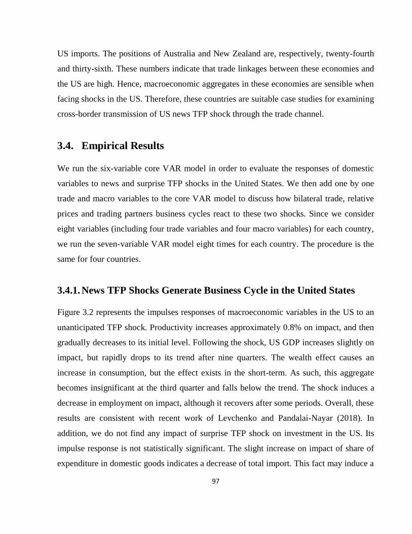
97
US imports. The positions of Australia and New Zealand are, respectively, twenty-fourth
and thirty-sixth. These numbers indicate that trade linkages between these economies and
the US are high. Hence, macroeconomic aggregates in these economies are sensible when
facing shocks in the US. Therefore, these countries are suitable case studies for examining
cross-border transmission of US news TFP shock through the trade channel.
3.4. Empirical Results
We run the six-variable core VAR model in order to evaluate the responses of domestic
variables to news and surprise TFP shocks in the United States. We then add one by one
trade and macro variables to the core VAR model to discuss how bilateral trade, relative
prices and trading partners business cycles react to these two shocks. Since we consider
eight variables (including four trade variables and four macro variables) for each country,
we run the seven-variable VAR model eight times for each country. The procedure is the
same for four countries.
3.4.1. News TFP Shocks Generate Business Cycle in the United States
Figure 3.2 represents the impulses responses of macroeconomic variables in the US to an
unanticipated TFP shock. Productivity increases approximately 0.8% on impact, and then
gradually decreases to its initial level. Following the shock, US GDP increases slightly on
impact, but rapidly drops to its trend after nine quarters. The wealth effect causes an
increase in consumption, but the effect exists in the short-term. As such, this aggregate
becomes insignificant at the third quarter and falls below the trend. The shock induces a
decrease in employment on impact, although it recovers after some periods. Overall, these
results are consistent with recent work of Levchenko and Pandalai-Nayar (2018). In
addition, we do not find any impact of surprise TFP shock on investment in the US. Its
impulse response is not statistically significant. The slight increase on impact of share of
expenditure in domestic goods indicates a decrease of total import. This fact may induce a

98
decline in export from trading partners to the US and is investigated in more detail in the
following sections. In sum, surprise TFP shocks only generate minute macro fluctuations
in the short-term in the US. Moreover, this shock does not cause comovement between
GDP, consumption and hours.
Figure 3.2 Impulse responses of US macro aggregates to a surprise TFP shock
Note: This figure presents impulses responses of macroeconomic variables in the United States to a positive
surprise TFP shock. The model is run over the post-Bretton-Wood period, 1973Q1 to 2016Q4.
In contrast to the surprise productivity shocks, news TFP shocks generate business
cycles in the US in the medium-term. Impulse responses are depicted in Figure 3.3, and the
impulse response of TFP is near to zero in the two first periods as the news has no actual
impact on productivity. It then increases gradually and permanently. Following the shock,
GDP, employment, consumption, and investment jump up on impact and continue to
increase over the next five to ten quarters before returning to the trend. The news TFP
shocks is therefore a source of comovement of these macro aggregates. In particular, real
GDP deviates from its initial level by approximately 0.3% on impact. This variable

99
continues to increase until the sixth quarter. The shock signals a positive deviation of 0.3%
in employment on impact. The effect on this variable peaks at the seventh quarter and then
declines but remains significant. Investment exhibits an increase of 1.1% on impact and
peaks after seven quarters. In general, the effects of news TFP shocks on macro aggregate
variables in the United States persist significantly. These results align with those of Nam
and Wang (2015) and Levchenko and Pandalai-Nayar (2018). However, the later study has
suggested that there is no significant effect of the shock on GDP on impact and that
employment exhibits a slight decline before turning positive one year after the shock. The
impulse response of GDP peaks two years after the shock and that of employment peaks at
the ninth quarter. Although there are differences between our results and those of
Levchenko and Pandalai-Nayar (2018) regarding the initial effects of the news TFP shock
on GDP and employment, at large the responses are similar. The news TFP shock causes
an economic boom in the United States in the medium-term. Moreover, impulse response
reveals that the share of expenditure in domestic goods declines significantly due to the
increase of total import, or the export of US trading partners. With a significant increase in
total import, economic expansion is transmitted across countries via the trade channel, and
the news TFP shocks may therefore generate international business cycles. In the following
section, we analyze the responses of bilateral trade and relative prices (real exchange rate
and terms-of-trade).

100
Figure 3.3 Impulse responses of US macro aggregates to a news TFP shock
Note: This figure presents impulses responses of macroeconomic variables in the United States to a positive
news TFP shock. The model is run over the post-Bretton-Wood period: 1973Q1 to 2016Q4.
3.4.2. Responses of Bilateral Trade and Relative Prices following
Surprise and News TFP Shocks
We first examine the impacts of the surprise productivity shock in the United States on
other small economies. Figure 3.4 illustrates the responses of bilateral trade (export and
import), real exchange rate and terms-of-trade between the United States and four advanced
small open countries to a surprise TFP shock in the United States. For Australia and New
Zealand, exports increase after three to four quarters but quickly return to their initial levels.
The exports of Canada to the United States decrease slightly on impact but recover to zero
after one period. We do not find any impact of shock on exports from the United Kingdom.
The behavior of imports from the United States to these countries is similar to exports. It
jumps up for certain quarters in the case of Australia but is not statistically significant in
Canada, New Zealand or the United Kingdom. To conclude, the surprise TFP shock seems
to have no major impact on bilateral trade between the United States and these small open

101
countries. These results align with those of Levchenko and Pandalai-Nayar (2018). As
discussed above, the surprise TFP shocks only generate some macro fluctuations in the US
economy, or in other words, very small economic booms. The increase in domestic demand
is satisfied by domestic goods. The minute effects on exports from small countries to the
US have been predicted by the increase in the share of expenditure in domestic goods of
the US.
On the other hand, the effects of the surprise TFP shock on relative international
prices are clear. These two variables exhibit hump-shaped impulse responses that increase
significantly in ten to fifteen quarters and then begin to decline to the trend. The increase
of real exchange rate indicates a depreciation of the US dollar or, in other words, an
appreciation of trading partner’s currency. The increase of terms-of-trade similarly means
that goods and services in the US become cheaper than its trading partners. These results
are in line with the findings of Nam and Wang (2015). In sum, a favorable surprise
productivity shock in the US makes its goods and services more competitive in the
international market. That explains why the exports of small open economies in our sample
does not change (United Kingdom) or only very slightly fluctuates (in cases of Canada,
Australia and New Zealand). Otherwise, in most cases we do not find an increase in imports
of these countries from the United States, although US goods are cheaper (except Australia,
which benefits from cheaper US goods in international market). That is explained by the
fact that domestic demand in these countries does not increase.

102
Figure 3.4 Impulse responses of trade and relative price variables in small open economies
to a surprise TFP shock in the United States
3.4A – Australia
3.4B - Canada
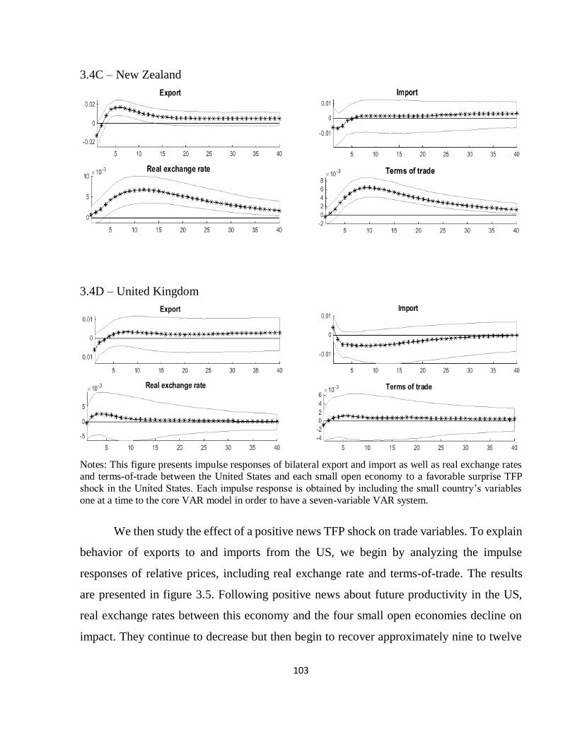
103
3.4C – New Zealand
3.4D – United Kingdom
Notes: This figure presents impulse responses of bilateral export and import as well as real exchange rates and terms-of-trade between the United States and each small open economy to a favorable surprise TFP
shock in the United States. Each impulse response is obtained by including the small country’s variables
one at a time to the core VAR model in order to have a seven-variable VAR system.
We then study the effect of a positive news TFP shock on trade variables. To explain
behavior of exports to and imports from the US, we begin by analyzing the impulse
responses of relative prices, including real exchange rate and terms-of-trade. The results
are presented in figure 3.5. Following positive news about future productivity in the US,
real exchange rates between this economy and the four small open economies decline on
impact. They continue to decrease but then begin to recover approximately nine to twelve

104
quarters after the shock. This fact indicates an appreciation of the US dollar and makes US
goods and services more expensive in the international market. The behavior of the terms-
of-trade is similar to that of the real exchange rates as the terms-of-trade also exhibit J-
shaped impulse responses. These results are also in line with those of Nam and Wang
(2015). In conclusion, the appreciation of the US dollar and the decline of terms-of-trade
make US goods and services less competitive, and therefore favors the export of its trading
partners.
Figure 3.5 Impulse responses of trade and relative price variables in small open economies
to a news TFP shock in the United States
3.5A – Australia
3.5B - Canada

105
3.5C – New Zealand
3.5D – United Kingdom
Notes: This figure presents impulse responses of bilateral export and import as well as real exchange rates
and terms-of-trade between the United States and each small open economy to a favorable news TFP shock
in the United States. Each impulse response is obtained by including the small country’s variables one at a time to the core VAR model in order to have a seven-variable VAR system.
Following a favorable news TFP shock, exports from Canada and the United
Kingdom to the US increase by 4.5% and 4%, respectively, on impact. These effects persist
significantly. However, in the cases of Australia and New Zealand, exports positively
deviate from the trend from the fifth quarter and twelfth quarter, respectively. The
difference between the two groups of countries is explained by the fact that the US is the
first export market of Canada and the United Kingdom (see Table 3.1). Moreover, these
two countries are geographically closer to the US than Australia and New Zealand. Hence,

106
the exports of these two countries to the US react faster and more strongly to macro
fluctuations in the US economy. The increase in exports to the US is explained by the
economic boom generated by the news TFP shock as well as by the fact that goods and
services from these small countries become more competitive due to the effects of the shock
on real exchange rates and terms-of-trade. The responses of imports from the US to these
small open economies are similar to that of exports, except for Australia, wherein the effect
of the shock on the import is not significant until quarter 26. The increase in imports is
explained by the fact that the economic boom in the US is transmitted to these economies
and therefore favors domestic demand. With a significant increase in bilateral trade, the
news TFP shock is transmitted across countries and hence generates business cycle
comovement. In the following section, we investigate the responses of macro aggregate
variables in the small open countries.
3.4.3. Responses of Macro Aggregates of Small Open Countries following
Surprise and News TFP Shocks
Figure 3.6 illustrates the impulse responses of macro-economic variables in four advanced
small open economies following a surprise TFP shock in the US. More specifically, the
GDP of Australia, Canada and New Zealand exhibit a slight decline on impact before
recovering rapidly to the initial levels. The effect of the shock on GDP is not significant in
the case of United Kingdom due to the relative size between the UK and the US in
comparison with other small open economies (See Table 3.3). In general, the surprise TFP
shock generates a small decrease in GDP for four to five periods due to the collapse of
exports from these countries to the US. The impulse responses of consumption in small
economies tell the same story. In the cases of Australia and the United Kingdom,
consumption increases slightly (about 0.2%) on impact. However, this effect dies out
quickly after three to five quarters. In the cases of Canada and New Zealand, we do not find
any significant effect of the shock on consumption. The behavior of employment is similar.

107
It decreases significantly in the case of Canada but is not significant for other small
countries due to the declines in GDP. Investment increases significantly from the ninth
quarter after the shock in the cases of Australia and Canada. In the case of New Zealand,
the effect of the shock on investment is not significant. Investment in the UK declines
significantly until twelfth quarter after the shock.
In sum, a surprise TFP shock in the US generates only small fluctuations in trading
partner economies. Thus, this shock is not a source of the international business cycle
comovement. This result is consistent with findings of Levchenko and Pandalai-Nayar
(2018).

108
Figure 3.6 Impulse responses of trade and relative price variables in small open economies
to a news TFP shock in the United States
3.6A - Australia
3.6B - Canada
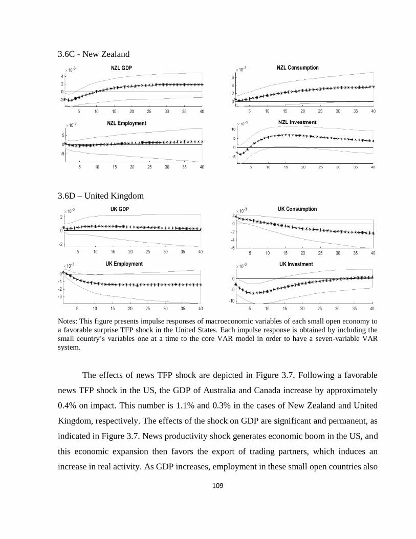
109
3.6C - New Zealand
3.6D – United Kingdom
Notes: This figure presents impulse responses of macroeconomic variables of each small open economy to
a favorable surprise TFP shock in the United States. Each impulse response is obtained by including the
small country’s variables one at a time to the core VAR model in order to have a seven-variable VAR
system.
The effects of news TFP shock are depicted in Figure 3.7. Following a favorable
news TFP shock in the US, the GDP of Australia and Canada increase by approximately
0.4% on impact. This number is 1.1% and 0.3% in the cases of New Zealand and United
Kingdom, respectively. The effects of the shock on GDP are significant and permanent, as
indicated in Figure 3.7. News productivity shock generates economic boom in the US, and
this economic expansion then favors the export of trading partners, which induces an
increase in real activity. As GDP increases, employment in these small open countries also

110
increases, except in the case of New Zealand, where the effect is not significant. The
employment increases by 0.1%, 0.25% and 0.1% in the cases of Australia, Canada and
United Kingdom, respectively. The impact of the news shock on consumption and
investment are similar. These two macro aggregates increase significantly and permanently
after the shock.
To conclude, the effects of news TFP shocks are transmitted across countries by
increasing bilateral trade. In particular, the shock favors the exports from other economies
not only by generating economic booms in the US that increase the demand for foreign
goods but also by making the US goods less competitive in the international market.
Therefore, the economic expansion spills over economies via trade channels. As a result,
news TFP shock is one of important sources of the international business cycle
comovement. These results are summarized in Table 3.2.

111
Figure 3.7 Impulse responses of macro aggregates in small open economies to a news TFP
shock in the United States
3.7A – Australia
3.7B - Canada

112
3.7C - New Zealand
3.7D – United Kingdom
Notes: This figure presents impulses responses of macroeconomic variables of each small open economy to
a favorable news TFP shock in the United States. Each impulse response is obtained by including the small
country’s variables one at a time to the core VAR model in order to have a seven-variable VAR system.

113
Table 3.2 Summary of results
United States Australia Canada New Zealand United Kingdom
Surprise
TFP shock
GDP 0.15% / died out at 9th Q slight decrease slight decrease slight decrease not significant
INV not significant significant from 9th Q significant from 9th Q not significant -0.3% / recovered at
12th Q
CON 0.1% / died out at 3rd Q 0.2% / died out at 5th Q not significant not significant 0.2% / died out at 3rd Q
EMP -0.1% / recovered at 6th Q not significant -0.2% / recovered from
25th Q not significant not significant
SHARE 0.03% / died out at 3rd Q - - - -
EXP - significant from 5th to 27th Q -1% / recovered at 2nd Q significant from 3rd to 12th Q not significant
IMP - significant from 7th Q slightly decrease not significant not significant
RER - hump-shaped hump-shaped hump-shaped hump-shaped
TOT - hump-shaped hump-shaped hump-shaped hump-shaped
News
TFP
shock
GDP 0.3% / died out at 35th Q 0.4% / > 40th Q 0.4% / > 40th Q 1.1% / > 40th Q 0.3% / > 40th Q
INV 1.1% / > 40th Q significant from 5th Q significant from 6th Q 1.5% / > 40th Q 1.5% / > 40th Q
CON 0.2% / died out at 25th Q 1% / > 40th Q 0.25% / > 40th Q 0.3% / > 40th Q 0.3% / > 40th Q
EMP 0.3% / died out at 33rd Q 0.1% / > 40th Q 0.25% / > 40th Q not significant 0.1% / > 40th Q
SHARE -0.15% / > 40th Q - - - -
EXP - significant from 5th Q 4.5% / > 40th Q significant from 12th Q 4% / > 40th Q
IMP - significant from 26th Q 4% / > 40th Q 4% / > 40th Q significant from 1st Q
RER - J-shaped J-shaped J-shaped J-shaped
TOT - J-shaped J-shaped J-shaped J-shaped
Notes: This table presents deviations on impact of variables and numbers of periods that impulse responses are still significant; Q: quarter; > 40 th Q:
still significant after 40th quarter; GDP: Real Gross Domestic Product, INV: Real Investment, CON: Real Consumption, EMP: Employment, SHARE:
Share of expenditure on domestic goods, EXP: Export, IMP: Import, RER: Real Exchange Rate, TOT: terms-of-trade.
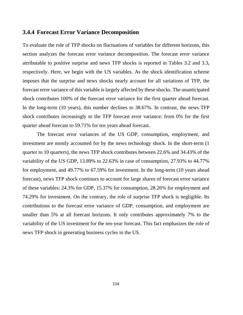
114
3.4.4 Forecast Error Variance Decomposition
To evaluate the role of TFP shocks on fluctuations of variables for different horizons, this
section analyzes the forecast error variance decomposition. The forecast error variance
attributable to positive surprise and news TFP shocks is reported in Tables 3.2 and 3.3,
respectively. Here, we begin with the US variables. As the shock identification scheme
imposes that the surprise and news shocks nearly account for all variations of TFP, the
forecast error variance of this variable is largely affected by these shocks. The unanticipated
shock contributes 100% of the forecast error variance for the first quarter ahead forecast.
In the long-term (10 years), this number declines to 38.67%. In contrast, the news TFP
shock contributes increasingly to the TFP forecast error variance: from 0% for the first
quarter ahead forecast to 59.71% for ten years ahead forecast.
The forecast error variances of the US GDP, consumption, employment, and
investment are mostly accounted for by the news technology shock. In the short-term (1
quarter to 10 quarters), the news TFP shock contributes between 22.6% and 34.43% of the
variability of the US GDP, 13.89% to 22.63% in case of consumption, 27.93% to 44.77%
for employment, and 49.77% to 67.59% for investment. In the long-term (10 years ahead
forecast), news TFP shock continues to account for large shares of forecast error variance
of these variables: 24.3% for GDP, 15.37% for consumption, 28.26% for employment and
74.29% for investment. On the contrary, the role of surprise TFP shock is negligible. Its
contributions to the forecast error variance of GDP, consumption, and employment are
smaller than 5% at all forecast horizons. It only contributes approximately 7% to the
variability of the US investment for the ten-year forecast. This fact emphasizes the role of
news TFP shock in generating business cycles in the US.
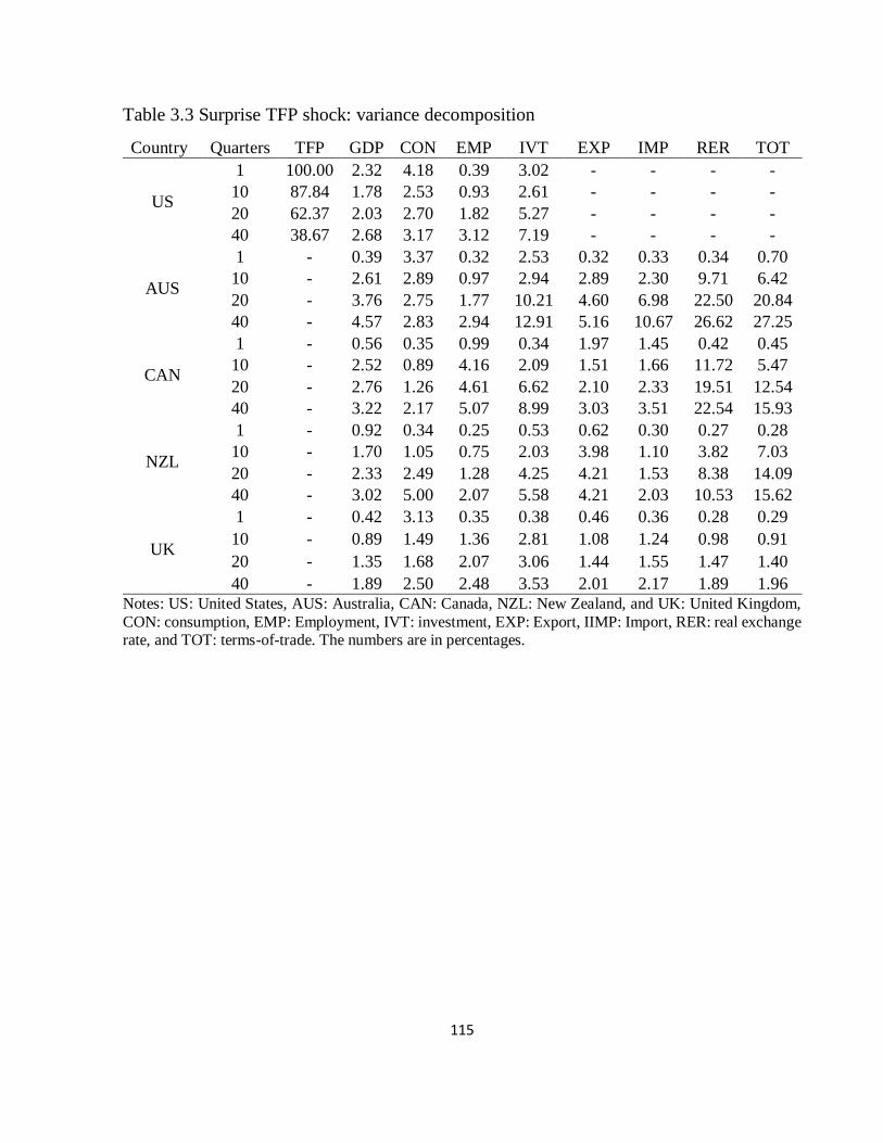
115
Table 3.3 Surprise TFP shock: variance decomposition
Country Quarters TFP GDP CON EMP IVT EXP IMP RER TOT
US
1 100.00 2.32 4.18 0.39 3.02 - - - -
10 87.84 1.78 2.53 0.93 2.61 - - - -
20 62.37 2.03 2.70 1.82 5.27 - - - -
40 38.67 2.68 3.17 3.12 7.19 - - - -
AUS
1 - 0.39 3.37 0.32 2.53 0.32 0.33 0.34 0.70
10 - 2.61 2.89 0.97 2.94 2.89 2.30 9.71 6.42
20 - 3.76 2.75 1.77 10.21 4.60 6.98 22.50 20.84
40 - 4.57 2.83 2.94 12.91 5.16 10.67 26.62 27.25
CAN
1 - 0.56 0.35 0.99 0.34 1.97 1.45 0.42 0.45
10 - 2.52 0.89 4.16 2.09 1.51 1.66 11.72 5.47
20 - 2.76 1.26 4.61 6.62 2.10 2.33 19.51 12.54
40 - 3.22 2.17 5.07 8.99 3.03 3.51 22.54 15.93
NZL
1 - 0.92 0.34 0.25 0.53 0.62 0.30 0.27 0.28
10 - 1.70 1.05 0.75 2.03 3.98 1.10 3.82 7.03
20 - 2.33 2.49 1.28 4.25 4.21 1.53 8.38 14.09
40 - 3.02 5.00 2.07 5.58 4.21 2.03 10.53 15.62
UK
1 - 0.42 3.13 0.35 0.38 0.46 0.36 0.28 0.29
10 - 0.89 1.49 1.36 2.81 1.08 1.24 0.98 0.91
20 - 1.35 1.68 2.07 3.06 1.44 1.55 1.47 1.40
40 - 1.89 2.50 2.48 3.53 2.01 2.17 1.89 1.96 Notes: US: United States, AUS: Australia, CAN: Canada, NZL: New Zealand, and UK: United Kingdom,
CON: consumption, EMP: Employment, IVT: investment, EXP: Export, IIMP: Import, RER: real exchange rate, and TOT: terms-of-trade. The numbers are in percentages.

116
Table 3.4 News TFP shock: variance decomposition
Country Quarters TFP GDP CON EMP IVT EXP IMP RER TOT
US
1 0.00 22.60 13.89 27.93 49.77 - - - -
10 10.74 34.43 22.63 44.77 67.59 - - - -
20 36.64 30.68 20.61 38.99 71.75 - - - -
40 59.71 24.30 15.37 28.26 74.29 - - - -
AUS
1 - 19.89 1.85 1.85 2.80 2.16 6.74 2.38 3.55
10 - 41.28 5.60 15.37 13.74 9.71 12.69 9.98 9.53
20 - 46.79 9.53 17.86 22.74 22.35 13.45 19.22 18.11
40 - 49.54 14.57 21.26 46.43 41.05 21.00 21.12 19.38
CAN
1 - 27.68 13.64 18.29 3.72 38.95 22.58 16.22 15.89
10 - 53.24 30.58 43.11 15.07 51.62 39.71 31.31 19.34
20 - 58.84 40.31 46.10 35.63 52.69 46.68 35.81 19.63
40 - 62.27 51.01 44.50 57.74 55.64 52.89 36.17 22.07
NZL
1 - 38.84 10.54 46.56 20.44 3.74 4.89 4.89 5.43
10 - 55.65 18.15 48.51 36.15 6.21 18.24 9.74 9.33
20 - 68.20 31.90 48.34 47.57 12.99 25.22 12.38 10.48
40 - 77.09 52.13 51.11 59.22 24.86 32.08 13.71 14.06
UK
1 - 13.62 6.67 2.58 10.38 11.92 6.15 11.44 5.89
10 - 23.80 13.63 24.52 34.26 16.94 20.30 14.99 7.03
20 - 25.52 17.09 32.83 44.02 21.33 27.34 16.28 7.84
40 - 28.11 19.53 38.22 50.71 27.92 33.06 17.67 9.74 Notes: US: United States, AUS: Australia, CAN: Canada, NZL: New Zealand, and UK: United Kingdom,
CON: consumption, EMP: Employment, IVT: investment, EXP: Export, IIMP: Import, RER: real exchange rate, and TOT: terms-of-trade. The numbers are in percentages.
The forecast error variance decompositions of small open countries variables
suggests conclusions about the international transmission of shocks. Regarding bilateral
trade and relative price variables, the news TFP shock contributes small shares of variance
at short frequencies, except in the case of Canada. Its contributions to the variance of
exports to the US, imports from the US, real exchange rate and terms-of-trade, on average,
are, respectively, 5.94%, 5.93%, 6.24% and 4.96% for the first quarter forecast. Given the
fact that nearly 70% of Canada’s trade is with the US, the news TFP shock in the US can
substantially explain the forecast variability of the trade and relative price variables of this
economy. At longer frequencies, the role of news TFP shock becomes more important. It
explains 25% to 55% of the forecast error variance of the bilateral export from small open

117
countries to the US, 21% to 53% in the case of the import, 13% to 36% in the case of real
exchange rate, and 10% to 22% in the case of terms-of-trade. Again, the surprise TFP shock
contributes marginally to forecast error variance of the trade variables at all forecast
horizons. Its contributions to bilateral exports and imports are smaller than 5%. However,
the surprise TFP shock accounts for a large share of forecast error variance of the relative
price variables in the long-term, except for United Kingdom, wherein its role is negligible.
The surprise shock is responsible for 26.62% of variance of real exchange rate of Australia
at 10 years. This number is 22.54% and 10.53% in the cases of Canada and New Zealand,
respectively. Surprise shock also explains up to 27.25%, 15.93% and 15.62% of the
variance of the terms-of-trade in the cases of Australia, Canada and New Zealand,
respectively. In sum, while the news TFP shock significantly affects the forecast error
variance of trade and relative price variables, the surprise TFP shock contributes little to
the forecast variability of the former.
Regarding macro aggregates, as reported in Tables 3.2 and 3.3, surprise TFP shock
in the US explains little about the forecast error variance of GDP, employment,
consumption, and investment of the four small open economies. At ten years, it explains
only 4.57%, 3.22%, 3.02% and 1.89% of the GDP forecast variability of Australia, Canada,
New Zealand and United Kingdom, respectively. In contrast, the news TFP shock in the
US accounts for from 14% (Australia consumption) to 77% (New Zealand GDP) of forecast
error variance of the macro aggregates for the ten year forecast. This analysis supports our
findings concerning the importance of news TFP shock in international business cycle
convergence.
3.5. Conclusion
It is important to shed light on how bilateral trade, relative prices (terms-of-trade and real
exchange rate), real activity and other macro aggregates of a small open economy react to
news TFP shocks in its largest trading partner. By using a structural VAR model in which
news TFP shock is identified as in Barsky and Sims (2011), we examine the dynamics of

118
responses of aggregate macroeconomic variables in four advanced small open economies
to anticipated (news) and unanticipated (surprise) TFP shocks in United States. We then
compare the international spillovers of these two shocks. The United States is considered
as the country source that diffuses the shocks because of the relative size of its economy in
comparison with other advanced small open economies as well as its data availability. The
destination countries are four advanced small open economies that trade intensively with
the US: Australia, Canada, New Zealand and United Kingdom.
We provide updated empirical evidence on the responses of the US macro variables
to surprise and news TFP shocks. We indicate that positive news about future productivity
generates economic booms in the US while the surprise productivity shock does not. This
paper reaches two main findings. First, we conclude that the effects of news TFP and
surprise shocks on bilateral trade and relative prices between the US and small open
economies are different. The news shock favors exports to the US not only by generating
economic booms but also by depreciating the US dollar and the terms-of-trade. Second, we
contend that news TFP shocks in the US generate significant macroeconomic fluctuations
and comovement in small trading partners while the surprise TFP shock only causes small
changes. The news TFP shocks are therefore one of the most important sources of the
international business cycle. As a result, countries should focus on bilateral trade with
innovative countries and diffused technology countries in order to benefit from economic
booms generated by the news productivity shock.
Future research may focus on the trade-based news TFP shock transmission between
developed and developing countries. Furthermore, studies could distinguish the responses
in fixed and flexible exchange rate regimes or in countries and regions that sign free trade
agreements. In term of the theoretical side, incorporating news TFP shock may help develop
a new viewpoint regarding the trade-comovement puzzle. That requires further
investigation.
119
References
Barsky, Robert B. and Eric R. Sims. 2011. News shocks and business cycles. Journal of
Monetary Economics 58 (3): 273-289.
Basu, S., Fernald, J.G., Kimball, M.S., 2006, December. Are technology improvements
contractionary? Am. Econ. Rev. 96 (5), 1418–1448.
Beaudry, P., Portier, F., 2004. An Exploration into Pigou’s Theory of Cycles. Journal of
Monetary Economics, 51(6), 1183–1216.
Beaudry, P., Portier, F., 2006, September. Stock prices, news, and economic fluctuations.
Am. Econ. Rev. 96 (4), 1293–1307.
Beaudry, P., Nam, D., Wang, J., 2011, Dec. Do mood swings drive business cycles and is
it rational? NBER Working Papers 17651. National Bureau of Economic Research, Inc.
Beaudry et al., 2013. Comparing Two Methods for the Identification of News Shocks,
Discussion Paper No. 13-110.
Ben Zeev et al. 2017. Emerging economies business cycles: The role of commodity terms-
of-trade news. Journal of International Economics 108 (2017) 368-376.
Fujiwara, I., Hirose, Y., Shintani, M., 2011, 02. Can news be a major source of aggregate
fluctuations? A Bayesian DSGE approach. J. Money, Credit, Bank. 43 (1), 1–29.
Jaimovich, N., Rebelo, S., 2009. Can news about the future drive the business cycle? Am.
Econ. Rev. 99 (4), 1097–1118.
Galí, Jordi. 1999. Technology, Employment, and the Business Cycle: Do Technology
Shocks Explain Aggregate Fluctuations? American Economic Review 89 (1): 249-271.
Kamber G., Theodoridis K. and Thoenissen C., 2017. News-driven business cycles in small
open economies. Journal of International Economics 105 (2017): 77-89.
Juvenal, L., Santos Monteiro, P., 2017. Trade and synchronization in a multi-country
economy. European Economic Review (2017).
Kose, M.A., Yi, K.-M., 2006. Can the standard international business cycle model explain
the relation between trade and comovement? Journal of International Economics. 68,
267– 295.

120
Khan, H., Tsoukalas, J., 2012, December. The quantitative importance of news shocks in
estimated DSGE models. J. Money, Credit, Bank. 44 (8), 1535–1561.
Levchenko and Pandalai-Nayar (forthcoming, Journal of the European Economic
Association). TFP, News, and "Sentiments. The International Transmission of Business
Cycles” (latest version Aug. 2018).
Liao W., and Santacreu A. M., 2015. The trade-comovement puzzle and the margins of
international trade. Journal of International Economics, Volume 96, Issue 2, Pages 266-
288, ISSN 0022-1996.
Nam D. and Wang J. 2015. The Effects of Surprise and Anticipated Technology Changes
on International Relative Prices and Trade. Journal of International Economics 97 (1):
162-177.
Nam, D., Wang, J., 2010. Understanding the effect of productivity changes on international
relative prices: the role of news shocks. Globalization and Monetary Policy Institute
Working Paper No. 61.
Pigou, A., 1927. Industrial Fluctuations. MacMillan, London.
Schmitt-Grohé, S., Uribe, M., 2012. What’s news in business cycles. Econometrica 80 (6),
2733–2764.
Sims E. and Kurmann A. (forthcoming). Revisions in Utilization-Adjusted TFP and Robust
Identification of News Shocks (latest version Nov. 2017).

121
GENERAL CONCLUSION
Business cycle synchronization has been at the center of many debates and has attracted
much attention in contemporary international macroeconomics (Erden and Ozkan, 2014).
Several studies have discussed the existence of a global business cycle and the globalization
and Europeanization of business cycles. Others have examined the transmission of business
cycle through spillover effects. Thus, an important research question asks, what
determinants drive GDP comovement across countries? After the seminal work of Frankel
and Rose (1998), a large body of literature has examined the impacts of trade on
international output correlations. Most studies have confirmed that bilateral trade is one of
the most important determinants of business cycle comovement, among other factors such
as financial integration, industrial specialization, international coordination of monetary
and fiscal policy, foreign direct investment, and firm-level linkages, and exchange rate
regimes. Economies that trade more intensively with each other exhibit a higher output
correlation. As such, this dissertation provides evidence on how and to what extent bilateral
trade influences business cycle comovement. In particular, we add to the existing literature
by developing three empirical essays on the trade-comovement relationship, with specific
focus on the trade spillover effects and macro interdependences in a common currency area,
structure of trade, and the transmission of different types of shock. The three chapters in
this dissertation explore three mechanisms through which trade enhances the output
correlation: demand-supply spillover, technology transmission and terms-of trade effects.
In the first chapter, we investigate the trade spillover effects of the euro area on the
CEECs. By using a near-VAR model that captures direct and indirect effects (through a
third country) of trade over a sample of twelve founding members of the euro area and
seven CEECs from 1996 to 2015, we obtain three notable results. First, three main
economies of the euro area (Germany, France and Italy) have the most important influences
on CEECs though trade channels. Second, trade spillover effects from the euro area to
CEECs are stronger after the European Union enlargement in 2004 (3.3 times larger on
122
average). Finally, and most importantly, the adoption of the euro significantly enhances
responses of CEECs (4.9 for countries that have adopted the euro versus 2.1 for the
countries do not) but does not increase trade intensity (1.07 versus 1.12). The empirical
results also reveal that trade effects on the macro interdependences are positive in the same
currency area but are negative for the CEECs that have not yet adopted the euro. This
chapter focuses on the demand-supply mechanism of trade. Other mechanisms explaining
the positive relation between trade and output correlation include technology transmission
and terms-of-trade effects. Chapter 2 focuses on these two channels to provide further
insight into the trade-comovement puzzle.
According to the trade-comovement puzzle defined in Kose and Yi (2006),
theoretical models fail to fully reproduce the positive impact of trade on business cycle
comovement. The existing literature has suggested that trade at extensive margin transmits
the technology and knowledge embedded in the new products and therefore enhances the
correlation of aggregate productivity between trading partners. A higher correlation of
productivity induces a stronger correlation of output. Juvenal and Santos Monteiro (2017)
have proposed that output correlation may be decomposed into comovement of
productivity, comovement of share of expenditure on domestic goods and comovement of
these two factors. In this chapter, we question whether trade at the extensive margin
generates a pro-cyclical terms-of-trade, thereby increasing the correlation of shares of
expenditure on domestic goods and enhancing business cycle synchronization. By using a
sample of forty countries over the period 1990–2015, we first re-investigate the factor
structure of business cycle comovement proposed by Juvenal and Santos-Monteiros (2017).
Then we test the technology transmission through the extensive margin of trade, as
documented in Liao and Santacreu (2015). Finally, we observe that the extensive margin
of trade is responsible for the comovement of shares of expenditure on domestic goods. Its
effect equals to 0.079 and is significant, at 5%, compared to 0.074 of the effect of overall
trade estimated by Juvenal and Santos Monteiro (2017). The effects of the intensive margin
123
are ambiguous10. That is explained by the fact that when the positive effect of total trade on
shares of expenditure on domestic goods is captured by the extensive margin, the role of
intensive margin is no longer important. In the DSGE model developed by Liao and
Santacreu (2015), the intensive margin generates a counter-cyclical terms-of-trade while
the extensive margin implies a pro-cyclical one. This finding suggests that theoretical
models should integrate the extensive margin of trade in attempt to solve the trade-
comovement puzzle with a technology shock because the extensive margin of trade
generates a pro-cyclical terms-of-trade. Pro-cyclical terms-of-trade is the most important
feature of the model in order to solve the puzzle, as documented in Juvenal and Santos-
Monteiros (2017).
In previous works that have addressed the trade-comovement puzzle, macro
fluctuations are generated from a positive productivity shock. This shock is an
unanticipated, or surprise, shock. However, recent developments in the literature regarding
news (anticipated) shock (Nam and Wang, 2015, Kamber et al., 2017, among others) have
contended that empirical differences exist between the transmissions of news and surprise
productivity shock. Chapter 3 considers the transmission of good news about future
productivity across countries via trade channels. This chapter analyzes trade spillovers of a
news TFP shock in the United States to four advanced small open economies, Australia,
Canada, New Zealand and the United Kingdom. The results obtained from a SVAR model
illustrate that news TFP shocks generate economic booms in the United States (GDP and
Employment increase 0.3% on impact, Investment 1.5% and Consumption 0.2%). This
economic expansion is transmitted to small open countries by increasing their exports to
the United States (export from Canada and United Kingdom to the United States jump up
0.4% and 0.3% on impact, respectively; export from Australia and New Zealand increase
1.5% after 5th quarter and 12th quarter, respectively). Moreover, two reasons explain the
increase in exports of small open economies to the US: demand for final goods in United
States increases following the shock and foreign goods are relatively cheaper due to the
10 These results are robust for some different checks.

124
effects of the shock on real exchange rate and terms-of-trade. In contrast, the effects of
surprise shocks are not significant. Economic booms generated by the surprise shock are
not sufficiently large to be transmitted to trading partners (GDP just increases 0.015% on
impact and dies out at 5th quarter, employment decreases 1% on impact and recovers at the
6th quarter, investment and consumption fluctuations are not significant, and responses of
export from trading partners are not significant or are small). Furthermore, the way surprise
shocks affect the relative price (exchange rate and terms-of-trade) favors US goods. These
results emphasize the role of news TFP shock on international business cycle convergence.
The main contribution of this thesis is to provide more empirical evidence for the
trade-comovement relationship. The three essays help us understand more clearly how
bilateral trade enhances business cycle synchronization in different frameworks and why
theoretical models fail to fully replicate this positive association. This understanding is
important for international policy implications, notably in a common currency area where
trade exchange is highly encouraged, and the high level of business cycle synchronization
assures the efficiency of common economic policies.
125
References
Erden, L., Ozkan, I. 2014. Determinants of international transmission of business cycles
to Turkish economy. Economic Modelling, Volume 36, 2014, Pages 383-390, ISSN
0264-9993.
Frankel, J. A. and Rose, A. K., (1998). The Endogeneity of the Optimum Currency Area
Criteria. Economic Journal, Royal Economic Society, vol. 108(449), pages 1009-25,
July.
Juvenal, L., Santos Monteiro, P., Trade and synchronization in a multi-country economy.
European Economic Review (2017), 97, 385-415.
Kamber, G., Theodoridis, K., and Thoenissen, C., 2017. News-driven business cycles in
small open economies. Journal of International Economics 105 (2017): 77-89.
Kose, M.A., Yi, K.-M., 2006. Can the standard international business cycle model explain
the relation between trade and comovement? Journal of International Economics. 68,
267– 295.
Liao, W., Santacreu, A.M., 2015. The trade-comovement puzzle and the margins of
international trade. Journal of International Economics, Volume 96, Issue 2, July 2015,
Pages 266-288, ISSN 0022-1996.
Nam, D., and Wang, J., 2015. The Effects of Surprise and Anticipated Technology Changes
on International Relative Prices and Trade. Journal of International Economics 97 (1):
162-177.

Titre : Trois essais sur la relation entre le commerce et la synchronisation des cycles économiques
Mots clés : Synchronisation des Cycles Economiques, Transmission des Cycles Economiques, Intégration
Commerciale
Résumé : Ma thèse vise à étudier empiriquement les
effets du commerce sur la synchronisation des cycles économiques. Premièrement, la recherche se concentre sur la relation entre l’intégration commerciale et les interdépendances macroéconomiques au sein de l’Union Européenne. Les résultats obtenus indiquent que l’adhésion à l'Union Européenne et l’adoption de l’euro permettent aux Pays d’Europe Centrale et Orientale d’amplifier les effets du commerce sur l’interdépendance macroéconomique et de s’intégrer plus rapidement à la zone euro. Deuxièmement, la recherche porte sur le puzzle de commerce-synchronisation selon lequel les modèles théoriques sont incapables de reproduire des effets du commerce sur les corrélations du cycle économique aussi forts que ceux estimés par des études empiriques. En décomposant le commerce bilatéral entre la marge intensive et la marge extensive, je trouve que la marge extensive
augmente non seulement la corrélation de la Productivité Global des Facteurs (PGF) entre les partenaires commerciaux mais aussi la corrélation entre les parts de dépenses en biens domestiques. Ce résultat souligne que les nouveaux produits exportés transmettent les chocs de la PGF et ne détériorent pas, voire améliorent, les termes de l'échange. Je suggère donc qu’afin de résoudre le puzzle, il faut que les modèles théoriques intègrent la marge extensive du commerce. Troisièmement, je trouve que les chocs de nouvelle, en combinaison avec le commerce bilatéral, sont une source importante du cycle économique international. Il faut donc que les économies augmentent les échanges avec les pays innovateurs pour profiter les expansions économiques générées par ce type de choc.
Title : Three essays on the relation between trade and business cycle synchronization
Keywords : Business Cycle Synchronization, Business Cycle Transmission, Trade Integration
This dissertation studies the impacts of bilateral trade on business cycle synchronization. First, the chapter 1 examines the relation between trade integration and business cycle interdependences in the European Union. The results obtained indicate that the accession to the European Union and the adoption of the euro enable the Central and Eastern European Countries to amplify the effects of trade on macroeconomic interdependences and to integrate more rapidly into the euro area. Second, the research focuses on the trade-comovement puzzle, according to which theoretical models are unable to replicate trade effects on business cycle correlations as strong as those estimated by empirical studies. By decomposing the bilateral trade into the intensive margin and extensive margin, I find that the
extensive margin of trade not only increases the correlation of Total Factor Productivity (TFP) between trading partners but also increases the correlation between each country's shares of domestic goods. This result emphasizes that new exported products transmit TFP shocks and improve instead of deteriorating the terms-of-trade. Therefore, the extensive margin of trade should be integrated into theoretical models to solve the puzzle. Third, in chapter 3, I find that news TFP shocks, in combination with bilateral trade, are an important source of the international business cycle instead of contemporaneous TFP shocks. As a result, countries should focus on bilateral trade with innovative and technology-diffusing countries in order to benefit from economic booms generated by the news productivity shock.