three essays on syndicated loan partnerships
TRANSCRIPT

Texas A&M International University Texas A&M International University
Research Information Online Research Information Online
Theses and Dissertations
4-29-2020
Three Essays on Syndicated Loan Partnerships Three Essays on Syndicated Loan Partnerships
Bolortuya Enkhtaivan
Follow this and additional works at: https://rio.tamiu.edu/etds
Recommended Citation Recommended Citation Enkhtaivan, Bolortuya, "Three Essays on Syndicated Loan Partnerships" (2020). Theses and Dissertations. 83. https://rio.tamiu.edu/etds/83
This Dissertation is brought to you for free and open access by Research Information Online. It has been accepted for inclusion in Theses and Dissertations by an authorized administrator of Research Information Online. For more information, please contact [email protected], [email protected], [email protected], [email protected].

THREE ESSAYS ON SYNDICATED LOAN PARTNERSHIPS
A Dissertation
by
BOLORTUYA ENKHTAIVAN
Submitted to Texas A&M International University
in partial fulfillment of the requirements
for the degree of
DOCTOR OF PHILOSOPHY
May 2016
Major Subject: International Business Administration

THREE ESSAYS ON SYNDICATED LOAN PARTNERSHIPS
A Dissertation
by
BOLORTUYA ENKHTAIVAN
Submitted to Texas A&M International University
in partial fulfillment of the requirements
for the degree of
DOCTOR OF PHILOSOPHY
Approved as to style and content by:
Chair of Committee, Siddharth Shankar
Committee Members, R Stephen Sears
Anand Jha
George R.G. Clarke
Head of Department, Antonio J. Rodriguez
May 2016
Major Subject: International Business Administration

iii
ABSTRACT
Three Essays on Syndicated Loan Partnerships (May 2016)
Bolortuya Enkhtaivan, M. A., University of Virginia;
Chair of Committee: Dr. Siddharth Shankar
The purpose of this dissertation is to contribute to the syndicated loan literature. More
specifically, this dissertation is composed of three chapters and each chapter explores different
aspects. First, we examine syndicated loan’s structure in the presence of regulatory bail-outs. The
Troubled Asset Relief Program (TARP) was implemented during the 2009 economic downturn
to stimulate the credit flow. However, the low cost of capital could have imprudently increased
lenders’ credit risk-appetite. In three different measures, we find that TARP effectively
prevented moral hazard by its participants as evidenced by the syndicated loans’ more diversified
structures. Further study at lender level suggests that TARP’s impact was heterogeneous. In the
case of TARP participants that are lead arrangers in the syndicate, average bank share has
increased. This result is robust to propensity score matching and instrument variable approaches.
Next, we explore syndicated loan’s terms. We look at how the reputation of lead
arrangers or the auditors might signal the borrower’s credit quality, thus determine loan terms.
We find that when the borrower has either reputable lead arrangers or Big 4 auditors, it benefits
by receiving more favorable terms. Loan amount increases, maturity extends while interest
spread narrows and the number of financial covenants decreases. If the borrower has both, it is
even better. An average borrower who has a Top 10 lead arranger and a Big 4 auditor at the same

iv
time could reduce its loan price by about 37bps, the number of financial covenants by about 0.2
units and increase loan amount and maturity materially by about 121.3 million USD and a year
respectively.
Finally, we focus on lender’s role in the syndicate. The research question here is which
banks have a higher chance of receiving lead mandates? The results based on logistic regression
show that the past relationship with the borrower increases that bank's odds of winning the lead
mandate by 34%. Moreover, while being a top 10 lender increases the odds of winning the lead
mandate by 21%, specialization in the borrower’s industry increases it by even more, at 47%.
When we handle the identification problem, results improved significantly.

v
ACKNOWLEDGEMENTS
I owe my gratitude to all those people who have made this dissertation possible and
supported me throughout the pursuit of my doctoral degree. My deepest gratitude goes to my
advisor, Dr. Siddharth Shankar, who has guided me in my research, dedicated his valuable time
for me and has been there for me willing to listen and support my every endeavor.
I sincerely thank Dr. Stephen R. Sears who is very supportive of high-quality academic
researches and encourage doctoral students by all means. His financial support for the Dealscan
data made this dissertation possible. Also, the recognitions of doctoral student best papers at
Western Hemispheric Trade Conferences (WHTCs) promote scholarly works and provide
opportunities to improve.
I am indebted to my other committee members Dr. Anand Jha and Dr. George Clarke for
their insights, constructive criticisms, and suggestions to improve the methodologies. I greatly
enjoyed open discussions with Dr. Jha exploring research ideas and developed new research
skills and programming while working as his research assistant. I am grateful to Dr. Clarke in
organizing WHTCs effectively that facilitated to network, learn and grow professionally.
Very special thanks go to my husband, Zagdbazar Davaadorj, who has been always there
to help. From developing the research ideas to hand matching the data, running the analyses,
writing, discussing, presenting and editing he was the ear to listen, the eye to see, the arm to
assist and the inspiration to move on.
Finally, I have benefited greatly from the feedbacks of conference participants in
Midwest Finance Association 2015, Eastern Finance Association 2015 & 2016, Southwestern

vi
Finance Association 2015 & 2016, Western Hemispheric Trade Conference 2015 & 2016 and the
participants at the research seminar series at Texas A&M International University.
vii
TABLE OF CONTENTS
Page
ABSTRACT ................................................................................................................................... iii ACKNOWLEDGEMENTS .............................................................................................................v
TABLE OF CONTENTS .............................................................................................................. vii LIST OF TABLES ......................................................................................................................... ix INTRODUCTION ...........................................................................................................................1 CHAPTER
I INTERVENTION OF REGULATORY BAILOUTS IN LOAN PARTNERSHIPS:
EVIDENCE OF TARP'S EFFECT ON SYNDICATED LOAN STRUCTURE ................8 Introduction ............................................................................................................... 8
Literature review and hypotheses development ...................................................... 13
Measurement of variables and construction of the empirical model ...................... 17 Measuring syndicated loan’s structure ........................................................... 17 Measuring TARP variable .............................................................................. 17 Measuring control variables ........................................................................... 18
Empirical model development ........................................................................ 24 Data ......................................................................................................................... 25
Results ..................................................................................................................... 29 Summary statistics .......................................................................................... 29 Diagnostic tests ............................................................................................... 30
Multivariate regression results ........................................................................ 33 Additional analysis and robustness check ............................................................... 39
Instrumental variable analysis ........................................................................ 39 Propensity score matching .............................................................................. 41
Subsample analysis ......................................................................................... 43 Conclusion .............................................................................................................. 44
II THE CERTIFICATION EFFECT ON LOAN TERMS ....................................................46 Introduction ............................................................................................................ 46 Literature and hypotheses development................................................................. 50
Top lead arranger and loan terms .................................................................. 50 Big 4 auditor and loan terms.......................................................................... 51 Contribution to the literature ......................................................................... 52
Hypotheses development ............................................................................... 53 Model development and data ................................................................................. 54
Empirical model ............................................................................................ 54 Measuring key variables ................................................................................ 55
Main results ............................................................................................................ 62 Certification effect decreases loan spreads .................................................... 62
Certification effect increases loan amounts ................................................... 65
Certification effect increases loan maturity ................................................... 66 Certification effect decreases loan financial covenants ................................. 66
Robustness tests ..................................................................................................... 67 Alternative estimation method ...................................................................... 67 Alternative measures for certification .......................................................... 68

viii
Page
i
Conclusion ............................................................................................................ 68 III DO PAST RELATIONSHIP AND EXPERIENCE HELP A BANK IN WINNING A
LEAD MANDATE IN THE SYNDICATED LOAN BID?..............................................70 Introduction ........................................................................................................... 70 Literature and hypotheses development................................................................ 74
Financial strength hypothesis ...................................................................... 74 Hypotheses on past behaviors ...................................................................... 75
Data and variables ................................................................................................. 76 Sample construction .................................................................................... 76 Dependent variable ...................................................................................... 77
Bank behavioral variables ........................................................................... 77 Bank financial variables .............................................................................. 78 Loan variables .............................................................................................. 79
Methodology ......................................................................................................... 80 Results and discussions ......................................................................................... 82
Robustness tests .................................................................................................... 89 Dealing with selection bias .......................................................................... 89 Alternative measures for behavioral variables ............................................ 91
Conclusion ............................................................................................................ 93 REFERENCES ..............................................................................................................................95
APPENDIX
VARIABLE DEFINITION .............................................................................................101
VITA ..........................................................................................................................................105

ix
LIST OF TABLES
Page
Table 1.1 Summary statistics ........................................................................................................ 28
Table 1.2 Pearson's correlations .................................................................................................... 31
Table 1.3 T-test results .................................................................................................................. 32
Table 1.4 Results from loan level analysis ................................................................................... 34
Table 1.5 Lender level regression analysis ................................................................................... 38
Table 1.6 Instrumental variable analysis for endogenous TARP variable .................................... 40
Table 1.7 Results for propensity matched samples ....................................................................... 42
Table 1.8 Results for restricted sample with at least one lead bank ............................................. 45
Table 2.1 Top 10 lead arrangers ................................................................................................... 57
Table 2.2 Summary statistics and Pearson's correlations.............................................................. 60
Table 2.3 Main regression results ................................................................................................. 63
Table 2.4 Summary of main results .............................................................................................. 65
Table 2.5 Robustness test: comparison with SUR estimation method ......................................... 68
Table 3.1 Descriptive statistics and Pearson’s correlations .......................................................... 83
Table 3.2 Main results................................................................................................................... 86
Table 3.3 Pre and post crisis periods ............................................................................................ 89
Table 3.4 Subsample analyses ...................................................................................................... 92
Table 3.5 Behavioral variables as measured by the number of deals ........................................... 94

1
INTRODUCTION
A syndicated loan is a type of loan in which several lenders come together with a purpose
of issuing a loan to a single borrower under the same contract. Syndicated loan process starts
with a borrower’s loan request from its preferred bank which often becomes a lead bank of the
syndicate. The lead bank conducts due diligence, evaluates borrower’s risks and arranges
additional funds required by inviting other participants. Shared National Credit Program under
Federal Reserve System defines loans shared by more than three supervised institutions
amounting over $20 million as large syndicated loans and requires periodic review by the
Reserve Banks.
Syndicated loan market has grown both in size and importance over the years. The U.S.
market alone has grown multifold in recent years due to expanding corporate activities and better
access to global funding market. As of 2014 syndicated loan outstanding balance stands at $1.57
trillion (46.3 percent of the total commitment of $3.39 trillion) which is 6.4 times larger (and 4.9
times larger in total commitments) than that of in 1989 (Board of Governors of the Federal
Reserve System (2014)). Moreover, due to complexities and various incentives involved in
syndicated loan process different types of institutions actively participate in U.S. syndicated loan
market. Out of total syndicated loan commitments, U.S. banks constitute 44.4%, foreign banks
constitute 35.8%, and non-banks constitute 19.7% respectively as of 2013, and the statistics
remain stable in 2014 (Board of Governors of the Federal Reserve System (2014)). Non-bank
institutions include institutional investors such as securitization pools, hedge funds, and
insurance funds.
This dissertation follows the style of the Journal of Finance.

2
Lenders form syndication for different reasons and incentives. As compared to a sole-
lender loan, a syndicated loan limits credit risk exposures for an individual lender by spreading
out the credit risk among several participants. In addition to limited credit risk exposure,
syndication also provides an opportunity for new business development, extra profits from non-
traditional fees and efficient asset allocation (Campbell and Weaver (2013)). Consequently, a
decision whom to partner with highly depends on lenders’ motives as well as potential partners’
strengths and weaknesses. Furthermore, from the borrower’s perspective, obtaining syndicated
loan not only has an advantage of diversifying lenders’ commitment risks (Campbell and Weaver
(2013)), but also builds relationships with other lenders. Therefore, behaviors of the parties in the
syndicated loan offer a promising area for research.
Agency theory explains cooperative behaviors of syndicate parties. While the borrower
knows its credit quality lenders may not have the same information raising an issue of
information asymmetry. Due to nature of multiple lenders participating in the syndicate, the
degree of information asymmetry is not uniformly distributed. Lead arrangers either through
their past relationships or syndication responsibilities that require more frequent engagements
with the borrower have access to borrower’s private information. Possession of private
information makes lead banks susceptible to adverse selection and moral hazard problems
(François and Missonier-Piera (2007)).
Adverse selection problem arises due to the possibility that lead arrangers issue loans to
low-quality borrowers. Furthermore after issuing the loan, lead arrangers may not put the
adequate effort in monitoring activities which may create moral hazard problem. Therefore,
agency theory suggests retaining of larger shares of the syndicate by lead arrangers could
mitigate the agency problem. Furthermore, when lead lenders retain larger shares, it alleviates

3
free-riding incentives of other participants on lead lenders’ costly monitoring. Sufi (2007)
supported the agency theory hypotheses and according to his findings geographic proximity and
past relationships with the borrower reduce information asymmetry, thus agency problems.
Growing number of studies in the area of loan syndication have focussed in explaining
different features of the loan syndication, determinants of the syndicate structure, lender-
borrower relationships as well as lenders’ partnering behaviors. Champagne and Kryzanowski
(2007) find that past cooperation is a significant determinant of future cooperation in the
syndicate and the relationship last longer if the roles in the syndicate remain the same. Their
findings are consistent with specialization theory (François and Missonier-Piera (2007)).
Moreover, the reputation of lead arrangers plays a significant role in signaling screening and
monitoring capacity, so it reduces information asymmetry. Ross (2010) finds favorable market
reactions to the announcement of dominant bank involvement in the syndicated loan and market
reaction strengthens when the borrower has fewer disclosure requirements.
Furthermore, Gopalan, Nanda and Yerramilli (2011) study partnering behaviors of
lenders in case of borrower bankruptcies. Their findings suggest that although borrower
bankruptcies result in hardships for lead arrangers to attract partners in the future, for dominant
players, impacts are not significant. Besides supply factors, overall economic condition
determines the syndicated loan’s structure. Anil and Wei-Ling (2011) study syndicated loan’s
structures in different business cycles. They find evidence of increased risk appetite and weaker
monitoring of borrowers during the growth period. Moreover, consistent with Sufi (2007) they
find more relaxed monitoring from lead arrangers when the loan is more diversified with a larger
number of participants. Moreover, Mariassunta and Luc (2012) look at the participation of

4
foreign lenders in the syndicate in different business cycles. They observe shifts of foreign
partners to their home countries withdrawing from loans in bad times.
Despite a large number of studies in the syndicated loan market, complex nature of
behaviors involving significant parties grants a lot of room for further studies. The purpose of
this dissertation is to contribute and expand the syndicated loan literature in multiple directions.
More specifically, the dissertation is composed of three chapters, and each chapter explores
different attributes of the syndicated loan. In chapter 1, we examine syndicated loan’s structure,
in chapter 2 we explore syndicated loan’s terms and finally in chapter 3 we look at the lender’s
roles in the syndicate respectively.
Syndicated loan’s structure is defined as the composition of lenders in the syndicate and
highly depends on the lenders’ incentives to share risks. Common measures for the syndicated
loan structure include the number of lenders syndicate, the number of lead arrangers, average
bank share and Herfindahl-Hirschman Index. Lenders’ risk-sharing incentives, so does the
syndicated loan’s structure can be explained by the borrower’s transparency (Sufi (2007)),
corporate ownerships (Lin, Ma, Malatesta and Xuan (2012)) and financial well-being (Gopalan,
Udell and Yerramilli (2011)). Moreover, several other studies (Cai (2009), Champagne and
Kryzanowski (2007)) document that past loan alliances among lenders significantly impact
future loan alliances. Beyond borrower and lender factors overall economic conditions impact
the syndicated loan’s structure as evidenced in Anil and Wei-Ling (2011) and Mariassunta and
Luc (2012).
In chapter 1, we examine syndicated loan’s structure in the presence of regulatory bail-
outs under the Troubled Asset Relief Program (TARP). While the purpose of TARP was to
stimulate the flow of credit during the economic downturn, the low cost of capital could have

5
functioned as a double-edged sword by imprudently increasing lenders’ credit risk-appetite. The
analyses reveal two important findings: first, we find that while TARP provided low-cost
funding during the crisis, it effectively prevented moral hazard by its participants as evidenced
by the syndicated loans’ more diversified structures. This result is evident in three different
measures of syndicated loan’s structure.
Furthermore, the lender-loan level analyzes suggest that TARP’s impact varied across
lender groups. Although we find that TARP diversified syndicated loans’ structure in general, it
increased loan concentration among lead arrangers. We argue that in recessionary periods the
necessity of credit monitoring reaches its peak. Therefore, the agents responsible for such
strengthened credit monitoring would require greater rewards. Thus, in the case of syndicated
loans lead arrangers who conduct the credit monitoring would retain larger shares from the loan
in lieu of compensations. The result is robust to propensity score matching, instrument variable
analysis, alternate variable measures, and subsample analysis.
In chapter 2, we explore various loan terms in the syndicated loans—the yield spread,
loan maturity, loan size and loan covenants. We examine the role of lead arranger’s reputation in
negotiating these loan terms. We argue that an involvement of reputable lead arranger conveys
valuable information to the information disadvantaged syndicate participants about the true
quality of the borrower. So-called certification effects of reputable lead arrangers have been
evidenced in the syndicated loan literature and benefited borrowers in reducing their credit costs.
However, little has been explored about certification effect beyond loan price terms. An equally
interesting question for borrower would be benefits of having reputable lead arrangers in
negotiating other non-price loan terms.

6
Our results support the certification effect by finding more favorable loan terms for the
borrower in the presence of Top 10 lead arrangers. While loan spread tightens and the number of
financial covenants reduces loan maturity and amounts increase. Extending the added value of
certification effect with the presence of borrower’s reputable (Big 4) external auditors, results
become even stronger. An average borrower who has a Top 10 lead arranger and a Big 4 auditor
at the same time could reduce its loan price by about 37bps, number of financial covenants by
about 0.2 units and increase loan amount and maturity materially by about 121.3 million USD
and a year longer respectively. The results are robust to SUR estimation method after we allow
correlations among dependent variables and use different measures for certification. Overall,
results suggest that even for top tier lenders who possess higher monitoring capacity, an
independent third party certification could add informational value.
Finally in Chapter 3, we explore lender’s role in the syndicated loan. Little is known
about how borrowers select lead arrangers in a syndicated loan. The purpose of this chapter is to
examine the significance of the private-linkages and the bank experience in granting a lead
mandate. The results based on logistic regression show that the past relationship with the
borrower increases that bank's likelihood of winning the lead mandate by 34%. Moreover, while
being a top 10 lender increases the probability of winning the lead mandate by 21%,
specialization in the borrower’s industry increases it by even more, at 47%.
Furthermore, the sub-sample analysis demonstrates that results are mainly driven by the
pre-crisis period, implying that borrowers prefer single bidders rather than bidding groups when
funding is abundant. Analyses focusing on above median Tier 1 capital and above median total
assets further validate these results with the effect being even stronger as these groups represent

7
reasonable candidates for bidding invitations. Finally, alternative measures for behavioral
variables indicate that borrowers emphasize lenders’ quality over quantity.
8
CHAPTER I
INTERVENTION OF REGULATORY BAILOUTS IN LOAN PARTNERSHIPS:
EVIDENCE OF TARP’S EFFECT ON SYNDICATED LOAN STRUCTURE
1.1 Introduction
When several lenders partner with each other to issue a loan to a single borrower under
the same contract, they form a loan syndicate. A syndicated loan has become common practice
around the world and is frequently used for various corporate purposes. The US market alone has
grown significantly in recent years due to expanding corporate activities and better access to the
global funding market. As of 2014, the total outstanding balance of syndicated loans stood at
$1.57 trillion (46.3% of the total commitment of $3.39 trillion), which is 6.4 times larger (and
4.9 times larger in total commitments) than that of 1989 (Board of Governors of the Federal
Reserve System (2014)).
The syndication starts when a borrower requests a loan from its preferred bank, which
often plays the lead arranger role in the syndicate. The lead arranger conducts due diligence,
evaluates the borrower’s risks, supplies additional funding by inviting other participants,
mediates loan agreements, channels loan repayments, monitors borrowers, and solves any
disputes throughout the loan’s life. Because of these multiple functions and depending on the
scope of the borrower’s business and its geographical location, several lenders might share the
lead arranger’s responsibilities or offer other parties to be in charge of functional duties. As a
result syndicated loan’s structure may be either concentrated or diversified in terms of a number
of lenders, the number of lead arrangers, average bank’s share in the syndicate or the Herfindahl-
Hirschman Index of loan concentration.

9
Both the lenders and the borrower follow their incentives and agree on structuring a
syndicated loan due to several advantages it offers. The main advantage is the large size of a
loan. Thus, as compared to a sole-lender loan, a syndicate has the advantage of limiting the
exposure to credit risks for an individual lender by sharing responsibility with other participants.
Also, Campbell and Weaver (2013) list profits from nontraditional fees, new business
development opportunities, and efficient asset sources as other attractions to syndications.
Consequently, a decision on who to partner with depends highly on the lender’s motives as well
as its potential partners’ strengths and weaknesses. Furthermore, from the borrower’s
perspective, obtaining a syndicated loan not only has the advantage of diversifying the lenders’
commitment risks (Campbell, and Weaver (2013)) but also of building relationships with other
lenders while meeting its large scale funding needs. Therefore, the behaviors of the agents in a
syndicated loan offer a promising case study for research.
The agency theory explains the cooperative behaviors of syndicate parties. While the
borrower knows its credit quality, the lenders might not have the same information. Thus,
information asymmetry becomes an issue. Due to the nature of the syndicate’s multiple lenders,
the degree of information asymmetry among them is not uniformly distributed. The lead
arrangers, either through their past relationships or the syndicate’s responsibilities that require
more frequent engagements with the borrower, have access to more of the borrower’s private
information. The possession of private information makes the lead arrangers susceptible to
adverse selection and moral hazard (François and Missonier-Piera (2007)). Adverse selection
arises from the possibility that the lead arrangers will issue loans to low-quality borrowers.
Moreover, after the loan’s issuance, the lead arrangers might not put adequate effort into
monitoring, thus creating a moral hazard problem. Therefore, the agency theory suggests that the

10
lead arrangers with larger shares of the syndicate could align their incentives with the other
lenders to avoid these problems. Furthermore, when lead arrangers obtain larger shares, these
shares alleviate the incentives of other participants to free-ride on the lead arrangers’ costly
monitoring. Sufi (2007) supports the agency theory and finds that the geographic proximity and a
past relationship with the borrower reduce the information asymmetry, and thus agency
problems.
A growing number of studies are dedicated to explaining the different features of loan
syndicates, determinants of their structure, lender-borrower relationships, as well as lenders’
partnering behaviors. For example, Champagne and Kryzanowski (2007) highlight importance of
past cooperation among lending partners in determining a future syndicate cooperation. Their
evidence suggests longer lasting relationship when the roles of partners remain the same in the
future syndicate consistent with the specialization theory (François and Missonier-Piera (2007)).
Moreover, the reputation of the lead arrangers plays a significant role in signaling the screening
and monitoring capacity of the leads, which reduces information asymmetry. Ross (2010) finds
favorable market reactions to the announcement of a dominant bank’s involvement in the
syndicated loan, and the impact is strengthened when the borrower has fewer disclosure
requirements. Similarly, Gopalan, Nanda and Yerramilli (2011) study the behaviors of lending
partners in the case of borrowers’ bankruptcies. Their findings suggest that although the
borrowers’ bankruptcies make it harder for the lead arrangers to attract partners in the future, for
dominant players, the impact is not significant.
Besides aforementioned lender and borrower-related factors, the overall economic
condition determines the syndicated loan’s structure. Anil and Wei-Ling (2011) study syndicated
loan structures in different business cycles. They find evidence of increased risk appetite and

11
weaker monitoring for borrowers during growth periods. Moreover, consistent with Sufi (2007)
they find more relaxed monitoring from lead arrangers when the loan is more diversified with a
larger number of participants. Moreover, Mariassunta and Luc (2012) look at the participation of
foreign lenders in the syndicate in different business cycles. They observe that foreign partners
shift to loans in their home countries during bad times. Defined as the flight-home effect such
resource shift significantly reduces the capital supply, increases liquidity needs and borrowing
costs exacerbating the domestic market’s condition.
However, a regulatory intervention such as the recent Troubled Asset Relief Program
(TARP) implemented by the U.S. government during the 2008 subprime mortgage crisis may
change the story completely as it provided a massive bailout of $475 billion. The purpose of
TARP and its five different programs was to stimulate lending and restore credit flow in the
economy. Among these programs, the Capital Purchase Program (CPP) intended to rescue banks
by injecting the necessary capital during the crisis. The CPP spent $204.9 billion of TARP’s
funding for the capital injections. The Treasury reports that TARP was successful in terms of
repayment because it received $221 billion in total in the form of equity buyback, dividend,
interest, and other income from its 707 participants. Several studies explore the impact and
efficiency of TARP empirically, and their findings show mixed results. Some argue that TARP
played a significant role in stabilizing the economy by restoring the investors’ confidence (Gaby
and Walker (2011), Huerta, Perez-Liston, and Jackson (2011), Yildirim and Pai (2012)),
improving the stock markets’ performance (Hollowell (2011)), increasing credit supply (Li
(2013)) and strengthening bank’s competitiveness (Berger and Roman (2013)). However, others
emphasize the possibility that TARP stimulated the opportunistic behavior of banks by offering
the option of less costly funding (Cornett, Li and Tehranian (2013)). These studies find some

12
evidence of deteriorated operating efficiencies in TARP participants (Harris, Huerta and Ngo
(2013)).
Although many studies explore the impact of TARP at different levels, to best of our
knowledge none has investigated its effect at loan level yet. The purpose of this paper is to fill
this gap by empirically examining the syndicated loan structure that was formed during the
financial crisis period with TARP support. Depending on the bailout conditions and regulatory
monitoring’s stringency, the banks chose optimal risk levels. Low cost of bail-out resource could
have functioned as a double-edged sword by imprudently increasing lenders’ credit risk-appetite
under the name of a credit supply improvement. If TARP was efficient in creating flows of
funds while preventing moral hazard in its recipient banks during the financial crisis, then the
TARP loans should be more diversified.
If efficiency were the case, we argue that with funding from TARP, the Federal Reserve
banks must have closely monitored the recipients, and the recipients maintained less
concentrated risk exposures. Therefore, the syndicate’s structure was formed with a larger
number of total banks and a larger number of total lead arrangers in which the lead banks have
smaller mean shares and a lower overall Herfindahl-Hirschman Index (HHI) of concentration as
compared to non-TARP loans. The study contributes to the literature in two ways. First, it
explains partnering behaviors in loan syndicates when there is a regulatory shock. Second it
evaluates the effectiveness of TARP in terms of promoting cooperative lending and risk-sharing
while providing funding flows.
Indeed, our results support that TARP promoted more diversified syndicated loan
structure for three different measures of the syndicate structure. We find a positive and

13
significant effect of the TARP loan dummy on the number of banks that indicates that if there is
a TARP recipient in the syndicate, then its structure becomes more diversified. Moreover, we
find a negative association between TARP loan dummy and average bank share in the syndicate
and the HHI of the loan syndicate further validating the diversified syndicated loan structure.
The results hold for an alternative measure of average TARP infusion rate for the loan and
consistent in various subsample tests.
Furthermore, when we segregate TARP’s impact by the lender group based on their roles,
we find an interesting result. While TARP diversified syndicated loan structure in general, it
increased the concentration among lead arrangers. The results remain robust to several additional
tests including instrumental variable approach and propensity score matching. Our paper is
organized as follows: Section 1.2 discusses the literature and develops the hypotheses; Section
1.3 describes the measurement of variables and construction of the empirical model; Section 1.4
describes the data; Section 1.5 provides results; Section 1.6 checks the validity of the main
results and reports additional robustness test results, and Section 1.7 concludes.
1.2 Literature review and hypotheses development
The theories on bank regulation build on the financial market’s imperfection and the
essentials of intervention to minimize negative externalities. Systemic crisis prevention is the
major argument to support bank regulation. Banks are exposed to liquidity risk because of the
mismatch between liquid assets and demand deposits. Diamond and Dybvig (1983), Gorton
(1985), and Chari and Jagannathan (1988) were the first to model pure panic runs where
depositors withdrew simultaneously. In the absence of proper policies, the market fails to meet
rapid liquidity needs, and smooth transaction flows become distorted. Consequently, this severe
condition initiates further domino effects that cause a systemic crisis (Allen and Gale (2000),

14
Kodres and Pritsker (2002)). Therefore, regulatory intervention becomes one of the solutions to
avoid social distress.
Furthermore, recent theory (Santos (2001)) suggests that the banks’ monitoring role is a
rationale for regulation. The individual depositors’ small share makes it costly for them to
monitor banks and promotes free-riding. When deposit insurance exists, depositors are no longer
concerned about controlling the banks’ risk-taking (Diamond and Dybvig (1983), Diamond and
Dybvig (1986)). Moreover, the deposit insurance might raise potential moral hazard in the banks
in terms of an excessive risk appetite if they pay flat premiums. The situation worsens in the case
of management that is separate from its owners, initiating corporate government problems.
Therefore, independent monitoring from a regulatory authority fulfills the need to support
stability. Common bank regulation practices include regulatory capital requirements along with
other prudential constraints and periodic disclosure mandates.
Therefore, besides the periodic monitoring of banks, regulators intervene in the market as
needed for the purpose of promoting the stability of the banking sector and preventing any
potential contagion. During the economic downturn in 2008, the US Congress enacted the
Emergency Economic Stabilization Act to supply $700 billion through the Troubled Asset Relief
Program (TARP). The initial commitment amount was reduced to approximately $475 billion,
and $205 billion was authorized to CPP. As of March 2013, the initial injection had been fully
recovered with a $3.3 billion loss. The active outstanding amount is only $6.8 billion (Treasury
(2013)). A total of 707 financial institutions participated in the program while the number of
applications to the TARP program overall was well above that. Some evidence suggests that
banks considered TARP as an option for less costly funding (Cornett, Li and Tehranian (2013)).

15
One of the reasons behind the recent crisis was the excessive risk-taking of banks and
institutional investors. TARP attempted to limit risk exposure and restrict executive
compensation for banks that sought TARP money. Consequently, a research stream emerged to
study the TARP restrictions on executive compensation. For example, Bayazitova and
Shivdasani (2012) and Cadman, Carter and Lynch (2012) argue why restrictions on the executive
compensation would discourage firms from participating in the CPP. Further, Black and
Hazelwood (2012) examine the impact of TARP’s conditions on executive compensation to
restrict risk-taking behaviors. They find that risk-taking behavior is highly related to the bank’s
size. While larger banks increase their risk-taking commensurately with the credit stimulation,
smaller banks reduce their risk-taking as a result of the restrictions on executive compensation.
Similarly, Kim and Stock (2012) find that TARP affects executive compensation, firms’
performances, the capital structure of banking firms at the micro-level; and the stock market’s
stability and the financial system at the macro-level.
Another research stream on TARP explores its impact and efficiency. Harris, Huerta and
Ngo (2013) find evidence of moral hazard of TARP participants. Their non-parametric analysis
results demonstrate deteriorated operating efficiency for TARP banks as compared to non-TARP
banks. In contrast to that Gaby and Walker (2011) conclude overall TARP has been effective in
restoring confidence in the U.S. financial system. Further, the long-term stock performance of
TARP recipients outperformed their non-TARP counterparts (Hollowell (2011)). With the same
token, Huerta et al. (2011) and Yildirim and Pai (2012) argue that TARP bailouts regained
investor confidence in the market and as a result the stock market volatility and investors’ fear
decreased. Similarly, according to Li's (2013) estimation capital inadequate banks were able to
increase their annualized loan supply with TARP funding by 6.36 percent which directly

16
translates into $404 billion at the macro level. Further evidence suggests that TARP was
effective at individual bank level as well by strengthening market power measured by Lerner’s
index (Berger and Roman (2013)) and increasing loan issuance while meeting regulatory capital
requirement (Taliaferro (2009)).
In line with TARP supporters, we hypothesize that TARP was effective in promoting risk
diversification at loan level. More specifically, we propose:
H1.1: TARP effectively promoted credit flow while at the same time limited credit risks, so at the
syndicated loan level the funds resulted in a more diversified syndicate structure.
Lead arrangers in the syndicated loan play crucial roles. They are the ones that originate,
arrange, price, underwrite and structure the deal based on the borrower-specific needs. As
explained in Campbell and Weaver (2013) in detail lead arranger candidates propose their
underwriting methods in the lead mandate bids. They specify whether the deal will be wholly or
partially underwritten or best effort deal. When the deal is wholly underwritten, the lead arranger
grants the complete deal amount regardless of how much funding was raised in the market it will
be in charge of the remaining amount. If instead, the deal is partially underwritten, it will be in
charge of the portion specified in the agreement. Finally, if best effort underwriting is specified,
it will depend on the market condition where the lead arranger does not commit any specific
amount. Because of being in charge of structuring and underwriting the deal, lead arrangers play
significant roles in choosing other participants, determining the number of lenders as well as the
syndicate structure. Empirical evidence suggests lead arrangers retain larger shares from the loan
for themselves to align with their greater responsibilities (Sufi (2007), Lin et al. (2012)). When

17
lead arrangers commit larger shares, they are less prone to adverse selection and moral hazard.
Therefore, we propose:
H1.2: TARP’s impact is greater on the lead arrangers.
1.3 Measurement of variables and construction of the empirical model
1.3.1 Measuring syndicated loan’s structure
We use four different measures for syndicated loan’s structure which include the number
of banks, the number of lead banks and the average bank share in the syndicate as well as the
syndicate’s concentration measured by the Herfindahl-Hirschman Index (HHI). Our selection of
variables is consistent with prior literature (Anil and Wei-Ling (2011), Mariassunta and Luc
(2012), Sufi (2007)). The greater the number of banks and the number of lead banks in the
syndicate, the more risk-sharing incentives among syndicate lenders, thus suggest smaller credit
exposure for each lender in average. Accordingly, in such cases, lenders form a diversified
syndicate structure. A more precise alternative measure for the syndicate structure is an average
bank share, calculated as loan commitment shares averaged across lenders. The value ranges
from 0 to 100 and the lesser the amount; the more diversified the syndicated structure is. Also,
using loan share of each lender we calculate HHI to measure overall syndicate concentration.
HHI is calculated as a sum of a squared share of each lender in the syndicate thus, the value
ranges from 0 to 10,000 and the smaller value represents more diversified syndicate structure.
1.3.2 Measuring TARP variable
We use two different variables to measure TARP effect, a dummy, and a ratio. TARP
recipient dummy takes a value of one if its participating syndicated loan is originated between its
initial TARP investment date and disposition date. Such treatment implies temporary effect of

18
TARP on bank behaviors to rationalize its incentive to withdraw from TARP. Bayazitova and
Shivdasani (2012) and Cadman, Carter and Lynch (2012) argue that as TARP required its
participants to meet restrictions on executive compensations, low-cost capital became no longer
an attraction. Next, because we conduct analysis at loan level, we convert lender-loan level data
to loan level to study the syndicated loan structure. To do that, we create a TARP-loan dummy if
at least one bank in the syndicate is a TARP recipient regardless of its role. We do not limit our
sample to banks with lead arranger’s role because most of the TARP recipients are non-lead
banks. Exclusion of non-lead TARP recipients might create a representation bias and
underestimate TARP effects.
Moreover, we measure the degree of TARP funding as a ratio of TARP amount over the
bank’s regulatory capital and call this variable as the “TARP-infusion rate”. At the package/loan
level, we take the average of the TARP-infusion rates if there are multiple TARP recipients in
the syndicate. TARP infusion rate takes a value of zero for TARP recipients if the loan is issued
outside of TARP period as well as for non-TARP recipients. We follow recent literature (Berger
and Roman (2013), Chu, Zhang and Zhao (2014)) and use alternative measures for the TARP-
infusion rate defined as TARP amount over Tier 1 capital, TARP amount over total regulatory
capital, TARP amount over risk-weighted asset and TARP amount over total equity and name
them as TARP infusion 1, 2, 3 and 4 respectively.
1.3.3 Measuring control variables
1.3.3.1 Lender’s characteristics
First, we control for supply factors of syndicated loan market using various bank’s
characteristics. A relatively stronger lender suggests larger monitoring capacities and can better

19
absorb risks further impacting the syndicate structure. We include bank size, Tier 1 capital ratio,
risk-weighted asset share, deposit, cash holding, loan allowance rate, ROA, liquidity, and
leverage. Also, we include industry experience, past relationship with the borrower and a top 10
lender dummy. The inclusion of these variables is important as the bank’s characteristics
determine approval of TARP funding (Li (2013)). We use the lagged values of the variables
because lenders evaluate their partners before actually joining the syndicate.
We measure the bank size by its assets in millions of US dollars. Big banks with a larger
asset base have the capacity to issue bigger loans, thus do not need to form a syndicate ceteris
paribus. Therefore, lender size should have a positive impact on the syndicate’s concentration.
Moreover, we control for the Tier 1 capital ratio which is a supervisory capital requirement for
banks. High capital banks are more capable of issuing loans without relying on costly outside
funding. Thus, high capital lead arrangers should form more concentrated syndicate structures
ceteris paribus.
Further, we control for risk-weighted assets following Chu et al. (2014). Risk-weighted
assets are a proper measure of overall asset exposure weighted by their respective risk levels. It
is relevant for not only assessing the amount of risky assets but also looks at the composition of
the portfolio. The higher the proportion of risky assets, the more willingness a bank should have
to diversify. Moreover, we consider the lender deposit. A large deposit outstanding indicates
resource capacity signaling less incentive to collaborate with others ceteris paribus.
To control for profitability, we add the ROA to our model. High-profit banks have more
potential to issue loans by themselves, thus, signal less incentive of lead banks to cooperate with
others. Participant banks with the higher profitability signal greater capacity to absorb a bigger

20
share of the loan. Therefore, regardless of the lender’s role highly profitable partners should
obtain a larger share of the loan and form more a concentrated loan syndicate.
Liquidity is another measure that conveys information about the lender’s risk level, and
the capacity to bear additional risks. Higher liquid assets relative to total assets makes a bank less
prone to liquidity risk. Cash holding are another measure for liquid assets and banks with a large
amount of cash have more potential to issue a loan alone, so they have less incentive to diversify.
In contrast, highly leveraged banks convey more riskiness, thus introduce a higher incentive to
partner with others in order to diversify.
Also, we include several relationship and experience variables of banks in our analysis
that follows Lin et al. (2012). The previous relationship between a borrower and a bank is
measured by the dollar volume of the deals within the past five years relative to the total dollar
volume of deals that the borrower had with all the lenders. The stronger the previous
relationship, the more likely the bank is to issue loans to the borrower due to less information
asymmetry as compared to a new borrower.
As for past experience, we include the bank’s industry expertise and dominance in the
syndicated loan market. Particularly we evaluate a ratio of the US dollar amount of deals the
bank issued in the borrower’s industry within the previous five years to the total US dollar
volume of deals of all lenders in the same industry. We create a top 10 bank dummy if a bank is
one of the top ten lenders in the syndicated loan market by the volume of deals it made within
past 5 years. As alternative measures for relationship and experience variables, we use a number
of deals instead of volume of deals. Finally, to convert n:1 bank-loan level data to unique loan-
level observations, we take an average of each above lender characteristics.

21
1.3.3.2 Loan’s characteristics
Depending on loan terms the partners’ cooperative behaviors change, thus determine the
syndicate’s structure. Therefore, we control for the loan’s size, maturity, security, refinancing,
and purpose. While some of the loan terms are determined at loan facility level, some of them
are at loan package level. Therefore, we convert all facility terms to package term as we analyze
at loan package level. We choose loan package for our analysis because a single loan contract is
signed at a package level which is composed of multiple tranches called facilities.
The size of a loan is measured by the natural logarithm of the loan amount in millions of
US dollars. Large loans expose greater risks of the borrower’s default thus, lead arrangers have
more incentive to share the risk. Therefore, ceteris paribus a larger loan’s syndicate will be less
concentrated with a higher number of banks, more lead banks, smaller average bank shares and
lower HHI.
Moreover, we include the loan maturity in our analysis and take the natural logarithm of
loan maturity measured in days. The loan maturity is determined by the number of days between
the earliest facility’s start date to the latest facility’s end date at loan package level. A longer
maturity conveys a higher chance of variability that implies higher risk. Because of increased
credit risk lead arrangers have an incentive to form a diversified syndicate in order to alleviate
the risk.
We control for loan security as well and convert it to loan package level from facility
level if at least one of the facilities in the package is secured. Because a secured loan warrants
payback, it reduces the default risk significantly. As a result, lead banks are not very aggressive

22
to reduce risks and might prefer to retain a larger share of the loan for themselves. Therefore,
ceteris paribus secured loans will have a concentrated loan syndicate.
Furthermore, we control for refinancing. Borrowers refinance for the purpose of seeking
more favorable terms in general. A new refinanced loan might benefit borrowers better in terms
of lower costs, longer maturity, lesser covenants and more relaxed conditions. Therefore, it
might increase the risk exposure for lenders. Therefore, for refinancing loans banks form more
diversified syndicate by inviting more partners, to reduce the risk exposure of an individual
lender.
Finally, we control for the loan’s purpose. According to Dealscan database we use,
lenders cooperate in loans for various corporate reasons that include M&A, LBOs, takeover,
recapitalizations, debt repayments and financing working capital needs. Treatment of each
purpose might vary depending on the risk exposure it conveys, thus, it is necessary to control.
Both loan purpose and refinancing dummies are given at package level initially, thus require no
conversion.
1.3.3.3 Borrower’s characteristics
Lenders conduct serious due diligence and risk evaluations of borrowers in advance in
order to alleviate asymmetric information that can lead to moral hazard. This procedure
facilitates the approval of the loan, agreement on the terms and most importantly is a significant
factor in deciding whether actually to participate in the loan. Problematic borrowers require more
monitoring, thus lead arrangers will retain larger shares to compensate for the monitoring cost.
Although lenders try their best to capture the loan’s prospects and future cash flows, all of the
estimation largely relies on pre-loan conditions. Therefore, we use lagged values for all

23
borrower’s characteristics. We capture the existence of an S&P long-term credit rating in our
analysis because it is one of the very first criteria for the borrower’s riskiness.
Moreover, we control for the borrower’s Tobin’s Q, a measure of the company’s growth.
A high growth company is capable of implementing a loan project successfully, thus warrants a
more concentrated loan structure. With the same token, a degree of R&D expense indicates
growth potential, so should trigger a concentrated loan structure. As for cash holdings, depending
on the borrower’s industry it conveys a different message to the lender. While greater cash
holdings would imply less liquidity risk, it might also signal inefficient resource use.
The borrower’s leverage measured by the ratio of debt to total assets signals the degree of
indebtedness of a company. Therefore, a higher value signals more risk and suggests a more
diversified loan syndicate. As opposed to that high-profit firms have better capabilities to repay
and imply fewer risks, thus suggests an incentive to retain higher share and more concentrated
syndicate. From a lender’s perspective, the borrower’s size matters significantly because the
lender may or may not be able to meet loan demands alone for larger companies. Even if a bank
has resources to meet loan demand alone, it is exposed to credit concentration risk, thus has a
higher incentive to diversify and share the risks. Therefore, for larger borrowers, lead banks
should form a more diversified syndicate structure.
As for tangibility, the ratio of borrower’s tangible asset to total assets, it measures the
amount of explicit assets of a borrower and signals collateral potential. Therefore, with higher
tangibility lead arrangers should retain a larger share and form a more concentrated syndicate
structure. Finally, we control for the borrower’s cash flow volatility which indicates liquidity
risk. As the cash flow becomes more volatile, uncertainty increases and therefore there should be

24
more incentive to cooperate among loan partners. In this case, partners will form a more
diversified syndicate structure.
1.3.4 Empirical model development
1.3.4.1 Empirical Model 1.1
We conduct the analysis through multiple regressions. The model that measures TARP’s
impact on the syndicate’s structure is defined as:
𝑆𝑦𝑛𝑑𝑖𝑐𝑎𝑡𝑒 𝑠𝑡𝑟𝑢𝑐𝑡𝑢𝑟𝑒 𝑣𝑎𝑟𝑖𝑎𝑏𝑙𝑒𝑖,𝑡 = 𝛽0 + 𝛽1𝑇𝐴𝑅𝑃 𝑣𝑎𝑟𝑖𝑎𝑏𝑙𝑒𝑖,𝑡 + 𝛾 ∗
𝑀𝑒𝑎𝑛 𝑙𝑒𝑛𝑑𝑒𝑟 𝑐ℎ𝑎𝑟𝑎𝑐𝑡𝑒𝑟𝑖𝑠𝑡𝑖𝑐𝑠𝑖,𝑡−1 + 𝛿 ∗ 𝐿𝑜𝑎𝑛 𝑐ℎ𝑎𝑟𝑎𝑐𝑡𝑒𝑟𝑖𝑠𝑡𝑖𝑐𝑠𝑖,𝑡 + 𝜃 ∗
𝐵𝑜𝑟𝑟𝑜𝑤𝑒𝑟 𝑐ℎ𝑎𝑟𝑎𝑐𝑡𝑒𝑟𝑖𝑠𝑡𝑖𝑐𝑠𝑖,𝑡−1 + 𝜑 ∗ 𝑑𝑄𝑢𝑎𝑟𝑡𝑒𝑟𝑡 + 𝜗 ∗ 𝑑𝐵𝑜𝑟𝑟𝑜𝑤𝑒𝑟 𝑖𝑛𝑑𝑢𝑠𝑡𝑟𝑦𝑖 + 휀𝑖,𝑡
(Model 1.1)
where i identify a loan, and t is a time subscript. The dependent variable is a measure of the
syndicate’s structure that is represented by the number of banks, the number of lead arrangers,
syndicated loans’ average bank shares or the HHI. The key independent variable is a TARP
variable measured as either a dummy variable or the average TARP infusion rate. We also
control for the bank’s, loan’s, and the borrower’s, characteristics, and these variables are
consistent with the prior literature (Berger and Roman (2013), Chu, Zhang and Zhao (2014), Lin,
Ma, Malatesta and Xuan (2012)). A Detailed definition of each variable is provided in the
appendix.
1.3.4.2 Empirical Model 1.2
Because of their non-uniform risk and responsibility sharing, syndicate lenders might
respond differently to TARP. For the purpose of further separating TARP’s impact on syndicate

25
structure by lenders, we conduct bank – loan package level analysis based on following Model
1.2.
𝐵𝑎𝑛𝑘 𝑠ℎ𝑎𝑟𝑒𝑖,𝑗,𝑡
= 𝛽0 + 𝛽1𝐿𝑒𝑎𝑑 𝑑𝑢𝑚𝑚𝑦 𝑖,𝑗,𝑡 + 𝛽2𝑇𝐴𝑅𝑃 𝑣𝑎𝑟𝑖𝑎𝑏𝑙𝑒 𝑖,𝑗,𝑡
+ 𝛽3𝐿𝑒𝑎𝑑 𝑑𝑢𝑚𝑚𝑦 ∗ 𝑇𝐴𝑅𝑃 𝑣𝑎𝑟𝑖𝑎𝑏𝑙𝑒 𝑖,𝑗,𝑡 + 𝛾 ∗ 𝐿𝑒𝑛𝑑𝑒𝑟 𝑐ℎ𝑎𝑟𝑎𝑐𝑡𝑒𝑟𝑖𝑠𝑡𝑖𝑐𝑠𝑗,𝑡−1
+ 𝛿 ∗ 𝐿𝑜𝑎𝑛 𝑐ℎ𝑎𝑟𝑎𝑐𝑡𝑒𝑟𝑖𝑠𝑡𝑖𝑐𝑠𝑖,𝑡 + 𝜃 ∗ 𝐵𝑜𝑟𝑟𝑜𝑤𝑒𝑟 𝑐ℎ𝑎𝑟𝑎𝑐𝑡𝑒𝑟𝑖𝑠𝑡𝑖𝑐𝑠𝑖,𝑡−1 + 𝜑
∗ 𝑑𝑄𝑢𝑎𝑟𝑡𝑒𝑟𝑡 + 𝜗 ∗ 𝑑𝐵𝑜𝑟𝑟𝑜𝑤𝑒𝑟 𝑖𝑛𝑑𝑢𝑠𝑡𝑟𝑦𝑖 + 휀𝑖,𝑡 (𝑀𝑜𝑑𝑒𝑙 1.2)
We introduce a new variable, a lead dummy, to examine TARP’s impact by lender’s role
in the syndicate. 𝐿𝑒𝑎𝑑 𝑑𝑢𝑚𝑚𝑦𝑖,𝑗,𝑡 takes a value of 1 if a bank is a lead arranger in the syndicated
loan and takes 0 otherwise. We define banks as lead arrangers if they are granted with lead
arranger credit following Ertan (2015). Aside from the coefficient of interest, 𝛽2, we are
interested in 𝛽3 to examine whether TARP’s impact changes with the lender role. Definitions of
variables remain the same as in Model 1.1.
1.4 Data
Our sample comes from four different sources. We collect loan data from Thomson
Reuter’s Dealscan database, TARP information from Capital Purchasing Program (CPP) report
on the Treasury website, bank data from Bank Regulatory Call Reports from Wharton WRDS
and the borrower data from Compustat respectively. First, using bank names and locations we
manually match both Dealscan lenders and TARP participants with bank Call Reports. Next, we
further merge our loan, bank, TARP combined data with borrower’s information using Dealscan-
Compustat link provided by Chava and Roberts (2008).

26
While TARP recipients receive funding under their bank holding company name, it is
common that they supply loans through their commercial banking subsidiaries. Consequently,
we see literature using both bank holding company (Berger and Roman (2013)) and commercial
banks (Li (2013)) as their unit of measure. For the purpose of our analysis, it is important to
identify overall risks at the consolidated level, rather than at subsidiary units. Because
participating in the loan syndicate as separate agents either via parent or subsidiaries does not
reduce the overall risk exposure at the consolidated level. Also, TARP accounts overall risk
exposure of its participants and specifies requirements for the significant subsidiaries. Therefore,
we choose the parent banks as our main lenders’ unit of measure and use consolidated financial
information for lender characteristics. We identify parent-subsidiary link based on banks’ own
Federal Reserve identification numbers, rssd, and their first regulatory high holders’ rssd. If no
first regulatory high holder is identified, we treat the bank itself a parent and use its own
financial information for the analysis.
As for loan data, Dealscan reports loans at both package and facility levels. Each deal is
signed at the package level which can be composed of several facilities. The Facilities can differ
in amounts, start dates, end dates, security, renewals and distribution methods. Such variations in
terms are set to meet borrower-specific needs, project implementation stages, and deal purposes.
Moreover, facilities could share common characteristics such as deal currency, collateral, spread,
and debt covenants as specified in the loan contract. We conduct our analysis at the package
level and convert certain facility level variables to the package level where necessary. Similarly,
n:1 multiple lenders’ characteristics are averaged across lenders for loan package analysis. The
Details of each variable construction are provided in the appendix.

27
Our initial dataset is composed of 652,281 facility-lender observations from the first
quarter of 2004 to the last quarter of 2011. These observations consist of 116,230 unique
facilities that make 76,874 unique packages involving 1,031 banks with 946 parent banks. First,
we drop observations with no borrower (gvkey) identification based on the Dealscan-Compustat
link provided by Chava and Roberts (2008). After this, the number of observations drops to
313,767 observations with 46,917 unique facilities belonging to 34,131 unique packages. 754
banks with 684 unique parent banks participated in these 34,131 packages. We further drop non-
bank lenders from our observations in order to control for lender characteristics which reduces
our sample to 76,420 observations. Next, we drop observations with missing values for the
bank’s share in the syndicated loan which is one of our dependent variables to measure the
syndicate loan’s structure1. After this step, the sample size reduces to 64,212 with 17,952
facilities and 12,921 packages representing 747 bank institutions and 678 parent bank
institutions.
Next, we further drop non-US loans and missing values for the bank’s, borrower’s and
the loan’s characteristics that result in a significant reduction. The total number of observations
drops to 25,257 from the previous 64,212. To convert the initial facility-bank level data of
25,257 observations we drop duplicate values and end up with 16,472 unique package-parent
pairs2. Henceforth, we use the word “bank” to refer to the parent bank. Our final sample is
comprises 6,290 unique packages with at least one bank and decreases to 1,753 packages if we
exclude packages with non-banking lead arrangers. While our baseline sample of 6,290 includes
589 TARP-loans, restricted sample of 1,753 packages involves 134 TARP-loans.
1 Following Chu, Yongqiang, Donghang Zhang, and Yijia Zhao, 2014, Bank capital and lending: Evidence from
syndicated loans, SSRN.’s approach, we replace bank allocation (share) by 100 percent for loans with a sole lender
counting both bank and non-bank institutions before dropping missing values. 2 We use this sample for the Model 1.2 analysis to identify TARP’s effect by lender roles.

28
Table 1.1 Summary statistics Descriptive statistics are summarized at loan package level. We convert n:1 bank-loan package lender’s
characteristics to loan level by averaging across lenders. The variable descriptions are in the appendix.
N Mean Sd median p25 p75
Syndicate structure variables
Number of banks 6290 2.62 1.88 2.00 1.00 4.00
Number of lead banks 6290 0.31 0.54 0.00 0.00 1.00
Lead bank loan share 6290 12.09 26.60 0.00 0.00 8.96
Herfindahl index 6290 979.56 2636.39 0.00 0.00 318.22
TARP variables
TARP loan dummy 6290 0.09 0.29 0.00 0.00 0.00
TARP loan infusion 1 6290 0.02 0.07 0.00 0.00 0.00
TARP loan infusion 2 6290 0.02 0.05 0.00 0.00 0.00
TARP loan infusion 3 6290 0.00 0.01 0.00 0.00 0.00
TARP loan infusion 4 6290 0.02 0.06 0.00 0.00 0.00
Lead bank characteristics
Lender size 6290 19.58 1.29 19.87 18.77 20.49
Lender tier 1 capital ratio 6290 0.10 0.02 0.09 0.08 0.11
Lender risk-weighted asset 6290 0.77 0.14 0.76 0.71 0.83
Lender deposit 6290 0.59 0.11 0.60 0.53 0.67
Lender cash (B$) 6290 0.06 0.05 0.04 0.03 0.07
Lender loan allowance rate 6290 0.01 0.00 0.01 0.01 0.01
Lender charge off rate 6290 0.00 0.00 0.00 0.00 0.00
Lender ROA 6290 0.01 0.00 0.01 0.00 0.01
Lender liquidity 6290 0.22 0.09 0.21 0.17 0.26
Leverage ratio 6290 0.07 0.02 0.07 0.06 0.08
Total lender industry
experience 6290 18.03 14.41 15.06 6.72 25.70
Total-borrower past
relationship 6290 93.54 53.56 99.49 50.00 120.37
Total top 10 lead lender 6290 1.55 1.36 1.00 1.00 2.00
Borrower characteristics
Borrower S&P Rating 6290 0.59 0.49 1.00 0.00 1.00
Borrower Tobin’s Q 6290 1.74 0.98 1.46 1.15 2.00
Borrower R&D rate 6290 0.00 0.01 0.00 0.00 0.00
Borrower cash holding 6290 0.09 0.12 0.05 0.02 0.12
Borrower leverage 6290 0.27 0.20 0.25 0.13 0.37
Borrower profitability 6290 0.08 0.08 0.07 0.04 0.11
Borrower size 6290 7.67 1.78 7.55 6.44 8.86
Borrower tangibility 6290 0.33 0.26 0.25 0.11 0.53

29
Table 1.1 Summary statistics-(Continued)
N Mean Sd median p25 p75
Loan characteristics
Loan maturity 6290 7.20 0.59 7.51 7.00 7.51
Loan size 6290 5.82 1.36 5.86 5.02 6.72
Loan security 6290 0.43 0.49 0.00 0.00 1.00
Loan refinancing 6290 0.78 0.41 1.00 1.00 1.00
Due to a significant drop of 78% in TARP loans, the latter sample may be subject to
representation bias. Therefore, we conduct our analysis at prior sample of 6,290 packages which
includes loans with both banking and non-banking lead arrangers. For loans with non-banking
lead arrangers, we use participant banks’ information for lender’s characteristics. For robustness,
we conduct the same analysis on the restricted sample to check the validity of our results.
1.5 Results
1.5.1 Summary statistics
Our final sample consists of 6,290 unique loan packages issued between the first quarter
of 2004 to the last quarter of 2011. Table 1.1 contains the summary statistics for the syndicated
loan structure, TARP variables and the bank’s, borrower’s and the loan’s characteristics.
Looking at statistics for syndicated loan structure for our baseline sample we find that the
average number of banks at the package level is 2.62 with an average of 0.31 lead banks. The
average bank share in the loan has a mean value of 12.09% while the HHI has a mean value of
979.56. Moreover, TARP loan constitutes 9 percent of the sample. We measure TARP infusion
rates as a ratio of TARP funding over tier 1 capital, total capital, risk-weighted capital and total
equity capital and report statistics accordingly.
As for bank’s characteristics, the mean of Tier 1 capital is 10% to reflect banks have
enough capital reserves to meet regulatory requirements. An average bank has cash holding of

30
$0.06 billion with a median cash balance of $0.05 billion. The leverage ratio has a mean value of
7 % with a median of 2% for the baseline sample. In general, the lender’s characteristics imply
that the average bank is large in terms of its asset size, cash holdings, and loan allowances that
are consistent with supplying large-scale syndicated loans.
Moreover, the banks fund about 59% of their assets by deposits in average to support the
too-big-to-fail argument. We scale all the borrower’s variables by their total assets. In terms of
size, the average borrower is one-third the size of the average bank which explains why banks
diversify and seek loan syndication. Our data shows that more than half of the borrowers are
unrated, yet they have a mean profitability of 8% as measured by the ROA and the low levels of
leverage and cash flow volatility. Also, the average loan size in our sample is about 74% of the
average borrower’s size, which indicates high leverage. Further, an average loan has a maturity
of 7.11 in logarithm days which is equivalent to 3.4 years. While most of the deals are secured,
they are issued for refinancing purposes which might indicate higher risk.
1.5.2 Diagnostic tests
We report the correlations of the variables in Table 1.2. Panel A reports the correlations
of the TARP variables and the lender’s characteristics and Panel B reports the correlations
between the borrower’s and the loan’s characteristics. For alternative measures of TARP
variables as well as lender’s past relationship and experience variables we find high correlations.
Therefore, we run the separate analysis for each measure and report accordingly. The correlation
matrix shows that variable selection is valid as demonstrated by the significances and does not
suffer from multi-collinearity.

31
Tab
le 1
.2 P
ears
on
's c
orr
elati
on
s
Th
is t
able
rep
ort
s th
e P
ears
on
co
rrel
atio
ns.
Pan
el A
rep
ort
s th
e co
rrel
atio
ns
amo
ng t
he
TA
RP
-var
iab
les
and
len
der
ch
arac
teri
stic
s an
d P
anel
B r
epo
rts
corr
elat
ion
s am
on
g b
orr
ow
er
and
lo
an c
har
acte
rist
ics.
All
lea
d l
end
er’s
ch
arac
teri
stic
s ar
e av
erag
ed a
t th
e p
ackag
e le
vel
. T
he
star
(*)
rep
rese
nts
co
rrel
atio
ns
that
are
sig
nif
ican
t at
th
e 5
% l
evel
. T
he
var
iab
le
des
crip
tion
s ar
e in
th
e ap
pen
dix
.
Pan
el A
. T
AR
P v
aria
ble
s an
d l
end
er c
har
acte
rist
ics
Var
iab
les
[1]
[2]
[3]
[4]
[5]
[6]
[7]
[8]
[9]
[10]
[11]
[12]
[13]
[14]
[1]
TA
RP
lo
an d
um
my
1
[2
] T
AR
P l
oan
in
fusi
on
0
.96
*
1
[3]
Len
der
siz
e 0
.03
-0.0
4
1
[4
] L
end
er t
ier
1 c
apit
al r
atio
0
.15
*
0.1
7*
-0.2
4*
1
[5]
Len
der
ris
k-w
eigh
ted
ass
et
0.0
3
0.0
7*
-0.5
2*
-0.2
4*
1
[6
] L
end
er d
epo
sit
0
.03
0.0
8*
-0.6
9*
0.0
1
0.6
2*
1
[7]
Len
der
cas
h (
B$
) 0
.16
*
0.1
8*
-0.1
5*
0.3
5*
-0.1
9*
0.0
9*
1
[8
] L
end
er l
oan
all
ow
ance
rat
e 0
.35
*
0.3
6*
-0.0
4
0.3
3*
0.1
4*
0.3
2*
-0.0
3
1
[9]
Len
der
RO
A
-0.2
5*
-0.2
5*
-0.0
3
-0.0
1
0.1
1*
0.1
0*
-0.0
5*
-0.2
3*
1
[1
0]
Len
der
liq
uid
ity
0.0
9*
0.1
0*
-0.4
8*
0.3
4*
-0.0
3
0.4
6*
0.4
3*
0.1
6*
0.0
6*
1
[11]
Lev
erag
e ra
tio
0
.19
*
0.2
4*
-0.6
1*
0.6
7*
0.5
3*
0.5
2*
0.1
6*
0.4
5*
0.0
3
0.3
3*
1
[1
2]
Len
der
in
du
stry
exp
erie
nce
0
.03
-0.0
2
0.5
8*
-0.0
8*
-0.3
1*
-0.4
3*
-0.0
8*
-0.0
2
0.0
3
-0.1
5*
-0.3
2*
1
[13]
Bo
rro
wer
pas
t re
lati
on
ship
0
.02
0.0
2
-0.2
3*
0.1
1*
0.1
3*
0.1
6*
0.0
2
0.0
2
-0.0
1
0.1
5*
0.1
8*
-0.0
3
1
[1
4]
To
tal
top 1
0 l
ead
len
der
-0
.05
-0.0
3
0.2
5*
0.0
4
-0.0
2
-0.1
5*
0.0
8*
0.1
0*
-0.1
0*
-0.3
1*
0.0
0
0.1
0*
-0.0
8*
1
Pan
el B
. B
orr
ow
er a
nd
lo
an c
har
acte
rist
ics
Var
iab
les
[1]
[2]
[3]
[4]
[5]
[6]
[7]
[8]
[9]
[10]
[11]
[12]
[13]
[1]
Bo
rro
wer
S&
P R
atin
g
1
[3
] B
orr
ow
er T
ob
in’s
Q
-0.1
8*
1
[3]
Bo
rro
wer
R&
D r
ate
-0.1
9*
0.3
0*
1
[4
] B
orr
ow
er l
ever
age
-0.2
5*
0.3
9*
0.4
5*
1
[5]
Bo
rro
wer
pro
fita
bil
ity
0
.30
*
-0.1
8*
-0.1
5*
-0.3
4*
1
[6
] B
orr
ow
er c
ash
ho
ldin
g
0.0
6*
0.1
9*
-0.2
9*
-0.1
1*
-0.0
3
1
[7]
Bo
rro
wer
siz
e
0.6
9*
-0.2
3*
-0.2
6*
-0.2
7*
0.1
8*
0.0
7*
1
[8
] B
orr
ow
er t
angib
ilit
y
0.2
1*
-0.1
4*
-0.2
2*
-0.3
7*
0.2
6*
0.1
1*
0.1
6*
1
[9]
Bo
rro
wer
cas
h f
low
vo
lati
lity
-0
.03
0.0
3
0.0
6*
0.1
6*
0.0
0
-0.2
9*
-0.0
6*
-0.0
1
1
[1
0]
Lo
an m
atu
rity
0
.11
*
-0.0
4
-0.1
3*
-0.1
4*
0.0
8*
0.1
0*
0.0
8*
0.1
2*
-0.0
1
1
[11]
Lo
an s
ize
0.6
5*
-0.1
4*
-0.2
7*
-0.3
0*
0.2
3*
0.1
5*
0.8
4*
0.2
1*
-0.0
5*
0.3
1*
1
[1
2]
Lo
an s
ecu
rity
-0
.35
*
-0.0
1
0.1
3*
0.1
2*
0.0
4
-0.1
2*
-0.4
9*
-0.0
6*
0.0
5*
0.0
4
-0.3
6*
1
[13]
Lo
an r
efin
anci
ng
0.1
4*
-0.1
5*
-0.2
0*
-0.2
5*
0.1
2*
0.0
6*
0.1
8*
0.1
0*
0.0
1
0.3
5*
0.3
1*
-0.0
3
1

32
Table 1.3 T-test results
This table reports the t-test results for the group mean difference of bank characteristics. Panel A
reports the difference between TARP and non-TARP groups and Panel B reports the difference
between lead and participant banks for the unique n:1 bank-loan package sample of 16,472
observations. The *** represents significance at the 1% level.
Panel A: non-TARP and TARP difference
Variables Non-TARP Mean1 TARP Mean2 MeanDiff
Bank share 15,523 7.32 949 10.22 -2.903***
Lender $B assets 15,523 477.42 949 727.77 -250.35***
Lender tier 1 capital ratio 15,523 0.10 949 0.12 -0.02***
Lender risk-weighted asset 15,523 0.78 949 0.78 0.01
Lender deposit 15,523 0.60 949 0.61 0.00
Lender cash 15,523 0.06 949 0.08 -0.02***
Lender loan allowance rate 15,523 0.01 949 0.02 -0.01***
Lender charge off rate 15,523 0.00 949 0.01 -0.01***
Lender ROA 15,523 0.01 949 0.00 0.01***
Lender liquidity 15,523 0.22 949 0.23 0.00
Leverage ratio 15,523 0.07 949 0.09 -0.01***
Lender industry experience 15,523 6.88 949 7.01 -0.13
Lender-borrower past relationship 15,522 35.65 949 36.80 -1.15
Top 10 dummy 15,523 0.59 949 0.52 0.07***
Panel B: Participant and lead difference
Variables Participant Mean1 Lead Mean2 MeanDiff
Bank share 14,494 3.33 1,978 37.94 -34.60***
Lender $B assets 14,494 419.78 1,978 1019.91 -600.13***
Lender tier 1 capital ratio 14,494 0.10 1,978 0.09 0.01***
Lender risk-weighted asset 14,494 0.79 1,978 0.73 0.06***
Lender deposit 14,494 0.61 1,978 0.53 0.09***
Lender cash 14,494 0.07 1,978 0.05 0.02***
Lender loan allowance rate 14,494 0.01 1,978 0.01 0
Lender charge off rate 14,494 0.00 1,978 0.00 -0.00***
Lender ROA 14,494 0.01 1,978 0.01 0.00***
Lender liquidity 14,494 0.23 1,978 0.19 0.04***
Leverage ratio 14,494 0.08 1,978 0.07 0.01***
Lender industry experience 14,494 6.66 1,978 8.55 -1.9***
Lender-borrower past relationship 14,493 34.76 1,978 42.73 -8.00***
Top 10 dummy 14,494 0.59 1,978 0.60 -0.02
To diagnose groups in the lender-loan sample of 16,472, we conduct group mean
different t-tests between the TARP and non-TARP banks and also between the lead and
participant banks. In Table 1.3, In Panel A contains the results for the TARP and non-TARP

33
banks, and Panel B presents the mean differences between the lead and participant banks. Panel
A shows that the majority of variables are significantly different between treated and control
groups. The TARP banks are larger in asset size with a mean of $727.77 billion while the non-
TARP bank assets are $477.42 billion which is significantly different at 1%. However, there are
no significant differences for the risk-weighted assets and deposits between the two groups.
Moreover, an average TARP bank’s share in the loan is significantly larger at 10.22% versus
7.32 % for non-TARP banks. Further the results show that TARP banks have significantly higher
Tier 1 capital ratios, cash holdings, and leverage ratios consistent with the too-big-to-fail
argument.
The results in Panel B show significant differences among all of the bank’s
characteristics except the loan allowance rate. The lead banks are much bigger in size and have
significantly more assets than participant banks. We also find that lead banks have significantly
more industry experience as compared to participant banks. The diagnostic test results are in line
with our expectations and the findings in the literature.
1.5.3 Multivariate regression results
1.5.3.1 Results for Model 1.1
The multivariate regression results are consistent with our hypothesis as shown in Table
1.4 below. We find that the TARP has significant positive effect on syndicated loan
diversification. In row 1 we report results for TARP’s effect measured by a dummy variable and
in row 2 we report results for TARP infusion rate. In column 1 and 2, the dependent variable is
the number of banks with significant positive coefficients on TARP variable. When a TARP
recipient participates in the syndicate, measured by a TARP loan dummy, the number of banks in
the syndicate increases by 0.46 which is significant at 1 percent.

34
Tab
le 1
.4 R
esu
lts
from
loan
lev
el a
naly
sis
Th
is t
able
sh
ow
s th
e re
sult
s fr
om
th
e lo
an l
evel
reg
ress
ion
s. T
he
dep
end
ent
var
iab
le i
s a
syn
dic
ate’s
str
uct
ure
var
iab
le m
easu
red
by t
he
nu
mb
er o
f b
anks,
nu
mb
er o
f le
ad
ban
ks,
aver
age
ban
k s
har
e in
th
e sy
nd
icat
e an
d t
he
Her
fin
dah
l in
dex
fo
r th
e sy
nd
icat
e co
nce
ntr
atio
n.
Th
e key
in
dep
end
ent
var
iab
le i
s a
TA
RP
var
iab
le m
easu
red
by
eith
er t
he
TA
RP
lo
an d
um
my o
r T
AR
P i
nfu
sion
rat
e. T
AR
P l
oan
du
mm
y t
akes
val
ue
of
1 i
f an
y o
f th
e b
anks
regar
dle
ss o
f it
s ro
le i
n t
he
syn
dic
ate
is t
he
TA
RP
-rec
ipie
nt
at t
he
tim
e o
f d
eal
acti
vat
ion
an
d T
AR
P i
nfu
sio
n r
ate
equ
als
to t
ota
l T
AR
P a
mo
un
t o
ver
ris
k-w
eigh
ted
ass
ets.
All
th
e le
nd
er’s
ch
arac
teri
stic
s ar
e av
erag
ed a
cro
ss l
end
ers
at l
oan
pac
kag
e le
vel
. T
ime
and
in
du
stry
fix
ed e
ffec
ts a
re c
on
troll
ed.
Als
o,
loan
pu
rpo
se d
um
my
var
iab
les
are
incl
ud
ed.
Fo
r no
n-b
ank l
ead
lo
ans,
par
tici
pan
t b
ank
info
rmat
ion
is
use
d t
o d
eter
min
e th
e le
nd
er’
s ch
arac
teri
stic
s. T
he
coef
fici
ent
esti
mat
es t
hat
are
bas
ed o
n t
he
rob
ust
sta
nd
ard
err
ors
clu
ster
ed a
t th
e p
ackag
e le
vel
. T
he
**
*,
**,
and
* r
epre
sen
t si
gn
ific
ance
at
the
1 p
erce
nt,
5 p
erce
nt,
and
10
per
cen
t le
vel
s re
spec
tivel
y.
(1)
(2)
(3)
(4)
(5)
(6)
(7)
(8)
VA
RIA
BL
ES
D
V=
#o
fban
ks
DV
=#
ofl
ead
s D
V=
Ban
ksh
are
DV
=H
HI
TA
RP
lo
an d
um
my
0.4
60
***
-0.0
54
*
-3.5
65
**
-359
.96
1**
TA
RP
lo
an i
nfu
sion
3
14
.591
***
-1.5
67
-92
.846
*
-9,0
47.9
46
*
L
end
er s
ize
-0.1
27
***
-0.1
32
***
0.0
48
***
0.0
48
***
0.5
08
0.5
44
14
.510
18
.091
Len
der
tie
r 1
cap
ital
rat
io
-16
.169
***
-1
6.2
45
***
-2
.39
0**
-2.3
80
**
16
.338
17
.062
4,0
50
.289
4,1
25
.465
Len
der
ris
k-w
eigh
ted
ass
et
-4.9
58
***
-4.9
77
***
-0.9
53
***
-0.9
52
***
-6.7
34
-6.7
82
-120
.18
1
-128
.11
1
Len
der
dep
osi
t
2.5
81
***
2.5
57
***
0.1
44
0.1
48
-13
.424
**
-1
3.1
19
**
-1,2
51.6
34
**
-1,2
18.8
42
**
Len
der
cas
h (
B$
) -4
.99
3***
-4.9
80
***
-0.6
65
***
-0.6
65
***
-17
.979
*
-17
.835
*
-1,6
15.7
61
*
-1,5
97.3
82
*
Len
der
lo
an a
llo
wan
ce r
ate
-13
.874
***
-1
3.2
80
***
-5
.85
1***
-5.8
79
***
-283
.81
8**
-2
82
.55
2**
-27
,135
.99
1**
-26
,913
.69
3**
Len
der
RO
A
-9.1
81
**
-9.8
23
**
-7.3
15
***
-7.2
67
***
-126
.88
6
-125
.74
2
-13
,952
.82
8
-13
,898
.91
9
Len
der
liq
uid
ity
-0.4
77
**
-0.4
59
**
-0.2
34
**
-0.2
37
**
4.2
65
4.0
03
63
0.4
64
60
2.0
22
Lev
erag
e ra
tio
3
3.0
63
***
3
3.1
36
***
7
.04
3***
7.0
47
***
45
.621
46
.737
81
4.8
80
95
4.5
85
To
tal
len
der
ind
ust
ry e
xp
erie
nce
0
.05
1***
0.0
51
***
0.0
09
***
0.0
09
***
0.1
16
***
0
.11
7***
11
.355
***
1
1.5
62
***
To
tal-
bo
rro
wer
pas
t re
lati
on
ship
0
.00
6***
0.0
06
***
-0.0
00
-0.0
00
-0.0
41
***
-0
.04
0***
-3.6
11
***
-3.5
89
***
To
tal
top
10 l
ead
len
der
0
.69
1***
0.6
94
***
0.0
79
***
0.0
79
***
-0.2
79
-0.3
01
-38
.445
-40
.628
Bo
rro
wer
S&
P R
atin
g
0.0
24
0.0
22
-0.0
08
-0.0
07
-0.7
65
-0.7
42
-30
.713
-28
.304
Bo
rro
wer
To
bin
’s Q
-0
.00
7
-0.0
07
0.0
14
*
d0
.014
*
1.4
97
***
1
.49
6***
15
3.9
75
***
15
3.8
84
***
Bo
rro
wer
R&
D r
ate
-2.0
07
**
-1.9
98
**
2.4
94
***
2.4
95
***
19
8.7
30
***
1
98.9
02
***
20
,198
.80
0***
20
,220
.06
8***
Bo
rro
wer
cas
h h
old
ing
-0.3
75
***
-0.3
69
***
0.1
31
**
0.1
31
**
12
.784
***
1
2.7
37
***
1
,33
9.9
32
***
1
,33
5.0
74
***
Bo
rro
wer
lev
erag
e
-0.1
18
**
-0.1
15
*
-0.0
71
**
-0.0
71
**
-6.2
39
***
-6
.25
9***
-571
.99
8***
-573
.92
0***
Bo
rro
wer
pro
fita
bil
ity
0.6
42
***
0.6
37
***
-0.3
01
***
-0.3
01
***
-23
.575
***
-2
3.5
39
***
-2
,44
4.7
33
***
-2
,44
1.1
57
***
Bo
rro
wer
siz
e
-0.0
26
**
-0.0
25
**
-0.0
10
-0.0
10
-0.6
34
*
-0.6
37
*
-55
.965
-56
.241
Bo
rro
wer
tan
gib
ilit
y
0.0
02
0.0
06
0.0
51
*
0.0
50
*
2.9
64
**
2
.93
3**
20
2.4
63
19
9.1
89
Bo
rro
wer
cas
h f
low
vo
lati
lity
-0
.00
0***
-0.0
00
***
-0.0
00
***
-0.0
00
***
-0.0
01
***
-0
.00
1***
-0.0
81
***
-0.0
80
***
Lo
an s
ize
0.0
94
***
0.0
95
***
-0.1
04
***
-0.1
05
***
-9.0
26
***
-9
.03
2***
-880
.18
2***
-880
.71
5***
Lo
an m
atu
rity
0
.08
4***
0.0
85
***
-0.0
61
***
-0.0
61
***
-5.7
65
***
-5
.77
3***
-485
.51
0***
-486
.32
5***
Lo
an s
ecu
rity
0
.07
3***
0.0
73
***
0.0
20
0.0
20
4.1
86
***
4
.19
2***
42
8.8
45
***
42
9.5
04
***

35
Tab
le 1
.4 R
esu
lts
from
loan
lev
el a
naly
sis
- (C
onti
nu
ed)
(1
)
(2)
(3)
(4)
(5)
(6)
(7)
(8)
VA
RIA
BL
ES
D
V=
#o
fban
ks
DV
=#
ofl
ead
s D
V=
Ban
ksh
are
DV
=H
HI
Lo
an r
efin
anci
ng
0
.06
4***
0.0
65
***
-0.0
16
-0.0
16
-3.0
67
***
-3.0
70
***
-363
.49
1***
-3
63
.77
6***
Co
nst
ant
2.3
45
***
2.4
42
***
0.6
32
**
0.6
20
**
11
0.9
84
***
11
0.1
38
***
10
,269
.79
2***
1
0,1
82
.83
1***
Ob
serv
atio
ns
6,2
90
6,2
90
6,2
90
6,2
90
6,2
90
6,2
90
6,2
90
6,2
90
R-s
qu
ared
0
.83
4
0.8
34
0.2
01
0.2
01
0.3
91
0.3
91
0.3
72
0.3
73

36
Similarly, once the TARP infusion rate increases by 100 percent, the number of banks in
the syndicate increases by about 15 lenders. Next, in column 3 and 4 the dependent variable is
the number of lead banks in the syndicate. As opposed to previous results we find that number of
lead banks in the syndicate decrease when the syndicate involves a TARP recipient. However,
the value of the parameter is very small, 0.05, and only significant at 10 percent while the
coefficient for TARP infusion rate becomes insignificant as shown in column 3. The relationship
between TARP and syndicated loan structure does not seem to be driven due to spurious
correlation when we use alternative syndicate structure measures. As for the average bank share
in the syndicate, we find the significant negative impact of TARP variables as reported in
column 5 and 6.
Once the syndicate involves a TARP recipient an average share of each bank is reduced
by about 4 percent which is significant at 5 percent. Also, as TARP infusion increases by 100
percent, average bank share significantly decrease by about 93 percent. Consistent with above
results, we find significant negative effects of TARP variables on syndicated loan HHI.
Syndicate concentration measured by HHI decrease by about 360 if the loan is a TARP loan and
decrease by about 9,048 if the TARP infusion rate increases by 100 percent. Most of the control
variables are significant and consistent with the agency hypothesis. Financially strong banks
would form more concentrated loan syndicate reflecting their greater risk sharing potential. For
example, large banks with greater capital, cash holdings, profits and liquid assets would form
more concentrated syndicate structure by committing larger shares to the syndicate.
Moreover, for high-quality borrowers, banks have less incentive to diversify as illustrated
by the positive relationship between the borrower’s cash holdings, R&D rate, and size. As for the
larger amount, longer maturity, and refinancing loans banks tend to diversify with a larger

37
number of banks, lower average bank shares and HHI respectively. Overall, our results from
Model 1.1 support our hypothesis to conclude TARP was effective in terms of promoting risk-
sharing as evidenced by diversified syndicated loan’s structure measured as the number of banks,
average bank share, and HHI of the loan syndicate.
1.5.3.2 Results for Model 1.2
Our n:1 parent bank-loan package analysis validates the previous results of TARP’s
effect on diversifying syndicate’s structure as evidenced by lower bank share in the syndicate. In
column 1 we report results of TARP measured as a dummy and in column 2 we report TARP
variable measured as a TARP infusion rate. As shown below, for a TARP recipient loan share
decreases by 2 percent, and with a 1 percent increase of TARP infusion rate loan share decreases
by 66 percent in average respectively both being significant at 1 percent. Furthermore, we find
the significant positive impact of bank’s role on its syndicate share. Particularly, if a bank is a
lead arranger in the syndicated loan, then its loan share increases by about 30 percent significant
at 1 percent. The result is consistent with the agency hypothesis which suggests “the greater the
responsibilities, the greater the reward should be in order to alleviate adverse selection and moral
hazard” of lead arrangers (Sufi (2007)).
To separate TARP’s effect by lender’s role, we introduce an interaction term to the
equation. Interestingly, while TARP’s effect remains significant at 1 percent, the sign changes
for lead arrangers. As shown in column 1 a lead arranger who received TARP funding
contributes about 7.75 percent more in the loan syndicate and column 2 as TARP infusion rate
increases by 1 percent its contribution to the loan syndicate increases about 4 times respectively.
Overall the results imply that TARP was effective in promoting risk diversification in syndicated
loan in general.

38
Table 1.5 Lender level regression analysis This table shows the results for OLS regressions on unique package-bank sample. Therefore it includes multiple
observations in terms of package if there are more than one bank in the syndicate and they share the common
borrower and the loan characteristics. The dependent variable is a syndicate structure variable measured by bank
share in the syndicate. Key independent variable is an interaction of TARP variable and the bank role in the
syndicate either to be a lead bank or a participant. TARP variable is measured by either TARP loan dummy or
TARP infusion rate. TARP loan dummy takes value of 1 if any of the lead banks in the syndicate is the TARP-
recipient at the time of deal activation and TARP infusion rate equals to total TARP amount over risk-weighted
assets. All lender characteristics are specific to the observed bank and year-quarter time fixed effect is controlled.
The coefficient estimates that are based on the robust standard errors clustered at the package level. The ***, **, and
* represent significance at the 1 percent, 5 percent, and 10 percent levels respectively. (1) (2)
VARIABLES TARP dummy TARP infusion rate 3
Lead dummy 30.132*** 30.038***
TARP variable -2.032*** -66.902***
Lead dummy*TARP variable 7.752*** 397.406***
Lender size 0.155 0.161
Lender tier 1 capital ratio 52.917*** 53.059***
Lender risk-weighted asset 9.682*** 9.642***
Lender deposit -0.155 -0.187
Lender cash (B$) -0.000*** -0.000***
Lender loan allowance rate -125.840*** -128.095***
Lender ROA 29.148 28.029
Lender liquidity 6.391*** 6.374***
Leverage ratio -48.721*** -48.749***
Total lender industry experience 0.035* 0.035*
Total-borrower past relationship 0.038*** 0.038***
Total top 10 lead lender -1.554*** -1.545***
Borrower Tobin’s Q 0.556*** 0.548***
Borrower S&P Rating -0.490* -0.496*
Borrower R&D rate 117.242*** 116.703***
Borrower cash holding 3.910** 3.884**
Borrower leverage -1.944** -1.957**
Borrower profitability -10.925*** -10.765***
Borrower size -0.171 -0.171
Borrower tangibility 1.570*** 1.572***
Borrower cash flow volatility 0.000 0.000
Loan size -4.153*** -4.145***
Loan maturity -3.111*** -3.114***
Loan security 1.677*** 1.668***
Loan refinancing -1.650*** -1.637***
Constant 39.208*** 39.126***
Observations 16,471 16,471
R-squared 0.547 0.547
Time FE YES YES
Industry FE YES YES
Loan purpose dummies YES YES

39
However, TARP increased syndicated loan concentration among lead arrangers as
evidenced by their greater contribution to the loan. We could think of at least two reasons, why it
is so. First, in downturns borrowers’ credit quality deteriorates due to weak economic conditions
ceteris paribus. Therefore, lead arrangers are required to strengthen their monitoring efforts to
reduce adverse selection. To compensate their increased responsibilities, they retain larger shares
from the syndicate. Second, with additional funding from bail-outs, lead arrangers make greater
commitments to the syndicate ceteris paribus.
1.6 Additional analysis and robustness check
1.6.1 Instrumental variable analysis
In our previous results, we treated TARP’s effect as exogenous shocks. However, recent
studies (Berger and Roman (2013), Duchin and Sosyura (2012 ), Li (2013)) find that TARP is
endogenous. If that is the case, our results become questionable. To check the validity of our
findings, we use instrumental variable (IV) approach for binary endogenous variable following
methods in Wooldridge (2002). The strength of IV improves OLS estimates by correcting
endogeneity bias due to reverse causality and omitted variables. In the first stage, we run a probit
model to predict a binary dependent variable, a TARP dummy. We use various political
variables3 from Li (2013) and include the bank’s, borrower’s and the loan’s characteristics as
other exogenous variables. In the second stage, we include the predicted propensity of TARP and
an interaction of the predicted propensity of TARP and a dummy for lead arranger as
instruments.
Results of our two-stage treatment effect model are reported in Table 1.6 below. Column
1 presents results from our first stage probit model.
3 We especially thank Lei Li for sharing the political variables.

40
Table 1.6 Instrumental variable analysis for endogenous TARP variable This table shows the results for two stage IV regression for endogenous TARP variable for unique n:1 lender-loan
package sample. Column 1 reports results from the first stage Probit model where the dependent variable is a TARP
dummy and column 2 reports results from the second stage IV regression where the dependent variable is a bank
share in the syndicate with political variables are used as instruments. All lender characteristics are specific to the
observed bank; and time, borrower industry fixed effects are controlled. The coefficient estimates are based on the
robust standard errors where ***, **, and * represent significances at the 1, 5 and 10 percent respectively.
(1) (2)
First stage Second Stage
VARIABLES
DV=TARP
dummy DV=Bank share
Lead dummy -0.05 25.69***
TARP variable
-5.07***
Lead dummy*TARP variable
20.85***
Lender size -0.12 0.00
Lender tier 1 capital ratio 7.58 31.56
Lender risk-weighted asset -0.65 7.64*
Lender deposit 1.81*** 3.22
Lender cash (B$) 0.00*** -0.00
Lender loan allowance rate 82.99*** 53.68
Lender ROA 25.55*** -75.14
Lender liquidity 0.27 12.44***
Leverage ratio 36.11*** -20.74
Total lender industry experience 0.00 0.08**
Total-borrower past relationship -0.00 0.02***
Total top 10 lead lender -0.39** -1.86***
Borrower Tobin’s Q 0.08* 1.71***
Borrower S&P Rating 0.16* -0.57
Borrower R&D rate 9.77** 113.72***
Borrower cash holding -0.18 1.02
Borrower leverage 0.36* -2.41**
Borrower profitability -0.26 -8.98***
Borrower size -0.07* 0.51*
Borrower tangibility -0.29 2.21**
Borrower cash flow volatility 0.01*** -0.05**
Loan size 0.06 -4.65***
Loan maturity -0.14** -2.39***
Loan security -0.00 3.88***
Loan refinancing 0.01 -1.22**
Fed director 0.08
Democracy -0.22*
Subcomm. on FI 1.05***
Local Fire Donation -10.70***
Observations 4,386 4,386
R-squared 0.55
Time FE YES YES
Industry FE YES YES
Loan purpose dummies YES YES

41
Our political instruments include Fed director (a dummy which equals 1 if a bank's
executive sat on the board of directors of the Federal Reserve Bank (FRB) or a branch of the
FRB), a variable Democracy (a dummy which equals 1 if a bank's local Representative was a
Democrat), a variable Subcomm. on FI (a dummy which equals 1 if a bank's local
Representative sat on the Subcommittee on Financial Institutions and Consumer Credit on the
Financial Services Committee) and Local Fire Donation (the percentage of campaign
contributions from local fire industries in total contributions received by a Representative in the
2007-2008 election cycle).
The probit results prove that the political variables indeed define the TARP recipient
except the Fed Director at acceptable significance levels. Moreover, we present the results from
the second step analysis in column 2. Our results are consistent with the previous ones. We find
that TARP decreased bank shares in the syndicate in average, yet for lead arrangers, it increased
their syndicate share. As compared to previous results in Table 1.5, the impact of TARP is
strengthened. Particularly, while an estimate for TARP dummy decreases from negative 2
percent to negative 5 percent, an estimate for the interaction term increases from 7.8 percent to
20.9 percent.
1.6.2 Propensity score matching
Treating all non-TARP banks as control group may be subject to over or underestimation
bias. Moreover, unobservable and non-random TARP applicants suffer from selection bias. The
propensity score matching is a robust technique to address these concerns. It calculates the
treatment effect based on the similarity before the treatment which facilitates the comparison to
be more apples to apples.

42
Table 1.7 Results for propensity matched samples
This table shows the results for 1:1 Treated (TARP) and Control (non-TARP) group matched
sample. Panel A reports Group mean T-test results between two groups matched with
replacement. Panel B reports regression results for the matched sample with replacement in
Column 1 and without replacement in Column 2 respectively. All the bank's, borrower's and the
loan's characteristics as well as time, borrower industry fixed effects are controlled. The
coefficient estimates are based on the robust standard errors where ***, **, and * represent
significances at the 1, 5 and 10 percent respectively.
Panel A
Variables Treated Control P-value (t-test)
Total Asset 19.17 18.18 0.000
Tier 1 capital ratio 0.11 0.13 0.000
ROA 0.00 0.00 0.751
Liquidity 0.23 0.27 0.000
Leverage 0.09 0.09 0.956
Number of observations 949 949
Panel B
(1) (2)
VARIABLES with replacement without replacement
Lead dummy 28.93*** 27.13***
TARP dummy -1.75*** -1.59***
Lead dummy*TARP dummy 9.10*** 11.95***
Bank's variables YES YES
Borrower's variables YES YES
Loan's variables YES YES
Observations
1,898 1,856
R-squared
0.63 0.57
Industry FE
YES YES
Deal purpose dummies YES YES
Therefore, following other TARP literature (Berger and Roman (2013), Black and
Hazelwood (2012)) we run the model for matched pair sample based on the propensity score.
Based on a probit model we calculate the propensity score for receiving TARP funding using the
bank’s total assets, Tier 1 capital ratio, ROA, liquidity and leverage for all of our observations.
Then we construct a control group by choosing the nearest neighbor for theeach treated

43
observation based on the minimum difference between the propensity scores calculated above.
We 1:1 match the treated sample with the control group both with and without replacement.
Table 1.7 presents our results from propensity score matching. Panel A presents the
results of group mean difference t-test for the matched pair with replacement. As shown for two
of the five variables, ROA, and leverage, the tests do not reject the hypotheses. This means the
two groups are similar at least in terms of these two variables. Moreover, Panel B presents results
from regressions on matched pair samples where matching with and without replacements are
reported in column 1 and 2 respectively. The coefficient estimates are significant at 1 percent and
retain the same signs as in previous results.
Particularly, as compared to non-TARP counterparties TARP recipients decrease their
syndicate share about 2 percent, however if the banks are lead arrangers and obtain additional
funding from TARP, they increase their share about 9 percent and 12 percent for the each
analysis respectively.
1.6.3 Subsample analysis
1.6.3.1 Loan level analysis for the restricted sample
While the syndicate structure is determined at loan package level, thus far our analyses
suggest the importance of lead arrangers’ role as well. One way to control the lender’s role in
loan level analysis is to constrain the lenders’ characteristics by lead arrangers. When we exclude
deals with non-banking lead arrangers, our initial sample of 6,290 drops to 1,753. We check the
validity of our results for this restricted sample which is reported in Table 1.8. As shown below,
the results hold for only number of lead arrangers and all other measures of syndicate structure
lose their significance. However, the sign of the estimates still consistent with our initial results

44
suggesting more syndicate diversification with TARP funding. The weakening of results might
be subject to a small sample.
1.6.3.2 Loan level analysis for subsamples
Li (2013) follows subsample approach to deal with selection bias of non-random TARP
applicants. With an argument that TARP targeted to inadequate capital groups during the
downturn, he finds stronger TARP’s effect on below median Tier 1 capital subsample. We
follow the same approach and conduct various subsample analyses splitting the sample by above
and below median total assets, Tier 1 capital ratio, loan size and loan maturity. Unfortunately, at
loan package level our results suffer from small sample size and weaken either losing statistical
or economic significances while keeping consistent signs. We do not report the results for
briefness, but results are available upon request.
1.7 Conclusion
In this paper, we empirically examine the impact of regulatory intervention with evidence
of TARP on syndicated loan partnerships. Our findings show a positive and significant effect of
TARP on the syndicated loan’s diversification as evidenced by the larger number of banks, more
lead banks and lesser average bank share and lower HHI. Our results remain valid for n:1 bank –
loan package analysis. Interestingly, however when we segregate TARP’s impact by the roles
lenders in the syndicate, TARP increases the syndicate concentration among lead arrangers. The
results remain robust to several additional tests including instrumental variable approach and
propensity score matching.

45
Tab
le 1
.8 R
esu
lts
for
rest
rict
ed s
am
ple
wit
h a
t le
ast
on
e le
ad
ban
k
This
tab
le s
ho
ws
the
bas
elin
e re
sult
s fo
r O
LS
reg
ress
ion
s o
n l
ead
-ban
k o
nly
pac
kage s
am
ple
. T
he
dep
end
ent
var
iab
le i
s a
synd
icat
e st
ructu
re v
aria
ble
mea
sure
d b
y n
um
ber
of
ban
ks,
nu
mb
er o
f le
ad b
ank
s in
the
synd
icat
e, a
ver
age
lead
ban
k s
har
e in
th
e sy
nd
icate
an
d H
erfi
nd
ahl
ind
ex f
or
the
synd
icat
e
conce
ntr
atio
n.
Key i
nd
epen
dent
var
iab
le i
s a
TA
RP
var
iab
le m
easu
red
by e
ither
TA
RP
lo
an d
um
my o
r T
AR
P i
nfu
sio
n r
ate
. T
AR
P l
oa
n d
um
my t
akes
val
ue
of
1 i
f an
y o
f th
e le
ad b
anks
in t
he
synd
icat
e is
the
TA
RP
-rec
ipie
nt
at t
he
tim
e o
f d
eal
acti
vat
ion a
nd
TA
RP
infu
sio
n r
ate
equal
s to
to
tal
TA
RP
am
ou
nt
ov
er r
isk
-
wei
ghte
d a
sset
s. A
ll l
end
er c
har
acte
rist
ics
are
aver
aged
by l
ead
len
der
s at
pac
kag
e le
vel
and
yea
r-q
uar
ter
tim
e fi
xed
eff
ect
is c
ontr
oll
ed.
The
stan
dar
d e
rro
rs
are
in b
rack
ets
bel
ow
the
coef
fici
ent
esti
mat
es t
hat
are
bas
ed o
n t
he
rob
ust
sta
nd
ard
err
ors
clu
ster
ed a
t th
e p
ackag
e le
vel
. T
he
**
*,
**,
and
* r
epre
sent
sig
nif
icance
at
the
1 p
erce
nt,
5 p
erce
nt,
and
10
per
cent
level
s re
spec
tivel
y.
(1
) (2
) (3
) (4
) (5
) (6
) (7
) (8
)
VA
RIA
BL
ES
#
0fb
ank
s #
0fl
ead
s B
anksh
are
HH
I #
0fb
ank
s #
0fl
ead
s b
anksh
are
HH
I
TA
RP
lo
an d
um
my
0
.32
8
0.0
65
**
-3.0
98
-30
9.9
67
TA
RP
lo
an i
nfu
sio
n
1.9
62
2.4
29
**
-20
.81
1
-2,7
42
.57
5
Lend
er s
ize
-0.1
12
**
-0
.07
8***
-0
.87
5
-15
9.6
56
*
-0.1
05
**
-0
.07
7***
-0
.94
2
-16
6.2
50
*
Lend
er t
ier
1 c
apit
al r
atio
-2
0.8
52
***
-2
.77
4**
4
79
.97
4***
4
8,5
75
.11
3***
-2
1.4
75
***
-2
.72
0**
4
85
.66
2***
4
9,0
86
.82
2***
Lend
er r
isk
-wei
ghte
d a
sset
-3
.61
0***
-0
.78
7***
8
1.0
30
***
7
,62
9.2
26
***
-3
.67
6***
-0
.77
5***
8
1.6
31
***
7
,68
1.3
48
***
Lend
er d
epo
sit
1
.27
8**
0
.45
4***
-8
.47
3
-38
7.2
83
1
.22
0**
0.4
51
***
-7
.92
9
-33
5.6
79
Lend
er c
ash (
B$
) 0
.78
9
-0.0
92
-9.7
33
-86
8.1
00
1
.05
9
-0.1
04
-12
.20
7
-1,0
94
.34
3
Lend
er l
oan
all
ow
ance
rat
e
1.7
99
3
.64
3
33
.568
-7,7
54
.96
3
4.6
87
3.6
03
6.9
62
-10
,21
9.2
92
Lend
er R
OA
-2
0.1
92
*
0.2
87
41
.486
-3,8
03
.67
3
-20
.26
8*
0
.37
7
42
.082
-3,7
77
.98
6
Lend
er l
iquid
ity
0
.52
3
0.1
38
2.6
71
-54
6.1
25
0
.49
7
0.1
43
2.9
10
-52
5.4
60
Lever
age
rati
o
31
.051
**
4
.08
3**
-73
6.8
07
***
-7
3,6
19
.98
7***
3
2.6
12
***
3
.99
8**
-75
1.1
19
***
-7
4,9
24
.44
9***
To
tal
lend
er i
nd
ust
ry
exp
erie
nce
0
.03
9***
0
.03
6***
-0
.21
2**
-1
4.1
60
0.0
39
***
0
.03
6***
-0
.21
4**
-1
4.2
86
To
tal-
bo
rro
wer
pas
t
rela
tio
nsh
ip
-0.0
13
***
0
.00
1***
0
.09
9***
1
0.8
63
***
-0
.01
3***
0
.00
1***
0
.09
9***
1
0.8
62
***
To
tal
top
10
lea
d l
end
er
0.6
45
***
0
.31
6***
-6
.86
6***
-6
84
.37
5***
0
.64
1***
0
.31
6***
-6
.82
2***
-6
80
.11
1***
Bo
rro
wer
S&
P R
atin
g
0.1
09
0
.01
2
-0.7
95
61
.507
0.1
12
0.0
13
-0.8
22
59
.003
Bo
rro
wer
To
bin
’s Q
0
.07
7**
-0
.00
7
0.2
85
58
.264
0.0
78
**
-0.0
07
0.2
81
57
.950
Bo
rro
wer
R&
D r
ate
3.5
86
-0
.27
8
-84
.74
6**
-7
,09
5.3
76
3
.78
0
-0.2
59
-86
.55
4**
-7
,27
0.0
87
Bo
rro
wer
cas
h h
old
ing
-1
.33
5***
-0
.06
5
16
.411
***
2
,00
9.2
06
***
-1
.34
5***
-0
.06
6
16
.505
***
2
,01
8.3
54
***
Bo
rro
wer
lev
erag
e
-0.6
14
***
-0
.07
1**
-2
.39
9
-40
0.3
87
-0
.61
9***
-0
.07
2**
-2
.35
1
-39
5.6
83
Bo
rro
wer
pro
fita
bil
ity
0
.08
0
-0.0
59
-11
.34
3
-1,4
29
.57
1*
0
.06
9
-0.0
57
-11
.24
2
-1,4
20
.78
5
Bo
rro
wer
siz
e
0.0
92
**
0
.00
2
-0.1
31
53
.250
0.0
92
**
0.0
02
-0.1
35
52
.844
Bo
rro
wer
tan
gib
ilit
y
-0.1
61
-0
.08
9***
-4
.19
8**
-4
17
.24
7*
-0.1
62
-0.0
88
***
-4
.18
9**
-4
16
.45
1*
Bo
rro
wer
cas
h f
low
vo
lati
lity
0
.00
4
0.0
00
-0.3
38
-45
.38
2*
0
.00
5
0.0
00
-0.3
42
-45
.74
1*

46
Tab
le 1
.8 R
esu
lts
from
res
tric
ted
sa
mp
le w
ith
at
least
on
e le
ad
ban
k -
(C
onti
nued
)
(1
) (2
) (3
) (4
) (5
) (6
) (7
) (8
)
VA
RIA
BL
ES
#
0fb
ank
s #
0fl
ead
s B
anksh
are
HH
I #
0fb
ank
s #
0fl
ead
s b
anksh
are
HH
I
Lo
an m
aturi
ty
0.3
90
***
0
.01
4
-4.7
34
***
-4
01
.97
2***
0
.38
8***
0
.01
4
-4.7
07
***
-3
99
.41
1***
Lo
an s
ize
0.5
14
***
0
.01
9***
-1
3.2
54
***
-1
,50
0.2
17
***
0
.51
2***
0
.01
9**
-13
.24
2***
-1
,49
9.0
78
***
Ob
serv
atio
ns
1,7
53
1,7
53
1,7
53
1,7
53
1,7
53
1,7
53
1,7
53
1
,75
3
R-s
quar
ed
0.5
14
0.5
74
0.6
96
0.6
59
0.5
13
0.5
74
0.6
96
0
.65
9
Lo
an p
urp
ose
du
mm
ies
YE
S
YE
S
YE
S
YE
S
YE
S
YE
S
YE
S
YE
S
Tim
e F
E
YE
S
YE
S
YE
S
YE
S
YE
S
YE
S
YE
S
YE
S

46
CHAPTER II
THE CERTIFICATION EFFECT ON LOAN TERMS
2.1 Introduction
Information asymmetry between creditors and borrowers is directly reflected in the credit
contractual terms. Thus, when a borrower could certify its creditworthiness to a lender, it could
receive favorable loan terms. For a new lending relationship without any history, the value of
certification is even elevated. However, how to certify its creditworthiness in a most cost
efficient way is an interesting question. Particularly, after the recent financial market collapse,
the credibility of the credit rating agencies is highly questioned (Benmelech and Dlugosz (2010),
Brunnermeier (2009), Pagano and Volpin (2010)). Days before they bankrupt Bear Stearns,
Lehman Brothers, and Merrill Lynch had investment grade credit ratings.
Stock market literature suggests recent evidence of the lender certification in events of
loan announcements. Investors face difficulty in screening out good quality firms in the stock
market due to lack of information. In such opaque environment loan announcement from lenders
bring value to the investors (Billett, Flannery and Garfinkel (1995), Focarelli, Pozzolo and
Casolaro (2008), James (1987), Lummer and McConnell (1989)) to signal credibility of the
borrower. It is because lenders conduct enhanced due diligence before actually approving of the
loans. Based on the thorough screening and monitoring, lead lenders accept to arrange the deal.
However, lenders vary by their experience and abilities. Therefore, it is equally crucial to
identify the credibility of the lead arranger (Billett et al. 1995).
Furthermore, Ross (2010) highlights the dominance of three banks, Bank of America, J.P.
Morgan and Chase and Citi, in the U.S. credit market. He explores the dominant bank effect on

47
the borrower’s abnormal returns and finds positive stock market reactions. Furthermore, he finds
that dominant banks offer about 0.3% lower loan spreads. He argues that it is maybe because of
their large customer bases, dominant banks have better knowledge about the borrowers to
alleviate information asymmetry. Moreover, large customer base provides economies of scale
advantage to lower costs, thus reflected in lower loan prices.
In a loan syndication process, a borrower initiates a loan application with a lead arranger
first. Depending on the borrower needs and requested loan amount the lead arranger conducts
comprehensive due diligence and pre-negotiates key loan terms with the borrower. In next phase,
it invites other banks to participate in the syndicate to contribute a certain share of the loan either
through open or closed bids. During the process loan terms are renegotiated to set the final terms
and syndicate lending parties are selected. In that case, rather than a sole-lender-borrower loan,
multiple lenders issue a loan to a single borrowing firm. Therefore, by definition syndicate
lending parties face non-uniform information asymmetry. While some lenders might have better
knowledge of the borrower, others might not have.
Because of their constant contact with the borrower and greater screening and monitoring
responsibilities, lead arrangers have access to private information of the borrower. Therefore, for
information disadvantaged potential syndicate participants, receiving a syndicate loan invitation
from a reputable lead arranger would have some information value. Ceteris paribus, according to
the certification hypothesis, a reputable lead arranger can certify the quality of the borrower
better thus, help the borrower in receiving more favorable term. In the case of loan spread
literature (Do and Vu (2010), Ivashina (2005)) suggests evidence of certification effect by
finding reduced values in the case of prestigious lead arrangers.

48
In addition to that (Billett et al. (1995)) argue that reputable lenders add value in two
different channels. First, they possess private knowledge about the borrower’s true credit risk.
Second, they have greater capacities to conduct high-quality screening and monitoring that
reduce credit default risks. Identifying reputable lenders by their Moody’s credit rating, they
find the positive abnormal stock market return for the borrowing company when loan
announcement involves more reputable lenders.
However, contrasting theories suggest that dominant lenders due to their oligopolistic
nature could exploit borrowers in extracting rents (Cook, Schellhorn and Spellman (2003),
McCahery and Schwienbacher (2010)). Although certification holds true for lead arranger’s
upfront fees with reduced amount, it did not hold for loan spreads. After controlling for self-
selection bias McCahery and Schwienbacher (2010) find increased loan spread for reputable lead
arrangers. Endogeneity of the lender-borrower relationship is controlled using Heckman
correction method (Heckman (1979)). The results get even stronger for higher information
asymmetry borrowers without any credit ratings. Authors relate their findings to the
monopolistic advantage of top tier lenders due to their market power. Consistent with the
argument, their results are strengthened ex-post banking deregulation that allowed mergers and
acquisitions (The Riegle-Neal Interstate Banking and Branching Efficiency Act).
If that is true would there be any cost-efficient certifier maybe with no direct interest in
the borrower that would add value? Evidence suggest that in the case of stock market IPOs
underwriter’s reputation (Beatty and Ritter (1986), Carter and Manaster (1990)) as well as
auditor’s reputation (Beatty (1989), Titman and Trueman (1986)) play certifying roles. Similarly
auditor’s certification value holds for SEOs (Slovin, Sushka and Hudson (1990)). In the case of
the bond market, underwriting investment bank’s reputation conveys crucial information about

49
the issuing firms (Fang (2005)). Recently researchers (Chen-Lung, Wei-Ren and Pei-Yi (2014),
and Kim and Song (2011)) focus on auditor’s information value on debt contracting terms based
on the argument that high-quality auditors play the role of alleviating information asymmetry
between lenders and borrowers, thus impacts on debt terms. When the borrower firm is audited
by a reputable auditor, it reduces monitoring cost of debt, thus impacts debt terms favorably. A
rational lender with decreased screening and monitoring cost will favor the borrowers with
reputable external auditors more than the others.
In this paper, we explore the role of lead arranger’s reputation on various syndicated loan
terms—the yield spread, loan maturity, loan size and loan covenants. An involvement of a top-
tier lead arranger conveys valuable information to the information disadvantaged syndicate
participants about the true quality of the borrower. So-called certification effect of reputable lead
arrangers has been evidenced in the syndicated loan literature and benefited borrowers in
reducing their credit costs. However, little has been explored about certification effect beyond
loan price terms. An equally interesting question for borrower would be benefits of having
reputable lead arrangers in negotiating other non-price loan terms.
My results support the certification effect by finding more favorable loan terms for the
borrower in the presence of Top 10 lead arrangers. While loan spread and financial covenants
reduce, loan maturity and amounts increase. Extending the added value of certification effect
with the presence of borrower’s reputable (Big 4) external auditors, results become even
stronger. An average borrower who has a Top 10 lead arranger and a Big 4 auditor at the same
time could reduce its loan price by about 37bps, a number of financial covenants by about 0.2
units and increase loan amount and maturity materially by about 121.3 million USD and a year
longer respectively. The results are robust to SUR estimation method after we allow correlations

50
among dependent variables and use different measures for certification. Overall, results suggest
that even for top tier lenders who possess higher monitoring capacity, an independent third party
certification could add informational value.
The paper is organized as follows: Section 2.2 discusses the literature and develops the
hypotheses; Section 2.3 describes the construction of the empirical model and the data; Section
2.4 provides results; Section 2.5 checks the validity of the main results and reports additional
robustness test results, and Section 2.6 concludes.
2.2 Literature and hypotheses development
2.2.1 Top lead arranger and loan terms
Reputations of the lead arrangers do not come for free. It identifies greater screening and
monitoring efforts and larger commitments to the syndicate. An adverse selection of a low-
quality borrower not only damages good names of the lead arrangers in this period but also
penalizes them in subsequent loan transactions. Similarly, if ex-post loan issuances inadequate
loan monitoring due to lead arrangers moral hazard may result in loan defaults, thus their
reputations are at stake. The significance of a lead arranger reputation is even strengthened if the
lead arranger serves to larger market share and the syndicated loan cooperation is repetitive.
Once its reputation is damaged, the lead arranger not only loses its market share, but also it
becomes difficult to collaborate with other lenders in future loan transactions. Therefore, a hard-
earned good name, particularly over a long period of time, is an asset to the lender and they care
about it in honoring their responsibilities.
Lead arrangers could certify borrower’s quality by committing larger shares. Participant
banks response to that favorably by accepting reduced interest spreads. Indeed, (Focarelli,

51
Pozzolo and Casolaro (2008)) confirm certification effect by finding reduced interest spread with
greater lead arranger retention. In the case of more opaque borrowers measured by their smaller
total assets, refinancing or recapitalization loans certification effect was even strengthened.
Moreover, using the bank’s S&P senior debt rating as well as its total assets as measures for its
reputation Cook, Schellhorn and Spellman (2003) test for certification hypothesis. For a sample
of 635 loan facilities over a period from 1986 to 1994, they find evidence of certification
premium. More specifically, they find that while highly reputable banks charge about 4.11 bps
higher loan spreads the larger banks charge about 6.8 bps higher than those of others. However,
when they further split the sample by collateralization, for only non-collateralized loans of 179
facilities the certification premium is significantly present. Moreover, for borrowers with greater
information asymmetry represented by their smaller market capitalization and junk ratings, the
certification premium is larger.
In addition to that, in the case of project finance loans Gatti, Kleimeier, Megginson and
Steffanoni (2013) further validates the certification effect by showing decreased loan spread with
the presence of more prestigious lead arrangers. However, in the case of upfront fees, the
opposite results hold. Their results imply that rather than the borrowers, it is other syndicate
parties that pay the certification cost, in the form of lead arranger’s upfront fee. Their results are
robust to after controlling for self-selection bias and become even stronger during the financial
crisis when the certification becomes more valuable.
2.2.2 Big 4 auditor and loan terms
Another form of certification by independent third party, external auditors has been
highly emphasized. Big N auditors could confirm the credibility of accounting information
through its extensive monitoring. In the case of debt contracts, lenders could free-ride on

52
auditor’s monitoring on accounting information quality. Consequently, borrowers with Big N
auditors might require less monitoring reducing lender cost. In such cases, Big N could signal
borrower’s credibility to result in favorable loan term ceteris paribus. In fact, some studies
support the significance of auditor’s reputation. For instance, Kim, Song and Tsui (2013) find
that when borrowers are audited by Big 4 auditors, loan spread decreases. The results hold
strongly particularly post-SOX period.
Furthermore, when Chen, He, Ma and Stice (2015) study impact of the modified audit
opinion on different loan terms, they find that it results in higher loan interest rates, lesser
financial, but more general covenants, smaller loan amount, shorter maturity and the stringent
requirement for collateral. In contrast, to that Fortin and Pittman (2007) find no significant
impact of auditor reputation on a bond spread for privately held companies. In addition to loan
price terms, evidence suggests that Big 4 auditors favor non-price terms as well such as longer
maturity loans (El Ghoul, Guedhami, and Pittman and Rizeanu (2015)).
Another study by Karjalainen (2011) explores the impact of audit quality and earnings
management on loan interest rate. He looks at Big 4 auditor, audit opinion, and discretionary
accruals separately. His findings suggest that all three variables are important factors in
describing the cost of debt among all audit reputation to be the most important one. However, his
study is limited to privately held Finnish firm sample and looks at loan interest rate only without
considering non-price terms.
2.2.3 Contribution to the literature
As discussed above the value of different certification agencies (third party auditors or
lead arrangers) are not studied well beyond loan price terms (Gatti, Kleimeier, Megginson and
Steffanoni (2013)). Although a sufficient number of studies dedicate to explore certification

53
value of lead arranger reputation on loan price terms, surprisingly little have been done for non-
price terms. In practice debt covenants work as another form of ex-post credit monitoring.
Consistent with it, Gilson and Warner (1998) report the relatively greater number of covenant
restrictions for private loan markets as compared to public bond markets. Similarly another non-
price term such as loan maturity is an important loan term that depends on the negotiating
powers of the parties. Therefore, our first contribution is to see lead arranger’s certification effect
on other non-price loan terms.
Next, motivated by the previous findings, we aim to understand better the incremental
value-addition by examining the lead arranger’s and the auditor’s reputations. When lead
arrangers trust audit quality of reputable auditors, they could free-ride on the audit monitoring to
save costs. However, if they believe diligent screening and monitoring reveal new information
about the borrower, lead arranger’s credibility might still add values. In such case, we expect to
find a significant impact of top tier lead arranger certification effect after controlling for external
auditor’s certification effect.
2.2.4 Hypotheses development
Certification hypothesis:
Information asymmetry is large for opaque borrowers, requiring greater monitoring.
Because lead arrangers are endowed with different screening and monitoring capacities, only
those who are able to commit would add value. For information disadvantaged potential
syndicate partners, identifying top tier lead arrangers would reduce credit risks due to alleviated
information asymmetry. Therefore, top tier lead arrangers by their credible reputation can certify
the quality of the borrower. If such certification has informational value, it would not only
reduce costs for the participant banks but also benefits borrower in the form of more favorable

54
loan terms. For highly reputable banks have a comparative advantage over others in terms of
attracting other syndicate partners and convincing them on loan terms (Dennis and Mullineaux
(2000), Lee and Mullineaux (2004)). Therefore, we hypothesize below:
H2.1: For loans with top tier lead arrangers, the spread is lower, the number of covenants is
fewer, the loan amount is greater, and maturity is longer.
Cost minimizing hypothesis:
A high-quality auditor will reduce screening and monitoring costs of the lead arranger.
Therefore, lead lenders could free-ride on highly reputable auditor’s responsibility when
monitoring the borrower. A rational lead arranger with cost minimizing objective as well as
participant banks who suffer from information asymmetry shall take advantage of the
information by reacting favorably. Consistent with the argument Coleman, Esho and Sharpe
(2006) find that as monitoring effort increases lenders increase their prices by offering greater
loan spread and extends the loan maturity. Due to the superior monitoring ability, moral hazard
is greatly reduced, thus ability to extend the loan improves. Therefore, the second hypothesis is
developed as below:
H2.2: Presence of borrower’s reputable external auditor has a certification effect beyond
reputable lead arranger by further lowering loan spread and the number of covenants and
further increasing loan amount and extending the maturity.
2.3 Model development and data
2.3.1 Empirical model
We construct multiple regression Model 2.1 to test the hypotheses where i identifies a
loan facility, j identifies lead lenders, and t is a time subscript. The dependent variable is a loan
term which indicates loan price or non-price terms.

55
𝐿𝑜𝑎𝑛 𝑡𝑒𝑟𝑚𝑖,𝑗,𝑡 = 𝛽0 + 𝛽1 ∗ 𝑇𝑜𝑝 10 𝑙𝑒𝑎𝑑 𝑑𝑢𝑚𝑚𝑦𝑗 + 𝛽2 ∗ 𝐵𝑖𝑔 4𝑖,𝑡−1 + 𝛽3 ∗
𝑇𝑜𝑝 10 𝑙𝑒𝑎𝑑 𝑑𝑢𝑚𝑚𝑦𝑗𝐵𝑖𝑔4𝑖,𝑡−1 + 𝜃 ∗ 𝐵𝑜𝑟𝑟𝑜𝑤𝑒𝑟 𝑐ℎ𝑎𝑟𝑎𝑐𝑡𝑒𝑟𝑖𝑠𝑡𝑖𝑐𝑠𝑖,𝑡−1 + 𝜑 ∗
𝑑𝐵𝑜𝑟𝑟𝑜𝑤𝑒𝑟 𝑖𝑛𝑑𝑢𝑠𝑡𝑟𝑦𝑡 + 𝜗 ∗ 𝑑𝐿𝑜𝑎𝑛 𝑝𝑢𝑟𝑝𝑜𝑠𝑒𝑖 + 휀𝑖,𝑡 (𝑀𝑜𝑑𝑒𝑙 2.1)
Top 10 lead dummy takes the value of one if any of the lead arrangers in the syndicate is a top 10
lender and zero otherwise. As for auditor’s reputation, we create a dummy for a Big 4 auditor
which takes the value of one if the borrower’s auditor is one of the four big auditors and zero
otherwise. We predict that top 10 lenders have comparative advantages thus provides a borrower
with more favorable loan terms. Moreover, because high-quality auditors alleviate information
asymmetry between lenders and borrowers even further, we predict for big 4 auditors loan terms
will be more favorable.
Therefore, we expect 𝛽1, 𝛽2, and 𝛽3 to be statistically negatively significant for loan
spread, the number of financial covenants and general covenants indicating cheaper interest
expense, fewer restrictions on both financial and general loan covenants. Also, we expect these
parameter estimates to be positively significant for loan size and loan maturity to indicate larger
loan with longer time periods. Particularly, we are interested in the interaction term and expect
𝛽3 to be economically and statistically significant after added into the equation.
2.3.2 Measuring key variables
2.3.2.1 Dependent variables
We use Thomson Reuter’s Dealscan database for the dependent variables and loan terms.
Dealscan reports loan information both at package and facility level. A loan package belongs to a
single borrower who might possess various loan needs that involve a group of lenders. For
example, General Motors might apply for a loan to meet its both project financing and working

56
capital needs. In that case, banks could package such loans for General Motors and enter into a
single contract which comprises of several facilities each potentially might have different terms.
We focus on a loan interest rate (Allindrawn) which is measured in basis points over a
reference rate (LIBOR, EURIBOR etc.), a loan maturity measured in days between facility end
and facility start dates and a loan size measured in millions of USD, the number of financial
covenants and the number of general covenants. Because each of the dependent variables is
determined at loan facility level, we use the facility as the level of analysis. The sample consists
of 10,105 unique loan facilities issued to 2,787 unique borrowers over a period of 1996 to 2012.
We exclude financial industries (SIC 6000 to 6999) and regulated industries (SIC 4000 to 4999).
2.3.2.2 Measuring top 10 lead arrangers
To identify credibility and strength of the lenders different measures are used in the
literature. The lender’s S&P credit ratings (Cook, Schellhorn and Spellman (2003)), market
shares by volume of loan transactions (Gatti, Kleimeier, Megginson and Steffanoni (2013)), the
lead arranger retention (Ivashina (2005)), past lending relationships (Bharath, Dahiya, Saunders
and Srinivasan (2007)) or top N dummy (Billett et al. (1995)) to name some of the examples.
In syndicated loans lead arrangers’ loan share could signal borrower’s credit quality.
Therefore, as lead arranger retention increases, loan interest spread decreases due to the
certification effect (Ivashina (2005)). Do and Vu (2010) confirm the presence of certification
effect and further find evidence that the lead arranger reputation and past lender-borrower
relationship can work another form of certification to signal the borrower quality. More
specifically, the significance of lead arranger retention on loan spread disappears for subsamples
with a top 3 lead arranger or with previous loan relationships. In other words, their findings
imply that for a top 3 lead arranger or a lead arranger who had past loan history with the

57
borrower, it is not necessary to hold larger share to convince other loan partners about the true
quality of the borrower. Instead, the top 3 lead arranger’s reputation or the past relationship
history could certify the quality of the borrower.
Dealscan reports “lead arranger credit” for all the lenders. We identify lead arrangers in
the syndicated loan facility based on this variable. Next, for each lead lender, we count a number
of loan facilities it arranged over my sample period from 1996 to 2012. Finally, we rank lead
arrangers based on the number of facilities they have arranged during this period. Below is the
list of the top 10 lead arrangers. In terms of a number of loan facilities, top 10 lead lenders
arrange majority of the transactions. Out of 12,996 lead lender-facility transactions, top 10 are
involved in 10,241 facilities constituting 78.81% of the overall transactions. Among those, Bank
of America and JP Morgan are the two big players constituting 23.37% and 21.76% of the
overall loan transactions respectively.
Table 2.1 Top 10 lead arrangers
№ Top 10 lead arrangers # loan facilities % of loan facilities in total facilities
1 BANK OF AMERICA 3,037 23.37
2 JP MORGAN 2,828 21.76
3 CITI 1,121 8.63
4 WELLS FARGO 911 7.01
5 WACHOVIA 589 4.53
6 DEUTSCHE BANK 491 3.78
7 CREDIT SUISSE 429 3.3
8 GE CAPITAL 303 2.33
9 BNP PARIBAS 279 2.15
10 SUNTRUST BANK 253 1.95
Total 10,241 78.81

58
2.3.2.3 Measuring auditor’s reputation
Big 4 auditors serve to the majority of the firms. In our sample, big 4 auditors make 81.4
percent of total observations. In the case of audit failures an audit firm reputation is damaged,
thus loses its clients. The larger the client base is, the larger the auditor’s reputation cost.
Therefore, either big 4 or big 6 auditors are common measures to proxy auditor’s reputation in
the literature. We create a dummy variable that takes a value of one if the borrower’s auditor is
one of the big four auditors. We consider Price Water House Coopers, Ernest & Young, Deloitte
& Touche and KPMG as big four auditors as they are the largest audit companies in terms of
their client basis consistent with previous literature.
2.3.2.4 Control variables
We control for various borrower’s characteristics that could signal borrower’s quality to
the lenders, thus impact loan terms. More specifically, we include indebtedness measured by
leverage, profitability measured by ROA, liquidity measured by the current ratio, ability to repay
the debt measured by interest coverage ratio, tangibility as a collateral measure and other
stability measures including cash flow volatility, market to book and total assets. In addition to
that include several dummies to control various loan purposes, since loan terms could
significantly change depending on its purpose. To capture loan supply effects, we include a
dummy for a top ten lead lenders.
In addition to that because past loan relationship between lead arrangers and the borrower
might impact future loan terms I control for that (Bharath, Dahiya, Saunders and Srinivasan
(2007)). We count the number of loan facility transactions before the new loan facility issuance
date between the same lead arrangers and the borrower. In order to alleviate reverse causality we
use lagged values for top 10 lead arrangers, and auditor’s reputation of the borrowing firm as

59
well as its other financial variables. Such treatment is consistent with loan practice that the loan
terms are negotiated based on due diligence on past performances. Moreover, as macroeconomic
factors, we include term and credit spreads. Finally, to control for any borrower’s industry
idiosyncrasies, we include industry fixed effects by the first two digits of the SIC. A detailed
description of each variable is provided in the appendix.
2.3.2.5 Data
The sample includes a total of 10,105 unique loan facilities from 1996 to 2012. Summary
statistics and correlations of the variables are reported in below Table 2.2 Panel A and B
respectively. As shown below, an average loan facility is 352.72 million USD loans issued for
about four years (47.64 months) with an interest rate of about 218.22bps (2.18%) over a floating
reference rate. Moreover, an average loan facility will dictate about two financial and two
general covenants. While about 68 percent of facility transactions are arranged by the top 10 lead
lenders, 82 percent of borrowers are audited by the top 4 auditors. It looks common that the
borrower seeks loans from the same lead arrangers it obtained loans in the past. Before the new
loan facility start date the same lead arranger and the borrower have involved in average about
three loan transactions in the past as shown in the summary statistics.
Furthermore, borrower financial variables signal quality of the borrower, thus alleviate
information asymmetry. The sample’s average borrower size in terms of the total assets is about
3.8 billion USD, which is about 11 times larger than the average loan size. Most of the
borrowing firms are growth firms as indicated by their high market to book ratio with a mean
value of 3.02. Moreover, an average borrowing firm is not highly leveraged with only 28 percent
of total assets financed by debts to indicate lower indebtedness.

60
Table 2.2 Summary statistics and Pearson's correlations
Panel A. Summary statistics
N Mean Sd median p25 p75
Dependent variables
Spread 10,105 218.22 140.79 200.00 125.00 275.00
Size in millions of USD 10,105 352.72 899.99 150.00 40.00 350.00
Maturity in months 10,105 47.64 22.40 51.77 36.43 60.90
Financial covenants 10,105 2.33 1.44 2.00 1.00 3.00
General covenants 10,105 2.42 2.31 1.00 1.00 5.00
Research variables
Top 10 lead dummy 10,105 0.68 0.47 1.00 0.00 1.00
Big 4 10,105 0.82 0.39 1.00 1.00 1.00
Control variables
Lender-borrower past rel-ship 10,105 2.90 2.87 2.00 1.00 4.00
Size in millions of USD 10,105 3,800.60 18,887.23 823.98 237.73 2,669.48
Market to book 10,105 3.02 3.90 2.00 1.25 3.26
R&D 10,105 0.47 1.34 0.00 0.00 0.11
Leverage 10,105 0.28 0.18 0.27 0.15 0.40
Profitability 10,105 0.07 0.08 0.06 0.03 0.11
Tangibility 10,105 0.31 0.24 0.24 0.12 0.45
Cash flow volatility 10,105 0.09 0.21 0.03 0.01 0.07
Current ratio 10,105 1.95 1.45 1.66 1.19 2.31
Interest coverage ratio 10,105 0.02 0.05 0.00 0.00 0.01
Macro control variables
Term spread 10,105 1.73 1.24 1.74 0.56 2.95
Credit spread 10,105 0.99 0.38 0.90 0.79 1.13

61
T
ab
le 2
.2 S
um
ma
ry
sta
tist
ics
an
d P
ea
rso
n’s
corre
lati
on
s -
(C
onti
nued
)
Pan
el B
. P
ears
on
’s c
orr
elat
ion
[1
] [2
] [3
] [4
] [5
] [6
] [7
] [8
] [9
] [1
0]
[11]
[12]
[13]
[14]
[15]
[16]
[17]
[18]
[19]
[1]
Sp
read
1
[2]
Siz
e
-0.4
2
1
[3
] M
atu
rity
0
.05
0.2
1
[4]
Fin
anci
al c
oven
ants
0
.13
-0.1
6
0.1
1
1
[5
] G
ener
al c
ov
enan
ts
0.2
8
-0.0
2
0.1
9
0.4
7
1
[6]
Big
4
-0.1
2
0.2
7
0.0
8
-0.0
7
-0.0
2
1
[7
] T
op
10
lea
d d
um
my
-0.1
9
0.3
9
0.1
5
-0.0
6
-0.0
2
0.1
8
1
[8]
Len
der
-borr
ow
er p
ast
rel-
ship
-0
.07
0.1
7
0.0
5
-0.0
1
0.0
5
0.0
7
0.0
6
1
[9
] T
ota
l as
sets
-0
.13
0.2
4
-0.0
4
-0.1
4
-0.0
8
0.0
7
0.0
9
0.0
5
1
[10]
Mar
ket
to b
ook
-0
.09
0.0
5
0.0
1
-0.0
1
0.0
1
0.0
4
0.0
4
0.0
3
-0.0
1
1
[1
1]
R&
D
0.0
5
-0.1
9
-0.1
3
-0.0
6
-0.0
7
-0.0
1
-0.1
1
-0.0
7
-0.0
1
0.1
2
1
[12]
Lev
erag
e
0.1
9
0.0
8
0.0
7
0.0
7
0.1
6
-0.0
2
0.0
1
0.1
6
0.0
4
0.1
6
-0.1
9
1
[1
3]
Pro
fita
bil
ity
-0.1
9
0.2
0
.12
0.0
9
0.0
3
0.0
5
0.1
4
0.0
3
0
0.1
1
-0.2
-0
.02
1
[14]
Tan
gib
ilit
y
0
0.1
2
0.0
2
-0.0
3
-0.0
4
-0.0
3
-0.0
3
0.0
4
0
-0.0
3
-0.1
9
0.2
2
0.0
8
1
[1
5]
Cas
h f
low
vo
lati
lity
0
.18
-0.1
-0
.09
-0.0
7
-0.0
2
-0.0
6
-0.0
8
-0.0
2
-0.0
3
0.0
6
0.2
0
.05
-0.3
0
.12
1
[16]
Cu
rren
t ra
tio
0.0
2
-0.0
9
0.0
3
0.0
4
0.0
2
-0.0
3
-0.0
5
-0.0
8
-0.0
5
-0.0
7
0.1
-0
.19
-0.0
1
-0.2
5
0
1
[1
7]
Inte
rest
cover
age
rati
o
-0.1
4
0.0
3
0.0
3
0.0
3
-0.0
3
0.0
3
0.0
4
-0.0
6
-0.0
1
0.0
5
0.0
1
-0.3
2
0.2
7
-0.0
7
-0.1
0
.15
1
[18]
Ter
m s
pre
ad
0.2
3
0
-0.0
6
-0.0
3
-0.1
2
0.0
9
0.1
-0
.07
0.0
5
-0.0
4
0.0
2
-0.0
4
-0.0
1
0
0.0
4
0
0.0
2
1
[1
9]
Cre
dit
sp
read
0
.18
0.0
2
-0.0
9
-0.0
7
-0.0
8
0.0
3
0.0
7
-0.0
4
0.0
3
-0.0
7
0.0
4
-0.0
5
0.0
3
0.0
3
0.0
9
0
0.0
1
0.4
1
1

62
The potential loan collateral measured by tangible assets to total assets ratio, an average
borrowing firm has about 31 percent of its total assets in tangible form with a standard deviation
of 24 percent. As for the borrower loan repayment capability, an average borrower’s profitability
(return on assets) is 7 percent, liquidity (current ratio) is 1.95 percent, interest coverage ratio is 2
percent and cash flow volatility is 9 percent respectively.
As shown in Panel B correlations between the dependent variables and the key interested
variables are highly significant with expected signs. More specifically, both top 10 lead arranger
and the borrower’s big 4 auditors have negative correlations with loan spread, the number of loan
covenants including financial and general covenants and positive correlations with loan size and
loan maturity. Moreover, most of the other control variables shown to have significant
correlations with the dependent variables to indicate their relevance for the analysis.
2.4 Main results
2.4.1 Certification effect decreases loan spreads
Table 2.3 reports results of the main analysis. We find that when the lead arranger is a
dominant bank in the syndicated loan, the borrower benefits from decreased interest costs
indicated by the significantly negative coefficient of 0.22. Moreover, when we introduce the
borrower’s auditor choice measured by big 4 auditor dummy, the top 10 lead arranger dummy
remains significant. Further, when the interaction of the two terms included in the equation the
interaction term is significantly negative while the two terms remain significant. Overall, results
for loan spread from column 1 to 3 suggest that although either of a dominant lead arranger or a
big 4 auditor brings value to the borrower in terms of reducing load price, having both of them at
the same time will decrease costs even more.

63
Tab
le 2
.3 M
ain
reg
ress
ion
res
ult
s
Pre
dic
ted s
ign
s (t
op
10
, b
ig4
, to
p1
0*b
ig4
) D
V=
Lo
an s
pre
ad (
-,-,
-)
DV
=L
oan s
ize
(+,+
,+)
DV
=L
oan m
aturi
ty (
+,+
,+)
VA
RIA
BL
ES
(1
) (2
) (3
) (4
) (5
) (6
) (7
) (8
) (9
)
To
p 1
0 l
ead
du
mm
y
-0.2
2*
**
-0.2
0*
**
-0.1
3*
**
1
.19
**
*
1.0
8**
*
0.9
7**
*
0.2
2**
*
0.2
1**
*
0.1
5**
*
Big
4 a
ud
ito
r
-0.1
4*
**
-0.0
9*
**
0.8
7**
*
0.7
9**
*
0
.11
**
*
0.0
7**
To
p 1
0 l
ead
du
mm
y*
Big
4 a
ud
ito
r
-0.0
9*
**
0.1
4*
0.0
7**
Lend
er-B
orr
ow
er p
ast
rela
tio
nsh
ip
-0.0
1**
*
-0.0
1**
*
-0.0
1**
*
0.0
6***
0
.05
***
0
.05
***
0
.01
***
0
.01
***
0
.01
***
To
tal
asse
t ($
B)
-4.6
8**
*
-4.5
4**
*
-4.5
1**
*
16
.94
***
1
6.0
4***
1
6.0
0***
-1
.21
**
*
-1.3
2**
*
-1.3
4**
*
Mar
ket
to
bo
ok (
'00
0)
-14
.86
***
-1
4.3
1***
-1
4.1
0***
1
2.5
0***
9
.15
**
8.8
3**
1
.80
1.3
8
1.2
2
R&
D
1.4
0***
1
.44
***
1
.44
***
-1
0.6
7***
-1
0.8
9***
-1
0.8
9***
-3
.90
**
*
-3.9
2**
*
-3.9
2**
*
Lever
age
0.9
4***
0
.93
***
0
.93
***
0
.17
*
0.2
4***
0
.24
***
0
.18
***
0
.19
***
0
.19
***
Pro
fita
bil
ity
-1
.00
**
*
-1.0
0**
*
-0.9
9**
*
1.7
9***
1
.73
***
1
.73
***
0
.52
***
0
.52
***
0
.51
***
Tan
gib
ilit
y
-0.1
5**
*
-0.1
5**
*
-0.1
5**
*
-0.0
4
-0.0
6
-0.0
6
-0.0
2
-0.0
3
-0.0
3
Cas
h f
low
vo
lati
lity
0
.33
***
0
.33
***
0
.33
***
-0
.29
**
*
-0.2
6**
*
-0.2
6**
*
-0.1
4**
*
-0.1
3**
*
-0.1
3**
*
Curr
ent
rati
o
0.0
1
0.0
1
0.0
1
-0.0
5**
-0
.04
-0
.04
0
.02
***
0
.02
***
0
.02
***
Inte
rest
co
ver
age
rati
o (
'00
0)
-0.4
3**
*
-0.4
3**
*
-0.4
3**
*
0.4
5
0.4
0
0.4
0
0.1
2
0.1
2
0.1
2
Ter
m s
pre
ad
0.1
5***
0
.15
***
0
.15
***
-0
.05
**
*
-0.0
7**
*
-0.0
7**
*
-0.0
1
-0.0
1**
-0
.01
**
Cre
dit
sp
read
0
.23
***
0
.22
***
0
.22
***
0
.03
0.0
5
0.0
5
-0.1
3**
*
-0.1
3**
*
-0.1
3**
*
Co
nst
ant
4.8
9***
5
.00
***
4
.96
***
3
.69
***
3
.01
***
3
.06
***
7
.03
***
6
.95
***
6
.97
***
Ob
serv
atio
ns
10
,105
10
,105
10
,105
1
0,1
04
10
,104
10
,104
1
0,1
05
10
,105
10
,105
R-s
quar
ed
0.3
6
0.3
6
0.3
6
0.3
3
0.3
7
0.3
7
0.1
5
0.1
5
0.1
5
Ind
ust
ry F
E
YE
S
YE
S
YE
S
YE
S
YE
S
YE
S
YE
S
YE
S
YE
S
Dea
l p
urp
ose
du
mm
ies
YE
S
YE
S
YE
S
YE
S
YE
S
YE
S
YE
S
YE
S
YE
S
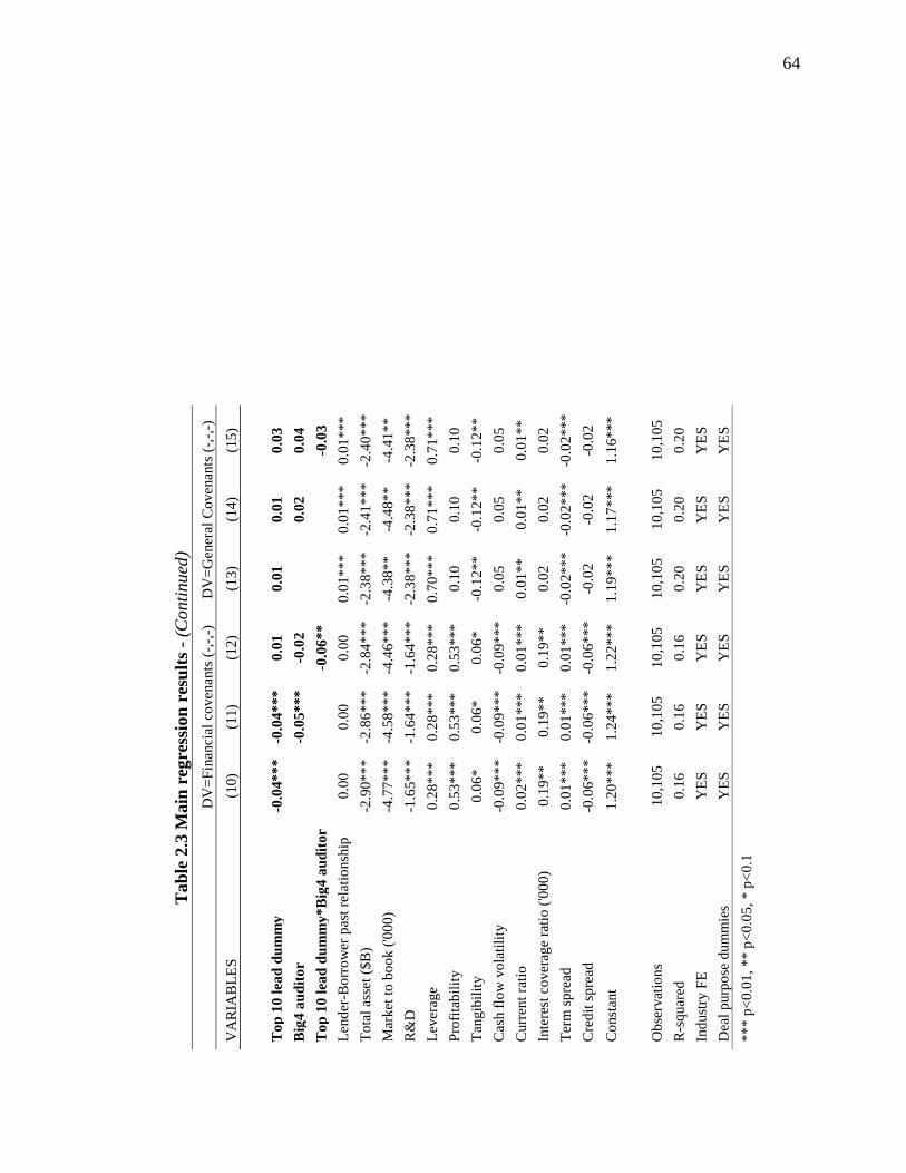
64
Tab
le 2
.3 M
ain
reg
ress
ion
res
ult
s -
(Conti
nued
)
D
V=
Fin
anci
al c
oven
ants
(-,
-,-)
D
V=
Gen
eral
Co
venan
ts (
-,-,
-)
VA
RIA
BL
ES
(1
0)
(11
) (1
2)
(13
) (1
4)
(15
)
To
p 1
0 l
ead
du
mm
y
-0.0
4*
**
-0.0
4*
**
0.0
1
0.0
1
0.0
1
0.0
3
Big
4 a
ud
ito
r
-0.0
5*
**
-0.0
2
0
.02
0.0
4
To
p 1
0 l
ead
du
mm
y*
Big
4 a
ud
ito
r
-0.0
6*
*
-0.0
3
Lend
er-B
orr
ow
er p
ast
rela
tio
nsh
ip
0.0
0
0.0
0
0.0
0
0.0
1***
0
.01
***
0
.01
***
To
tal
asse
t ($
B)
-2.9
0**
*
-2.8
6**
*
-2.8
4**
*
-2.3
8**
*
-2.4
1**
*
-2.4
0**
*
Mar
ket
to
bo
ok (
'00
0)
-4.7
7**
*
-4.5
8**
*
-4.4
6**
*
-4.3
8**
-4
.48
**
-4
.41
**
R&
D
-1.6
5**
*
-1.6
4**
*
-1.6
4**
*
-2.3
8**
*
-2.3
8**
*
-2.3
8**
*
Lever
age
0.2
8***
0
.28
***
0
.28
***
0
.70
***
0
.71
***
0
.71
***
Pro
fita
bil
ity
0
.53
***
0
.53
***
0
.53
***
0
.10
0.1
0
0.1
0
Tan
gib
ilit
y
0.0
6*
0.0
6*
0.0
6*
-0.1
2**
-0
.12
**
-0
.12
**
Cas
h f
low
vo
lati
lity
-0
.09
**
*
-0.0
9**
*
-0.0
9**
*
0.0
5
0.0
5
0.0
5
Curr
ent
rati
o
0.0
2***
0
.01
***
0
.01
***
0
.01
**
0
.01
**
0.0
1**
Inte
rest
co
ver
age
rati
o (
'00
0)
0.1
9**
0.1
9**
0.1
9**
0.0
2
0.0
2
0.0
2
Ter
m s
pre
ad
0.0
1***
0
.01
***
0
.01
***
-0
.02
**
*
-0.0
2**
*
-0.0
2**
*
Cre
dit
sp
read
-0
.06
**
*
-0.0
6**
*
-0.0
6**
*
-0.0
2
-0.0
2
-0.0
2
Co
nst
ant
1.2
0***
1
.24
***
1
.22
***
1
.19
***
1
.17
***
1
.16
***
Ob
serv
atio
ns
10
,105
10
,105
10
,105
10
,105
1
0,1
05
10
,105
R-s
quar
ed
0.1
6
0.1
6
0.1
6
0.2
0
0.2
0
0.2
0
Ind
ust
ry F
E
YE
S
YE
S
YE
S
YE
S
YE
S
YE
S
Dea
l p
urp
ose
du
mm
ies
YE
S
YE
S
YE
S
YE
S
YE
S
YE
S
**
* p
<0
.01
, ** p
<0
.05
, * p
<0
.1

65
In Table 2.4, we report results in non-logged units for the convenience of interpretation
since all dependent variables are in natural logarithm form. Column 3 represents results for
interaction term on loan spread. As shown below, an average borrower with a non-top 10 lead
arranger and a non-big 4 auditor pays about 141.59 bps over floating interest rate after
controlling for their other risk factors. However, changing from a non-top 10 lead arranger to a
top 10 lead arranger would reduce their interest cost by about 16.38 bps. Similarly, having a big
4 auditor would reduce interest cost by about 11.27 bps. Most importantly, having both a top 10
lead arranger and a big 4 auditor at the same time would reduce interest cost significantly by
about 37 bps. That is for an average loan of 350 million USD, annual interest cost of 1.3 million
USD will be saved.
Table 2.4 Summary of main results
Conditions (3)
Spread
(in bps)
(6)
Amount
(in $Mill)
(9)
Maturity
(in years)
(12)
Fin_Cov
(in numbers)
Top10=0; Big4=0 141.59 21.33 2.92 3.39
Top10=1; Big4=0 125.21 56.26 3.39 -
Top10=0; Big4=1 130.32 46.99 3.13 -
Top 10=1; Big4=1 104.58 142.59 3.90 3.19
2.4.2 Certification effect increases loan amounts
As for loan amount, a borrower with a non-top 10 lead arranger and a non-big 4 auditor
gets an average of 21.33 million USD from the syndication. However, as they switch from a non-
big 4 auditor to a big 4 auditor their loan amount increases to 46.99 million USD by more than
two times. If the borrower obtains the loan from a top 10 lead arranger loan amount increases
even more to 56.26 million USD due to the top 10 lead arranger’s reputation and resource
capacity. For a borrower who has both a big 4 auditor and a top 10 lead arranger will get even

66
larger loans of 142.59 million USD which increases average loan amount significantly by about
35 percent. We believe both a reputable external auditor and a dominant lead arranger alleviate
information asymmetry for the syndicate participants to signal the borrower’s credibility.
Therefore, thanks to the enhanced certification effect, it is easier to collect funds from other
participants and the average loan size increases materially by about 142.59 million USD.
2.4.3 Certification effect increases loan maturity
We find a positive impact of certification effect for loan maturity as well as reported in
Table 3 and Table 4. While for the borrower with a non-top 10 lead arranger and a non-big 4
auditor average loan maturity is 2.9 years, with a top 10 lead arranger it increases by about a half
year to 3.4 years materially. In column 8, the significantly positive coefficient of 0.11 indicates
that even for top 10 lead arrangers, big 4 external auditors have information value. Further, when
we take the interaction of the two terms, it is positively significant, while maintaining
significances of coefficients for the top 10 lead arranger and the big 4 auditor dummies. In fact,
after converting the parameter estimates to non-logarithm form in Table 4 column 9, loan
maturity extends by about a year when the borrower has both a top 10 lead arranger and a big 4
external auditor.
2.4.4 Certification effect decreases loan financial covenants
As for loan financial covenants, while the dominant lead arranger and the big 4
certification effects are significant in separate, they no longer hold with the interaction term.
However, in column 12, the interaction term is significantly negative, implying positive effect of
certification. In numerical term, having both the dominant lead arranger and the reputable
external auditor in average decreases financial covenant by about 0.2. Moreover, as for general
covenants, as shown in column 13-15 of Table 2.3, the certification effect neither from a

67
dominant lead arranger nor from a big 4 external auditor is significant even the sign of the
interaction term is negative. Overall, the results suggest that as compared to other loan terms,
covenants are not so easily negotiated.
2.5 Robustness tests
2.5.1 Alternative estimation method
In the baseline analysis, we did not consider plausible correlations among dependent
variables. However, in practice, loan terms are negotiated as a set. So do the Pearson’s
correlations in Table 2.2 Panel B indicate highly significant correlations among the dependent
variables. Depending on the loan amount, the interest rate could change due to economies of
scale impact. However, ignoring correlations among equations in the baseline analysis could
introduce significant bias to the results. Therefore, with an alternative estimation method to
allow correlations among dependent variables, we retest the model using seemingly unrelated
equation (SUR) following Zellner (1962).
The results from these analyses are represented in Table 2.5 Panel B and compared with
the baseline results in Panel A. Since only our assumption of error terms changes, parameter
estimates remain the same as in the baseline case and the statistical significances changes due to
changes in standard errors. As shown above, with SUR specification, economic significances of
the interaction term between the dominant lead arranger and the big 4 auditor improves for the
loan amount, maturity, and financial covenant. We conclude that with an alternative SUR
estimation method baseline results hold even stronger.

68
Table 2.5 Robustness test: comparison with SUR estimation method
Panel A: Baseline results
Spread Amount Maturity Fin_Cov Gen_cov
VARIABLES (3) (6) (9) (12) (15)
Top 10 lead dummy -0.13*** 0.97*** 0.15*** 0.01 0.03
Big4 auditor -0.09*** 0.79*** 0.07** -0.02 0.04
Top 10 lead dummy*Big4 auditor -0.09*** 0.14* 0.07** -0.06** -0.03
Control variables YES YES YES YES YES
Constant 4.96*** 3.06*** 6.97*** 1.22*** 1.16***
Panel B: SUR results
Spread Amount Maturity Fin_Cov Gen_cov
VARIABLES (3) (6) (9) (12) (15)
Top 10 lead dummy -0.13*** 0.97*** 0.15*** 0.01 0.03
Big4 auditor -0.09*** 0.79*** 0.07*** -0.02 0.04
Top 10 lead dummy*Big4 auditor -0.09*** 0.14** 0.07*** -0.06*** -0.03
Control variables YES YES YES YES YES
Constant 4.96*** 3.06*** 6.97*** 1.22*** 1.16***
2.5.2 Alternative measures for certification
We identify the dominant lead arranger based on its market share by its syndicated loan
volume as an alternative measure as compared to a number of transactions in case of baseline
analyses. The results hold with this alternative specification. In addition to that rather than Big 4
auditor dummy, we create a dummy for Big 6 auditors. In unreported analyses, results hold even
stronger.
2.6 Conclusion
Previous studies suggest certification role of reputed lenders with a positive impact on
borrower’s stock market returns. With evidence of syndicated loan, we test certification effect of
lead arranger’s reputation on loan price and non-price terms. Our results suggest information
value of reputable lead arrangers with significantly lower interest spread and the number of

69
financial covenants and increased loan amount and extended loan maturity. Moreover, we find
that external auditor could certify beyond that of lead arranger’s reputation by further adding
value to the borrower.

70
CHAPTER III:
DO PAST RELATIONSHIP AND EXPERIENCE HELP A BANK
IN WINNING A LEAD MANDATE IN THE SYNDICATED LOAN BID?
3.1 Introduction
In a traditional sole lender loan, a lender assesses the borrower, negotiates loan terms
with the borrower and monitors the loan. The lender must absorb all the credit risk in addition to
that receiving all income, it must bear all the losses. Unlike sole lender loans, a syndicated loan
involves two or more lenders issuing a loan to a common borrower under the same contract.
Thus, a syndicated loan has an advantage of risk-sharing among partners and alleviates loss
amount in case of credit defaults (Dennis and Mullineaux (2000)). With the emergence of global
companies and demand for large-scale loans, the syndicated loan market has grown substantially.
The U.S. market alone has multiplied about 6.4 times since 1989 to reach $1.36 trillion in 2013
(Board of Governors of the Federal Reserve System (2014)). The rapid growth of the market
with multi-dimensional principal-agent scenarios has drawn the attention of researchers to
explore behaviors of different players and their characteristics.
Many studies have been devoted to finding determinants alleviating information
asymmetry among syndicate parties. Borrower’s transparency (Ackert, Huang and Ramírez
2007)), credit rating (Sufi 2007), ownership structure (Lin, Ma, Malatesta and Xuan (2012)),
bankruptcy status (Gopalan, Nanda and Yerramilli (2011)), profitability and repeat lending
relationship (Bharath, Dahiya, Saunders and Srinivasan (2009), Farinha and Santos (2002),
Gangopadhyay and Mukhopadhyay (2002)) signal borrower’s creditworthiness, thus reducing
information asymmetry. For lender-lender relationship Ross (2010) emphasizes the significance
of lead bank reputation, Champagne and Kryzanowski (2007) and Cai (2009) explore previous

71
partnering relationships, role-switching, and free-riding incentives. Others have studied various
loan terms (Ackert, Huang and Ramírez (2007), Bharath, Dahiya, Saunders and Srinivasan
(2009)) and different business cycles (Anil and Wei-Ling (2011)).
As noted above a growing number of studies investigates syndicated loan structure and
highlights the importance of lead arrangers’ role. A borrower may select a lead arranger either
based on its previous relationship or through a competitive bid that requires high standard
qualification. Lead arrangers are in charge of originating, structuring, pricing, arranging and
underwriting the deal. Therefore, they should understand both borrower and other lender
requirements to clear the market, which requires great knowledge and expertise (Miller (2014)).
Consequently, it is common to have more than one lead arrangers in the deal to share
underwriting and syndicating responsibilities. As a reward for a lead mandate lead arrangers
obtain privileged access to the borrower’s private information, opportunities to build a
relationship, develop other non-credit business services, gain expertise and most importantly,
earn a lucrative share from the loan payoffs (Panyagometh and Roberts (2010)).
Campbell and Weaver (2013) divide loan syndication process into different phases,
namely pre-mandate, post-mandate and post contract signing phases. The focus of this study is
on the pre-mandate phase when the borrower invites a selected number of banks to bid for the
syndicated loan lead mandate and subsequently grants the mandate. While the borrower sets up
technical requirements for the potential lead arranger, bidders can participate either for a sole-
mandate or multi-bank group mandate for lead arrangers. In practice, borrowers decide which
option they want. Also, it is common that borrowers would restrict the bid to a sole lead
arrangement as it encourages a competitive environment that increases the borrower’s
negotiating power. For the purpose of this study we restrict the sample to sole-mandate deals

72
only, as an inclusion of deals with multi-bank group mandates would complicate the issue. This
is because multi-bank bidding is a separate game that involves various strategies between and
within bank groups as well as with the borrower, making empirical tests for identifying the
different practices difficult, if not altogether infeasible.
In practice, lenders are ranked by a league table which evaluates lender’s capability by
various criteria to meet the deal specific needs. This table distinguishes leading banks from those
that play less active roles. Moreover, a league table can be sector specific to identify leading
banks in that sector. Accordingly, a league table can be a sound first judgment to select potential
lead banks. Therefore, making it to the league table grants banks a competitive edge, access to
large competent clients and a partnership opportunity with other leading banks. However, only a
very limited number of lenders possess such resources and capacities. Campbell and Weaver
(2013) note that the majority of syndicated loan market players participate as investors only,
realizing partial benefits without a lead mandate.
So, what contributes to a lender winning a lead mandate in a potential loan syndicate? Is
it the financial strength of a bank that signals its syndicating capabilities when granting a
mandate? Or is it the bank’ past relationship with the borrower that grants a bank a competitive
advantage? Or is the bank’s experience or the specialization that matters? Although anecdotal
evidence suggests they all matter, there is no quantifiable evidence to support the argument.
Against that backdrop, the purpose of the paper is to address this gap in the research by
answering these questions with a focus on banking institutions since banks constitute the
majority, about 80 percent, of the syndicated loan market share (Board of Governors of the
Federal Reserve System (2014)). This is done on the basis of manual matching of bank Call

73
reports with syndicated loan (Dealscan) data, the method of study which facilitates the
examination of various bank characteristics and other behavioral variables.
Utilizing Logit regression, we find that financially strong banks are chosen as lead banks
in the syndicated loan to commit greater responsibilities. Moreover, behavioral variables such as
dominance in the market, previous relationship with the borrower and the expertise in the
borrower’s industry are both statistically and economically significant determinants of banks’
roles in the syndicate after controlling for financial variables. With an increase in the industry
experience ratio by 1 unit, the odds of winning a lead mandate increases by 47 percent.
Moreover, a one standard deviation increase in borrower industry experience increases the odds
of becoming a lead arranger by 5 percent. Also, as the past relationship with the borrower
increases by one standard deviation, it leads to 7 percent increase in odds for becoming a lead
arranger. Furthermore, for a top 10 player odds to become a lead arranger increases by percent
10 percent with one standard deviation change. Overall these results support the importance of
league table status, industry specialization and private knowledge.
Moreover, further analysis shows that the results are mainly driven by the pre-crisis
period subsample, implying that sole-mandate bids are common practice in good times when
funding is abundant. Also, these results hold true and even stronger for above median Tier 1
capital and above median total asset groups banks, considered to be solid candidates for lead
arranger when borrowers send bidding invitations. More specifically, for capital abundant
candidates it is the industry experience that matters most, as evidenced by a likelihood ratio of
1.97, compared to 1.47 in the baseline regression for all candidates. Similarly, the odds ratio for
having a previous relationship with the borrower and dominance in the market as indicated by a
top 10 lender dummy increased from 1.34 to 1.56 percent and from 1.21 to 1.31 respectively.

74
Similar, yet weaker results hold true for above median total asset group which indicates Tier 1
capital ratio and the total assets to be distinct measures of bank capacity. However, when we use
the number of transactions as alternative measures to the volume of transactions won for
measuring behavioral variables, the foregoing result holds for the top 10 bank dummy variable
only, indicating that borrowers appear to take quality more seriously than mere quantity.
The paper is organized as follows: Section 3.2 describes literature and hypotheses
development; Section 3.3 describes data and variables used in this study; Section 3.4 describes
the research methodology, Section 3.5 provides main results and discussions; Section 3.6
explains robustness tests and Section 3.7 concludes.
3.2 Literature and hypotheses development
3.2.1 Financial strength hypothesis
According to Shared National Credit Program of Federal Reserve System, a large
syndicated loan is defined as a loan of over $20 million that is shared by more than three
supervised institutions (Board of Governors of the Federal Reserve System (2014)). Playing a
crucial role of a lead arranger on a large scale and complex syndicated loan requires resources
and stronger capacity. Altunbaş and Kara (2011) highlight the presence of significant differences
between lead and participant banks in terms of their financial strength. More specifically they
observe lead banks to be larger in asset size, possess higher liquidity, profitability measured by
ROE and higher non-interest income while having lower capital ratios. They emphasize that
while participant banks lack resources to originate and arrange the deal, they enter into the
syndicate to diversify and boost income margin. Similar evidence has been found in Chu, Zhang

75
and Zhao (2014) in their study of lead and participant financial variables. Based on the above
argument we hypothesize that:
H3.1: Lead lenders possess stronger financial capacity than other lenders in the syndicate in
order to fulfill multi-functional responsibilities.
3.2.2 Hypotheses on past behaviors
League player: Lead arrangers must have superior capacity to screen the borrower, structure
deals, monitor the borrower and resolve any disputes. It is particularly true for project finance
deals that are considered the most demanding in terms of lead arrangers’ duties. While
prestigious lead arrangers provide high-quality service to both borrower and other participants, at
the same time they charge lower fees (Gatti, Kleimeier, Megginson and Steffanoni (2013)).
Moreover, dominant players in the market through their reputation can attract other lenders to
participate in the syndicate easily (Dennis and Mullineaux (2000)). Gopalan, Nanda and
Yerramilli (2011) demonstrate the significance of lead bank reputation for attracting other
participants even after a borrower bankruptcy.
Specialization: Due to the complex nature and idiosyncratic needs of borrowers it is difficult for
lead banks to be generalists. Rather, the specialization hypothesis assumes that lenders specialize
in particular deals to gain a comparative advantage. François and Missonier-Piera (2007) support
the specialization hypothesis and argue that syndicate partners choose their roles in the syndicate
consistent with their expertise in the borrower-specific transactions.
Private knowledge: Campbell and Weaver (2013) highlight the importance of previous
relationship and expertise in granting lead arranger mandates. Borrowers seek loans from the
banks they had relationships with in the past. Choosing the same lender not only reduces
transaction costs (Bharath, Dahiya, Saunders and Srinivasan (2009)) but also signals other

76
lenders about a borrower’s qualification (Farinha and Santos (2002), Gangopadhyay and
Mukhopadhyay (2002)). If the borrower approaches a new lender for a loan, the lender may
question the potential “lemon quality” of the borrower since the borrower had the option to
request the loan from its previous lenders. Lin, Ma, Malatesta and Xuan (2012) argue that
previous relationship with the borrower alleviates information asymmetry and find the
significant impact on syndicate formation. Furthermore, Champagne and Kryzanowski (2007)
emphasize the significance of long lasting relationships.
Therefore, based on the above arguments, we hypothesize the following:
H3.2: Lender’s past behaviors measured by dominance in the market (a proxy for league table
player), past borrower industry experience (a proxy for specialization), and the relationship with
the borrower (a proxy for private knowledge) are significant determinants of its role in the
syndicated loan
3.3 Data and variables
3.3.1 Sample construction
We use Thomson Reuter’s Dealscan database for dependent and loan related variables.
For bank financial information we manually match lenders from Dealscan with Bank Regulatory
call reports from Wharton WRDS by lender name and location as Dealscan reports banks by
their name and location only. Next, based on the Dealscan-Compustat link provided by Chava
and Roberts (2008) we construct bank behavioral variables. All our analysis is conducted at the
bank level and comprised of 47,479 bank-facility-year quarter observations for 13,029 unique
facilities over a period of time from the first quarter of 1996 to the third quarter of 2012.

77
3.3.2 Dependent variable
Dealscan, a global database for syndicated market, classifies lender roles as admin agent,
agent, co-agent, arranger, co-arranger, book-runner, collateral agent, custodian, documentation
agent, issuing agent, lead arranger, manager, mandated arranger, participant, senior co-arranger,
senior lead manager, senior manager, syndications agent and etc. The dependent variable is a
binary variable which takes a value of 1 if a bank is a lead arranger in the syndicated loan and 0
otherwise. We define banks as lead arrangers only if they are granted “Lead Arranger Credit”
status in the loan syndicate following Ertan (2015).
3.3.3 Bank behavioral variables
We include three different bank relationship and experience variables of banks following
Lin et al. (2012). The previous relationship between a bank and a specific borrower is measured
by the total USD deal amount issued to the same borrower within the past five years. The
stronger the previous relationship is, the less information asymmetry exists for the banks, which
in turn triggers greater lender commitments and incentive to play lead roles.
Bank experience is measured by industry expertise and dominance in the syndicated loan
market. Particularly we evaluate the actual dollar amount of deals that the bank made in the
borrower industry within the previous five years. We create a top ten bank dummy if a bank is
one of the top ten lenders in the syndicated loan market in terms of deal amount. We use
alternative measures for the above behavioral variables in terms of the number of deals and they
show high collinearity with the volume of deals. Moreover, the Logit outcomes show similar
results as those measured by the amount of deals so we use the ones measured by the deal
amount and report the results accordingly.

78
3.3.4 Bank financial variables
We believe bank financial variables demonstrate its business capacity and the ability of
greater commitments. Therefore, it is crucial to study their impact on the bank’s role in the
syndicated loan. Omitting these variables would cause potential endogeneity bias, so we control
for various variables. We take lagged values of these variables because both borrowers and
syndicate partners evaluate potential lead banks by past performance. In addition, this mitigates
reverse-causality.
We measure lender size by assets in millions of USD. Big banks with a large amount of
assets have the capacity to issue bigger loans, thus do not necessarily require another bank to
form a loan syndicate ceteris paribus. Therefore, lender size shall have a positive impact on
banks’ loan contribution as well as its choice of playing a lead arranger role. Moreover, we
control for the Tier 1 capital ratio of subject banks as it indicates funding capacity and ability to
absorb greater credit risks. We argue that high capital banks are more capable of issuing loans
without relying on costly outside funding. As a result, high capital banks should have a greater
propensity to play lead roles, all else being constant.
We control for risk-weighted asset share following Chu et al. (2014). The risk-weighted
asset is a proper measure of overall asset exposure weighted by their respective risk levels. It is
relevant for not only assessing risky asset amounts but also looks at the composition of
underlying asset portfolios. The higher the portion of high-risk assets in the total asset portfolio,
the more willingness a bank shall have for diversification. Moreover, we consider lender deposit
scaled by the total bank assets. Higher deposits outstanding indicate resource capacity, thus,
signaling less incentive to collaborate with others ceteris paribus. Liquidity is a measure for the

79
liquid asset resource to meet short-term liabilities, so large amounts of liquid assets imply greater
potential to issue sole-lender loans.
To control for bank profitability, we add ROA in the regressions. Higher ROA indicates
higher profitability. We argue that high-profit banks have more potential to issue loans by itself
and be in charge of greater commitments. Therefore, it shall have a positive impact on a bank’s
likelihood of becoming a lead arranger in the syndicate. Finally, loan allowance favors
borrowers, thus ceteris paribus, borrowers may prefer higher loan allowance rate banks over low
allowance rate banks to award a lead mandate.
3.3.5 Loan variables
We control for loan size as measured by the natural logarithm of the loan amount in
millions of US dollar. Large loans create bigger risks in case of borrower default thus, lenders
will choose to be participants to lower risks ceteris paribus. Moreover, we include loan maturity
in the analysis and take the natural logarithm of loan maturity measured in days. Loan maturity is
determined by the number of days between facility start date and facility end date. The long term
conveys higher a chance of variability, thus implying higher risk. By the same token, as risk
level increases banks participate rather than lead in order to diversify and alleviate risks.
We control for loan security as well. Because secured loan warrants payback, it reduces
loan risk significantly. As a result, banks are not as aggressive as in non-secured loans to reduce
risks and may prefer to retain a larger share of the loan for themselves and choose to play lead
arranger roles. Therefore, all else held constant we believe secured loans would have a positive
impact on the likelihood of becoming lead players.

80
In addition, we control for refinancing. Borrowers refinance for the purpose of seeking
more favorable terms in general. A new refinanced loan may benefit borrowers more in terms of
lower costs, longer maturity, fewer covenants and more relaxed conditions. Therefore, it may
increase risk exposure for lenders. As a result, we believe that loan refinancing makes banks less
likely to bid for lead arranger roles.
Last, we control for loan purpose. According to Dealscan, lenders cooperate in lending
for various reasons that include M&A, LBOs, takeover, recapitalization, debt repayment, and
working capital. Every purpose implies different risk exposure thus, we believe an inclusion of
the variable is relevant.
3.4 Methodology
We use a logistic regression model to study a bank’s propensity to be chosen as a lead
arranger in the syndicated loan. The dependent variable is a binary variable for a lead bank. We
include bank financial and behavioral variables along with loan terms which are crucial in
deciding to whom to grant mandates.
The empirical model is constructed as follow:
Lead bank𝑖,𝑗,𝑡 = 𝛽0 + 𝛾 ∗ 𝐵𝑎𝑛𝑘 𝑓𝑖𝑛𝑎𝑛𝑐𝑖𝑎𝑙 𝑣𝑎𝑟𝑖𝑎𝑏𝑙𝑒𝑠𝑖,𝑗,𝑡−1 + 𝛾 ∗
𝐵𝑎𝑛𝑘 𝑏𝑒ℎ𝑎𝑣𝑖𝑜𝑟𝑎𝑙 𝑣𝑎𝑟𝑖𝑎𝑏𝑙𝑒𝑠𝑖,𝑗,𝑡−1 + 𝛿 ∗ 𝐿𝑜𝑎𝑛 𝑣𝑎𝑟𝑖𝑎𝑏𝑙𝑒𝑠𝑖,𝑡 + 𝜗 ∗
𝐿𝑜𝑎𝑛 𝑝𝑢𝑟𝑝𝑜𝑠𝑒 𝑖𝑛𝑑𝑖𝑐𝑎𝑡𝑜𝑟𝑠𝑖,𝑡 + 𝜃 ∗ 𝐵𝑜𝑟𝑟𝑜𝑤𝑒𝑟 𝑖𝑛𝑑𝑢𝑠𝑡𝑟𝑦 𝑖𝑛𝑑𝑖𝑐𝑎𝑡𝑜𝑟𝑠𝑖,𝑡 + 𝜑 ∗
𝑄𝑢𝑎𝑟𝑡𝑒𝑟 𝑖𝑛𝑑𝑖𝑐𝑎𝑡𝑜𝑟𝑠𝑡 + 휀𝑖,𝑗,𝑡 𝑀𝑜𝑑𝑒𝑙 3.1
Lead, bank financial and behavioral variables are at loan-bank-year quarter level
frequencies and subscript i indicates loan, j indicates bank and t indicates a year-quarter. Loan

81
terms and loan purposes are defined uniquely for each loan. Also, we include borrower industry
and time fixed effects.
𝐿𝑒𝑎𝑑 𝑏𝑎𝑛𝑘 𝑖,𝑗,𝑡 is a dummy variable which takes a value of 1 if bank j is chosen as a lead
arranger in the syndicated loan i issued at t year-quarter. Bank financial variables measure
financial capacity including total assets, Tier 1 capital ratio, liquidity, profitability, risk-weighted
assets, deposits and loan allowance rates. Bank behavioral variables include past experience in
the borrower industry, past lending relationship with the borrower and the dominance in the
syndicated loan market. Both bank financial and behavioral variables are lagged under the
assumption that a lead mandate is granted based on the banks’ past performances. Loan variables
include different loan terms such as loan size, maturity, spread, collateral and refinancing
condition for loan i issued at time t.
Empirical tests for unobservable bidders for the lead mandate bring a challenge to the
analysis. Because of confidentiality of the borrower and competitive strategies of the banks, no
public information is available for sole mandate bidders. For the purpose of identifying the bid to
be sole-mandate, we restrict our sample to sole lead arranger deals regardless of the lender’s
banking status. In the case of club deals or multi-bank group bids, the book runner could be non-
bank institutions. Therefore, having only sole-lead syndicate loans shall exclude multi-bank
group bids, which is not the focus of this study.
With unobservable lead mandate bidders, conducting the tests for the complete sample
might introduce bias into the parameter estimates given that in such cases, all banks are treated
as potential bidders for the syndicate lead mandate. However, in practice, the borrower sends
invitations to bid to only a select number of banks that potentially could meet its requirements
and needs (Campbell and Weaver (2013)). Altunbaş and Kara (2011) find significant differences

82
in financial strength for lead arrangers consistent with their increased responsibilities in the loan
syndicate. Therefore, we follow a subsampling approach to address the unobservability problem.
We divide the sample into two groups based on total asset size and Tier 1 capital ratio as these
two variables signal the financial capacity of banks to fulfill lead arrangers’ greater
responsibilities. We expect that borrowers send invitations to bid to more highly qualified groups
possessing lower commitment risks. Therefore, more emphasis shall be given to above median
subsample groups.
3.5 Results and discussions
For a sample of 22,826 bank-loan-year quarter observations from the year 1996 to 1992,
15 percent of the banks are granted a lead mandate. Average bank size in the sample is 282.12
billion USD in assets with average Tier 1 capital ratio of 8.87 percent, well above regulatory
capital requirements. Risk-weighted assets, deposit, and loan allowance rates are measured as
percentages of bank’s total assets. Lender industry experience as a ratio of borrower’s industry
total volume of deals averages at 11 percent ranging from 4 to 14 percent at the 25th and 75th
percentiles, implying quite a diversified market structure.
Moreover, on average 25 percent of all loans of the borrower in the past 5 years are
funded by the same bank. Regarding dominant bank participation, 44 percent of the time, top 10
market players are involved in the syndicated loan. The average loan size is 353 million USD,
with a maturity of 48 months and spread of 173 bps over the floating rate. Finally, banks issue
loans to relatively secure borrowers with 63 percent of total loans being secured. Most of the
variables show significant correlations within an acceptable range.
Main results show that all the financial qualifications are crucial factors for a bank
playing a lead arranger’s role in the loan syndicate, thus supporting hypothesis 3.1.

83
Table 3.1 Descriptive statistics and Pearson’s correlations
The sample is collected over the first quarter of 1996 to the third quarter of 2012. The sample
involves 22,826 banks involving in 7,185 unique syndicated loan facilities with at least two
lenders and sole-lead arrangers. Panel A reports summary statistics of the data and Panel B
reports Pearson’s correlations among variables excluding dummy variables because correlation
matrix is not appropriate for the explanation of association with dummies. The bold figures
represent correlations that are significant at the 5 percent level. The variable descriptions are in
appendix A.
Panel A
N Mean Sd Median p25 p75
Bank variables
Lead 22,826 0.15 0.35 0.00 0.00 0.00
Lender size 22,826 282.12 428.84 77.76 37.39 268.95
Lender tier 1 capital ratio 22,826 8.87 3.20 8.21 7.56 9.30
Lender risk-weighted asset 22,826 83.67 15.39 82.44 73.26 91.61
Lender loan allowance rate 22,826 0.97 0.48 0.89 0.67 1.13
Lender ROA 22,826 0.70 0.57 0.63 0.34 1.00
Lender liquidity 22,826 21.56 10.17 20.07 15.13 25.64
Lender industry experience (ratio
to total lenders) 22,826 0.11 0.12 0.08 0.04 0.14
Past relationship with the
borrower (ratio to total lenders) 22,826 0.25 0.23 0.17 0.11 0.26
Top 10 lender (dummy indicator) 22,826 0.44 0.50 0.00 0.00 1.00
Loan variables
Loan maturity 22,826 48.21 21.15 59.80 36.50 60.87
Loan size 22,826 353.37 638.91 200.00 100.00 400.00
Loan spread 22,826 1.73 1.18 1.50 0.88 2.44
Loan security 22,826 0.63 0.48 1.00 0.00 1.00

84
Tab
le 3
.1 D
escr
ipti
ve
stati
stic
s an
d P
ears
on
’s c
orr
elati
on
s -
(Conti
nued
)
Pan
el B
: P
ears
on’s
corr
elat
ion
Var
iab
le n
am
es
[1]
[2]
[3]
[4]
[5]
[6]
[7]
[8]
[9]
[10
] [1
1]
[12
]
Lend
er s
ize
[1]
1
L
end
er t
ier
1 c
apit
al r
atio
[2
] -0
.24
1
Lend
er r
isk
-wei
ghte
d a
sset
[3
] -0
.22
-0
.27
1
L
end
er l
oan
all
ow
ance
rat
e [4
] -0
.1
0.0
4
0.1
9
1
Lend
er R
OA
[5
] -0
.03
-0
.12
0.1
8
0.0
3
1
L
end
er l
iquid
ity [
6]
-0.1
5
0.0
5
-0.3
3
-0.1
6
0.0
1
1
Lend
er i
nd
ust
ry e
xp
erie
nce
[7
] 0
.05
-0
.05
-0.0
1
0.0
1
0.0
2
-0.0
3
1
P
ast
rela
tio
nsh
ip w
ith t
he
bo
rro
wer
[8
] -0
.05
-0
.03
0
0.0
5
0
-0.0
2
0.1
1
1
Lo
an m
aturi
ty [
9]
0.0
2
0.0
1
-0.0
4
-0.0
7
0.0
1
-0.0
6
-0.0
3
-0.0
2
1
L
oan
siz
e [1
0]
0.0
5
0
0.0
2
-0.0
7
0
0
0.0
4
-0.0
4
0
1
Lo
an s
pre
ad [
11]
-0.0
2
0.1
-0
.03
0.1
7
-0.0
5
-0.0
2
-0.0
4
0.0
2
0.0
4
-0.4
2
1
L
oan
sec
uri
ty [
12
] -0
.03
0
.05
-0.0
2
0.0
8
-0.0
1
-0.0
7
-0.0
5
0.0
2
0.2
5
-0.3
4
0.5
5
1

85
Large size in terms of total assets increases a bank’s likelihood of becoming a lead
arranger in the syndicate as it could signal its capacity to fulfill multiple-tasks. The coefficient
for lender size is highly significant at the 1% level with an odds ratio of 1.86. Moreover, as
bank’s Tier 1 capital ratio increases by 1 percent, the odds of serving as lead arranger increases
by 5 percent, significant at 1% level. This result is consistent with previous evidence regarding
bank size and capitalization (Sufi (2007)).
However, the risk-weighted asset share adversely impacts bank becoming a lead arranger.
The result potentially implies that there is risk lowering incentives associated with already high-
risk portfolio banks. In addition to that, we find a significant negative impact with respect to
profitability (ROA), loan allowance rate and liquidity. Increased commitments of lead banks
particularly for fully underwritten deals may prevent bank management from aggressively
bidding for lead arranger mandates since it may adversely impact its future performance.
We argue that banks bid for the lead mandate if there is enough reward for its increased
commitments. Therefore, while for longer life and greater sized loans banks choose not to
aggressively bid for a lead mandate, as the loan prices increase or the loan becomes secured, they
tend to bid for the lead arranger’s mandate. The results hold for loan maturity, size and price
with the expected sign at a 1% level of significance.
Previous experience in the borrower’s industry as measured by the ratio of total volume
of deals in the past 5 years to all other lenders’ aggregate volume of deals is shown to be a
positive determinant of the likelihood of becoming a lead arranger in the syndicate at a 10% level
of significance. As the experience ratio increases by 1 unit, the odds of winning a lead mandate
increases by 47 percent. The result is economically significant too. A one standard deviation
increase in borrower industry experience increases the odds of becoming a lead arranger by 5

86
percent. Also, past relationship with the same borrower measured in terms of volume of deals
within past 5 years is crucial in winning a lead mandate.
Table 3.2 Main results
This table shows the baseline results for Logit model. The dependent variable is a lead bank
dummy which takes value of 1 for lead banks and 0 otherwise. Key independent variables are
past lender experience, previous relationship with the borrower and Top 10 dummy. Standard
errors are robust and clustered at loan facility. The ***, **, and * represent significance at the
1 percent, 5 percent, and 10 percent levels respectively.
VARIABLES Baseline Relationship & experience
Coefficient Odds Ratio e^bStdX
Lender size 0.66*** 0.62*** 1.86*** 2.85
Lender tier 1 capital ratio 0.05*** 0.05*** 1.05*** 1.18
Lender risk-weighted asset -0.02*** -0.02*** 0.98*** 0.75
Lender loan allowance rate -0.23*** -0.23*** 0.79*** 0.89
Lender ROA -0.22*** -0.21*** 0.81*** 0.89
Lender liquidity -0.02*** -0.02*** 0.98*** 0.84
Lender industry experience (ratio to
total lenders)
0.38** 1.47** 1.05
Past relationship with the borrower
(ratio to total lenders)
0.30*** 1.34*** 1.07
Top 10 lender (dummy indicator)
0.19*** 1.21*** 1.10
Loan maturity -0.19*** -0.19*** 0.83*** 0.89
Loan size -0.46*** -0.46*** 0.63*** 0.59
Loan spread -0.01 -0.01 0.99 0.99
Loan security 0.14*** 0.14*** 1.15*** 1.07
Observations 22,810 22,810
Time FE YES YES
Deal purpose dummies YES YES
Pseudo R2 0.196 0.198
Most importantly, as past relationship with the borrower increases by one standard
deviation, it leads to a 7 percent increase in the probability of becoming a lead arranger.
Furthermore, bank dominance in the syndicated market proxied by the top 10 dummy in terms of

87
volume of deals is a significant positive determinant of likelihood in receiving a lead mandate in
the prospective loan syndicate. The coefficient of 0.19 is not only statistically significant at the 5
percent level, but also the most significant behavioral factor in terms of its economic
significance.
Figure 3.1 Predictive margins for lead arrangers
More specifically, for a top 10 player, the odds of becoming a lead arranger increases by
10 percent with a one standard deviation change. Overall, these results support agency
hypotheses that past relationship and expertise alleviate information asymmetry thus, the

88
borrower grants the lead mandate to the bank it knows better to reduce lender commitment risks.
Therefore, we find support for hypotheses 3.2. Figure 1 demonstrates a positive relationship
between past behavioral variables and the propensity to be chosen as a lead arranger in the
syndicated loan. As lender industry experience, borrower relationship and the overall market
share increase it is more likely to be selected as lead banks in the syndicate.
Results are driven mainly due to pre-crisis period
Unlike multi-bank group bids, sole-lead mandate bids are attractive to borrowers in terms
of loan pricing as they encourage competitive bidding and prevent collusive behaviors. However,
when resources are scarce and credit flow is limited, sole-lead deals face greater commitment
risks. Therefore, including different business cycles could introduce bias to the parameter
estimates. Because the initial sample period includes the recent sub-prime mortgage crisis period
of 2008, we further split the sample into two groups. The Period before 2009 is considered the
pre-crisis period and the period after the post-crisis period. Indeed, 92 percent of all sole-lead
deals are signed during economic rest.
As shown in Table 3.3, results are mainly driven by the pre-crisis period. Parameter
estimates for behavioral variables become stronger both in terms of statistical and economic
significances. The odds ratio for lender industry experience increases from 1.47 to 1.68 with
improvement on economic significance from 5 percent to 1 percent. Similarly, the odds ratio for
past borrower relationship increases from 1.34 to 1.41 while the top 10 lender dummy remains
significant with a slight decrease economically. Conversely, results from the post-crisis sample
lose both statistical and economic significances. Overall, these results indicate that the past
behaviors of banks matters in winning lead mandates in general, however with respect to sole-
lead mandates, this only holds during economic up cycles.

89
Table 3.3 Pre and post crisis periods
The purpose of this table is to show results are mainly driven from the Pre-crisis period. The
dependent variable is a lead bank dummy which takes value of 1 for lead banks and 0 otherwise.
Key independent variables are past lender experience, previous relationship with the borrower
and Top 10 dummy. Standard errors are robust and clustered at loan facility. OR abbreiviates
Odds Ratios from the regression and e^bStdX represents economic significances of parameter
estimates to one standard deviation change. The ***, **, and * represent significance at the 1
percent, 5 percent, and 10 percent levels respectively.
VARIABLES All sample Pre-crisis Post-crisis
OR OR e^bStdX OR e^bStdX
Lender size 1.86*** 1.98*** 3.10 1.81*** 2.87
Lender tier 1 capital ratio 1.05*** 1.07*** 1.22 0.97 0.91
Lender risk-weighted asset 0.98*** 0.98*** 0.68 0.98** 0.74
Lender loan allowance rate 0.79*** 1.32*** 1.11 0.90 0.91
Lender ROA 0.81*** 0.76*** 0.86 0.90 0.93
Lender liquidity 0.98*** 0.99*** 0.87 1.00 0.98
Lender industry experience (ratio
to total lenders) 1.47** 1.68*** 1.06 0.11* 0.80
Past relationship with the borrower
(ratio to total lenders) 1.34*** 1.41*** 1.08 0.79 0.95
Top 10 lender (dummy indicator) 1.21*** 1.18*** 1.09 1.23 1.11
Loan maturity 0.83*** 0.87*** 0.92 0.84 0.91
Loan size 0.63*** 0.64*** 0.60 0.63*** 0.58
Loan spread 0.99 1.03 1.03 0.99 0.99
Loan security 1.15*** 1.13** 1.06 1.16 1.07
Observations 22,810 21,061 1,692
Time FE YES YES YES
Deal purpose dummies YES YES YES
Pseudo R2 0.198 0.211 0.204
3.6 Robustness tests
3.6.1 Dealing with selection bias
So far we include all observations in the analysis, treating non-lead banks as if they had
bid for the lead arranger mandate while in reality they may not have. Normally borrowers send
invitations for bidding only to a select number of candidates whom they believe could fulfill the
lead arranger’s responsibilities successfully while representing a low risk of not ultimately

90
committing to the loan. Sending invitations to every lender would not only be costly but also
endanger the borrower’s confidentiality. Therefore, an inclusion of all lenders in the sample may
underestimate the impact of behavioral variables.
Because lead mandate bidders are unobservable, it is not straightforward to validate the
results. As such, we follow a more practical but still reasonable subsample approach. We argue
that because the lead arranger’s role requires greater commitments, the borrower shortlists
candidates with greater capacity and resources. Using bank total assets and Tier 1 capital ratios
as indicators of capacity and resources, we further split the data on the basis of above and below
median values. Based on the argument that only greater capacity and resourced banks receive
bidding invitations, more emphasis shall be given to results from the above median samples.
Table 3.4 reports results from the different sub-samples. For comparison purposes, in the
first column, we report results from the pre-crisis subsample. Results from the above median and
below median values follow, which are divided further into two columns, the odds ratios, and
values for economic significance. Both the above median Tier 1 capital and above median total
asset subsamples provide stronger results in terms of magnitude while the below median value
subsamples are insignificant. For capital abundant candidates, industry experience matters the
most with an odds ratio of 1.97, meaning that improving the experience in the borrower’s
industry by 100 percent, increases the odds of winning lead mandate by 97 percent. Similarly,
increasing the previous relationship with the borrower by 1 unit increases the odds of becoming
the lead arranger by 56 percent (as opposed to 34 percent for the whole sample).
Dominance in the market indicated by the top 10 lender dummy results in an s
improvement of 10 percent, from 1.21 to 1.31 for capital abundant candidates. As shown,
parallel improvements are recognized in terms of economic significance for all three variables.

91
Regarding the above median total asset group, the magnitude of industry experience and past
relationship with the borrower improve, as with the Tier 1 capital group. The change in
magnitude is slightly weaker, perhaps because the Tier 1 capital ratio and total assets indicators
measure different aspects of bank capacity.
The below median groups show weak significance for industry experience and past
relationship with the borrower. Overall, results imply that past behaviors as measured by
industry experience, prior relationship with the borrower and being a top 10 player increases a
bank’s likelihood of winning a lead mandate in sole-lead bids. Moreover, smaller banks as
measured by their below median total assets and Tier 1 capital, could win lead arranger’s
mandate either through specialization or building a relationship with the borrower.
3.6.2 Alternative measures for behavioral variables
In the baseline results, behavioral variables are measured in volume of syndicated loan
deals. However, bank industry experience, past relationship with the borrower and dominance in
the syndicated loan market can be measured in terms of the number of transactions as well. Table
3.5 reports the results for alternative measures of behavioral variables. While the top 10 lender
dummy in terms of the number of deals shows consistent results, industry experience and past
relationship with the borrower both lose significances and are characterized by opposite signs.
For borrowers that emphasize commitment risks most significantly, past achievements measured
in terms of the volume of deals appear to be more important than the number of deals. It seems
that in the syndicated loan market quality matters most, rather than quantity.

92
Table 3.4 Subsample analyses
The purpose of this table is to highlight results from Above median subsamples. Panel A reports results
from subsamples by Tier 1 capital ratio and Panel B reports results from subsamples by Total Asset
respectively. The dependent variable is a lead bank dummy which takes value of 1 for lead banks and 0
otherwise. Key independent variables are past lender experience, previous relationship with the borrower
and Top 10 dummy. Standard errors are robust and clustered at loan facility. OR abbreiviates Odds Ratios
from the regression and e^bStdX represents economic significances of parameter estimates to one
standard deviation change. The ***, **, and * represent significance at the 1 percent, 5 percent, and 10
percent levels respectively.
PANEL A
VARIABLES Pre-crisis baseline Above median cap Below median cap
OR OR e^bStdX OR e^bStdX
Lender industry experience (ratio
to total lenders) 1.47** 1.97** 1.08 1.60* 1.06
Past relationship with the
borrower (ratio to total lenders) 1.34*** 1.56*** 1.11 1.29* 1.06
Top 10 lender (dummy indicator) 1.21*** 1.31*** 1.13 0.98 0.99
Financial variables YES YES YES
Loan terms YES YES YES
Observations 22,810 9,729 11,318
Time FE YES YES YES
Deal purpose dummies YES YES YES
Pseudo R2 0.198 0.231 0.216
PANEL B
VARIABLES Pre-crisis Above median TA Below median TA
OR OR e^bStdX OR e^bStdX
Lender industry experience (ratio
to total lenders) 1.47** 1.64* 1.05 1.83* 1.08
Past relationship with the
borrower (ratio to total lenders) 1.34*** 1.48*** 1.09 1.23 1.05
Top 10 lender (dummy indicator) 1.21*** 1.17*** 1.08 1.22 1.09
Financial variables YES YES YES
Loan terms YES YES YES
Observations 22,810 10,201 10,623
Time FE YES YES YES
Deal purpose dummies YES YES YES
Pseudo R2 0.198 0.149 0.168

93
3.7 Conclusion
We explore different factors for banks in winning a lead mandate. Obtaining a lead arranger
mandate in a syndication benefits lenders in terms of increasing market share, gaining expertise,
expanding profitability from both interest and non-traditional fees and developing new business
with the borrower. However, due to multifaceted responsibilities of lead banks, only a few
qualify for lead arranger mandates. Moreover, some banks prefer to play passive roles in the
syndicated loan market for the purpose of lowering their risk exposures. Therefore, it is crucial to
study different predictors for a bank to be chosen as lead bank in the syndicate.
Our findings suggest that financially strong and healthy banks are more likely to become
lead banks in the syndicated loan due to the necessity to commit to greater relative
responsibilities. In addition, we find past behaviors such as dominance in the syndicated loan
market, previous relationship with the borrower and expertise in the borrower’s industry
increases a bank’s likelihood of winning a lead mandate beyond bank’s financial strength.
Moreover, further analysis shows that results are mainly driven by the pre-crisis period
subsample, implying sole-mandate bids are common practice in good times when funding is
abundant. Results hold and are even stronger for above median Tier 1 capital and total asset
groups. Finally, it appears that borrowers take quality more seriously than quantity when we use
number of transactions as alternative measures to volume of transactions.

94
Table 3.5 Behavioral variables as measured by the number of deals
This table shows the baseline results for Logit model. The dependent variable is a lead bank
dummy which takes value of 1 for lead banks and 0 otherwise. Key independent variables are
past lender experience, previous relationship with the borrower and Top 10 dummy. Standard
errors are robust and clustered at loan facility. The ***, **, and * represent significance at the 1
percent, 5 percent, and 10 percent levels respectively.
VARIABLES Baseline Relationship & experience
Coefficient Odds Ratio e^bStdX
Lender size 0.66*** 0.60*** 1.83*** 2.76
Lender tier 1 capital ratio 0.05*** 0.05*** 1.05*** 1.16
Lender risk-weighted asset -0.02*** -0.02*** 0.98*** 0.72
Lender loan allowance rate -0.23*** -0.22*** 0.80*** 0.90
Lender ROA -0.22*** -0.21*** 0.81*** 0.89
Lender liquidity -0.02*** -0.02*** 0.98*** 0.83
Lender industry experience (ratio to
total lenders)
-0.02 0.98 1.00
Past relationship with the borrower
(ratio to total lenders)
-0.02 0.98 1.00
Top 10 lender (dummy indicator)
0.29*** 1.34*** 1.16
Loan maturity -0.19*** -0.19*** 0.82*** 0.88
Loan size -0.46*** -0.46*** 0.63*** 0.58
Loan spread -0.01 -0.01 0.99 0.99
Loan security 0.14*** 0.14*** 1.15*** 1.07
Observations 22,810 22,810
Time FE YES YES
Deal purpose dummies YES YES
Pseudo R2 0.196 0.198

95
REFERENCES
Ackert, Lucy F., Rongbing Huang, and Gabriel G. Ramírez, 2007, Information opacity, credit
risk, and the design of loan contracts for private firms, Financial Markets, Institutions
and Instruments 16, 221-242.
Allen, Franklin, and Douglas Gale, 2000, Financial contagion, Journal of Political Economy
108, 1-33.
Altunbaş, Yener, and Alper Kara, 2011, Why do banks join loan syndications? The case of
participant banks, The Service Industries Journal 31, 1063-1074.
Anil, Shivdasani, and Song Wei-Ling, 2011, Breaking down the barriers: Competition, syndicate
structure, and underwriting incentives, Journal of Financial Economics 99, 581-600.
Bayazitova, Dinara, and Anil Shivdasani, 2012, Assessing TARP, Review of Financial Studies
25, 377-407.
Beatty, Randolph P, 1989, Auditor reputation and the pricing of initial public offerings,
Accounting Review 64, 693-709.
Beatty, Randolph P, and Jay R Ritter, 1986, Investment banking, reputation, and the
underpricing of initial public offerings, Journal of Financial Economics 15, 213-232.
Benmelech, Efraim, and Jennifer Dlugosz, 2010, The credit rating crisis, NBER Macroeconomics
Annual 2009 24, 161-208.
Berger, Allen N., and Raluca A. Roman, 2013, Did TARP recipients get a competitive
advantage? An empirical study on competition in banking, Working Paper, Federal
Deposit Insurance Corporation.
Bharath, Sreedhar, Sandeep Dahiya, Anthony Saunders, and Anand Srinivasan, 2007, So what do
I get? The bank's view of lending relationships, Journal of Financial Economics 85, 368-
419.
Bharath, Sreedhar T., Sandeep Dahiya, Anthony Saunders, and Anand Srinivasan, 2009, Lending
relationships and loan contract terms, Review of Financial Studies 24, 1141-1203.
Billett, Matthew T., Mark J. Flannery, and Jon A. Garfinkel, 1995, The effect of lender identity
on a borrowing firm's equity return, The Journal of Finance 50, 699-718.
Black, L.K., and L.N. Hazelwood, 2012 The effect of TARP on bank risk-taking, Journal of
Financial Stability 9, 790-803.

96
Board of Governors of the Federal Reserve System, FDIC, OCC, 2014, Shared National Credits
Program 2014 Review, Online report available at
https://www.federalreserve.gov/newsevents/press/bcreg/bcreg20141107a1.pdf
Brunnermeier, Markus K, 2009, Deciphering the liquidity and credit crunch 2007-08, Journal of
Economic Perspectives 23, 77-100.
Cadman, Brian, Mary Ellen Carter, and Luann J. Lynch, 2012, Executive compensation
restrictions: Do they restrict firms’ willingness to participate in TARP?, Journal of
Business Finance & Accounting 39, 997-1027.
Cai, Jian, 2009. Competition or collaboration? The reciprocity effect in loan syndication
Working Paper, Federal Reserve Bank of Cleveland.
Campbell, Mark, and Christoph Weaver, 2013. Syndicated lending practice and documentation,
6th ed, (Euromoney Institutional Investor, London, UK).
Carter, Richard, and Steven Manaster, 1990, Initial public offerings and underwriter reputation,
The Journal of Finance 45, 1045-1067.
Champagne, Claudia, and Lawrence Kryzanowski, 2007, Are current syndicated loan alliances
related to past alliances?, Journal of Banking and Finance 31, 3145-3161.
Chari, Varadarajan Venkata, and Ravi Jagannathan, 1988, Banking panics, information, and
rational expectations equilibrium, The Journal of Finance 43, 749-761.
Chava, Sudheer, and Michael R. Roberts, 2008, How does financing impact investment? The
role of debt covenants, Journal of Finance 63, 2085-2121.
Chen-Lung, Chin, Yao Wei-Ren, and Liu Pei-Yi, 2014, Industry audit experts and ownership
structure in the syndicated loan market: At the firm and partner levels, Accounting
Horizons 28, 749-768.
Chen, Peter F., Shaohua He, Zhiming Ma, and Derrald Stice, 2015, The information role of audit
opinions in debt contracting, Journal of Accounting and Economics 61, 121-144.
Chu, Yongqiang, Donghang Zhang, and Yijia Zhao, 2014, Bank capital and lending: Evidence
from syndicated loans, Working Paper, University of South Carolina.
Coleman, Anthony D. F., Neil Esho, and Ian G. Sharpe, 2006, Does bank monitoring influence
loan contract terms?, Journal of Financial Services Research 30, 177-198.
Cook, Douglas O., Carolin D. Schellhorn, and Lewis J. Spellman, 2003, Lender certification
premiums, Journal of Banking & Finance 27, 1561-1579.

97
Cornett, Marcia Millon, Lei Li, and Hassan Tehranian, 2013, The performance of banks around
the receipt and repayment of TARP funds: Over-achievers versus under-achievers,
Journal of Banking and Finance 37, 730-746.
Dennis, Steven A., and Donald J. Mullineaux, 2000, Syndicated loans, Journal of Financial
Intermediation 9, 404-426.
Diamond, Douglas W., and Philip H. Dybvig, 1983, Bank runs, deposit insurance, and liquidity,
Journal of Political Economy 91, 401-419.
Diamond, Douglas W., and Philip H. Dybvig, 1986, Banking theory, deposit insurance, and bank
regulation, The Journal of Business 59, 55-68.
Do, Viet, and Tram Vu, 2010, The effects of reputation and relationships on lead banks’
certification roles, Journal of International Financial Markets, Institutions and Money
20, 475-489.
Duchin, Ran, and Denis Sosyura, 2012 The politics of government investment, Journal of
Financial Economics 106, 24-48.
El Ghoul, Sadok, Omrane Guedhami, Jeffrey A. Pittman, and Sorin Rizeanu, 2015, Cross-
country evidence on the importance of auditor choice to corporate debt maturity,
Contemporary Accounting Research, Forthcoming.
Ertan, Aytekin, 2015, Real earnings management in the financial industry, Working paper,
London Business School.
Fang, Lily Hua, 2005, Investment bank reputation and the price and quality of underwriting
services, The Journal of Finance 60, 2729-2761.
Farinha, Luısa A., and João A. C. Santos, 2002, Switching from single to multiple bank lending
relationships: Determinants and implications, Journal of Financial Intermediation 11,
124-151.
Focarelli, Dario, Alberto Franco Pozzolo, and Luca Casolaro, 2008, The pricing effect of
certification on syndicated loans, Journal of Monetary Economics 55, 335-349.
Fortin, Steve, and Jeffrey A. Pittman, 2007, The role of auditor choice in debt pricing in private
firms, Contemporary Accounting Research 24, 859-896.
François, Pascal, and Franck Missonier-Piera, 2007, The agency structure of loan syndicates,
Financial Review 42, 227-245.

98
Gaby, Max, and David A. Walker, 2011, Impacts of TARP on financial institutions, Journal of
Applied Finance 21, 73-87.
Gangopadhyay, Shubhashis, and Bappaditya Mukhopadhyay, 2002, Multiple bank lending and
seniority in claims, Journal of Economics and Business 54, 7-30.
Gatti, Stefano, Stefanie Kleimeier, William Megginson, and Alessandro Steffanoni, 2013,
Arranger certification in project finance, Financial Management 42, 1-40.
Gilson, Stuart C, and Jerold B Warner, 1998, Private versus public debt: Evidence from firms
that replace bank loans with junk bonds, Working Paper, Harvard Business School,
Available at SSRN 140093.
Gopalan, Radhakrishnan, Vikram Nanda, and Vijay Yerramilli, 2011, Does poor performance
damage the reputation of financial intermediaries? Evidence from the loan syndication
market, The Journal of Finance 66, 2083-2120.
Gopalan, Radhakrishnan, Gregory F. Udell, and Vijay Yerramilli, 2011, Why do firms form new
banking relationships?, Journal of Financial and Quantitative Analysis 46, 1335-1365.
Gorton, Gary, 1985, Clearinghouses and the origin of central banking in the united states, The
Journal of Economic History 45, 277-283.
Harris, Oneil, Daniel Huerta, and Thanh Ngo, 2013, The impact of TARP on bank efficiency,
Journal of International Financial Markets, Institutions and Money 24, 85-104.
Heckman, James J, 1979, Sample selection bias as a specification error, Econometrica 47, 153-
162.
Hollowell, Byron J., 2011, Examining the long-term performance of TARP firms, Journal of the
Academy of Business and Economics 11, 162-177.
Huerta, Daniel, Daniel Perez-Liston, and Dave Jackson, 2011, The impact of TARP bailouts on
stock market volatility and investor fear, Banking and Finance Review 3, 45-54.
Ivashina, Victoria, 2005, The effects of syndicate structure on loan spreads, Working paper,
Stern Business School, New York University.
James, Christopher, 1987, Some evidence on the uniqueness of bank loans, Journal of Financial
Economics 19, 217-235.
Karjalainen, Jukka, 2011, Audit quality and cost of debt capital for private firms: Evidence from
Finland, International Journal of Auditing 15, 88-108.

99
Kim, Dong H., and Duane Stock, 2012, Impact of the TARP financing choice on existing
preferred stock, Journal of Corporate Finance 18, 1121-1142.
Kim, Jeong-Bon, and Byron Y. Song, 2011, Auditor quality and loan syndicate structure,
Auditing: A Journal of Practice and Theory 30, 71-99.
Kim, Jeong-Bon, ByronYang Song, and Judy S. L. Tsui, 2013, Auditor size, tenure, and bank
loan pricing, Review of Quantitative Finance and Accounting 40, 75-99.
Kodres, Laura E., and Matthew Pritsker, 2002, A rational expectations model of financial
contagion, The Journal of Finance 57, 769-799.
Lee, Sang Whi, and Donald J Mullineaux, 2004, Monitoring, financial distress, and the structure
of commercial lending syndicates, Financial Management 33, 107-130.
Li, Lei, 2013, TARP funds distribution and bank loan supply, Journal of Banking and Finance
37, 4777-4792.
Lin, Chen, Yue Ma, Paul Malatesta, and Yuhai Xuan, 2012, Corporate ownership structure and
bank loan syndicate structure, Journal of Financial Economics 104, 1-22.
Lummer, Scott L., and John J. McConnell, 1989, Further evidence on the bank lending process
and the capital-market response to bank loan agreements, Journal of Financial
Economics 25, 99-122.
Mariassunta, Giannetti, and Laeven Luc, 2012, The flight home effect: Evidence from the
syndicated loan market during financial crises, Journal of Financial Economics 104, 23-
43.
McCahery, Joseph, and Armin Schwienbacher, 2010, Bank reputation in the private debt market,
Journal of Corporate Finance 16, 498-515.
Miller, Steven, 2014, Lcd’s loan market primer (Standard and Poor’s Financial Services LLC).
Pagano, Marco, and Paolo Volpin, 2010, Credit ratings failures and policy options, Economic
Policy 25, 401-431.
Panyagometh, Kamphol, and Gordon S. Roberts, 2010, Do lead banks exploit syndicate
participants? Evidence from ex post risk, Financial Management 39, 273-299.
Ross, David Gaddis, 2010, The “dominant bank effect:” How high lender reputation affects the
information content and terms of bank loans, Review of Financial Studies 23, 2730-2756.

100
Santos, João A.C., 2001, Bank capital regulation in contemporary banking theory: A review of
the literature, Financial Markets, Institutions and Instruments 10, 41-84.
Slovin, Myron B., Marie E. Sushka, and Carl D. Hudson, 1990, External monitoring and its
effect on seasoned common stock issues, Journal of Accounting and Economics 12, 397-
417.
Sufi, Amir, 2007, Information asymmetry and financing arrangements: Evidence from
syndicated loans, The Journal of Finance 62, 629-668.
Taliaferro, Ryan, 2009, How do banks use bailout money? Optimal capital structure, new equity,
and the TARP, Working Paper, Harvard Business School.
Titman, Sheridan, and Brett Trueman, 1986, Information quality and the valuation of new issues,
Journal of Accounting and Economics 8, 159-172.
Treasury, U.S. Department of, 2013, Capital purchase program report, Online report available at
https://www.treasury.gov/initiatives/financial-stability/TARP-Programs/bank-investment-
programs/cap/Pages/default.aspx.
Wooldridge, J. M., 2002, Econometric analysis of cross section and panel data (Cambridge,
MA: MIT Press).
Yildirim, Sinan, and Kalpana Pai, 2012, Stock market volatility of the financial industry after
TARP, Journal of Applied Financial Research 2, 61-68.
Zellner, Arnold, 1962, An efficient method of estimating seemingly unrelated regressions and
tests for aggregation bias, Journal of the American Statistical Association 57, 348-368.

101
APPENDIX
VARIABLE DEFINITION
Panel A. Variables common to Chapters II-IV
Variable name Variable definition
Bank characteristics (Source: Bank Call Reports)
Size
Natural log of total assets in USD millions and the mean of bank’s
assets if there are more than one banks in a package: bhck2170 or
rcfd2170
Tier 1 capital ratio
Tier-I capital ratio and the mean of bank’s Tier-I capital ratios if there
are more than one banks in a package: bhck8274/bhcka223 or
rcfd8274/rcfda223
Risk-weighted assets
Risk-weighted assets/total assets ratio and the mean of the ratios if there
are more than one banks in a package: bhcka223/bhck2170 or
rcfda223/rcfd2170
Deposits
Deposits to total assets ratio and the mean of the ratios if there are more
than one banks in a package: (bhdm6631+ bhdm6636+ bhfn6631+
bhfn6636)/bhck2170 or rcfd2200/rcfd2170
Cash (B$) Cash/total assets ratio and the mean of the ratios if there are more than
one banks in a package: bhck0010/bhck2170 or rcfd0010/rcfd2170
Loan allowance rate
Loan allowance/total assets ratio and the average of the ratios if there
are more than one banks in a package: bhck3123/bhck2170 or
rcfd3123/rcfd2170
Charge off rate
Loan charge off/total assets ratio and the mean of the ratios if there are
more than one banks in a package: bhck4635/bhck2170 or
riad4635/rcfd2170
ROA Net income/total assets ratio and the mean of the ratios if there are more
than one banks in a package: bhck4340/bhck2170 or riad4340/rcfd2170
Liquidity
(Cash+available for sale securities)/total assets ratio and the mean of the
ratios if there are more than one banks in a package:
(bhck0010+bhck1773)/bhck2170 or (rcfd0010+rcfd1773)/rcfd2170
Leverage ratio Tier 1 capital/total assets and the mean of the ratios if there are more
than one banks: bhck8274/bhck2170 or riad8274/rcfd2170
Total lender industry
experience
(number/volume of
deals)
Sum of bank's industry experience ratios. The industry experience is a
ratio of bank’s total number (volume) of deals in a borrower’s 3-digit
SIC -code industry in the past five years divided by the total number
(volume) of deals in the same industry in the past five years
Total lender-borrower
past relationship
(number/volume of
deals)
Sum of bank’s past relationship ratios. The past relationship equals total
number (volume) of deals with the same borrower in the past five years
divided by the total number (volume) of deals of the borrower with all
banks in the past five years
Total number of top
10 lead lenders
Sum of top-10 banks in the package. The top-10 bank takes value of 1 if
the bank ranks in the top ten banks in terms of total number/volume of
deals in USD billions it has issued in the past 5 years and 0 otherwise

102
APPENDIX (Continued)
Panel A. Variables common to Chapters II-IV
Variable name Variable definition
Borrower characteristics (Source: Compustat)
S&P Rating Existence of long-term SP credit rating for the borrower in the previous
quarter, it equals to one if the borrower is rated and zero otherwise
Tobin’s Q
Market Value of Total Assets divided by the book Value of Total Assets
where the market Value of Total Assets is: (cshoq*prccq+atq-ceqq-
txdbq)/atq and txdbq is replaced by zero if missing ,following Chu et al.
(2014)
Market to book A ratio of market value of total equity to book value of total equity
(mkvaltq/ ceqq).
R&D rate
Borrower’s research and development expense divided by the book
value of total assets: xrdq/atq and xrdq are replaced by zero if missing
following Chu et al. (2014)
Leverage A ratio of debt to the total assets ((dlttq+ dlcq)/atq).
Profitability A ratio of operating income before depreciation to the total assets
(oibdpy/atq).
Cash holding Cash divided by the book value of total assets: cheq/atq
Size The ratio of plant, property and equipment to the total assets (ppentq/
atq).
Tangibility Net property, plant and equipment divided by total assets: ppentq/ atq
Cash flow volatility
Standard deviation of previous four quarters’ cash flows where cash
flow is (ibq+dpq)/saleq and dpq is replaced by zero if missing following
Chu et al. (2014)
Current ratio A ratio of current asset to current liability (actq/lctq).
Interest coverage ratio Natural logarithm of 1 plus interest coverage ratio (oiadpq/xintq).
Loan characteristics (Source: Dealscan)
Spread Loan spread over floating reference rate (allindrawn).
Loan maturity
Natural logarithm of facility maturity in days (facilityenddate-
facilitystartdate). Maturity at the package level is calculated as the
difference between the latest facility end date and the earliest facility
start date.
Loan size Natural logarithm of facility amount in millions of USD
(facilityamt*exchangerate/1,000,000).
Loan security
Dummy equal to one if loan is secured and zero otherwise. If at least
one facility of a package is secured, the package is considered secured
and is replaced by zero if missing
Loan purpose
dummies
Loan purpose dummy is coded as follows: 1=Corporate purpose, 2=
Working capital, 3=Takeover, 4=Debt repayment, 5=acquisition,
6=backup and 7=LBO, 8=Recapitalization and 9=others
Loan refinancing Dummy equal to one if loan is refinanced, and zero otherwise.

103
APPENDIX (Continued)
Panel B. Chapters II specific variables
Syndicate structure variables (Source: Dealscan)
Number of banks Number of banks participating in a syndicated loan
Number of lead banks Number of lead banks in a syndicated loan
Average bank loan
share
Bank loan share (in %) in a syndicate and mean of loan shares if there is
more than one banks. Missing values are replaced by 100% for
packages whose number of lenders equals one including non-bank
lenders.
Herfindahl index Sum of bank share squares in the syndicate. The value of Herfindahl
index ranges from 0 to 10,000.
TARP variables (Source: U.S. Treasury - CPP reports)
TARP loan dummy Takes the value of one if at least one lead bank in the syndicate is a
TARP recipient and zero if otherwise
TARP loan infusion
Mean of bank’s TARP infusion rates where TARP infusion is the total
TARP investment divided by the risk weighted assets and calculated if
the loan is issued while the bank is under the TARP program. For loans
with non-TARP recipients the value is equal to zero.
Political instrument variables (Source: Lei Li (2013))
Fed director Dummy which equals one if a bank's executive sat on the board of
directors of a Federal Reserve Bank (FRB) or a branch of a FRB
Democracy Dummy which equals 1 if a bank's local Representative was a Democrat
Subcomm. on FI
A Dummy which equals 1 if a bank's local Representative sat on the
Subcommittee on Financial Institutions and Consumer Credit in the
Financial Services Committee
Local Fire Donation
the percentage of campaign contributions from local fire industries in
total contributions received by a Representative in the 2007-2008
election cycle
Panel C. Chapters III specific variables
Loan covenants (Source: Dealscan)
Financial covenants
Natural log of the number of financial covenants. Financial covenants
include Max. Capex, Max. Debt to EBITDA, Max. Debt to Equity,
Max. Debt to Tangible Net Worth, Max. Leverage Ratio, Max. Loan to
Value, Max. Long-Term Investment to Net Worth, Max. Net Debt to
Assets, Max. Senior Debt to EBITDA, Max. Senior Leverage, Max.
Total Debt (including Cont.Liab) to Tangible Net Worth, Min. Cash
Interest Coverage, Min. Current Ratio, Min. Debt Service Coverage,
Min. EBITDA, Min. Equity to Asset Ratio, Min. Fixed Charge
Coverage, Min. Interest Coverage, Min. Net Worth to Total Asset, Min.
Quick Ratio, Other Ratio, Net Worth, and Tangible Net Worth.
General covenants
Natural log of the number of general covenants. General covenants
include Insurance Proceeds Sweep, Dividend Restriction, Equity
Issuance Sweep, Debt Issuance Sweep, Asset Sales Sweep, Excess Cash
Flow Sweep, % of Net Income, and % of Excess, Cash Flow.

104
APPENDIX (Continued)
Reputation variables (Source: Dealscan, Compustat)
Top 10 lead dummy
A binary variable that takes value of 1 if any of the lead arrangers in the
syndicated loan facility is one of the Top 10 lenders, Bank of America,
BNP Paribas, Citi, Credit Suisse, Deutsche Bank, GE Capital, JP
Morgan, Suntrust Bank, Wachovia and Wells Fargo, or 0 otherwise.
Big 4 auditor dummy
A binary variable that takes value of 1 if the borrower auditor (au) is
one of the Big four, PriceWaterHouse Coopers, Ernest & Young,
Deloitte & Touche and KPMG, or 0 otherwise.
Macro control variables (Source: Federal Reserve Bank)
Term spread
Following Kim et al. (2013), we take the difference of 10 year and 2
year U.S. Treasury bond rates one month before the facility becomes
active.
Credit spread
Following Kim et al. (2013), we take the difference of Baa and Aaa
rated U.S. corporate bond rates one month before the facility becomes
active.

105
VITA
BOLORTUYA ENKHTAIVAN
6620 N Bartlett Ave, Apt 2501
Laredo, TX 78041
956-220-6502
EDUCATION
Texas A&M International University Laredo, TX
Ph.D. in International Business (Major: Finance) May 2016
University of Virginia Charlottesville, VA
M.A in Economics December 2009
National University of Mongolia Ulaanbaatar, Mongolia
B.B.A in Finance June 2004
PROFESSIONAL CREDENTIAL
Candidate CFA level III exam June 2016
TEACHING EXPERIENCE
Texas A&M International University Laredo, TX
Risk Management Spring 2016
Managerial Economics Fall 2014, 2015
Business Statistics I Spring2014, 2015
Personal Finance Summer I 2014
International Business Summer II 2013
University of Virginia Charlottesville, VA
Seminar in principles of Microeconomics Fall 2010
WORK EXPERIENCE
Skytel LLC Ulaanbaatar, Mongolia
Director of Strategic Planning Department 2011
(Central) Bank of Mongolia Ulaanbaatar, Mongolia
Banking supervisor of Banking Supervision Division 2004-2008
CONSULTANT SERVICES
EPRC project under USAID Ulaanbaatar, Mongolia
Consultant on Loan Officers’ Training Program 2011
World Bank and Ministry of Finance of Mongolia Ulaanbaatar, Mongolia
Short Term Domestic Consultant 2004
Project on Improvement of Efficiency of Public Procurement under World Bank Assistance