three essays on empirical analysis of united states
TRANSCRIPT

i
The Pennsylvania State University
The Graduate School
The College of Earth and Mineral Sciences
THREE ESSAYS ON EMPIRICAL ANALYSIS OF
UNITED STATES ELECTRICITY MARKETS
A Dissertation in
Energy and Mineral Engineering
by
Suman Gautam
© 2014 Suman Gautam
Submitted in Partial Fulfillment
of the Requirements
for the Degree of
Doctor of Philosophy
December 2014

ii
The Dissertation of Suman Gautam was reviewed and approved* by the following:
Seth Blumsack
Associate Professor of Energy Policy and Economics
Dissertation Adviser
Chair of the Committee
Robert D. Weaver
Professor of Agriculture Economics
Jonathan P. Mathews
Associate Professor of Energy and Mineral Engineering
Zhen Lei
Assistant Professor of Energy and Environmental Economics
Luis F. Ayala H.
Associate Professor of Petroleum and Natural Gas Engineering
*Signatures are on file in the Graduate School

iii
Abstract:
In this Dissertation, three independent studies analyze the impact of recent changes in both
supply and demand sides of the U.S. electricity sector. Below is a brief description of three
essays.
I. Coal Plant’s Response to Renewable Portfolio Standards
Renewable Portfolio standards require load-serving entities to purchase a given percentage of
their electricity sales from eligible renewable energy technologies. This study analyzes the
impact of RPS on the coal utilization by coal plants of Pennsylvania, New Jersey, and Maryland
(PJM) electricity market. We develop a panel dataset of 259 unique PJM coal-fired utility plants’
integrating their fuel purchases with state-level RPS energy mandates, electricity prices, and fuel
prices from 2001 to 2011, covering both pre-RPS and post-RPS era. Since selection of RPS
policies may be non-random, we employ a two-step Heckit model to control for states’ decision
to adopt an RPS and choose yearly RPS levels. The results show that a percentage point increase
in state’s yearly energy target increases the average plant’s coal purchase by 45 thousand tons.
These results are approximately consistent across selection-corrected models. The analysis
showing the positive impact of RPS yearly targets on PJM coal plants’ coal purchases suggests a
few things. There are fewer coal plants operating at the margin. Moreover, RPS yearly energy
targets are fairly low at present; they are scheduled to increase considerably in coming years.
Renewable Portfolio Standards may decrease the amount of fuel utilized by coal plants when
RPS mandates increase in future.
II. Residential Customers Response to Critical Peak Events of Electricity: Green Mountain
Power Experience
Demand response (DR) programs, usually through peak pricing and incentive-based approaches,
can encourage customers to reduce or shift consumption during peak periods. This benefits
utilities by lowering short-run generation costs and reducing the need for some long-run peak-
driven investments. This paper analyzes the impact of Vermont’s Green Mountain Power’s
(GMP) emergency DR programs on residential customers’ electricity consumption during a two-
year pilot study program in 2012–2013. The 3,735 single-home residents of Central Vermont
area were separated into six treatment groups and two control groups resulting into 26 million
hourly load observations during the period of the study. Our analysis shows that incentive-based
demand response programs have statistically significant impacts on reducing peak load.
Specifically, CPR rates reduced peak load usage 6% to 7.7% and CPP rates reduced peak load
between 6.8% and 10.3% during critical peak events. Moreover, on average, IHD-equipped
participants’ monthly energy consumption was 2.0% to 5.3% lower than the monthly energy
usage of non-IHD customers. However, none of the CP rate and IHD treatments induced a
persistent response across multiple critical events and none of the treatment groups exhibited a
consistent response to critical peak events. Based on our evaluation of GMP’s DR programs
during 2012 and 2013, neither critical peak pricing nor rebates are themselves sufficient to
substitute for new capacity to meet resource adequacy requirements.

iv
III. Analysis of Load and Price patterns in the U.S. Electricity Sector
The study analyzes hourly electricity loads and marginal costs of electric entities with of extreme
value theory (EVT), a concept widely used in the financial sector. For each year’s hourly data of
balancing authorities and utilities, we fit generalized extreme value (GEV) distribution and
estimate the parameters of the distribution with an aim of comparing how these parameters have
changed over time and market regions. We also account for the time dependencies, seasonalities,
and near-time clustering present in the electricity markets – both for electricity load and prices –
with the help of autoregressive conditional hetereskedastic models. The results show that the
distributions of hourly load and lambda values are fat tailed. Hourly lambda values have more
extreme values generating fatter tails than hourly electricity load. We also show that extreme tail
quantiles estimated with the GEV parameters at different percentile levels are comparable with
the percentiles of actual observations.

v
Table of Contents
List of Figures …………………………………………………………………………………viii
List of Tables …………………………………………………………………………………....xi
Acknowledgements …………………………………………………………………………….xiv
Chapter 1: Introduction ............................................................................................................... 1
Chapter 2: Coal Plants’ Response to Renewable Portfolio Standards ........................................ 4
Introduction .......................................................................................................................... 5 1.
Background .......................................................................................................................... 8 2.
2.1 Coal-fired Power Plants ................................................................................................ 9
2.2 Fuel Procurement Methods ......................................................................................... 10
2.3 Renewable Portfolio Standards .................................................................................. 10
2.4 PJM Market ................................................................................................................ 12
Literature Review............................................................................................................... 14 3.
Theoretical model .............................................................................................................. 16 4.
Econometric Model ............................................................................................................ 20 5.
5.1 Base Model ................................................................................................................. 20
5.2 Addressing Selection Bias .......................................................................................... 22
Data .................................................................................................................................... 25 6.
6.1 Coal related variables ................................................................................................. 25
6.2 RPS data ..................................................................................................................... 25
6.3 Electricity and Fuel related variables ......................................................................... 26
6.4 Addressing Selection Problem: State-level data ......................................................... 26
Descriptive Statistics .......................................................................................................... 27 7.
Analysis and Results .......................................................................................................... 32 8.
8.1 Ordinary Least Square Estimation .............................................................................. 32
8.2 Addressing Selection Bias .......................................................................................... 34
8.3 Robustness Check – coal purchase/capacity as dependent variable ........................... 39
Conclusion ......................................................................................................................... 42 9.
References .......................................................................................................................... 45 10.
Appendix ............................................................................................................................ 48 11.
Chapter 3: Residential Customers Response to Critical Peak Events of Electricity: Green
Mountain Power Experience ......................................................................................................... 49
Introduction ........................................................................................................................ 50 1.

vi
Demand Response .............................................................................................................. 53 2.
2.1 Status of Demand Response programs in United States............................................. 54
Literature Review............................................................................................................... 57 3.
GMP Pilot Study ................................................................................................................ 59 4.
4.1 Participant Selection: Randomization, Eligibility, and Recruitment .......................... 61
4.2 Participants Characteristics ......................................................................................... 62
4.3 Critical Peak Events.................................................................................................... 66
4.4 Data ............................................................................................................................. 67
Theory ................................................................................................................................ 67 5.
5.1 Motivation .................................................................................................................. 67
5.2 Peak Load Change Analysis ....................................................................................... 71
5.3 Persistence Analysis ................................................................................................... 74
5.4 Energy Consumption Analysis ................................................................................... 75
Descriptive Statistics .......................................................................................................... 76 6.
Result and Analysis............................................................................................................ 86 7.
7.1 Peak Load Analysis .................................................................................................... 87
7.2 Persistence Analysis ................................................................................................... 90
7.3 Hourly Load Analysis of Transitioning Group ........................................................... 97
7.4 Energy Consumption Analysis ................................................................................... 99
Conclusion ....................................................................................................................... 101 8.
References ........................................................................................................................ 104 9.
Appendix .......................................................................................................................... 107 10.
Chapter 4: Analysis of Load and Price patterns in the U.S. Electricity Sector ...................... 112
Introduction ...................................................................................................................... 113 1.
Overview of United States Electricity Sector .................................................................. 116 2.
Extreme Value Theory and Implication in the Electricity Sector .................................... 119 3.
3.1 Block Maximum Method.......................................................................................... 122
3.2 Peaks-Over-Threshold Method ................................................................................. 125
3.3 Time Dependencies in Electricity Sector ................................................................. 128
Data Description and Tail Analysis ................................................................................. 132 4.
Empirical Analysis ........................................................................................................... 144 5.
5.1 Shape Parameters across Geographic Regions ......................................................... 147

vii
5.2 Estimating Tail Quantiles ......................................................................................... 151
Conclusion ....................................................................................................................... 156 6.
References ........................................................................................................................ 158 7.
Appendix .......................................................................................................................... 161 8.

viii
List of Figures
Figure 2-1: Average coal purchased by year ................................................................................ 29
Figure 2-2: Average coal purchased per MW by year .................................................................. 30
Figure 2-3: Quality of coal purchased and RPS yearly mandates ................................................ 31
Figure 2-4: Average fuel prices by year ....................................................................................... 31
Figure 2-5: Short-run electricity supply curve .............................................................................. 48
Figure 3-1: Timeline of the Green Mountain Power’s Study ....................................................... 60
Figure 3-2: Number of Rooms per Household ............................................................................. 63
Figure 3-3: Participants by household income .............................................................................. 65
Figure 3-4: Participants by Education Level ................................................................................ 65
Figure 3-5: Impact of single-fixed electricity price in welfare loss .............................................. 68
Figure 3-6: Impact of shift in electricity demand in wholesale electricity price .......................... 70
Figure 3-7: Average hourly load of IHD groups and no-notification control group during critical
peak events of 2012 ...................................................................................................................... 81
Figure 3-8: Average hourly load of no-IHD groups and no-notification control group during
critical peak events of 2012 .......................................................................................................... 82
Figure 3-9: Average hourly load of IHD groups and no-notification control group during critical
peak events of 2013 ...................................................................................................................... 83
Figure 3-10: Average hourly load of no-IHD groups and no-notification control group during
critical peak events of 2013 .......................................................................................................... 84

ix
Figure 3-11: Average monthly KW load for customers with and without in-home-display (IHD)
systems .......................................................................................................................................... 85
Figure 3-12: Average monthly KW load for customers by treatment group ................................ 86
Figure 3-13: Persistence Analysis – change in hourly electricity consumption (kW) – during
critical peak events of 2013 .......................................................................................................... 94
Figure 3-14: Daily load profile during Event days of 2012 for IHD groups .............................. 108
Figure 3-15: Daily load profile during Event days of 2012 for non-IHD groups ....................... 109
Figure 3-16: Daily load profile during Event days of 2013 for IHD groups .............................. 110
Figure 3-17: Daily load profile during Event days of 2013 for non-IHD groups ....................... 111
Figure 4-1: North American Electric Reliability regions (EIA, 2012b) ..................................... 118
Figure 4-2: Hourly load (GW) plot of PJM region from 2000 to 2012 ...................................... 120
Figure 4-3: Hourly lambda ($/MWh) of New York ISO from 2006 to 2012 ............................. 121
Figure 4-4: Types of extreme value distributions ....................................................................... 124
Figure 4-5: Time-series plot of residuals of PJM hourly load after using AR(1), AR(2), AR(24),
and GARCH(1,1) model during 2006 – 2012 ............................................................................. 131
Figure 4-6: Symmetry plot of hourly load (GW) observations of PJM region ........................... 141
Figure 4-7: Quantile plot of PJM’s hourly load against quantiles of Uniform distribution ....... 141
Figure 4-8: Quantile plot of PJM’s hourly load (GW) observations against Normal distribution
..................................................................................................................................................... 142
Figure 4-9: Symmetry plot of hourly lambda ($/MWh) observations of PJM region ................ 142

x
Figure 4-10: Quantile plot of PJM’s hourly lambda ($/MWh) against quantiles of Uniform
distribution .................................................................................................................................. 143
Figure 4-11: Quantile plot of PJM’s hourly lambda ($/MWh) observations against Normal
distribution .................................................................................................................................. 143
Figure 4-12: Flowchart of empirical analysis for estimating tail-quantiles of hourly load and
lambda values.............................................................................................................................. 146
Figure 4-13: Average annual load shape parameters for Electricity Providers. The electric entities
are available for all years during 2000 – 2012 period. ............................................................... 149
Figure 4-14: Average annual load shape parameters for Electricity Providers by Census regions.
The electric entities are available for all years during 2000 – 2012 period. ............................... 149
Figure 4-15: Average annual lambda shape parameter of Balancing Authorities. The electric
entities are available for all years during 2000 – 2012 period. ................................................... 150
Figure 4-16: Average annual lambda shape parameter of Balancing Authorities by Census
regions.The electric entities are available for all years during 2000 – 2012 period. .................. 150
Figure 4-17: Symmetry plot of hourly load (GW) observations of NYISO region .................... 161
Figure 4-18: Quantile plot of NYISO’s hourly load against quantiles of Uniform distribution . 161
Figure 4-19: Quantile plot of NYISO’s hourly load (GW) observations against Normal
distribution .................................................................................................................................. 162
Figure 4-20: Symmetry plot of hourly lambda ($/MWh) observations of NYISO region ......... 162
Figure 4-21: Quantile plot of NYISO’s hourly lambda ($/MWh) against quantiles of Uniform
distribution .................................................................................................................................. 163

xi
Figure 4-22: Quantile plot of NYISO’s hourly lambda ($/MWh) observations against Normal
distribution .................................................................................................................................. 163
Figure 4-23: Average annual load (GW) of Electricity Providers. The electric entities are
available for all years during 2000 – 2012 period. ..................................................................... 164
Figure 4-24: Average annual load (GW) of Electricity Providers by Census regions. The electric
entities are available for all years during 2000 – 2012 period. ................................................... 164
Figure 4-25: Average annual lambda ($/MWh) of balancing authorities. The electric entities are
available for all years during 2006 – 2012 period. ..................................................................... 165
Figure 4-26: Average annual lambda ($/MWh) of balancing authorities by Census regions. The
electric entities are available for all years during 2006 – 2012 period. ...................................... 165

xii
List of Tables
Table 2-1: Variable definitions, Means, and Standard Errors ...................................................... 28
Table 2-2: OLS results - Amount of Coal purchased ('000 tons) as dependent variable .............. 33
Table 2-3: Probit regression for RPS selection - RPS status as dependent variable ..................... 37
Table 2-4: Second stage results - linear prediction of RPS yearly targets .................................... 38
Table 2-5: OLS and Selection Corrected Results - Coal purchased ('000 tons) as dependent
variable .......................................................................................................................................... 39
Table 2-6: OLS results - Amount of coal purchased per name plate capacity ('000 ton/MW) as
dependent variable ........................................................................................................................ 41
Table 2-7: OLS and Selection Corrected results - Amount of coal purchased per nameplate
capacity ('000 ton/MW) as dependent variable ............................................................................. 42
Table 3-1: Required Sample sizes for the Study ........................................................................... 62
Table 3-2: Percentage of Household with different Appliances ................................................... 63
Table 3-3: Average temperature during five-hour of critical peak event hours ........................... 66
Table 3-4: Descriptive statistics, and summary of treatments, for the Year 1. ............................. 78
Table 3-5: Descriptive statistics, and summary of treatments, for the Year 2. ............................. 79
Table 3-6: Number of unique customers by group ....................................................................... 79
Table 3-7: Regression Results for Randomized Control Treatment Analysis .............................. 89
Table 3-8: Comparing coefficient estimates of CPP and CPP-IHD customers with RCT, RED,
and LATE methods ....................................................................................................................... 90

xiii
Table 3-9: Persistence Analysis: Within Event Hours .................................................................. 92
Table 3-10: Event-to-Event persistent analysis of year 2012 ....................................................... 93
Table 3-11: Persistence Analysis: year-to-year ............................................................................ 96
Table 3-12: Daily load analysis during event and non-event days ............................................... 97
Table 3-13: Hourly load analysis of transitioning treatment groups ............................................ 99
Table 3-14: Impact of IHD technology in monthly electricity usage (kW) ................................ 101
Table 3-15: Impact of IHD technology in daily electricity usage .............................................. 107
Table 3-16: Analysis for hours with Heat Index greater than 80 F -Year 2 ............................... 107
Table 4-1: Unique Electricity Providers by Census Regions for balanced panel of load results 136
Table 4-2: Unique Balancing Authorities by Census Regions for balanced panel of lambda
results .......................................................................................................................................... 136
Table 4-3: Detail descriptive statistics of hourly load (GW) electricity providers that are
available for most of the years during 2000 – 2012 period. ....................................................... 138
Table 4-4: Detail descriptive statistics of hourly load ($/MWh) electricity providers and
balancing authorities that are available for most of the years during 2000 – 2012 period. ........ 139
Table 4-5: Estimated hourly electricity load (GW) at 0.95 percentile ........................................ 153
Table 4-6: Estimated hourly electricity load (GW) at 0.99 percentile ........................................ 154
Table 4-7: Estimated hourly lambda ($/MWh) at 0.95 percentile .............................................. 155
Table 4-8: Estimated hourly lambda ($/MWh) at 0.99 percentile .............................................. 156

xiv
ACKNOWLEDGEMENTS
I would like to thank my PhD advisor, Professor Seth Blumsack, for supporting me
throughout my journey as a doctoral student. I appreciate his time, ideas, expertise, and funding
for completing my studies and dissertation research. I thank him for introducing me to the
exciting electricity markets research. I would also like to thank my dissertation committee
members, Professors R. D. Weaver, Jonathan Mathews, and Zhen Lei, for their continuous
support. Professor Weaver’s immense help improved the quality of my research. Professor
Mathews provided detailed comments on my dissertation and challenged me to think from a
different perspective. I equally appreciate Professor Lei’s support on improving the econometric
models in my study.
I will be forever thankful to my Master’s thesis advisor Dr. R. J. Briggs for patiently
sharing his research and programming skills during my first year in the Ph.D. program. Dr.
Briggs always challenged me to see research problems from a broader perspective. Similarly, I
am indebted to Professor Anastasia Shcherbakova for sharing a collaborating opportunity and
funding the second year of my graduate studies. I would like to thank Professor Andrew Kleit,
Energy Management and Policy Program Director, for accepting me to the doctoral program. My
appreciation also goes to Department of Energy and Mineral Engineering, Penn State University,
and its staff, Jamie Harter in particular. I would also like to thank the Energy Market Initiative,
Smart Grid Investment Grant, and U.S. Department of Energy for providing funding to complete
my Ph.D. education. I will be forever indebted to my undergraduate Physics Professors –
Narendra Jaggi and Gabe Spalding – for instilling in me a great research foundation and guiding
me to become an independent thinker.

xv
My four-year stay at Penn State would not have been enjoyable and fruitful without
support from many life-long friends. I appreciate the thoughtful discussions and quality time
spent with the friends in my department. Roger Mina, Anand Govindrajan, Yuxi Meng, Chen-
Hao Tsai, Xu Chen, Zhi Li, Mercedes Cortes, Babatunde Idrisu, Alisha Fernandez, Mostafa
Sahraei, Anukalp Narasimharaju, and Joohyun Cho are a few to name. Similarly, I was fortunate
enough to meet and spend time with the Nepalese students at Penn State. I will always remember
the time spent with and appreciate the support received from Madhav Kafle, Indira Pathak,
Krishna Roka, Punam Roka, Roshan Mainali, Sapana Mainali, Deepu Bhattarai, Nelly Bhattarai,
Saroj Adhikari, Naworaj Acharya, Sadikshya Adhikary, Sony Shrestha, Prakash Raj Timilsena,
Jwala Mani Adhikari, Sulav Paudel, Kabi Kafle, Samita Limbu, Moti Maya Gurung, Utsav
Pandey, Pasang Sherpa, Sanhrut Sapkota, Sastha Shrestha, Sandeep Regmi, and Punam Gurung.
I would like to thank my family and friends for their unconditional love, support, and
encouragement. My foremost gratitude goes to my parents, Arjun P. Gautam and Tara Gautam,
for their tireless effort in making sure that their children had better lives. I am fortune to have my
grandmother Ram Rekha Gautam’s blessing throughout my time away from home. I cannot
thank enough my younger sisters – Sabita, Sangita, Sachita, Prativa, Pratima, and brother Pratik
for their patience and support while I was away from home and not at their proximity when they
needed me. Their love aspired me to work continuously and diligently in my research. I also
appreciate the support from my other family members and relatives. Lastly, I sincerely
appreciate and thank my fiancée Sushmita Subedi for believing in me more than myself and
helping me to complete my dissertation.

1
Chapter 1: Introduction
The United States electricity sector has gone massive changes over the last few decades.
The deregulation of electricity in most of the US regions, new renewable energy policies and
subsidies, and implication of global warming has not only affected the demand and supply sides
of the electricity sector, but also raised the issue of the reliability and adequacy (Mansur, 2008;
Chandler, 2009; Lyon and Yin, 2010; FERC, 2012).
Some of the heavily affected areas with the new policies and market changes are coal-
fired power plants and utility sectors. The supply of coal-fired electricity has decreased 50% to
37% from 2002 to 20121 (EIA, 2013). Similarly, the increase in electricity demand during the
peak period has increased the reliability cost to the utilities (Spees, 2008; Faruqui et. al, 2010).
There is a need to develop rigorous mechanism in order to analyze the impact of the recent
changes by carefully acknowledging the specific details of each affected sector. In this proposal,
three independent studies analyze the impact of recent changes in both supply and demand sides
of the U.S. electricity sector.
The first paper studies the effect of Renewable Portfolio Standards on coal plants’ fuel
purchase decisions. Renewable Portfolio Standards (RPS) require load-serving entities to
purchase a given percentage of their electricity sales from eligible renewable energy
technologies. With the help of state-level RPS energy mandates, electricity prices, and fuel prices
information, we analyze annual coal purchases decisions of Pennsylvania, New Jersey, and
Maryland (PJM) region’s 259 coal-fired plants. Since the selection of RPS policies may be non-
1 At the same time interval, natural gas share in electricity generation jumped from 17.9 percent
to 24.7 percent and share of renewable generation, excluding conventional hydroelectric,
doubled from 2 percent to 4.7 percent (EIA, 2012). In 2012, natural gas provided 30 % of the
electricity, whereas 19% of the electricity came from nuclear plants, 7 % from hydropower, and
5 % from other renewables (EIA, 2013).

2
random, we employ a two-step Heckit model to control for states’ choice to adopt an RPS and
the level of the RPS in each year.
The results show that a percentage point increase in state’s yearly energy target increases
the average plant’s coal purchase by 45 thousand tons. These results are approximately
consistent across selection-corrected models. The analysis showing the positive impact of RPS
yearly targets on PJM coal plants’ coal purchases suggests a few things. There are fewer coal
plants operating at the margin. Moreover, RPS yearly energy targets are fairly low at present;
they are scheduled to increase considerably in coming years. Renewable Portfolio Standards may
decrease the amount of fuel utilized by coal plants when RPS mandates increase in future.
The second paper analyzes the impact of Green Mountain Power (GMP) launched
emergency DR programs on the electricity consumption behaviors of residential customers of
Rutland, VT during a two-year pilot study program in 2012-2013. During critical peak events,
customers either face high price or get incentives for reducing electricity lower than their
baseline. We create a panel dataset combining hourly electricity load, critical peak event
information, weather variables, and participant specific characteristics. The 3735 single-home
residents of Rutland area are separated into six treatment groups and two control groups resulting
into 26 million hourly load observations during the period of the study.
Our analysis shows that incentive-based demand response programs have statistically
significant impacts on reducing peak load. Specifically, CPR rates reduced peak load usage 6%
to 7.7% and CPP rates reduced peak load between 6.8% and 10.3% during critical peak events.
Moreover, on average, IHD-equipped participants’ monthly energy consumption was 2.0% to
5.3% lower than the monthly energy usage of non-IHD customers. However, none of the CP rate
and IHD treatments induced a persistent response across multiple critical events and none of the

3
treatment groups exhibited a consistent response to critical peak events. Based on our evaluation
of GMP’s DR programs during 2012 and 2013, neither critical peak pricing nor rebates are
themselves sufficient to substitute for new capacity to meet resource adequacy requirements.
Finally, the third paper analyzes the peak demand and high electricity prices of electric
providers and balancing authorities of United States with the help of extreme value theory, a
concept widely used in the financial sector. We fit generalized extreme value distribution to the
peak load and electricity price in order to predict the parameters of the distribution and analyze
how these parameters change over time and across geographic locations. The predicted
parameters allow comparing the usage of generation capacities over the years and also across
different electric entities and balancing authorities. We also account for the time dependencies,
seasonalities, and near-time clustering present in the electricity markets – both for electricity load
and prices – with the help of autoregressive conditional hetereoskedastic models.
The results demonstrate that the distributions of hourly load and lambda values are fat
tailed. Hourly lambda values have more extreme values generating fatter tails than hourly
electricity load. This is understandable because hourly load has upper limit due to physical
constraints such as transmission lines and generation capacity. We also estimate extreme tail
quantiles with the help of generalized extreme value parameters. The results show that extreme
tail quantiles estimated with the GEV parameters at different percentile levels are comparable
with the percentiles of actual observations.

4
Chapter 2: CoalPlants’ResponsetoRenewable Portfolio Standards
Abstract
Renewable Portfolio standards require load-serving entities to purchase a given percentage of
their electricity sales from eligible renewable energy technologies. This study analyzes the
impact of RPS on the coal utilization by coal plants of Pennsylvania, New Jersey, and Maryland
(PJM) electricity market. We develop panel dataset of 259 unique PJM coal-fired utility plants’
fuel purchases from 2001 to 2011, covering both pre-RPS and post-RPS era, integrating with
state-level RPS energy mandates, electricity prices, and fuel prices. Since selection of RPS
policies may be non-random, we employ a two-step Heckit model to control for states’ choice to
adopt an RPS and the level of the RPS in each year. The results show that a percentage point
increase in state’s yearly energy target increases the average plant’s coal purchase by 45
thousand tons. These results are approximately consistent across selection-corrected models. The
analysis showing the positive impact of RPS yearly targets on PJM coal plants’ coal purchases
suggests a few things. There are fewer coal plants operating at the margin. Moreover, RPS yearly
energy targets are fairly low at present; they are scheduled to increase considerably in coming
years. Renewable Portfolio Standards may decrease the amount of fuel utilized by coal plants
when RPS mandates increase in future.

5
Introduction 1.
How do coal plants respond to Renewable Portfolio Standards (RPS)? Renewable Portfolio
standards require load-serving entities to purchase a given percentage of their electricity sales
from eligible renewable energy technologies. While RPS do not nominally affect fossil-fired
generators, some incidence of these policies almost certainly fall on them. As annual RPS energy
targets rise, low marginal cost renewable generation increases and may effectively shift the
electricity supply curve. In turn, this shift may displace some coal-fired electricity generation.
Moreover, renewable energy subsidies act to reduce the wholesale electricity price. At the same
time, RPS treats fossil fired generation from different fuel types equally. On average coal-fired
generators produce twice amount of carbon dioxide than natural gas plants to generate same
amount of electricity (EIA, 2012), thus it is important that the RPS has an impact in reducing
electricity generation from coal-fired generators. It is not clear at present whether RPS succeeds
in this respect. This study analyzes the impact of RPS on the coal utilization by coal plants of
Pennsylvania, New Jersey, and Maryland (PJM) electricity market.
Previous papers study the impact of regulations on coal industry from two different
approaches. The first group of papers use transaction cost theory to look at the changes in coal
contracts and quantity purchased. Joskow (1987) introduces transaction cost theory of specific
relationship investments to analyze the contract purchases between mining companies and coal
plants. Palmer et al. (1993) conclude that developments of technological factors, market
characteristics, and regulatory changes increase the flexibility of fuel supply arrangements.
Koshnik and Lange (2011) analyze the probability of renegotiating coal contracts due to the
policy shock of 1990 Clean Air Act Amendments. The second group of literature considers
production constraints of the coal-fired plants to look at the impact of regulations in electricity

6
generation. Mansur (2008) measure the change in social welfare due to electricity restructuring
in the PJM market. Similarly, Cullen (2011) use dynamics of power plants such as intertemporal
constraints and power markets to quantify the emissions offset by the increase in wind electricity
in Texas.
The purpose of this study is therefore to analyze the relationship between RPS and coal plant
fuel utilization. We focus on the PJM market and develop a panel dataset that integrates
information on coal plant characteristics and fuel purchases, state-level RPS energy mandates,
electricity prices, and fuel prices. The final dataset consists of annual level observations of 259
unique coal plants in PJM states from 2002 to 2011. Since the selection of RPS policies may be
non-random as it is state’s decision to implement the mandate, we employ a three-step Heckit
model to control for states’ choice to adopt an RPS and decide the annual RPS target level. We
use a contagion model to identify the first stage selection, where we hypothesize that a state’s
decision to adopt RPS depends on the “neighboring” states RPS status, its renewable potential,
generation shares, and socio-economic variables. We then use the selection-corrected estimates
of RPS levels to quantify the impact of RPS on coal utilization by plants.
To our knowledge, no prior studies look at the influence of state-level RPS policy on the
amount of coal used for power generation. Coal-fired power plants have relation-specific
investment characteristics and, as well as, distinct production constraints. In this paper, I develop
a theoretical model by combining both of these aspects of coal power plants. This paper helps
understand how state-level RPS policy is affecting coal generation and provides insights on coal
plants’ response to the renewable policy. The study, in the long run, may help formulate energy
policy to ensure greenhouse gas reductions from the US electricity sector. The paper also

7
contributes to the RPS literature by developing Heckit model to address the sample selection
associated with the adoption and design of state-level RPS policy.
The base model, Ordinary Least Squares (OLS) with plant fixed effects, shows that one
percentage point increase in state’s yearly energy target increases the average plant’s coal
purchase by 42 thousand tons. These results are approximately consistent across selection-
corrected models. The analysis showing the positive impact of RPS yearly targets on PJM coal
plants’ coal purchases suggest few things. There are fewer coal plants operating at the margin,
thus RPS do not impact the way we hypothesized. Moreover, RPS yearly energy targets are
fairly low at present; they are scheduled to increase considerably in coming years. RPS may
decrease the amount of fuel utilized by coal plants when RPS mandates increase in future.
The rest of the paper follows with the brief description on coal-fired plants, fuel procurement
methods, RPS policy, and PJM market in section 2. A review of relevant literature is discussed in
section 3. In section 4, the paper develops the theoretical model. The econometric method is
discussed in section 5. The complete data description is provided in Section 6. Section 7 contains
descriptive statistics followed with discussion of regression results in section 8. Section 9
concludes the paper and talks about future research ideas.

8
Background 2.
The electricity sector consumed 93% of the total coal consumed in the US in 20112 (EIA,
Short Term Energy Outlook). Even though the share of coal fired generation in the US
electricity sector has declined from 50% to 37% from 2002 to 20123 (EIA, 2013), coal remains to
be one of the dominant sources of electricity generation in the US for future. It is mainly for the
three reasons – the price of coal is fairly consistent, coal mines are widely distributed, and
existing infrastructures, such as transportation and power plants, have long lives.
Coal plants are a major source of carbon emissions in the US electricity sector and play a
role in U.S. economy. In 2011, utility coal plants in the United States produced a total of 1.7
billion tons of carbon emissions, 75% of total emitted from the electricity sector (EIA, 2012).
With the absence of carbon policy4 in the US, the closest policies that work in favor of reducing
carbon emissions are the regulations aimed at promoting renewable generation. One of such
renewable policies is state-level RPS. Even though RPS yearly energy targets are fairly low at
2 In 2011, the total consumption of coal was 999.1 million short tons, out of which electric power
sector used 928.6 million short tons of the coal. Retail and general industry used 49.1 million
short tons, whereas coke plants consumed 21.4 short tons (Short-Term Energy Outlook, EIA,
September 2012).
3 At the same time interval, natural gas share in electricity generation jumped from 17.9 percent
to 24.7 percent and share of renewable generation, excluding conventional hydroelectric,
doubled from 2 percent to 4.7 percent (EIA, 2012). In 2012, natural gas provided 30 % of the
electricity, whereas 19% of the electricity came from nuclear plants, 7 % from hydropower, and
5 % from other renewables (EIA, 2013).
4 Except RGGI and California’s new carbon policy. The Regional Greenhouse Gas Initiative
(RGGI) is a market-based cap-and-trade policy in 10 ten northeast and Mid-Atlantic States of
US. It is established with an aim of reducing emissions of CO2 and targeted to the fossil fuel-
fired plants with capacity of at least 25 MW. From 2009 to 2014, the emissions cap is kept
constant at 188 million short tons per year and then reducing by 2.5 percent each year starting
from 2015 to 2018.

9
present, they are scheduled to increase considerably in coming years. In the PJM region, the final
RPS targets of Illinois and New Jersey are going to be 21% and 19%, respectively, of their total
electricity sales by 2025. We expect the demand of fossil-fired electricity to decrease with the
increase in RPS mandates.
2.1 Coal-fired Power Plants
Coal-fired power plants are designed for a specific type of the coal considering attributes
such as calorific value, amount of moisture, and ash content. The coal specific characteristics
affect the plant’s heat rate, its generating efficiency, and ultimately the marginal cost of the
electricity. Coal rank varies significantly according to the mining location and carbon content
(Future of Coal, 2007). Transportation cost, mining location, cleaning costs, and coal quality
affect the decision of choosing the site of the power plant. The design of coal-fired generators
according to the coal attributes introduces relationship-specific investment behavior that affects
the plant’s fuel procurement policy. Section 3 discusses more about the relation-specific
investment behavior of the coal industry.
Similarly, the electricity produced from the coal plant depends on the technologically
induced production constraints, operating efficiency, pollution controls, and cost of electricity.
Coal plant specific characteristics, collectively known as intertemporal constraints, limit the
ability to change the amount of electricity produced at any time and affect the firm’s production
cost function. If a plant is shut down, it incurs start-up costs to resume its operation. Ramp rate
determines how fast a power generator can change output. Similarly, minimum load and
minimum run time also incur additional costs and affect the cost of operation. There is a tradeoff
between start-up and marginal costs of the coal-fired utility when making a shutdown decision

10
(Mansur, 2008). Coal plants are traditionally employed as base load plants due to their limited
ability to respond to change in electricity demand.
2.2 Fuel Procurement Methods
Coal transactions take place through either long-term contract agreements or spot market
purchase. Firms participating in the spot market buy coal at the market price. Contract
agreements between a mine and coal-fired plants contain both price and non-price conditions
such as price adjustments and options of renegotiation for the ex-post change in the market
(Koshnik and Lange, 2011). Long-term contract vary in price provisions. For example the
contract can be fixed, base price with increase depending on market conditions. The contract can
be periodic or conditional on renegotiation (Palmer, 1993). The average length of coal contracts
signed between 1979 and 1999 was 4.4 years (Koshnik and Lange, 2011).
There are risks associated with both contract-based purchases and spot market transactions.
Contracts limit adjustment of purchase agreements as the market conditions change. Similarly,
price volatility in the spot markets means that substantial uncertainties characterize spot
purchases. Thus, coal-fired plants usually choose a combination of both long term contracts and
spot market purchases in its fuel procurement policy. Moreover, the type of the transaction that a
firm chooses also depends on the coal attributes, coal-plant type, and the structure of the coal
plants.
2.3 Renewable Portfolio Standards
The Renewable portfolio standards (RPS) is a state-level policy that requires utility
companies to include a minimum amount of electricity from eligible renewable technologies.
The Database of State Incentives for Renewable Energy (DSIRE) lists nine types of different

11
renewable technologies – wind, concentrated solar power, distributed photovoltaic, centralized
photovoltaic, biomass, hydropower, geothermal, landfill gas, and ocean (DSIRE, 2011). The total
state-level RPS mandates covered 50% of the country’s total electric load in 2010. The main
goals of RPS are to increase diversity in the electricity portfolio with the help of sustainable
energy resources and reduce greenhouse gas emissions. It is implemented through an output-
based subsidy to give a continuous benefit for renewable producers, commonly by issuing
Renewable Energy Certificates (REC).
The REC credits serve as a proof of electricity produced from eligible renewable technology.
Generally, one REC credit refers to 1MWh of electricity produced from a renewable source.
These RPS policies vary significantly across states. However, in some states, certain types of
renewable technologies are given more preference than others for the same amount of electricity
generated. For example, Delaware provides 3.5 REC credits for each MWh of electricity
produced using wind energy and 3 credits per MWh from distributed photovoltaic, whereas it
provides only 1 credit if generated from centralized photovoltaic, biomass, and other renewable
sources (DSIRE, 2011).
The scope and characteristics of RPS vary tremendously among states – mainly in structure,
size, eligibility, and administrations (Wiser et al, 2007). The Union of Concerned Scientists
(UCS) has categorized differences of RPS policies among states in thirty-four unique categories.
Some of the main areas are renewable energy target percentage, eligible renewable technologies,
obligated electric entities, geographical entities, and subsidies (UCS, 2011). States have different
target goals and yearly requirements. Moreover, the starting and ending dates for the RPS vary.

12
This study uses yearly RPS energy targets5 expressed in terms of percentage of state’s total
electricity sales as a measure of the state-level RPS policy. The eligible renewable sources may
be further subcategorized into different tiers with the objective of promoting specific type of
renewable sources. Thus, tiers consist of target goals that need to be met by using only the types
of renewable technologies that are specified in each tier (DSIRE, 2011).
2.4 PJM Market
The PJM Interconnection is a regional transmission organization (RTO) that operates a
competitive wholesale electricity market in all or parts of thirteen US states6. It balances
electricity demand and supply by continuously monitoring energy market to obtain transmission
reliability. The market uses locational marginal price (LMP) to account for the transmission
congestion and promote efficient use of the transmission system. The PJM energy market
consists of day-ahead and real-time markets. Day-ahead market finalizes hourly LMP a day in
advance based on “generation offers, demand bids, and scheduled bilateral transaction” (PJM
Market Fact Sheet, 2012). Real-time market uses LMPs calculated at five-minute intervals based
on the operating condition and transmission.
Among fourteen PJM states, seven have mandatory annual RPS policy in effect by 2011.
Even though mandatory RPS policy in North Carolina and Michigan started in 2012, the study
considers them to be non-RPS states since the study is limited to year 2011. Three states,
5 All load-serving entities – investor-owned, power marketers, municipal utilities, and rural
cooperatives – operating in a state may not have to meet the RPS requirements. Delaware require
all four lead-serving entities to comply with the RPS mandates (DSIRE, 2011). As a result, there
is wide variation on what percentage of total electricity sales within a state is mandated by RPS
policy (DSIRE, 2011). Thus, yearly targets are adjusted for the load covered by RPS mandates.
6 PJM serves Delaware, Illinois, Indiana, Kentucky, Maryland, Michigan, New Jersey, North
Carolina, Ohio, Pennsylvania, Tennessee, Virginia, West Virginia, and the District of Columbia.

13
Indiana, Virginia, and West Virginia have voluntary RPS policy. Kentucky and Tennessee have
not adopted any sort of RPS policy. The Washington, D.C. area is not included in the study as
most of the data are not available.

14
Literature Review 3.
The purpose of this research is to quantify the impact of state-level renewable energy policy
in the amount of coal used by coal-fired generators. Previous studies have looked at the effect of
energy policies in the amount of coal used and the coal-contract duration between the coal plants
and mining companies.
Joskow (1987) analyzes the coal contracts between mining company and coal plants using
transaction cost theory of specific relationship investments. The theory states that when a buyer
and a seller perform a transaction for relation-specific investment, they agree a long-term
contract with the maximum quantity possible to avoid repeated bargaining. The paper uses site
specificity and physical asset specificity pointed out by Williamson (1979) to analyze the
contract transactions between mining companies and electric utilities. Joskow (1987) argues that
a plant relies on a particular supplier for the maximum possible amount of coal and the cost of
breaching contract increases with increasing reliance in a single supplier. Similarly, a coal mine
finds hard to breach a contract if a single plant buys most of its coal through a single contract.
Joskow (1987) finds that both buyers and suppliers find advantages in longer-duration “contracts
that specify the terms and conditions of repeated transactions ex ante, rather than relying on
repeated bargaining”.
Site-specificity occurs in coal supply relationships, as coal has to be transported from coal
mining area to generation plants. Some coal-fired plants are built simultaneously with mines in
order to reduce transportation costs; these types of plants are referred as ‘mine-mouth.’ Joskow
(1987) uses a dummy variable to account for mine-mouth plants. Kozhevnikova and Lange
(2009) use distance between coalmines and power plants to account for the impact of
geographical proximity between buyer and seller in the quantity of coal.

15
Similarly, physical asset specificity for a coal plant refers to the dependence on a single
contract for fuel procurement process. Coal-fired plants are designed to use a specific type of the
coal that has particular heat, sulfur, and range of moisture content. Many design parameters of
the plant have to be changed in order to use different type of coal (Palmer, 1993). Joskow (1987)
uses dependence of a single coal contract, both for plant and mine, to measure the asset
specificity. Specifically, for a coal-plant, it’s the percentage of coal acquired from each contract
in the plant’s total coal utilization. Similarly, for a mine, it is the percentage of its total coal
production sold through each contract.
The paper by Kozhevnikova and Lange (2009) measures the effect of energy regulations on
contract duration using long-term contracts data. This work is continuation of Joskow’s paper,
but includes recent data and energy policies from 1979 to 1999 in the model. Three regulatory
reforms used in the empirical analysis are Staggers Act of 1980, Clean Air Act Amendments
(CAAA) of 1990, and electricity restructuring. Kosnik and Lange (2011) study the factors
affecting coal contract renegotiation after the policy shock. The paper assumes that coal contracts
renegotiation occurs if the change in the profit due to the policy shocks cannot be balanced by
altering the coal characteristics7 delivery change.
Mansur (2008) incorporates the production constraints of electricity plants of the PJM
region that result in non-convex cost function to study the loss in social welfare due to electricity
restructuring. With the help of revealed preference argument and ex-post analysis of firm’s
production behavior, the paper looks at the behavior of cost-minimizing firms in the post-
restructuring era.
7 Characteristics that Kosnik and Lange (2011) mention are sulfur content, heat content, and
coal-mining region.

16
Cullen (2010) calculates the emission offset of the substituted conventional fossil-fired
electricity due to increase in wind power in the electricity grid of Texas. The result finds that
wind power plant, not only displaces quick responding natural gas plants, but also the base-load
coal-fired plants. The paper concludes that offsetting CO2 primarily drives renewable policies
and environmental benefits are higher than cost incurred (Cullen, 2010). The paper also mentions
that RPS is one of the primary subsidies for driving wind power installations across the US.
Theoretical model 4.
This section develops a theoretical approach to study the changes in coal utilization due to
the state-level RPS regulation8. Coal plants procure fuel both through long-term contracts and
spot markets. Even though coal plants are obliged to honor contract commitments, the flexibility
in fuel purchases comes from their decision to participate in the spot market. Coal plants decide
to participate in the spot market based on the amount of coal procured through contracts and
demand requirements. Moreover, while revising or renegotiating contracts that are signed before
the enactment of RPS policy, coal plants of RPS states can adjust their agreements to account the
impact of the policy since the annual targets of RPS are pre-specified till the final year. Thus,
coal plants have both short and long terms flexibilities to consider the impact of RPS in their fuel
procurement processes.
I start with a single and price-taking, coal-fired utility in a competitive electricity market that
does not have to comply with the RPS mandate. Let g be the amount of electricity produced by
using q amount of coal at a given year. Electricity generation follows from technology, 𝑒𝑐 =
𝑔(𝑞(𝑙), 𝑘 ) , where 𝑞(𝑙) is the quantity of coal burned, 𝒍 is the 𝐿 ∗ 1 vector of coal
8 The notation and suggestions for the theoretical model relies on Professor R. Weaver’s
comments.

17
characteristics. We assume that there exists only one type of coal feasible for each plant type k to
burn. Price of coal depends, 𝒓(. ), 𝒍.
The objective of a price-taking firm is to maximize its profit with the consideration of set of
incentives such as cost minimization, rate of return, and unit commitment. Relationship specific
characteristics, production constraints, and regulations are state variables. I assume state
variables to be fixed for a given period of time. The choice variable for a coal-fired utility is to
choose the amount of coal to burn. Amount of electricity generated from coal-plant is a function
of exogenous variables w such as regulation, temperature (Cullen, 2010), and price of alternative
fuels such as natural gas and oil. The quantity of coal burned, q, depends on the amount of
electricity produced and coal specific characteristics l such as heat rate, sulfur content, ash
values, and mining region
Next, I include the impact of RPS on coal plant’s profit function. Renewable Portfolio
standards affect the coal plant in the competitive electricity market in at least two ways. First,
since the marginal cost of renewable electricity is lower than that of the coal, increased
renewable generation as a result of RPS policy pushes the coal-fired electricity to the right of the
electricity supply curve. If the shift is large enough, it might push the marginal coal plants out of
the market and force them to decrease production or even shut down.
Second, the subsidies provided to renewable power producers in terms of the REC credits
also impact coal plant’s profit function. In most of the PJM states where electricity market is
deregulated, the obligation to meet RPS requirements falls on the utility companies. For every
amount of non-renewable electricity purchased, mandated utility companies have to offset the
amount equal to annual RPS energy target by purchasing equivalent REC certificates from the

18
renewable energy producers. The RPS subsidy, in terms of REC credit, acts to depress the
wholesale electricity price.
The effect of the decrease in wholesale electricity price on coal plant depends on where it
falls in the short run electricity supply curve. If the coal plant’s marginal cost is higher than
reduced price, the plant will still operate at the full capacity, but its total profit will decrease.
However, if the coal plant is operating in the margin and its marginal cost is lower than the
suppressed electricity price, it will either reduce the electricity generation or shut down. The
decision to shut down depends on the startup cost of the plant and the difference between
marginal cost and depressed electricity price. RPS, thus, impact the price received by coal plants
for its generated electricity. In response, fossil generators may improve efficiency or otherwise
change their output level to maximize profits.
Now, let’s include the impact of regulation (RPS). We define 𝑤 as percentage of electricity
supply, 𝑒𝑐 , that must come from renewable sources. Then, 𝑤 𝑒𝑐 equals to the mandated amount
of renewable generated electricity. We also define 𝑒 ∆𝑠 to be the price of renewable electricity
procured by coal plants. Similarly, the wholesale price of electricity is p. Coal generators sell
electricity into wholesale electricity markets at market price 𝑝(𝑡) or renewable depressed
price, 𝑝𝑐(𝑡) = 𝛿 𝑝(𝑡) .
Then, the variable profits:
(1) 𝜋 ≡ 𝑝𝑐(𝑡)(1 − 𝑤) 𝑔(𝑞(𝑙), 𝑘) + 𝑝(𝑡) 𝑤 𝑔(𝑞(𝑙), 𝑘) − 𝑟(𝑙)𝑞(𝑙) − 𝜌𝑤𝑔(𝑞(𝑙), 𝑘 )
and we note that 𝑝𝑐(𝑡) = 𝛿𝑠𝑝(𝑡) where 𝛿𝑠 is state effect 0 ≤ 𝛿𝑠 ≤ 1 .
Choice problem for the coal-fired utility is to choose the amount of coal to burn. Then, the first
order condition, after taking derivative with respect to 𝑞 , becomes:

19
Choice problem for the coal-fired utility is to choose the amount of coal to burn. Then, the first
order condition, after taking derivative with respect to 𝑞 , becomes:
(2) 𝑝𝑐(𝑡)(1 − 𝑤) 𝜕𝑔
𝜕𝑞+ 𝑝(𝑡) 𝑤
𝜕𝑔
𝜕𝑞− 𝑟(𝑙) − 𝜌𝑤
𝜕𝑔
𝜕𝑞= 0
(𝑝𝑐(𝑡)(1 − 𝑤) + 𝑝(𝑡) 𝑤 − 𝜌𝑤)𝜕𝑔
𝜕𝑞 − 𝑟(𝑙) = 0
Rearranging and substituting 𝑝𝑐(𝑡) = 𝛿 𝑝(𝑡) , we get
(𝑝𝑐 − 𝑝𝑐𝑤 + 𝑝 𝑤 − 𝜌𝑤)𝜕𝑔
𝜕𝑞 − 𝑟(𝑙) = 0
(𝑝𝑐 + 𝑝(1 − 𝜌 − 𝛿)𝑤)𝜕𝑔
𝜕𝑞 − 𝑟(𝑙) = 0
(3) 𝜆 𝜕𝑔
𝜕𝑞− 𝑟(𝑙) = 0 where 𝜆(. ) is the effective price for coal generated electricity.
Then, the solution is:
(4) 𝑞∗(𝑙) = 𝑞(𝜆(𝑝, 𝑤, 𝛿𝑠)𝑟; 𝑘))
(5) 𝑒𝑐∗ = 𝑔(𝑞𝑐(. ), 𝑘 )
(6) 𝜋∗ = 𝜋(𝜆(. ), 𝑟, 𝑘)
Now, the impact of a change in regulated percentage of renewable electricity, 𝑤 , on 𝜋(. ) :
(7) 𝜕𝜋∗
𝜕𝑤=
𝜕𝜋∗
𝜕𝜆
𝜕𝜆
𝜕𝑤=
𝜕𝜋
𝜕𝜆 𝑝(1 − 𝜌 − 𝛿)
Similarly, effect on electricity supply
(8) 𝜕𝑞∗(𝑙)
𝜕𝑤=
𝜕𝑞∗
𝜕𝜆
𝜕𝜆
𝜕𝑤=
𝜕𝑞∗
𝜕𝜆 𝑝(1 − 𝜌 − 𝛿)
Note that 𝜕𝜋∗
𝜕𝜆= 𝑔∗(. )
The research interest of this paper is to find the impact of RPS on the quantity of coal used
by the coal plant. Equation (8) gives the change in the quantity of coal consumption plant due to
the effect of RPS mandates for the coal-plant.

20
Hypothesis: During the period of the study, 2002 to 2011, Renewable Portfolio yearly mandates
reduce the quantity of fuel used by coal-fired utility of PJM region that are on the margin of
electricity supply curve.
Econometric Model 5.
5.1 Base Model
The paper uses reduced econometric model with plant-specific and time-fixed effects.
Equation (9) is the linear ordinary least square regression used in the empirical analysis.
(9) 𝑞𝑖𝑡 = 𝛼𝑖 + 𝛽𝑡 + 𝛽1𝑤𝑠𝑡 + 𝛽2𝑙𝑖𝑡 + 𝛽3 𝑘𝑖𝑡 + 𝛽4 𝑚𝑠𝑡 + 휀𝑖𝑡
where, 𝑖, 𝑠, 𝑡 index coal-fired plants, states, and years respectively. 𝑞 is the quantity of coal
purchased by the power plant; 𝛼𝑖 is the plant fixed effects; 𝛽𝑡 is year dummy variables; 𝑤 is RPS
yearly energy targets; 𝑙 represents coal-plant characteristics; 𝑘 is investment specific
characteristics; 𝑚 represents electricity market and fuel price related variables; and 휀𝑖𝑠𝑡 are error
terms. The goal of this paper is to estimate the coefficient 𝛽1, same as the marginal rate of
substitution of equation (8). 𝛽1 gives the change in the quantity of coal purchased due to one
percentage point change in state-level RPS yearly energy mandate.
The dependent variable, quantity of fuel procured in each year, includes both contract
purchases and spot market purchases. For robustness check, the paper also uses the ratio of
annual coal purchase to the nameplate capacity of the generators as an alternate dependent
variable. Using coal quantity per plant’s capacity (thousand tons per MW) is intuitive for two
reasons. One, it helps control for the amount of coal purchased by bigger-fired utilities. Two, it
also captures the efficiency improvement of coal plants over the years.

21
Yearly RPS target is calculated by aggregating annual requirements of each tier of the
primary RPS type.9 If a state’s RPS yearly mandate is 5 percent of its total electricity sales then
RPS variable takes the value of five.
The empirical model uses different variables to account for the relation-specific investment
nature of the coal industry. The variable k includes coal attributes such as average ash values,
calorific values, and sulfur content and a dummy variable to account mine-mouth plants. The
paper uses plant-specific fixed affects to account for various coal plant related variables such as
RPS obligation of the coal plant, state of regulation, and plant’s age.
The econometric model controls for electricity and fuel prices. While electricity price may
not impact the demand of electricity significantly due to its inelastic nature, it might affect the
supply side of the electricity generation – especially renewable generation. Since the average
cost of producing electricity from renewables is higher than fossil fuels, increase in electricity
price may make renewable generation competitive with coal and gas-fired generators.
The econometric model also includes annual state-level fuel prices charged to electric sector.
The paper uses state-level electric sector coal and natural gas prices to control the possible the
possible impact of fuel prices to the coal plants. Natural gas prices can affect the quantity of coal
used in at least two ways. Lower natural gas prices attract installation of new gas-fired plants.
Reduced natural gas prices also provide coal plants owner incentives to install adjacent gas-fired
utilities. The owner then can choose among the collocated plants as peaking units depending on
the respective fuel prices.
9 Few states divide RPS into primary, secondary, and tertiary RPS to mandate different types of
utilities separately. In PJM region, Illinois has secondary tier RPS (DISRE, 2011).

22
5.2 Addressing Selection Bias
The RPS yearly target variable (w) is observed only if states have implemented RPS policy.
In the main data sample, only 20 percent of the observations have non-zero RPS yearly energy
target variable. States that rely heavily on fossil based fuels may decide not to adopt RPS policy.
Even if these states adopt RPS policy, they may have weak RPS mandates. On the other hand,
state with abundant renewable generated electricity in its portfolio may have higher yearly
mandates if it chooses to adopt RPS policy. Considering only observations with non-zero RPS
yearly targets introduces sample selection problem (Wooldridge, 2010).
The paper uses a three-part Heckit model to address the sample selection problem associated
with the state’s decision to adopt and design its RPS policy. Chandler (2009) uses innovation and
diffusion theory to see whether a state’s RPS policy adoption is dependent on its neighboring
states’ behavior. The paper finds that states within same census regions and sharing same border
have statistically significant impact in the adoption of a state’s own RPS policy (Chandler,
2009). Berry and Berry (2007) argue that a state may follow its neighboring states’ policy for
various reasons. State may learn from its surroundings or it might want to be competitive or it
may do so due to the public pressure. Additionally, the social contagion model also supports the
argument that RPS status of neighboring states affects state’s decision to adopt the policy (Berry
& Berry, 2007).
Social contagion model implies that state officials respond according to residents’ reaction to
a policy change in the neighboring states before deciding to implement similar policy in their
state (Pacheco, 2012). With the help of aggregate data on antismoking legislation across US
states, Pacheco (2012) finds that neighboring states’ policy changes the public opinion and state
officials “simply respond to the changing attitudes of their constituents.” This paper considers

23
three different geographic boundaries to define neighbors of a state – state that lie in the same
census regions, states that belong to same census divisions, and border sharing states10
(Pacheco,
2012). This gives us three different ways to account the geographic neighbor’s impact in the
state’s RPS choice.
Moreover, I use state-level annual unemployment rate, solar and wind potentials, generation
shares from fossil fuels, legislator’s environmental score, and gross state per capita as additional
variables based on the works of Chandler (2009) and Lyon and Yin (2010). States with high
unemployment rate may implement stringent RPS policy with an aim of increasing economic
activity (Lyon and Yin, 2010). The environment score is issued by League of Conservative
Voters (LCV) “to rate the US Congress members on environmental, public health, and energy
issues” (LCV, 2011) and varies between 0 and 100, with 100 being the most environment
conscious. The score is based on the important environment legislation – such as issues related
with energy, global warming, public health, and spending on environmental programs – and the
corresponding voting records of all congressional members of each state (LCV, 2011).
The first-part of the three-part Heckit model (equation 9) is the probit selection equation that
determines the state’s participation decision in RPS policy. In the first stage, the dependent
variable is the RPS status (binary) of a state. We estimate the inverse mills ratios from the probit
equation and use it as one of the explanatory variables in the second part of the Heckit model
(Wooldridge, 2010). The second-part helps determine the magnitude of RPS policy if a state
chooses to adopt the policy. In the second-part, we use Ordinary Least Square (OLS) regression
10
While considering neighboring states, we do not limit observations to PJM states. The first two
stages of Heckit model accounts RPS status of states that lie in the same census region and
division.

24
with the state-fixed where the dependent variable is RPS yearly energy targets. This second stage
model (equation 10) gives the linear projection RPS yearly targets. The final stage (equation 11)
is the main structural equation in which we use predicted values of the RPS yearly target variable
and other exogenous variables of equation 7 to estimate the impact of RPS yearly targets on
amount of coal utilized by coal plants. The econometric equations of the three-part model are as
follows:
(10) 𝑅𝑃𝑆 = 𝜇1𝑛𝑒𝑖𝑔ℎ𝑏𝑜𝑢𝑟𝑗(𝑡−1) + 𝜇2 𝑊𝑖𝑛𝑑𝑠 + 𝜇3𝑆𝑜𝑙𝑎𝑟𝑠 + 𝜇4 𝑈𝑛𝑒𝑚𝑝𝑠𝑡 + 𝜇5 𝑀𝑠𝑡 +
𝜇6 𝑉𝑠𝑡
(11) 𝑤𝑠𝑡 = 𝛼𝑠 + 𝜆1 𝐼𝑀𝑅𝑠𝑡 + 𝜆2 𝑈𝑛𝑒𝑚𝑝𝑠𝑡 + 𝜆3 𝑀𝑠𝑡 + 𝜆4 𝑉𝑠𝑡 + 𝑢𝑠𝑡
(12) 𝑞𝑖𝑠𝑡 = 𝛼𝑖 + 𝛽1�̂�𝑠𝑡 + 𝛽2𝑙𝑖𝑠𝑡 + 𝛽3 𝑚𝑠𝑡 + 휀𝑖𝑠𝑡
where, j is the geographic level for neighboring states. RPS is the binary variable that gives the
status of state’s RPS policy, 𝑛𝑒𝑖𝑔ℎ𝑏𝑜𝑢𝑟 is the percentage of neighboring states implementing
RPS policy, IMR inverse mills ratio, 𝑈𝑛𝑒𝑚𝑝 is the state’s annual unemployment, 𝑊𝑖𝑛𝑑 is the
percentage of land area with a gross capacity factor of 30% and greater at 80-m height above the
ground in a state (NREL and AWS, 2011), Solar is the cumulative estimated annual technical
potential capacity for solar power technologies such as utility-scale photovoltaic (PV), rooftop
PV, and concentrating solar power, 𝑀 represents electricity market related variables, and 𝑉 is a
vector of socio-economic variables. Wind and solar potential– state specific time invariant
variables – are not included in equation 10 due to the use of state fixed effect.

25
Data 6.
This paper uses fuel receipts and deliveries information, electricity generation, and RPS
related data to analyze the quantity of coal used by coal-fired plants. The analysis is includes 260
unique coal plants of PJM region from 2002 to 2011 covering both pre-RPS and post-RPS era. In
addition, for addressing the selection issue, the model uses state-level data on renewable
potential, electricity price, fuel prices, and socio-economic variables.
6.1 Coal related variables
The source of monthly fuel deliveries is EIA 42311
, FERC 423, and EIA 92312
survey forms
available in Energy Information Agency (EIA) website. The EIA collects data on fuel deliveries
of coal-fired utilities with nameplate capacity greater than 50 MW. Prior to 2008, EIA collected
fuel information using two separate forms – FERC 423 for regulated power plants and EIA 423
for non-utility plants. These two survey forms were merged into EIA 923 – Schedule 2 since
2008. Some of the variables of interest from the EIA survey forms are coal purchase quantity,
coal attributes such as calorific values, ash values, and sulfur content.
6.2 RPS data
The sources of RPS yearly target variable are the Database of State Incentives for Renewable
Energy13
(DSIRE) and Union of Concerned Scientists14
. In this study, states are first separated
in two groups – RPS states and non-RPS states. States that have mandatory RPS yearly targets in
effect by 2010 are the RPS states. All other states are non-RPS states. Thus, non-RPS states also
11
EIA 423 and FERC 423: http://www.eia.gov/electricity/data/eia423/
12 EIA 923: http://www.eia.gov/electricity/data/eia923/
13 DSIRE: http://www.dsireusa.org/rpsdata/index.cfm
14 UCS: http://go.ucsusa.org/cgi-bin/RES/state_standards_search.pl?template=main

26
contain states that have voluntary RPS policy15
or states that have passed RPS policies that only
become effective after 2011.16
6.3 Electricity and Fuel related variables
The EIA collects data on electricity prices and fuel prices. The electricity price is the annual
weighted average of residential, commercial, and industrial prices for any state. Monthly state-
level natural gas price are also collected from EIA. The econometric model uses average gas
price charged to electric power producers. Similarly, the source of state-level coal price data is
annual coal report published by EIA. The paper uses average price of coal delivered to electric
power sector for each state to control for the impact of change in the coal price in coal
consumption.
6.4 Addressing Selection Problem: State-level data
The source of state-level wind17
and solar resource potential is National Renewable Energy
Laboratory based on available resources, technology, and geographical limitations. The gross
state product per capita (GSP per capita) and the national environmental score from League of
Conservative Voters (LCV) are used to control for socio-economic factors. The source of annual
GSP which is in 2005 dollar terms is taken from the Bureau of Economic Analysis (BEA).18
15
IN and VA have voluntary RPS mandates (DSIRE, 2011).
16 MI will make RPS mandatory in 2012 (DSIRE, 2011).
17 Wind resource potential:
http://www.windpoweringamerica.gov/windmaps/resource_potential.asp
18 GSP data: http://www.bea.gov/regional/

27
Midyear population data is obtained from the US Census Bureau.19
The LCV score is the average
of the scores give to house and senate members of each state (LCV scorecard, 2012)20
.
Descriptive Statistics 7.
The final dataset contains approximately 2200 annual-level observations of 260 unique PJM
territory coal plants from 2002 to 2011. Table 1 reports definitions, means, and standard errors of
the variables. The mean calculation is further subdivided into four categories – coal plants in
non-RPS states, plants in RPS states, plants in RPS states before the policy was enacted, and coal
plants in the RPS states after the policy went into effect.
On average, coal plants in PJM states purchased 1.74 million tons of coal each year to
generate an average of 4.01 TWh of electricity. Whereas, coal plants for non-RPS states bought
1.92 million tons of coal and the average amount of coal procured by plants from RPS states is
1.59 million tons. Average electricity generation by coal plants in non-RPS states is 20 percent
greater than the plants in the RPS states. Similarly, after RPS policy went into effect, coal plants
of RPS states purchased average of 1.53 million tons of coal and produced 3.42 TWh of
electricity annually. Figure 1 gives the average annual coal purchase of coal plants according to
the different categories specified in the table 1.
19
State population data: http://www.census.gov/popest/data/historical/index.html
20 LCV Scorecard: http://www.lcv.org/scorecard/scorecard-archives/

28
Table 2-1: Variable definitions, Means, and Standard Errors
Figure 1 shows that coal plants’ average coal purchase increased for all categories from 2002
to 2011. Figure 1 shows that average coal purchase for plants in non-RPS states is higher than
that of the RPS states. Second, over time, the average coal purchase increases significantly for
coal plants that lie in the RPS enacted states. This may be because states with bigger coal plants
adopted RPS in later years; Maryland in 2006, Pennsylvania in 2007, and both Delaware and
Illinois in 2008.
Variable definition All obs
Plants in non-
RPS States
Plants in RPS
states
Plants in RPS
States - before
active RPS
Plants in RPS
states- after
active RPS
coal_quantity 1,745.5 1,917.0 1,592.3 1,641.6 1,526.7
44.8 72.7 54.2 72.9 81.0
plant_annual_gen 4,015.3 4,502.3 3,584.3 3,704.4 3,423.6
101.1 155.3 130.8 177.2 192.9
quantity_gwh 2.01 2.72 1.39 1.79 0.85
0.58 1.10 0.51 0.88 0.16
quantity_sum_cap 2.99 2.73 3.22 3.19 3.27
0.04 0.04 0.07 0.09 0.13
quantity_name_cap 2.72 2.47 2.95 2.93 2.97
0.04 0.04 0.07 0.08 0.11
ash_ave 10.97 9.99 11.85 11.06 12.91
0.18 0.18 0.30 0.34 0.54
sulfur_ave 1.47 1.48 1.46 1.41 1.54
0.02 0.03 0.03 0.04 0.05
btu_ave 22.63 23.06 22.25 22.37 22.09
0.15 0.28 0.12 0.15 0.20
fuel_cost_ave 153.94 187.96 112.07 171.90 70.46
2.99 3.14 5.00 6.19 6.56
total_elec_price 7.91 6.97 8.74 7.74 10.08
0.04 0.05 0.05 0.03 0.07
coal_price_electric 45.88 43.86 47.77 40.51 57.05
0.40 0.45 0.64 0.73 0.96
gas_price_elec 6.83 6.48 7.12 7.86 6.15
0.05 0.07 0.07 0.07 0.10
No of Observations
No of Unique Plants
No of States
Table 1: Variable Definitions, Means, and Standard Errors

29
Figure 2-1: Average coal purchased by year
The paper uses the ratio of quantity of coal purchase to the nameplate capacity as an
alternative dependent variable in order to control for the size of a coal plant. Table 1 shows that
on average coal plants purchased 2.72 thousand tons per MW. The coal utilization per MW
differs among plants in non-RPS and RPS states – on average, plants in RPS states utilized 20
percent more coal per MW of plants’ capacity than the plants that are in the non-RPS states. The
plot of average quantity/capacity by year in figure 2 shows the differences among four groups of
plants. Here, graph of quantity per capacity for RPS states is always greater that of non-RPS
states coal plants. Similarly, table 1 shows that coal specific characteristics such as ash values,
sulfur values, and calorific values do not vary significantly among different groups of states. This
shows that coal attributes have not changed significantly during the period of the study.

30
Figure 2-2: Average coal purchased per MW by year
The purpose of this study is to estimate the impact of RPS targets on the amount of coal
purchased by the coal plants. Figure 3 is the scatter plot of the amount coal purchased and states’
RPS yearly targets. It also contains a fitted line that gives the average coal purchase at different
RPS yearly energy targets. The figure shows a direct relationship between the average amount of
coal purchased by plants and state’s RPS mandates. It demonstrates that the coal plants in states
with stringent RPS annual requirements purchase less amount of coal compared with the coal
plants in the states with lower RPS targets.
Both state-level fuel prices and electricity price is higher in RPS states than non-RPS states.
Figure 4 gives the annual average state-level fuel prices for power plants from 2002 to 2011. The
average retail coal price doubled during the period of study, whereas natural gas price has shown
the reverse trend – it decreased considerably in the recent years due to the surge in shale gas
production.

31
Figure 2-3: Quality of coal purchased and RPS yearly mandates
Figure 2-4: Average fuel prices by year

32
Analysis and Results 8.
This section presents the regression results to determine the impact of RPS policy on fuel
purchase by PJM states’ coal plants. Table 2 contains the OLS results when the dependent
variable is annual coal purchased by plant. Tables 3 – 5 are the results of three-part Heckit model
for addressing the selection issue. For robustness check, an additional dependent variable – the
ratio of coal purchase to plant’s nameplate capacity – is used. Tables 6 and 7 contain OLS results
and selection corrected results, respectively. All the models include plant-fixed effects and year-
fixed effects. Standard errors are robust and clustered at the plant-level.
8.1 Ordinary Least Square Estimation
The first column of table 2 only includes yearly RPS targets with plant- and year-fixed
effects. The subsequent models account different sets of control variables – coal properties
(column 2), fuel prices (column 4), and electricity prices (column 5).
The base model shows that RPS yearly energy target is associated with an increase in the
coal purchased by coal-fired plants – a percentage point increase in yearly energy target
increases plant’s coal purchase by 38.8 thousand tons. The results are consistent and statistical
significant after other covariates are added in the model. In the final model, column 4, regression
result suggests that one percentage point increase in RPS yearly energy target raises plant’s coal
purchase by 42.3 thousand tons.
The column 2 of table 2 controls for the coal –specific characteristics. The results fail to
show the statistical significance of coal-specific characteristics such as ash values, sulfur and
heat contents on the quantity of coal utilized. Even though boilers are designed to use coal within
certain range of moisture, plants may purchase coal with wide range of ash values and blend

33
them to get in the boiler’s accepted range (Carpenter, 1995). Thus, the tendency of blending may
be a reason of not seeing the impact of ash values in the amount of coal purchase. Similarly, the
introduction of sulfur emissions cap and trade through Clean Air Act of 1990 also limited sulfur
emissions from coal-fired plants.
The regression result from column 3 of table 2 implies that coal price has negative and
statistical significant impact in the amount of coal purchase – one-dollar increase in coal price
per ton reduces the amount of coal purchase by 9.7 thousand tons. Similarly, average electricity
price has negative effect in the amount of coal purchase.
Table 2-2: OLS results - Amount of Coal purchased ('000 tons) as dependent variable

34
8.2 Addressing Selection Bias
Table 3 contains the result of probit selection model where the dependent variable is the
dichotomous variable indicating RPS status of a state. The result of second stage Heckit model
where dependent variable is the annual RPS yearly targets is presented in table 4. From the
second-stage, we calculate the linear prediction of RPS yearly targets by restricting observations
to non-zero RPS yearly target variable. Table 5 contains empirical results of the final stage of the
three-part model, the base model of the study, which uses the selection-corrected estimates of
RPS target levels to find the impact of RPS on coal utilization.
Each column in table 3 shows regression results by accounting geographic neighbors in three
different ways. Probit results show that the RPS status of states in the same census region and
division has positive and statistically significant effect on a state’s own RPS adoption. This result
is similar to Chandler’s (2009) findings and suggests that geographic proximity with RPS states
influences a state’s decision to implement the policy. Similarly, variables like solar potential,
LCV score, and GDP per Capita have positive and statistically significant impact when a state is
making a decision of RPS adoption. Results show that state’s solar potential has significantly
positive impact while making RPS decision. The probit results fail to show the significance of
state’s windy land in adopting RPS policy.
Table 4 presents the results of the second-stage Heckit model where the dependent variable is
RPS yearly energy targets. The coefficients of inverse mills ratio are significant in two
neighboring groups suggesting that there is a selection issue related with state’s decision to adopt
the RPS policy. Similarly, the results show that annual coal and gas prices have negative impact
in state’s RPS yearly energy targets. State’s average environmental score has positive and
significant effect in introducing stringent RPS mandates. Similarly, the results show that richer

35
states have higher RPS yearly targets. Table 5 presents the regression results of the selection
corrected base model.
The first column of table 5 is the OLS results presented in the fourth column of table 2. The
second column of table 5 presents results where states that lie in the same US census region are
considered as neighbors. Similarly, in column 3, states that lie in the same US census divisions
are neighbors. The final column of table 5 considers states that share geographic border to be
neighbors.
The OLS regression results suggest that one percentage point increase in RPS yearly target
level raises coal purchase amount by 42.3 thousand tons. The results after addressing selection of
RPS policy are similar to the OLS results. When states in same census regions are grouped
together to be neighbors, the results show that one percentage point increase in RPS levels is
associated with additional 74.8 thousand tons of coal utilization for the coal plant. The impact of
RPS increases when states in the same census divisions are considered to be neighbors.
However, when border sharing states are taken as neighbors, the results suggest that one
percentage point in RPS mandate increases annual coal purchases by 50.5 thousand tons. In all
the selection corrected models, we find the impact of RPS to be higher than the OLS results. The
results are different than what we hypothesized.
The analysis showing the positive impact of RPS yearly targets on PJM coal plants’ coal
purchases is opposite to what we hypothesized and may suggest few things. Due to the nature of
coal plants and low coal prices during the period of the study, there may be fewer coal-fired
utilities operating at the margin, thus RPS do not impact the coal plants the way we
hypothesized. Moreover, RPS yearly energy targets are fairly low at present; they are scheduled

36
to increase considerably in coming years. RPS may decrease the amount of fuel utilized by coal-
fired utilities when RPS mandates increase in future.
The operational strategy of the coal plants may also explain the increase in the amount of
coal purchase. Grid operator or coal plants may pay wind farms to curtail their generation
(Rogers et al, 2010). Similarly, biomass co-firing may be another reason why RPS doesn’t
impact the way we hypothesized. RPS may have encouraged co-firing tendency among coal
plants, which in turn will increase the amount of coal used for generation. Plants blend coal with
biomass, and biomass can be used to meet the RPS requirement. Biomass co-firing allows coal
plants to reduce greenhouse gas emissions and also count towards RPS mandates or various
pollution-reduction incentives (Basu et al., 2011). Stringent carbon policies make co-firing more
attractive, since the process is carbon neutral, living biomass absorbs CO2 and then it is released
during the co-firing, and can qualify towards credits. Biomass co-firing trend is increasing in US
due to the low modification cost of existing coal plants, increase fuel flexibility, and cheaper cost
of biomass than coal. There are more than 40 co-firing coal plants in US (IEA Bioenergy Task
force 32).

37
Table 2-3: Probit regression for RPS selection - RPS status as dependent variable
Census
region
Census
division
Border
sharing
Percentage of RPS states in census region 0.130**
(0.052)
Percentage of RPS states in census division 0.072**
(0.031)
Percentage of RPS states that share border 0.013
(0.009)
Wind potential state (%) 0.106 0.090 0.071
(0.066) (0.060) (0.047)
Solar Tehnical Potential (TW) -1.410* -1.291* -1.103***
(0.755) (0.693) (0.420)
Annual unemployment rate (%) 0.214 0.115 0.332**
(0.232) (0.221) (0.151)
Petroleum share generation (%) -0.196 -0.190 -0.161
(0.251) (0.200) (0.132)
Natural gas share generation (%) -0.122** -0.115** -0.099***
(0.059) (0.054) (0.029)
Coal share generation (%) -0.016 -0.018 -0.016***
(0.011) (0.011) (0.006)
LCV score 0.071** 0.056** 0.031**
(0.029) (0.025) (0.015)
GDP capita 236.1** 225.8** 187.0**
(110.7) (97.2) (53.4)
Number of observations 130 130 130
Adjusted R2 0.774 0.764 0.659
note: *** p<0.01, ** p<0.05, * p<0.1
Table 3: Probit regression for RPS selection - RPS status as dependent
variable

38
Table 2-4: Second stage results - linear prediction of RPS yearly targets
Census
region
Census
division
Border
sharing
Inverse mills ratio - census region as neighbors 0.725***
(0.150)
Inverse mills ratio - census division as neighbors 0.464
(0.286)
Inverse mills ratio - border sharing states as neighbors 1.958***
(0.297)
Annual unemployment rate (%) -0.230 -0.267 0.239
(0.309) (0.378) (0.327)
Petroleum share generation (%) -0.158** -0.116 -0.366***
(0.063) (0.084) (0.084)
Natural gas share generation (%) -0.068** -0.053 -0.145***
(0.026) (0.038) (0.033)
Coal share generation (%) -0.012 -0.018 -0.029***
(0.009) (0.012) (0.009)
Electricity price, c/kWh 0.377 0.498 0.343
(0.289) (0.325) (0.278)
LCV score 0.059*** 0.037* 0.060***
(0.019) (0.022) (0.021)
GDP capita 200.2*** 177.7*** 284.5***
(62.0) (77.3) (69.2)
Number of observations 130 130 130
State fixed effects Yes Yes Yes
Year fixed effects Yes Yes Yes
note: *** p<0.01, ** p<0.05, * p<0.1
Table 4: Second stage results - linear prediction of RPS yearly targets

39
Table 2-5: OLS and Selection Corrected Results - Coal purchased ('000 tons) as dependent
variable
8.3 Robustness Check – coal purchase/capacity as dependent variable
The empirical analysis uses the ratio of coal purchase to the nameplate capacity of the coal
plant as another dependent variable for robustness check. Dividing coal purchase amount with
the capacity of the plant helps to control for the size of the plant and also allows looking at the
extent at which the plant is utilized. Table 6 presents OLS results where the dependent variable is
the ratio of annual coal purchases to the nameplate capacity of the coal plant. The independent
covariates are same as used in earlier models. Column 1 of table 6 estimates one percentage
point increase in RPS level increases the coal usage by 58 tons per MW. The results are
OLSCensus
region
Census
divisions
Border
sharing states
RPS yearly targets in percentage (linear
prediction from second stage of Heckit model)42.3** 74.8** 118.8** 50.5**
(20.786) (35.234) (48.044) (33.953)
Coal Ash conents, % by weight 2.731 4.967 5.529 4.534
(32.544) (32.998) (32.342) (32.964)
Coal sulfur conent, % by weight -112.849 -99.918 -98.111 -104.990
(84.591) (84.234) (84.206) (84.627)
Coal Heat content, million btu per physical unit -25.022 -26.174 -25.486 -25.728
(24.883) (24.556) (24.476) (24.650)
Gas price, $/ '000 cu. ft. -11.024 -15.513 2.610 -23.936
(50.069) (49.025) (49.427) (49.404)
Coal price, $/short tons -8.765*** -9.357*** -11.701*** -9.852***
(2.944) (3.061) (3.336) (3.133)
Electricity price, c/kWh -112.3*** -141.0*** -160.4*** -121.9***
(34.5) (37.5) (40.2) (35.7)
Number of observations 1,666 1,666 1,666 1,666
Adjusted R2 0.095 0.091 0.094 0.089
State fixed effects Yes Yes Yes Yes
Year fixed effects Yes Yes Yes Yes
note: *** p<0.01, ** p<0.05, * p<0.1
Figure 5: OLS and Selection Corrected Results - Coal purchased ('000 tons) as Dependent variable

40
consistent after controlling for coal-specific characteristics and fuel prices. Coal specific
attributes such as ash values and calorific are negatively related with the ratio of coal purchase to
plant’s capacity. Table 7 contains selection-corrected results for quantity/capacity variable. The
regression results show that current (low) RPS target levels do not have statistical significant
impact in coal plants fuel utilization.
Our regression results show that RPS increase the amount of coal purchase by coal plants,
whereas we fail to show the impact of the policy on the ratio of coal purchase to the plant’s size.
It may be the case that during the period of the study, efficient and low-cost coal plants remain in
operation whereas inefficient plants are shut down. And the remaining coal plants operate at the
full capacity. As a result, the amount of coal purchase by operating coal plants increases.

41
Table 2-6: OLS results - Amount of coal purchased per name plate capacity ('000 ton/MW)
as dependent variable
(1) (2) (3) (4)
RPS yearly targets in percentage 0.058* 0.055* 0.062* 0.065*
(0.033) (0.033) (0.036) (0.036)
Coal Ash conents, % by weight -0.061** -0.059* -0.062*
(0.030) (0.035) (0.035)
Coal sulfur conent, % by weight 0.005 0.017 0.012
(0.071) (0.081) (0.080)
Coal Heat content, million btu per
physical unit-0.029* -0.025* -0.024*
(0.016) (0.015) (0.015)
Gas price, $/ '000 cu. ft. -0.063 -0.024
(0.048) (0.049)
Coal price, $/short tons -0.011 -0.009
(0.009) (0.009)
Electricity price, c/kWh -0.215***
(0.053)
Number of observations 1,998 1,997 1,622 1,622
Adjusted R2 0.075 0.083 0.090 0.097
State fixed effects Yes Yes Yes Yes
Year fixed effects Yes Yes Yes Yes
note: *** p<0.01, ** p<0.05, * p<0.1
Table 6: OLS results - Amount of Coal purchased per nameplate capacity
('000 ton/MW) as dependent variable

42
Table 2-7: OLS and Selection Corrected results - Amount of coal purchased per nameplate
capacity ('000 ton/MW) as dependent variable
Conclusion 9.
In this paper, I study the change in PJM coal plants’ fuel utilization due to renewable
portfolio standards. I develop a panel dataset comprising plant-level data of annual coal
purchases, coal characteristics, and electricity and fuel price variables. The results from the OLS
regression of base model suggest that mandatory RPS yearly energy targets, which are adjusted
for load covered by each state’s RPS policy, are statistically significant in increasing annual coal
purchases. Moreover, I address the selection problem of states’ decision to adopt and design RPS
policy with the help of the Heckit model.
OLSCensus
region
Census
divisions
Border
sharing states
RPS yearly targets in percentage (linear
prediction from second stage of Heckit model)0.065* 0.013 0.047 0.003
(0.036) (0.051) (0.063) (0.057)
Coal Ash conents, % by weight -0.062* -0.063* -0.062* -0.063*
(0.035) (0.035) (0.035) (0.035)
Coal sulfur conent, % by weight 0.012 0.015 0.019 0.014
(0.080) (0.085) (0.083) (0.085)
Coal Heat content, million btu per physical unit -0.024* -0.026* -0.026* -0.026*
(0.015) (0.014) (0.014) (0.014)
Gas price, $/ '000 cu. ft. -0.024 -0.073 -0.059 -0.077
(0.049) (0.051) (0.049) (0.050)
Coal price, $/short tons -0.009 -0.010 -0.010 -0.010
(0.009) (0.009) (0.009) (0.009)
Electricity price, c/kWh -0.215*** -0.209*** -0.224*** -0.203***
(0.053) (0.047) (0.054) (0.047)
Number of observations 1,622 1,622 1,622 1,622
Adjusted R2 0.097 0.087 0.087 0.087
State fixed effects Yes Yes Yes Yes
Year fixed effects Yes Yes Yes Yes
note: *** p<0.01, ** p<0.05, * p<0.1
Table 7: OLS and Selection Corrected Results - Amount of Coal purchased per nameplate
capacity ('000 ton/MW) as dependent variable

43
The first-stage of the Heckit model is the probit selection equation where the dependent
variable is dichotomous indicating the RPS status of a state. From the second-stage, we estimate
the linear prediction of RPS yearly targets by restricting observations to non-zero RPS yearly
targets variable. In the first and second stages, dependent variables are each regressed over
factors that affect state’s decision to adopt and design RPS policy and exogenous variables of the
base model. Variables that impact RPS adoption and design process are the RPS statuses of its
neighboring states, state’s annual unemployment rate, and state’s solar and wind potential.
The base model shows that RPS yearly energy targets increase the amount of coal purchased
by coal-fired plants. The OLS results with plant fixed effects show that one percentage-point
increase in state’s yearly energy target increases the average plant’s coal purchase by 42,000
tons. These results are approximately consistent across selection-corrected models. The analysis
showing the positive impact of RPS yearly targets on PJM coal plants’ coal purchases is opposite
to what we hypothesized and may suggest that fewer coal plants are operating in the margin.
Moreover, curtailment payments and increase in biomass co-firing may also explain the counter
intuitive impact of RPS on coal-fired generation.
There is couple of avenues for future research work. States with different market structures
have implemented RPS policy with an aim of increasing renewable generation and reducing
greenhouse emissions. The obligations to meet RPS vary according to the market structure of
state’s electricity sector. For example, in PJM where most of the states have deregulated
electricity market, distribution utilities are mandated to meet the target. Whereas, fossil fired
plants have obligation to comply with the RPS policy in states with the regulated market such as
Midwest Independent Transmission System Operator, Inc. One of the future works is to look at
the impact of RPS in coal plants in the regulated electricity market. The obligation to meet the

44
RPS target according to the electricity market structure also brings up the issue of social welfare.
Thus, the other research area is to compare the efficiency of RPS policy among regulated and
competitive electricity market.

45
References 10.
Basu, P., Butler, J., & Leon, M. A. (2011). Biomass co-firing options on the emission reduction
and electricity generation costs in coal-fired power plants. Renewable Energy, 36(1), 282-
288.
Berry & Berry. 2007. “Theories of the Policy Process.” … In Sabatier, P. A. (Ed.).
(2007). Theories of the policy process (Vol. 2). Boulder: Westview Press.
Carpenter, A. M. (1995). Coal blending for power stations. UK: IEA Coal Research.
Chandler, J. (2009). Trendy solutions: why do states adopt sustainable energy portfolio
standards?. Energy Policy, 37(8), 3274-3281.
Cullen, J. (2013). Measuring the environmental benefits of wind-generated electricity. American
Economic Journal: Economic Policy, 5(4), 107-133.
Katzer, J., Moniz, E. J., Deutch, J., Ansolabehere, S., & Beer, J. (2007). The future of coal: an
interdisciplinary MIT study. Technical report, Massachusetts Institute of Technology,
Cambridge, MA.
Fischer, C. (2010). Renewable portfolio standards: when do they lower energy prices?. Energy
Journal, 31(1), 101.
Joskow, P. L. (1987). Contract duration and relationship-specific investments: Empirical
evidence from coal markets. The American Economic Review, 168-185.
Klein, B., Crawford, R. G., & Alchian, A. A. (1978). Vertical integration, appropriable rents, and
the competitive contracting process. Journal of law and economics, 297-326.
Kosnik, L., & Lange, I. (2011). Contract renegotiation and rent re-distribution: Who gets raked
over the coals?. Journal of Environmental Economics and Management, 62(2), 155-165.

46
Kozhevnikova, M., & Lange, I. (2009). Determinants of contract duration: further evidence from
coal-fired power plants. Review of Industrial Organization, 34(3), 217-229.
National Environmental Scorecard (2012). Retrieved November 1, 2012, from
http://scorecard.lcv.org/
Lyon, T. P., & Yin, H. (2010). Why do states adopt renewable portfolio standards?: An empirical
investigation. Energy Journal, 31(3), 133-157.
Mansur, E. T. (2008). Measuring welfare in restructured electricity markets. The Review of
Economics and Statistics, 90(2), 369-386.
North Carolina Solar Center and the Interstate Renewable Energy Council. (2011). Retrieved
November 2, 2011, from http://www.dsireusa.org/
Pacheco, J. (2012). The social contagion model: exploring the role of public opinion on the
diffusion of antismoking legislation across the American states. The Journal of
Politics, 74(01), 187-202.
Palmer, K., Simpson, D., Toman, M., & Fox-Penner, P. (1993). Electricity fuel contracting:
Relationships with coal and gas suppliers. Energy policy, 21(10), 1045-1054.
Rogers, J., Fink, S., & Porter, K. (2010). Examples of wind energy curtailment practices. NREL
Subcontract Report. NREL/SR-550-48737.
Wiser, R., Namovicz, C., Gielecki, M., & Smith, R. (2007). The experience with renewable
portfolio standards in the United States. The Electricity Journal,20(4), 8-20.
Union of Concerned Scientists. (2011). Retrieved November 1, 2011, from
http://www.ucsusa.org/

47
U.S. Energy Information Administration (EIA). (2012). Annual Energy Outlook 2012
(DOE/EIA-0383(2012)). Retrieved from
http://www.eia.gov/forecasts/aeo/pdf/0383(2012).pdf
Williamson, O. E. (1979). Transaction-Cost Economics: The Governance of Contractual
Relations. Journal of Law and Economics, 22(2), 233-261.
Wooldridge, J. M. (2010). Econometric analysis of cross section and panel data. MIT press.

48
Appendix 11.
Figure 2-5: Short-run electricity supply curve
0
50
100
150
200
250
300
350
400
450
0 50 100 150 200
Sh
ort
-ru
n M
arg
inal
Cost
Cumulative Capacity (GW)
Wind
Oil
Gas
Coal Nuclea

49
Chapter 3: Residential Customers Response to Critical Peak
Events of Electricity: Green Mountain Power Experience
Abstract:
Demand response (DR) programs, usually through peak pricing and incentive-based approaches,
can encourage customers to reduce or shift consumption during peak periods. This benefits
utilities by lowering short-run generation costs and reducing the need for some long-run peak-
driven investments. This paper analyzes the impact of Vermont’s Green Mountain Power’s
(GMP) emergency DR programs on residential customers’ electricity consumption during a two-
year pilot study program in 2012–2013. We examined potential peak load reductions, monthly
electricity consumption, and persistence of responses with the help of difference-in-difference
approaches. We created a panel dataset combining hourly electricity load, critical peak event
information, weather variables, and participant specific characteristics. The 3,735 single-home
residents of Central Vermont area were separated into six treatment groups and two control
groups resulting into 26 million hourly load observations during the period of the study.
Our analysis shows that incentive-based demand response programs have statistically significant
impacts on reducing peak load. Specifically, CPR rates reduced peak load usage 6% to 7.7% and
CPP rates reduced peak load between 6.8% and 10.3% during critical peak events. Moreover, on
average, IHD-equipped participants’ monthly energy consumption was 2.0% to 5.3% lower than
the monthly energy usage of non-IHD customers. However, none of the CP rate and IHD
treatments induced a persistent response across multiple critical events and none of the treatment
groups exhibited a consistent response to critical peak events. Based on our evaluation of GMP’s
DR programs during 2012 and 2013, neither critical peak pricing nor rebates are themselves
sufficient to substitute for new capacity to meet resource adequacy requirements.
Keywords: demand response, smart grid, critical peak events, electricity, load shifting,
consumer behavior

50
Introduction 1.
The limited and costly electricity storage system makes meeting dynamic electricity demand,
especially during peak period, challenging and economically inefficient. A Large amount of
generating capacity has to be kept in the reserves to supply electricity during high demand
periods. At the same time, transmission and distribution systems need to be able to accommodate
peak electricity demands resulting in high reliability cost. Demand response (DR) programs,
usually through peak pricing and incentive-based approaches, can reduce peak electricity
demand by encouraging customers shift their consumption. A Federal Electric Regulatory
Commission report estimates that DR programs were responsible potential peak load reductions
of 66,351 MW in 2012, a 25% increase from 2010. Besides increasing electric grid reliability,
DR programs also benefit utility companies by minimizing new infrastructure and thus saving
huge capital costs. This paper analyzes the impact of emergency DR programs on the electricity
consumption behaviors of residential customers of Rutland, VT during a two-year pilot study in
2012-2013.
Relevant literatures have examined the impact of different types of demand response
programs in residential customers’ electricity usage. Cappers et al. (2010), Faruqui et al. (2010),
and Lave, Lester, and Spees (2007) provide overviews on the scope demand response programs.
Herter et al. (2007) use California Statewide Pricing Pilot of 2003-04 dataset to analyze
residential customers’ electricity consumption due to critical peak pricing. Another paper by
Herter and Wayland (2007) find the average reduction in load during critical peak events was 5.1
%. A working paper by Houde et al. look at the impact of smart meters in the daily electricity
consumption where the continuous feedback system help to reduce consumption by 5.7 %.

51
Green Mountain Power (GMP) launched critical peak events during summers of 2012
and 2013 with the help of two time-based emergency DR programs – critical peak pricing (CPP)
and critical peak rebate (CPR) – coupled with the in-home display (IHD) equipment. Critical
peak pricing treatment charges a very high pre-determined electricity price during the critical
event period, whereas CPR provides incentives to participants for reducing consumption below
their baseline. In-home display technology allows a two-way communication between customers
and electricity grid showing information on real-time electricity consumption and critical peak
events. The two-year pilot study focuses on single-home residents of Rutland area that face
predetermined high electricity retail prices during the critical peak events or receive incentives
for reducing consumption from their baseline depending on the participants’ treatment rate type.
The 3735 single-home residents of Rutland area are separated into six treatment groups and two
control groups resulting into 26 million hourly load observations during the period of the study.
The paper’s primary interest is to predict the impact of different treatment rates and
information system in real-time electricity usage. We create a panel dataset combining hourly
electricity load, critical peak event information, weather variables, and participant specific
characteristics. We use difference-in-difference regression approach starting with randomized
control treatment (RCT) analysis followed by randomized encouragement design (RED). The
paper also conducts persistence analysis to analyze customers’ responses within different time
periods of the critical peak event, specifically within critical peak event hours, event-to-event
analysis, and inter-year analysis. Furthermore, the paper also estimates the impact of real time
electricity feedback system on energy consumption. Customers equipped with the IHD
technology can look at their real time electricity usage and can adjust their consumption pattern.

52
Our study provides a detailed analysis spanning over two years combining with
customer-specific characteristics information. Most of the emergency demand response pilot
studies are conducted in hotter regions in terms of climate; this study provides an insight to
consumers’ electricity usage patterns that face relatively mild summer. The participants of the
study mostly live in single-home residents, thus the study is carefully designed to control for
heterogeneity in electricity consumption that may arise due to participants living in different
residence types and climate zones.
Our analysis shows that incentive-based demand response programs have statistically
significant impacts on reducing peak load. Specifically, CPR rates reduced peak load usage 6%
to 7.7% and CPP rates reduced peak load between 6.8% and 10.3% during critical peak events.
Moreover, on average, IHD-equipped participants’ monthly energy consumption was 2.0% to
5.3% lower than the monthly energy usage of non-IHD customers. We also examined
participants’ electricity usage patterns across different critical peak event periods. We observed
that customer responses were quite persistent during the hours of the critical peak event,
suggesting that customers take response actions at the beginning of critical peak times or prior to
the start of the critical peak period, rather than managing their electricity usage on an hour-to-
hour basis during critical peak events.
However, none of the critical peak event rate and IHD treatments induced a persistent
response across multiple events and none of the treatment groups exhibited a consistent response
to critical peak events. Therefore, the use of rate structures and information feedback alone
provide insufficient motivation for consumers to reduce demand in any consistent way across
multiple event periods. Based on our evaluation of GMP’s DR programs during 2012 and 2013,
neither critical peak pricing nor rebates are themselves sufficient to substitute for new capacity to

53
meet resource adequacy requirements.
The rest of the paper follows with a brief description of demand response programs and
their statuses in United States in section 2. A review of relevant literature is discussed in section
3. In section 4, the paper sheds light on GMP’s pilot study program, its participant selection
process, and other related information. The theory underlying emergency demand response
programs and econometric methods for analysis are discussed in section 5. Section 6 contains
descriptive statistics followed by the discussion of results in section 7. Section 8 concludes the
paper.
Demand Response 2.
Demand Response varies considerably among electric entities and geographic regions,
mainly in customer types and participation, programs, and ownership (FERC, 2012). Most of the
US DR programs can be grouped into two categories – incentive-based and time-based
programs. Incentive-based programs comprise of market-based approaches such as demand
bidding, emergency DR, capacity market, ancillary service markets, direct control, spinning and
non-spinning reserves, and interruptible/curtailment programs (Albadi and El-Saadany, 2008;
FERC, 2012). Similarly, time-based programs consist of critical peak price, critical peak rebate,
time of use, and real-time pricing (FERC, 2012).
Albadi and El-Saadany (2008) categorize the benefits of DR in four groups – participant,
market-wide, reliability, and market performance. DR participants get financial benefits through
energy savings and incentive payments. Demand response programs provide market-wide
benefits by reducing electricity price and market power of peaking plants. During high demand
period, high marginal cost peaking plants have to be brought online to fulfill the demand.

54
Infrastructures that serve peak demand remain idle for most of the time and thus will be
underutilized. It is economical to shift some of the peak demand to off-peak period and demand
response allows changing the electricity consumption pattern. At the same time, DR may lower
the wholesale electricity price since the reduction on potential peak load decreases the use of
high marginal cost peaking plants. Moreover, lower dependence in peaking plants and potential
decrease in wholesale electricity price also reduces the market power of peaking plants.
Demand response programs increase the reliability of the electric system. Frequent
changes in demand pattern can affect the grid and may lead to rolling blackouts. Demand
response can offset frequent large changes in the amount of electricity demanded and the need of
large reserve generation. Even though the main reasons of California’s electricity debacle of May
2000 to June 2001 are disputed, there is a general consensus that lack of real time retail
electricity pricing is one of the causes.
However, implementation of DR programs comes incurs both capital and operating costs.
Both utility company and end-user customers need new technologies for real-time metering and
two-way communication. For the utility company there are additional costs for marketing,
educating customers, incentive payment, billing, and lost revenue. Similarly, participants also
have costs associated with smart meters, energy efficient electric appliances, and inconvenience.
2.1 Status of Demand Response programs in United States
United States has made significant progress in increasing the scope of both residential
and commercial DR programs in recent years. The Energy Policy Act of 2005 directed Federal
Electric Regulatory Commission (FERC) to prepare annual report on DR and advanced

55
metering21
. The 2012 report comprised of 1900 respondents of FERC-731 survey form finds that
the DR programs were responsible for 66,351 MW of potential peak load reductions (FERC,
2012), a 25 percent increase from 2010. The four most effective DR types, in terms of peak load
reduction, are load as a capacity resource, interruptible load, direct load control, and time-of-use
(FERC, 2012). However, the report also acknowledges various challenges of DR programs
namely lack of time-based DR events for residential customers, estimation and cost-effectiveness
of load reductions, and lack of uniform communication and customers’ response.
Residential DR programs are not as successful as commercial and industrial programs
mainly due to high implementation cost, lack of marketing and education, and lackluster
participation. Residential DR programs were responsible for 8,134 MW of peak load reduction,
accounting for thirteen percent of total potential peak load of 2012 (FERC, 2012)22
. However,
potential peak load reduction of residential DR programs increased by 13 percent from 2010 to
2012.
The scope and reach of residential DR programs varies considerably according to the
electric entities. ISO New England (ISO-NE) provides both day-ahead and real-time DR
programs to customers that have communication meters installed and can produce at least 100
kW of load reduction (ISO-NE, 2013a)23
. The New England ISO serves all or some parts of six
North Eastern states – Connecticut, Rhode Island, Massachusetts, New Hampshire, Vermont, and
Maine with total generating capacity of 32,000 MW. The all-time peak demand of 28,130 MW
21
http://www.ferc.gov/industries/electric/indus-act/demand-response/2012/survey.asp
22 In 2012, commercial and industrial, and wholesale DR programs reduced ~27000 MW and
28,807 MW respectively, whereas residential DR programs were responsible for the total peak
load reduction of 8,134 MW during the same period (FERC, 2012).
23 http://www.iso-ne.com/regulatory/tariff/sect_3/mr1_append-e.pdf Accessed September 2013

56
was set in August 2006. The ISO expects 400 MW of annual increase in summer peak demand
and plans to invest $5 billion in expanding transmission sector for the next 10 years (ISO-NE,
2013b24
.
Pennsylvania-New Jersey-Maryland (PJM) offers incentive-based emergency and
economic DR programs in its energy, day-ahead scheduling reserve, capacity, synchronized
reserve, and regulation markets (PJM, 2013a).25
Emergency DR is mandatory with financial
penalty for non-compliance and is further divided into three categories – limited, extended for
summer, and annual. Whereas economic DR is voluntary based and employed when the prices
are “higher than the published monthly PJM net benefit prices” (PJM, 2013b).26
Furthermore,
economic DR programs let end-users provide services in PJM’s three different ancillary markets
– synchronized reserves, day ahead scheduling reserves, and regulation.
Most notable New York ISO DR programs are day-ahead DR program, Special Case
Resources, and Emergency Demand Response Program (EDRP)27
. The voluntary EDRP has a
minimum load reduction requirement of 100 kW per load zone (NYISO, 2013)28
. The program is
based on the measurement and verification of reduced energy consumption coupled with the
compensation mechanism.
24
http://www.iso-ne.com/nwsiss/grid_mkts/key_facts/ accessed September 2013
25 Demand Response, PJM: http://www.pjm.com/markets-and-operations/demand-response.aspx
accessed September 2013
26 Customer fact sheet, PJM: http://www.pjm.com/~/media/markets-ops/dsr/end-use-customer-
fact-sheet.ashx Accessed September 2013
27 Emergency Demand Response Program, NYISO:
http://www.nyiso.com/public/webdocs/markets_operations/market_data/demand_response/Dema
nd_Response/Emergency_Demand_Response_Program/edrp_mnl.pdf
28 Minimum reduction for aggregators is 500 kW.

57
California’s DR programs are mostly geared towards large commercial and industrial
customers and are administered by regulated investor-owned utilities (CPUC, 2013).29
California
plans to include residential and small customers in the DR programs once they are equipped with
smart meters. Similarly, Electric Reliability Council of Texas (ERCOT) offers voluntary based
residential load response program30
that allows customers to reduce electricity consumption
independently (ERCOT, 2013). Our study focuses on the impact of emergency DR programs in
the residential customers of Rutland, VT. The state of Vermont only has DR programs
administered by ISO-NE in state’s territory (EERE, 2013).31
In 2008, Vermont partnered with
EnerNOC Inc., to manage and operate DR capacity between government buildings and ISO-NE
as a part of ISO-NE’s Forward Capacity Market (ENERNOC, 2008).32
FERC estimates that
Vermont’s DR programs were responsible for total peak load reduction of 127 MW in 2012,
most of which came from emergency DR and interruptible load programs (FERC, 2012).
Literature Review 3.
There has been considerable amount of research that look at the impact of demand
response and energy efficiency programs in peak load change and energy savings. With the start
of electricity restructuring and advancement in technology, various electric entities have
explored the option of implementing DR programs in their territory. Cappers et al. (2010)
29
Demand Response. California Public Utility Commission:
http://www.cpuc.ca.gov/PUC/energy/Demand+Response/ Accessed September 2013
30 Voluntary Load Response, ERCOT: http://www.ercot.com/services/programs/load/vlrp/index
Accessed September 2013
31 Federal Energy Management Program, Energy.gov:
http://www1.eere.energy.gov/femp/financing/eip_vt.html Accessed September 2013
32 State of Vermont Partners with EnerNOC for Demand Response,
http://investor.enernoc.com/releasedetail.cfm?ReleaseID=338112 Accessed September 2013.

58
summarize and provide empirical evidences of demand response programs in the US electricity
market. The paper finds that DR resources have potential of reducing summer peak load by 3 to
9 percent, with exception of the Midwest Reliability Organization (MRO) region where the peak
load reduction was at 21 percent. Further, they point out that the consumer’s reactions to
economic DR programs have been inconsistent mainly due to their lack of experiences with the
program.
Faruqui et al. (2010) provide three different approaches – retail dynamic pricing, price
responsive demand bid, and supply resource bid – to introduce economic demand response
programs in MISO’s wholesale electricity market. The paper finds that time-based pricing is the
most efficient economic DR in MISO. However, the paper also writes that time-based DR
programs face hindrance for two reasons - reluctance of regulators to launch dynamic pricing and
lack of interval metering. Lave and Spees (2007) imply that customers respond to higher
electricity prices and recommend implementing time-of-use and real time pricing. They
recommend installing automated system at the end-user side to communicate according to the
dynamic pricing and educating customers about the implication of energy cost during the
purchase of new appliances.
Herter et al. (2007) utilizing a subset of data from the California Statewide Pricing Pilot
of 2003-04 look at the impact of critical peak pricing on residential customers’ behavior in
hourly electric consumption. The study controlled for residence type, temperature, and climate
zone. Using graphical analysis, the paper concludes that high price signals have an impact in
reduction of hourly load. Moreover, the paper concludes that the reduction is higher if customers
are equipped with programmable thermostat rather than manual one. Similarly, Herter and
Wayland (2010) find that residential customers, on average, reduce 5.1% of the load due to high

59
electricity prices during the scheduled critical events. They find that the customers’ responses are
heterogeneous varying across building types and climate conditions.
A working paper of Houde et al. (2011) analyzes the impact of real-time information
feedback system in residential electricity consumption. Using yearlong electricity consumption
data and difference-in-difference econometric model, they find that the feedback system reduces
electricity consumption by 5.7 %. The paper further analyzes participants’ time specific
electricity usage behavior and persistence in load reduction across the period of the study. The
results show that the largest load reduction occurs during morning and evening peak periods.
Moreover, the paper also finds that the significant reduction persists up to 4 weeks of the
installation of feedback system.
GMP Pilot Study 4.
Green Mountain Power is conducting a two-year consumer behavior pilot project in
Rutland, VT area to study the effect of informational and emergency DR programs on residential
electricity consumption. Specifically, the pilot study aims to quantify and compare the impact of
time-based DR programs – Critical Peak Pricing (CPP) and Critical Peak Rebate (CPR) – in
combination with In-Home Display (IHD) technology on consumers’ peak load reduction.
Furthermore, the pilot study also looks at the change in energy consumption due to the
installation of IHD systems. The study also aims to find the best combination of technical and
financial incentives to launch a full-scale DR program to residential customers in near future.
Figure 1 displays the timeline of the pilot study during the first year.

60
Figure 3-1:TimelineoftheGreenMountainPower’sStudy
The GMP Consumer Behavior Study employs randomized control method featuring six
treatment groups and two control groups. The combination of two pricing structures with the
information and communication system results in six different treatment groups that are as
follows:
Critical Peak Pricing (CPP): A standard flat-rate tariff of $0.60/kWh during declared
critical peak events. For revenue neutrality, customers on the CPP rate pay $0.144/kWh
during non-event hours which slightly lower than the flat-rate customers.
CPP with IHD: Customers in this group receive standard flat-rate as CPP customers, but
are provided with the IHD device that gives near-real-time feedback on household energy
usage and also receives critical peak time notifications from GMP.
Critical Peak Rebate (CPR): An incentive based approach where customers receive a
rebate of $0.60/kWh for reducing energy consumption from their baseline during the
declared critical peak events. Reduction of energy usage during the peak event is
voluntary.
CPR with IHD: Similar rate structure as of CPR group but with the IHD device.

61
CPR to CPP: Customers are placed in CPR rate structure in year 1 and are moved to
CPP treatment in the second year. However, the customers are unaware of the second
year rate during the time of enrollment or during the first year of the study.
CPR to CPP with IHD: Similar rate structure with CPR to CPP group, but customers are
given IHD device to track electricity usage in real-time and receive critical peak event
notifications.
Rate 1 with Notification: Default flat rate of $0.148/kWh in the GMP territory for the
residential customers with the notification of critical peak events.
Control Groups: Regular rate with no-notification of critical peak events.
4.1 Participant Selection: Randomization, Eligibility, and Recruitment
The GMP DR study consists of 3735 residential customers selected from randomized
sampling of 12,867 customers of Rutland, VT area. Out of 3735 total participants, 1980 are
placed in the control group and 1755 participants belong to one of the six treatment groups.
The number of customers required for randomization depends on the minimum size of impact
of DR on monthly energy consumption and hourly demand load and also on the oversampling
rate. The consumer behavior study required a minimum detectable size of 5 percent of average
customer-level monthly kWh consumption and 10 percent of average hourly kW demand
during the critical event hours. Moreover, the oversampling rate for survey and various
treatment groups were determined based on the conservative assumption provided by GMP
personnel.
Green Mountain Power took two-step approach to select the eligible customers for
randomization. In the first screening phase, GMP made sure that the potential DR participants
belonged to Rutland area, lived in single home during the period of the study, had consistent
monthly electricity consumption within the range of 50 kWh – 10,000 kWh, and would receive
smart meters by summer 2012. In the second stage GMP, with the help of Metrix Matrix,
contacted selected customers via phone and mailing and directed customers to a website where
they could fill out the eligibility survey. After the completion of the survey, GMP randomly

62
assigned treatment groups and revealed them to customers that it deemed eligible. Metrix
Matrix reported that 367 customers declined to participate in the DR study after the treatment
rate was revealed to them.
Table 3-1: Required Sample sizes for the Study
4.2 Participants Characteristics
The survey conducted by Metrix Matrix look at various participant-specific
characteristics related with the participants. Almost 80 percent of the participants live in single-
family homes. Similarly, 86 percent of the participants own their residence. Customers that
own a house are more likely to make long-term investments in energy efficient appliances than
the ones that live in the rented house (Stern, 1992). Electricity consumption also depends on
the size of the customer’s residence. Figure 2 shows a pie-chart according to the number of
rooms in participants’ residence. Almost half of the participants’ residence has 6-8 rooms and
85% of the residences have less than 10 rooms.
The presence of energy-intensive appliances also determines the amount of residential
electricity consumption. The magnitude of peak load reduction during critical peak events
Group Year 1 Year 2 IHD Notification Sample size
1 PTR PTR X 390
2 PTR PTR X X 195
3 CPP CPP X 390
4 CPP CPP X X 195
5 PTR CPP X 390
6 PTR CPP X X 195
C1 Flat Flat 1200
C2 Flat Flat 390
C3 Flat Flat X 390
Totals 3735

63
depends on the customers’ ability and willingness to reduce or delay the use of energy-
intensive appliances. Table 2 presents that status of ownership of energy intensive appliances
among pilot study participants. The survey finds that only 4 percent of the customers have
central air conditioning system at their residence, where as 61 percent have survey respondents
have room air conditioning systems. Similarly, 65 percent have ceiling fans installed at their
homes, 81 percent own clothes dryer, and 36 percent have dehumidifiers.
Figure 3-2: Number of Rooms per Household
Table 3-2: Percentage of Household with different Appliances33
33
The percentage may not add to 100 since it does not include participants that refused to answer
or were not aware about possessing appliances.
457
1,196
546
359
1 to 5 rooms 6 to 8 rooms 9 to 10 rooms 11 or more rooms
Applicances No (%) Yes (%)
Central AC 95.9 4.0
Programmable Theormostat
for Central AC 58.3 37.1
Room AC 38.7 61.3
Ceiling Fans 34.3 65.6
Clothes Dryer 18.9 81.0
Dehumidifier 63.3 36.4

64
The success of the critical peak events also depends on the participants’ income and
education levels. The participants’ household income has an effect in their response during the
critical peak events. Since the income elasticity of electricity demand is positive, customers
with lower income may be more inclined to reduce electricity consumption during the critical
peak events (Branch, 1993). Figure 3 shows household income distribution among the
participants that responded to the survey questionnaire34
. The figure shows that almost one-
fourth of the participants have income level in $40,000 – $75,000 range and 44 percent of the
households have an annual income of at least $40,000. Similarly, education level is also an
important factor to the responses during the critical peak events. The rate structure, feedback
information technology, and benefits from the critical peak events may be confusing. Figure 4
shows the customers’ education level. The survey finds that 95 percent of the pilot study
participants have at least high school degree and 57 percent of respondents have at least some
college education.
34
19 percent of the survey respondents did not answer the question related with their household
income.

65
Figure 3-3: Participants by household income
Figure 3-4: Participants by Education Level
0
300
600
900
Less than
$10,000
$10,001
to
$20,000
$20,001
to
$30,000
$30,001
to
$40,000
$40,001
to
$75,000
$75,001
to
$90,000
$90,001
to
$100,000
$100,001
to
$150,000
More
than
$150,000
Num
ber
of
Par
tici
pan
ts
Household Income
0
300
600
900
None, or
grade 1-8
High School
incomplete
High School
graduate
Technical
degree
Some college College
graduate
Post-graduate
Num
ber
of
Par
tici
pan
ts
Education level

66
4.3 Critical Peak Events
Green Mountain Power called four critical peak events in 2012 fall – September 14, 21, 25,
and October 5 – from 1 pm to 6 pm.35
In 2013, a total of ten events were called during the
months of July and August. Critical peak events days of the second year are July 5, 15, 16, 17,
18, 19 and August 13, 21, 22, 28. Customers in the different treatment groups were informed
about the events through email, text message, and/or automatic phone calls by 6 pm of preceding
day of each critical peak event day. Table 3 gives the list of critical peak event days with the
average temperature during event hours of the pilot study. The year 1 average temperatures
during critical peak event hours range from 65.4 F to 77.8 F, whereas year 2 average temperature
vary from 68.4 F to 90.0 F.
Table 3-3: Average temperature during five-hour of critical peak event hours
35
GMP could not call first year critical events during summer time mainly due to inability to
distribute necessary technology in time.
Event Date Temperarure (°F) Heat Index (°F)
9/14/12 77.8 75.7
9/21/12 69.2 66.9
9/25/12 65.4 62.6
10/5/12 70.4 68.2
7/5/13 86.4 83.5
7/15/13 87.8 84.7
7/16/13 86.4 83.6
7/17/13 89.0 85.7
7/18/13 87.0 84.1
7/19/13 90.0 86.6
8/13/13 68.4 66.2
8/21/13 82.2 79.8
8/22/13 82.0 79.6
8/28/13 82.4 80.0

67
4.4 Data
GMP collected 15-minute interval customer-level electricity usage data from March 2012,
which is then aggregated at the hourly and monthly levels for the analysis. Besides electricity
data, we also use hourly temperature data to control the possible change in the power
consumption due to weather variations. Green Mountain Power with the help of Metrix Matrix
surveyed participants, both before and after the pilot study. Customer-level survey data include
pre-treatment demographic, household income, residential type, and other information. Survey
data helps analyze the impact of various customer specific characteristics in the peak load
reduction. Moreover, end of the program survey data assists in finding out customer’s responses
and satisfaction to the DR program.
Theory 5.
5.1 Motivation
This section briefly describes how incentive based DR programs change the electricity
consumption pattern and affects the electricity price and social welfare. Demand side
management (DSM) allows meeting demand during peak periods by increasing the flexibility to
adjust end-users’ power usage by responding to the change in electricity price. We start with
discussing the impact of single retail electricity price in the welfare loss. In a regulated market,
retail electricity price tend to be fixed whereas wholesale electricity price is dynamic reflecting
generation cost and transmission congestion.
The demand of electricity and cost of generation varies with time. In low-demand period,
low marginal cost plants may be sufficient to meet the demand. Whereas, utilities have to deploy
high marginal cost plants during the peak demand period. Figure 5 shows the implication of
having a fixed retail price. For simplicity, we divide into two periods – off-peak and peak. In a

68
competitive market, the market clearing, equilibrium electricity prices would be 𝑃𝑜𝑝 and
𝑃𝑝 during off-peak and peak period, respectively. Let the regulated fixed retail electricity price be
𝑃𝑓 where 𝑃𝑜𝑝 < 𝑃𝑓 < 𝑃𝑝 .
At the fixed price of 𝑃𝑓 , customers pay higher price during off-peak period, however
they pay lower than willingness-to-pay price during the peak period. In the off-peak period, there
is an excess supply of electricity equal to (𝑄𝑜𝑝 − 𝑄𝑜𝑝𝑓
) creating consumer welfare loss equal to
the area A. Similarly, during the peak period, at the price of 𝑃𝑓, there is a shortage of electricity
equal to the amount of (𝑄p𝑓
− Qp) resulting in the deadweight loss of area B. The electricity
market experiences welfare loss in both off-peak and peak periods due to a single fixed
electricity price. However, in case of electricity, in order to avoid blackouts and compromise grid
reliability, there will be an excess generation as backup for peak period and are supplied to the
grid if necessary. Since high demand periods last for a few hours of the day, these peaking and
reserve plants do not operate full time resulting in inefficiencies.
Figure 3-5: Impact of single-fixed electricity price in welfare loss

69
Dynamic retail pricing that reflects the real-time cost of generation and transmission
constraints is the best way to get rid of efficiencies. However, real time pricing is a costly
process – need infrastructures, interval meters, and two-way communication system – and it
requires active customer engagement. Time-of-use (TOU) pricing is also another way to improve
on constant electricity pricing model which charges fixed electricity price according to the time
of the day. Critical peak events also known as emergency DR programs are also type of TOU
pricing but are called only during very high electricity demand periods. Targeting very high
demand period may be as effective as dynamic pricing in reducing the peak load and in avoiding
cost required for upgrading the electricity infrastructures. In most power systems, top one
percent of hours in the area are responsible for 10 percent of the peak load demand (Faruqui et
al., 2010).
Now, we incorporate the impact of critical peak pricing on electricity demand and
wholesale electricity price. As a result of very high pre-determined electricity prices, customers
lower their electricity consumption during the event period resulting in the reduction of system
peak load. In figure 6, CPP shifts system demand to the left resulting in the reduction of both
wholesale electricity price and electricity demand. Due to the inelastic nature of electricity
demand, the drop in wholesale electricity price is very large even with a small decrease in the
demand of electricity.

70
Figure 3-6: Impact of shift in electricity demand in wholesale electricity price
The potential peak load reduction also benefits GMP by avoiding the cost required for
new electricity infrastructures. The decrease in peak load in GMP area means that their share of
cost associated with transmission upgrade and new investment in the New England ISO region
will decrease. The cost of new transmission investment that provides regional benefits is shared
among the NE-ISO states. This cost sharing is proportional to the percent of each state’s
electricity demand to the total demand within the NE-ISO region. Vermont, being the smallest
state in terms of electricity consumption, is responsible for 4.1 percent of the total cost.
Considering that transmission upgrade and investment costs are substantial and GMP being the
sole investor owned utility company serving 80 percent of Vermonters, the share of GMP can be
substantial. Thus reducing peak load reduction through DR programs allows GMP to reduce their
share of upgrade and new investment costs.

71
5.2 Peak Load Change Analysis
The main objective of the study is to estimate the potential peak load reduction due to
emergency DR programs in Rutland, VT. We use difference-in-difference regression approach
using two separate models. We start with Randomized Control Treatment (RCT) analysis
followed by Randomized Encouragement Design (RED). We prefer results from RCT analysis if
both models give comparable results because RCT produces an unbiased estimate with the
smallest amount of variance per affected customers.
5.2.1 RCT Analysis
In a randomized control treatment study, eligible group of customers are randomly
assigned to various treatment and control groups. The difference-in-difference regression model
for RCT analysis is presented in equation (1).
(1) 𝑦𝑖𝑡 = 𝛽𝑖 + 𝛽1 𝑇𝑒𝑚𝑝𝑡 + 𝛽2 ∑ 𝐷𝑇𝑗𝑖𝑗 + 𝛽3𝐷𝐵𝐷𝐵𝑡 + 𝛽3
𝐷𝐸𝐷𝐸𝑡 + 𝛽3𝐷𝐴𝐷𝐴𝑡 +
𝛽4𝐷𝐵 ∑ 𝐷𝑇𝑗𝑖 ∗ 𝐷𝐵𝑡𝑗 + 𝛽4
𝐷𝐸 ∑ 𝐷𝑇𝑗𝑖 ∗ 𝐷𝐸𝑡𝑗 + 𝛽4𝐷𝐴 ∑ 𝐷𝑇𝑗𝑖 ∗ 𝐷𝐴𝑡𝑗 + 휀𝑖𝑡
where i, j, and t indices for household, treatment groups, and hour number respectively. 𝑦 is the
residents’ hourly electricity consumption. 𝑇𝑒𝑚𝑝 includes three weather related hourly variables
– heat index36
, cooling degree hours37
, and cumulative cooling degree hours38
. 𝐷𝑇 indicates the
variable that represents different treatment rates of the emergency DR study. 𝐷𝐵, 𝐷𝐸, and 𝐷𝐴
36
Heat index is “apparent temperature” or the temperature after taking into account of the
humidity. It is calculated with the formula of 𝐻𝐼 = c1 + c2T + c3R + c4T ∗ R + c5T2 + c6R2 +c7T2 ∗ R + c8T ∗ R2 + c9T2 ∗ R2 where T is temperature and R is the relative humidity with c1=
-42.397, c2 = 2.049, c3= 10.143, c4= -0.2247, c5= -6.838*10-3
, c6= -5.482*10-2
, c7= 1.228*10-3
,
c8= 8.528*10-4
, and c9= -1.99*10-6
37 Cooling degree hours are measure of how much (in degrees) is outside temperature higher than
the base temperature, here 65 degree F. Mathematically, cooling degree hours =
maximum(temperature – 65, 0).
38 Cumulative cooling degree (CCD) is the sum of total cooling degrees in a day.

72
are three binary variables denoting hours surrounding critical peak event – before, during, and
after the event, respectively. The indicator variables are for the six-hour period leading up to the
start of an event, five-hour event period, and the 24-hour period following the conclusion of the
event. 휀 is the error term.
The treatment parameter 𝛽2 gives the mean difference in hourly load consumption
between treatment group 𝑗 and control with no-notification group. Similarly, coefficient
𝛽3 estimates the impact of critical peak events in hourly load consumption. The primary interest
of this paper is to estimate 𝛽4 which gives the mean differences of hourly loads between various
treatment groups with the control-no-notification group during the critical events.
Although GMP structured the DR study to be randomized, there were customers that
declined to participate when approached during the recruitment process and few other customers
dropped out39
during the period of the pilot study. Paper uses randomized encouragement design
(RED) analysis to take into account the participants that declined to participate or dropped out
during the study.
5.2.2 RED analysis40
For RED analysis, even though participants are assigned to different groups randomly, we
treat costumers as if they were encouraged to take one of the treatments. In our analysis, all
39
Most of the dropped out customers are from CPP treatment group. CPR participants can
simply opt-out of the study by ignoring the critical peak events.
40 RED analysis is only performed for participants that face CPP rates. CPR customers pay a
fixed normal electricity rate during the peak events and only get financial incentives if they
decrease the consumption. Even if CPR customers that are not excited about participating in the
program, they might still be a part of the program and not respond during the peak events since
the participation is voluntary.

73
customers who were recruited into a particular treatment are treated as if they were “encouraged”
to adopt the treatment. Since the vast majority of customers who exited the study did so during
the initial survey contact (before actually being put on their rate and/or information treatment)
we group those customers together with the few customers who dropped out after actually being
put on their rate and/or information treatment. We note that drop-out (as opposed to customers
declining to participate) came from the CPP groups; customers could effectively drop out of the
CPR treatment by simply ignoring the notifications. Given our data we are not able to identify
specific customers who have dropped out of the CPR treatment.
The RED analysis for customers in CPP and CPP with IHD groups proceeds in two
stages. The first stage regression predicts the proportion of customers in each treatment groups
who adopted the treatment. The second stage is similar to RCT analysis except the indicators
used for denoting critical event hours. Instead of a binary variable, we use the predicted values
calculated in the first stage, equation 2.
(2) 𝑇𝐴𝑗 ∗ 𝐷𝐸 = 𝜎𝑗 + 𝜎1(𝑇𝐸𝑗 ∗ 𝐷𝐸) + 𝜎2 𝐷𝐸 + 𝑒𝑖𝑡
(3) 𝑦𝑖𝑡 = 𝛽𝑖 + 𝛽1 𝑇𝑒𝑚𝑝𝑡 + 𝛽2 ∑ 𝐷𝑇𝑗𝑖𝑗 + 𝛽3𝐷𝐵 ∑ 𝐷𝐵𝑘𝑖𝑘 + 𝛽3
𝐷𝐸 ∑ 𝐷�̂�𝑘𝑖𝑘 +
𝛽3𝐷𝐴 ∑ 𝐷𝐴𝑘𝑖𝑘 + 𝛽4
𝐷𝐵 ∑ ∑ 𝐷𝑇𝑗𝑖 ∗𝑘 𝐷𝐵𝑘𝑖𝑗 + 𝛽4𝐷𝐸 ∑ ∑ 𝐷𝑇𝑗𝑖 ∗𝑘 𝐷�̂�𝑘𝑖𝑗 + 휀𝑖𝑡
where, in equation (3), 𝑇𝐴𝑗 is the binary variable that indicates the set of customers in the
accepted group. Similarly, the dummy variable 𝑇𝐸𝑗 consists participants that are in the
encouraged group41
. 𝐷�̂� is the predicted value from calculated from the first stage regression.
41
Please note that the majority customers declined to participate during the recruitment process,
not during the period of the study, thus the set of customers in both encouraged and accepted
groups remain same for all the critical events of the first year study.

74
5.3 Persistence Analysis
The paper analyzes the change in customers’ electricity usage as more critical events are
called. The persistence analysis is important to find how customers behave in the long-term. The
analysis specifically looks at three different time horizons – within critical event period, across
critical events, and between year 1 and year 2. The study of participants’ responses at different
time horizons along the critical peak events is important for planning purposes.
Equation (4) estimates the within-event persistence analysis where we look at the hourly
electricity consumption during the critical peak event.
(4) 𝑦𝑖𝑡 = 𝛼𝑖 + 𝛼1𝐻𝐼𝑡 + 𝛼2 𝐷𝐸 ∗ ∑ 𝐻𝑡𝑡 ∗ 𝐻𝐼𝑡 + 𝛼3 𝐷𝐸 ∗ ∑ ∑ 𝐷𝑇𝑗𝑖 ∗𝑡 𝐻𝑡𝑗 ∗ 𝐻𝐼𝑡 + 휀𝑖𝑡
where 𝐻𝐼 indicates the heat index42
, 𝐻 is the hour of the day. The coefficient 𝛼2 estimates the
temperature controlled hourly change in electricity consumption in each hours within the critical
peak event. Similarly, 𝛼3 predicts the hourly change in customers’ electric load by treatment
groups across the event period.
The paper uses equation (5) to determine event-to-event persistence effects on the hourly
load consumption. The response of participants, as a function of number of events called, is
important to analyze if the behavior is consistent across the events.
(5) 𝑦𝑖𝑡 = 𝜇𝑖 + 𝜇1 𝐻𝐼𝑡 + 𝜇2 ∑ 𝐷𝐸𝑘𝑖𝑘 + 𝜇3 ∑ 𝐷𝐸𝑘𝑖𝑘 ∗ 𝐻𝐼𝑡 + 𝜇4 ∑ ∑ 𝐷𝑇𝑗𝑖 ∗𝑘 𝐷𝐸𝑘𝑖𝑗 ∗ 𝐻𝐼𝑡 +
휀𝑖𝑡
42
For persistence analysis, we only use heat index to control for weather.

75
In equation (5), k denotes critical peak events. The parameter 𝜇3 estimates the
temperature controlled hourly load change in different critical peak events. Whereas,
𝜇4 estimates the impact in hourly electricity consumption by each treatment group.
The paper also looks at the impact of critical peak events on inter-year electricity usage.
However due to the lack of long-term data since the pilot study lasts only for two years, our year-
to-year persistence analysis may be limited.
(6) 𝑦𝑖𝑡 = 𝛾𝑖 + 𝛾1 𝐻𝐼𝑡 + 𝛾2 𝑦𝑒𝑎𝑟2 + 𝛾3𝐷𝐸 ∗ 𝑦𝑒𝑎𝑟2 + 𝛾4 𝐷𝐸 ∗ 𝑦𝑒𝑎𝑟2 ∗ ∑ 𝐷𝑇𝑗𝑖𝑗 + 휀𝑖𝑡
where 𝑦𝑒𝑎𝑟2 is a binary variable indicating year of the study, 1 if the data belongs to second
year and 0 otherwise. We do not differentiate across critical events since our purpose is to predict
how participants behaved between first and second years of the study. The parameter 𝛾3 predicts
the mean differences of potential peak load reduction due to critical peak events between year 1
and year 2. The coefficient 𝛾4 gives the change in hourly electric load between first and second
years by treatment groups.
5.4 Energy Consumption Analysis
Besides estimating the potential peak load reduction during critical peak events, we also
analyze the impact of real time electricity feedback system on energy consumption. Customers
equipped with the IHD technology can look at their real time electricity usage and can adjust
their consumption pattern. The analysis compares monthly electricity usage for customers before
and after the installation of feedback technology. The customers received the IHD technology
during the month of August 2012. We define pre-IHD period from March 2012 – July 2012,
while IHD period is defined as August 2012 to December 2012.

76
We use difference-in-difference regression with household fixed effects and month fixed
effects to estimate the impact of IHD in monthly electricity usage. The specification also controls
for the weather.
(7) 𝑦𝑖𝑚 = 𝜃𝑖 + 𝜃𝑚 + 𝜃1𝑊𝑚 + 𝜃2 𝐼𝐻𝐷 + 휀𝑖𝑚
where m indexes month. 𝜃𝑖 is the customer-fixed effects, whereas 𝜃𝑚 denotes the month-fixed
effects. W contains weather related variables – average heat index and average number of
cooling degrees in a month. IHD is an indicator variable identifying those customers with the
real-time electricity feedback system. IHD takes a value of 1 for customers that are in the CPR
and CPP groups and equipped with in-home-display units. The feedback information systems
were delivered to customers before critical peak events of August 2012, thus IHD takes the value
of 0 all the observations before August 2012. The parameter of interest is 𝜃2 which gives the
average change in monthly electricity usage between customers that have IHD equipment
installed at their house and those that do not.
Descriptive Statistics 6.
The two-year study consists of 28.13 million hourly observations of 2507 unique
customers, divided into four treatment groups and two control groups. 43
Tables 4 and 5 give
summary statistics of different treatment groups during year 2012 and 2013. Further, we
43
Please note that CPR-CPP group customers were in CPR rate structure in year 1 and were
unaware of the change in their rate structure in the second year. So, we include them with CPR
group in first year analysis. Similarly, CPR-CPP-IHD customers are in the CPR-IHD category.
Number of participants in four treatment rates – CPR, CPR-IHD, CPP, and CPP-IHD are 809,
332, 445, and 167 respectively. The reason of higher number of participants in CPR and CPR-
IHD groups than the other two is due to the inclusion of CPR-CPP and CPR-CPP-IHD group
customers in CPR and CPR-IHD during the first year.

77
calculate descriptive statistics of hourly electricity usage including only weekdays and critical
event hours. The average hourly load of participating customers during first year of the study is
0.82 kW with the standard deviation of 0.88 kW. The average hourly weekday consumption is
0.81 kW with the standard deviation of 0.86 kW. During the critical peak event hours of first
year, the average hourly load consumption across the participants is 0.68 kWh.
The average hourly electricity consumptions across treatment groups, during the first
year’s critical peak event hours, range from 0.61 kWh to 0.72 kWh. The descriptive statistics
suggest that, during the critical peak hours, the average hourly consumption for all treatment
groups is lower than that of the control group. Among four treatment rates, participants in the
CPP rate with in-home-display technology have the minimum average hourly consumption of
0.61 kWh whereas only control group customers have maximum hourly usage of 0.72 kWh.

78
Table 3-4: Descriptive statistics, and summary of treatments, for the Year 1.
GroupNumber of
Customers
No. Obs
('000)
Mean
(kWh)
SD
(kWh)
CPR 809 5605.42 0.84 0.91
CPR-IHD 332 2318.63 0.79 0.85
CPP 445 3023.33 0.81 0.85
CPP - IHD 167 1156.59 0.79 0.86
CTRL 354 2497.36 0.81 0.87
CTRL - N 400 2784.69 0.83 0.91
Total 2507 17386.00 0.82 0.88
CPR 809 4010.44 0.83 0.89
CPR-IHD 332 1659.05 0.78 0.83
CPP 445 2164.29 0.80 0.84
CPP - IHD 167 828.05 0.78 0.85
CTRL 354 1786.91 0.80 0.85
CTRL - N 400 1992.14 0.82 0.85
Total 2507 12440.88 0.81 0.86
CPR 809 16.02 0.69 0.76
CPR-IHD 332 6.64 0.65 0.75
CPP 445 8.80 0.66 0.71
CPP - IHD 167 3.31 0.61 0.67
CTRL 354 7.06 0.72 0.78
CTRL - N 400 8.00 0.72 0.74
Total 2507 49.8 0.68 0.74
b) Weekday Hours
c) Critical Peak Event Hours
a) All Hours

79
Table 3-5: Descriptive statistics, and summary of treatments, for the Year 2.
Table 3-6: Number of unique customers by group
Treatment GroupsNo of
Observations
Mean
(kWh)SD (kWh)
a) All Hours
CPR 2360.91 0.80 0.87
CPR-IHD 1208.45 0.79 0.86
CPP 2961.52 0.80 0.85
CPP-IHD 1484.92 0.79 0.95
CTRL 2009.44 0.81 0.88
CTRL-N 1952.21 0.80 0.83
Total 12581.72 0.80 0.88
b) Weekday Hours
CPR 1684.73 0.80 0.86
CPR-IHD 862.37 0.78 0.85
CPP 2108.20 0.79 0.83
CPP-IHD 1056.93 0.78 0.84
CTRL 1433.87 0.80 0.86
CTRL-N 1393.19 0.79 0.82
Total 8977.56 0.79 0.85
c) Critical Peak Event Hours
CPR 19.71 1.20 1.20
CPR-IHD 10.13 1.13 1.11
CPP 26.01 1.14 1.14
CPP-IHD 13.03 1.06 0.98
CTRL 17.09 1.20 1.16
CTRL-N 16.52 1.13 1.00
Total 106.08 1.15 1.14
Group Year 2012 Year 2013
CPR 809 433
CPR-IHD 332 223
CPP 445 603
CPP-IHD 167 307
Control - no notification 354 353
Control - notification 400 350

80
The distinction of hourly load usage among treatment groups is more apparent in figures 7 – 10
where we plot hourly average kW consumption, as well as differences between load profiles
between treatment and control groups, across all event days. Figures 7 and 8 contain hourly load
profiles for IHD and no-IHD customers, respectively, for 2012. Similarly, figures 9 and 10
represent average load profiles of 2013 event days. The upper set of curves represents levels of
consumption, while the lower set represents the difference between the treatment and control
groups. The shaded part in the figure indicates the five-hour critical event.
Figure 7 shows the average hourly load of IHD customers facing both treatment rates and
control-with-no-notification group during 2012 event days. The figure 7 shows that all three
groups of customers follow similar load patterns during the hours surrounding the critical peak
events. It also suggests that the average hourly load of both CPP-IHD and CPR-IHD customers
are lower than control groups’ average hourly load during the event hours. Similarly, the figure 8
shows the average hourly electricity consumption of no IHD and control groups for 2012.
Comparing figures 7 and 8, we see that the customers in critical peak pricing with IHD rate
reduced maximum as compared with the control with no-notification group during the event
hours. Moreover, the differences in both figures show that, both during event and non-event
hours, the electricity usage of customers with IHD technology is lower than the no-notification
control group and treatment groups without IHDs.

81
Figure 3-7: Average hourly load of IHD groups and no-notification control group during
critical peak events of 2012

82
Figure 3-8: Average hourly load of no-IHD groups and no-notification control group
during critical peak events of 2012
The average hourly electricity consumption of 2013 event days, figures 9 and 10, also tell
similar story. The customers in rate and technology treatment groups are responding during the
declared critical peak events. Treatment group customers’ electricity consumption is lower than
that of the control group customers. Response of customers with the information treatment is
greater than the customers that do not possess the technology. Figures 7 – 10 also show the
distinction between IHD and non-IHD customers’ electricity consumption before the start of the
critical peak events. As preemptive measure, customers with IHD technology reduce
consumption, as compared with the control group customers, before the start of the events.

83
Whereas, the average hourly load shows that treatment group customers without IHD technology
consume more electricity during the same period.
Figure 3-9: Average hourly load of IHD groups and no-notification control group during
critical peak events of 2013
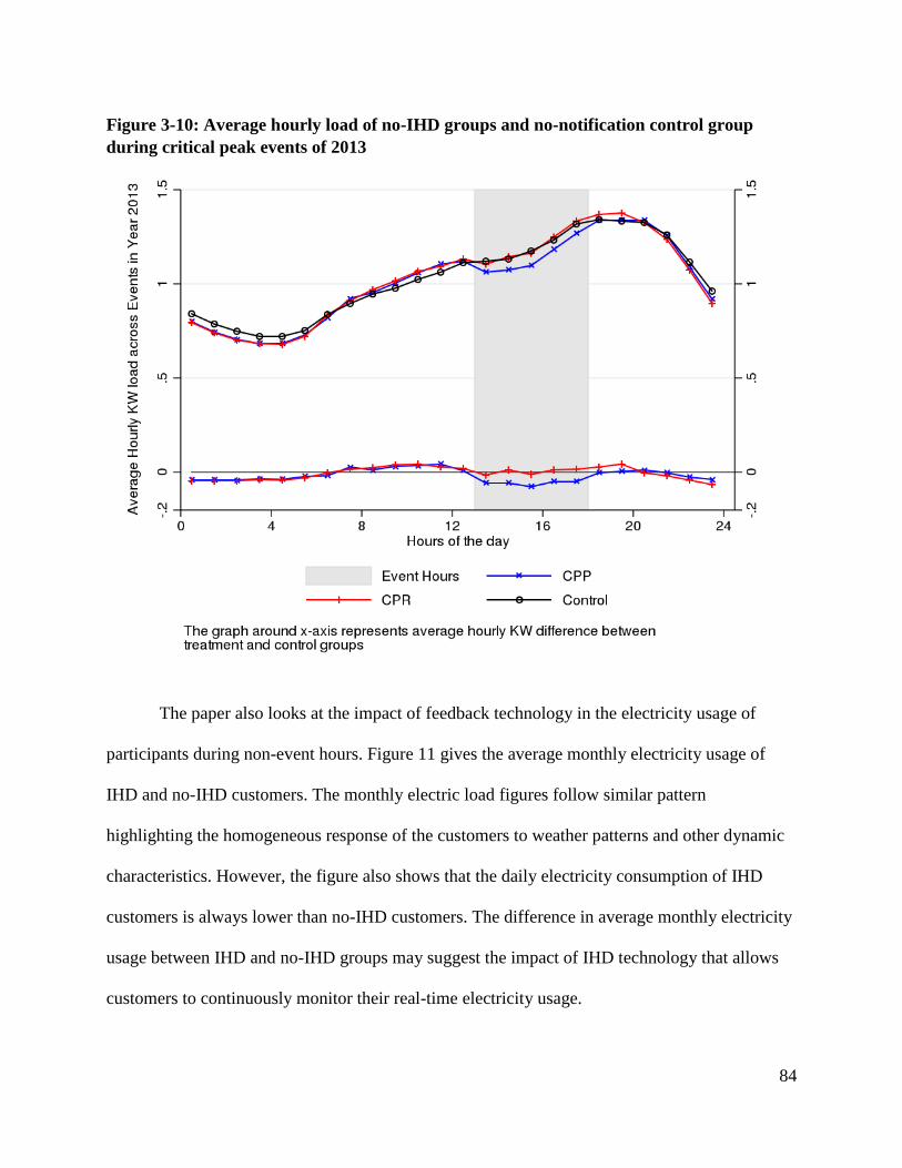
84
Figure 3-10: Average hourly load of no-IHD groups and no-notification control group
during critical peak events of 2013
The paper also looks at the impact of feedback technology in the electricity usage of
participants during non-event hours. Figure 11 gives the average monthly electricity usage of
IHD and no-IHD customers. The monthly electric load figures follow similar pattern
highlighting the homogeneous response of the customers to weather patterns and other dynamic
characteristics. However, the figure also shows that the daily electricity consumption of IHD
customers is always lower than no-IHD customers. The difference in average monthly electricity
usage between IHD and no-IHD groups may suggest the impact of IHD technology that allows
customers to continuously monitor their real-time electricity usage.

85
Figure 3-11: Average monthly KW load for customers with and without in-home-display
(IHD) systems
Moreover, figure 12 presents average monthly load (kW) by treatment groups. The
monthly load patterns of various treatments are very similar. The monthly load consumption of
CPP and CPP-IHD customers are lower during the month of August 2012 as compared with CPR
and control group customers. It might be because of the change in their consumption behavior
after installing IHD equipment. However, this behavior fades away after few weeks.

86
Figure 3-12: Average monthly KW load for customers by treatment group
Result and Analysis 7.
This section presents the regression results analyzing the consumers’ behavior due to the
critical peak events. We start with estimating the potential peak load reduction at different time
periods surrounding the critical event period with the help of RCT approach. Then, we conduct
RED analysis in order to incorporate CPP customers that declined to participate in the pilot
study. Tables 7 and 8 present regression results from RCT and RED analyses, respectively.
Similarly, the paper includes the regression results, tables 9 – 11, from persistence analysis
conducted at three different time horizons – within critical peak events, event-to-event, and year-
to-year. We also estimate the impact of continuous feedback technology in the monthly

87
electricity consumption. All the models include customer-level fixed effects. Standard errors are
robust and clustered at the customer-level to control for the serial correlation.
7.1 Peak Load Analysis
7.1.1 RCT and RED Analysis
The regression results from table 7 show that customers hourly load reduction during the
critical peak period is statistically significant. Pilot study participants of Rutland, VT decreased
0.034 kW per hour on average as compared with control with no-notification customers during
the five-hour critical peak event period. Similarly, during the six-hour prior to the events called
and 24-hour after the event, the hourly consumption of electricity were higher as compared with
the control with no-notification group customers. On average, treatment group participants
increased electricity usage by 0.069 kW and 0.147 kW than the control group participants during
the pre- and post-event periods respectively.
The study’s primary interest is to predict the impact of different treatment and
information rates in real-time electricity usage. The coefficient estimates of interaction variables
between critical event hours and treatment groups, 𝛽3 in equation 1, show that customers in
different rates responded distinctly. On average, residents on CPR treatments decreased hourly
load by 0.045 kW and CPR customers equipped with IHD reduced 0.068 kW of hourly load. The
log-linear econometric model suggests that CPR group customers’ peak load reduction is 5.5 –
6.8 percent higher than the control group customers. The response of CPP treatments customers
is larger than the CPR customers. Customers in the CPP rate reduced hourly electric usage by
0.051 kW during the event period. The maximum hourly load reduction is seen among CPP
customers with IHD technology. On average, CPP with IHD customers decreased 0.103 kW of
electric load per hour, 8.5 percent more than control group customers, during the critical peak

88
events of the first year of the study. Please note that, responses of CPR-IHD and CPP-IHD group
customers are only statistically significant among the responses of different treatment groups.
The paper also examines the impact of treatment rates during the periods surrounding the
critical events. The results show that there is no statistical significant difference in hourly load
usage between treatment and control group customers during both periods - six-hour window
preceding the start of the event and 6 hours after the end of the event.
The RED analysis results are presented in table 8. The analysis, taking CPP customers
that declined to participate or dropped out during the study into account, shows that the hourly
load reduction by CPP customer is larger than the one predicted by RCT analysis. On average,
CPP customers decreased 0.116 kW of electric load per hour, which is 1.12 times larger than
predicted by the RCT approach. During the first year of the study, 155 participants in critical
peak treatment rate, in which 113 customers are in CPP group (25.4 % of the total CPP treatment
group) and 37 residents belong to CPP with IHD customers (22.1 % of the CPP-IHD group),
declined to participate after the treatment groups were revealed to them. Similarly, during the
period of the second year, 37 CPP customers (11.5 %) and 21 CPP-IHD customers (12.2 %)
dropped out of the pilot study.
The second way to account customers that declined to participate or dropped out of the
program is with the help of local average effect (LATE) method. In this method, we divide the
estimates of RCT analysis by the difference in the fraction of customers who took up the rate
between the encouraged group and the non-encouraged group. The accepted percentage for CPP
and CPP-IHD groups are 80.75% and 82.89%, respectively. The coefficients of CPP and CPP-
IHD customers during critical peak event hours are comparable across three different methods.

89
LATE method suggests that CPP treatment group customers reduced 0.0630 kW as compared
with the control group customers during event hours. Similarly, CPP with IHD customers’
reduction is 0.125 kW during the same period.
Table 3-7: Regression Results for Randomized Control Treatment Analysis
DB DE DA
0.069*** -0.034 0.147***
(0.016) (0.023) (0.019)
CPR 0.025 -0.006 -0.045 -0.032
(0.022) (0.021) (0.031) (0.026)
CPR with IHD -0.013 0.006 -0.068* -0.028
(0.025) (0.027) (0.036) (0.030)
CPP -0.013 0.033 -0.051 0.002
(0.023) (0.022) (0.031) (0.026)
CPP with IHD -0.017 0.024 -0.103*** 0.010
(0.026) (0.027) (0.036) (0.031)
Control with notification 0.011 -0.025 -0.053* -0.032
(0.008) (0.023) (0.032) (0.027)
Number of observations
note: *** p<0.01, ** p<0.05, * p<0.1
26,378,106
Regression results of RCT analysis - Years 2012 and 2013
Treatment Groups Only GroupInteraction of Group*Events

90
Table 3-8: Comparing coefficient estimates of CPP and CPP-IHD customers with RCT,
RED, and LATE methods
7.2 Persistence Analysis
The goal of persistence analysis is to estimate consumers’ electric usage pattern during
different time-horizons within the period of the study. Table 9 presents the persistence analysis
within different hours of the critical event periods. Similarly, event-to-event consumption
analysis is presented in table 10. And table 11 contains the regression results of year-to-year
persistence analysis.
The paper looks at the participants’ hourly response during the critical peak events
through hour-to-hour persistence analysis. The regression results are presented in table 9. The
interest of this analysis is to compare the customers’ hourly electricity usage during the critical
peak events. With the help of regression analysis, we predict the coefficient associated with the
interaction of critical peak event indicator with the hour dummy variables. The coefficient, 𝛼2 in
equation (4), gives the mean hourly differences of electricity consumption with the average
Independent Variables RCT
Analysis
RED
Analysis
LATE
Analysis
Before Event Hours * CPP 0.033 0.038 0.0406
(0.022) -(0.026) (0.028)
Before Event Hours * CPP - IHD 0.024 0.027 0.0285
(0.027) -(0.030) (0.032)
During Event Hours * CPP -0.051 -0.058 -0.0632
(0.031) -(0.036) (0.039)
During Event Hours * CPP - IHD -0.103*** -0.116*** -0.1247
(0.036) -(0.040) (0.043)
After Event Hours * CPP 0.002 0.002 0.0021
(0.026) -(0.030) (0.032)
After Event Hours * CPP - IHD 0.010 0.011 0.0118
(0.031) -(0.035) (0.038)

91
consumption from 12 – 1 pm of critical event days. Moreover, in order to control for the
temperature variations, we interact hour and event indicators with the hourly heat index.
The responses in residential power consumption during all event hours are statistically
significant. The result suggests that treatment-group customers hourly consumption increased by
0.030 – 0.036 kW with a degree increase in heat index during event hours as compared with the
control group customers. The more important result is the responses of different treatment groups
during event hours.
We look at each treatment groups’ electricity usages during the critical peak event hours.
The treatment indictor variables are interacted with hourly heat index to control for the possible
variations in electricity consumption due to the temperature change. The results of different
treatment rates show that the responses are consistent across different hours during the event.
This result is very encouraging for utility company because customers’ electricity usage behavior
does not die out during the event. We find that, even when we account for weather conditions,
customers in all four-treatment groups reduced electricity consumption during the event hours.
Any variations in persistence of response are small, amounting to 0.001 kW or less. This may
suggest that consumers are not micro-managing electricity consumption during peak events, but
rather are taking actions at a single point in time (such as adjusting thermostat settings) that
would ultimately lower their consumption levels during critical peak events.

92
Table 3-9: Persistence Analysis: Within Event Hours
Table 10 and figure 13 present the regression results of event-to-event persistence
analysis. Table 10 uses data for 2012 events, while figure 13 shows the change in hourly usage
due to planned critical events of 2013. The regression model uses heat index to control for
possible change in electricity consumption due to the weather variations. The results show that
customers’ reaction to the first and third critical peak events of 2012 were greater than the other
two events. On average, treatment group customers on critical peak event of September 14, 2012
reduced hourly load consumption by 2.288 kW as compared with the control with no-notification
customer group. Similarly, the decrease in hourly electricity consumption during September 25,
2012 is 2.362 kW. However, treatment group customers during critical peak events of 21
September, 2012 and 5 October, 2012 showed lower reduction, 0.777 kW and 0.916 kW
respectively.
Independent Variables Hour 13 Hour 14 Hour 15 Hour 16 Hour 17
Hour * Event-hour
Indicator * heat index0.030*** 0.034*** 0.038*** 0.036*** 0.034***
(0.001) (0.001) (0.001) (0.001) (0.001)
CPR -0.001*** -0.001** -0.001*** -0.001** -0.001**
(0.000) (0.000) (0.000) (0.000) (0.000)
CPR with IHD -0.001** -0.002*** -0.002*** -0.001*** -0.001**
(0.001) (0.001) (0.001) (0.001) (0.001)
CPP -0.002*** -0.002*** -0.002*** -0.002*** -0.002***
(0.000) (0.000) (0.000) (0.000) (0.000)
CPP with IHD -0.003*** -0.003*** -0.003*** -0.003*** -0.003***
(0.001) (0.001) (0.001) (0.001) (0.001)
No of Observations
note: *** p<0.01, ** p<0.05, * p<0.1
Group * Hour * Event-hour indicators * heat index interaction terms
26,427,323

93
Similarly, coefficients of interaction variable of event-hour indicators with the hourly
heat index show that the participants used more electricity during first and third critical peak
events. Among different treatment groups, the regression results shows that CPP with IHD
residents have statistically significant and consistent hourly load reduction across all four critical
peak events of 2012.
Table 3-10: Event-to-Event persistent analysis of year 2012
Figure 12 presents the mean difference of average electricity consumption between the
treatment and control group customers during different 2013 critical event days. The estimates
also contain the 95 percent confidence intervals. Please note that events 2 to 6 were called on
consecutive days from July 15 to July 19 of 2013. The responses do not show any particular
trend. We see that maximum reductions in second year occurred during the last three event
periods. The average temperatures during these three events are very closely related and lie in the
14-Sep 21-Sep 25-Sep 5-Oct
Event hours indicator -2.288*** -0.777*** -2.362*** -0.916***
(0.273) (0.104) (0.183) (0.138)
Event hours indicator *
heat index0.030*** 0.009*** 0.036*** 0.012***
(0.004) (0.002) (0.003) (0.002)
Group*Hour*Event Indicators*Heat Indecx interaction terms
PTR -0.001** -0.001 -0.001 -0.001*
(0.000) (0.000) (0.000) (0.000)
PTR with IHD -0.001*** -0.001 0.000 -0.001
(0.000) (0.000) (0.001) (0.000)
CPP -0.001 -0.001 -0.001 -0.001*
(0.000) (0.000) (0.001) (0.000)
CPP with IHD -0.002*** -0.001** -0.001** -0.001*
(0.001) (0.001) (0.001) (0.001)
Number of observations
note: *** p<0.01, ** p<0.05, * p<0.1
14,904,158

94
range of 80 F. Event 5 shows that treatment group customers used more electricity than control
group customers. It might be due to the shift in electricity usage from earlier event day (event 4)
to event 544
. Customers were unaware of critical peak event 5 during event 4 and may have
shifted some of the electricity intensive work to the next day. And treatment customers may have
completed the tasks on next day even though it was another critical peak event day.
Figure 3-13: Persistence Analysis – change in hourly electricity consumption (kW) – during
critical peak events of 2013
We then compare residential customers’ electricity consumption behavior between first
and second years of critical peak events. The relevant results are the interaction of treatment
group customers with year indicator at hours during the critical peak events. The regression
results show that all treatment groups’ consumption was lower in the second year’s event hours
than the first year’s one. However, the response of CPP and CPP-IHD customers is statistically
44
Events 4 and 5 occurred on July 17 and 18 of 2013.

95
significant. The electricity usage during event hours of second year of CPP customers is 0.219
kW lower than their usage in first years’ event hours. Similarly, in the second year event hours,
CPP-IHD customers consumed 0.278 KW lower than their consumption in the first year.
Although we compare power usage during first and second year of the study, we note that a
number of factors complicate the comparison, including the timing of the peak events in 2012
versus 2013 (the 2012 events were called in the fall, while the 2013 events were called during the
summer); very warm weather conditions during the summer of 2013; and a shift in the rate
treatment faced by some customers between 2012 and 2013.

96
Table 3-11: Persistence Analysis: year-to-year
Although the main objective of this study is to look at the peak load reductions due to
various treatment rates, we also analyze if the event days had any impact on daily electricity
consumption. In order to perform the analysis, we aggregated the hourly load data at the daily
level. The difference-difference regression results with customer-level fixed effects show that
treatment groups’ daily electricity consumption during event days is lower than the control
groups ones. The regression results are present in table 12. The daily electricity usage of CPR
Independent Variables Results
Heat Index (F) -0.003***
(0.000)
Year indicator - 1 if year 2013; 0 if year 2012 0.138***
(0.012)
Year indicator * Before event Hours 0.141***
(0.009)
Year indicator * Event hours 0.416***
(0.032)
Year indicator * After event hours 0.351***
(0.009)
Year indicator * During event hours * CPR Customers -0.001
(0.046)
Year indicator * During event hours * CPR-IHD
Customers-0.059
(0.052)
Year indicator * During event hours * CPP Customers -0.219***
(0.043)
Year indicator * During event hours * CPP-IHD
Customers-0.278***
(0.048)
Year indicator * During event hours * control-
notification Customers-0.063
(0.043)
Number of observations 26,427,323
note: *** p<0.01, ** p<0.05, * p<0.1

97
treatments – both without IHD and with IHD – is at least 1 kWh lower than the control group
customers. For CPP group, even though the coefficients are negative, we fail to show statistical
significance in daily electricity usage with the control group.
Table 3-12: Daily load analysis during event and non-event days
7.3 Hourly Load Analysis of Transitioning Group
The study also conducted a separate analysis for transitioning treatment group of customers
on hours surrounding critical peak events. A group of participants were transferred from CPR
(first year) to CPP (second year) treatment rates. This is an example of ‘carrot-stick’ approach –
customers are in voluntary rebate program during the first, but are placed into ‘mandatory’
Independent Variables Year 1 Year 2 Both years
Average Daily Heat Index (HI) -0.121*** -0.109*** -0.113***
(0.004) (0.004) (0.004)
Average Cooling degree hours -0.862*** -3.546*** -1.581***
(0.070) (1.168) (0.121)
Total Daily Cooling degree hours 0.003*** 0.008*** 0.004***
(0.000) (0.002) (0.000)
Event Days -1.725*** 1.940*** 0.746**
(0.244) (0.448) (0.341)
Event Days * CPR -0.279 -0.409 -0.944**
(0.302) (0.683) (0.458)
Event Days * CPR-IHD -0.065 -0.788 -1.006*
(0.325) (0.792) (0.531)
Event Days * CPP 0.042 -0.836 -0.653
(0.325) (0.614) (0.463)
Event Days * CPP-IHD -0.513 -1.208* -0.792
(0.404) (0.706) (0.533)
Event Days * notification -0.092 -1.323** -1.212***
(0.332) (0.647) (0.463)
Number of observations 649,311 527,550 1,176,861
Adjusted R2 0.054 0.071 0.058
note: *** p<0.01, ** p<0.05, * p<0.1

98
pricing structure in the second year. We noticed a large number of customers dropping out of the
pilot study during the second year.
Table 3-13 presents regression results of transitioning group customers analyzing their hourly
electricity consumption. Transitioning customers responded more actively to CPP than CPR
treatment by reducing usage during event hours and by shifting their electricity load to hours
surrounding critical peak events. The same IHD customers when placed in CPP rate reduced
hourly electricity consumption by 0.11 kWh than when they faced CPR treatment. The results
also show that transitioned treatment groups used more electricity before- and after critical peak
event hours of second year as compared with the first year. The result of increase in usage before
and after event hours and reduction in consumption during event hours indicate a higher impact
of price treatment than rebate treatment.

99
Table 3-13: Hourly load analysis of transitioning treatment groups
7.4 Energy Consumption Analysis
We also assess the impact of IHD technology on customers’ electricity consumption. The
regression results are presented in table 9 separately for 2012 and 2013. The regressions use
month-fixed effects in order to control for the heterogeneity in electricity consumption that may
arise due to weather affects. The first column presents the regression results for 2012, whereas
the second column consists of 2013 results. As a robustness check, we also looked at the effect
Independent Variables
Regression
coefficients
Heat Index -0.003***
(0.000)
Cooling degrees 0.032***
(0.001)
Cumulative Cooling degrees -0.000**
(0.000)
Year 2 Indicator: Year 2 = 1; Year 1 = 0 -0.017**
(0.007)
Year 2 Indicator * CPR-CPP -0.012
(0.011)
Year 2 Indicator * CPR-CPP-IHD 0.001
(0.014)
Before Event Hours* Year 2 Indicator * CPR-CPP 0.197***
(0.026)
Before Event Hours* Year 2 Indicator * CPR-CPP-IHD 0.114***
(0.032)
During Event Hours* Year 2 Indicator * CPR-CPP -0.008
(0.034)
During Event Hours* Year 2 Indicator * CPR-CPP-IHD -0.110***
(0.042)
After Event Hours* Year 2 Indicator * CPR-CPP 0.177***
(0.028)
After Event Hours* Year 2 Indicator * CPR-CPP-IHD 0.149***
(0.037)
Number of observations 9,747,996
Fixed Effects Yes
note: *** p<0.01, ** p<0.05, * p<0.1

100
of IHD on daily electricity consumption and the regression results are very similar. The results of
daily electricity usage are presented in the appendix.
The results show that the impact of feedback technology in monthly electricity
consumption is considerable and statistically significant. On average, during the first year,
customers with IHD technology decreased monthly electricity usage by 34.6 kWh as compared
with the average monthly usage of customers without the continuous feedback system. However,
the impact of IHD equipment in 2013 is considerably lower than seen in 2012 – the monthly
electricity usage customers with the feedback technology is 12.7 kWh lower than the customers
that do not possess the equipment. The higher impact seen in for 2012 may have to do with
timing of installation of IHD technology. GMP distributed the IHD system during August 2012
right after the hot summer days. The model puts IHD customers in non-IHD group from March
2012 to July 2012 limiting the analysis for estimate the impact of technology during relatively
milder weather.
We think the results of 2013 gives better estimates of the impact of IHD in monthly
electricity usage. It is mainly for two reasons – the data is available for year around, and
customers have IHD for at least few months and their behavior may be consistent. The log-linear
model shows that this decrease in monthly load usage amounts to 2.0 – 5.3 percent reduction as
compared with the non-IHD customers. The relevant study by Houde et al. shows the continuous
feedback technology reduces electricity usage by 5.7%.

101
Table 3-14: Impact of IHD technology in monthly electricity usage (kW)
Conclusion 8.
We study Green Mountain Power’s customers’ electricity consumption patterns in a
response to the critical peak events during two-year long pilot study. Critical peak events are
called when utility company anticipates very high demand during summer. Participants are
notified by 6 pm of prior day before each critical event day. In total, GMP called four events
during the first year and another ten events in the second year. According to the participants’
treatment rates, customers either receive payment for lowering electricity usage below their
baseline or have an opportunity to reduce their electricity bill by decreasing usage in order to
avoid high pre-determined critical peak pricing. Moreover, we also analyze the change in total
electricity consumption due to the installation of continuous feedback technology.
The analysis of customer-level electricity consumption shows that incentive based
demand response programs has statistically significant impact in reducing peak load. Regardless
of weather, both the CPR and CPP rate groups measurably reduced electricity usage, in the range
of 6.0 – 10.3 percent, during the declared critical peak event. The CPR rate reduces peak load
Independent Variables Year 1
(2012)
Year 2
(2013)
Average Cooling degree hours -37.402** 45.924**
(17.591) (19.250)
Average heat index 9.558*** 5.086
(2.714) (3.558)
Customers with IHD -34.616*** -12.707**
(9.240) (6.264)
Number of observations 22,313 19,490
Adjusted R2 0.072 0.218
Month-fixed effects Yes Yes
note: *** p<0.01, ** p<0.05, * p<0.1

102
usage by 6.0 – 7.7 percent whereas the impact of CPP treatment rate is larger. The decrease in
electricity consumption by CPP rate participants is between 6.8 and 10.3 percent during the
critical peak events. The results also suggest that participants with IHDs show larger responses
during non-event hours than customers facing similar electricity rates but are not equipped with
the IHDs.
The results indicate that customers on CPR reduced their average hourly loads by 0.038
to 0.081 kW (6.0 – 7.7 percent), relative to a control group that was not notified of peak events
and was not placed on any special rate during the critical peak event hours. Besides RCT
analysis, we also conduct RED and LATE analysis for CPP related customers in order to account
for the participants that opted-out of the pilot study. Customers on CPP exhibited larger average
hourly load reductions of 0.045 to 0.142 kW (6.8 to 10.3 percent), relative to the control group.
Customers equipped with In-Home Displays (IHDs) generally exhibited larger reductions
during peak events. While CPR customers equipped with IHDs exhibited reductions around 20%
larger than CPR customers without the IHD, CPP customers equipped with the IHD exhibited
critical peak reductions nearly twice as large, on average, as CPP customers without the IHD.
Moreover, we also study the impact of IHD technology in monthly electricity usage. On average,
IHD equipped participants’ monthly energy consumption is 2.0 to 5.3 percent lower than the
monthly energy usage of non-IHD customers.
Participants’ electricity usage patterns differ across different critical peak event periods.
We observed that customer responses were quite persistent during the hours of the critical peak
event, indicating that customers take response actions at the beginning of critical peak times or
prior to the start of the critical peak period, rather than managing their electricity usage on an
hour-to-hour basis during critical peak events. Persistence of customer responses across critical

103
peak events was less consistent.
None of the rate and IHD treatments induced a persistent response across multiple critical
events. Therefore, the use of rate structures and information feedback alone provide insufficient
motivation for consumers to reduce demand in any consistent way across multiple event periods.
Based on our evaluation of GMP’s DR programs during 2012 and 2013, neither critical peak
pricing nor rebates are themselves sufficient to substitute for new capacity to meet resource
adequacy requirements.
We acknowledge that our study lacks a way to measure the long-term energy efficiency
adjustments that customers may make due to the impact of critical peak events and IHD
technology. Even though we are able to analyze consumers’ behavior due to various treatment
rates, our study undermines the impact of long-run emergency DR programs. The impact of DR
programs increases with the length of the program. Since the short-term electricity demand is
more inelastic than long-term demand, customers’ peak load reduction in the short-term may not
be as significant as in the long run. King and Chatterjee (2003) find that the median price
elasticity of electricity demand in short-run and long-run to be -0.2 and -0.90 respectively. A
long term DR program may encourage customers to reduce electricity usage by purchasing
energy efficient appliances and we might be able to see large peak load reductions.

104
References 9.
Albadi, M. H., & El-Saadany, E. F. (2008). A summary of demand response in electricity
markets. Electric Power Systems Research, 78(11), 1989-1996.
Branch, E. R. (1993). Short run income elasticity of demand for residential electricity using
consumer expenditure survey data. The Energy Journal, 111-121.
Cappers, P., Goldman, C., & Kathan, D. (2010). Demand response in US electricity markets:
Empirical evidence. Energy, 35(4), 1526-1535.
Demand Response: California Public Utilities Commission. (2013). Retrieved September 5,
2013, from http://www.cpuc.ca.gov/PUC/energy/Demand Response/
Voluntary Load Response. (2013). Retrieved September 5, 2013, from
http://www.ercot.com/services/programs/load/vlrp/
State of Vermont Partners with EnerNOC for Demand Response. (2008, October 2). Retrieved
September 5, 2013, from
http://investor.enernoc.com/releasedetail.cfm?ReleaseID=338112
Faruqui, A., Hajos, A., Hledik, R. M., & Newell, S. A. (2010). Fostering economic demand
response in the Midwest ISO. Energy, 35(4), 1544-1552.
Federal Energy Regulatory Commission. (2012). Assessment of Demand Response and Advanced
Metering. Retrieved from FERC website: http://www.ferc.gov/legal/staff-reports/12-20-
12-demand-response.pdf
Herter, K., McAuliffe, P., & Rosenfeld, A. (2007). An exploratory analysis of California
residential customer response to critical peak pricing of electricity. Energy, 32(1), 25-34.

105
Herter, K. (2007). Residential implementation of critical-peak pricing of electricity. Energy
Policy, 35(4), 2121-2130.
Herter, K., & Wayland, S. (2010). Residential response to critical-peak pricing of electricity:
California evidence. Energy, 35(4), 1561-1567.
Houde, S., Todd, A., Sudarshan, A., Flora, J. A., & Armel, K. C. (2013). Real-time Feedback
and Electricity Consumption. Economics, 95(9), 1082-1095.
Independent System Operator of New England. (2013b). Key Grid and Market Stats.
Retrieved September 2013, from http://www.iso-ne.com/about/what-we-do/key-stats
Independent System Operator of New England. (2013a). Section III, Appendix E1, Market
Rule1. Retrieved September 2013, from http://www.iso-
ne.com/regulatory/tariff/sect_3/mr1_append-e.pdf
King, C. S., & Chatterjee, S. (2003). Predicting California Demand Response. Retrieved from
Public Utilities Fortnightly website:
http://www.americanenergyinstitutes.org/research/CaDemandResponse.pdf
Spees, K., & Lave, L. B. (2007). Demand response and electricity market efficiency. The
Electricity Journal, 20(3), 69-85.
NYISO Auxiliary Market Operations. (2013). Emergency Demand Response Program Manual.
Retrieved September 2013, from:
http://www.nyiso.com/public/webdocs/markets_operations/documents/Manuals_and_Gui
des/Manuals/Operations/edrp_mnl.pdf

106
Office of Energy Efficiency and Renewable Energy. (2013). Federal Energy Management
Program. Retrieved September 2013, from:
http://energy.gov/node/782456/financing/eip_vt.html
PJM. (2013a). Demand Response. Retrieved September 2013, from:
http://www.pjm.com/markets-and-operations/demand-response.aspx
PJM. (2013b). Retail Electricity Consumer Opportunities for Demand Response in PJM’s
Wholesale Markets. Retrieved September 2013, from:
http://www.pjm.com/~/media/markets-ops/dsr/end-use-customer-fact-sheet.ashx.
Stern, P. C. (1992). What psychology knows about energy conservation. American
Psychologist, 47(10), 1224.

107
Appendix 10.
Table 3-15: Impact of IHD technology in daily electricity usage
Table 3-16: Analysis for hours with Heat Index greater than 80 F -Year 2
Independent VariablesLoad
(kWh)
Load
(kWh)
Log Load
(log(kWh))
Log Load
(log(kWh))
Total daily cooling degree hours 0.175*** 0.218*** 0.018*** 0.018***
(0.048) (0.040) (0.003) (0.003)
Average daily heat index -0.732*** -0.789*** -0.068*** -0.070***
(0.040) (0.025) (0.002) (0.002)
Customers with IHD -1.079*** -0.504** -0.034*** -0.027**
(0.056) (0.218) (0.003) (0.011)
Constant 35.922*** 16.365*** 3.300*** 2.514***
(13.583) (0.627) (0.748) (0.039)
Number of observations 649,311 649,311 645,971 645,971
Adjusted R 2 0.035 0.090 0.026 0.089
Customer-fixed effects No Yes No Yes
Day-of-the-year fixed effects No Yes No Yes
note: *** p<0.01, ** p<0.05, * p<0.1
Independent Variables Results
Heat Index (F) 0.004*
(0.002)
Cooling degree days 0.018***
(0.002)
Before Event hours 0.214***
(0.008)
During Event hours 0.130***
(0.009)
After Event hours 0.288***
(0.009)
No of Observations 631,580
note: *** p<0.01, ** p<0.05, * p<0.1

108
Figure 3-14: Daily load profile during Event days of 2012 for IHD groups

109
Figure 3-15: Daily load profile during Event days of 2012 for non-IHD groups

110
Figure 3-16: Daily load profile during Event days of 2013 for IHD groups

111
Figure 3-17: Daily load profile during Event days of 2013 for non-IHD groups

112
Chapter 4: Analysis of Load and Price patterns in the U.S.
Electricity Sector
Abstract
This paper analyzes hourly electricity loads and marginal costs of electric entities with of
extreme value theory (EVT), a concept widely used in the financial sector. For each year’s
hourly data of balancing authorities and utilities, we fit generalized extreme value (GEV)
distribution and estimate the parameters of the distribution with an aim of comparing how these
parameters have changed over time and market regions. We also account for the time
dependencies, seasonalities, and near-time clustering present in the electricity markets – both for
electricity load and prices – with the help of autoregressive conditional hetereskedastic models.
that the results show that the distributions of hourly load and lambda values are fat tailed. Hourly
lambda values have more extreme values generating fatter tails than hourly electricity load. We
also show that extreme tail quantiles estimated with the GEV parameters at different percentile
levels are comparable with the percentiles of actual observations.
Keywords: Extreme Value Theory, Generalized Pareto Distributions, AR/GARCH, electricity
markets

113
Introduction 1.
The United States electricity sector has undergone massive changes over the last few
years. The deregulation of the industry has changed the way electricity is being traded and
returns received by utilities. The emphasis on clean energy policy and climate change has
increased grid-connected renewable generation, which in turn raises intermittency issues.
Limited storability of electricity makes meeting dynamic electricity demand, especially during
peak demand period, challenging and economically inefficient.
For a reliable and stable electricity system, utilities should be capable of meeting both
total electricity demand and peak demand at all times. Since the safety and reliability of
electricity systems are both compromised if there is a sudden change in electricity markets, there
is a need to analyze how electricity transaction and load patterns, especially during high demand
periods, have changed within and across different electricity markets. The study analyzes the
periods of peak electricity demands and very high electricity prices using extreme value theory
(EVT). For each year’s hourly data of balancing authorities and utilities, we fit generalized
extreme value (GEV) distribution and estimate the parameters of the distribution with an aim of
comparing how these parameters have changed over time and market regions.
The electricity usage pattern is changing; the average peak demand growth is outpacing
total electricity demand growth (citation needed). Spees (2008) points out that the fraction of
capacity serving just peak load has increased during 1980 – 2006 period. Using hourly load data
of New England Independent System Operator (NE-ISO) regions, Spees shows that 15% of the
total capacity of ISO-NE ran only 0.9% of the time or less for the year of 200645
. The recent
45
This calculation doesn’t even account 8% reserve margin.

114
trend of increasing gap between the peak demand and average electricity demand raises few
concerns. Only peak load serving capacity increase results in economic inefficiency since these
infrastructures run only a few hours per year. New investments in both electricity generation and
transmission sectors are capital-intensive. Analysis of peak electricity consumption pattern is
important for planning and investment purpose since the load growth is the main reason for
utilities to acquire additional generation sources (Berry, 2008).
Extreme value theory is a well-studied subject, however its use in the electricity sector is
limited. Fuller (1914) and Griffith (1920) conducted the earliest work on the methods of
application of EVT. Fisher and Tippet (1928) made a major development by concluding that
extreme limit distribution can be only of three types. Gnedenko (1943) presented rigorous
foundation for EVT and Gumbel (1958) proposed applications of EVT, which was previously
treated theoretically. Few of the recent books such as Kotz and Nadarajah (2000) and Coles
(2001) provide excellent theory and review of extreme value distributions.
In the electricity sector, most of the literatures on extreme value theory focus on
modeling and estimating wholesale electricity prices of a single market region. Bosco et al
(2007), Huisman and Kilic (2011), Bystrom (2005) and Chan and Gray (2006) use generalized
extreme value distribution to AR-GARCH filtered price change series to investigate the tails of
the electricity price change distribution. Spees (2008) treats peak load as extreme value to predict
the total capacity necessary to serve forecasted load in the NE-ISO region. Spees (2008) then
calculates the total capacity required to ensure meeting peak demand of NE-ISO with the help of
EVT theory projected distribution around peak load. Our paper serves a different purpose. The
paper provides a comprehensive analysis of extreme tail characteristics of different market
regions’ hourly electricity load and prices.

115
We use EVT to analyze hourly electricity load of the US electricity providers. First, the
paper fits the GEV distribution to predict the parameters and analyze how these parameters
change over time and geographic locations. This allows comparing the usage of generation
capacity within one electric jurisdiction over the years and also between different electric entities
and balancing authorities. Besides estimating the parameters of the most appropriate distribution,
we can also predict the return value, that is the maximum value that the electricity price or load
can reach in future. This helps us determine or forecast massive changes in future electricity
demand. We also address time dependencies of hourly electricity load with the help of
autoregressive conditional heteroskedastic models.
We also estimate extreme value parameters of hourly system lambda values of various
balancing authorities. System lambda represents the marginal cost of the generating plant that
meets the last MWh of electricity demanded. Wholesale electricity price comprises of system
lambda and transmission congestion cost. We use hourly system lambda as a proxy for electricity
prices. Similarly, balancing authority is the responsible entity within a metered area for reliable
planning and operation of bulk power system. Its prime function is to continually balance the
control area’s scheduled and actual electricity interchange by dispatching generation units used
for regulation.
The results demonstrate that the distributions of hourly load and lambda values are fat
tailed. Hourly lambda values have more extreme values generating fatter tails than hourly
electricity load. This is understandable because hourly load has upper limit due to physical
constraints such as transmission lines and generation capacity. We also estimate extreme tail
quantiles with the help of generalized extreme value parameters. The results show that extreme

116
tail quantiles estimated with the GEV parameters at different percentile levels are comparable
with the percentiles of actual observations
However, there are few caveats in our study in terms of data availability and use of
common method across geographic regions. The data availability dictates the inclusion of
electricity providers and balancing authorities in our analysis. The main source of data is the
Federal Energy Regulatory Commission (FERC) 714 form. The hourly load and electricity data
are not available continuously for all years. In order to analyze extreme occurrences of hourly
electricity load, we are able to include 52 electricity providers for 2000 – 2012 and 118
electricity providers for 2006 – 2012 period. Similarly, for analyzing extreme changes in hourly
lambda values, we have 16 balancing authorities for 2000 – 2012 period and 48 for 2006 – 2012
period. Moreover, we use a single method to estimate extreme value and autoregressive
conditional heteroskedastic parameters for all electricity entities available in our study even
though electric entities differ in many ways – size, type, market regulation, state policies.
The rest of the paper follows with the overview of the US electricity sector in section 2.
We include brief background of extreme value theory and its implications in the electricity sector
in section 3. Similarly, section 4 describes hourly electricity data and conducts tail analyses. In
section 5, we compare generalized extreme value parameters across different market regions and
years. We conclude in section 6.
Overview of United States Electricity Sector 2.
Electricity is significant part of the energy consumption that drives economy and
environment. The total electricity generation of United States in 2012 is 4.047 TWh with average
residential electricity price of 9.84 cents/kWh- ranging from 6.44 cents/kWh in Idaho to 15.89

117
cents/kWh New York, 16.35 cents/kWh in Connecticut (EIA, 2012a). There are various forms of
electricity providers depending on the state, size, and regulations. In 2012, there were 3262
electricity providers comprising of 2006 publicly owned utilities, 193 investor-owned utilities
(IOUs), 973 cooperatives, and 181 power marketers. Even though the number of IOUs is
significantly smaller than publicly owned utilities, IOUs are responsible for 40 % of 4.167 TWh
of generation and publicly owned utilities generate 10.4 %. Other significant portion of
generation comes from the non-utility generators. (2013-14 Annual Directory and Statistical
Report, American Public Power Association)
The federal regulatory bodies, Federal Energy Regulatory Commission (FERC) and
North American Reliability Corporation (NERC), oversee reliability, sales, and transmission of
electricity in United States. The Federal Energy Regulatory Commission (FERC) is an
independent body that regulates the interstate transmission and wholesale sales of electricity. The
Energy Policy Act of 2005 gave more responsibilities to FERC in the areas of smart grid,
demand response, and integration of renewables. The North American Reliability Corporation
ensures the reliability of the bulk power system by developing and enforcing the Reliability
Standards. NERC regions include all of US territory and some parts of southern Canada. In
figure 1, we show NERC jurisdiction over US and Canada.

118
Figure 4-1: North American Electric Reliability regions (EIA, 2012b)
The United States mainly consists of two types of electricity markets – regulated and
deregulated. The regulated market has a vertically integrated model responsible for generation,
transmission, and distribution systems. The regulated market can also have a separate entity
responsible for the distribution section of the electricity market. The second electricity market
type is based on competitive model in both wholesale and retail electricity sectors and covers 66
% of the total U.S. consumers (Neenan and Flaim, 2010).
In regulated market, which was predominant before restructuring, a single agent has the
responsibility of electricity generation, transmission, and distribution for a certain rate of return
on investment. However, consumers are responsible for securing commodity and transmission in
the deregulated market. Similarly, in the competitive market, generators can sell their output
through spot market, bilateral contracts, or directly to retail customers.
The key difference in these two markets is the way electricity prices are set. The price in
the restructured market is ‘forward-looking’ reflecting the marginal costs and transmission
congestions and does not consider sunk costs. Whereas, regulated prices are based on average
3
competitive model in both wholesale and retail electricity markets that covers 66 % of the total
U.S. consumers (Electric Power Research Institute, 2009). In the regulated market, which was
predominant before restructuring started, a single agent has the responsibility of electricity
generation, transmission, and distribution for a certain amount of rate of return on investment.
Consumers are responsible for securing commodity and transmission in the deregulated market.
Similarly, in the deregulated market, generators can sell their output through spot market,
bilateral contracts, or directly to the retail customers. The key difference in the two types of the
market is the way electricity prices are set. The price in the restructured market is ‘forward-
looking’, reflect the marginal costs and transmission congestion (?), and don’t consider the sunk
costs, whereas regulated prices are based on the average, historic costs. However, there is some
similarity among two markets as “both operate in deregulated wholesale commodity and
transmission markets and both have non-competitive distribution” .
Electricity is a complex commodity –laws of physics govern the its flow and economics
dictates the dispatch. The electricity sector, especially operating in the competitive market, bears
price and demand risks that arises from the nature of the product itself. Generally the risks
associated with the electricity markets can be divided into four categories – volume, regulatory,
transaction, and market. Some of the risks generate from lack of grid-level storage, demand
variations, lack of accurate weather predictions, use of multiple fuel sources, production
constraints, regulation, and reliability measures. Moreover, the new energy policies such as
renewable portfolio standards, production tax credits, demand response and energy efficiency
programs, incentives promoting distributed generation also increases the burden to maintain
reliability standards. The increase in risks, driven by market, regulations, and politics, makes
providing reliable and continuous supply of electricity a challenging job.
Managing risks and also maintaining reliability and safety standards at the same time is
challenging task. This study provides a different approach to analyze historic electricity demand
and lambda data. The use of extreme value theory to study the extreme events of electricity
demand and prices help forecast the similar events in the future. This may help electricity
providers to prepare for such changes accordingly.
- The risks and uncertainties in the electricity sector increases with the rise in the
number changes. The sector has seen numerous changes in recent years.
NERC Region prior 2005 NERC Region after 2005
Suman Gautam 6/6/14 3:59 PM
Deleted:'a
Suman Gautam 6/6/14 3:59 PM
Deleted:' Whereas,
Suman Gautam 6/6/14 3:59 PM
Deleted:'in the deregulated market,
Suman Gautam 6/6/14 4:00 PM
Deleted:' c
Suman Gautam 6/6/14 3:59 PM
Deleted:'the
Suman Gautam 6/6/14 4:00 PM
Deleted:'G
Suman Gautam 6/6/14 4:01 PM
Moved (insertion) [2]
Suman Gautam 6/6/14 4:01 PM
Deleted:' ..."[2]
Suman Gautam 6/6/14 4:01 PM
Formatted: Normal, No bullets ornumbering
Suman Gautam 6/6/14 4:01 PM
Moved'up'[2]:'The key difference in the two
types of the market is the way electricity prices
are set. The price in the restructured market is
‘forward-looking’, reflect the marginal costs
and transmission congestion (?), and don’t
consider the sunk costs, whereas regulated
prices are based on the average, historic costs.
Suman Gautam 6/6/14 4:02 PM
Deleted:'P
Suman Gautam 6/6/14 4:03 PM
Deleted:'electricity market
Suman Gautam 6/6/14 4:15 PM
Moved (insertion) [3]
Suman Gautam 6/6/14 4:23 PM
Formatted: Normal, Indent: First line: 0.5", No bullets or numbering
Suman Gautam 6/6/14 4:15 PM
Moved'up'[3]:'Generally the risks associated
with the electricity markets can be divided into
four categories – volume, regulatory,
transaction, and market.
Suman Gautam 6/6/14 4:18 PM
Moved (insertion) [4]
Suman Gautam 6/6/14 4:18 PM
Deleted:'The increase in risks, driven by ..."[3]
Suman Gautam 6/6/14 4:19 PM
Deleted:'way
Suman Gautam 6/6/14 4:23 PM
Deleted:' to analyze extreme events – both in ..."[4]
Suman Gautam 6/6/14 4:23 PM
Deleted:'…

119
and historic costs. However, there are some similarities between two markets – both operate in
deregulated wholesale commodity and transmission markets and both have non-competitive
distribution.
Electricity is a complex commodity – physics governs its flow and economics dictates the
dispatch. The electricity sector, especially operating in the competitive market, bears price and
demand risks that arises from the nature of the product itself. Generally the risks associated with
the electricity markets can be divided into four categories – volume, regulatory, transaction, and
market. Some of the risks generate from demand variations, use of multiple fuel sources,
production constraints, regulation, reliability measures, and lack of grid-level storage and
accurate weather predictions. Moreover, new energy policies such as renewable portfolio
standards, production tax credits, demand response and energy efficiency programs, incentives
promoting distributed generation also increase burden to maintain reliability standards. The
increase in risks, driven by market, regulations, and politics, makes providing reliable and
continuous supply of electricity a challenging job.
Managing risks and also maintaining reliability and safety standards at the same time is a
challenging task. This study provides a different approach to predict future spikes by analyzing
historic electricity demand and lambda data. This study helps electricity providers to prepare for
extreme situations.
Extreme Value Theory and Implication in the Electricity Sector 3.
The hourly electricity demand varies periodically – daily, weekly, and seasonally. In
daily basis, electricity demand is high during daytime. The electricity usage is high during
summer season, mainly demand driven by the use of air conditioner and long daylight. The

120
periodic variations in the electricity load generate extreme values. Figure 2 gives hourly load of
PJM region during period of 2000 – 2012 in a time-series plot. We can see that the hourly load
values are extremes in few instances throughout the year.
Similarly, the nature of electricity leads to non-constant and high electricity marginal
costs. Some of the main properties are non-storability, inflexibility in changing generation
amount, and limitations in transferring bulk amount of electricity. Figure 3 contains the time-
series plot of hourly lambda values of New York ISO (NYISO) region. The figure shows that the
extreme positive lambda values are very high compared to the median lambda values. Moreover,
the high sample kurtosis values of hourly electricity load and lambda values suggest that the
distributions have fat tails.
Figure 4-2: Hourly load (GW) plot of PJM region from 2000 to 2012

121
Figure 4-3: Hourly lambda ($/MWh) of New York ISO from 2006 to 2012
There are at least three ways to estimate Value-At-Risk (VAR). They are variance-
covariance method, historic simulations, and EVT. The extreme value fits extreme quantiles
better than conventional approaches and thus is better method for observations with fat tails
(Embrechts, 2000).
Extreme value theory (EVT) allows us to model extreme and rare events of independent,
identically distributed random variables. It is widely used in finance, hydrology, and
meteorology sectors. Unlike classical statistics that focus analysis on average behavior of
stochastic processes, EVT focus on the tail of the distributions and quantify the stochastic
behavior of events that are unusually large or small. We use EVT to fit the peak hourly
electricity demand (and lambda values) over the years and estimate the parameters of the
distribution. However, analyzing the electricity markets with the help of EVT is more complex

122
than the financial market or meteorology due to the distinctive features arising from non-
storability and highly correlated observations both in daily and seasonal basis.
We can use classic extreme value theory in at least two methods - block maximum and
peak over threshold (POT). In block maximum method, data are grouped into consecutive
sequences generating a series of maximas within those groups to which GEV distribution is
fitted; whereas in POT methods, we fit GEV distribution to those observations that cross over
certain high threshold value. In the following paragraph, we discuss both methods. However, we
choose to use peak-over-threshold method to estimate extreme value parameters since it utilizes
more extreme observations than block maximum method.
3.1 Block Maximum Method
The theory of block maximum method discussed here is heavily drawn from textbooks of
Coles (2001) and Kotz and Nadarajah (2001). For a large value of n, independently identically
distributed observations 𝑋1, 𝑋2, … are grouped into sequence of observations of length n such
that 𝑀𝑛 = max{𝑋1, … , 𝑋𝑛} and 𝑀𝑛 follows a GEV distribution.
The cumulative distribution function of generalized extreme value (GEV) is:
(1) 𝐹(𝑥; 𝜇, 𝜎, 𝜉) = exp [− (1 +𝜉(𝑥− 𝜇)
𝜎)]
−1
𝜉
where 𝜇 𝜖 𝑅 is location parameter; 𝜎 > 0 denotes scale parameter; and 𝜉 𝜖 𝑅 is shape
parameter. The 𝜇 and 𝜎 are analogous to the mean and standard deviation of the normal
distribution. The shape parameter, 𝜉 governs the tail behavior of the distribution. GEV
distribution can be one of its three types based on the shape parameter.

123
With the help of hourly data, the GEV distribution helps us determine the type of the
distribution based on the tail behavior rather than choosing the type of distribution before fitting
the observations. Using a GEV distribution of equation (1) rather than three different EVT
distributions separately simplifies the statistical implementation. The uncertainty of predicted
𝜉 tells us the level of certainty related with the type of distribution suggested by the data (Coles,
2001). Generalized extreme value distribution can take one of the three forms discussed below
based on the numeric value of 𝜉 .
For 𝜉 → 0 and − ∞ < 𝑥 < ∞, we have type I (Gumble) distribution which has a tail structure
similar to the normal distribution. The Gumble distribution simplifies to
(2) 𝐹(𝑥; 𝜇, 𝜎, 𝜉) = exp [− exp (− (𝑥− 𝜇)
𝜎)]
For 𝜉 > 0 and 𝜇 −𝜎
𝜉 < 𝑥 < ∞, we have type II (Frechet) distribution with a fat tail.
Similarly, for 𝜉 < 0 and −∞ < 𝑥 < 𝜇 −𝜎
𝜉 , we have type III (Weibull) distribution
with a finite positive tail. The figure 1 displays all three types of GEV distributions (Mathworks
example)46
. Please note that 𝜉 is denoted by k in the figure below.
46 http://www.mathworks.com/help/stats/examples/modelling-data-with-the-generalized-
extreme-value-distribution.html . Accessed November 18, 2013.

124
Figure 4-4: Types of extreme value distributions
The parameters of the GEV distribution – 𝜇, 𝜎, 𝜉 – are estimated by fitting the GEV
distribution to the observed hourly electricity data with the help of maximum likelihood
estimation.
The log-likelihood function for GEV distribution
(3) 𝑙 (𝑥; 𝜇, 𝜎, 𝜉) = 𝑚𝑎𝑥( 𝜇,𝜎,𝜉) ln (𝑓(𝑥; 𝜇, 𝜎, 𝜉)
where 𝑓 is a probability density function of equation (1) such that
(4) 𝑓(𝑥; 𝜇, 𝜎, 𝜉) = exp [− (1 +𝜉(𝑥− 𝜇)
𝜎)]
−1
𝜉
1
𝜎 {1 +
𝜉(𝑥− 𝜇)
𝜎}
−1
𝜉−1
for 1 +𝜉(𝑥− 𝜇)
𝜎> 0 and 𝜉 ≠ 0
(5) 𝑓(𝑥; 𝜇, 𝜎, 𝜉) = − exp (− (𝑥− 𝜇)
𝜎) −
(𝑥− 𝜇)
𝜎 for 𝜉 = 0
See Coles (2001) (page 56) for limitations on maximization of equation (4) and (5).

125
3.2 Peaks-Over-Threshold Method
The other method of fitting extreme value distribution is through peak-over-threshold
(POT) where observations that are larger than certain threshold level are taken despite the blocks
they belong to. Peak-over-threshold method uses data more efficiently than the block-maximum
method since it allows us to use more extreme observations. Block maximum takes only a single
maximum value from a sequence. Multiple extreme events might occur within a period of time,
thus using POT allows us to choose all the rare events as long as they are larger than the
threshold value.
However, choice of threshold level has a tradeoff between variance and bias – a high
threshold level would leave few observations for GEV fitting generating large variance, whereas
low threshold level may result in bias parameter estimates due to large number of exceedances
and may violate asymptotic assumption (Coles, 2001; McNeil and Frey, 2000). Thus, the choice
of threshold level or number of exceedances is very important implementation in extreme value
theory. For peak over threshold (POT) method, we keep threshold level at 95 percentile of all
observations available within a year. This gives us 438 observations for a non-leap year to
estimate extreme value parameters with the help of maximum likelihood method. Keeping
threshold level fixed at 95th
percentile also addresses the non-stationary property of the dataset
by adjusting the threshold level accordingly. As the average of load (and lambda prices) changes
with time, picking the threshold level at 95 percentile will adjust with the properties of
observations within that year.
For 𝑋1, 𝑋2, … i.i.d. observations, the description of stochastic behavior of extreme events,
exceedances over large threshold u, is given by the conditional probability

126
(6) Pr(𝑋 > 𝑢 + 𝑦 | 𝑋 > 𝑢) =1−𝐹(𝑢+𝑦)
1−𝐹(𝑢) , 𝑦 > 0
where y is observations over the threshold level u.
Following McNeil and Frey (2000) and Bystrom (2005), excess distribution of data series X
above threshold level u can also be represented by
(7) 𝐹𝑢(𝑦) = 𝑃(𝑋 − 𝑢 ≤ 𝑦 | 𝑋 > 𝑢) =𝐹(𝑢+𝑦)−𝐹(𝑢)
1−𝐹(𝑢) , 0 ≤ 𝑦 < 𝑥𝑅 − 𝑢
where is the 𝑥𝑅 right endpoint of F.
The observations greater than the threshold level are asymptotically distributed and follow a
Generalized Pareto Distribution (GPD) (Gnedekno, 1943).
(8) 𝐻(𝑦|𝑋𝑖 > 𝑢) = 1 − (1 + 𝜉𝑦
𝜎𝑢 )
−1
𝜉
such that 𝑦 > 0 and (1 + 𝜉𝑦
𝜎𝑢) > 0 where 𝜎𝑢 = 𝜎 + 𝜉(𝑢 − 𝜇)
As in GEV, the shape parameter 𝜉 determines the behavior of the family of distributions defined
by Eq. (7). Generalized Pareto Distribution also has three types of distribution based on the
shape parameter 𝜉 .
Gumbel distribution when 𝜉 = 0 such that
(9) 𝐻(𝑦) = 1 − exp (−𝑦
𝜎𝑢)
Pareto (Frechet) distribution when 𝜉 > 0 such that
(10) 1 − 𝐻(𝑦) ~ 𝑐 𝑦−
1
𝜉
Similarly, for 𝜉 < 0 , the GPD becomes a weibull distribution with the upper end point,

127
(11) 𝑤𝑓 = 𝜎𝑢
|𝜉| .
The log-likelihood function for GPD distribution
(12) 𝑙 (𝑦; 𝜎, 𝜉) = 𝑚𝑎𝑥(𝜎,𝜉) ln (ℎ(𝑦; 𝜎, 𝜉)
where ℎ is a probability density function of equation (7) such that
(13) ℎ(𝑦; 𝜎, 𝜉) =1
𝜎(1 +
𝜉
𝜎𝑦)
−(1+1
𝜉)
for (1 + 𝜉𝑦
𝜎) > 0 and 𝜉 ≠ 0
(14) ℎ(𝑦; 𝜎, 𝜉) =1
𝜎exp(𝑦) for 𝜉 = 0
We determine both the shape parameter, 𝜉 , and the scaling parameter, 𝜎 , by fitting the GPD to
the actual data with the help of maximum likelihood method. We assume that the number of
excess above threshold, 𝑛𝑢 , are iid that follows exact GPD. Smith (1987) shows that, under this
assumption, the parameter estimates, 𝜉 = 𝜉𝑛𝑢 and �̂� = �̂�𝑛𝑢
, of GPD are consistent and
asymptotically normal as 𝑛 → ∞ , given 𝜉 > −1/2 .
Next, we estimate extreme quantiles with the help of extreme value parameters and threshold
value. In order to derive extreme quantiles, we start with equation (7),
(15) 𝐹(𝑢 + 𝑦) = 𝐹(𝑢) + 𝐹𝑢 (𝑦) (1 − 𝐹(𝑢))
Empirically, we can write 𝐹(𝑢) =𝑛−𝑛𝑢
𝑛 and 1 − 𝐹(𝑢) =
𝑛𝑢
𝑛 where 𝑛 is the total number
of observations and 𝑛𝑢 is the number of observations above the threshold level. Similarly,
substituting 𝐹𝑢(𝑦) by 𝐻(𝑦|𝑋𝑖 > 𝑢) from equation (8) and replacing 𝑢 + 𝑦 with 𝑥 , we get
(16) 𝐹(𝑥) = ( 𝑛−𝑛𝑢
𝑛) + [1 − (1 + 𝜉
𝑦
𝜎𝑢 )
−1
𝜉]
𝑛𝑢
𝑛
(17) 𝐹(𝑥) = 1 − 𝑛𝑢
𝑛 (1 + 𝜉
𝑥−𝑢
𝜎𝑢 )
−1
𝜉

128
With the help of parameter estimates and equation 17, we estimate tail quantile of the
distribution. Quantiles are the inverse of cumulative distribution function. The tail quantiles
assess the risks that the electricity sector is exposed to and investigates some ‘worst-case’
scenarios. Analyzing quantile estimates is analogous to calculating value-at-risk in the finance
and investment sectors. With the help of tail quantiles, utilities can estimate the percentage
change in electricity load or prices in every certain period of time. Or conversely, they can
estimate the probability that the electricity demand or prices are higher than certain values. The
objective of this study is to calculate the quantile estimates by electric entities.
By inverting equation 17, we find the tail quantile estimates of the distribution (Bystrom,
2005)
(18) 𝛼𝑝 = 𝑢 +𝜎
𝜉 ((
𝑛
𝑛𝑢𝑝)
−𝜉
− 1)
The equation 18 gives the quantile estimation with the help of GPD estimators. We
assume that the observations above threshold show i.i.d. characteristics. This may not be the case
for the electricity load and prices as they exhibit non-stationary processes with characteristics
that change systematically through time. The following subsection explains the process that we
use to address time dependencies in the electricity sector.
3.3 Time Dependencies in Electricity Sector
The seasonal variations of electricity demand give arise to serially correlated and non-
stationary electricity load and lambda values. There is a need to account for time dependencies,
seasonalities and near-time clustering in the electricity markets – both for electricity load and
prices – before employing EVT since EVT relies on i.i.d. random observations. It is

129
unreasonable to use models that assume time-constant random variations in electricity demand.
The hourly electricity load from a hot summer day differs considerably from a winter day. Non-
stationary processes give arise to large variance of error terms. Moreover, high or low electricity
demand periods occur together resulting in some degree of autocorrelation. Engle (1982)
proposes to use autoregressive conditional heteroskedasticity (ARCH) and generalized
autoregressive conditional heteroskedasticity (GARCH) models for the time-series analysis. The
ARCH models seek to estimate time-dependent volatility as a function of observed prior
volatility (Stata Crop, 2013). GARCH models do not only account for heteroskedasticity but also
controls for volatility clustering of the electricity sector.
Autoregressive models are widely used in the financial in finance due to time-dependence
returns. McNeil and Frey (2000) combine three approaches – GARCH modeling, pseudo-
maximum-likelihood estimation, and extreme value theory to study the tail distribution of the
financial data by addressing its heteroskedastic nature. The paper first uses AR-GARCH to filter
the data by accounting the possible dependencies in the financial market and then applies
extreme value techniques. The residuals after filtering are more likely to show i.i.d.
characteristics than the raw data. Bystrom (2005) and Chan and Gray (2006) extend McNeil and
Frey’s method to analyze electricity prices of NORD pool that operates market in Norway,
Sweden, and Denmark.
We use AR(1), AR(2), and AR(24) to consider hourly and daily profiles in order to take
care of diurnal in the electricity demand. Similarly, GARCH(1,1) models conditional volatility as
a function of past conditional volatilities and returns (Bystrom, 2005). In GARCH(1,1), the first
number in the parentheses refers to the autoregressive lags, or ARCH terms, whereas the second
number specifies the moving average lags or GARCH terms (Engle, 2001).

130
(19) 𝑥𝑡 = 𝛽0 + 𝛽1𝑥𝑡−1 + 𝛽2𝑥𝑡−2 + 𝛽3 𝑥𝑡−24 + 휀𝑡
(20) 𝜎𝑡2 = 𝛾0 + 𝛾1휀𝑡−1
2 + 𝛾2 𝜎𝑡−12
where 𝑥𝑡 is hourly electricity load or lambda values, 휀𝑡2 is the squared residuals (or
innovations), 𝜎𝑡2 is the conditional variance of 휀𝑡, 𝑥�̂� is the conditional mean, 𝛾1 , 𝛾2 are the
ARCH and GARCH parameters respectively. Using the difference of consecutive terms,
xt − xt−1 , instead of the observed value also helps get rid of time trend to some extent.
Engle (1982) assumed that error term, 휀𝑡 , follows a Gaussian distribution:
휀𝑡 ~ 𝑁(0, 𝜎𝑡2). However, papers such as Bystrom (2005) and McNeil and Frey (2001) suggest
that the extreme distributions are leptokurtic, meaning the observations are clustered resulting in
narrower pick than the normal distribution. The assumption that the error structures follow t-
distribution allows us to incorporate the leptokurtic nature of distribution. The t-distribution has
fatter tails than the normal distribution. For our study, we assume error structures to be both
Gaussian and t – distributions and estimate quantiles accordingly. Figure 5 is the time-series plot
of residuals of PJM’s hourly load after using AR/GARCH model. Comparing this figure with
PJM’s hourly load plot of figure 2, we can conclude that most of the variations arising from time
dependencies and seasonalities are smoothen out.

131
Figure 4-5: Time-series plot of residuals of PJM hourly load after using AR(1), AR(2),
AR(24), and GARCH(1,1) model during 2006 – 2012
Our objective of using autoregressive models is to improve on quantile estimated from GPD
distribution. We acknowledge time dependencies in data by calculating conditional quantiles
with the information estimated with the ARCH and GARCH models. Specifically, we use
conditional mean – predicted value from equation (19) – and volatility of the conditional mean
model to estimate conditional quantiles. The conditional tail quantile estimates,
(21) 𝛼𝑡,𝑝 = �̂�𝑡 + 𝜎𝑡 𝛼𝑝
where �̂�𝑡 and 𝜎𝑡 are the conditional mean and volatility from the AR-
GARCH model.
𝛼𝑝 is the unconditional quantile estimated in equation (18).

132
Data Description and Tail Analysis 4.
The data for the study comes from the Federal Electric Regulatory Commission (FERC)
through its 714 form. The hourly load and lambda information of electric utility balancing
authority and planning areas of United States are available from 1993 – 2012. The Federal Power
Act requires each balancing authority area submit Parts I (Identification and Certification), II
(Schedule 1: Generating plants included in reporting balancing authority areal; Schedule 2:
Balancing authority area monthly capabilities at time of monthly peak demand; Schedule 3:
Balancing authority area net energy for load and peak demand sources by month; Schedule 5:
Balancing authority scheduled and actual interchange; Schedule 6: Balancing authority area
system lambda data and description of economic dispatch), and IV of FERC 714 forms.
Whereas each electric utility with its planning area annual peak demand greater than 200
MW is required to submit Parts I, III (Schedule 1: Electric utilities that compose the planning
area; Schedule 2: Planning area hourly demand and forecast summer and winter peak demand
and annual net energy for load), and IV for FERC 714 forms (FERC, 2013)47
, the relevant
datasets for our study are part II (schedule 6) and part III (schedule 2) of FERC 714 forms.
The datasets are available from three different sources within the FERC website. Hourly
load and lambda of electric utility and balancing authority are grouped together according to
their NERC regions for 1993 – 2004 period. The data for 2005 is available through
Commission’s eLibrary page. For 2006 – 2012 period, data are available in a single comma-
separated value file. Importing and cleaning data from 2006-2012 is straightforward process.
However, the process of data importing and cleaning for 1993 – 2004 was a laborious owing
47 https://www.ferc.gov/docs-filing/forms/form-714/overview.asp Accessed: November 19, 2013

133
mainly due to the variations in the format of the data between regions and years. Data formats for
few NERC regions are consistent across years, whereas for most of the regions, there is no
particular format. The following paragraph describes the importing and cleaning process in detail
for 1993 – 2004 period.
I wrote STATA program to automate the data importing and cleaning process for NERC
regions – Western Electricity Coordinating Council, some balancing regions in Mid-Continent
Area Power Pool – which have load and lambda prices available in consistent text (.txt) format
over the years. The region that do not have consistent data format available, I employ a two-step
procedure for importing. I first imported the raw data in excel, deleted information other than the
load and prices and saved them in csv format. The saved csv data files are then imported in
STATA. There are a few regions with no date-time stamped and only a single column of either
load or lambda data available. The time and date information is not so important while
estimating GPD parameters. However, for the AR-GARCH models, we first need to declare the
data to be time-series and thus need time and date information. I assign the date and hour
information to these data files if, and only if, the number of observations equals the total number
of hours in that particular year.
The 2005 data is available through FERC’s eLibrary. The identifier variable for 2005
data is the unique filename given by FERC during the time of uploading data by respective
control areas or balancing authorities. Using these unique filenames and character names of the
uploading agencies, I was able to assign the respondent ID – unique ID of electricity entities
provided by FERC – manually. This way, we were able to get hourly load or lambda or both
datasets for 85 different entities.

134
The identifier variable for pre-2005 FERC 714 data is unique EIA code, whereas FERC
data from 2006 onwards have unique respondent ID. The separate excel file in post-2006 folder
provides respondent ID with their corresponding EIA code. Leveraging this information, we
connect pre- and post-2006 control areas. I merge this dataset with pre-2005 load and lambda
data by unique EIA code. Similarly, I use the same dataset to merge with post-2006 dataset by
respondent ID. This way, we were able to connect half of the pre-2005 load data, about 2.46
million observations, with the post-2006 dataset. The dataset, relating EIA code and respondent
ID, does not contain information for the control areas for the other half of the pre-2005 data.
We exclude pre-2005 observations that have missing respondent ID – unique identifier of
post-2006 dataset. In other words, we do not include pre-2005 data if the data are not available
for the post-2006 period. There are various reasons for the discontinuity of hourly load and
lambda data in post-2006 period. Some of which are changes in the NERC and FERC
jurisdictions, electricity restructuring, and mergers and acquisitions.
In order to include the geographic information, I include the state of the Electricity
providers and balancing authorities. I assign states to respective control area/ balancing authority
based on their headquarter address. And with the help of states, we can also assign census
regions and divisions for respective electric entities. We use this information to find the
geographic distributions of the respondent IDs.
The final imported dataset consists of 9.72 million hourly load observations and 3.34
million hourly lambda values spanning the period from 1993 – 2012. The load data is of 119
unique electricity providers, whereas lambda data comprises of 48 unique balancing authorities.

135
Before analyzing the results, we find a list of electricity providers that have data available
for continuous years of the time period we consider. By keeping the list of electricity-providers
constant over the years, we can compare the results across different years and geographic
regions. Since the source of hourly data varies, we were not able to get the data for all years of
period 1994 – 2012. Moreover, the change in regulation and merging of electricity utilities and
balancing authorities has also lead to discontinuity in the dataset. If we want to include only
electric entities that have data available all years (from 1994 - 2012), we will have very few
respondents. Similarly, if we have shorter period (from 2006 – 2012), then there will be less
variation within the respondent ID. First, we consider three different time periods and find the
list of respondents that have hourly observations consecutively available for periods of (i) 2006 –
2012, (ii) 2000 – 2012, and (iii) 1994 – 2012. Then, we decide the time-period to conduct further
analysis.
Tables 1 and 2 give the number of unique electric entities that have results available for
all years in each time period. Moreover, the table also includes number of unique electricity
providers by Census Regions in different time period. For load data, there are only 9 (148)48
unique electricity providers that have results available for all years from 1994 – 2012. Whereas
there are 52 (402) providers for 2000 – 2012 period and 118 (837) electricity providers for 2006
– 2012 periods. The table 1 further separates the electricity providers by census region. In any of
the three time periods considered, South region has maximum number of electricity providers
with hourly observations available for all years. South region has larger number of electricity
48 Numbers in the parentheses represent total number of observations (by respondent id and year)
available in each group.

136
providers because of lack of ISO/RTOs in the area. The electricity providers in the South region
serve small area as compared with the Northeast and West regions.
Table 2 provides the number of Balancing Authorities that have hourly lambda
observations available for all years in each time period. There are only 7 (99) unique respondents
– all in Midwest and South regions – that have results available from 1994 – 2012. Similarly,
there are 16 (190) Balancing Authorities for 2000 – 2012 period and 48 (343) Balancing
Authorities for 2006 – 2012 period. As the load data results, the South region has maximum
number of Balancing Authority available in all four categories.
Table 4-1: Unique Electricity Providers by Census Regions for balanced panel of load
results
Table 4-2: Unique Balancing Authorities by Census Regions for balanced panel of lambda
results
For hourly load analysis, we choose 2000 – 2012 since it has 54 unique respondents in
this group giving us sizable observations and variations. Table 3 provides detailed descriptive
statistics of hourly load (GW) of electricity providers that are available from 2000 to 2012.
Among 54 unique respondents, average hourly electricity demand is 3.53 GW. The average
Census Region from 1994 from 2000 from 2006
Midwest 0 7 24
Northeast 2 3 8
South 4 15 50
West 3 27 36
Total 9 52 118
Census Regions from 1994 from 2000 from 2006
Midwest 2 3 8
Northeast 0 1 5
South 5 12 23
West 0 0 12
Total 7 16 48

137
hourly load of electricity providers varies from 0.13 GWh of City of Burbank, CA (respondent id
195) to 32.01 GWh of PJM Interconnection (respondent id 230). Majority of the electricity
providers, 46 out of 54, have average hourly load of less than 5 GW.
Kurtosis is a measure of whether observations are peaked or flat relative to a normal
distribution. In STATA, the kurtosis value of a perfectly normal distribution is 3. In the data
sample, 41 out of 54 electricity providers have kurtosis value greater than 3. The sample kurtosis
estimates show that hourly loads are far from being normally distributed and have fat tails. The
sample kurtosis values range from 2.03 of American Electric Power (respondent ID 178) to
272.82 of Electric Board of Chattanooga (respondent ID 162).
Skewness is a measure of symmetry of the distribution of the observations. In the hourly
load data sample, only 7 electricity providers have negative skewness whereas 47 electric entities
have positive skewness. The positive values range from 0.03 (respondent ID 232) to 5.20 of
Electric Board of Chattanooga (respondent ID 162). The positive sample skewness values of
most of the providers indicate that hourly load observations are skewed right – the right tail is
long relative to the left tail.

138
Table 4-3: Detail descriptive statistics of hourly load (GW) electricity providers that are
available for most of the years during 2000 – 2012 period.
Reporting Agency Name State ID Obs Mean St. Dev. Skewness Kurtosis Min Max
Alabama Electric Cooperative, Inc. AL 101 96456 0.89 0.39 -0.34 3.51 0.00 2.38
PSO & SWEPCO OH 110 96456 8.08 4.08 0.69 2.03 2.98 20.22
Arizona Public Service Company AZ 116 94971 3.47 1.02 1.16 3.96 1.67 7.71
Associated Electric Cooperative, Inc. MO 118 86758 2.19 0.56 0.81 3.44 0.00 4.54
Avista Corporation WA 119 103367 1.42 0.26 0.60 3.65 0.00 2.55
Bonneville Power Administration WA 122 103367 5.73 1.13 0.32 3.53 0.00 11.56
City of Burbank CA 135 103367 0.13 0.04 1.26 11.02 0.00 1.14
City of Lafayette Utilities System LA 138 96431 0.23 0.07 0.80 3.38 -0.12 1.06
Colorado Springs Utilities CO 143 103366 0.53 0.09 0.25 2.98 0.00 0.90
Duke Energy Carolinas, LLC NC 157 113976 11.19 2.31 0.73 3.48 0.00 20.63
East Kentucky Power Cooperative, Inc, KY 159 105216 1.39 0.35 0.69 3.23 0.60 3.15
El Paso Electric Company TX 160 103366 0.86 0.20 0.92 3.79 0.00 1.71
Electric Power Board of Chattanooga TN 162 78888 0.68 0.17 5.20 272.82 0.23 10.54
Empire District Electric Co MO 163 87610 0.60 0.15 0.78 3.46 0.00 1.20
EWEB (Eugene water and electric board) OR 166 103731 0.30 0.06 0.35 3.10 0.00 0.57
Golden Spread Electric Cooperative, Inc. TX 173 96455 0.52 0.29 0.94 3.73 0.00 1.58
Greenville Utilities Commission NC 177 87673 0.19 0.05 0.81 3.53 0.00 0.37
Hawaiian Electric Company, Inc. HI 178 96456 0.81 0.22 -0.05 1.92 0.00 1.31
Imperial Irrigation District CA 182 103366 0.39 0.16 1.21 3.85 0.00 1.00
ISO New England Inc. MA 185 61368 14.88 2.93 0.40 3.29 0.00 28.13
JEA FL 186 96455 1.56 0.39 0.68 3.06 -0.28 3.34
Lincoln Electric System NE 193 96392 0.39 0.09 0.97 4.16 0.00 0.79
CA 194 103732 3.04 0.65 0.76 3.78 0.00 6.14
LA 195 96432 0.12 0.03 0.82 3.12 0.00 0.25
Metropolitan Water District CA 201 111715 0.20 0.09 -0.86 2.59 0.00 0.59
Modesto Irrigation District CA 206 103732 0.29 0.08 1.40 5.44 0.00 0.71
Nebraska Public Power District NE 209 89844 1.37 0.38 0.12 5.42 0.00 3.03
Nevada Power Company NV 210 95337 2.69 0.88 1.28 4.14 0.00 6.33
New York Control Area NY 211 105192 18.49 3.48 0.58 3.56 4.98 33.94
NYISO NY 212 113971 1.78 0.30 0.24 3.00 -0.25 3.14
MT 217 104097 1.10 0.27 -1.28 4.86 0.00 1.81
Oglethorpe Power GA 218 113966 4.02 1.29 1.05 3.96 0.00 9.63
Ohio Valley Electric Corporation &
Indiana-KentuckOH 219 96456 0.17 0.32 2.71 8.88 0.01 1.38
Oklahoma Municipal Power Authority OK 221 96432 0.28 0.10 1.47 5.19 0.00 0.79
PJM PA 230 113938 32.01 6.43 0.73 3.86 14.55 62.02
Portland General Electric Company OR 232 103731 2.36 0.43 0.03 2.54 0.00 4.12
CO 235 94606 4.24 1.02 0.25 3.00 -0.30 8.16
Public Service Company of New Mexico MN 236 94972 1.14 0.24 0.60 3.39 0.00 2.02
PUD No. 1 of Chelan County WA 237 103367 0.34 0.11 -0.48 2.65 0.00 0.67
Public Utility District No. 1 of Douglas
County WA 238 103731 0.15 0.04 0.90 4.00 0.00 0.38
Grant County WA 239 103367 0.38 0.08 0.33 2.63 0.00 0.67
Puget Sound Energy WA 240 94972 2.78 0.58 0.27 2.88 0.00 5.17
Sacramento Municipal Utility District CA 243 103366 1.03 0.56 -0.30 3.04 0.00 3.28
Salt River Project Agric Imp & Power
Dist AZ 244 103366 3.15 0.98 1.02 3.61 1.50 6.79
San Diego Gas and Electric CA 246 103367 2.36 0.49 0.39 3.20 0.00 4.69
Seattle City Light WA 247 103367 1.13 0.21 0.07 2.67 0.00 1.90
Sierra Pacific Power Company NV 249 112151 2.89 5.63 3.40 13.32 0.00 38.82
South Carolina Electric & Gas SC 250 87670 2.77 0.60 0.82 3.28 0.00 5.37
Tennessee Valley Authority TN 263 96432 19.32 3.52 0.63 3.24 0.00 33.48
Tucson Electric Power Company AZ 266 103367 1.37 0.43 0.88 3.91 0.58 5.91
Turlock Irrigation District CA 267 103366 0.25 0.08 1.08 4.60 0.00 0.61
United Illuminating Company CT 268 71944 0.66 0.14 0.88 4.45 0.00 1.46
Western Area Power Administration-
Lower Colorado AZ 274 103367 1.14 0.35 -0.02 2.20 0.00 2.30

139
There are 16 unique respondents with hourly lambda observations available from year
2000. Average lambda values range from $16.69/MWh (respondent ID 223) to $46.06/MWh
(respondent ID 170). The sample kurtosis value of all 17 respondents is greater than 3 – varying
from 4.03 (respondent ID 277) to 179.28 (respondent ID 188) – suggesting that the distribution
of observations have fat tails. The positive sample skewness values of 17 respondents indicate
that the distribution of hourly lambda values have longer right tails than the left tails.
Table 4-4: Detail descriptive statistics of hourly load ($/MWh) electricity providers and
balancing authorities that are available for most of the years during 2000 – 2012 period.
We use various diagnostic time-series plots in order to look at the nature of the
observations. Particularly, we create symmetry plot, quantile plot of observation against the
quantiles of uniform and normal distributions. Among various electricity providers and balancing
authorities, we choose to show the diagnostic plots of PJM regions in figures 6 – 11.
Figure 6 is the symmetry plot of hourly load (GW) observations of PJM region during the
period of 2000 – 2012. The dashed line indicates the symmetrical line (defined as y = x) where
as the observed hourly loads are plotted in the graph. The figure shows that hourly load
Reporting Agency Name State ID Obs Mean St. Dev. Skewness Kurtosis Min Max
City of Tallahassee FL 140 87693 37.20 16.80 1.11 6.18 0.00 342.46
CLECO LA 142 78912 38.46 23.53 1.38 4.44 0.00 154.86
Duke Energy Carolinas, LLC NC 157 87672 32.72 16.07 3.80 32.78 0.00 328.09
Empire District Electric Co MO 163 87668 41.65 19.15 1.18 5.94 0.00 290.40
Entergy Services, Inc LA 164 96431 37.51 23.12 1.25 4.69 0.00 182.31
FL 170 70153 46.06 26.96 6.29 177.89 0.00 1377.40
JEA FL 186 105208 36.34 19.57 2.12 11.18 10.50 325.95
MO 188 95702 22.34 20.22 5.22 179.28 -85.34 1300.00
New York Control Area NY 211 96428 43.91 30.86 7.79 174.31 -296.85 1207.50
Omaha Public Power District NE 223 78911 16.69 14.18 3.72 20.86 0.00 178.92
Progress Energy FL 234 78912 43.94 30.46 3.15 37.08 0.00 1009.59
South Mississippi Electric Power
Association MS 252 70127 41.68 21.43 1.65 5.52 0.00 151.67
AL 253 87647 40.56 20.33 2.86 20.67 0.00 510.64
Tennessee Valley Authority TN 263 96433 34.09 21.52 2.15 14.09 0.00 330.00
Western Farmers Electric
Cooperative OK 277 105191 33.94 14.64 1.05 4.03 0.00 99.35

140
observations are above the reference line, far away from the median of the observations. It
indicates that the distribution of hourly load of PJM region is skewed right. Similarly, we look at
the nature of distribution with the help of quantile plots.
Figure 7 is the quantile plot of PJM’s hourly load observations against the quantile of
uniform distribution. Here, the graph plots each hourly load observation against the fraction of
the data that have values less than that fraction. The diagonal dashed line is the reference line.
Since the majority of values are below the reference line, the hourly load distribution is skewed
right.
Miller (1997) recommends comparing distribution of data with normal distribution in
order for detecting any nonnormality. This type of quantile plot focuses on tail of the distribution
and helps us detect non-normality easily. In figure 8, we plot the quantile of PJM’s hourly load
against the quantiles of normal distribution. The grid lines in the graph indicate different
percentile levels. We see that the distribution of hourly load is different than the dashed reference
line, especially for the observations above 95 percentile. This graph confirms that hourly load
observations at tails deviate significantly from the normal distribution.
Figures 9 – 11 give diagnostic plots of hourly lambda values of PJM region. The figures
are similar to the hourly load observations; however show larger deviations from the reference
lines. This suggests that nonnormality exist more in hourly lambda observations than hourly
loads of PJM region. The time-series diagnostic plots of NYISO region are similar to the figures
of PJM region. We include the figures of NYISO region – both hourly load and lambda values –
in appendix.

141
Figure 4-6: Symmetry plot of hourly load (GW) observations of PJM region
Figure 4-7:QuantileplotofPJM’shourlyloadagainstquantiles of Uniform distribution

142
Figure 4-8:QuantileplotofPJM’shourlyload(GW)observationsagainstNormal
distribution
Figure 4-9: Symmetry plot of hourly lambda ($/MWh) observations of PJM region

143
Figure 4-10:QuantileplotofPJM’shourlylambda($/MWh)againstquantilesofUniform
distribution
Figure 4-11:QuantileplotofPJM’shourlylambda($/MWh)observationsagainstNormal
distribution

144
Empirical Analysis 5.
For empirical analysis of hourly load and lambda observations, we use three different
types of results. They are generalized extreme value distribution parameters, AR/GARCH
estimated predicted values, and detailed summary statistics. Besides analyzing how the
parameters change between electric entities and geographic regions, we also use the parameters
to calculate both unconditional and conditional tail quantiles. Figure 12 shows the process of
calculating extreme value parameters and quantile estimates in a schematic diagram. We need
GPD parameters and threshold level (95 percentile values in our case) to estimate unconditional
quantiles. For conditional quantiles, we use conditional mean and variance estimated by
AR/GARCH model and unconditional quantile estimates (see equations 18 and 21). All the result
parameters vary by respondent ID and year.
We use STATA’s user-written code gevfit for the estimation purpose. STATA’s default
maximization technique is Newton – Raphson (NR) algorithm. However other techniques such
as Bernd-Hall-Hall-Hausman (BHHH), Davidson-Fletrcher-Powell (DPF), and Broyden-
Fletcher-Godlfarb-Shanno (BFGS) are also available. In STATA, if one technique does not help
maximum likelihood estimates to converge, it switches to another method after five iterations.
However, we can also specify the type of techniques and switching pattern. In order to make sure
that the estimated generalized extreme value parameters are consistent, I also use MATLAB
version of generalized extreme value distribution. Both STATA and MATLAB give exact same
results. With the help of STATA’s gevfit command, we estimate location, scale, and shape
parameters. In order to find the nature of the distribution, shape parameter is relevant.
Next, in order to address the time dependencies and volatility clustering observed in the
electricity sector, we estimate AR/GARCH parameters with the help of STATA. The ARCH

145
models seek to estimate the time-dependent volatility as a function of observed prior volatility
(Stata Corp., 2013). GARCH models do not only account for the heteroskedasticity but also
controls for the volatility clustering that are seen in the electricity sector. We use AR(1), AR(2),
and AR(24) along with GARCH(1,1) to estimate variance, residuals, and predicted values of
both hourly load and lambda values.49
“Stata’s ARCH command fits models of autoregressive
conditional heteroskedacity using conditional maximum likelihood. The likelihood is conditional
because it is computed based on an assumed or estimated set of priming values for the squared
innovations and variances prior to the estimation sample” (Hamilton (1994) and Bollerslev
(1986)).
49 Matlab command for AR-GARCH models: arima('ARLags',1,'Variance',garch(1,1))

146
Figure 4-12: Flowchart of empirical analysis for estimating tail-quantiles of hourly load
and lambda values
25
Hourly observation
by year
Detailed
descriptive
statistics
Observations
above 95
percentile
AR/GARCH
model
Extreme Value
Model
Conditional mean,
variance
GPD Parameters
Unconditional
quantile estimates
Conditional
quantile estimates

147
5.1 Shape Parameters across Geographic Regions
For the first set of analysis, we look at the average hourly load and lambda values of
electricity entities by year and Census regions. In similar fashion, we also compare the average
shape parameters obtained by fitting GEV model with the help of peak-over-threshold method.
We are interested in analyzing shape parameters since they characterize the tail distributions of
load and lambda observations.
Figure 13 gives the box plot of average load shape parameter (𝜉) of electricity providers
that are available for all years from 2000. The GPD model estimates a shape parameter using
hourly annual observations. One of the benefits of generalized value distribution is that it allows
data to decide the type of distribution. Most of the shape parameters of hourly load observations,
528 out of 589, are positive suggesting that the hourly load observations have Type II or Frechet
value distribution. The annual average shape parameter varies between 0.154 – 0.433 during the
period of 2000 – 2012. The median load shape parameter ranges from 0.143 – 0.218 during the
same period.
Next, we look at how hourly load tail characteristics vary among US Census Regions.
Figure 14 contains average load shape parameters of electricity providers by Census region.
Among four Census regions, the average load shape parameter varies from 0.158 to 0.322 during
the period of 2000 – 2012. The average load shape parameters of electricity providers of four
Census regions are – Midwest: 0.322, Northeast: 0.300, West: 0.282, and South: 0.158. The
figure shows that annual average shape parameters of electricity providers of Northeast and West
regions are higher than Midwest and South regions. The high average shape parameters of West
and Northeast regions suggest that their hourly load tail distributions are heavier than those of
the Midwest and South regions.

148
In order to analyze the tail characteristics of hourly lambda observations, we utilize
hourly lambda values of balancing authorities that are available for all years during 2006 – 2012.
The average lambda shape parameter of balancing entities during 2006 – 2012 is 0.661 with the
values ranging from 0.361 – 0.945. Almost all lambda shape parameters are positive indicating
that lambda observations of balancing authorities have type II GEV distribution. We find that
both load and lambda observations have type II GEV distribution. However, the magnitudes of
lambda shape parameters are higher than load shape parameters. Figure 15 gives box-plot of
average lambda shape parameters by year.
We plot average lambda shape parameters of electricity providers by Census region in
Figure 16. The average shape parameter of all Census regions follow similar pattern. The graph
shows that the annual lambda shape parameter of balancing authorities from West region is
higher than other areas suggesting that hourly lambda values of West region’s balancing
authorities have larger extreme values compared with other regions’ hourly lambda values.

149
Figure 4-13: Average annual load shape parameters for Electricity Providers. The electric
entities are available for all years during 2000 – 2012 period.
Figure 4-14: Average annual load shape parameters for Electricity Providers by Census
regions. The electric entities are available for all years during 2000 – 2012 period.

150
Figure 4-15: Average annual lambda shape parameter of Balancing Authorities. The
electric entities are available for all years during 2000 – 2012 period.
Figure 4-16: Average annual lambda shape parameter of Balancing Authorities by Census
regions.The electric entities are available for all years during 2000 – 2012 period.

151
5.2 Estimating Tail Quantiles
We calculate tail quantiles of hourly electricity load and lambda with the help of generalized
pareto distribution parameters. Use of extreme value theory to estimate extreme occurrences is of
particular interest to utility and risk managers since the EVT methods better estimates than the
models assuming hourly electricity data to have normal distributions. We discuss an example to
estimate tail quantile based on Huisman (2009). In order to find hourly value that exceeds by 5%
of all hours in a given year, we estimate 95% one-hour value-at-risk (VAR) such that
(22) Pr(𝑥 > 95% 𝑉𝐴𝑅) = 0.05
Using equations (8) and (17), we can wrie
(23) Pr(𝑥 > 95% 𝑉𝐴𝑅) = 𝑛𝑢
𝑛 (1 + 𝜉
𝑉𝐴𝑅−𝑢
𝜎𝑢 )
−1
𝜉 = 0.05
And rewriting the equation yields unconditional value-at-risk,
(24) 𝑉𝐴𝑅 = 𝑢 +𝜎
𝜉 ((
𝑛
𝑛𝑢0.05)
−𝜉
− 1)
Besides unconditional value-at-risk, we also estimate two different quantiles using
AR/GARCH models. First AR/GARCH quantile assumes error structures to be normally
distributed, whereas the second one assumes the error terms to have student-t distribution.
We also estimate quantiles at 99 percentile values (87 hourly observations in one year).
Tables 5 and 6 present average quantiles at 95 and 99 percentiles for hourly load
observations of utilities, respectively. They only include the list of electricity providers that
have data available continuously for 2000 – 2012 period. The first column gives the
percentiles of actual observed hourly electricity demand. The second column is unconditional
tail estimates using equation 8. Whereas, third and fourth columns give time dependencies

152
corrected quantile values assuming Gaussian and student-t distributions for error terms in
AR/GARCH model.
Table 5 shows that unconditional tail quantiles of hourly load have better estimates than
AR/GARCH model at 95 percentiles. The unconditional tail quantiles are very similar to the
observed hourly load data. The AR/GARCH quantiles underestimates the value-at-risk
values at 95-percentile level, except in the case of Duke Energy, New York Control Area,
PJM, and Tennessee Valley Authority. Similarly, table 6 suggests that unconditional method
provide better tail quantile estimates than AR/GARCH models at 99 percentile level.

153
Table 4-5: Estimated hourly electricity load (GW) at 0.95 percentile
Respondent ID Reporting Agency Name State 95th Percentile Unconditional Conditional Conditional - t
101 Alabama Electric Cooperative, Inc. AL 1.279 1.279 0.936 0.946
110 PSO & SWEPCO OH 11.022 11.022 10.360 10.459
116 Arizona Public Service Company AZ 5.591 5.591 3.846 3.861
118 Associated Electric Cooperative, Inc. MO 3.231 3.231 2.419 2.422
119 Avista Corporation WA 1.793 1.793 1.432 1.433
122 Bonneville Power Administration WA 7.343 7.343 6.620 6.605
135 City of Burbank CA 0.202 0.202 0.132 0.132
138 City of Lafayette Utilities System LA 0.364 0.364 0.237 0.236
143 Colorado Springs Utilities CO 0.678 0.678 0.525 0.527
157 Duke Energy Carolinas, LLC NC 15.626 15.626 15.856 16.008
159 East Kentucky Power Cooperative, Inc, KY 1.991 1.991 1.545 1.544
160 El Paso Electric Company TX 1.242 1.242 0.868 0.872
162 Electric Power Board of Chattanooga TN 0.979 0.979 0.713 0.706
163 Empire District Electric Co MO 0.893 0.893 0.619 0.619
166 Eugene water and electric board OR 0.409 0.409 0.298 0.298
173 Golden Spread Electric Cooperative, Inc. TX 0.909 0.816 0.535 0.534
177 Greenville Utilities Commission NC 0.277 0.277 0.190 0.191
178 Hawaiian Electric Company, Inc. HI 1.039 1.039 0.828 0.831
182 Imperial Irrigation District CA 0.717 0.717 0.389 0.389
186 JEA FL 2.290 2.240 1.665 1.667
193 Lincoln Electric System NE 0.583 0.582 0.396 0.397
194 CA 4.228 4.227 3.331 3.360
195 LA 0.186 0.186 0.120 0.120
201 Metropolitan Water District CA 0.278 0.085 0.195 0.196
206 Modesto Irrigation District CA 0.455 0.455 0.285 0.286
209 Nebraska Public Power District NE 2.065 2.065 1.447 1.448
210 Nevada Power Company NV 4.557 4.557 2.973 3.012
211 New York Control Area NY 24.786 22.696 27.516 29.145
212 NYISO NY 2.276 2.275 1.887 1.897
217 MT 1.281 1.281 1.099 1.104
218 Oglethorpe Power GA 6.587 6.586 5.008 5.117
219Ohio Valley Electric Corporation &
Indiana-KentuckOH 0.259 0.259 0.172 0.172
221 Oklahoma Municipal Power Authority OK 0.507 0.507 0.300 0.307
230 PJM PA 81.750 81.747 132.762 143.475
232 Portland General Electric Company OR 3.041 3.041 2.489 2.503
235 CO 5.621 5.621 4.742 4.764
236 Public Service Company of New Mexico MN 1.531 1.532 1.164 1.168
237 PUD No. 1 of Chelan County WA 0.449 0.449 0.333 0.334
238Public Utility District No. 1 of Douglas
County WA 0.227 0.227 0.150 0.150
239 Grant County WA 0.491 0.491 0.377 0.377
240 Puget Sound Energy WA 3.775 3.775 3.000 3.020
243 Sacramento Municipal Utility District CA 1.810 1.810 1.398 1.383
244 Salt River Project Agric Imp & Power Dist AZ 5.124 5.123 3.466 3.480
246 San Diego Gas and Electric CA 3.149 3.149 2.548 3.225
247 Seattle City Light WA 1.473 1.477 1.141 1.140
249 Sierra Pacific Power Company NV 3.802 3.801 3.885 3.952
250 South Carolina Electric & Gas SC 3.923 3.923 3.041 3.045
263 Tennessee Valley Authority TN 25.782 23.509 30.272 29.880
266 Tucson Electric Power Company AZ 2.104 2.104 1.403 1.405
267 Turlock Irrigation District CA 0.397 0.396 0.251 0.252
274Western Area Power Administration-Lower
Colorado AZ 1.553 1.558 1.163 1.207

154
Table 4-6: Estimated hourly electricity load (GW) at 0.99 percentile
Respondent ID Reporting Agency Name State 99th Percentile Unconditional Conditional Conditional - t
101 Alabama Electric Cooperative, Inc. AL 1.421 3.380 1.012 1.030
110 PSO & SWEPCO OH 12.209 11.725 10.495 10.599
116 Arizona Public Service Company AZ 6.215 5.953 3.876 3.891
118 Associated Electric Cooperative, Inc. MO 3.668 3.490 2.438 2.442
119 Avista Corporation WA 1.934 1.882 1.435 1.436
122 Bonneville Power Administration WA 8.057 7.800 6.688 6.672
135 City of Burbank CA 0.243 0.227 0.132 0.132
138 City of Lafayette Utilities System LA 0.408 0.389 0.237 0.237
143 Colorado Springs Utilities CO 0.746 0.719 0.525 0.528
157 Duke Energy Carolinas, LLC NC 17.519 16.721 16.185 16.347
159 East Kentucky Power Cooperative, Inc, KY 2.256 2.162 1.558 1.557
160 El Paso Electric Company TX 1.354 1.306 0.870 0.874
162 Electric Power Board of Chattanooga TN 1.096 1.048 0.715 0.709
163 Empire District Electric Co MO 1.018 0.964 0.621 0.620
166 Eugene water and electric board OR 0.451 0.436 0.298 0.298
173 Golden Spread Electric Cooperative, Inc. TX 1.026 0.873 0.536 0.535
177 Greenville Utilities Commission NC 0.310 0.305 0.190 0.191
178 Hawaiian Electric Company, Inc. HI 1.096 1.075 0.829 0.832
182 Imperial Irrigation District CA 0.807 0.770 0.390 0.390
186 JEA FL 2.518 2.375 1.671 1.674
193 Lincoln Electric System NE 0.674 0.635 0.397 0.397
194 CA 4.902 4.644 3.368 3.401
195 LA 0.207 0.198 0.121 0.120
201 Metropolitan Water District CA 0.281 0.085 0.195 0.196
206 Modesto Irrigation District CA 0.544 0.507 0.286 0.286
209 Nebraska Public Power District NE 2.249 2.177 1.451 1.453
210 Nevada Power Company NV 5.125 4.895 2.998 3.040
211 New York Control Area NY 28.307 24.669 28.307 30.077
212 NYISO NY 2.519 2.427 1.894 1.905
217 MT 1.367 1.345 1.101 1.106
218 Oglethorpe Power GA 7.504 7.094 5.085 5.201
219
Ohio Valley Electric Corporation & Indiana-
Kentuck OH 0.271 0.269 0.172 0.172
221 Oklahoma Municipal Power Authority OK 0.594 0.555 0.301 0.310
230 PJM PA 92.556 85.655 136.659 147.853
232 Portland General Electric Company OR 3.300 4.069 2.555 2.571
235 CO 6.339 6.039 4.789 4.812
236 Public Service Company of New Mexico MN 1.664 25.597 1.903 1.916
237 PUD No. 1 of Chelan County WA 0.490 0.475 0.334 0.334
238 Public Utility District No. 1 of Douglas County WA 0.263 0.251 0.150 0.150
239 Grant County WA 0.534 0.516 0.378 0.377
240 Puget Sound Energy WA 4.128 4.002 3.018 3.039
243 Sacramento Municipal Utility District CA 2.350 2.133 1.484 1.466
244 Salt River Project Agric Imp & Power Dist AZ 5.673 5.439 3.491 3.505
246 San Diego Gas and Electric CA 3.584 3.427 2.571 3.293
247 Seattle City Light WA 1.587 317.590 11.584 11.438
249 Sierra Pacific Power Company NV 4.298 6.680 4.043 4.113
250 South Carolina Electric & Gas SC 4.321 4.158 3.058 3.061
263 Tennessee Valley Authority TN 28.337 24.888 30.921 30.504
266 Tucson Electric Power Company AZ 2.334 2.237 1.407 1.410
267 Turlock Irrigation District CA 0.464 0.436 0.252 0.252
274
Western Area Power Administration-Lower
Colorado AZ 1.686 77.827 5.324 34.453

155
Tables 7 and 8 present tail-quantile estimates of hourly lambda values at 0.95 and 0.99
percentiles. Even though, unconditional quantiles are comparable to the actual data, AR/GARCH
model overestimates the tail quantiles. The work is underway to use hourly change in lambda
values instead of lambdas in estimating tail quantiles. It makes sense to use actual hourly
electricity load to calculate GPD parameters with the goal of finding extreme tail quantiles.
Estimating extreme quantiles of hourly electricity load allows utility managers to plan
infrastructures accordingly. However for electricity prices, risk managers or business owners are
more interested in finding the extreme changes in hourly electricity prices so that they can reduce
the risk associated with price fluctuations. The relevant literatures – Bystrom (2005), Gencay and
Seluck (2004), McNeil and Frey (2000) – use price changes instead of actual price to estimate
value-at-risk in financial, electricity, and emerging markets.
Table 4-7: Estimated hourly lambda ($/MWh) at 0.95 percentile
Respondent ID Reporting Agency Name State 95th Percentile Unconditional Conditional Conditional - t
140 City of Tallahassee FL 54.2 54.1 338.0 2310.6
142 CLECO LA 67.7 18.3 314.8 1812.4
157 Duke Energy Carolinas, LLC NC 46.5 9.2 86.9 204.9
163 Empire District Electric Co MO 64.7 62.8 523.3 3404.0
164 Entergy Services, Inc LA 63.5 63.5 791.5 6742.9
170 FL 82.2 82.1 1052.8 7540.0
172 Gainesville Regional Utilities FL 63.0 63.0 2038.4 10797.9
186 JEA FL 64.9 64.9 721.2 6393.5
188 MO 59.0 58.9 598.0 2107.0
211 New York Control Area NY 78.2 78.2 1433.4 2267.8
223 Omaha Public Power District NE 42.5 42.5 472.4 2529.0
234 Progress Energy (Florida Power Corp.) FL 82.2 82.2 1382.3 6763.5
252South Mississippi Electric Power
Association MS 69.7 61.9 843.1 5581.6
253 AL 73.5 73.5 684.5 4101.7
263 Tennessee Valley Authority TN 67.3 67.2 435.5 3662.1
277 Western Farmers Electric Cooperative OK 50.7 50.7 129.5 1016.2

156
Table 4-8: Estimated hourly lambda ($/MWh) at 0.99 percentile
Conclusion 6.
We present a simple way to estimate extreme value occurrence with the help of extreme
value theory. Extreme value method allows focusing on fat tails of electricity demand and prices
without needing to worry about fitting all hourly observations to a single distribution. The
extreme value theory is very efficient tool for utility and risk managers to estimate extreme
occurrences at different percentile levels.
The goal of this paper is to provide a comprehensive analysis of extreme tail
characteristics of different market regions’ hourly electricity load and prices. We estimate annual
extreme value parameters of both hourly electricity load and lambda with the help of peak-over-
threshold method. The threshold level is fixed at 95 percentile levels, allowing us to use 438
observations (0.05*8760) in the estimation process. In order to be consistent with our analysis,
we only use electric entities that have hourly data available continuously during 2000 – 2012.
We compare shape parameters of different electric entities individually and then by geographic
regions. Then, we use extreme value parameters to predict the return value – the maximum value
Respondent ID Reporting Agency Name State 99th Percentile Unconditional Conditional Conditional - t
140 City of Tallahassee FL 64.9 61.0 370.2 2536.0
142 CLECO LA 76.2 20.4 347.8 2017.6
157 Duke Energy Carolinas, LLC NC 84.5 2592.4 14587.1 34868.4
163 Empire District Electric Co MO 80.9 75.5 617.9 3994.0
164 Entergy Services, Inc LA 73.1 68.8 849.1 7249.9
170 FL 118.2 109.4 1378.7 9860.1
172 Gainesville Regional Utilities FL 77.9 72.9 2355.0 12547.8
186 JEA FL 88.5 81.3 887.9 7902.9
188 MO 80.8 75.3 759.5 2717.9
211 New York Control Area NY 128.3 119.9 2159.0 3618.1
223 Omaha Public Power District NE 60.1 58.0 605.2 3174.6
234 Progress Energy FL 119.6 105.8 1758.5 8636.8
252
South Mississippi Electric Power
Association MS 79.2 67.3 897.3 6038.5
253 AL 96.8 90.2 831.0 5003.5
263 Tennessee Valley Authority TN 87.9 81.9 525.8 4471.5
277 Western Farmers Electric Cooperative OK 57.9 55.3 138.7 1115.6

157
that the electricity price or load can reach in future – at different percentile values. Besides
unconditional return values, we also estimate tail quantiles after addressing time dependencies
with the help of AR/GARCH models.
Our results indicate that the distributions of hourly load and lambda values are fat tailed.
Hourly lambda values have more extreme values generating fatter tails than hourly electricity
load. This is understandable because hourly load have upper limit due to physical constraints
such as transmission lines and generation capacity. We also estimate single-point extreme tail
quantiles with the help of generalized pareto distribution parameters. We show that
unconditional extreme quantiles are very similar to the actual observed load at both 95 and 99
percentile levels. The conditional quantiles are quite comparable for hourly load values.
However, hourly lambda extreme quantile calculated after correcting for time dependencies
overestimates than the actual hourly lambda values. Estimating tail quantiles of hourly electricity
price change is more relevant research question than estimating quantiles of hourly lambda
values.
For planning purposes, it would make sense to use actual hourly electricity load to
calculate GPD parameters with the goal of finding extreme tail quantiles. However for electricity
prices, risk managers or business owners are more interested in finding the extreme changes in
hourly electricity prices so that they can reduce the risk associated with price fluctuations. The
relevant literatures – Bystrom (2005), Gencay and Seluck (2004), McNeil and Frey (2000) – use
price changes instead of actual price to estimate value-at-risk in financial, electricity, and
emerging markets.

158
References 7.
American Public Power Association. (2013). 2013-2014 Public Power Annual Directory &
Statistical Report. Retrieved September 2013, from:
http://www.naylornetwork.com/webkits/PDFs/appdsample.pdf
Berry, D. (2008). The impact of energy efficiency programs on the growth of electricity
sales. Energy Policy, 36(9), 3620-3625.
Bollerslev, T. (1986). Generalized autoregressive conditional heteroskedasticity.Journal of
econometrics, 31(3), 307-327.
Bosco, B. P., Parisio, L. P., & Pelagatti, M. M. (2007). Deregulated wholesale electricity prices
in Italy: an empirical analysis. International advances in economic research, 13(4), 415-
432.
Coles, S., Bawa, J., Trenner, L., & Dorazio, P. (2001). An introduction to statistical modeling of
extreme values (Vol. 208). London: Springer.
Spees, K. (2008). Meeting electric peak on the demand side: wholesale and Retail market
Impacts of real-time pricing and peak load management policy. ProQuest.
Byström, H. N. (2005). Extreme value theory and extremely large electricity price
changes. International Review of Economics & Finance, 14(1), 41-55.
Fong Chan, K., & Gray, P. (2006). Using extreme value theory to measure value-at-risk for daily
electricity spot prices. International Journal of Forecasting, 22(2), 283-300.
Embrechts, P. (2000). Extreme Value Theory: Potentials and Limitations as an Integrated Risk
Management Tool. Derivatives Use, Trading & Regulation, 6, 449-456.

159
Engle, R. F. (1982). Autoregressive conditional heteroscedasticity with estimates of the variance
of United Kingdom inflation. Econometrica: Journal of the Econometric Society, 987-
1007.
Engle, R. (2001). GARCH 101: The use of ARCH/GARCH models in applied
econometrics. Journal of economic perspectives, 15(4),157-168.
Extreme Value Distribution - MATLAB & Simulink. (n.d.). Retrieved July 2013, from:
http://www.mathworks.com/help/stats/extreme-value-distribution-1.html
Extreme Value Theory 1: Introduction. (n.d.). Retrieved July 2013, from:
http://www.panix.com/~kts/Thesis/extreme/extreme1.html
Fisher, R. A., & Tippett, L. H. C. (1928). Limiting forms of the frequency distribution of the
largest or smallest member of a sample. Mathematical Proceedings of the Cambridge
Philosophical Society, 24(2), 180-190.
Fuller, W.E. (1914). Flood Flows. Transaction of the American Society of Civil Engineers,77,
564-617.
Gnedenko, B. (1943). The limited distribution of the maximum term of a random series. Annals
of Mathematics, 44, 423-453.
Griffith, A. A. (1920). The phenomenon of rupture and flow in solids. Philosophical Trans. Roy.
Soc., A211.163-198.
Gumbel, E. J. (1958). Statistics of extremes, 1958. Columbia University Press: New York.
Hamilton, J. D. (1994). Time series analysis (Vol. 2). Princeton: Princeton University Press.

160
Huisman, R., & Kiliç, M. (2010). Extreme changes in prices of electricity futures. Erasmus
School of Economics, Erasmus University Rotterdam.
Kotz, S., & Nadarajah, S. (2000). Extreme value distributions (Vol. 31). Imperial College Press,
London.
Linear Regression - MATLAB & Simulink. (n.d.). Retrieved July 2013, from:
http://www.mathworks.com/help/stats/linear-regression-model-workflow.html#btb50qx
McNeil, A. J., & Frey, R. (2000). Estimation of tail-related risk measures for heteroscedastic
financial time series: an extreme value approach. Journal of empirical finance, 7(3), 271-
300.
Miller Jr., R. G. (1997). Beyond ANOVA: basics of applied statistics. CRC Press.
Neenan, B., & Flaim, T. (2010). Overview of Wholesale and Retail Electricity Markets in the
U.S. Retrieved from EPRI website:
http://cnls.lanl.gov/~chertkov/SmarterGrids/Talks/NeenanFlaim.pdf
Stata Corp. (2013). Stata: Data Analysis and Statistical Software. Retrieved September 2013,
from http://www.stata.com/
U.S. Energy Information Administration (EIA). (2012). Annual Energy Outlook 2012
(DOE/EIA-0383(2012)).
U.S. Energy Information Agency (EIA). (2012b). Retrieved July 2013, from EIA 411 form:
http://www.eia.gov/electricity/data/eia411/

161
Appendix 8.
Figure 4-17: Symmetry plot of hourly load (GW) observations of NYISO region
Figure 4-18:QuantileplotofNYISO’shourlyloadagainstquantilesofUniform
distribution

162
Figure 4-19: Quantile plot ofNYISO’shourlyload(GW)observationsagainstNormal
distribution
Figure 4-20: Symmetry plot of hourly lambda ($/MWh) observations of NYISO region

163
Figure 4-21:QuantileplotofNYISO’shourlylambda($/MWh)againstquantilesof
Uniform distribution
Figure 4-22:QuantileplotofNYISO’shourlylambda($/MWh)observationsagainst
Normal distribution

164
Figure 4-23: Average annual load (GW) of Electricity Providers. The electric entities are
available for all years during 2000 – 2012 period.
Figure 4-24: Average annual load (GW) of Electricity Providers by Census regions. The
electric entities are available for all years during 2000 – 2012 period.

165
Figure 4-25: Average annual lambda ($/MWh) of balancing authorities. The electric
entities are available for all years during 2006 – 2012 period.
Figure 4-26: Average annual lambda ($/MWh) of balancing authorities by Census regions.
The electric entities are available for all years during 2006 – 2012 period.

VITA
Suman Gautam
Education:
PhD – December, 2014
Energy Management and Policy, Department of Energy and Mineral Engineering
The Pennsylvania State University, University Park, PA 16802
Dissertation: Three Essays on Empirical Analysis of United States Electricity Markets
Dissertation Adviser: Dr. Seth Blumsack
M.S. – May, 2013
Energy Management and Policy, Department of Energy and Mineral Engineering
The Pennsylvania State University, University Park, PA 16802
Thesis: The Effectiveness of Renewable Portfolio Standards in reducing carbon
emissions in the US Electricity Sector
Thesis Adviser: Dr. R. J. Briggs
B.A – May, 2010
Illinois Wesleyan University, Bloomington, IL 61701
Majors: Physics and Economics (Honors), magna cum laude