Three Essays on Career and Education Choices

by

Eleanor Wiske Dillon

A dissertation submitted in partial fulfillment of the requirement for the degree of

Doctor of Philosophy (Economics)

in The University of Michigan 2012

Doctoral Committee:

Professor Matthew D. Shapiro, Co-chair Professor Jeffrey A. Smith, Co-chair Professor Charles C. Brown Professor Tyler G. Shumway

  

© Eleanor Wiske Dillon 2012

ii  

To my parents, for love, inspiration, and every kind of support.

iii  

Acknowledgements

I thank my committee members, Matthew Shapiro, Jeff Smith, Charlie Brown,

and Tyler Shumway for extensive discussion, advice, and support. I am particularly

grateful to my co-chairs, Matthew Shapiro and Jeff Smith, for years of collaboration and

friendship. Chapter 4 of this dissertation is co-authored with Jeff Smith. For helpful

comments, I thank other members of the University of Michigan faculty, including

Rudiger Bachmann, John Bound, Sue Dynarski, Miles Kimball, Dmitriy Stolyrov, my

classmates including Matthew Backus, Cynthia Doniger, Brad Hershbein, David Ratner,

Ryan Nunn, and Gabe Ehrlich, and also Roc Armenter, Dan Black, William Johnson,

Sarah Turner, and seminar participants at the University of Michigan’s macro and labor

seminars, the Federal Reserve Board of Governors, and the Federal Reserve Bank of

Philadelphia. The Institute for Social Research and Rackham Graduate School at the

University of Michigan and the Federal Reserve Board of Governors provided valuable

financial support during the development of this dissertation.

iv  

Table of Contents Dedication…………………………………………………………………..……………..ii Acknowledgements………………………………………………………...…………….iii List of Tables…………………………………………………………………………...…v List of Figures…………………………………………………………………………….vi Abstract……………………………………………………………………….………….vii Chapter 1. Introduction…………………………………………………………………………….1 2. Risk and Return Tradeoffs in Lifetime Earnings……………………………………….5

I. Introduction…………………………………………………………………..…5 II. A Model of Career and Lifetime Earnings……………………………………..9 III. Optimal Choices under Earnings Uncertainty……………………….………16 IV. Data and Parameter Estimation……………………………………...………21 V. Uncertainty and the Value of a Career………………..………………………29 VI. Interpreting the Slope of the Risk-Return Frontier………….……………….35 VII. Conclusions………………………………………………………………....39 A1: Solving for the Policy Rule by Backward Induction …………...…………..42 A2: Factoring Potential Earnings Out of the Value Functions…………..………43 A3. Data Notes………………………………………………………………..…44 A4: Measuring Occupation Changes and Occupation Tenure in the PSID……..46 A5. Imputing Risk Aversion from PSID Survey Responses…………………….47

3. The College Earnings Premium and Changes in College Enrollment……...…………69 I. Introduction……………………………………………………………………69 II. The Labor Market and College Choice……………………………………….72 III. Trends in College Enrollment and the College Earnings Premium………….76 IV. Measuring the Expected Relative Earnings of College-Educated Workers…79 V. Estimating the Role of Earnings Expectations in College Choice…………....85 VI. Conclusions…………………………………………………………………..90

4. The Determinants of Mismatch Between Students and Colleges…………………....104 I. Introduction…………………………………………………………..………104 II. The College Choice and Mismatched Outcomes…………………………....107 III. The Data…………………………………………………………………….110 IV. Understanding the College Choice………………………………………....114 V. Multivariate Analysis………………………………………………………..116 VI. Conclusions………………………………………………………………....121 A1. Data Appendix……………………………………………………………..124

v  

List of Tables Table 2.1: Estimated Parameters ………………………………………………………...49 Table 2.2: Occupation Fixed Effect and Stochastic Productivity………………………..50 Table 2.3: Effects of Occupation Tenure on Log Weekly Earnings……………………..51 Table 2.4: Estimates from Individual Earnings Residuals…………………………….…52 Table 2.5: Labor Market Parameters…………………………………………………….53 Table 2.6: Fit for Indirect Inference Matched Moments…………………………………54 Table 2.7: Experience and Occupation Mobility in Observed and Simulated Data……..55 Table 2.8: Expected Earnings and Earnings Uncertainty………………………………..56 Table 2.9: Responses to Risky Job Questions in the PSID……………………………....57 Table A2.1: Description of Occupation Categories……………………………………...63 Table A2.2: Determinants of Log Risk Tolerance……………………………………….64 Table A2.3: Responses to Risky Job Questions by Age………………………………....65 Table 3.1: First Stage Estimates of Determinants of Earnings…………………………..92 Table 3.2: Probit Estimation of the Choice to Enroll in College………………………...93 Table 3.3: The Choice to Enroll in College, Alternate Specifications…………………...94 Table 4.1: Joint Distribution of College Quality and Ability, Four-year Starters……...126 Table 4.2: College Applications and Mismatch………………………………………...127 Table 4.3: Average Characteristics of Students by College Choice, Four-year Starters.128 Table 4.4: Average Characteristics of Students by Match Quality, Four-year Starters...129 Table 4.5A: Determinants of Mismatch, CQ Index and ASVAB Ability……………...130 Table 4.5B: Determinants of Mismatch, SAT Mismatch……………………………....131 Table 4.5C: Determinants of Mismatch, CQ Index and ASVAB Ability, All Starters..132 Table A4.1: The Sample………………………………………………………………..134 Table A4.2: Description of Independent Variables…………………………………….135 Table A4.3: Description of Independent Variables, Continued………………………...136

vi  

List of Figures Figure 2.1: Expected Value and Variance of Lifetime Earnings………………………...58 Figure 2.2: Expected Value and Variance of Lifetime Earnings, Earnings Risk Only.....59 Figure 2.3: Expected Value and Variance of Lifetime Earnings, Exogenous Mobility…60 Figure 2.4: Risk-Return Tradeoffs with Heterogeneous Risk Preferences………………61 Figure 2.5: Risk Aversion and Riskiness of First Occupation…………………………...62 Figure 3.1: Differences in Annual Earnings by Education……………………………....95 Figure 3.2: Share of New High School Graduates Enrolled in College………………....96 Figure 3.3: The Annual Direct and Indirect Costs of College…………………………...97 Figure 3.4: Differences in Lifetime Earnings……………………………………………98 Figure 3.5: Age Distribution in Labor Force……………………………………….……99 Figure 3.6: Observed and Predicted Four-year College Enrollment……………………100 Figure 4.1: Distribution of College Mismatch……………………………………….....133

vii  

Abstract

Three Essays on

Career and Education Choices

by

Eleanor Wiske Dillon Co-chairs: Matthew D. Shapiro and Jeffrey A. Smith Early in life, people make education and career decisions that affect their income and

wellbeing for the rest of their lives. Understanding how individuals make these human

capital investments helps economists evaluate the efficiency and equity of individual

sorting into schools and occupations and predict the pace of labor market adjustment

following changes in labor demand. The second chapter of this dissertation estimates the

relationship between earnings uncertainty and expected earnings across occupations.

Rational, risk-averse workers require higher average compensation to enter occupations

where they face greater uncertainty about lifetime earnings. Compensation for earnings

risk explains 17% of the differences in average earnings across occupations, but only a

small share of total earnings inequality. Lifetime earnings risk, which is largely

uninsurable, creates inefficiencies in the labor market: products become more expensive

to cover this compensation, but workers are no happier than they would be with lower,

safer earnings. Moreover, workers sort into occupations partially based on their

viii  

preferences for risk, rather than their relative skills. The third chapter estimates the

responsiveness of college enrollment decisions to changes in the relative average

earnings of workers with and without a college degree. Growth in the college earnings

premium can explain more than half of the 10 percentage point rise from 1980 to 2002 in

four-year college enrollment for men. As the relative supply of workers with a college

degree rises, some of the recent rise in their relative earnings should be reversed. The

fourth chapter studies the causes of mismatch between student ability and college quality,

measuring college quality with peer student ability and resources per student. Additional

wealth and information about college lower the probability that a student will attend a

college of low quality relative to their ability and raise the probability that she will attend

a relatively high quality college. Programs that provide information about college to less

informed students may increase the equity of student sorting into colleges. However, if

all well-informed students seek to attend the highest quality colleges, only increasing the

overall quality of the college stock can improve welfare.

1

Chapter 1

Introduction

Early in life, people make decisions that affect their income and wellbeing for the

rest of their lives: whether to attend college, if so what college to attend, and what

occupation to enter afterwards. This dissertation examines the information people use

when making these decisions and how information and budget constraints affect their

choices. Individuals collect and act on a broad and nuanced set of information when

making these lifetime decisions, however not everyone has access to the same set of

information. The factors people consider when making these education and career

decisions have implications for the pace of adjustment to shocks in the labor force and for

the efficiency and equity of individual sorting into schools and occupations.

The next chapter measures sources of uncertainty about lifetime earnings and

considers the relationship between the level of this uncertainty and the expectation of

lifetime earnings across occupations. If workers are risk-averse and understand the

different degrees of earnings uncertainty across occupations, then they will require

additional compensation to enter careers that start in the riskier occupations. I measure

several sources of uncertainty, including earnings risk and employment risk, and measure

riskiness of starting occupation in a lifecycle context, incorporating the possibility that

workers will change occupations over the course of their career. I find a positive

2

relationship across occupations between my measure of lifetime earnings uncertainty and

average lifetime earnings, indicating that workers do recognize different degrees of

riskiness across occupations and demand compensation for this risk. Moreover, workers

sort into occupations based partially on risk preference; less risk-averse workers are more

likely to enter the riskiest occupations.

Compensation for earnings risk is an important source of differences in average

earnings in an occupation, explaining 17% of the differences in expected lifetime

earnings for workers starting in different occupations. However, these differences in

average earnings across occupations are not an important source of earnings inequality.

A far larger source of total earnings inequality is the differences in earnings within

occupations due to different resolutions of earnings uncertainty.

Public programs that seek to condense the distribution of earnings, such as

progressive income taxes, unemployment insurance, and food stamps, will decrease

earnings inequality directly and improve welfare by reducing the earnings uncertainty

faced by workers. These programs may also increase the efficiency of the labor market.

Workers will require less compensation for earnings risk, lowering the cost of the goods

and services they produce, and can pay more attention to their special skills when

choosing an occupation, rather than their risk preferences. However, the classical

principle-agent model theorizes that managers may need to tie workers’ earnings to the

variable productivity of the firm to insure high effort. The potential efficiency gains from

reducing earnings uncertainty must be weighed against the potential losses from lowering

the incentives for high worker effort.

3

The third chapter measures the responsiveness of college enrollment to changes in

the relative earnings of workers with and without a college degree. During the 1970s,

earnings for college-educated workers fell relative to earnings for high school graduates.

However, since 1980 the gap in earnings between college- and high school-educated

workers rose substantially, nearly doubling between 1980 and 2002. College enrollment

rates followed a similar pattern over the same period. The expected lifetime earnings gap

between workers with and without a college degree at the time a student graduates high

school is an important predictor of whether he enrolls in college, even controlling for

other factors such as parents’ income and education and local tuition rates. On average, a

10% increase in the lifetime earnings gap between workers with and without a college

degree will increase the probability that a high school graduate enrolls in college by 1%.

The rise in this earnings gap between 1980 and 2002 can explain the majority of the 10

percentage point rise in the four-year college enrollment rate for men over that period.

This relationship between the return to a college education and college enrollment

is an important channel for labor market adjustment. The relative earnings of more and

less educated workers depend partially on the relative supplies of each type of worker.

Regardless of the causes of the recent rise in the relative earnings of college-educated

workers, the increasing supply of college-educated workers should eventually push their

relative earnings back down.

Chapters 2 and 3 consider the sources of information the average person uses

when making education and occupation choices with lifetime implications. The fourth

chapter of this dissertation considers differences across individuals in the type of

information available and how free these individuals are to act on that information.

4

Future earnings depend not only on whether an individual goes to college, but on the

quality of the college they attend. Traditional earnings models predict that higher-ability

students will reap greater rewards from higher quality colleges. While students at high

quality colleges have higher ability on average, many individual students appear to be

mismatched with their college: high ability students at relatively low-quality colleges or

lower ability students at relatively high-quality colleges. Chapter 4 examines the sources

of this apparent mismatch between student ability and college quality.

We find that both types of mismatch are primarily the result of choices made by

the student and their families, not by college admissions offices. The vast majority of

students who end up mismatched with their college either did not apply to any schools

with which they would be well-matched or were accepted to at least one well-matched

school and chose to attend a mismatched school instead. One plausible explanation for

over-qualification, when strong students attend relatively low-quality colleges, is that

students are financially constrained and cannot afford to attend the higher-quality

colleges that would be a better match. We find that students from the wealthiest families

are less likely to be over-qualified. However, many factors that we predicted would

reduce both types of mismatch instead lower the probability of over-qualification but

raise the probability of under-qualification. One exception is the public university

system; students are less likely to end up mismatched in either direction if they have a

school with which they are well-matched within their home state university system. In

addition to affecting the students’ private outcomes, the match between student and

college characteristics also affects how efficiently the substantial investments made by

federal and state governments work to grow the supply of workers with college degrees.

5

Chapter 2

Risk and Return Tradeoffs in Lifetime Earnings I. Introduction

Workers in occupations with greater uncertainty about total lifetime earnings

receive higher total earnings on average. This compensation for uncertainty about

lifetime earnings is justified when risk-averse workers invest their time in learning

occupation-specific skills, making it costly to change their career later in life. When they

are uncertain about their lifetime earnings, workers can either build up precautionary

savings, which may keep consumption low early in life, or they can leave themselves

vulnerable to swings in consumption. Either way, this uncertainty lowers the expected

utility of risky earnings streams for risk-averse workers relative to a certain stream with

the same expected value. I study compensation for lifetime earnings risk by estimating a

structural model of job and consumption choices under multiple sources of earnings

uncertainty. I find that compensation for greater earnings uncertainty is an important

explanation for differences in expected lifetime earnings across careers.

Labor income risk is a largely uninsurable and un-diversifiable risk faced by

virtually all households. Most households receive income from at most two careers and

there are few private mechanisms to insure labor income. Understanding the magnitude

of uninsurable earnings risk and its effect on workers’ utility from lifetime earnings

6

highlights the benefit of public programs, such as unemployment insurance and food

stamps, which smooth earnings risks that are not insured by the private market. Shocks

to earnings over a worker’s lifetime also represent an important source of earnings

inequality. The realizations of these shocks generate far more earnings inequality than

the differences in average earnings across occupations. Policymakers seeking to reduce

income inequality must recognize that providing young people with equal starting

opportunities, while important, misses an important source of inequality.

I study earnings risk in a lifecycle framework where workers face uncertainty

about how much they will earn when they work, how much time they will spend out of

work, and whether they will change occupations over the course of their careers.

Movements between occupations can represent an added source of risk, if workers

change occupations unwillingly after losing their job, but they can also mitigate risk if

workers choose to change occupations to escape low earnings in their old occupation. To

accurately capture the relationship between risk and occupation mobility I estimate a

simple labor search model with frictions that includes both exogenous separations into

non-employment, which may result in an occupation change, and endogenous decisions

to search for work in new occupations. Workers in different occupations face different

variances of shocks to earnings, different probabilities that their job will be destroyed,

and different arrival rates of offers for new jobs if they move into non-employment.

Earnings rise with tenure in an occupation, so established workers experience a fall in

earnings if they change occupations.

I model workers’ optimal employment and consumption choices in the face of

these multiple sources of lifetime earnings risk. I use data from the Current Population

7

Survey and the Panel Study of Income Dynamics to estimate the occupation-specific

parameters describing these risks. I estimate the occupation-specific determinants of

earnings and variances of earnings shocks from moments of observed earnings data. I

then use these earnings parameters and the solution to the worker’s optimization problem

to estimate the labor market parameters using indirect inference. I define all individuals

who begin their working lives in the same broad occupation category as following the

same career, even if some of them later transition to other occupations. I use my

estimated parameters and the model solution to simulate a series of lifetime earnings

streams for workers starting in each occupation and compare the mean and variance of

discounted lifetime earnings for workers starting in the same occupation.

The only source of variation in these simulated earnings streams between workers

starting in the same occupation is different realizations of risk. The determinants of

earnings and earnings shocks are estimated allowing for individual fixed effects, but I

then omit these effects from the simulations. Some of my modeled changes in earnings

are due to workers’ decisions about whether to quit work or accept new job offers. I

include these endogenous moves as part of my measure of risk because any move away

from continuing to work in one’s current occupation only becomes optimal ex post as a

best response to receiving certain shocks. The variance in the discounted value of these

simulated earnings streams therefore represents a total measure of riskiness that includes

both employment uncertainty and earnings uncertainty and captures how they interact

under optimizing worker behavior. My framework allows me to discuss the magnitude as

well as the sign of the relationship between expected earnings and riskiness and to

separate and quantify the sources of risk.

8

I find a clear positive relationship between the riskiness of lifetime earnings,

measured as the ratio of the variance of these simulated lifetime earnings streams for

workers in each career divided by the mean in that career, and expected earnings in that

career. Moving from the 25th to the 75th percentile of lifetime earnings risk increases

expected earnings by an average of $4,000 per year, or 6% of the mean annual earnings

of $63,000. Compensation for earnings uncertainty can explain 17% of the variation in

expected lifetime earnings across careers. Permanent shocks to individual earnings,

which have a fairly large standard deviation of about 0.08 on average and compound over

working lives, are by far the largest source of lifetime earnings risk, dwarfing persistent

but mean-reverting occupation-wide shocks. Employment risk, particularly the

possibility of changing occupations, is also an important determinant of lifetime risk.

The idea that earnings in an occupation should reflect compensation for

characteristics of that occupation was first articulated by Smith (1776) and formalized by

Rosen (1986). The earliest reference to compensation for earnings risk that I have found

is Friedman and Kuznet’s 1954 study of professional incomes. Since then, several papers

have found a positive relationship between cross-sectional or single period variance of

earnings and the mean of earnings across occupations, including King (1974), Hartog

and Vivjerberg (2007), and McGoldrick and Robst (1996). However, these papers study

only a cross-sectional or single-period measure of earnings variance, which misses the

correlation in income shocks over time, and ignore the additional earnings risk from non-

employment and occupation transitions.1 As I will discuss in this chapter, considering a

1 McGoldrick and Robst include the predicted probability of changing jobs in their regressions along with the variance of earnings in each occupation. They find positive effects of both earnings risk and mobility risk on expected earnings, but a negative effect for the interaction term, illustrating that the ability of workers to change jobs can help insulate them against earnings shocks.

9

single period model of occupation choice also provides a misleading interpretation of the

slope of the risk-return tradeoff.

In this chapter, I incorporate a more detailed approach to isolating and estimating

earnings uncertainty, similar to those developed in Moffitt and Gottschalk (2002), Meghir

and Pistaferri (2004), Low, Meghir, and Pistaferri (2010), and Guvenen and Smith

(2010). While these recent papers are able to more precisely estimate earnings risk, they

do not look at differences in risk across occupations or the way workers choose the

riskiness of their earnings stream by sorting into occupations.

The next section presents a model of workers’ optimal career and consumption

choices in the face of uncertain earnings. Section III describes solving for the policy rule

that optimizes this model. Section IV discusses the data and methods for estimating the

parameters of the earnings and mobility process and presents the estimates. Section V

analyzes the relationship between expected lifetime earnings and earnings riskiness and

Section VI discusses interpretations of the slope of this risk-return tradeoff. Section VII

concludes.

II. A Model of Career and Lifetime Earnings

My model depicts a labor market where jobs are differentiated by occupation and

workers face multiple sources of lifetime earnings risk from shocks to earnings and the

possibility of job destruction. Non-employed workers receive job offers from all

occupations and may choose to accept an offer that involves a change in occupation from

their previous work. I do not include an out-of-the-labor-force state in which people

10

neither work nor search for work.2 To capture the effect of workers’ risk aversion on

career choice I give workers decreasing marginal utility of consumption and model their

choices to borrow and save to smooth over earnings fluctuations. My aim is to model

working life in the simplest possible terms that still capture the major sources of

uncertainty in lifetime earnings and allow workers to mitigate negative earnings shocks

through occupational mobility.

All variations in earnings and earnings uncertainty in this model come at the

occupation level. I make no distinction between different employers within an

occupation or between different industry categories, except insofar as industry definitions

and occupation definitions overlap. Shaw (1984) and Kambourov and Manovskii (2009)

find that while firm, industry, and occupation tenure all affect earnings, occupation tenure

is the most important single determinant of earnings. In my estimation I use 19

occupation categories listed in Table A2.1.

In this model workers are assigned a starting occupation, although they may later

choose to transition to a new occupation. In reality, workers choose their starting

occupations; these choices, by risk-averse workers, drive the relationship between

riskiness and expected earnings. However, the aim of this working model is not to

recreate this initial choice, but rather to capture average earnings and earnings risk

conditional on first occupation. Without incorporating differences across occupation in

the cost of initial training, the arduousness of the work, and other factors, workers in my

model would all flock to the highest-paying professions like law and health. While in my

simulations, as in life, workers from lower-paying occupations like community service

2 In my estimation I focus on men between the ages of 25 and 65, for whom this omission is relatively benign.

11

are more likely to eventually change occupations, I prevent wholesale herding into a few

occupations by matching the distribution of new offers to workers in each occupation to

observed transition rates between occupations.

A. Employment

Individuals live for L periods and work for the first T of them. Each period is a

quarter and I set L=200, T=160. Each working period t T individual i receives

stochastic earnings ,iktY which depend on employment status, 0,1itN , occupation,

1,itk K , and other determinants of potential earnings which I summarize as it . Prior

to the first working period, t=0, individuals receive a starting occupation. In the first

working period, t=1, all individuals are employed in that occupation and learn and

receive their starting earnings. This framework for the start of working life resembles a

world where individuals sort into careers while still in school and have a position lined up

by the time they are ready to begin work.

In all subsequent working periods employed workers face an occupation-specific

probability 0 1k of losing their job and entering non-employment. To greatly ease

the computational burden I do not allow workers to receive outside job offers while

working, but workers may quit if they wish to search for work in other occupations.

Non-employed workers who were most recently employed in occupation k receive a job

offer from their current occupation with per-period probability 0 1ck and from a

new occupation with probability 0 1nk ck . The per-period probability that a

worker most recently employed in occupation k receives an offer from a new occupation

k is defined as 'kk , where ''

kk nkk k

. Non-employed workers may choose to accept

12

an offer if they receive one or remain non-employed for another period. Each working

period starts with shocks to potential earnings, job destruction shocks for some employed

workers, and new offers for some non-employed workers. Workers then choose to quit,

to accept a job offer if they have one, and decide how much to consume.3

B. Consumption

I assume individuals have standard time-separable constant relative risk aversion

utility over consumption with coefficient of relative risk aversion and discount rate .

For simplicity, I further assume individuals get no utility from leisure.4 Individuals can

save and borrow over their lives at a constant risk-free interest rate r, but they cannot buy

state-dependent assets to insure against idiosyncratic earnings risk. The worker’s

problem is therefore to choose each period his consumption, itC , employment, and

occupation to maximize

1

, ,max

1it it it

Ls t is

tC N k

s t

CE

(2.1)

subject to a terminal asset condition 0iLA and the dynamic budget constraint

1 1it it ikt itA r A Y C . (2.2)

I assume that everyone begins life with no assets, 1 0iA .

The consumption and employment decisions can be viewed sequentially: workers

first identify their best consumption choice under each possible employment situation this

period and then choose among employment situations. The value of an employment

3 The timing of employment choices relative to the revelation of earnings shocks is important. If workers observe their earnings shocks, but have the opportunity to avoid receiving the shock by quitting into non-employment then they will cherry pick only positive shocks, which can distort simulated earnings. 4 The amount of hours worked and flexibility of hours represents another important dimension of differences across occupations that may affect how workers sort into them. Including disutility from work and variation in hours worked across occupations is a non-trivial but interesting extension to this model.

13

situation is a function of assets and the determinants of potential earnings and can be

expressed as a Bellman equation,

1

,1 1 1, max , , , , .

1it it

it

N k itt it it t t it it it it it it

C

CV A E V A A N k

(2.3)

The value of a period depends on the choice of employment situation,

,

,, max , .it it

it it

N kt it it t it it

N kV A V A (2.4)

C. Earnings

A worker’s earnings include a deterministic component based on his total labor

market experience, itex , his tenure in his current occupation, iktten , and fixed effects for

himself, i , and his current occupation, k . The inclusion of occupation tenure in the

earnings function captures the cost of changing occupations part way through life. The

occupation fixed effect and the different effects of occupation tenure generate differences

in expected earnings across occupations. Because the individual fixed earnings effect

multiplies earnings in any occupation, additive in the log, it does not affect the relative

earnings across occupations or occupation choice. For identification, I assume that the

intercept for earnings is captured in the occupation effect and 0iE . Including this

individual effect helps differentiate between cross-worker earnings variation from known

differences between workers and from realizations of earnings shocks.

Earnings risk is captured by three stochastic components. First, the log earnings

potential in an occupation has an AR(1) component, kt , with occupation-specific

persistence k and innovation 2~ 0,kt eke N ,

1kt k kt kte . (2.5)

14

I estimate that all occupation productivities are mean reverting, 1k , and that shocks

have an average half-life of about 2 quarters.5 Shocks to occupation productivity affect

the earnings of all workers in the same occupation each period, but workers can escape

low occupation productivity by searching for work in other occupations.

Workers also experience idiosyncratic and fully permanent shocks to their log

productivity,

1it it itu . (2.6)

While the variance of idiosyncratic productivity shocks is also occupation specific,

2~ 0,it kuu N , workers carry their current level of individual productivity between

occupations, so they cannot escape negative shocks through occupation changes.6

Carrying individual productivity across occupations makes sense if it consists mainly of

general skills and physical capacity or if a worker’s most recent wage affects his

bargaining power at his next job.

Finally, a worker starting in an occupation draws a match quality, 2~ 0,ik N ,

that remains fixed during his time in that occupation. The distribution of match is the

same across occupations and individuals. This worker-occupation match captures an

additional level of uncertainty about untried occupations and will generate some churning

in the early periods of working life as workers who are poorly matched with their starting

5 While these productivity fluctuations could co-vary with each other or with an aggregate shock I have left them independent in this paper. An aggregate productivity shock affects all occupations, and is therefore less relevant for distinguishing differences in riskiness across occupations. Occupation productivity could also follow a time trend, but there is little evidence that it does, at least in the broad occupation categories I use, in my 1988-2007 data sample. 6 The random walk assumption is necessary for identification. With fully permanent earnings shocks the variance of changes in earnings for workers in the same occupation depends only on the variance of idiosyncratic shocks in that occupation. With a general AR process, the change in earnings could depend on the variance of all past shocks, and therefore the complete occupation history of each worker, which I do not observe in the data.

15

occupations quit and search elsewhere. Idiosyncratic productivity shocks, occupation

productivity shocks, and match quality are all independent of one another.

Combining these elements, a worker’s log potential earnings are determined by

log .ikt k i it k ikt ik kt itP ex ten (2.7)

In practice, it itex ex and 21 2k ikt k ikt k iktten ten ten .7 While working, workers

also experience an i.i.d. transitory earnings disturbance, 2~ 0,it N . When not

employed workers receive a fraction, b , of their potential earnings. Earnings are

therefore

1exp

0.

itikt itikt

ikt it

NPY

bP N

(2.8)

This estimated fraction of earnings captures both monetary unemployment benefits and

the monetary equivalent of other benefits of not working.

Non-employed workers continue to be affected by productivity shocks in their

most recent occupation, but they do not experience further idiosyncratic productivity

shocks, reflecting the idea that many of these individual shocks come from new skills

learned or capacities lost while working. Workers accumulate labor market experience

whenever they are employed and this experience does not depreciate during non-

employment. Workers accumulate occupation-specific tenure while working in that

occupation. Tenure does not depreciate during non-employment, but it is lost when a

worker changes occupations. For example, a worker who spends five years in

manufacturing then loses his job will start with five years of tenure if he takes a new job

7 A piecewise linear function of tenure generates similar results. The effects of higher moments of experience and tenure are imprecisely estimated in my data, which is problematic when the point estimates are used in the simulations.

16

in manufacturing, but no tenure if he takes a new job in sales. If he later returns to

manufacturing from sales he will re-start with no tenure. This assumption is necessary

for the estimation since I do not observe the full occupation histories of most workers in

my data.

Finally, during retirement individuals receive a fraction, pen , of their earnings in

their last period of work as a pension. The worker has no uncertainty about this pension

once his earnings in his last period of working life are revealed. If the worker in

employed in period T this pension is ikTpen P . If he is not employed in period T, his

pension is ikTpen b P .

III. Optimal Choices under Earnings Uncertainty

The model described in the last section illustrates two causes for moves into non-

employment and out of non-employment into new occupations. In some cases, workers

are forced into non-employment when their job is destroyed. These workers may accept

a job in a new occupation rather than spending more periods with low non-employment

earnings if offers from their current occupation are rare relative to offers from new

occupations. In other cases, workers in an occupation with low current productivity or

with which they are poorly matched choose to enter non-employment with the goal of

finding work in a new occupation. These two sources of occupation mobility have very

different implications for the riskiness of the starting occupation. In the first case,

frequent occupation changes imply that the starting occupation is quite risky because

losing one’s job is likely to also lead to a costly occupation change. In the second case,

17

frequent occupation changes imply lower riskiness of the starting occupation because

workers can easily escape low earnings.

The key difference between these two types of transitions is that the second type

will be correlated with earnings: workers are more likely to willingly leave when their

current earnings are low. A simpler model of lifetime earnings that included only

exogenous transition probabilities between employment states would miss this negative

correlation between earnings and mobility and overstate the overall riskiness of

occupations. Instead, I solve for a policy rule that determines when workers will choose

to move into non-employment and include both types of transitions.

The solution to the multi-period model consists of workers’ optimal choices of

consumption, employment, and occupation each period. Workers must find the level of

consumption that maximizes the Bellman equation (2.3) in order to assess the value of

each employment possibility and choose between them. The choices available to the

worker will depend on his employment status and occupation after jobs have been

destroyed and new offers made at the start of each period. If a worker is still employed,

his employment decision is whether or not to quit into non-employment. If a worker is

not employed and receives a job offer, his employment decision is whether to accept,

which may involve changing occupations. Workers who have just had their job

destroyed or who are start non-employed and receive no offers have no choice but non-

employment.

To determine optimal consumption individuals must build expectations of their

value of entering next period with different levels of assets, corresponding to different

consumption choices today. In all but the last working period, the expected value of

18

entering next period with a certain level of assets is a probability-weighted average of the

employment situation-specific values tomorrow. If a worker is employed this period, he

will be employed or not employed in the same occupation next period and

1

0,1 1 1 1 1 1

0, 1,1 1 1 1 1 1

, , , 1, ,

1 max , , ,

t

t

t t

tt

kt t t t t t t t k t t t t

k kk t t t t t t t

N

E V A A N k E V A

E V A V A

, (2.9)

where t denotes the determinants of potential earnings and the individual i subscripts

have been omitted for brevity. If a worker is not employed in period t , then in period

1t he may receive a job offer from his old occupation, tk , a job offer from a new

occupation 'k , or no job offers,

 

1

0,1 1 1 1 1 1

0, 1,1 1 1 1 1 1

0, 1, '' 1 1 1 1 1 1

'

, , , 0, 1 ,

max , , ,

max , , , .

t

t t

t t

tt

t

t t

kt t t t t t t t ck nk t t t t

k kck t t t t t t t

N

k knk k k t t t t t t t

k

E V A A N k E V A

E V A V A

E V A V A

(2.10)

The value of each employment state can be re-written factoring out potential

earnings,8 which highlights the role of expectations of earnings growth under each

employment possibility,

1

11 0,

1 1 1 11,

1 0, 1,11 1 1 1 1 1 1 1

,1, max

(1 ) max , , ,

t

tt

t t t

tt

ktk t t t t t

kt t t

c k kk t t t t t t t t t

N

cE bg v a

v aE bg v a g v a

(2.11)

1

11 0,

1 1 1 1

10, 0, 1,11 1 1 1 1 1 1 1

1 0, 1 1, '' 1 1 1 1 1 1

1 ,1

, max max , , ,

max , ,

t

t t

t t t

tt t

t

t t

ktck nk t t t t t

k k kt t t ck t t t t t t t t t

c N

k knk k k t t t t t t t t

cE bg v a

v a E bg v a g v a

E bg v a g v a

1 1'

,

, tk

8 The derivation of this reformulation, which follows Carroll (2004), is described in Appendix 2.

19

where 1, ,t t t t t t tV A P v a , lowercase letters denote the ratio with potential

earnings, tt

t

APa , and 1

1t

t

t

PPg is growth in potential earnings.

Growth in potential earnings depends on employment situation this period and

last:

1 2 1 1

1 1

1 1 1

, 1 ' ' ' 1 1 1

exp 2 1 1 1

exp 1 0

exp 1 0, 1,

exp 0, 1, .

k k ikt k kt t t t

k t t t t

tk t t t t t t t

k k t k k k k k t kt t t t t t

ten e u N

e N Ng

e u N N k k

ten u N N k k

(2.12)

Potential earnings growth after a period of employment includes predictable growth in

experience and tenure, predictable decay of occupation productivity, and new shocks to

occupation and individual productivity. Workers who are continuing in non-employment

are affected by only the change in occupation productivity. Individuals moving from

non-employment to employment in their current occupation are affected by changes in

occupation productivity and individual productivity, but gain no experience or tenure.

Finally, workers moving from non-employment to employment in a new occupation lose

the effects of their accumulated tenure in their old occupation, switch to a new

occupation match quality, fixed effect, and variable productivity, and experience a shock

to their individual productivity.

Equations (2.11) and (2.12) make clear that while fixed individual earnings

power, i , total work experience, itex , and individual productivity, it , affect the level

of potential earnings, they never affect expected earnings growth and are therefore not

relevant for the policy rule. The set of earnings determinants included in the value

function is therefore occupation tenure, occupation productivity, and match quality:

20

, ,it ikt kt ikten . In all, the model solution depends on six state variables: , , ,it it ita k N

, ,ikt kt ikten . The first three--assets, current occupation, and employment status--evolve

endogenously based on individual decisions, as well as stochastic separation shocks and

job offer arrivals. Conditional on employment decisions today, occupation tenure

evolves deterministically and occupation productivity evolves stochastically. Occupation

match quality never changes between periods: individuals always begin a period with the

same match they had last period, although they may decide to accept an offer with a new

match over the course of the period.

The optimal behavior of individuals in the full multi-period model cannot be

solved for analytically and must be found computationally using backwards induction

from the retirement period. I describe this solution method in Appendix 1.

Because earnings are expected to grow over the lifetime and workers are

impatient, individuals will prefer to consume more than their earnings early in life.

Working against that inclination, uncertainty about future earnings will cause people to

build up precautionary savings to guard against negative earnings shocks, lowering their

lifetime utility relative to the case of risk-free earnings. The size of the precautionary

savings motive will depend on how freely people are able to borrow against future

earnings during low-earnings spells. I assume that individuals face a natural borrowing

constraint as in Aiyagari (1994) equal to the discounted value of a “worst case scenario”

per-period earnings for all remaining working periods.9 Workers cannot borrow against

their pensions, 1 0Ta . This loose constraint emphasizes the welfare cost of uncertainty

9 In this model, the worst case scenario is being non-employed for all remaining periods with constant very negative occupation productivity shocks.

21

rather than the welfare cost of borrowing constraints. If borrowing is more restricted,

reducing workers’ ability to smooth, they will require higher risk compensation.

IV. Data and Parameter Estimation

A key difficulty in estimating this model is that some model parameters do not

correspond exactly with observable statistics. For example, we observe transitions from

non-employment to employment, which occur only when an offer is accepted, but not

offer arrivals. To estimate these parameters I use a two-stage approach. I first estimate

the parameters describing the determinants of earnings using method of moments and

observed earnings data. I then estimate the remaining parameters by indirect inference.

In this second stage, I simulate employment histories and earnings paths for workers

starting in each occupation, using the policy rule described in the previous section and the

parameters estimated in the first stage, and search for values of the remaining parameters

that best align characteristics of the simulated and observed data. Gourieroux, Monfort,

and Renault (1993) prove that this approach can consistently estimate structural

parameters even if they cannot by analytically mapped to the observed data moments.

A. The Data

I use two data sources for this estimation: the Current Population Survey (CPS),

which surveys a large sample of workers each month but keeps respondents in the sample

for only two years, and the Panel Study of Income Dynamics (PSID), which follows a

smaller sample of workers over many years. Table 2.1 lists the parameters I estimate and

the method and data source I use for each. The PSID is my primary dataset. The long

panel and detailed questions allow me to measure total work experience, occupation

22

changes, and occupation tenure and to separate individual fixed effects, persistent shocks

to individual productivity, and transitory shocks. I take advantage of the larger sample of

workers in each occupation each month in the CPS to measure the fixed and time-varying

occupation-specific contributions to earnings. In both datasets my sample covers 20

years from 1988-2007 and includes men between the ages of 25 and 65 who are not

currently in the armed forces or enrolled in school. I further restrict the sample to

workers with at least some college, on the theory that the menu of possible occupations is

likely to differ for workers with and without post-secondary education and that the model

of investing in career-specific skills is particularly relevant for this more educated group.

More details on my use of both data sets can be found in Appendix 3.

B. Occupation-Level Determinants of Earnings

To identify occupation fixed effects and productivity I use reports of usual weekly

earnings in the CPS to estimate a log-earnings regression, including a full set of

occupation-quarter fixed effects. The CPS interviews a household for four consecutive

months, then again in the same four calendar months a year later. Every month

respondents are asked about their employment status and current or more recent

occupation. In their 4th and 8th interviews, employed respondents are asked an earnings

supplement that includes a question about their usual weekly earnings in their current job.

I include dummies for race/ethnicity, region of the United States, living in a rural area,

and having less than a bachelor’s degree to control for time-invariant differences between

workers, and a quadratic of potential experience, age minus years of school minus 6, as a

rough control for differences in total work experience and occupation tenure. Log

weekly earnings, net of these observed worker characteristics, are described by

23

ˆ ˆˆ ˆˆCPSikt k ik kt it ity . (2.13)

Measurement error for the effects of experience and tenure and any elements of the

individual fixed effect not captured by the set of control variables will be absorbed into

my estimate of the transitory shock, it .

By construction, the average match quality across workers within an occupation,

ik , is equal to zero. The average values of individual productivity, it and the

transitory shock are also equal to zero across all workers. The average earnings residuals

in each occupation-quarter cell therefore isolates the occupation fixed effect and time-

varying productivity

ˆˆCPSkt k kty . (2.14)

I estimate the occupation effect and the variance and persistence of occupation

productivity with the consistent AR(1) moments10

1

21

ˆ

ˆcov ,

ˆˆvar .

CPSkt k

CPS CPSkt kt k

CPS CPSkt k k kt ke

E y k

y y

y y

(2.15)

These parameter estimates are presented in Table 2.2. The estimated average occupation-

specific intercept for quarterly earnings is $10,188 in 2000 dollars. If individual earnings

power, i is correlated with initial occupation choice, then my estimates of the

occupation effect would include the non-zero expected value of i conditional on

occupation choice.

10 In practice, I first de-mean the residuals for my estimate of ˆk . I then seasonally adjust the de-meaned

residuals by regressing them on a set of quarterly dummies because these seasonal movements are predictable and do not represent risk. Finally, I regresses the de-meaned and adjusted residuals on their

lagged values to estimate ˆk .

24

C. Total Work Experience and Occupation Tenure

Because the PSID interviews the same respondents year after year I am able to

build a detailed work history and measure actual total labor market experience and

occupational tenure for each respondent in each year. Measurement error in occupation

codes can bias down estimates of occupation tenure. From year to year, the respondent

may use slightly different words to describe the same job, or occupation coders may

assign different codes to the same description, resulting in more changes in occupation

codes than there are actual job changes. I use the method developed by Kambourov and

Manovskii (2009) to reduce measurement error in occupation changes by comparing

changes in occupation codes with reported employer and position changes. This

approach is described in Appendix 4.

I estimate a log weekly earnings regression using PSID respondents’ reports of

their usual weekly earnings in their current main job. Along with total experience and a

quadratic of occupation tenure, I include the same set of worker demographic variables as

in the CPS regression to partially control for individual time-invariant earnings power.

Rather than estimate noisy occupation-year fixed effects using the relatively small PSID

sample, I subtract the estimated effects for the corresponding years from the CPS before

running the regression.

In Table 2.3, occupation tenure has a larger effect on earnings than total

experience. I estimate that an additional year of any work experience raises earnings by

0.9%. The first year of occupation-specific tenure raises earnings by almost 3% on

average across occupations. The average worker’s earnings will rise by 19.5% over the

first 5 years in an occupation. My estimates are similar to other papers that estimate the

25

effects of experience and occupation separately, including Shaw (1984) and Kambourov

and Manovskii (2009).

D. Idiosyncratic Earnings Shocks and Match Quality

I use the residual from this PSID earnings regression to identify the variance of

individual productivity shocks, individual-occupation match quality, and the transitory

earnings shock. From equations (2.5) and (2.6), the residual from this PSID log earnings

regression comprises

ˆ ˆˆikt ik it ity . (2.16)

However, the residual may also include elements of the individual effect that were not

captured by the set of dummy variables. To avoid errantly identifying fixed individual

variation as unexpected shocks I identify the variance of these parameters off the annual

growth in this residual within workers, 1ikt ikt ikty y y , which eliminates any

remaining individual fixed effects in the residual.11 I identify the variance of these

remaining earnings shocks with the over-identified set of moments

2 2 21

2 2 2 21

21 1 2

ˆ ˆ4 2

ˆ ˆ ˆ4 2 2

ˆ .

ikt it it uk

ikt it it uk

ikt ikt it it it

E y k k

E y k k

E y y k k k

(2.17)

The variance of the change in residual log earnings over a year for workers who remained

employed in the same occupation includes the cumulative variance of four quarterly,

11 Measurement error will inflate the variance of residual earnings growth. While measurement error should mainly load onto the estimated variance of transitory shocks, Whalley (2011) points out that data trimming, a usual approach to reducing measurement error, has a substantial effect on the estimates of both persistent and transitory variance. I exclude earnings observations that are more than 4 times or less than 1

4 of each respondent’s average real earnings, following Carroll and Samwick (1997). This exclusion rule

cuts 3.8% of the sample and leads to an average standard deviation of the permanent shock of 0.083.

Tightening the cutoffs to 3 times or 13 reduces the average standard deviation to 0.065 while loosening to

5 or 15 raises the average estimate to 0.106.

26

permanent shocks to individual earnings ability and the variance of the transitory shocks

to the starting and ending earnings. For a worker who changes occupations over the year,

the variance also includes the effects of losing his old occupation match and drawing a

new one. Finally the expected covariance of two consecutive changes in residual

earnings for workers who remain employed in the same occupation for three years

contains only the variance of the transitory earnings shock in the middle period.12

The parameters estimated from the PSID earnings residuals are presented in Table

2.4. Idiosyncratic shocks are more than twice the size, on average, of occupation-wide

shocks, with average standard deviations of 0.083 and 0.032 respectively. The relative

importance of idiosyncratic shocks will be even larger for lifetime earnings, since they

are permanent and compound over a lifetime while the AR(1) occupation-wide shocks

are mean-reverting. While some occupations are risky in multiple dimensions, others

have highly variable occupation-wide productivity but relatively little idiosyncratic

variation. Agricultural workers have the highest occupation-wide earnings risk while

computer scientists have the lowest. Agricultural workers also have the highest

idiosyncratic productivity shocks while engineers have the lowest.

E Job Destruction and Offer Arrival Rates

I estimate the exogenous job destruction rate, the current-occupation and new-

occupation offer arrival rates, and the share of potential earnings received during non-

employment using indirect inference. For this approach, I simulate 40 years of earnings

12 In these moments, I assume that workers who change occupations over the year do so at the beginning of the year, so that all four of the quarterly individual shocks are drawn from the distribution of the new occupation.

27

and employment moves for 300 workers starting in each occupation.13 I generate a

lifetime of shocks for each worker, then simulate working lives using the policy rule

described in section III to guide workers through the shocks they encounter, the earnings

parameters estimated as described above, and guesses of the remaining parameters. I

then compare characteristics of these simulated data to characteristics of observed data

and update my guess of the labor market parameters until the characteristics of the

simulated and observed data align. The set of shocks is held constant across simulations.

The data characteristics I target are the average duration of completed non-

employment spells by last occupation, the average occupation tenure of employed

workers by occupation and age bracket, and the annual probability of changing

occupations by starting occupation and age bracket, all measured from the PSID.14 I do

not observe enough non-employment spells to match non-employment duration

separately by occupation and age bracket. In theory, average non-employment duration

could increase with age as workers with more tenure in their current occupation wait

longer for an offer in that same occupation, but this effect does not show up strongly in

the PSID data. Many workers remain in the same occupation for all the years I observe

them in the PSID, so looking at the length of completed spells rather than average tenure

would both reduce my observations and understate the persistence of workers in

occupations.

The parameters estimated with this method are presented in Table 2.5. Table 2.6

assesses how well these parameter estimates fit the simulated data to the observed data.

The average duration of non-employment is slightly higher in the simulated data than in

13 The number of simulated workers is chosen to roughly match the total number of individuals observed in the PSID sample. 14 I assume that workers enter the simulations at the age of 25 to match the data.

28

the real data. The gap is partially due to the discrete time structure of the simulations.

Many non-employment spells in the PSID last only one or two months, but spells in the

simulations must last at least one quarter. If I count the PSID spells of less than a quarter

as lasting one quarter the average duration of non-employment rises to about two

quarters.

The simulations do a good job of matching the average occupation tenure by age,

but I produce too few occupation changes, particularly for young workers. Some of these

early occupation changes may reflect a search for a good match in other dimensions of an

occupation that I do not model. Young workers may also take short term jobs while they

prepare for a planned career in a different occupation, but this type of anticipated

occupation change is also outside my model. The occupations with the worst fit on the

probability of changing occupation for young workers are office support (36%

probability in the data against 6% in the simulations) and construction (27% and 8%),

which supports the theory that these starter jobs are driving some of the gaps. Finally,

while I have tried to reduce the number of misidentified occupation changes, my

observed changes may still be too high because of measurement error. As shown in

Table 2.7, I do a better job of matching the probability of changing occupations at least

once over longer time horizons, which would be the case if my observed changes are

biased up by individuals moving back and forth the between two related occupation

codes while continuing to do the same work. Table 2.7 also shows that my simulations

match the accumulation of total experience over the lifecycle, although experience is

systematically lower in the simulations because the PSID respondents generally have

29

some work experience when they enter the sample at age 25 while the simulated workers

all start with none.

F. Calibrated Parameters

In the indirect inference estimation and in the simulations below, I set the

quarterly discount rate, , to 0.987, equivalent to a 0.95 annual rate, and the quarterly

risk-free interest rate, r, to 0.5%, a 2% annual rate. I assume that workers receive

0.75pen share of their period T earnings during retirement. I set the coefficient of

relative risk aversion, , to 1.5, taken from Attanasio and Weber (1995). Finally, I set

the transition matrix for workers who receive a job offer from a new occupation, 'kk to

the observed distribution of quarterly occupation to occupation moves in the CPS. For a

non-employed occupation k worker, the probability that he receives an offer from a new

occupation is estimated, but the share of new offers from each occupation, conditional on

receiving an outside offer, is imposed.

V. Uncertainty and the Value of a Career

To approximate the expected value of lifetime earnings in a given career and the

variance around that expectation I simulate possible earnings streams for 500 workers

starting in each occupation. These simulations use the same policy rule to determine

labor choices as the indirect inference simulations. However, in the estimation

simulations all workers in the same occupation each period have the same occupation

productivity contribution to their earnings to match observed data while in this exercise

each worker faces a different sequence of occupation productivity shocks to capture all

sources of earnings uncertainty. I use the final set of parameter estimates from the last

30

section to generate the earnings and employment shocks. I calculate the discounted

stream of realized earnings for each simulated worker using the quarterly real interest rate

r=0.5% and take the mean and variance of these discounted lifetime earnings for workers

starting in each occupation as an approximation of the expectation and variance of

lifetime earnings in that career.

The variance of lifetime earnings among workers starting in the same occupation

is far larger than the variance in average lifetime earnings across occupations. Sales

workers experience about the median level of lifetime earnings uncertainty. In my

simulations, among workers who start in sales, a worker in the 75th percentile of lifetime

earnings earns about 1.4 times more over his life than a worker in the 25th percentile of

lifetime earnings. The inter-quartile range of average earnings across occupations is

much smaller. Finance workers, who represent the 75th percentile of average earnings by

occupation, can expect to earn only 20% more over their lives than mechanics, who

represent the 25th percentile.

A. Estimated Expected Lifetime Earnings and Earnings Risk

The first column of Table 2.8 presents an OLS regression of the mean of these

simulated lifetime earnings streams in each occupation on a constant and the ratio of the

variance of lifetime earnings and the mean. This relationship between the mean and

variance of earnings across occupations is also plotted in Figure 2.1.15 The estimated

slope of the risk-expected return frontier is 0.22. Compensation for risk can explain 17%

of the variation in expected lifetime earnings across starting occupations. To the extent

that lifetime earnings risk correlates with other sources of compensating differences,

15 Lifetime earnings are bounded below by zero and have a long right tail. In distributions with this shape the mean and variance are mechanically related because higher variance generates more extreme observations on the right than the left. Plotting the ratio of the variance to the mean mitigates this effect.

31

probability of physical risk is a particularly likely example, these plots will overstate the

effect of earnings risk on expected lifetime earnings.

This positive relationship between earnings uncertainty and average earnings

reinforces the findings of Campbell (1996) and Jagannathan and Wang (1996) that labor

income risk is difficult to insure against. If risk-averse workers could pay to insure a

steady earnings stream, then they would require only the price of this insurance as

additional compensation to make them indifferent between more and less risky earnings

streams. My results imply that managers, for example, would give up almost a quarter of

their expected lifetime earnings in exchange for eliminating earnings risk, suggesting that

earnings insurance is either woefully expensive or unavailable at any price.

B. The Role of Employment Risk and Occupation Transitions

The second column of Table 2.8 estimates the mean-variance relationship using

the mean and variance of lifetime earnings simulated assuming workers remain employed

in their starting occupation in all periods and face uncertainty only from earnings shocks.

This exercise is closer to earlier papers estimating the relationship between the mean and

variance of earnings, although my results still differ from these earlier papers by

estimating lifetime risk. This relationship is also plotted in Figure 2.2.

The effect of removing endogenous employment transitions is ambiguous in

theory. The variance of earnings could be higher without endogenous labor choices

because workers cannot escape earnings shocks by changing occupations. The variance

could also be lower because workers cannot choose to search out occupations with which

they are well matched, so there is less churning and therefore less variance. Without

employment risk and transitions, the variance of earnings falls for some occupations,

32

most notably manufacturing, but rises for others, most notably artists and entertainers.

The estimated mean of lifetime earnings is also somewhat smaller because workers

cannot search for work in a new occupation even if they draw a very low match with their

starting occupation. The net effect of these changes and increased measurement error

from excluding some sources of risk is to lower the estimated risk-return tradeoff from

0.22 to 0.09 and reduces the R-squared of the regression from 0.17 to 0.09.

Another possibility is to include employment and occupation mobility in the

simulations via a transition matrix. For this exercise, I define 38 states, employed or not

employed in each of the 19 occupations, and estimate a quarterly transition matrix

between each state using observed transitions in the CPS. This approach captures some

of the risk of non-employment and occupation changes without making any assumptions

about workers’ utility or solving for a policy rule. However, it destroys the relationship

between earnings shocks and mobility because workers are not endogenously choosing

their transitions. This method effectively raises the job destruction rate since all observed

transitions into non-employment are now treated as exogenous. The relationship between

the mean and variance of simulated earnings with this exogenous mobility framework is

presented in the third column of Table 2.8 and in Figure 2.3.

Figure 2.3 shows that the estimated mean and variance of lifetime earnings both

fall when earnings are simulated with this exogenous transition matrix instead of the

endogenous search model. In addition to eliminating the option for workers with low

earnings to look for work in a new occupation, high earners face a larger probability that

their job will be destroyed. The R-squared remains low in this specifications and the

estimated risk-return tradeoff falls even farther to 0.07.

33

C. My Results in Context

I have not found other papers that calculate the total variance of lifetime earnings

as I do, but the risk measures I use to construct these lifetime variances are in line with

those estimated elsewhere. I estimate an average standard deviation of idiosyncratic

earnings shocks of 0.083, which is the range of random walk earnings shocks estimated

by Meghir and Pistaferri (2004), 0.105, Carroll and Samwick (1997), 0.074, and Low,

Meghir, and Pistaferri (2010), 0.052.16 Meghir and Pistaferri also include an MA(1)

earnings shock, similar to the AR(1) occupation-wide productivity shocks I estimate, and

also find that this medium-term shock has a standard deviation a little less than half the

size of the permanent shock. Low, Meghir, and Pistaferri (2010) include a job search

process similar to mine with variance of match quality, although they define match at the

level of job rather than occupation. Their variance of match quality, 0.228, is slightly

lower than my estimate of 0.251, which makes sense since they are comparing jobs

within the same occupation as well as across occupations. Their quarterly job destruction

and offer arrival rates are quite similar to my estimates if I sum the same-occupation and

new-occupation arrival rates to compare to their single arrival rate.

Guvenen and Smith (2010) find that controlling for individual differences in the

slope of earnings growth reduces their estimated variance of shocks to earnings. If

workers know in advance how their lifetime earnings profile will differ from the average

then these differences should not count as risk and failing to account for them will

overstate workers’ uncertainty about lifetime earnings. I partially control for differences

in earnings growth by allowing accumulated tenure to affect earnings differently across

16 Author’s calculations of quarterly standard deviations of shocks based on the estimates reported in each paper.

34

occupations. Differences in earnings growth are also partially captured in my model by

the different probabilities of moving in and out of work and between occupations.

Increased mobility will lower earnings growth through spells of non-employment and

through tenure loss. While the structure of shocks in Guvenen and Smith’s paper makes

it difficult to compare estimates directly, my collection of earnings shocks generate about

the same annual standard deviation in earnings changes for workers who stay in the same

occupation as their shocks.

Like earlier papers exploring risk-return trade-offs across occupations, I am

assuming that the riskiness of occupations remains constant over time. My formulation

captures fixed differences in the riskiness of earnings across careers, for example

earnings fluctuate with the business cycle more in some occupations than others or the

difference between individual success and failure is greater in some occupations than

others. It does not capture the risk of a permanent change in occupation productivity due

to technological change. Plots of the occupation effects over time do not show much

evidence of time trends over my 20 year sample.17 If this sort of technological shock is

unforeseeable, then it represents a kind of unknown risk for which workers will not

demand compensation. However, if riskiness evolves gradually over time, as in Meghir

and Pistaferri (2004), then younger workers entering an occupation will have different

expectations of risk, and require different compensation, from older workers who entered

under different circumstances. My estimates would then give an average of both the

riskiness and the expected earnings over the sample period.

17 The breadth of my occupation categories works against these trends. While some sectors of manufacturing certainly declined from 1988 to 2007 the production sector as a whole does not exhibit a downward trend.

35

VI. Interpreting the Slope of the Risk-Return Frontier

For a relationship between risk and expected earnings to hold, workers must be

somewhat substitutable across occupations; there must be a threat that risk-averse

workers will flock toward less risky occupations unless occupations with higher risk

become more attractive to workers through higher expected earnings. If workers were

identical and occupations differed only by riskiness and expected return, than in

equilibrium all populated occupations would line up along a frontier of expected lifetime

earnings and earnings risk. Any occupation with higher expected earnings relative to its

risk would attract all workers in the market. Any occupation below it would attract none.

In the simplest case of a single period of risky earnings, the slope of this frontier

can be derived analytically as a function of the workers’ coefficient of relative risk

aversion. In equilibrium, workers must expect the same utility from entering any risky

career, k, as from receiving riskless earnings 0Y ,

1 1

0

1 1kY Y

E

. (2.18)

After taking Taylor expansions of both sides around kE Y and rearranging, we see that

in this case the expected earnings from risky career k is positively related to the ratio of

the variance of earnings in career k to the expectation of earnings in that career,

0 2

kk

k

Var YE Y Y

E Y

. (2.19)

Under the intuition of equation (2.19), my estimated risk-return trade-off implies

a coefficient of relative risk aversion of 0.43, much lower than the 1.5 value I use in my

36

simulations and on the low end of the range of values estimated elsewhere.18 In reality,

however, the relationship between expected lifetime earnings and earnings uncertainty

will differ from equation (2.19), perhaps substantially. Firstly, occupations and workers

differ from one another along many dimensions beyond the scope of this chapter.19

Compensating earnings differences for these other occupation traits, or rents for rare

innate skills required for some occupations, will push the expected earnings from

occupations away from the risk-return frontier. While I remove some worker

heterogeneity from my simulations, my occupation-specific earnings intercepts are

estimated from observed earnings and will therefore also reflect these additional sources

of earnings differences across occupations. My estimated risk-return tradeoff is also the

final product of several stages of estimation and is attenuated by measurement error.

Additionally, in a multi-period model where earnings shocks are revealed

gradually, consumption is generally not equal to earnings. Workers will save and borrow

to smooth consumption over the lifecycle. Once consumption differs from income, the

indifference curve over the mean and variance of earnings can no longer be derived

analytically. Instead, I computationally solve a model with two periods of risky earnings,

where workers can choose to save or borrow in the first period, and compute the risk

premia that make workers indifferent between a risk free stream of earnings and a set of

risky options. In this two-period model the computed indifference curves become

convex. For low levels of the ratio of the variance of total income to the mean the slope

of the indifference curve is slightly lower in the two period case than in the single period

18 Chetty (2006) surveys measures of the coefficient of relative risk aversion from a variety of observed labor decisions and finds estimates ranging from 0.44 to 1.78. Kimball, Sahm, and Shapiro (2008) estimate an average coefficient of relative risk aversion of 8.2 based on survey responses. 19 Rosen (1986) surveys the large literature on compensating earnings differences for work characteristics ranging from the risk of physical harm to the public-mindedness of the work.

37

case above, but the required risk compensation rises at an increasing rate as the ratio of

variance to the mean increases.

Finally, workers have different aversions to risk. If less risk-averse workers tend

to enter occupations with higher earnings risk, than the slope of the observed risk-return

frontier will reflect the risk aversion of the marginal worker at each level of riskiness

rather than the average risk aversion across workers. Figure 2.4 plots possible convex

indifference curves for two workers with different coefficients of relative risk aversion.

The example demonstrates that if workers sort into occupations by risk preference, than

the observed relationship between the earnings riskiness of occupations and their

expected lifetime earnings could be much flatter than the slope of a single indifference

curve using an average degree of risk aversion for all workers.

To measure the degree of occupational sorting by risk preference I use a survey-

based measure of risk aversion. In 1996, the PSID asked heads of households in their

sample a series of questions designed to elicit their willingness to accept uncertain

income streams. The PSID question is based on the HRS risk tolerance question

developed by Barsky, Juster, Kimball, and Shapiro (1997). Respondents were asked:

Suppose you had a job that guaranteed you income for life equal to your current, total income. And that job was (your/your family's) only source of income. Then you are given the opportunity to take a new, and equally good, job with a 50-50 chance that it will double your income and spending power. But there is a 50-50 chance that it will cut your income and spending power by a third. Would you take the new job?

Respondents who said they would accept the risky job were then asked up to two

additional versions of this question with larger downside risks. Respondents who

rejected the initial risky option were asked up to two additional versions of the question

with smaller downside risks. Individuals can therefore be grouped into six categories of

38

risk aversion based on which, if any, of the risky job options they were willing to accept.

Table 2.9 tabulates this categorization for the male heads of household in 1996 between

the ages of 25 and 65 and with at least some college education.

Kimball, Sahm, and Shapiro (2008) describe a method for imputing cardinal

measures of risk tolerance and risk aversion from these gamble responses, taking into

account some measurement error in the questions as well as true variation in risk

preferences across individuals. The fifth and sixth columns of Table 2.9 show the mean

of these imputed preference parameters for individuals in each response category. I

discuss this imputation method in more detail in Appendix 5. The PSID respondents

demonstrate a wide range of risk preferences. Individuals who rejected all the risky jobs,

the most common response, have an average imputed risk aversion of almost 6, while

those who accepted all the risky jobs have an average imputed risk aversion of 1.2.

To assess the degree of sorting into occupations by risk preference, I calculate the

mean imputed risk aversion for individuals in the 1996 risky job question sample by the

occupation of their first observed job. Figure 2.5 plots this mean risk aversion for

workers starting in each occupation against my occupation-specific measure of lifetime

earnings risk. The plot shows a loose, negative relationship between the riskiness of an

occupation and the average risk aversion, which we expect to see if workers are aware of

the relative earnings riskiness of occupations, but weigh their aversion to risk against

other factors, such as tastes and skills for particular types of work, when choosing a

starting occupation. The correlation between average imputed risk aversion and lifetime

earnings risk is -0.26, with an R-squared of 0.07.

39

Figure 2.5 indicates that workers do sort into occupations partially by risk

preference, so we should expect the risk-return tradeoff in the market to be somewhat

flatter than the indifference curve of an average worker. The extent of this flattening will

depend not only on the degree of sorting but on the relative shape of the distributions of

risk preferences and occupation riskiness. The risk premium will be higher if relatively

risky occupations are plentiful relative to relatively less risk-averse workers, since this

means that high risk occupations will have to attract some more risk-averse workers. As

shown in Table 2.9, the modal risk preference category in the PSID is the most risk-

averse one and the lowest risk aversion categories are the least populated. Figure 2.1

shows that the riskiest occupations, such as law and agriculture, tend to be smaller, which

may reflect an equilibrium where few employers are able to pay wages high enough to

induce the more risk averse workers to enter these careers.

The slope of the estimated risk-return tradeoff is positive, but lower than the

prediction of a simple single-period model where the slope of the tradeoff is equal to half

the coefficient of relative risk aversion. However, this lower slope is consistent with a

multi-period model where workers can save to smooth consumption and where workers

have heterogeneous risk preferences that influence their occupation choice. This slope

can be interpreted as placing a lower bound of 0.43 on the average level of risk aversion

among workers. As shown in Table 2.9, the actual average risk aversion is much higher.

VII. Conclusions

The expected discounted value of lifetime earnings in a career is positively related

to the variance of lifetime earnings around that expectation. I describe and solve a model

40

of optimal worker decisions over employment and occupation and simulate earnings

streams that combine shocks to earnings while working, shocks to employment, and

workers’ optimal employment decisions in the face of these shocks. I then compare the

mean and variance of the discounted value of simulated earnings streams for workers

starting in different occupations. Increasing the ratio of the variance of lifetime earnings

in an occupation to the mean lifetime earnings by $100,000 increases predicted

discounted expected lifetime earnings by $22,000. The slope of this tradeoff is consistent

with a model where workers can save and borrow to self-insure over earnings

fluctuations and where workers have different preferences for risk and partially sort into

occupations based on these preferences.

Compensation for lifetime earnings risk is quantitatively large. By my estimates,

workers who start their career in financial occupations, who are in about the 75th

percentile of occupation riskiness, would give up 20% of their expected lifetime earnings

in exchange for completely eliminating earnings uncertainty. They would give up 8% of

their expected lifetime earnings to reduce their uncertainty to the level of mechanics and

electricians, the least risky occupation in my sample. Compensation for lifetime earnings

uncertainty can explain 17% of the variation in average earnings across occupations.

This explanatory power is substantially larger than compensating differences estimated

for other job characteristics, even risk of injury and death (Deleire and Levy 2004).

However, compensation for earnings risk explains a far smaller share of overall

income inequality. Far more of the variation in earnings comes from the realization of

earnings shocks, the riskiness for which workers demand compensation, or differences in

individual worker characteristics than from the differences in expected earnings across

41

occupations. Subtracting my predicted compensation for earnings risk for each

occupation reduces the total cross-sectional variance of real weekly earnings in the PSID

by only 1%. In contrast, netting out the predicted differences in earnings by total work

experience and occupation tenure reduces the cross-sectional variance by 45%.

The strong relationship between lifetime earnings riskiness and expected earnings

suggests that this earnings uncertainty is not insurable. If it were, workers would require

only the price of this insurance to enter a riskier occupation. This uninsurable risk

generates inefficiencies in the labor market. Workers with different preferences for risk

sort occupations partially based on the riskiness of earnings in that occupation, rather

than matching only on their relative skills in different occupations and enjoyment of the

work. The extra compensation workers demand for enduring earnings uncertainty raises

the price of the goods and services they provide without increasing the workers’ utility.

Public programs like unemployment insurance, food stamps, and progressive income

taxes compress earnings dispersion and can reduce these inefficiencies while increasing

workers’ welfare. However, the classic principal-agent model suggests that employers

must share the risk of uncertain outcomes with their employees to induce high work

effort. Some earnings uncertainty is inevitable and probably desirable, but the optimal

level of earnings uncertainty, and the accompanying earnings inequality, is unclear. An

interesting avenue for future work would be comparing the potential relative costs of

reducing worker’s incentives and reducing their disutility from uncertainty.

42

A1: Solving for the Policy Rule by Backward Induction

During retirement individuals face no uncertainty and no labor choices, so optimal

consumption follows the standard Euler equation

1

1it itC R C , (A2.1)

where 1R r , and consumption becomes a linear function of assets at the start of

retirement and pension income, 20

0 1 0 1 .t tit iT iLC A Y (A2.2)

The value of entering the first period of retirement, T+1, with a ratio of assets to potential

income 1TA is therefore

10 1 0 111 1 1

1

,1

s sLiT iLs T

T iT iTs T

A YV A

. (A2.3)

The value of arriving in the last period of work with each possible set of state variables,

including occupation and employment status, and the optimal consumption under these

states can be determined by plugging equation (A2.3) into equation (2.3) in the text.

Optimal employment decisions are determined by comparing the value in each period of

each employment option under optimal consumption choices. The value and optimal

consumption choice in each earlier working period can then be determined the same way

using backwards induction and the expectation of next period’s employment state laid out

in equations (2.9) and (2.10) in the text.

20 The parameters of this linear function are derived from plugging the Euler equation into the lifetime

budget constraint as of the start of retirement.

1

1 1

1.

1

L

R

R

In the first period of retirement,

1 1

1 1

11

01

1

1

TL

R

R

and for the remaining periods,

110 0t tR .

43

A2: Factoring Potential Earnings Out of the Value Functions

This derivation follows Carroll (2004). By plugging equation (A2.3) into

equation (2.3) in the text, the value of being employed in the last period of working life,

T, is

110 1 0 11, 1

1

, max1 1

t

T

s sLT Lk s TT

T T TC

s T

A YCV A

. (A2.4)

Adding in the relationship between pension income and potential earnings in the last

period of work, equation (A2.4) can be re-written as

110 1 0 11,1 1 1

1

, max1 1

t

T

s sLTk s TT

T T T T Tc

s T

a pencP v a P

, (A2.5)

where lowercase letters denote the ratio with potential earnings, tt

t

APa .

The dynamic budget constraint becomes

11

1t t tt

Ra a c

g

, (A2.6)

where 11

tt

t

PPg is growth in potential income, which could be less than 1.

The equivalent expression for workers not employed in the last period is

111 1 0 1 0 10, 1

1

, max1 1

t

T

s sLTk s TT

T T T T Tc

s T

a pencbP v a bP

. (A2.7)

Now consider the value of being employed in occupation k in period T-1 from

equations (2.3) and (2.9) in the text,

44

1

1

10,1

11,

1 1 10, 1,

1

,1, max .

1 max , , ,

t

tT

Tt t

tT

kTk T T T T

kT T T

Ck k

k T T T T T T TN

CE V A

V A

E V A V A

(A2.8)

Dividing through by 11TP and incorporating (A.5) and (A.7) yields

1

1

11 1

11 0,1

1,1 1 1

1 0, 1,1

,1, max .

1 max , , ,

T

t

T

TT T

tT

kTk T T T T

kT T T

ck k

k T T T T T T T TN

cE bg v a

v a

E bg v a g v a

(A2.9)

The same process can be worked backwards for the value of non-employment in T-1 and

for all earlier periods.

A3. Data Notes

Current Population Survey

In my CPS sample I am restricted to considering only men who have worked

sometime in the past five years because people who have not been employed in more

than five years are not asked about their current or most recent occupation. I must also

exclude the self-employed because they are not asked the ORG earnings supplement. I

also exclude respondents with imputed occupations and those with imputed earnings.

Within this sample, I count people classified as both “unemployed” and “not in labor

force” as not employed.

To calculate quarterly transition rates between occupations I match the 1st and 4th

interviews and the 5th and 8th interviews with each household. CPS interviews are

conducted by address, so if a family moves between surveys they drop out of the sample

and the new family that moves into that address is surveyed in their place. Some families

45

also drop out of the survey by choice, or are misidentified so that they cannot be linked

with their previous interviews. I use a method based on the one used by Madrian and

Lefgren (2000) to check the matches by household identifier by comparing the age and

race of household members. I am able to match 88% of 4th and 8th interview respondents

to their 1st or 5th interview three months earlier.

Panel Study of Income Dynamics

The PSID interviewed a set of U.S. households in 1968 and has continued to re-

interview those households and their descendants annually until 1997 and bi-annually

since then. The PSID sample began with both a cross-section of U.S. households and an

oversample of low-income households and has undergone several additions and

subtractions over the survey period. I use inverse probability weights constructed by the

PSID to adjust for the oversamples and differential non-response rates over time. Only

heads of households and their wives (the PSID convention is to identify the male member

of heterosexual couples as the head of household) are asked the detailed work and

earnings questions I need for my analysis. Since I look only at men my sample consists

of male heads of household. This PSID sample is the same as the CPS sample with the

noted exception that I can and do include self-employed workers in the PSID sample,

since self-employment captures an important element of risk.

The PSID only calculates weights for original sample family members or blood

descendants of these family members. When the daughter of a sample family marries a

man, the man becomes the head of household, and therefore a member of my sample, but

his PSID individual weight is equal to zero unless he is also a descendent of a sample

family. Excluding men who marry into the PSID sample would reduce my sample by

46

nearly half. Instead, I assume that the husband’s probability of being in the sample is

approximately equal to his wife’s and use her weight for the husband. The PSID makes

the same assumption when calculating family-level weights. Using this approach I am

able to construct sampling weights for 95% of the respondents for whom I have earnings

data.

A4: Measuring Occupation Changes and Occupation Tenure in the PSID

I use surveys from 1981-2007 to measure experience and tenure for the 1988-

2007 estimation sample. Since 1981, the PSID has asked about the starting dates and/or

the length in months of heads’ time with their current employer and time in their current

job position. Kambourov and Manovskii (2010) develop a method of using these

questions in the PSID to reduce the number of errantly identified occupation changes.

Following their approach, I consider a respondent to have changed occupations only if

their occupation code differs from the one assigned in the previous year and they also

report having changed employers or positions since the last interview. I consider a

worker to have changed employer or position if their reported start date (or start date

implied by their interview date and reported tenure) falls after the date of their previous

interview. All respondents who are not employed at the time of the interview are counted

as remaining in their previous occupation.

I set occupation tenure to current position tenure (or employer tenure if position

tenure is missing) in the first year a respondent appears in the sample. For each

following year, occupation tenure increases by the time since the last interview if the

respondent worked at least 20 weeks in the previous year and did not change

47

occupations.21 Occupation tenure stays the same if the respondent did not change

occupations but worked less than 20 weeks in the previous year. If the respondent

changed occupations since the last interview their new occupation tenure is set to half the

time since the last interview. Total labor market experience is set to potential experience

(age minus schooling minus 6) in the first year of the survey. In subsequent years, total

labor market experience increases by the time since the last interview if the respondent

worked at least 20 weeks in the previous year and stays the same if the respondent

worked less than 20 weeks. Increases in tenure and experience do not depend on current

labor market status, only on work during the previous year.

A5. Imputing Risk Aversion from PSID Survey Responses

I follow the method described in Kimball, Sahm, and Shapiro (KSS 2009) for

imputing a cardinal measure of risk aversion from the responses to a series of risky job

choice questions asked in the 1996 PSID. More documentation on this imputation

method is available at http://www-personal.umich.edu/~shapiro/data/risk_preference/.

Kimball, Sahm, and Shapiro (2008) use multiple waves of these gamble responses in the

Health and Retirement Survey (HRS) to separately identify the true variance of risk

preferences and the variance of transitory response error. In that paper they also estimate

the status-quo bias induced by asking respondents to choose between their current job

and a new risky job, the framework of the question in the PSID, rather than presenting a

choice between two new jobs, as is done in the more recent waves of the HRS. I impose

estimates of the true variance of risk preferences and the status quo bias estimated from

21 Setting the bar for accumulating experience and tenure at 10 or 30 weeks worked does not appreciably change the results.

48

the HRS and reported in KSS and estimate the mean of log risk tolerance and the

variance of transitory response error from the single wave of PSID responses using

maximum likelihood on the probability of a respondent ending up in each response

category. These estimates are reported in the first column of Table A2.2.

I use all 3,682 male heads of household between the ages of 25 and 65 to estimate

these parameters of the distribution of risk preferences. However, since I estimate the

riskiness of occupations only for workers with at least some college education, I allow

these workers to have a separate mean log risk tolerance and error variance. These

questions were asked only in the 1996 survey to heads of household of all ages. KSS find

that risk aversion increases predictably by age. Since I want to compare risk preference

to the choice of first occupation, I allow the mean of log risk tolerance to depend on a

quadratic of age and then net out these age effects when calculating imputed risk

preferences. The second column of Table A2.2 shows the estimated effects of age and

education on the mean and error variance of log risk tolerance.

I use the formulas in KSS to impute risk aversion, , and risk tolerance, 1 , for

each respondent using the parameters reported in Table A2.2. Table A2.3 reports the

mean of these risk preferences by age using the estimates with calibrated response error,

the estimates with calibrated response error allowing the mean and error variance to

depend on covariates, and with calibrated response error and covariates after netting out

the expected changes in risk preferences with age. This last specification is the one I use

in Table 2.9 and Figure 2.5.

49

Table 2.1: Estimated Parameters

Symbol Description Count Estimation method Dataset Effect of total labor experience on

earnings (linear) 1 Method of moments PSID

k Effect of occupation tenure on earnings (quadratic)

2*K Method of moments PSID

k Occupation fixed effect on earnings K Method of moments CPS

k Persistence of occupation-wide variable earnings effect

K Method of moments CPS

2ke Variance of shock to occupation-

wide variable earnings effect K Method of moments CPS

2 Variance of worker-occupation

match 1 Method of moments PSID

2ku Variance of shock to individual

earnings ability K Method of moments PSID

2 Variance of transitory earnings shock 1 Method of moments PSID

k Exogenous separation rate K Indirect Inference PSID

ck Current occupation job offer arrival rate

K Indirect Inference PSID

nk New occupation job offer arrival rate K Indirect Inference PSID

b Share of potential earnings received during non-employment

1 Indirect Inference PSID

K=19 is the number of occupation categories. Total number of parameters to estimate is 9*K+4=175.

50

Table 2.2: Occupation Fixed Effect and Stochastic Productivity

k : occupation

fixed effect k : persistence of occupation

productivity shock

ke : std. dev of

occupation productivity shock

Cross-occupation 6.664 (0.005)

0.656 (0.063)

0.032 (0.003)

Management 6.897 (0.003)

0.839 (0.034)

0.025 (0.002)

Financial 6.716 (0.005)

0.696 (0.053)

0.031 (0.002)

Computers 6.837 (0.004)

0.709 (0.074)

0.022 (0.002)

Engineering 6.876 (0.005)

0.800 (0.046)

0.031 (0.003)

Sciences 6.695 (0.008)

0.699 (0.058)

0.05 (0.004)

Community 6.293 (0.009)

0.379 (0.094)

0.046 (0.003)

Legal 7.050 (0.012)

0.569 (0.071)

0.065 (0.006)

Education 6.455 (0.006)

0.379 (0.091)

0.030 (0.003)

Entertainment 6.537 (0.012)

0.376 (0.089)

0.049 (0.005)

Health 6.737 (0.007)

0.716 (0.074)

0.044 (0.004)

Protection 6.604 (0.007)

0.406 (0.074)

0.038 (0.003)

Maintenance 6.077 (0.011)

0.261 (0.093)

0.048 (0.004)

Sales 6.604 (0.004)

0.779 (0.053)

0.026 (0.002)

Office support 6.397 (0.005)

0.568 0.074)

0.031 (0.003)

Agriculture 6.245 (0.019)

0.420 (0.072)

0.076 (0.005)

Construction 6.647 (0.006)

0.421 (0.089)

0.032 (0.003)

Mechanics 6.63 (0.005)

0.559 (0.089)

0.024 (0.002)

Manufacturing 6.566 (0.004)

0.691 (0.061)

0.025 (0.002)

Transportation 6.387 (0.006)

0.617 (0.071)

0.034 (0.003)

Source: CPS, 1988-2007. Block-bootstrapped standard errors from 100 replications in parentheses. The first row is observation-weighted averages across occupations. Standard deviation and persistence are for shocks at quarterly frequency. The occupation fixed effects are reported in log form for weekly earnings. The estimated average occupation effect in real quarterly earnings is 13*exp(6.6)≈ $10,188 in 2000 dollars.

51

Table 2.3: Effects of Occupation Tenure on Log Weekly Earnings

Years / 10 (Years/10)^2 Effect of 5 years

Total Experience 0.091 (0.009)

0.046

Occupation Tenure

Cross-occupation 0.373 (0.065)

-0.087 (0.026)

0.137

Management 0.248 (0.048)

-0.039 (0.018)

0.115

Financial 0.376 (0.068)

-0.084 (0.025)

0.167

Computers 0.321 (0.035)

-0.084 (0.012)

0.140

Engineering 0.387 (0.056)

-0.115 (0.023)

0.165

Sciences 0.549 (0.071)

-0.168 (0.028)

0.232

Community 0.274 (0.111)

-0.086 (0.059)

0.115

Legal 0.629 (0.102)

-0.169 (0.033)

0.272

Education 0.268 (0.050)

-0.049 (0.017)

0.122

Entertainment 0.497 (0.075)

-0.128 (0.035)

0.217

Health 0.599 (0.103)

-0.164 (0.044)

0.259

Protection 0.357 (0.066)

-0.068 (0.026)

0.162

Maintenance 0.300 (0.152)

-0.013 (0.067)

0.147

Sales 0.526 (0.063)

-0.129 (0.024)

0.231

Office support 0.358 (0.053)

-0.067 (0.022)

0.162

Agriculture 0.759 (0.104)

-0.186 (0.037)

0.333

Construction 0.256 (0.068)

-0.066 (0.029)

0.111

Mechanics 0.329 (0.053)

-0.081 (0.019)

0.144

Manufacturing 0.349 (0.050)

-0.087 (0.019)

0.153

Transportation 0.561 (0.130)

-0.150 (0.050)

0.243

Source: PSID, 1988-2007. Block bootstrapped standard errors from 100 replications in parentheses. Estimated by OLS from a log weekly earning regression (N=25,835). First row reports observation-weighted averages for occupation tenure parameters. Coefficients reported are the effect of quarters of tenure or experience /10 on log weekly earnings. Effects of 5 years of tenure are calculated from columns 1 and 2.

52

Table 2.4: Estimates from Individual Earnings Residuals

uk : std. dev. of individual

productivity shock : std. dev of match

quality : std. dev. of

transitory earnings shock Cross-occupation 0.083

(0.011) 0.251

(0.013) 0.181

(0.005) Management 0.077

(0.007)

Financial 0.087 (0.011)

Computers 0.065 (0.008)

Engineering 0.065 (0.021)

Sciences 0.085 (0.012)

Community 0.129 (0.015)

Legal 0.090 (0.018)

Education 0.077 (0.011)

Entertainment 0.105 (0.012)

Health 0.099 (0.013)

Protection 0.065 (0.010)

Maintenance 0.116 (0.018)

Sales 0.105 (0.011)

Office support 0.090 (0.010)

Agriculture 0.152 (0.023)

Construction 0.096 (0.022)

Mechanics 0.070 (0.018)

Manufacturing 0.053 (0.009)

Transportation 0.090 (0.010)

Source: PSID, 1988-2007, for male workers not currently in school or in the armed forces with at least some college education. Estimated using GMM using the within-person change in residuals from the wage regression presented in Table 2.3. Block-bootstrapped standard errors from 100 replications in parentheses. Standard deviation of productivity shock is for shocks at quarterly frequency.

53

Table 2.5: Labor Market Parameters

k : exogenous

job destruction rate

ck : offer arrival

rate for current occupation

nk : offer arrival

rate for new occupation

b : share of earnings received in non-

employment

Cross-occupation 0.041 (0.004)

0.293 (0.026)

0.415 (0.037)

0.029 (0.003)

Management 0.037 (0.004)

0.263 (0.015)

0.437 (0.044)

Financial 0.046 (0.004)

0.382 (0.032)

0.456 (0.028)

Computers 0.037 (0.004)

0.346 (0.028)

0.267 (0.026)

Engineering 0.048 (0.004)

0.254 (0.016)

0.459 (0.032)

Sciences 0.052 (0.006)

0.195 (0.021)

0.218 (0.035)

Community 0.067 (0.006)

0.425 (0.042)

0.472 (0.050)

Legal 0.053 (0.005)

0.328 (0.023)

0.455 (0.032)

Education 0.020 (0.002)

0.373 (0.045)

0.495 (0.037)

Entertainment 0.046 (0.005)

0.393 (0.028)

0.312 (0.032)

Health 0.049 (0.005)

0.321 (0.028)

0.547 (0.042)

Protection 0.048 (0.004)

0.241 (0.024)

0.371 (0.040)

Maintenance 0.091 (0.006)

0.177 (0.026)

0.239 (0.022)

Sales 0.038 (0.004)

0.264 (0.030)

0.437 (0.056)

Office support 0.022 (0.002)

0.158 (0.028)

0.506 (0.036)

Agriculture 0.052 (0.004)

0.412 (0.032)

0.288 (0.031)

Construction 0.044 (0.004)

0.211 (0.025)

0.269 (0.026)

Mechanics 0.033 (0.003)

0.432 (0.037)

0.431 (0.039)

Manufacturing 0.038 (0.003)

0.341 (0.024)

0.473 (0.028)

Transportation 0.054 (0.004)

0.273 (0.033)

0.371 (0.040)

Source: Estimated by indirect inference from PSID 1988-2007. Separation and offer arrival rates are at quarterly frequency. Block bootstrapped standard errors from 100 replications in parentheses.

54

Table 2.6: Fit for Indirect Inference Matched Moments

Measure Average moment

from data Average moment from simulations Average gap Max (abs(gap))

Duration of non-employment All ages 1.4 2.4 -1.0 2.0 Average Tenure Age 25-32 15.3 12.2 3.2 5.8 Age 33-48 35.5 36.5 -1.0 14.1 Age 49-65 59.0 58.8 0.2 3.4 Pr(change occupation) Age 25-32 0.158 0.064 0.094 0.306 Age 33-40 0.096 0.062 0.034 0.180 Age 41-65 0.070 0.053 0.017 0.159 The moments are calculated separately by starting occupation. Moments from data are calculated from the PSID. Duration of non-employment and average tenure are measured in quarters. Probability of occupation change is measured over a year. Data and simulated moments and average gap are inverse variance-weighted averages across occupations. Gap is data moment minus simulated moment. The last column is the maximum absolute different between the data and simulated moments across occupations, that is, the worst fit.

55

Table 2.7: Experience and Occupation Mobility in Observed and Simulated Data

Total Experience Pr(change occupation at least once) Mean Std. dev. 4 years 10 years 20 years Observed Age 25 to 32 7.8 3.3 0.39 0.56 0.71 Age 33 to 40 15.8 3.5 0.26 0.45 0.62 Age 41 to 49 23.5 3.2 0.20 0.37 0.43 Age 49 to 56 31.2 3.1 0.18 0.33 -- Age 57 to 65 39 3.1 0.14 -- -- Simulated Age 25 to 32 3.6 2.2 0.23 0.49 0.72 Age 33 to 40 10.9 2.3 0.21 0.43 -- Age 41 to 49 18.2 2.4 0.19 0.38 0.57 Age 49 to 56 25.5 2.5 0.16 0.33 -- Age 57 to 65 32.8 2.7 0.15 -- -- Observed moments from PSID, 1988-2007. Experience is measured in years. Share of respondents who change occupations at least once over 4-, 10-, or 20-year spans. Spans are non-overlapping within individual, but the same respondent may contribute more than one 4-, 10-, or 20-year span. I observe at most one 20-year span in the 26 years of unbalanced panel PSID data. I observe exactly two non-overlapping spans in the 40 years of simulated data.

56

Table 2.8: Expected Earnings and Earnings Uncertainty

Full risk specification

Earnings risk only

Exogenous employment transitions

Constant 1,602,279 (116,993)

1,574,188 (117,147)

1,351,433 (46,655)

/k kVar Y E Y 0.215 (0.073)

0.092 (0.105)

0.068 (0.049)

N 19 19 19 R-squared 0.165 0.025 0.034

This table presents the results of an OLS regression of the mean of simulated total discounted lifetime earnings on a constant and the ratio of the variance of total discounted lifetime earnings to the mean. Block bootstrapped standard errors from 100 replications in parentheses.

57

Table 2.9: Responses to Risky Job Questions in the PSID

Response Category

Downside Risk of Risky Job Count

Average Imputed Risk Aversion

Average Imputed Risk Tolerance Accepted Rejected

1 None 1/10 486 5.82 0.30 2 1/10 1/5 376 3.70 0.45 3 1/5 1/3 330 2.99 0.56 4 1/3 1/2 303 2.42 0.69 5 1/2 3/4 298 1.79 0.94 6 3/4 None 149 1.15 1.51

Responses from male heads of household between the ages of 25 and 65 with at least some college education in the 1996 PSID.

58

Figure 2.1: Expected Value and Variance of Lifetime Earnings

Source: Simulated lifetime earnings streams for workers starting in each occupation, as described in the text. Standard errors for the best fit line reported in Table 2.8.

59

Figure 2.2: Expected Value and Variance of Lifetime Earnings, Earnings Risk Only

Source: Simulated lifetime earnings streams for workers starting in each occupation, as described in the text. Standard errors for the best fit line reported in Table 2.8.

60

Figure 2.3: Expected Value and Variance of Lifetime Earnings, Exogenous Mobility

Source: Simulated lifetime earnings streams for workers starting in each occupation, as described in the text. Standard errors for the best fit line reported in Table 2.8.

61

Figure 2.4: Risk-Return Tradeoffs with Heterogeneous Risk Preferences

(Variance of Lifetime Earnings) / (Mean of Lifetime Earnings)

Mea

n of

Lif

etim

e E

arni

ngs

Indifference curve for lower risk aversion

Indifference curve for higher risk aversion

Observed risk-return tradeoff

62

Figure 2.5: Risk Aversion and Riskiness of First Occupation

63

Table A2.1: Description of Occupation Categories

Number Name Description

1 Management Management occupations

2 Financial Business, insurance, and financial operations occupations

3 Computers Computer and mathematical occupations

4 Engineering Architecture and engineering occupations

5 Sciences Life, physical, and social science occupations

6 Community Social service and religious occupations

7 Legal Lawyers, judges, and legal support occupations

8 Education Education, training, and library occupations

9 Entertainment Arts, design, entertainment, sports, and media occupations

10 Health Healthcare practitioners, technicians, and support occupations

11 Protection Law enforcement, firefighters, investigators, guards, and other protection

12 Maintenance Building and grounds keeping, household workers, and maintenance

13 Sales Sales and advertising occupations

14 Office support Office and administrative support occupations

15 Agriculture Farming, fishing, and forestry occupations

16 Construction Construction, including skilled craftsmen, and extraction occupations

17 Mechanics Mechanical and electrical installation and repair occupations

18 Manufacturing Manufacturing and production occupations

19 Transportation Transportation and material moving occupations

This grouping is based on the 2000 Census 22 Major Occupation Groups, excluding armed services, defined by Bureau of Labor Statistics. I combine health professionals and technicians with health support occupations and exclude food and personal service workers because there are too few observations of workers in these occupations with at least some college education. Occupations are coded at the 1980, 1990, and 2000 3-digit Census code level in the CPS and the 1970 and 2000 3-digit Census code level in the PSID. I use the mapping developed by CPS IPUMS to map different years of Census codes into 2000 Census 3-digit codes, and the CPS Utilities mapping from those into the broad occupation groups.

64

Table A2.2: Determinants of Log Risk Tolerance

Calibrating Response Error

Conditioning on Age and Education

Log of risk tolerance Mean -1.01

(0.03) -1.01

(0.03) At least some college

0.07

(0.22) Age

-0.04

(0.03) Age-squared

0.34

(0.06) Variance 0.76 0.76 Status-quo bias -0.21 -0.21 Transitory response error Variance 1.62

(0.08) 1.56

(0.07) At least some college

-0.16 (0.15)

Note: Asymptotic standard errors are in parentheses. Estimates use job gamble responses from 3,682 male heads of household in the 1996 PSID between the ages of 25 and 65.

65

Table A2.3: Responses to Risky Job Questions by Age

Average Imputed Risk Aversion Average Imputed Risk Tolerance

Age Category Count

Calibrating Response Error

Conditioning on Age and

Education Adjusting for Age Effects

Adjusting for Age Effects

Age 25 to 32 374 3.53 2.63 3.42 0.61 Age 33 to 40 585 3.77 3.09 3.50 0.61 Age 41 to 49 605 3.90 3.66 3.42 0.62 Age 49 to 56 267 3.95 4.32 3.28 0.68 Age 57 to 65 111 4.39 6.11 3.37 0.68 Responses from male heads of household between the ages of 25 and 65 with at least some college education in the 1996 PSID.

66

References

Aiyagari , S. Rao (1994): “Uninsured Idiosyncratic Risk and Aggregate Saving,” Quarterly Journal of Economics, 109( 3), pp. 659-684. Altonji, Joseph, Anthony Smith, and Ivan Vidangos (2009): “Modeling Earnings Dynamics,” NBER Working Paper No. 14743. Arrow, Kenneth (1965): "Aspects of a Theory of Risk Bearing,” Yrjo Jahnsson Lectures, Helsinki. Reprinted in Essays in the Theory of Risk Bearing (1971), Chicago: Markham Publishing Co. Attanasio, Orazio and Guglielmo Weber (1995): “Is Consumption Growth Consistent with Intertemporal Optimization? Evidence from the Consumer Expenditure Survey,” Journal of Political Economy, 103(6), pp. 1121-1157. Autor, David, Lawrence Katz, and Melissa Kearney (2006): “The Polarization of the U.S. Labor Market,” American Economic Review, 96(2), pp. 189-194. Barsky, Robert, F. Thomas Juster, Miles Kimball, and Matthew Shapiro (1997): “Preference Parameters and Behavioral Heterogeneity: An Experimental Approach in the Health and Retirement Study,” Quarterly Journal of Economics, 112( 2), pp. 537-579. Beaudry, Paul and John DiNardo (1991): "The Effect of Implicit Contracts on the Movement of Wages Over the Business Cycle: Evidence from Micro Data," Journal of Political Economy, 99(4), pp. 665-668. Bewley, Truman (1986): "Stationary Monetary Equilibrium with a Continuum of Independently Fluctuating Consumers," in Contributions to Mathematical Economics in Honor of Gerard Debreu, Werner Hildenbrand and Andreu Mas-Colell, eds. (Amsterdam: North-Holland), pp. 79-102. Campbell, John (1996): “Understanding Risk and Return,” Journal of Political Economy, 104(2), pp. 298-345. Carroll , Christopher. (2004). “Theoretical Foundations of Buffer Stock Saving.” NBER Working Paper no. 10867. Carroll, Christopher and Miles Kimball. (2008). “Precautionary Saving and Precautionary Wealth.” in The New Palgrave Dictionary of Economics, 2nd Edition, S. N. Durlauf and L. E. Blume, eds., MacMillan, London. Carroll, Christopher and Andrew Samwick (1997): “The Nature of Precautionary Wealth,” Journal of Monetary Economics 40, pp. 41–71. Chetty, Raj (2006): “A New Method of Estimating Risk Aversion,” American Economic Review, 96(5), pp. 1821-1834. Cunha, Flavio, James Heckman, and Salvador Navarro (2005): "Separating Uncertainty from Heterogeneity in Life Cycle Earnings," NBER Working Papers 11024. DeLeire, Thomas and Helen Levy (2004): “Worker Sorting and the Risk of Death on the Job,” Journal of Labor Economics, 22( 4), pp. 925-953. Flyer, Fredrick (1997): “The Influence of Higher Moments of Earnings Distributions on Career Decisions,” Journal of Labor Economics, 15(4), pp. 689-713.

67

Friedman, Milton and Simon Kuznets (1954): Income from Independent Professional Practice. Cambridge, MA: NBER. Gourieroux, Christian, Alain Monfort, and Eric Renault (1993): “Indirect Inference,” Journal of Applied Econometrics, 8, pp. S85-S118. Gourinchas, Pierre-Olivier and Jonathan Parker (2002): “Consumption over the Life Cycle,” Econometrica, 70(1), pp. 47-89. Guvenen, Fatih and Anthony Smith (2010): “Inferring Labor Income Risk from Economic Choices: An Indirect Inference Approach,” NBER Working Paper No. 16327. Hartog, Joop and Wim Vijverberg (2007): “On Compensation for Risk Aversion and Skewness Affection in Wages,” Labour Economics, 14, pp. 938–956. Jagannathan, Ravi and Zhenyu Wang (1996): “The Conditional CAPM and the Cross-Section of Expected Returns,” Journal of Finance, 51(1), pp. 3-53. James, Jonathan (2011): “Ability Matching and Occupational Choice,” Federal Reserve Bank of Cleveland Working Paper No. 11-25. Kambourov, Gueorgui and Iourii Manovskii (2009): "Occupational Specificity of Human Capital," International Economic Review, 50(1), pp. 63-115. Kambourov, Gueorgui and Iourii Manovskii (2010). "A Cautionary Note on Using (March) CPS and PSID Data to Study Worker Mobility." Macroeconomic Dynamics, forthcoming. Keane, Michael and Kenneth Wolpin (1997): “The Career Decisions of Young Men,” Journal of Political Economy, 105(3), pp. 473-522. Kimball, Miles (1990): “Precautionary Saving in the Small and in the Large,” Econometrica, 58(1), pp. 53-73. Kimball, Miles, Claudia Sahm, and Matthew Shapiro (2008): “Imputing Risk Tolerance from Survey Responses,” Journal of the American Statistical Association, 103(483), pp. 1028-1038. Kimball, Miles, Claudia Sahm, and Matthew Shapiro (2009): "Risk Preferences in the PSID: Individual Imputations and Family Covariation," American Economic Review Papers and Proceedings, 99, pp. 363-368. King, Allan (1974): “Occupational Choice, Risk Aversion and Wealth,” Industrial and Labor Relations, 27(4), pp. 586–596. Kopczuk, Wojciech, Emmanuel Saez, and Jae Song. (2010). “Earnings Inequality and Mobility in the United States: Evidence from Social Security Data since 1937.” Quarterly Journal of Economics, 125(1), pp. 91-128. Low, Hamish, Costas Meghir, and Luigi Pistaferri (2010): "Wage Risk and Employment Risk over the Life Cycle," American Economic Review, 100(4), pp. 1432-67. Low, Hamish and Luigi Pistaferri (2011): "Disability Risk, Disability Insurance and Life Cycle Behavior," Stanford Working Paper. Madrian, Brigitte and Lars Lefgren (2000): "An Approach To Longitudinally Matching Population Survey (CPS) Respondents," Journal of Economic and Social Measurement, 26(1), pp. 31-62.

68

McGoldrick, Kimmarie and John Robst (1996): “The Effect of Worker Mobility on Compensating Wages for Earnings Risk,” Applied Economics, 28, pp. 221-232. Meghir, Costas and Luigi Pistaferri (2004): “Income Variance Dynamics and Heterogeneity,” Econometrica, 72(1), pp. 1-32. Moffitt, Robert and Peter Gottschalk (2002): “Trends in the Transitory Variance of Earnings in the United States,” Economic Journal, 112(478), pp. C68-C73. Neal, Derek (1995): “Industry-Specific Human Capital: Evidence from Displaced Workers,” Journal of Labor Economics, 13(4), pp. 653-677. Palacios-Huerta, Ignacio (2003): “An Empirical Analysis of the Risk Properties of Human Capital Returns,” American Economic Review, 93(3), pp. 948-964. Rosen, Sherwin (1981): “The Economics of Superstars,” American Economic Review, 71(5), pp. 845-858. Rosen, Sherwin (1986): “The Theory of Equalizing Differences,” in Handbook of Labor Economics, eds. Orley Ashenfelter and Richard Layard. Amsterdam: North-Holland, pp. 641-692. Saks, Raven and Stephen Shore (2005): “Risk and Career Choice,” Advances in Economic Analysis & Policy, 5(1), pp. 1-43. Shaw, Kathryn (1984): “A Formulation of the Earnings Function Using the Concept of Occupational Investment,” Journal of Human Resources, 14, pp. 319–40. Shaw, Kathryn (1996): “An Empirical Analysis of Risk Aversion and Income Growth,” Journal of Labor Economics 14(4), pp. 626–653. Shore, Stephen, Daniel Barth, and Shane Jensen (2011): “Identifying Idiosyncratic Career Taste and Skill with Income Risk,” John Hopkins Working Paper. Smith, Adam (1776/2000): The Wealth of Nations, New York: The Modern Library. Stephens, Melvin Jr. (2004): “Job Loss Expectations, Realizations, and Household Consumption Behavior,” Review of Economics and Statistics, 86(1), pp. 253-269. Storesletten, Kjetil, Chris Telmer, and Amir Yaron (2004): “Cyclical Dynamics in Idiosyncratic Labor Market Risk,” Journal of Political Economy, 112( 3), pp. 695-717. Whalley, Alexander (2011): "Education and Labor Market Risk: Understanding the Role of Data Cleaning," Economics of Education Review, 30(3), pp.528-545.

69

Chapter 3

The College Earnings Premium and Changes in College Enrollment

I. Introduction

From 1980 to 2010, annual earnings for workers with at least a college degree

increased over 30% relative to earnings of workers with only a high school diploma.

Over the same period, the share of high school graduates starting at four-year colleges

rose from 34% to 42%. I explore how high school graduates respond to the rising returns

to college when deciding whether to enroll. Students considering starting college must

weigh the short-term costs of attendance, including both direct tuition and effort costs and

the opportunity cost of staying in school instead of entering the labor force immediately,

against the delayed payoff of higher lifetime earnings if they have a college degree.

Students cannot know their own earnings in advance, but they can build expectations of

their earnings at different education levels based on earnings in the current labor market.

If students are in fact looking at the current labor market as a guide to their own potential

earnings, then the recent rise in the college earnings premium has made college a much

more attractive option for new high school graduates.

The responsiveness of college enrollment to changes in the earnings benefits of

college is an important mechanism for labor market adjustment. Increases in the demand

70

for more educated workers, driven perhaps by the greater use of new technologies, will

push up the relative earnings of college-educated workers. Over time, these higher

relative earnings should raise the supply of college-educated workers, which in turn

should push the relative earnings of these workers back down. Goldin and Katz (2008)

document a century of changes in the share of workers with high school and college

education and their relative earnings that is suggestive of a series of shocks to the demand

for increasingly educated workers followed by a gradual rise in the supply of educated

workers. However, this adjustment will only take place if high school graduates, or at

least their parents, recognize the increasing earnings benefits of a college education and

respond to it by entering college at greater rates.

I develop a model in which high school graduates make the choice of whether to

enroll in college based on the direct and indirect costs of college, their expectation of

their future earnings with and without a college degree, and their own abilities, which

also affect their potential earnings. The higher earnings associated with a college degree

are not the only benefit of attending college and may not be the primary motivation for all

college-goers. Social and economic backgrounds and pressures play an important, and

perhaps a dominant, role for many students. The education and job opportunities that

college provides are desirable because they are interesting and often more stable as well

as because they pay well. However, the monetary value of a college degree can be

important for students who are on the margin of deciding to start college; they are the

relevant students when thinking about changes in college enrollment over time.

I use 41 years of data from the 1970 to 2010 Current Population Surveys to

estimate the relationship between the college premium and college enrollment,

71

controlling for changing college costs and for students’ backgrounds. I find clear

evidence that students do respond to changes in the relative earnings of college-educated

workers when deciding whether to begin college themselves. On average, a 10%

increase in my measure of the relative lifetime earnings for college-educated workers

raises the probability that a high school graduate will attend college by 1%. Increases in

these relative lifetime earnings for college graduates can explain more than half of the

rise in college enrollment between 1980 and 2000. My model also explains the flat

enrollment rate since 2000.

The feedback from the market returns to education to schooling choices has been

studied from several angles. Richard Freeman (1975, 1976) estimates a strong reduced

form relationship between the market college earnings premium and the

contemporaneous share of young white men enrolling in college from the 1950s to the

mid-1970s. Willis and Rosen (1979) used each cohort’s actual ex-post earnings as a

proxy for their expected earnings at different levels and found that earnings expectations

played an important role in determining college enrollment choice. More recently,

Heckman, Lochner, and Taber (1998) and Laitner (2000) developed models of the

relationship between returns to education and school choice and demonstrated how an

increase in the returns to schooling, through a less progressive income tax in Heckman,

Lochner, and Taber and through skill-biased technological change in Laitner, would

increase educational attainment.

I expand on the existing literature by combining an explicit model of college

choice with estimation over a long period of data, including both the decline in the

relative earnings of college-educated workers in the early 1970s and the dramatic

72

increase since then. Like Freeman, I look specifically at how potential college students

react to what they can see in the labor market at the time they are making their enrollment

choice, as opposed to their actual ex post earnings. Cunha and Heckman (2007) compare

college choice to ex post earnings and conclude that students foresaw some, but not all,

of the recent rise in the college earnings premium. In addition to the empirical evidence

in Freeman (1976), survey evidence suggests that students are also using current earnings

to forecast their own future earnings.22 Unlike Freeman, I control for changes in college

tuition and individual student characteristics when measuring the effect of expected

earnings on college attendance. I also construct a measure of projected lifetime earnings

using current market earnings that controls for variations in the age and other

demographics of the labor force.

The next section presents a simple model of earnings and college choice. Section

III summarizes my data and the trends in relative earnings for college educated workers

and college enrollment. In Section IV I present my construction of expected future

lifetime earnings at each level of education using current earnings and discuss some of

the complications and limitations of my approach. Section V estimates the relationship

between expected relative lifetime earnings and college attendance and Section VI

concludes.

II. The Labor Market and College Choice

High school students choosing whether to enroll in college must weigh the costs

of attendance against their expected higher earnings with a college education. The

expected monetary return to a college education will vary over time and across 22 See Freeman (1976), Manski and Wise (1983), and Dominitz and Manski (1996).

73

individuals, incorporating changes in the market return to college and differences in

individual abilities that complement education. I assume that students know their own

ability by the end of high school,23 and that they forecast the market return to college

over their working lives based on the current labor market.

I consider an economy with only two types of workers: those with a high school

education and those with a college education. I posit a standard Mincer (1974)-style

model of earnings determination and allow the parameters of the earnings function to

vary by education. Log annual earnings for workers with a high school education are

determined by a polynomial in experience at year s, , a single-dimensional measure

of individual ability, , and other characteristics, ,

0 0log .is is is i isy x ex u (3.1)

Log annual earnings for workers with a college education are

1 1 .log is is is i isy x b ex u (3.2)

The earnings of the two groups differ in two ways: college-educated workers have a

baseline earnings boost of and also collect different returns to experience.

2~ 0,isu N is a transitory earnings shock. In practice, the earnings of college

educated workers will also depend on additional characteristics of their education, for

example major choices and college quality.24 I do not observe students’ expectations

about these dimensions of their future education, but if they enter linearly into the log

earnings equation, as is standard in the literature, then they will serve the same role as

23 The framework and conclusions are the same if people continue to learn about their ability during college and their working lives and forecast their expected earnings with their best guess of their ability at the time they graduate high school. 24 See, for example, Arcidiacono (2004) on major and Dale and Krueger (2002) or Black and Smith (2006) on college quality.

74

unobserved ability: an individual multiplier on average earnings for college educated

workers known by the individual but not the econometrician.

A student graduating high school in year t can anticipate discounted lifetime

earnings of

2 0ˆ2

0

exp exp expT

si is t t

s

x s

(3.3)

if he goes directly into the workforce and

2 1ˆ2

4

exp exp exp 4ˆT

si is t t

s

x b s

(3.4)

if he goes on to complete college. is an annual discount rate. All workers retire T years

after they graduate high school. ̂ , b̂ , and ̂ indicate the graduate’s best guess at year t

of the wage parameters during his working life. This chapter has two time concepts: a

lifetime of earnings and a point in time when a cohort graduates high school and

considers the current labor market conditions. Throughout, s denotes a year of working

life and t denotes a cohort of high school graduates. In this simplified economy

individuals either work or attend school and everyone completes their degree in four

years, so the lifetime earnings for college graduates include four years of zero earnings

while they finish their education. These years out of the workforce are also reflected in

his accumulated experience: s years after he graduates high school a worker who went

directly to work would have s years of experience, while one who went on to college

would have s-4.

If all new high school graduates use the same information when developing their

expectations of future earnings then the difference in lifetime earnings with and without a

75

college degree can be decomposed into privately observed ability and a publicly observed

multiplier:

2 2

1

4ˆ ˆ2 2

0

0

exp 4

exp exp ex

ˆ

ˆ p exp

exp

Ts

is t ts

i t i Ts

is t ts

x b s

x s

(3.5)

Labor market information about the current value of a college education available to

students graduating high school in year t is summarized by .

While higher ability individuals will have higher earnings at either education level

they are more likely to elect to go to college because their abilities multiply the returns to

college. Going to college involves costs beyond the opportunity cost of delaying the start

of work. Let summarize individual costs of college, which might depend on tuition at

nearby colleges and the student’s parents’ ability to support him while he is studying

instead of working. An income-maximizing student will attend college if the expected

returns to college, i texp , exceed these costs. In log form, he will go on to college if

212

ˆlog log ,i it tC (3.6)

that is, if his ability exceeds a threshold that depends on his individual costs of college

and the returns to college he observes when he graduates high school. Higher-ability

students may also have lower individual costs of college through lower effort costs of

learning. My framework encompasses this possibility if the log costs of college are a

linear function of ability.

76

III. Trends in College Enrollment and the College Earnings Premium

In this chapter I use 41 years of U.S. data from the 1970-2010 March Annual

Demographic Supplements and the October Schooling Supplements of the Current

Population Survey (CPS). The March CPS supplement includes information on total

earnings in the previous calendar year, so the March 1970 supplement surveys earnings

over 1969. While the college earnings premium has risen for women, their labor force

participation and college enrollment choices changed in important ways over this period

for reasons beyond the scope of this chapter, so I restrict my analysis to men. My

earnings sample includes approximately 1.1 million civilian men ages 18 to 55 who

worked at least 14 weeks in the previous year and who did not spend any time out of the

labor force in the previous year. I use CPS-provided weights designed to make the

earnings supplement sample representative of the U.S. working population. My earnings

measure is total income from all jobs in the previous year including income from farms

and other businesses.25

The earnings premium for workers with a college education rose 36% between

1970 and 2010, with most of the increase between 1980 and 2000. Figure 3.1 plots the

ratio of annual earnings for workers with exactly 4 years of college relative to workers

with exactly a high school diploma.26 In 1980, college-educated workers made about 1.5

times as much as their high school-educated coworkers. By 2000, college-educated

workers were earning almost twice as much as workers with only a high school diploma.

25 The CPS topcodes labor income, which could bias my estimates of the college wage premium because the topcode will disproportionately affect more educated workers. Through 2002 I use cell means for income above the topcode calculated by Larrimore et al (2008) from internal March CPS data. Since 2003 the Bureau of Labor Statistics has calculated these cell means themselves and filled them in for top-coded observations in the CPS. 26 The high school graduate sample does not include people who received a GED.

77

Relative earnings for college-educated workers have remained fairly stable since 2000,

with a slight dip and recovery around 2004, perhaps related to the slump in the

technology sector.

This rise in relative earnings combines several changes in the labor market.

College educated workers have higher starting wages than high school educated workers.

Katz and Murphy (1992) and Elsby and Shapiro (2012) find that returns to experience

were higher for high school graduates than college graduates in the 1980s. Elsby and

Shapiro add that returns to experience have fallen for high school graduates and risen or

remained steady for college graduates, so that by 2000 returns to experience were higher

for college graduates. Finally, college-educated workers have a higher employment rate

and this pattern has also become more pronounced over time (Juhn, Murphy, and Topel,

2002). The first line of Figure 3.1 Panel A plots the ratio of total reported annual

earnings. The sample includes only men who spent the full year in the labor force and

worked at least 14 weeks, but within that sample the total earnings measure incorporates

lower earnings for workers who spent part of the year non- or under-employed. The

second line in this panel plots the ratio of earnings adjusted to full-time full-year

equivalent earnings using reported weeks worked and usual weekly hours. The ratio of

these full-time equivalent earnings has risen more slowly than realized earnings,

increasing 26% from 1970 to 2010 while realized earnings rose 36%. This adjusted

measure is more comparable to other papers that have tracked the difference in weekly or

hourly earnings, but it misses an important dimension of the differences in annual

earnings across education groups.

78

The bottom two panels of Figure 3.1 plot the college earnings premium separately

by race and by age. The college earnings premium has moved fairly consistently across

race and ethnicity, but it has not evolved evenly across age groups. The college earnings

premium began rising among 22-31 year old workers in the mid-1970s while remaining

flat for older workers. The premia for older workers began to rise in later decades as the

cohort of workers who entered the labor force in the 1970s aged. Meanwhile, the

premium continued to increase for new workers entering the labor market through the

1990s. Card and Lemieux (2001) postulated that the isolated rise in the college earnings

premium among young workers through the 1980s could be explained by a vintage

capital model where successive generations of college graduates are imperfect substitutes

for one another.

College enrollment roughly mirrors the movements in the college earnings

premium over the past 40 years. Figure 3.2 shows enrollment falling slightly with the

college premium in the 1970s and rising with the premium through the 1980s. I measure

college enrollment using the annual October schooling supplement to the CPS. My

sample includes 17 to 19 year old men who report in October that they graduated high

school in the current calendar year (mostly in the spring). Students are considered to

have started college if they report being currently enrolled in a 4-year college. This

definition somewhat understates the true share of the population that eventually attends

college since it does not include students who take time off between high school and

college. Cameron and Heckman (2001) track college enrollment among all 21 to 24 year

old high school graduates, which better captures students who take time off between high

79

school and college, and find a very similar pattern of college enrollment over the same

time period.

Higher expected earnings are not the only consideration when deciding whether

or not to enroll in college. Figure 3.3 plots the average in-state tuition at public

universities (the relevant choice for the majority of high school graduates), which more

than doubled from $2,017 in 1970 to $5,552 in 2010, in 2000 dollars.27 However,

throughout the period this direct cost of college has been dwarfed by the opportunity cost

of college, represented in Figure 3.3 by the average annual earnings of 19 to 21 year olds

with exactly a high school diploma from the March CPS sample. Willis and Rosen

(1979) estimate that students who go on to college would have earned less as high school

graduates than workers who stopped at high school, so these earnings may somewhat

overstate the opportunity cost of college for college attendees. Nevertheless, the

magnitude difference between college tuition and potential earnings suggests that, unless

students are credit constrained, the direct costs of college should play a relatively minor

role in determining changes in college enrollment.

IV. Measuring the Expected Relative Earnings of College-Educated Workers

I use data from the March CPS to estimate the determinants of earnings for

workers with and without a college degree over time. I then use these year-specific

parameter estimates to construct a measure of the lifetime earnings gap between the two

27 Tuition data are from the National Association of State Universities and Land Grant Colleges for 1970-71 and from the Washington Higher Education Coordinating Board from 1972-2008. For 2009 and 2010 I collected the in-state tuition data for the individual schools used in the Washington HECB report and constructed my own state averages.

80

education groups as described in equation (3.5). For each year of the sample, I estimate

the parameters of the earnings equation

0 1 ,log it it t t i t it i t it ity x b col ex col ex e (3.7)

which combines equations (3.1) and (3.2).28 includes a constant and dummies for

being black, Hispanic, or other non-white. 1icol if the worker is in the college group.

is a quadratic function of potential experience, defined as age-years of school-6,

the parameters of which can vary across education groups. Table 3.1 presents the

parameters estimated from the log earnings equation for select years. The separate

intercepts by race and ethnicity are economically and statistically significant. As has

been shown in numerous studies, surveyed in Altonji and Blank (1999), white workers

earn more than other groups and the gaps have remained fairly constant over time. As

expected, college-educated workers earn substantially more than high school educated

workers and the gap has grown over time.

I use these estimated parameters from all years to construct a projected gap in

lifetime earnings as defined in equation (3.5):

1 0

4 0

4 .ˆT T

s st is t t is t t

s s

exp x b s exp x s

(3.8)

I assume that everyone discounts future earnings at .

and that T=35, so that

everyone retires at the age of 53 and high school graduates work for more years than

college graduates. This lifetime earnings difference includes the opportunity cost of

college because the earnings for college workers do not begin until year 4. The discount

28 Each year I observe earnings for about 16,000 total workers. To reduce spurious changes in predicted earnings from measurement error I include two years of lagged data. So, the parameters used to construct expected earnings for 1980 are estimated using 1978-1980 earnings data. I use data from the 1968 and 1969 March supplements to help construct my expected earnings estimates for 1970 and 1971.

81

rate is based on a two percent real interest rate, which is the average annual real interest

rate over the sample period as measured by the difference between the market yield on 1-

year Treasury Securities and PCEPI inflation. The retirement age is set to match the

oldest workers in the estimation sample, but the details of retirement have little effect on

the estimated lifetime earnings gap because the end of the earnings stream is heavily

discounted, 3511.02 0.5 .

Figure 3.4 presents the full time series of these estimated gaps in lifetime

earnings. I use actual annual earnings in my baseline estimates to capture differences

across education groups in both wages and weeks worked. For comparison, I also plot

projected lifetime earnings using full-time equivalent annual earnings. As in Figure 3.1,

the gap in lifetime earnings using full-time equivalent earnings grew more slowly than

my baseline specification. My baseline estimates define the college sample as those with

exactly 16 years of education, which assumes that everyone forecasting their potential

earnings plans to complete a bachelor degree and go no further. I also include a

specification where the college sample includes everyone who started college, that is

anyone with more than 12 years of education. This specification is consistent with high

school graduates probability-weighting the possible results of starting college if they base

their probabilities on the population distribution of outcomes. The gap between high

school earnings and the earnings of all college starters is smaller than the gap with

college graduates, but the changes over time are quite similar.

This constructed lifetime earnings gap has evolved somewhat differently than the

average college earnings premium plotted in Figure 3.1. The difference is that my

projected lifetime earnings gap controls for the changing composition of the labor force.

82

The bottom panel of Figure 3.1 shows that relative earnings for college workers rose

more for younger workers from the mid-1970s to 1990 and more rapidly for older

workers since then. Figure 3.5 shows the changing age composition of the labor force,

mostly reflecting the movement of the baby boomers through each age range. The rise in

the average college premium in the 1970s was driven by the experience of the young

workers who made up the largest share of workers in that period. My measure, which

estimates the difference in starting earnings and the effects of experience and then

simulates lifetime earnings, is not affected by these changes in the age distribution of

workers.

However, the bottom panel of Figure 3.1 also makes clear that the synthetic

cohort assumption I use to project lifetime earnings has not been a good forecast of

workers’ actual experiences over my sample period. By estimating the effects of

experience on a cross-section of workers, I assume that workers of various ages in the

current labor market reflect what a young worker will earn as he ages in the future. In

this framework, a student graduating high school in 1970 expects that when he graduates

college and begins working in 1974 he will earn about 1.2 times as much as a 22 year old

with a high school diploma. This forecast is fairly close to what new college graduates

actually earned in 1974. However, the relative earnings of older workers in 1970 would

lead him to expect about 1.6 times the earnings of high school graduates his age by the

time he turned 50. In fact, when that worker turned 50 in 2002 the college premium for

older workers was almost 2. This same point was made using Census data by Heckman,

Lochner, and Todd (2007).

83

While these ex ante forecasts of lifetime earnings are poor predictors of ex post

experiences during this period, they may still give an accurate portrait of students’

expectations at the time they graduated high school if students are not able to predict

future developments in the college earnings premium. Cuhna and Heckman (2007)

estimate that young people forecast some but not all of the recent rise in relative earnings

when making their college decisions. Betts (1996) and Dominitz and Manski (1996),

among others, fielded surveys to ask high school and college students about their beliefs

about current earnings of workers with different levels of education and their

expectations about their own future earnings. While students varied widely in their

perceptions of the current and future labor markets, their answers to these two questions

were quite correlated. These results suggest that students seem to think that current

earnings are a good predictor of their own future earnings, although they may have highly

error-ridden perceptions of current earnings. Exploring different frameworks for

constructing expectations of future earnings would be a fruitful avenue for future

research.

As is clear from equations (3.1) and (3.2), earnings should also depend on

individual ability. The CPS includes no suitable measure of individual ability and it is

therefore not included in the estimation equation.29 If, as my model supposes,

unobserved ability is positively correlated with the decision to attend college than this

omission will bias up my estimate of , the coefficient on college. Put another way, I

estimate the average earnings effect of a college education. This average effect

confounds the actual return to college and the effect of being the type of high ability

29 Proxies for ability based on instrumenting for college attendance by cohort with average SAT scores or historical college tuition were too closely correlated with potential experience (which in a single year is simply a measure of cohort) to provide a meaningful control for ability.

84

person who is likely to go to college. Someone who is just on the margin of attending

college probably has lower ability than the average college student (or else unusually

high costs of attendance) and should therefore expect to earn less than the mean college

graduate.

Several previous studies have attempted to measure what share of the return to

college is actually a return to unobserved ability. Murnane, Willet, and Levy (1995) and

Taber (2001) use panel datasets to measure the college premium controlling for high

school test scores. They find that the estimated college earnings premium falls between

25% and 50% when they control for test scores, although Heckman and Vytlacil (2001)

argue that this type of exercise may not reliably separate returns to schooling and ability

because the two are so closely correlated. Chay and Lee (2000) find that returns to

ability explain at most 40% of the rise in the college premium in the United States

between 1979 and 1991. Carneiro and Lee (2011) observe that increased college

enrollment rates have lowered the average ability of college graduates and that this

compositional change has biased down the estimated increase in the college premium.

The combined conclusions of these studies is that my biased estimates of the returns to a

college education are too high, but that they move in the right direction over time and

may have less variation over time than the actual returns. Overstating the magnitude of

the college premium should bias my estimated effect of the premium on college

enrollment toward zero. Understating the inter-temporal variation in the premium should

also bias the effect of the premium toward zero. Therefore, my estimates should be

viewed as lower bounds on the true effect of the college premium on enrollment

decisions.

85

V. Estimating the Role of Earnings Expectations in College Choice

As shown in equation (3.6), students should condition their choice to go to college

on their expectation at the time they are ready to start college of the additional discounted

lifetime earnings they will receive with this additional education. To test this relationship

I match the earnings gaps estimated in the previous section to the college choices of new

high school graduates in the October CPS Schooling supplement. I assume that

unobserved ability has a normal distribution and estimate a probit model of going to

college for individual i in cohort t

0Φ .Cit it itPr col log C (3.9)

The constant term, 0 , will include an estimate of the variance term 212 ̂ . I pair each

new high school graduate with the estimated lifetime earnings gap calculated for his race

and ethnicity using labor market data from the previous year, so the college choice of

someone graduating high school in spring 1970 depends on the 1969 labor market. is

a broad set of covariates to control for the costs of college faced by each individual and

may also capture heterogeneous preferences for college. The set of covariates includes

log in-state tuition at public universities in the state where the student’s parents live,

parent’s education and log income, and race and ethnicity. To control for other changes

in college enrollment trends over the period I also include a quadratic time trend. All

monetary variables, including the lifetime earnings benefit of college, are CPI-deflated to

2000 dollars.

Table 3.2 presents the results of a probit estimation of equation (3.9). The first

column presents the baseline specification using the log difference in lifetime earnings

between workers with exactly 4 years of college and those with exactly 12 years of

86

school. Because the enrollment regression includes non-linear transformations of pre-

estimated parameters the standard errors are difficult to calculate. Instead I report

bootstrapped standard errors based on repeated draws from both the March and October

data samples.

In my baseline specification the estimated mean marginal effect of the log college

earnings gap is 0.107. If the log college wage gap rises by 1, college enrollment should

rise by 10.7%. In a probit model, the values of all covariates influence the effect of each

variable on enrollment. The gap in lifetime earnings approximately doubled between

1980 and 2002, generating an increase in the log gap of about 0.8. If I hold college

tuition and the characteristics of high school graduates and their families constant at 1980

levels, but increase the projected lifetime earnings gap to its 2002 level, my estimates

predict that college enrollment rates should increase 8.7 percentage points. Increases in

the expected lifetime earnings benefits of college can explain the majority of the rise in

the college enrollment rate from 35% in 1980 to 45% in 2002. Within this period,

enrollment rose 7% between 1980 and 1990 and only 3% from 1990 to 2002, while the

change in the earnings gap predicts a steadier rise over the two decades.

Figure 3.6 plots my predicted college enrollment, incorporating observed changes

in all the independent variables, against observed enrollment rates over the sample

period. My predicted enrollment rates track actual enrollment through the fall in the

1970s, the rise in the 1980s and 1990s, and the flattening out since 2002.

Both the education and the real income of the parents of high school graduates are

important determinants of college enrollment. After the change in relative earnings,

increases in the education and income of parents explain the second largest share of the

87

rise in college enrollment. Controlling for other factors, non-white students are more

likely to attend college than their white counterparts, although this effect is not

statistically significant for Hispanic students. Students from the Western United States

are substantially less likely to attend college than students from the Midwest, the omitted

category, and students from the Northeast are somewhat more likely to attend college.

Over my sample period, the share of high school graduates that are Hispanic, other non-

white, or from the western United States has risen. However, the demographic shifts

explain very little of the rise in college enrollment, while the regional shifts imply a slight

fall in enrollment.

The remaining columns of Table 3.2 present the results from the alternative

specifications of the log difference in lifetime earnings. Column (2) shows that the

difference in lifetime full-time equivalent earnings has a smaller effect on college

enrollment than my baseline measure. Unlike the baseline measure, full-time equivalent

earnings ignores the difference in employment rates between education groups. The

smaller estimated effect may indicate that students respond to both relative wages and

relative employment rates in the baseline model. The full-time adjustment introduces

additional measurement error by using the reported hours and weeks worked, which may

also produce attenuation bias. The last two columns of Table 3.2 use the lifetime

earnings difference calculated using a broader definition of the college group that

includes all workers with at least some college, including those who went on to graduate

degrees, rather than only those with exactly a 4-year college degree. Neither the

magnitude nor the significance of the estimated parameters is strongly affected by the

college definition.

88

College enrollment, the relative earnings of college graduates, and many of the

other covariates in Table 3.2 all have a positive time trend over all or most of my sample

period. The negative or flat growth in both college enrollment and relative earnings in

the 1970s and 2000s is important for separating the effect of the earnings gap from these

other factors. In my baseline specification I include a quadratic time trend. A Durbin-

Wu-Hausman specification test rejects the exclusion of the linear time trend and is

indeterminate on the inclusion of the quadratic term (excluding the quadratic term is

rejected with 30% confidence). While these time trends are only marginally significant

in the baseline specification, my estimates are sensitive to their inclusion.

As shown in the second column of Table 3.3, the effect of the log college wage

gap is indistinguishable from zero when I exclude the linear time trend. With no other

covariates, the coefficient on the college earnings gap falls but remains positive when the

time trend is excluded (columns 3 and 4 of Table 3.3). The complete sensitivity to the

inclusion of a time trend stems from including both the college wage premium and other

covariates, in particular parents’ education. When I exclude the dummy variables for

parents’ education, the coefficient on the college earnings gap is robust to the exclusion

of the time trend (columns 5 and 6 of Table 3.3).

Parents became steadily more educated of my sample period. The share of high

school dropouts fell from 33% in 1970 to 6% in 2010 while the share of college graduates

rose from 6% to 27%. The fall in the R-squared statistic from 0.098 in the first column of

Table 3.2 to 0.057 in the fifth column of Table 3.3 highlights the importance of parents’

education as a determinant of college enrollment. However, these parents are

experiencing the changes in relative earnings over the sample period that are captured in

89

the log college earnings gap, so it is not surprising that the estimated effect of this gap is

particularly sensitive to the inclusion of parents’ education and income.

A weakness of using the October CPS to look at college enrollment is that

respondents are surveyed by household, so family information is only available for

youths who are still living at home or are living in group quarters such as a college dorm

(in which case they are still considered part of their parents’ household). In consequence,

my regression sample does not include young people who moved out to live on their own

immediately after graduating high school.30 Cameron and Heckman (2001) find that

youths who remain dependents of their parents tend to have higher family incomes. This

bias will cause me to underestimate the effect of family income on college choice.

This selection bias may also affect my estimate of the importance of market-based

expectations on college choice, but the direction of the bias is unclear. Betts (1996)

found that students from families with lower incomes tended to systematically

underestimate the returns to college, in which case I will overestimate the effect of

expected earnings on college enrollment. However, if students from richer families are

less motivated by the monetary returns to college—Brand and Xie (2010) find that high-

income students experience the lowest earnings benefits of college but are the most likely

to attend—then I may understate the true effect. The final column of Table 3.3 uses all

17 to 19 year old new high school graduates in the October CPS and includes a dummy

for respondents missing family background data. Including these additional graduates

causes my estimate of the role of predicted lifetime earnings to fall. The large positive

30 91% of college attendees in the full sample group are still dependents of their parents in the fall after high school graduation, as are 79% of students who graduated high school in the past year but did not go on to college.

90

coefficient on the indicator for not having family data is a puzzle, since college attendees

are more likely to be matched with their parents.

VI. Conclusions

I find that the current earnings returns to a college degree at the time a student

graduates from high school exert a modest but important influence on that student’s

decision to enroll in college. On average, a 10% increase in the lifetime earnings gap

between workers with and without a college degree will increase the probability that a

high school graduate enrolls in college by 1%. The rise in this earnings gap between

1980 and 2002 raised predicted college enrollment rates 8.7 percentage points.

Expectations about the average market return to a college education are only one

influence on a student’s college decision, along with expected individual returns based on

one’s abilities, personal preferences, and financial constraints. Nevertheless, this

estimated effect of the expected relative earnings of college-educated workers can

explain the majority of the 10 percentage point rise in the four-year college enrollment

rate for men between 1980 and 2002.

This relationship between the return to a college education and college enrollment

rates is an important channel for labor market adjustment. The relative earnings of more

and less educated workers depend partially on the relative supplies of each type of

worker. Regardless of the causes of the recent rise in the relative earnings of college-

educated workers, the increasing supply of college-educated workers should eventually

push their relative earnings back down. This adjustment will unfold slowly. The share of

college educated workers changes mainly through the decisions of young people; older

91

workers are justifiably reluctant to leave established jobs and invest the necessary time

and money in schooling when they have fewer working years remaining in which to reap

the benefits of a college degree. Moreover, an increasing share of students who start

college never complete their degree (Bound, Lovenheim, and Turner 2007). A 4%

increase in the share of young people starting college produces a smaller increase in the

share of young people graduating college and a far smaller increase in the fraction of

workers with a college degree.

The relative earnings of college graduates have stopped increasing over the past

decade. This stabilization may be due entirely to the recent economic downturn, but it

may also signal the beginnings of this rebalancing of relative earnings. As the high

college premium raises enrollment rates for successive cohorts of high school graduates

and these cohorts make their way into the labor market the earnings gap between more

and less educated workers should gradually narrow, unless the forces increasing the gap

outpace the change in relative supplies.

This gradual readjustment of the relative earnings of more and less educated

workers also has implications for the future of income inequality in the United States. As

has been documented by numerous studies,31 the rise in the college earnings premium has

accompanied and contributed to a dramatic increase in income inequality. Inequality has

been a recent focus of policy makers and news agencies and a source of widespread

public protests. If higher levels of college enrollment do begin to gradually push the

earning of more and less educated workers closer together then income inequality may

decrease somewhat in the future.

31 See, for example, Card and DiNardo (2002), Autor, Katz, and Kearney (2006), and Goldin and Katz (2008).

92

Table 3.1: First Stage Estimates of Determinants of Earnings

1970 1980 1990 2000 2010 Black -0.335

(0.021) -0.280 (0.019)

-0.316 (0.017)

-0.264 (0.015)

-0.262 (0.013)

Hispanic -0.116 (0.014)

-0.211 (0.018)

-0.215 (0.013)

-0.227 (0.013)

Other non-white -0.201 (0.039)

-0.209 (0.026)

-0.238 (0.023)

-0.195 (0.023)

-0.139 (0.017)

College educated 0.393 (0.120)

0.373 (0.059)

0.691 (0.078)

0.644 (0.058)

0.659 (0.064)

Experience 0.086 (0.011)

0.082 (0.005)

0.085 (0.006)

0.071 (0.005)

0.073 (0.006)

(Experience^2)/100 -0.180 (0.026)

-0.161 (0.013)

-0.158 (0.015)

-0.126 (0.012)

-0.133 (0.013)

College*experience 0.008 (0.014)

0.001 (0.007)

-0.017 (0.009)

0.004 (0.007)

0.011 (0.007)

College* (experience ^2)/100 -0.039 (0.034)

-0.002 (0.019)

0.028 (0.023)

-0.033 (0.020)

-0.047 (0.018)

Intercept 9.635 (0.102)

9.571 (0.048)

9.388 (0.060)

9.446 (0.043)

9.364 (0.054)

Observations 37,613 50,912 53,460 43,711 64,909 R-squared 0.262 0.277 0.263 0.258 0.273 Source: March CPS. Notes: Bootstrapped standard errors in parentheses. Results from OLS regressions of real annual earnings from select years. Regressions for each year include observations from the current and previous two years. Hispanics were not distinguished from “other non-white” before 1972, so that variable is omitted from the 1970 regression. All analysis uses CPS-generated inverse probability weights.

93

Table 3.2: Probit Estimation of the Choice to Enroll in College

1 2 3 4

Dependent Variable: 4 yr

college 4 yr

college 4 yr

college Any

college Log(lifetime earnings gap) 0.107

(0.033)

Log(lifetime earnings gap), FT equivalent

0.059 (0.021)

Log(lifetime earnings gap), all college starters

0.131 (0.032)

0.100 (0.036)

In-state tuition 0.011 (0.012)

0.012 (0.012)

0.019 (0.012)

-0.017 (0.012)

Family Income 0.096 (0.006)

0.096 (0.006)

0.096 (0.006)

0.102 (0.005)

Parent HS dropout -0.113 (0.010)

-0.113 (0.010)

-0.113 (0.010)

-0.134 (0.010)

Parent some college 0.100 (0.009)

0.099 (0.009)

0.100 (0.009)

0.108 (0.008)

Parent college graduate 0.270 (0.009)

0.270 (0.009)

0.270 (0.009)

0.228 (0.007)

Time -0.002 (0.001)

0.017 (0.015)

-0.001 (0.002)

-0.003 (0.002)

Time^2/1000 -0.034 (0.034)

-0.002 (0.018)

-0.01 (0.049)

0.106 (0.05)

Black 0.035 (0.017)

0.126 (0.020)

0.006 (0.016)

-0.003 (0.015)

Hispanic 0.009 (0.018)

0.000 (0.001)

-0.009 (0.018)

0.040 (0.018)

Other non-white 0.139 (0.022)

-0.049 (0.037)

0.119 (0.020)

0.124 (0.019)

Northeast 0.033 (0.009)

0.033 (0.009)

0.032 (0.009)

0.034 (0.009)

South -0.015 (0.010)

-0.014 (0.010)

-0.012 (0.010)

-0.011 (0.010)

West -0.133 (0.011)

-0.133 (0.011)

-0.129 (0.011)

-0.010 (0.012)

N 22,999 22,999 22,999 23,343 Pseudo R-squared 0.098 0.098 0.098 0.101

Source: October CPS with difference in lifetime earnings calculated from March CPS. Notes: Coefficients

reported are the average marginal effects. Bootstrapped standard errors in parentheses.

94

Table 3.3: The Choice to Enroll in College, Alternate Specifications

1 2 3 4 5 6 7 Dependent Variable: 4 yr

college 4 yr

college 4 yr

college 4 yr

college4 yr

college 4 yr

college 4 yr

collegeLog(lifetime earnings gap) 0.094

(0.031) -0.004 (0.021)

0.261 (0.029)

0.158 (0.014)

0.125 (0.035)

0.113 (0.021)

0.091 (0.032)

In-state tuition 0.007 (0.011)

-0.005 (0.012)

0.006 (0.012)

-0.001 (0.012)

0.018 (0.011)

Family Income 0.096 (0.006)

0.097 (0.006)

0.158 (0.005)

0.158 (0.005)

0.097 (0.006)

Parent HS dropout -0.113 (0.010)

-0.109 (0.010)

-0.112 (0.010)

Parent some college 0.100 (0.009)

0.096 (0.009)

0.093 (0.009)

Parent college graduate 0.270 (0.009)

0.266 (0.009)

0.278 (0.010)

Time -0.003 (0.001)

0.001 (0.001)

0.002 (0.001)

0.000 (0.001)

Time^2/1000 -0.090 (0.034)

-0.067 (0.035)

-0.054 (0.031)

Black 0.032 (0.017)

0.002 (0.015)

0.041 (0.017)

0.038 (0.016)

0.032 (0.016)

Hispanic 0.006 (0.018)

-0.017 (0.017)

-0.051 (0.017)

-0.055 (0.017)

0.007 (0.016)

Other non-white 0.136 (0.021)

0.112 (0.020)

0.161 (0.021)

0.159 (0.020)

0.148 (0.020)

Northeast 0.033 (0.009)

0.035 (0.009)

0.039 (0.010)

0.039 (0.010)

0.036 (0.009)

South -0.016 (0.010)

-0.021 (0.010)

-0.008 (0.010)

-0.010 (0.010)

-0.007 (0.009)

West -0.135 (0.011)

-0.140 (0.011)

-0.122 (0.011)

-0.125 (0.011)

-0.112 (0.01)

No parent information 0.553 (0.005)

N 22,999 22,999 22,999 22,999 22,999 22,999 26,400 Pseudo R-squared 0.098 0.097 0.007 0.006 0.057 0.057 0.085 Source: October CPS with difference in lifetime earnings calculated from March CPS. Notes: Coefficients reported are the average marginal effects. Bootstrapped standard errors in parentheses.

95

Figure 3.1: Differences in Annual Earnings by Education

A. All workers

B. By Race/Ethnicity, total annual earnings

C. By Age, total annual earnings

The graphs plot the ratio of CPI-deflated annual earnings workers with exactly 4 years of college and those with exactly a high school diploma. Data are from the March CPS Annual Demographic Supplement 1970-2010.

1.00

1.20

1.40

1.60

1.80

2.00

2.20

1970 1980 1990 2000 2010

Col

lege

/Hig

h S

ch. E

arni

ngs

Total annual earnings Full-time equivalent earnings

1.00

1.20

1.40

1.60

1.80

2.00

2.20

1970 1980 1990 2000 2010

Col

lege

/Hig

h S

ch. E

arni

ngs

White Black Hispanic

1.00

1.20

1.40

1.60

1.80

2.00

2.20

1970 1980 1990 2000 2010

Col

lege

/Hig

h S

ch. E

arni

ngs

Ages 22-31 Ages 32-41 Ages 42-51

96

Figure 3.2: Share of New High School Graduates Enrolled in College

Graphs show the share of 17 to 19 year olds who graduated high school in each year and enrolled in college the same fall. Data from the October CPS Schooling supplement.

0.3

0.4

0.5

0.6

0.7

1970 1980 1990 2000 2010

Sha

re o

f H

igh

Sch

ool G

radu

ates

Any college 4-year college

97

Figure 3.3: The Annual Direct and Indirect Costs of College

CPI-deflated in-state public tuition for public universities, averaged across states, from the National Association of State Universities and Land Grant Colleges (1970-71) , the Washington Higher Education Coordinating Board “Tuition and Fee Rates” Annual Report (1972-2008), and IPEDS (2009-10). Earnings are the CPI-deflated average annual earnings of 19 to 21 year-old workers with exactly a high school degree from the March CPS.

$0

$5

$10

$15

$20

1970 1980 1990 2000 2010

Th

ousa

nd

s of

200

0 D

olla

rs

Tuition Foregone earnings

98

Figure 3.4: Differences in Lifetime Earnings

Calculated from March CPS as described in text. Gaps in discounted lifetime earnings are calculated separately by race/ethnicity. This figure plots the gaps for white workers. The patterns for other groups are similar.

$50

$100

$150

$200

$250

$300

$350

$400

1970 1980 1990 2000 2010

Dif

fere

nce

in D

Lif

etim

e E

arn

ings

(th

ousa

nd

s)

Baseline FT equivalent earnings All college starters

99

Figure 3.5: Age Distribution in Labor Force

Fraction of 22-51 year old workers in each age range from March CPS.

20%

25%

30%

35%

40%

45%

50%

1970 1980 1990 2000 2010

Per

cen

t of

Wor

ker

s A

ge 2

2-51

Age 22-31 Age 32-41 Age 42-51

100

Figure 3.6: Observed and Predicted Four-year College Enrollment

Observed enrollment rate among 17-19 year old high school graduates from October CPS. Predicted rates described in text.

30%

35%

40%

45%

50%

1970 1980 1990 2000

Observed Predicted Predicted, no time trend

101

References Arcidiacono, Peter (2004): “Ability Sorting and the Returns to College Major,” Journal of Econometrics, 121, pp. 343 – 375. Altonji, Joseph and Rebecca Blank (1999): “Race and Gender in the Labor Market,” in O. Ashenfelter and D. Card (eds.) Handbook of Labor Economics vol. 3. Amsterdam: Elsevier Science, pp. 3144-3257. Autor, David, Lawrence Katz, and Melissa Kearney (2006): “The Polarization of the U.S. Labor Market,” American Economic Review, 96(2), pp. 189-194. Betts, Julian (1996): “What Do Students Know about Wages? Evidence from a Survey of Undergraduates,” Journal of Human Resources, 31(1), pp. 27-56. Black, Daniel and Jeffrey Smith (2006): “Evaluating the Returns to College Quality with Multiple Proxies for Quality,” Journal of Labor Economics, 24(3), pp. 701-728. Bound, John, and George Johnson (1992): "Changes in the Structure of Wages in the 1980s: An Evaluation of Alternative Explanations," American Economic Review, 83, pp. 371-92. Bound, John, Michael Lovenheim, and Sarah Turner (2007): "Understanding the Decrease in College Completion Rates and the Increased Time to the Baccalaureate Degree," PSC Research Report No. 07-626. Brand, Jennie, and Yu Xie (2010): “Who Benefits Most from College? Evidence for Negative Selection in Heterogeneous Economic Returns to Higher Education,” American Sociological Review, 75, pp. 273–302. Cameron, Stephen and James Heckman (2001): “The Dynamics of Educational Attainment for Black, Hispanic, and White Males,” Journal of Political Economy, 109(3), pp. 455-499. Card, David and John DiNardo (2002): “Skill-Biased Technological Change and Rising Wage Inequality: Some Problems and Puzzles,” Journal of Labor Economics, 20(4), pp. 733-783. Card, David and Thomas Lemieux (2001): “Can Falling Supply Explain the Rising Return to College for Younger Men? A Cohort-Based Analysis,” Quarterly Journal of Economics, 116(2), pp. 705-746. Carneiro, Pedro and Sokbae Lee (2011): "Trends in Quality-Adjusted Skill Premia in the United States, 1960-2000," American Economic Review, 101(6), pp. 2309-49. Chay, Kenneth and David Lee (2000): “Changes in Relative Wages in the 1980s: Returns to Observed and Unobserved Skills and Black-White Wage Differentials,” Journal of Econometrics, 99, pp. 1-38. Cunha, Flavio and James Heckman (2007): “The Evolution of Inequality, Heterogeneity, and Uncertainty in Labor Earnings in the U.S. Economy,” National Bureau of Economic Research Working Paper no. 13526. Current Population Survey, October School Enrollment 1968-2007, CPS Utilities, Unicon Research Corporation, www.unicon.com. Dale, Stacy and Alan Krueger (2002): "Estimating The Payoff To Attending A More Selective College: An Application Of Selection On Observables And Unobservables," Quarterly Journal of Economics, 117(4), pp. 1491-1527. Department of Education, Office of Educational Research and Improvement, National Center for Education Statistics (2009-2010), "Integrated Postsecondary Education Data System (IPEDS) Files," http://hdl.handle.net/1902.5/621438 National Archives and Records Administration.

102

DiNardo, John, Nicole Fortin, and Thomas Lemieux (1996): “Labor Market Institutions and the Distribution of Wages, 1973-1992: A Semiparametric Approach,” Econometrica, 64(5), pp. 1001-1044. Dominitz, Jeff, and Charles Manski (1996): “Eliciting Student Expectations of the Returns to Schooling,” Journal of Human Resources, 31(1), pp. 1–26. Dynarski, Susan (2003): “Does Aid Matter? Measuring the Effect of Student Aid on College Attendance and Completion,” American Economic Review, 93(1), pp. 279–288. Elsby, Michael and Matthew Shapiro (2012): “Why Does Trend Growth Affect Equilibrium Employment? A New Explanation of an Old Puzzle,” American Economic Review, forthcoming. Freeman, Richard (1975): "Overinvestment in College Training?" Journal of Human Resources, 10(3), pp. 287-311. Freeman, Richard (1976): The Over-Educated American. New York: Academic Press. Goldin, Claudia and Lawrence Katz (2008): The Race between Education and Technology. Cambridge, MA: Harvard University Press. Hausman, Jerry (1978): “Specification Tests in Econometrics,” Econometrica, 46(3), pp. 262-280. Heckman, James, Lance Lochner, and Christopher Taber (1998): “Tax Policy and Human-Capital Formation,” American Economic Review, 88(2), pp. 293-297. Heckman, James, Lance Lochner, and Petra Todd (2007): “Earnings Functions, Rates of Return, and Treatment Effects: The Mincer Equation and Beyond,” In E. Hanushek and F. Welch (eds.), Handbook of the Economics of Education, 1, Amsterdam: Elsevier Science, pp. 307-458. Heckman, James and Edward Vytlacil (2001): “Identifying the Role of Cognitive Ability in Explaining the Level of and Change in the Return of Schooling,” Review of Economics and Statistics, 83(1), pp. 1-12. Juhn, Chinhui, Kevin Murphy, Robert Topel (2002): “Current Unemployment, Historically Contemplated,” Brookings Papers on Economic Activity, 1, pp. 79-116. Kane, Thomas and Christopher Avery (2004): “Student Perceptions of College Opportunities: The Boston COACH Program,” in Caroline Hoxby (ed.) College Choices: The Economics of Where to Go, When to Go, and How to Pay for It, Chicago: University of Chicago Press. Katz, Lawrence and Kevin Murphy (1992): "Changes in Relative Wages, 1963-1987: Supply and Demand Factors," Quarterly Journal of Economics, 107(1), pp. 35-78. King, Miriam, Steven Ruggles, Trent Alexander, Donna Leicach, and Matthew Sobek (2004): Integrated Public Use Microdata Series, March Current Population Survey: Version 2.0. [Machine-readable database]. 1968-2011. Minneapolis, MN: Minnesota Population Center, producer and distributor. Laitner, John (2000): “Earnings within Education Groups and Overall Productivity Growth,” Journal of Political Economy, 108(4), pp. 807-832. Larrimore, Jeffrey, Richard Burkhauser, Shuaizhang Feng and Laura Zayatz (2008): “Consistent Cell Means for Topcoded Incomes in the Public Use March CPS (1976–2007),” Journal of Economic and Social Measurement, 33, pp. 89–128. Manski, Charles and David Wise (1983): College Choice in America. Cambridge, MA: Harvard University Press.

103

Mincer, Jacob (1974): Schooling, Experience and Earnings. New York: Columbia University Press for National Bureau of Economic Research. Murnane, Richard, John Willett, and Frank Levy (1995): “The Growing Importance of Cognitive Skills in Wage Determination,” Review of Economics and Statistics, 77(2), pp. 251-266. National Association of State Universities and Land Grant Colleges (1971/1972): “Tuition, Required Fees, Room and Board Charges.” Washington, DC. Roy, A.D. (1951): “Some Thoughts on the Distribution of Earnings,” Oxford Economic Papers, 3(2), pp. 135–146. Taber, Christopher (2001): “The Rising College Premium in the Eighties: Return to College or Return to Unobserved Ability,” Review of Economic Studies, 68, pp. 665-691. Washington Higher Education Coordinating Board (1972-2009): “Tuition and Fee Rates: A National Comparison,” Olympia, WA. Willis, Robert and Sherwin Rosen (1979): “Education and Self-Selection,” Journal of Political Economy, 87(5), pp. S7-S36.

104

Chapter 4

The Determinants of Mismatch Between Students and Colleges

I. Introduction

Students graduating high school in the U.S. can choose to apply to and enroll in a

wide variety of colleges. The quality of the college they attend may affect their

probability of graduating, how long they take to complete their degree, their future

income, and the types of future jobs available to them. Black and Smith (2004, 2006)

find that higher college quality has a positive effect on future earnings, though Dale and

Krueger (2002, 2011) find this effect is only significant for women, black and Hispanic

students, and students from lower-income families. Bound, Lovenheim, and Turner

(2007) and Bowen, Chingos, and McPherson (2009) add that students at higher quality

colleges are more likely to graduate from those colleges and take less time to complete

their degree. However, students may struggle at colleges that are too challenging relative

to their ability. Light and Strayer (2000) find some evidence that mismatch in either

direction lowers a student’s probability of graduation. Arcidiacono et al (2011)

summarize the contentious literature focused on affirmative action programs. In addition

to affecting the students’ private outcomes, the match between student and college

105

characteristics also affects how efficiently the substantial investments made by federal

and state governments work to grow the supply of workers with college degrees.

We ask how students of different abilities sort into colleges of different qualities,

with a focus on the determinants of apparent mismatch between students and colleges.

We look separately at students who appear under-qualified (weak students at relatively

strong schools) and over-qualified (strong students at relatively weak schools). We

address these questions using multivariate analysis of the National Longitudinal Survey

of Youth 1997 cohort, supplemented with the School Survey data from the high schools

these students attended. We define the match between students and schools as the gap

between the percentile of the student’s ability and the percentile of the college’s quality.

Taking advantage of the rich set of covariates available in the NLSY97 survey, we are

able to consider separately the student’s family financial resources, the education of their

parents and other adults in their neighborhood, the share of their high school classmates

that go on to college, high school advising, and the range of colleges nearby and within

their state university system. We expect that financial constraints will have a larger

effect on over-qualification, students attending relatively low quality schools, while

differences in guidance about college and the availability of local colleges could affect

mismatch in either direction.

While affirmative action-motivated papers have focused on the consequences of

relatively low-ability students at high-quality schools, a growing body of work studies the

determinants of the opposite type of mismatch: relatively high-ability students at lower

quality schools, which we define as over-qualification but is often labeled under-match.

Bowen, Chingos, and McPherson (2009), Avery and Turner (2009), and Howell (2010)

106

find that students from lower-income families and black and Hispanic students are

significantly less likely to apply to more selective colleges. Griffith and Rothstein (2009)

find that geography also plays a role: holding test scores constant students are more likely

to apply to a selective college if they live near one.

In addition to including an unusually broad set of characteristics that may affect

mismatch, we add to this literature by considering both types of mismatch side by side.

A theme in our findings is that many factors appear to affect the quality of college a

student attends regardless of that student’s ability, rather than affecting mismatch.

Students from the wealthiest families, from neighborhoods where many adults have

college degrees, and from high schools where many students go on to college are less

likely to be over-qualified for their college but also more likely to be under-qualified.

One exception is the public university system; students are less likely to end up

mismatched in either direction if they have a school with which they are well-matched

within their home state university system. We do not find clear evidence that minority

students are more likely to be under-qualified for their college, which we would see if

affirmative action played a meaningful role in determining enrollment patterns.

For a subset of the sample, we observe the full set of schools that students applied

to and their admission decisions at each, allowing us to investigate at what step of the

application process they were guaranteed to end up mismatched. This application data

reveals that mismatch is overwhelmingly a result of choices made by students and their

families, not of choices made by college admissions offices. 91% of over-qualified

students and 97% of under-qualified students either did not apply to any colleges with

107

which they were well-matched or applied and were accepted but chose not to go. Very

few applied to well-matched schools and were rejected.

Our definition of mismatch does not presume or require that mismatch has

negative consequences. Over-qualified students may receive extra coaching and

opportunities by virtue of being among the strongest students at their school. Under-

qualified students can benefit from the additional resources at higher quality schools.

Our result that the students with the most financial resources and information about

college are more likely to end up under-qualified with their college may indicate that they

believe the greater resources at these schools outweigh the additional effort needed to

succeed there.

In the next section we discuss an informal model of how students and their

families decide which colleges to attend. In Section III we discuss our data and our

methods of estimating ability and college quality. Sections IV and V present our results

and Section VI concludes.

II. The College Choice and Mismatched Outcomes

The process by which students are sorted into schools has several stages and

involves choices by both the student and the school. The student first decides which

colleges to apply to, then the colleges decide which students to admit, and finally the

student chooses among her offers of admission. Our framework collapses this multi-

stage process into a single choice by the students. As we will discuss in the next section,

this simplification is relatively benign. While the most selective schools reject a large

share of their applications, we find that the vast majority of mismatched students in our

108

sample end up that way because they did not apply to any schools for which they were

well-matched or were accepted to a well-matched school and turned it down. Very few

mismatched students were rejected from all the well-matched schools to which they

applied.

We assume that college applicants are rational and forward-looking. Nevertheless,

during this process there are several influences that could cause a student to end up at a

school that does not match her abilities, including information constraints, financial

constraints, and social considerations. Lack of information on the part of either the

student or the school could result in college mismatch. The student may not have

complete information about the quality of different colleges, or about how her abilities

compare with other college applicants. Both misunderstandings could cause her to apply

to a mismatched set of schools. Lack of information about college qualities could also

cause her to choose a poorly matched school out of the set of schools to which she is

accepted. The student’s application may also be a poor indication of her true ability, for

example if she over- or under-performed on the SAT or ACT. If a college misinterprets

the student’s ability it may admit her to a school for which she is ill-prepared or reject her

from a school that would suit her. We expect that less well-informed students will be

more likely to be mismatched with their college in either direction.

In a basic framework where students make the best college match they can subject

to their budget, financial constraints will tend to push students toward schools for which

they are over-qualified, since more elite schools tend to be more expensive. In practice,

for strong students from low-income families the extra cost of a top school is largely

offset by financial aid, but students do not know their aid offers with certainty when they

109

are applying for schools (Avery and Turner 2009). Financially constrained students may

also choose a nearby college to reduce travel costs or avoid the cost of boarding away

from home. Again, this will tend to increase over-qualification more than under-

qualification since the students have an incentive to attend a nearer school even if they

are over-qualified for it, but schools generally have no incentive to accept weaker

students just because they live nearby.

The state school system can generate mismatch in either direction. Most state

schools offer discounted tuition to state residents, making them more affordable than

other options. In addition, some state schools have requirements about admitting state

residents and may have a lower, or no, admission threshold for local students. Students

may choose this less expensive option even if the state does not offer a well-matched

college and may be able to attend those schools even if they are under-qualified for them.

Finally, students may appear mismatched with their college because they based

their choice on other factors. Students may choose a college that is good for their major,

for example engineering or art, even if it appears to be a poor match on overall quality.

Students may be recruited to colleges based on skills, such as athletics, that are not

included in our measure of ability. Students may choose to go to the same schools that

their friends are going to, the school that their parents attended, or any school where they

feel they will fit in with the student body, even if that school is not a match for them

academically. In these cases we will observe positive or negative measured mismatch,

but students may still be at the school that is best for them in a broader sense.

110

III. The Data

We use the National Longitudinal Survey of Youth 1997 Cohort (NLSY97) data,

which allows us to study a very recent cohort of college students. This survey, a second

generation of the extensively used NLSY79, covers a group of American youth born

between 1980 and 1984. The first interview was in 1997, with follow-up interviews each

year since. The majority of the sample graduated high school and made their college

choice between 1999 and 2002. 84 percent of the un-weighted sample graduated high

school or got a GED. Of these high school graduates, 42 percent attended a four-year

college. We focus on the 2,771 respondents who started at a four-year college in the

United States. We also run our analysis pooling these students with the 2,467

respondents who started at a 2-year college.32 Some students are excluded from the

multivariate analysis because we do not have measures of their ability or of the quality of

college they attended. We discuss the construction of our sample in more detail in the

data appendix. We are left with 1,977 observations in our main analysis.

The NLSY97 sample includes both a representative cross-section of this

generation of Americans and an over-sample of black and Hispanic students. We

combine these samples in our analyses. We use probability of inclusion weights to

combine the two samples, and also to control for differing sampling and response rates in

different regions and across age, gender, race, and ethnicity groups.

Our primary measure of student ability is the Armed Forces Vocational Aptitude

Battery (ASVAB) test, which is designed for applicants to the U.S. military and was also

administered to almost all of the NLSY97 respondents. This test has twelve components,

covering both the sorts of skills measured by the SAT such as arithmetic, vocabulary, and 32 See Reynolds (2009) for an analysis of the choice between starting at a two-year of four-year college.

111

reading comprehension and other skills such as electronics knowledge and spatial

reasoning. The ASVAB test score offers a somewhat richer measure of ability in high

school than the SAT or ACT score, and should be less influenced by variation in studying

effort and preparation, since there was nothing riding on this test for the NLSY

participants.33 The ASVAB score is also useful because it gives us a measure of ability

that is potentially relevant to college performance but not observed by colleges while

they are making their admissions decisions. We can therefore capture some of the

college mismatch generated by incomplete information on the part of the colleges.

All survey participants who took the ASVAB did so between 1997 and 1998, so

their age when they took the test varies and most participants were younger than the

larger population taking the test. In addition, the ASVAB is a computer adaptive test,

meaning that test takers are asked different questions over the course of each section

based on their responses to early questions. The score for each section reported by the

NLSY is calculated based on both the number of questions answered correctly and the

difficulty of those questions estimated from an earlier sample of test takers. We take the

first principal component factor across the 12 section scores as our raw measure of

ability.34 We then calculate each respondent’s percentile within the sample of college-

bound NLSY97 respondents who took the test at the same age, weighted by probability

of inclusion in the sample.

33 The ASVAB test is not a straightforward measure of “innate” ability because it includes the influences and training that the student has had up to the point she takes the test. See Neal and Johnson (1996) for a more thorough discussion of what the ASVAB test is measuring. We consider demonstrated ability in high school to be the relevant variable because it captures what students bring to the college application process, without the variation in college preparation that influences the SAT. Neal and Johnson also summarize evidence that, unlike the SAT, the ASVAB test show no signs of racial bias. 34 Cawley, Heckman, and Vytacil (2001) and Black and Smith (2006) found that the second principal components of the ASVAB score is also relevant in determining later earnings in the NLSY 1979 sample. For our purposes, we need a single measure of ability. The first factor is by far the most important and explains 62 percent of the variation in scores.

112

We construct a multifaceted index of college quality that combines student

characteristics, college and faculty characteristics, and measures of students’ revealed

preferences over schools. For college quality we merge data from the U.S. Department

of Education’s Integrated Post-Secondary Data System (IPEDS) and U.S. News and

World Report with the colleges listed in the NLSY97 dataset. The components of our

college quality index are mean SAT score of entering students, percent of applicants

rejected, average faculty salary, and the faculty-student ratio. We use the first principal

component factor across these four measures of quality as our quality index, following

Black and Smith (2004). We then calculate the school’s quality percentile across all

four-year institutions in the United States included in the IPEDS, weighted by student

body size.

There are several sources of potential measurement error in our estimates of

ability, quality, and college match. An important limitation is that we observe college

quality at the school level. In practice, individual departments within a college may be

better or worse than the average quality of that college. If a strong student who plans to

be a physicist attends a school of medium quality as we measure it, but that school has a

top-rate physics program, then we will errantly consider that student over-qualified for

her school. Likewise, if an aspiring English major enrolls at a top engineering school we

will observe her as well-matched or even under-qualified, when in fact that school may

not offer strong training in her area of interest. Additionally, while an index across

several dimensions of college quality improves on a single measure of quality there is

still some measurement error in college quality (Black and Smith 2006).

113

Finally, the ASVAB score is an imperfect measure of ability. While the ASVAB

includes a richer variety of tests than most standardized tests it still does not capture all

the abilities that make for a strong college student. Even if it did measure all relevant

abilities, the score from a single ASVAB test would be an imperfect measure of ability

because some students will perform above or below their usual level on any given day.

These sources of error will make our results less precise, biasing our estimated

relationships toward zero.

Because we weight the quality percentile by student body size, a school in the nth

percentile is the school that a student in the nth percentile would attend if you ranked

students by quality of school attended. Therefore, if students sorted into schools based

purely on ability and school quality, a student in the nth ability percentile would attend a

school in the nth quality percentile and mismatch, defined as the difference in ability

percentile and quality percentile, would be equal to zero for all students.

Gaps in this type of a priori match are quite common. Table 4.1 gives the joint

distribution of student ability and college quality. Students are concentrated along the

diagonal, which indicates a good match, but there are also many mismatched students.

Previous discussions of mismatch have often been framed by a discussion of affirmative

action, and have therefore focused on students who seem under-qualified for their

schools, but we find that strong students at weak schools are at least as common. The

gap between the ability percentage of students and the quality percentile of the college

they attend has a roughly normal distribution, shown in Figure 4.1. In much of the

following analysis we categorize students as under-qualified, well-matched, or over-

qualified for their college. We consider students to be very over or under qualified if

114

there is a greater than 20 percentile point gap between their ability percentile and the

quality percentile of the first school they attend. These cutoffs assign about a quarter of

the sample to each mismatch category.

IV. Understanding the College Choice

The youngest members of the NLSY97 cohort, those born in 1983 and 1984, were

asked an additional battery of questions around the time they finished high school about

the set of colleges to which they applied and the admission decision from each school.

The top panel of Table 4.2 shows that just over 30% of students who ended up

mismatched with their college had applied to at least one college with which they would

have been well matched, that is a college whose quality percentile fell within 20

percentage points of their ability percentile. Most of those students who applied were

also accepted to one of those well-matched schools.

Mismatch is overwhelmingly a result of the choices made by students and their

families, not of the choices made by college admission departments. Of students who

ended up over-qualified, 69% did not apply to any colleges with which they were well-

matched. Only 9% applied to at least one well-matched school and were rejected. The

remaining 22% of over-qualified students were accepted to at least one school with which

they were well-matched but chose to attend a college for which they were over-qualified.

9% is the upper bound of over-qualified students who ended up in that situation because

of college admission decisions rather than their own choices; students who were rejected

by all the well-matched schools to which they applied may have chosen a mismatched

115

school even if they had been accepted elsewhere. At least 97% of under-qualified

students ended up under-qualified because of their own choices.

Tables 4.3 and 4.4 describe the characteristics of students and their families by the

quality of college they attend and by their match category. The patterns across the two

tables are often the same. For example, in Table 4.3, students attending the highest

college quality quartile have more educated mothers on average than those attending

lower quality colleges. In Table 4.4, students who are under-qualified for their college

have more educated mothers on average than students who are well-matched to their

college, who in turn have more educated mothers than students who end up over-

qualified for their college. These linear patterns in Table 4.4 indicate that these

characteristics seem to be influencing college quality rather than mismatch per-se. If

more educated parents tend to send their children to higher quality colleges, independent

of the child’s ability, than those children will be more likely to end up under-qualified for

their college and less likely to end up over-qualified.

Family wealth has the same linear pattern as parents’ education in Table 4.4,

consistent with a budget constraint story where students from less wealthy households are

more likely to end up over-qualified because they cannot afford to attend a higher quality

college. We measure wealth in 1997, somewhat before most students finished high

school, because we have the most complete financial information in that first year of the

survey. Wealth is a good, but incomplete, measure of the family’s ability to pay for

college. If additional information about the family’s permanent income is captured in

parent’s education and neighborhood characteristics then these variables will pick up

some of the student’s financial constraint as well as information constraints.

116

We use the surveys answered by the high schools of NLSY97 respondents to find

measures of how much information and guidance these students had about college that

are less tightly correlated with financial resources. We consider the share of teachers at

their high school with advanced degrees and the share of graduates from their high school

(in the years ahead of them) who went on to attend a 2- or 4-year college.35 We also

consider whether the student lived in a rural area (outside a Metropolitan Statistical area)

during high school, since students from sparsely populated areas may know fewer

students who have attended different colleges and are less likely to be targeted by

recruitment programs (Hoxby 2009). However, in Tables 4.3 and 4.4 these variables also

seem to affect college quality more than match.

The one exception to this pattern is the structure of the public university system in

the student’s home state. Students who are well-matched to one of the colleges in their

home state’s public university system are more likely to be well-matched with the college

they attend and less likely to be either over- or under-qualified. In-state tuition policies

give students a strong financial incentive to attend a local state school, which may push

them towards mismatch if none of those schools are a good match.

V. Multivariate Analysis

In this section, we estimate the probability that a student will be substantially

over- or under-qualified for the first college she attends using probit models, which allow

us to consider the effect of budget constraints, information constraints, and demographics

holding the remaining factors constant. In our baseline specification, presented in the

35 We looked at whether the student’s high school offered college counseling as well. However, virtually every high school answered “yes” to this question, which was not informative, and there were no follow-up questions that could distinguish how extensive and available this counseling was.

117

first two columns of Table 4.5a, we continue to consider students mismatched with their

school if there is a greater than 20 percentile point gap between their ability percentile

and their school’s quality percentile. In estimates using other cutoffs, available on

request, we found our main findings to be robust to the choice of cutoff.

Ability has a mechanical effect on the probability of mismatch. Very able

students will have few schools for which they are under-qualified and many schools for

which they are over-qualified. The first principal component of ASVAB scores, the

measure of ability we use to define mismatch, has this mechanical effect. Increasing a

student’s ASVAB percentile by 10 points decreases her probability of being under-

qualified by 9 percentage points. Once we control for this first ability measure, however,

the other ability measures have the opposite effect; higher high school grades and SAT

percentiles raise a student’s probability of ending up under-qualified, as defined by her

ASVAB score, and lower her probability of being over-qualified. These results suggest

that the incomplete information colleges have about their applicants’ abilities contributes

to college mismatch. Controlling for ASVAB-measure ability, which colleges do not see,

students with lower grade point averages, which colleges do see, are more likely to end

up at a school for which they are over-qualified, based on the performance on the

ASVAB. These results are also a reminder that our ability measures, and therefore our

mismatch measures, are subject to measurement error. A student with good grades and

SAT scores may truly be a good match for a high-quality school, but we will consider her

under-qualified if she scored poorly on the ASVAB.

The remaining results of the multivariate analysis are consistent with the binary

statistics presented in Table 4.4. In general, students with more educated or wealthier

118

parents are more likely to be under-qualified for the college they attend and less likely to

be over-qualified. Being in the top wealth quartile instead of the 3rd or having a mother

with a college degree instead of a high school diploma each lower the probability that a

student will be over-qualified by about 4%, the equivalent of raising her SAT percentile

by 26 percentage points. Interestingly, the relationship between wealth and under-

qualification is non-linear in this specification. Students from the lowest wealth quartile

are more likely to be under-qualified for their college than students from the 3rd wealth

quartile, the omitted category. This may be a feature of selection. Students from the

bottom wealth quartile are less likely to attend college at all (in Table 4.2 the average

college attendee is in the 3rd quartile), but those who do may be particularly motivated or

subject to some affirmative action by higher quality schools. Starting college more than

12 months after graduating high school, which may be another indication of financial

constraints, does raise the probability of being over-qualified by 5 percentage points on

average.

Even controlling for parents’ wealth and education, the variables that we think

capture information and guidance about college, such as the share of the student’s high

school graduates that go on to college, still lower the probability of over-qualification but

raise the probability of under-qualification. Raising the share of adults in the student’s

neighborhood who have at least four years of college by 5 percentage points—the mean

across college enrollees is 21%--has the same effect on the probability of over-

qualification as moving from the 3rd to 4th wealth quartile.

Race-based affirmative action programs should lead to minority students being

more likely to be under-qualified for their schools, based on their measured ability. We

119

do not find evidence of this effect in our baseline results. In Table 4.5a, Hispanic and

black students are somewhat less likely to be under-qualified for their college relative to

white students, the omitted category, although other non-white students, who are mostly

Asian in this sample, are slightly more likely to be under-qualified.

The second two columns of Table 4.5a repeat our analysis using an expanded

measure of college quality that includes dummies indicating a school that does not report

SAT scores for its entering students and that admits all students who apply. We set the

mean SAT percentile to zero for schools that do not report scores. We designed this

measure to better measure college quality across both 2-year and 4-year colleges, but it

also allows us to include students starting at 4-year schools that do not report SAT scores.

Failure to report SAT scores and open admission policies both have negative weights in

our college quality factor analysis, so these new schools are mostly in the lower part of

the quality distribution. The determinants of mismatch using this 6-factor measure of

college quality are generally quite similar to our baseline results. The positive effects on

the probability of being under-qualified of being in the top wealth quartile and having a

computer at home are slightly larger than in the baseline specification and are now

statistically significantly different from zero.

We also consider an alternative specification of match quality based only on the

student’s SAT score relative to the average SAT score of the incoming class at her

college, presented in Table 4.5b. This definition of mismatch relies on measures of

ability observed by the colleges, so it does not capture all the mismatch that arises

because colleges have imperfect information about the true ability of applicants or

because students misestimate their own abilities relative to other college applicants.

120

Additionally, the SAT score already embodies some of the guidance students have about

applying for college if this information leads them to put extra effort into preparing for

the SAT or ACT exams. On the other hand, SAT scores measure ability closer to the

time students applied to college. Because of the high stakes of the SAT, there is less risk

than in the ASVAB test of under-measuring ability because students have not taken the

test seriously.

Using this measure of mismatch, both higher ASVAB scores and higher GPAs

make students more likely to be over-qualified and less likely to be under-qualified, the

mechanical relationship between ability and match that we would expect. The share of

adults in the neighborhood with at least four years of college has a smaller effect using

this specification, suggesting that the neighborhood may influence mismatch partially

through the student’s preparation for college, including their preparation for taking the

SAT.

In addition to attending a lower-quality 4-year college, students can also end up

over-qualified for their college by starting at a 2-year college. When we use the 6-factor

measure of college quality and construct percentiles of college quality across a pooled

sample of 2- and 4-year schools, 70% of the 2-year schools are in the lowest quality

quartile and almost none are in the top half of the quality distribution. Table 4.5c

estimates the determinants of over- and under-qualification using this pooled sample of 2-

year and 4-year college starters. In this pooled sample, black students are now more

likely to be under-qualified for their college, not less, and both black and Hispanic

students are less likely to be over-qualified, a pattern that could be consistent with

affirmative action programs. The surprising finding in Table 4.5a that students from the

121

lowest and highest wealth quartiles were both more likely to be under-qualified is not true

in this broader sample. Students from less wealthy families are now slightly less likely to

be under-qualified for their colleges while students from the wealthiest families are less

likely to be over-qualified.

High school GPA and SAT scores have strong effects in this pooled sample;

higher GPA and test scores raise the probability of under-qualification and lower the

probability of over-qualification. Because 2-year colleges are mostly in the lower end of

the quality distribution, this result implies that higher grades and test scores affect both

the quality of college students attend, as shown in our baseline results, and the probability

of attending a 4-year rather than a 2-year college. By adding more schools we naturally

raise the cutoffs for mismatch, 4-year schools that would be more than 20 points from a

student’s ability percentile in the narrower sample are now considered a good match, so

we might expect to see larger effects across the board. However, these stronger effects

for grades and test scores persist in both the first two columns of Table 4.5c, where we

keep the definition of mismatch consistent with the second two columns of Table 4.5a,

and in the second two columns where we recalculate the college quality percentiles using

the new, broader set of schools.

VI. Conclusions

In a sample of recent cohort of college entrants, many students appear poorly

matched with the college they attend. This mismatch is equally common in both

directions; there are about as many high-ability students at relatively low-quality schools

as there relatively low-ability students at high-quality schools. In both cases, this

122

mismatch is generally the result of choices made by the student and their families, not by

college admissions offices. The vast majority of students who end up mismatched with

their college either did not apply to any schools with which they would be well-matched

or were accepted to at least one well-matched school and chose to attend a mismatched

school instead.

One plausible explanation for over-qualification, when strong students attend

relatively low-quality colleges, is that students are financially constrained and cannot

afford to attend the higher-quality colleges that would be a better match. We find some

evidence to support this theory; students from the wealthiest families are less likely to be

over-qualified. However, many factors that we predicted would reduce both types of

mismatch instead lower the probability of over-qualification but raise the probability of

under-qualification. Students with wealthier and more educated parents are more likely

to be under-qualified for their colleges. Factors that we think should lead students to be

better informed about their college options, such as the share of graduates from their high

school that go on to college, also reduce the probability that students will be over-

qualified for their college and raise the probability that students will be under-qualified

for their college. Students with a well-matched college within their home state university

system are less likely to end up mismatched in either direction. In-state tuition policies

often make attending a home state college much less expensive than other options.

Our definitions of over- and under-qualification do not presume that these forms

of mismatch are bad for students. Under-qualification in particular may be beneficial

since it means that students are attending higher quality colleges than they would be if

they were well-matched. In preliminary work (Dillon and Smith 2012), we find that

123

student ability and college quality both raise the probability of graduation and that there

is little evidence of a further interaction effect between ability and quality. In general,

students seem to benefit from attending a higher-quality college, even if they will be

under-qualified there. Students with good information about college and many role

models of college attendance appear to recognize this effect and choose their college

accordingly.

124

A1. Data Appendix

We use data from the National Longitudinal Survey of Youth 1997 (NLSY97).

This data set contains a very rich set of variables collected in annual interviews with

8,984 American youths. The first survey was conducted in 1997, when the respondents

were 13 to 17 years old, and follow-up interviews have been conducted every year since

then. The NLSY97 sample contains a representative sample of American youth and an

over-sample of black and Hispanic youths. We use observations from both groups of

respondents, using the inverse-probability weights developed by the survey collectors to

control for the over-sampling.

We consider the college choices of respondents who ultimately attended a 4-year

college, about a third of the full sample. Our estimates are based on the 2,385

respondents who went to a college for which we have all the components of our college

quality measure and who took the ASVAB test, which we use to measure ability.

Appendix Table A4.1 gives details on the construction of our sample.

78% of the youths in the sample took the Armed Services Vocational Aptitude

Battery (ASVAB) test, including 85% of the youths who went on to a four-year college

(our potential sample). This test has 12 sections, covering the same topics as the SAT,

arithmetic, vocabulary, and reading comp, but also other abilities such as electronics

knowledge and special reasoning. We estimate common factor loadings across the

respondents’ scores on all 12 sections. Following Black and Smith (2004) we use the

first principal component as our raw measure of student ability. To calculate an ability

percentile for each respondent who went to college we rank their raw ability measure

among the other respondents who reported attending a 4-year college and who were the

125

same age when they took the ASVAB test. Therefore, this percentile indicates their rank

among college goers, not among the population as a whole.

We calculate a multi-faceted measure of college quality using the same process as in

Black and Smith 2006. We use data from the 2007 Integrated Postsecondary Education

Data System (IPEDS) and from the 2009 US News and World Report College Rankings

(data collected in 2008). The variables combine measures of peer quality, average SAT

score of the incoming class, the resources of the school, faculty/student ratios and

average faculty salaries, and a “voting with your feet” measure of how students and their

families assess the school, the share of applicants that are rejected. SAT scores are from

US News where available and IPEDS otherwise. All other variables are from IPEDS.

We calculate factor loadings across these four quality measures and construct the first

component factor. Our final measure of college quality is that school’s percentile among

all 4-year colleges in the IPEDS database, weighted by student body size.

We weight by college size so that if students sorted into schools perfectly by ability

and quality the students in the x ability percentile would be at schools in the x quality

percentile. In this case, our measure of mismatch, student ability percentile minus

college quality percentile, would be zero for all students.

Appendix Tables A4.2 and A4.3 give details for the construction of the other

independent variables in our estimation.

126

Table 4.1: Joint Distribution of College Quality and Ability, Four-year Starters

College Quality Quartiles Ability Quartiles 1st Quartile 2nd Quartile 3rd Quartile 4th Quartile Total 1st Quartile 9.0

(41.5) [37.2]

6.4 (29.2) [24.2]

3.9 (18.0) [15.2]

2.4 (11.2) [10.4]

(100.0) (N=489.1)

2nd Quartile 6.4 (25.7) [26.5]

7.2 (28.9) [27.4]

6.8 (27.2) [26.4]

4.6 (18.3) [19.4]

(100.0) (N=562.1)

3rd Quartile 5.8 (22.0) [24.0]

6.9 (26.0) [26.2]

7.9 (29.9) [30.8]

5.9 (22.2) [24.9]

(100.0) (N=596.3)

4th Quartile 3.0 (11.1) [12.2]

5.8 (21.9) [22.2]

7.1 (26.7) [27.6]

10.7 (40.3) [45.4]

(100.0) (N=598.6)

Total [100.0] [N=544.9]

[100.0] [N=590.9]

[100.0] [N=579.2]

[100.0] [N=531.1]

100.0 N=2246.1

Source: NLSY 1997 cohort. Each cell contains the overall percentage, (the row percentage), and [the column percentage].

127

Table 4.2: College Applications and Mismatch

Ended up under-qualified

Ended up well-matched

Ended up over-qualified

N 211 373 193 % applied to under 100.0% 22.1% 7.5% % applied to well 32.0% 100.0% 31.1% % applied to over 4.0% 14.3% 100.0% % accepted to under 100.0% 14.3% 4.5% % accepted to well 29.2% 100.0% 22.1% % accepted to over 4.0% 14.3% 100.0% Share of mismatched who: Underqualified Overqualified Didn’t apply to a good match

68.0% 68.9%

Applied to a good match but didn’t get in

2.8% 9.0%

Were accepted to a good match but didn’t attend

29.2% 22.1%

Note: Only the younger NLSY97 respondents were asked questions about college applications. Of the 2,106 respondents who started at a 4-year college and for whom we have a measure of match with their college, 777 are included in these tables. Of the rest, 1,255 (94% of the missing) are excluded because they were born in 1980, 1981, or 1982. Another 38 (3% of missing) are ineligible for the application section for other reasons. 2% are missing because they were eligible but didn’t answer any application questions and 1% answered questions, but we could match any of the schools they applied to with match measures. Both tables use inverse probability weights.

128

Table 4.3: Average Characteristics of Students by College Choice, Four-year Starters

College Attendees

College quality quartile 1, lowest 2 3 4, highest N 1,977 517 520 499 441 Male 45% 44% 43% 43% 49% Black 11% 18% 12% 8% 6% Hispanic 6% 6% 5% 8% 6% Other (not white) 7% 2% 5% 8% 12% Household members age 18 or under 2.2 2.3 2.2 2.1 2.2 Started college late 9% 15% 8% 5% 7% ASVAB 1 percentile* 52% 39% 49% 55% 64% ASVAB 2 percentile* 51% 46% 48% 52% 57% High school GPA percentile* 53% 44% 50% 56% 61% SAT percentile* 53% 36% 47% 58% 69% Northeast region 21% 11% 20% 18% 34% South region 30% 39% 23% 32% 27% Midwest region 31% 32% 40% 29% 21% West region 18% 18% 18% 21% 17% Wealth quartile 3.1 2.8 3.1 3.2 3.3 Mother's highest completed grade 14.4 13.9 14.1 14.5 14.9 Took classes outside of school 40% 34% 35% 42% 48% Had computer at home 80% 69% 79% 84% 88% Had dictionary at home 99% 99% 100% 97% 99% Avg. 4-year in-state tuition $3,138.2 $2,950.8 $3,143.6 $3,106.0 $3,359.8 Matched public 4-year in state 92% 92% 91% 91% 95% Matched private 4-year in 50 mi 64% 52% 62% 66% 77% % adults in district with BA 21% 18% 20% 23% 24% % of HS teachers with adv degree 57% 51% 58% 57% 61% % of HS class to 2-year 18% 15% 19% 19% 18% % of HS class to 4-year 56% 52% 54% 57% 61% Rural 18% 29% 19% 14% 10% Notes: This table describes the characteristics of students at each college quartile. For example, the third row shows the percent of students attending each college type that are male. Numbers calculated with probability weights to control for sample selection. ASVAB percentile is among 4-year college starters, adjusted by age.

129

Table 4.4: Average Characteristics of Students by Match Quality, Four-year Starters

College Attendees

Very Over-qualified

Well-matched

Very Under-qualified

N 1,977 530 936 511 Male 45% 36% 45% 51% Black 11% 15% 13% 4% Hispanic 6% 9% 6% 4% Other (not white) 7% 12% 6% 3% Household members age 18 or under 2.216 2.215 2.217 2.214 Started college late 0.088 0.087 0.089 0.090 ASVAB 1 percentile* 52% 31% 51% 71% ASVAB 2 percentile* 51% 55% 53% 43% High school GPA percentile* 53% 47% 51% 60% SAT percentile* 53% 43% 52% 64% Northeast region 21% 28% 22% 12% South region 30% 30% 32% 28% Midwest region 31% 24% 29% 40% West region 18% 18% 18% 20% Wealth quartile 3.1 2.9 3.1 3.2 Mother's highest completed grade 14.4 14.0 14.5 14.5 Took classes outside of school 40% 34% 42% 41% Had computer at home 80% 77% 80% 82% Had dictionary at home 99% 98% 99% 100% Avg. 4-year in-state tuition $3,138.2 $3,184.9 $3,170.7 $3,045.2 Matched public 4-year in state 92% 92% 97% 83% Matched private 4-year in 50 mi 64% 82% 70% 40% % adults in district with BA 21% 23% 22% 19% % of HS teachers with adv degree 57% 58% 57% 54% % of HS class to 2-year 18% 20% 17% 17% % of HS class to 4-year 55.92% 56.43% 55.83% 55.64% Rural 18% 12% 18% 23% Notes: This table describes the characteristics of students at each college quartile. For example, the third row shows the percent of students attending each college type that are male. Numbers calculated with probability weights to control for sample selection. ASVAB percentile is among 4-year college starters, adjusted by age.

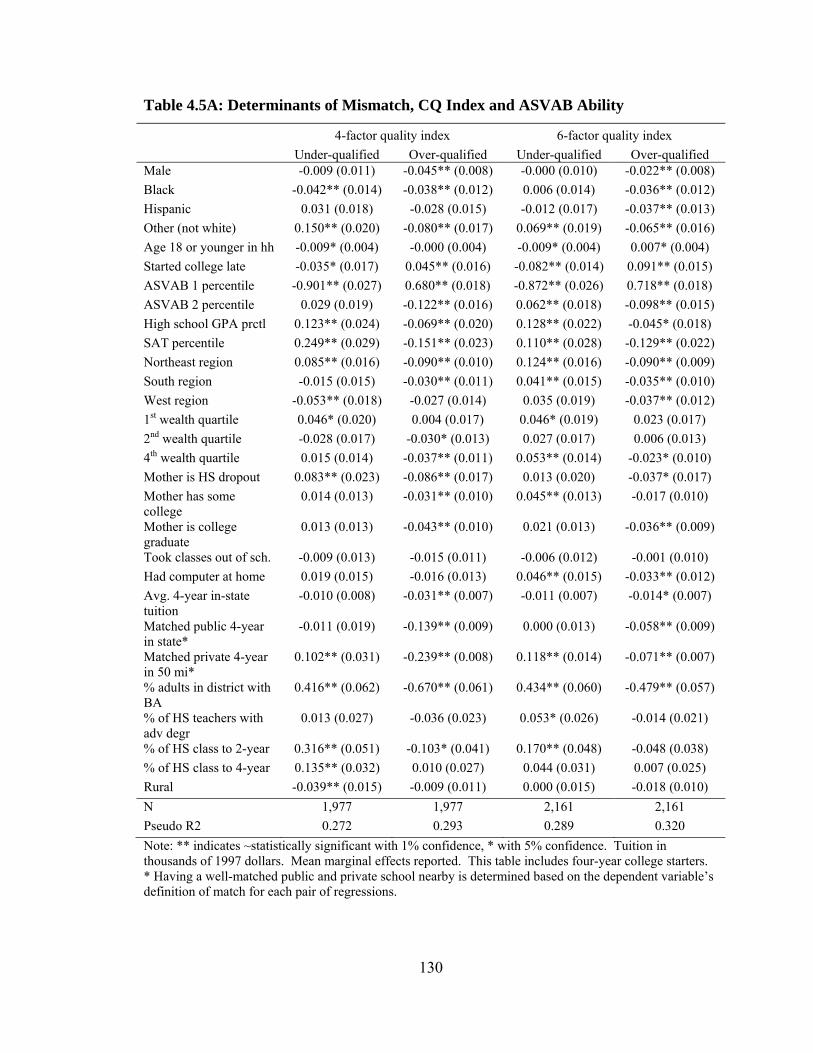
130

Table 4.5A: Determinants of Mismatch, CQ Index and ASVAB Ability

4-factor quality index 6-factor quality index Under-qualified Over-qualified Under-qualified Over-qualified Male -0.009 (0.011) -0.045** (0.008) -0.000 (0.010) -0.022** (0.008)

Black -0.042** (0.014) -0.038** (0.012) 0.006 (0.014) -0.036** (0.012)

Hispanic 0.031 (0.018) -0.028 (0.015) -0.012 (0.017) -0.037** (0.013)

Other (not white) 0.150** (0.020) -0.080** (0.017) 0.069** (0.019) -0.065** (0.016)

Age 18 or younger in hh -0.009* (0.004) -0.000 (0.004) -0.009* (0.004) 0.007* (0.004)

Started college late -0.035* (0.017) 0.045** (0.016) -0.082** (0.014) 0.091** (0.015)

ASVAB 1 percentile -0.901** (0.027) 0.680** (0.018) -0.872** (0.026) 0.718** (0.018)

ASVAB 2 percentile 0.029 (0.019) -0.122** (0.016) 0.062** (0.018) -0.098** (0.015)

High school GPA prctl 0.123** (0.024) -0.069** (0.020) 0.128** (0.022) -0.045* (0.018)

SAT percentile 0.249** (0.029) -0.151** (0.023) 0.110** (0.028) -0.129** (0.022)

Northeast region 0.085** (0.016) -0.090** (0.010) 0.124** (0.016) -0.090** (0.009)

South region -0.015 (0.015) -0.030** (0.011) 0.041** (0.015) -0.035** (0.010)

West region -0.053** (0.018) -0.027 (0.014) 0.035 (0.019) -0.037** (0.012)

1st wealth quartile 0.046* (0.020) 0.004 (0.017) 0.046* (0.019) 0.023 (0.017)

2nd wealth quartile -0.028 (0.017) -0.030* (0.013) 0.027 (0.017) 0.006 (0.013)

4th wealth quartile 0.015 (0.014) -0.037** (0.011) 0.053** (0.014) -0.023* (0.010)

Mother is HS dropout 0.083** (0.023) -0.086** (0.017) 0.013 (0.020) -0.037* (0.017)

Mother has some college

0.014 (0.013) -0.031** (0.010) 0.045** (0.013) -0.017 (0.010)

Mother is college graduate

0.013 (0.013) -0.043** (0.010) 0.021 (0.013) -0.036** (0.009)

Took classes out of sch. -0.009 (0.013) -0.015 (0.011) -0.006 (0.012) -0.001 (0.010)

Had computer at home 0.019 (0.015) -0.016 (0.013) 0.046** (0.015) -0.033** (0.012)

Avg. 4-year in-state tuition

-0.010 (0.008) -0.031** (0.007) -0.011 (0.007) -0.014* (0.007)

Matched public 4-year in state*

-0.011 (0.019) -0.139** (0.009) 0.000 (0.013) -0.058** (0.009)

Matched private 4-year in 50 mi*

0.102** (0.031) -0.239** (0.008) 0.118** (0.014) -0.071** (0.007)

% adults in district with BA

0.416** (0.062) -0.670** (0.061) 0.434** (0.060) -0.479** (0.057)

% of HS teachers with adv degr

0.013 (0.027) -0.036 (0.023) 0.053* (0.026) -0.014 (0.021)

% of HS class to 2-year 0.316** (0.051) -0.103* (0.041) 0.170** (0.048) -0.048 (0.038)

% of HS class to 4-year 0.135** (0.032) 0.010 (0.027) 0.044 (0.031) 0.007 (0.025)

Rural -0.039** (0.015) -0.009 (0.011) 0.000 (0.015) -0.018 (0.010)

N 1,977 1,977 2,161 2,161

Pseudo R2 0.272 0.293 0.289 0.320

Note: ** indicates ~statistically significant with 1% confidence, * with 5% confidence. Tuition in thousands of 1997 dollars. Mean marginal effects reported. This table includes four-year college starters. * Having a well-matched public and private school nearby is determined based on the dependent variable’s definition of match for each pair of regressions.

131

Table 4.5B: Determinants of Mismatch, SAT Mismatch

Under-qualified Over-qualified Male 0.067** (0.007) -0.053** (0.005)

Black -0.110** (0.008) 0.081** (0.010)

Hispanic -0.060** (0.010) -0.026** (0.010)

Other (not white) 0.122** (0.013) 0.004 (0.011)

Age 18 or younger in household -0.021** (0.003) -0.004 (0.003)

Started college late -0.081** (0.012) -0.052** (0.010)

ASVAB 1 percentile 0.012 (0.018) 0.055** (0.015)

ASVAB 2 percentile 0.072** (0.011) -0.033** (0.010)

High school GPA percentile 0.187** (0.013) -0.008 (0.011)

SAT percentile -0.844** (0.018) 0.458** (0.016)

Northeast region -0.008 (0.009) -0.021** (0.007)

South region -0.069** (0.007) -0.028** (0.007)

West region -0.101** (0.009) 0.016 (0.009)

1st wealth quartile 0.160** (0.014) 0.023 (0.012)

2nd wealth quartile 0.048** (0.010) -0.028** (0.008)

4th wealth quartile 0.070** (0.009) -0.040** (0.006)

Mother is HS dropout 0.049** (0.013) -0.094** (0.008)

Mother has some college 0.034** (0.008) -0.083** (0.005)

Mother is college graduate 0.042** (0.008) -0.104** (0.005)

Took classes outside of school 0.042** (0.008) -0.039** (0.006)

Had computer at home -0.003 (0.010) 0.053** (0.010)

Avg. 4-year in-state tuition -0.008 (0.005) 0.005 (0.004)

Matched public 4-year in state* -0.006 (0.022) -0.116** (0.008)

Matched private 4-year in 50 mi* -0.236** (0.009) 0.165** (0.037)

% adults in district with BA 0.293** (0.039) -0.144** (0.034)

% of HS teachers with adv degr -0.163** (0.015) -0.004 (0.013)

% of HS class to 2-year 0.175** (0.030) 0.271** (0.025)

% of HS class to 4-year 0.093** (0.018) 0.028 (0.016)

Rural -0.030** (0.007) 0.047** (0.007)

N 1,177 1,177

Pseudo R2 0.240 0.194

Note: ** indicates ~statistically significant with 1% confidence, * with 5% confidence. Tuition in thousands of 1997 dollars. Mean marginal effects reported. This table includes four-year college starters. * Having a well-matched public and private school nearby is determined based on the dependent variable’s definition of match for each pair of regressions.

132

Table 4.5C: Determinants of Mismatch, CQ Index and ASVAB Ability, All Starters

Ptiles based on 4-year Ptiles based on all Under-qualified Over-qualified Under-qualified Over-qualified Male 0.000 (0.007) -0.021** (0.008) -0.003 (0.007) -0.019* (0.008)

Black 0.038** (0.010) -0.124** (0.010) 0.057** (0.010) -0.117** (0.010)

Hispanic -0.026** (0.009) -0.027* (0.011) -0.001 (0.010) -0.036** (0.011)

Other (not white) 0.081** (0.015) -0.085** (0.015) 0.089** (0.015) -0.066** (0.015)

Age 18 or younger in hh -0.010** (0.003) 0.003 (0.003) -0.004 (0.003) 0.000 (0.003)

Started college late -0.069** (0.007) 0.086** (0.011) -0.076** (0.008) 0.094** (0.011)

ASVAB 1 percentile** -0.448** (0.018) 0.869** (0.018) -0.708** (0.020) 0.826** (0.016)

ASVAB 2 percentile** 0.089** (0.012) -0.125** (0.015) 0.095** (0.013) -0.141** (0.014)

High school GPA prcntl** 0.141** (0.016) -0.163** (0.017) 0.140** (0.016) -0.195** (0.017)

SAT percentile** 0.062** (0.020) -0.247** (0.022) 0.085** (0.021) -0.216** (0.022)

Northeast region 0.112** (0.015) -0.126** (0.011) 0.131** (0.014) -0.091** (0.011)

South region -0.009 (0.010) 0.011 (0.012) -0.036** (0.010) 0.042** (0.012)

West region -0.037** (0.011) -0.016 (0.014) -0.061** (0.011) -0.014 (0.013)

1st wealth quartile 0.004 (0.012) -0.016 (0.013) -0.019 (0.012) -0.000 (0.013)

2nd wealth quartile -0.013 (0.011) 0.007 (0.012) -0.029** (0.011) 0.046** (0.012)

4th wealth quartile 0.029** (0.010) -0.040** (0.010) -0.002 (0.010) -0.026** (0.010)

Mother is HS dropout 0.005 (0.012) -0.066** (0.014) 0.011 (0.012) -0.041** (0.014)

Mother has some college 0.039** (0.009) 0.005 (0.010) 0.033** (0.009) -0.003 (0.009)

Mother is college graduate 0.042** (0.010) -0.076** (0.010) 0.045** (0.010) -0.084** (0.009)

Took classes out of sch. -0.001 (0.009) 0.004 (0.010) -0.005 (0.009) -0.027** (0.009)

Had computer at home 0.034** (0.010) -0.024* (0.011) 0.034** (0.010) -0.023* (0.011)

Avg. 4-year in-state tuition

0.010 (0.006) -0.045** (0.007) -0.006 (0.006) -0.039** (0.007)

Avg. 2-year in-state tuition

-0.053** (0.009) 0.052** (0.010) -0.059** (0.009) 0.031** (0.009)

Matched public 2- or 4-year in state*

-0.061** (0.015) -0.130** (0.017) -0.081** (0.014) -0.131** (0.014)

Matched private 2- or 4-year in 50 mi*

0.054** (0.009) 0.004 (0.009) 0.064** (0.009) -0.012 (0.009)

% adults in district with BA

0.357** (0.040) -0.502** (0.051) 0.412** (0.044) -0.489** (0.049)

% of HS teachers with adv degr

0.040* (0.017) 0.022 (0.020)

0.041* (0.018) -0.000 (0.019)

% of HS class to 2-year -0.180** (0.034) 0.280** (0.035) -0.181** (0.036) 0.212** (0.033)

% of HS class to 4-year 0.012 (0.021) -0.023 (0.024) 0.042 (0.022) -0.049* (0.023)

Rural 0.005 (0.010) -0.001 (0.011) 0.022* (0.011) 0.013 (0.011)

N 3,388 3,388 3,388 3,388

Pseudo R2 0.199 0.285 0.278 0.283

Note: ** indicates ~statistically significant with 1% confidence, * with 5% confidence. Tuition in thousands of 1997 dollars. Mean marginal effects reported. * Having a well-matched public and private school nearby is determined based on the dependent variable’s definition of match for each pair of regressions. ** Percentiles are set by 4-year starters in first two columns and 2- and 4-year starters in last two columns.

133

Figure 4.1: Distribution of College Mismatch

Mismatch defined as student ability percentile - college quality percentile. Histogram includes estimated kernel density distribution.

134

Table A4.1: The Sample

Total Observations 8,984

Graduated HS 7,052

Did not graduate HS but got GED 757

Started at a 2-year college* 2,467

Started at a 4-year college 2,771

Starting college qualities

Of quality quartile 1 1,444

Of quality quartile 2 1,347

Of quality quartile 3 917

Of quality quartile 4 900

Missing quality 630

Has quality, but missing ability 780

Starting college qualities, 4-year only

Of quality quartile 1 614

Of quality quartile 2 602

Of quality quartile 3 582

Of quality quartile 4 507

Missing quality 466

Has quality, but missing ability 328

* The 2-year starters include 17 respondents who have no record of either graduating high school or getting a GED. College quality for first college attended. For 4-year schools only this is based on the 4-factor college quality measure. For all colleges it’s based on the 6-factor college quality. Of the 203 respondents who started at a 2-year school for which we don’t have a quality measure, 65 are missing quality because I could not identify the college and 237 are missing quality because the school was not in IPEDS or did not have enough information to make the quality measure. For 310 4-year schools without quality, 39 had no identifier and 271 did not have all the quality measures.

135

Table A4.2: Description of Independent Variables

Variable Description Male

Dummy variable equal to 1 if the respondent is male, 0 otherwise Black Dummy variable equal to 1 if the respondent lists black as a racial category, 0

otherwise Hispanic Dummy variable equal to 1 if the respondent lists Hispanic as an ethnic category and

doesn’t list black as a racial category Started college late

Equal to one if the respondent started college more than 12 months after graduating high school.

Region of the U.S. Region where the respondent lived in the fall before they graduated high school.

ASVAB percentile Described in the data appendix High School GPA Collected from the respondent’s high school transcript and standardized to a 4-point

scale weighted by Carnegie credits. GPA percentile is calculated within our [weighted] sample of college-goers in the same way as the ASVAB percentile.

SAT score The combined score on the math and verbal section of the SAT (max score 1600), collected from the respondent’s high school transcript. SAT percentile is calculated within our [weighted] sample of college-goers in the same way as the ASVAB percentile.

Mother’s Education

The respondent’s mother’s self-reported highest grade completed. This measure is taken from the NLS-constructed household roster for the fall before the respondent graduated high school (or earlier if that year is unavailable). Mother refers to the mother figure that the respondent lived with. When there was more than one mother figure included in the household, we considered only one, using the following prioritization: biological, adopted, step, or foster.

Took classes outside of school

From the 1997 youth survey. Equal to one if he or she answered yes to “In a typical week, did you spend any time taking extra classes or lessons for example, music, dance, or foreign language lessons?”

Had computer at home

From the 1997 youth survey. Equal to one if he or she answered yes to “In the past month, has your home usually had a computer?”

Had dictionary at home

From the 1997 youth survey. Equal to one if he or she answered yes to “In the past month, has your home usually had a dictionary?”

Quality percentile of state flagship

Quality percentile, as described in the data appendix, of the flagship state university in the state where the respondent lived in the fall before they graduated high school.

% in census district with BA

The share of the adult (over 25) population that has at least 4 years of college (from 1990 census) in the census district where the respondent lived in 1997.

Household income Total 1996 household income for the household where the respondent lived in 1997. This number is taken from the parent survey where available and from the youth survey when the parent response is missing (98.6% from parent survey). We use total income across everyone living in the same household as the respondent (whether or not respondent is independent from parents in 1997). Income quintile cutoffs are taken from the 1996 Current Population Survey Annual Social and Economic Supplement Income Percent Distribution for Families.

Household wealth Total 1997 household net worth for the household where the respondent lived in 1997. This number is taken from the parent survey where available and from the youth survey when the parent response is missing (98.6% from parent survey). We use total wealth across everyone living in the same household as the respondent (whether or not respondent is independent from parents in 1997). 1997 wealth quartiles are calculated within the (weighted) sample.

136

Table A4.3: Description of Independent Variables, Continued

% of HS teachers with advanced degrees

From the restricted NLSY97 School Survey. The response from the respondent’s last high school to the survey question “what percent of your teachers have more than a bachelor degree?”

% of HS class to 4-year

From the restricted NLSY97 School Survey. The response from the respondent’s last high school to the survey question “by the fall following graduation, about what percent of your 1999 graduating class enrolled in a 4-year college?”

In-state tuition at flagship

In-state tuition, by year, for the flagship university of each state is from the State of Washington Higher Education Coordinating Board. “In-state” tuition for District of Columbia residents is calculated as max(national average in-state tuition, national average out-of-state tuition - $10,000) in accordance with DC Tuition Assistance Grant Program. For each respondent, in-state tuition is the in-state tuition in the fall before they graduated high school in the state where they lived that fall. All tuition is CPI-deflated to 1997 dollars.

Rural Indicates that the respondent did not live within a Metropolitan Statistical Area (MSA) in fall before they graduated high school.

Nearby universities

Distance is calculated from the zipcode of the respondent’s residence in the fall before they graduated from high school. In the 352 cases where the zipcode that fall was missing, the zipcode from the last available year prior to graduation is used.

137

References Alon, Sigal and Marta Tienda (2005): “Assessing the ‘Mismatch’ Hypothesis: Differences in College Graduation Rates by Institutional Selectivity,” Sociology of Education, 78(4), pp. 294-315. Arcidiacono, Peter (2004): “Ability Sorting and the Returns to College Major,” Journal of Econometrics, 121, pp. 343 – 375. Arcidiacono, Peter, Esteban Aucejo, Hanming Fang, and Kenneth Spenner (2011): “Does Affirmative Action Lead to Mismatch? A New Test and Evidence,” Duke Working Paper. Arulampalam, Wiji, Robin Naylor, and Jeremy Smith (2005): “Effects of In-Class Variation and Student Rank on the Probability of Withdrawal: Cross-Section and Time-Series Analysis for UK University Students,” Economics of Education Review, 24, pp. 251-262. Avery, Christopher and Sarah Turner (2009): “Playing the College Application Game: Critical Moves and the Link to Socio-Economic Circumstances,” University of Virginia Working Paper. Black, Daniel and Jeffrey Smith (2004): “How Robust is the Evidence on the Effects of College Quality? Evidence from Matching,” Journal of Econometrics, 121(1), pp. 99-124. Black, Daniel and Jeffrey Smith (2006): “Evaluating the Returns to College Quality with Multiple Proxies for Quality,” Journal of Labor Economics, 24(3), pp. 701-728. Bowen, William, Matthew Chingos, and Michael McPherson (2009): Crossing the Finish Line: Completing College at America’s Public Universities, Princeton, PA: Princeton University Press. Brand, Jennie, and Yu Xie (2010): “Who Benefits Most from College? Evidence for Negative Selection in Heterogeneous Economic Returns to Higher Education,” American Sociological Review, 75, pp. 273–302. Bound, John, Michael Lovenheim, and Sarah Turner (2007): "Understanding the Decrease in College Completion Rates and the Increased Time to the Baccalaureate Degree," PSC Research Report No. 07-626. Cawley, John, James Heckman, and Edward Vytlacil (2001): “Three Observations on Wages and Measure Cognitive Ability,” Labor Economics, 8(4), pp. 419-442. College Board (2008): Trends in Student Aid 2008, New York: College Board Publications. Dale, Stacy and Alan Krueger (2002): "Estimating The Payoff To Attending A More Selective College: An Application Of Selection On Observables And Unobservables," Quarterly Journal of Economics, 117(4), pp. 1491-1527. Dale, Stacy and Alan Krueger (2011): “Estimating the Return to College Selectivity over the Career Using Administrative Earning Data,” Princeton University Industrial Relations Section Working Paper #563. Dillon, Eleanor and Jeffrey Smith (2012): “The Consequences of Mismatch between Student Ability and College Quality,” University of Michigan Manuscript. Goldin, Claudia and Lawrence Katz (2008): The Race between Education and Technology. Cambridge, MA: Harvard University Press. Griffith, Amanda and Donna Rothstein (2009): "Can't Get Here from There: The Decision to Apply to a Selective Institution," Economics of Education Review, 28(5), pp. 620-628.

138

Howell, Jessica (2010): “Assessing the Impact of Eliminating Affirmative Action in Higher Education,” California State University, Sacramento Working Paper. Hoxby, Caroline (2009): "The Changing Selectivity of American Colleges," Journal of Economic Perspectives, 23(4), pp. 95-118. Johnson, William (2006): “Hours Constraints In Market Equilibrium,” University of Virginia Working Paper. Johnson, William (2008): “Hours Constraints Are Partially Illusory,” University of Virginia Working Paper. Kane, Thomas and Christopher Avery (2004): “Student Perceptions of College Opportunities: The Boston COACH Program,” in Caroline Hoxby (ed.) College Choices: The Economics of Where to Go, When to Go, and How to Pay for It, Chicago: University of Chicago Press. Krueger, Alan, Jesse Rothstein, and Sarah Turner (2006): “Race, Income, and College in 25 Years: Evaluating Justice O’Connor’s Conjecture,” American Law and Economics Review, 8(2), pp. 282–311. Light, Audrey and Wayne Strayer (2000): “Determinants of College Completion: School Quality or Student Ability?” Journal of Human Resources, 35(2), pp. 299-332. Neal, Derek and William Johnson (1996): “The Role of Premarket Factors in Black-White Wage Differences,” Journal of Political Economy, 104(5), pp. 869-895. Reynolds, C. Lockwood (2009): "Where to Attend? Estimates of the Effects of Beginning College at a Two-year Institution," Kent State University Working Paper.