three essays on an emerging financial market
TRANSCRIPT

Clemson UniversityTigerPrints
All Dissertations Dissertations
5-2018
Three Essays on an Emerging Financial MarketYuekai ChengClemson University, [email protected]
Follow this and additional works at: https://tigerprints.clemson.edu/all_dissertations
This Dissertation is brought to you for free and open access by the Dissertations at TigerPrints. It has been accepted for inclusion in All Dissertations byan authorized administrator of TigerPrints. For more information, please contact [email protected].
Recommended CitationCheng, Yuekai, "Three Essays on an Emerging Financial Market" (2018). All Dissertations. 2160.https://tigerprints.clemson.edu/all_dissertations/2160

Three Essays on an Emerging Financial Market
A DissertationPresented to
the Graduate School of Clemson University
In Partial Fulfillmentof the Requirements for the Degree
Doctor of PhilosophyEconomics
Accepted by:Dr. Gerald P. Dwyer, Jr., Committee Chair
Dr. Michal M. JerzmanowskiDr. Sergey MityakovDr. Robert F. Tamura
byYuekai Cheng
May 2018

Abstract
This dissertation examines the impact of retail trading, price limit rule and market
opening on the Chinese stock market. The Chinese stock market is the second largest
in the world based on market capital. In addition, it has a daily average turnover
eight times of the US stock market. It also has a price limit rule which limits its
daily fluctuation. Furthermore, retail investors play an important role in the Chinese
stock market, meaning its investor structure is different from that of developed stock
markets.
In the first chapter, I explore the impact of the breadth of ownership on stock
returns and turnovers in the Chinese A share market. Using data in the period of
2002-2017, I find that firms with a higher breadth of ownership and a higher change
in the breadth of ownership have lower returns and higher average daily turnovers
in the subsequent quarter. Furthermore, firms with a higher breadth of ownership
have a stronger reversal effect in returns and a stronger negative relationship be-
tween turnovers and subsequent returns. Moreover, adding the breadth and the
change of breadth factors to a six-factor model improves the explanatory power of
excess returns, this improvement is mainly provided by the change of breadth factor.
These findings are consistent with the hypothesis that retail investors are attention-
motivated traders and their trading behavior causes overreaction and mispricing in
the Chinese stock market.
In the second chapter, I explore the impact of the Chinese price limit policy on
ii

long-term stock performance using IPOs on the A share market and HKEx market
from 2006 to 2015. I use a difference-in-differences method to investigate whether
a new IPO policy for the A share market causing consecutive limit-ups on the first
several trading days after the IPO has a long-term effect on stock return, turnover,
volatility and β coefficient. The empirical results are consistent with the hypothesis
that this price limit policy causes the IPO firms on the A share market to have higher
stock returns, turnovers, volatility and β coefficients over a 2-years period after the
IPO.
In the last chapter, I explore the influence of Hong Kong investors on stock returns
and turnovers of stocks involved in the Shanghai-Hong Kong Stock Connect policy.
Using data from 2014-2016 in the Chinese stock market, I find that stocks dual-listed
in Shanghai and Hong Kong have higher monthly stock returns than stocks involved
in the Shanghai-Hong Kong stock connect but listed only in Shanghai; however, the
difference in stock returns between the dual-listed and other Shanghai Hong Kong
stock connect involved stocks decreases gradually. Moreover, stocks dual-listed in
Shanghai and Hong Kong have higher daily average turnovers than stocks involved
in the Shanghai-Hong Kong stock connect but listed only in Shanghai, and the dif-
ference in daily average turnover between dual-listed and other Shanghai-Hong Kong
stock connect involved stocks decreases gradually. These empirical results are consis-
tent with the hypothesis that Hong Kong investors were initially more likely to buy
Shanghai-Hong Kong dual-listed stocks through the stock connect channel; however,
iii

they extended their investment target to stocks involved in the stock connect but
listed only in Shanghai after they gained experience and became familiar with the
Shanghai stock market.
iv

Acknowledgement
I own many more debts than I can possibly acknowledge. I thank my advicer, Gerald
P. Dwyer, Jr., for his guidance on my research and comments on my dissertation.
I also thank my committee members, Michal M. Jerzmanowski, Sergey Mityakov,
Robert F. Tamura, for the comments and advice on my research. Thanks are also
due to Aspen Gorry, whose comments in macro workshop led me to write an essay
on stock market opening. I am grateful to my master advicer, Yao Zheng for his
guidance and support on my research and career development. I thank my teacher,
Xu Weidong for his advice on my research and his help in providing data. I am
grateful to Barbara J. Ramirez for helping me in English writing. I thank my room-
mates, Wu Xiaosong, Zhou Jian and Zou Pengfei, and my classmates, Fan Haobin,
He Qiwei, Tian Chuan, Wang Chen, Wei Qing and Huang Yiheng, who are all my
good friends. Five years study with you are wonderful and unforgettable experience
for me. Thanks also go to my foreign friends, Madeleine Nelson, Jonathan Ernest,
Kelsey Roberts, Leah Kitashima, Smriti Bhargava, Maria Droganova, Richard Sessa
and Corbin Fuller. We have so much fun together. I thank Zhao Liping for every-
thing we have experienced together in the last seven years, including applying for
Economics PhD, doing research, exploring trading strategies, learning programming
languages. Last, certainly not least, I owe more than I can say to the support and
love of my parents.
v

Contents
1 The Breadth of ownership, turnovers and stock returns in the Chi-
nese stock market 1
1.1 Introduction . . . . . . . . . . . . . . . . . . . . . . . . . . . . . . . . 1
1.2 The Hypotheses . . . . . . . . . . . . . . . . . . . . . . . . . . . . . . 7
1.3 The Data and Variables . . . . . . . . . . . . . . . . . . . . . . . . . 11
1.4 Empirical Results . . . . . . . . . . . . . . . . . . . . . . . . . . . . . 21
1.4.1 Determinants of the Breadth of Ownership . . . . . . . . . . . 21
1.4.2 Breadth of Ownership and Stock Returns . . . . . . . . . . . . 25
1.4.3 Breadth of Ownership and Turnovers . . . . . . . . . . . . . . 36
1.4.4 Breadth of Ownership and the Reversal Effect . . . . . . . . . 42
1.4.5 Breadth of Ownership and Turnover–Return Relation . . . . . 44
1.4.6 Breadth of ownership and factor model . . . . . . . . . . . . . 46
1.5 Summary and Conclusions . . . . . . . . . . . . . . . . . . . . . . . . 56
1.6 Appendix . . . . . . . . . . . . . . . . . . . . . . . . . . . . . . . . . 56
1.6.1 A Model of the Breadth of Ownership, Turnover and Stock
Returns . . . . . . . . . . . . . . . . . . . . . . . . . . . . . . 56
1.6.2 Comparison of the Breadth of Ownership Among Feature Groups 60
1.6.3 Test of Reversal Effect . . . . . . . . . . . . . . . . . . . . . . 63
1.6.4 Test of Turnover–Return Relationship . . . . . . . . . . . . . . 65
vi

2 Price Limit Rule and Long-term Performance of IPO in the Chinese
Stock Market 67
2.1 Introduction . . . . . . . . . . . . . . . . . . . . . . . . . . . . . . . . 67
2.2 the Hypothesis . . . . . . . . . . . . . . . . . . . . . . . . . . . . . . 70
2.3 The Data and Variables . . . . . . . . . . . . . . . . . . . . . . . . . 72
2.4 Long-Term Performance of the IPO . . . . . . . . . . . . . . . . . . . 83
2.4.1 Performance by month . . . . . . . . . . . . . . . . . . . . . . 83
2.4.2 Long-term performance by IPO year . . . . . . . . . . . . . . 103
2.4.3 Regression Analysis . . . . . . . . . . . . . . . . . . . . . . . . 112
2.5 Summary and Conclusions . . . . . . . . . . . . . . . . . . . . . . . . 123
3 Do Investors Invest in Familiarity? Evidence from the Shanghai-
Hong Kong Stock Connect 125
3.1 Introduction . . . . . . . . . . . . . . . . . . . . . . . . . . . . . . . . 125
3.2 the Hypotheses . . . . . . . . . . . . . . . . . . . . . . . . . . . . . . 129
3.3 The Data and Variables . . . . . . . . . . . . . . . . . . . . . . . . . 130
3.4 Empirical Results . . . . . . . . . . . . . . . . . . . . . . . . . . . . . 137
3.5 Summary and Conclusions . . . . . . . . . . . . . . . . . . . . . . . . 147
vii

List of Tables
1 Descriptive Statistics . . . . . . . . . . . . . . . . . . . . . . . . . . . 16
2 Correlation Analysis . . . . . . . . . . . . . . . . . . . . . . . . . . . 19
3 Determinants of Breadth of Ownership . . . . . . . . . . . . . . . . . 23
4 Return Comparison for Stocks with Different Breadth of Ownerships 29
5 Return Comparison for Stocks with Different Change of Breadth of
Ownership . . . . . . . . . . . . . . . . . . . . . . . . . . . . . . . . . 30
6 Regression Results of Subsequent Returns on Breadth of Ownership . 34
7 Turnover Comparison for Stocks with Different Breadth of Ownership 37
8 Regression Results of Subsequent Turnovers on Breadth of Ownership 40
9 Reversal Effect, Turnover-Return Relation and Breadth of Ownership 43
10 Descriptive Statistics and Correlation Analysis of Factors . . . . . . . 48
11 Regression of Factors on Other Factors (Equally Weighted Factor Re-
turns) . . . . . . . . . . . . . . . . . . . . . . . . . . . . . . . . . . . 49
12 Regression of Factors on Other Factors (Value Weighted Factor Returns) 50
13 Test of Factor Models . . . . . . . . . . . . . . . . . . . . . . . . . . . 54
14 Test of Factor Models . . . . . . . . . . . . . . . . . . . . . . . . . . . 55
15 Comparison of Breadth of Ownership for Different Feature Groups . . 61
16 Comparison of Change of Breadth of Ownership for Different Feature
Groups . . . . . . . . . . . . . . . . . . . . . . . . . . . . . . . . . . . 62
17 Return Comparison for Stocks with Different Current Returns . . . . 64
viii

18 Return Comparison for Stocks with Different Current Turnovers . . . 65
19 The Distribution of Sectors for the IPO firms . . . . . . . . . . . . . 73
20 Descriptive Statistics . . . . . . . . . . . . . . . . . . . . . . . . . . . 75
21 Long term performance of IPO . . . . . . . . . . . . . . . . . . . . . 80
22 Mean of cumulative abnormal return after IPO (Composite index) . . 84
23 Median of cumulative abnormal return after IPO (Composite index) . 86
24 Mean of cumulative abnormal return after IPO (SmallCap index) . . 87
25 Median of cumulative abnormal return after IPO (SmallCap index) . 89
26 Mean of adjusted turnover after IPO (Composite index) . . . . . . . . 91
27 Median of adjusted turnover after IPO (Composite index) . . . . . . 93
28 Mean of adjusted volatility after IPO (Composite index) . . . . . . . 95
29 Median of adjusted volatility after IPO (Composite index) . . . . . . 98
30 Mean of adjusted volatility after IPO (SmallCap index) . . . . . . . . 100
31 Median of adjusted volatility after IPO (SmallCap index) . . . . . . . 101
32 Two-year cumulative adjusted stock return after the IPO (Composite
index) . . . . . . . . . . . . . . . . . . . . . . . . . . . . . . . . . . . 103
33 Two year cumulative adjusted stock return after IPO (SmallCap index) 105
34 Two year average adjusted daily turnover after IPO (Composite index) 106
35 Two year adjusted daily volatility after IPO (Composite index) . . . 107
36 Two year adjusted daily volatility after IPO (SmallCap index) . . . . 108
37 Two year β coefficient after IPO (Composite index) . . . . . . . . . . 109
ix

38 Two year β coefficient after IPO (SmallCap index) . . . . . . . . . . 111
39 Price limit and stock return . . . . . . . . . . . . . . . . . . . . . . . 113
40 Price limit and β coefficient . . . . . . . . . . . . . . . . . . . . . . . 116
41 Price limit and daily volatility . . . . . . . . . . . . . . . . . . . . . . 118
42 Price limit and daily turnover . . . . . . . . . . . . . . . . . . . . . . 121
43 Descriptive Statistics Before Winsorizing . . . . . . . . . . . . . . . . 134
44 Descriptive Statistics After Winsorizing . . . . . . . . . . . . . . . . . 136
45 Impact of Shanghai Hong Kong Stock Connect on Stock Returns and
Turnovers . . . . . . . . . . . . . . . . . . . . . . . . . . . . . . . . . 138
46 Mean of monthly returns after enactment of Shanghai Hong Kong
Stock Connect . . . . . . . . . . . . . . . . . . . . . . . . . . . . . . . 142
47 Mean of 5 month returns after enactment of Shanghai Hong Kong
Stock Connect . . . . . . . . . . . . . . . . . . . . . . . . . . . . . . . 144
48 Mean of monthly turnovers after enactment of Shanghai Hong Kong
Stock Connect . . . . . . . . . . . . . . . . . . . . . . . . . . . . . . . 146
49 Mean of 5 month turnovers after enactment of Shanghai Hong Kong
Stock Connect . . . . . . . . . . . . . . . . . . . . . . . . . . . . . . . 148
x

List of Figures
1 Mean of cumulative abnormal return after IPO (Composite index) . . 83
2 Median of cumulative abnormal return after IPO (Composite index) . 85
3 Mean of cumulative abnormal return after IPO (SmallCap index) . . 88
4 Median of cumulative abnormal return after IPO (SmallCap index) . 88
5 Mean of adjusted turnover after IPO (Composite index) . . . . . . . . 90
6 Median of adjusted turnover after IPO (Composite index) . . . . . . 94
7 Mean of adjusted volatility after IPO (Composite index) . . . . . . . 96
8 Median of adjusted volatility after IPO (Composite index) . . . . . . 99
9 Mean of adjusted volatility after IPO (SmallCap index) . . . . . . . . 99
10 Median of adjusted volatility after IPO (SmallCap index) . . . . . . . 102
11 Two year cumulative adjusted stock return after IPO (Composite index)103
12 Two year cumulative adjusted stock return after IPO (SmallCap index) 104
13 Two year average adjusted daily turnover after IPO (Composite index) 105
14 Two year adjusted daily volatility after IPO (Composite index) . . . 107
15 Two year adjusted daily volatility after IPO (SmallCap index) . . . . 109
16 Two year β coefficient after IPO (Composite index) . . . . . . . . . . 110
17 Two year β coefficient after IPO (SmallCap index) . . . . . . . . . . 111
18 Mean of monthly returns after enactment of Shanghai Hong Kong
Stock Connect . . . . . . . . . . . . . . . . . . . . . . . . . . . . . . . 143
xi

19 Mean of 5 month returns after enactment of Shanghai Hong Kong
Stock Connect . . . . . . . . . . . . . . . . . . . . . . . . . . . . . . . 144
20 Mean of monthly turnovers after enactment of Shanghai Hong Kong
Stock Connect . . . . . . . . . . . . . . . . . . . . . . . . . . . . . . . 147
21 Mean of 5 month turnovers after enactment of Shanghai Hong Kong
Stock Connect . . . . . . . . . . . . . . . . . . . . . . . . . . . . . . . 148
xii

1 The Breadth of ownership, turnovers and stock
returns in the Chinese stock market
1.1 Introduction
An emerging market, the Chinese stock market is the second largest in the world
based on its market value, with a transaction volume in 2015 38% of the total volume
of the world stock market. From December 1990, the day the Chinese stock market
was founded, to November 2017, the Shanghai Composite index increased by 3271%,
and the average annual return is 13.98%. During the same period, the Dow Jones
Industry Average increased by 795%, with an average annual return of 8.50%. The
daily average turnover of the Chinese stock market is about 8 times of the US stock
market.
An important reason that the Chinese stock market has different patterns in stock
returns and turnovers than the developed markets is the high fraction of retail traders
in the Chinese stock market. In contrast to developed markets in which institutional
investors play a major role, the Chinese stock market is significantly affected by the
behavior of retail investors. For example, at the end of the third quarter of 2014,
households and institutional investors, held 33% and 44%, respectively, of the shares
in the US stock market, while at the end of the third quarter of 2015 in the Chinese
A share market, by contrast, retail investors and institutional investors held 42% and
7%, respectively, of the tradable shares.
In this paper, I explore the impact of the breadth of ownership (the number of
1

shareholders per 1 million Chinese Yuan of market value) and the change of the
breadth of ownership (the quarterly percentage change of the number of sharehold-
ers) on stock returns and turnovers, obtaining implications of the asset pricing in the
Chinese stock market. Using data from the period 2002-2017, I find that firms with a
higher breadth of ownership and a higher percentage change of the breadth of owner-
ship have lower returns and higher average daily turnovers in the subsequent quarter.
Furthermore, firms with a higher breadth of ownership have a stronger reversal effect
in returns and a stronger negative relationship between turnovers and subsequent re-
turns. Moreover, adding the breadth and the change of breadth factors to a six-factor
model improves the explanatory power of excess returns, this improvement mainly
being provided by the change of breadth factor. These findings are consistent with
the hypothesis that retail investors are attention-motivated traders and their trading
behavior results in overreactions and mispricings in the Chinese stock market.
Factor pricing models assume that the stock market is efficient, so stock returns
covary with factors which proxy for common risks. After both Sharpe (1964) and
Lintner (1965) found that excess market return is a factor in asset pricing, addi-
tional research found book to market equity ratio and size (Fama and French, 1993),
momentum (Carhart, 1994), liquidity (Pastor, Stambaugh, 2003), investment and
profitability (Hou, Xue, and Zhang, 2012; Fama and French, 2015) were documented
as new pricing factors.
The impact of retail trading, which leads to market inefficiency, is ignored in
2

the traditional assets pricing models. Empirical evidence in this paper shows that
adding two factors mimicking portfolios formed by the breadth of ownership and
the change of the breadth of ownership to a six-factor model (Fama, French five
factors and momentum factor) improves the explanatory power of excess returns, an
improvement primarily provided by the change of breadth factor.
Currently, research is simultaneously identifying new factors and discovering anoma-
lies. While size (Banz, 1981), price earnings ratio (Basu, 1977), leverage (Bhandari,
1988), book market ratio (Fama and French, 1992), profitability (Novy-Marx, 2013)
and cash flow (Sloan, 1996) have been proposed as anomalies that challenge the
CAPM and other factor models, there is evidence that improved multi-factor models
can explain these characteristics (Fama and French,1996; Fama and French, 2016).
In this paper, I find that firms with a higher breadth of ownership and a higher
change of the breadth of ownership have lower subsequent returns after controlling
for other firm characteristics for cross-sectional stock returns, and the influence of
the breadth of ownership and the change of the breadth of ownership on future stock
returns cannot be explained by a six-factor model including Fama and French’s five
factors and the momentum factor.
The interplay between market factors and anomalies reflects the inconsistent re-
sults found for market efficiency. There is evidence that factors like book market ratio
(Chen, 2017) cannot proxy for common risk, meaning stock returns reflect firms’ dif-
ferent characteristics (Daniel and Titman, 1997). Additionally, behavioral factors,
3

for instance, irrational expectations (Lakonishok, Shleifer and Vishny, 1994; Brun-
nermeier and Nagel, 2004; Kogan, Ross, Wang and Westerfield, 2006), institutional
trading behavior (O’Brien and Bhushan, 1990; Keim and Madhavan, 1995; Sias and
Starks, 1997; Hotchkiss and Strickland, 2003; Sias, Starks and Titman, 2006), asym-
metric information (Meulbroek, 1992, Coval and Moskowitz, 1999), sentiment (Baker
and Wurgler, 2006; Baker and Wurgler, 2007; Tetlock, 2007), difference in opinion
(Yu, 2001; Diether, Malloy and Scherbina, 2002), and institution factors such as the
short sale constraint (Miller, 1977; Asquith, Patak and Ritter, 2005; Nagel, 2005;
Boehmer, Huszar and Jordan, 2010) are linked to stock returns.
To be specific, there is much research on the behavior of retail investors. Retail
investor ownership (Brandt, Brav, Graham and Kumar, 2010), sentiment (Kaniel,
Saar and Titman, 2008), overconfidence (Barber and Odean, 2000), attention (Bar-
ber and Odean, 2008), disposition effect (Shapira and Venezia, 2001) and visibility
(Gervais, Kaniel and Mingelgrin, 2001) have an impact on stock performance and on
the return of the retail investors themselves.
In this paper, I examine the breadth of ownership of retail investors and treat
the breadth of ownership as a proxy for overreaction and, thus, overpricing given
that there is a strong short sale constraint and retail investors play a significant
role in the Chinese stock market. The negative breadth-return relationship is, thus,
consistent with the hypothesis that irrational retail trading causes overreactions and
overpricings, both of which will be corrected in the future.
4

A firm’s visibility to investors measured by advertising expenditures is positively
related with the breadth of ownership of both individual and institutional investors
(Grullon, Kanatas and Weston, 2004). An increase in the breadth of ownership of
individual investors resulting from a reduction in the minimum trading unit improves
liquidity and is positively related with future stock returns (Amihud, Mendelson and
Uno, 1999). There is also contradicting evidence that an increase in the ownership
breadth of retail investors is a signal of overpricing and a predictor of low returns
(Choi, Jin and Yan, 2013).
The breadth of ownership among institutional investors is negatively related with
differences in opinion and a short sale constraint, meaning that the breadth of own-
ership of institutional investors is positively related with future stock returns (Chen,
Hong and Stein, 2002); Choi, Jin and Yan, 2013). However, the breadth of owner-
ship of institutional investors is positively related to investor recognition; therefore,
the breadth of ownership is negatively related with future stock returns (Lehavy and
Sloan, 2008). The compromising view suggests that the relationship between the
ownership breadth of institutional investors and return can be either positive or neg-
ative depending on the relative strength of the two offsetting forces of disagreement
and sentiment (Cen, Lu and Yang, 2013).
There is significant disagreement among the empirical results on the breadth-
return relationship. The results in this paper are consistent with those of Choi, Jin
and Yan (2013) which also use the Chinese stock market for their data.
5

There is a long-term negative relationship (De Bondt and Thaler, 1985) and a
short-term positive relationship (Jegadeesh and Titman, 1993) between current stock
returns and future stock returns. This paper provides evidence that there is a strong
reversal effect on quarterly stock returns, results that are consistent with De Bondt
and Thaler (1985). Furthermore, I find that firms with a higher breadth of ownership
have a stronger reversal effect. A potential explanation for this result is that firms
with higher ownership breadth have higher retail holdings and, thus, more intense
overreactions to news, meaning that there will be a higher correction in the stock
price.
Stock returns and turnovers are determined by the same firm characteristics in
the same direction (Rouwenhorst, 1999), correlate contemporaneously (Morgan, 1976;
Rogalski, 1978) and react to announcements in the same direction (Bamber and
Cheon, 1995). Dispersion of expectations (Comiskey, Walkling and Weeks, 1987),
risk, size, price, trading costs and S&P 500 membership (Lo and Wang, 2000) affect
turnovers.
After controlling for other potential determinants of cross-sectional turnovers, I
find that firms with a higher breadth of ownership and a higher change of the breadth
of ownership have higher average daily turnovers in the subsequent quarter. Firms
with a higher breadth of ownership are more intensively held by retail investors.
Therefore, the positive breadth-turnover relationship indicates that retail investors
have a higher trading frequency.
6

There is a negative relationship between turnovers and subsequent stock returns
(Datar, Naik and Radcliffe, 1998; Hu, 1997), but other evidence such as a positive
relationship (Claessens et al, 1998) and no relationship (Rouwenhorst, 1999) have also
been documented. This paper shows that there is a negative relationship between
turnovers and subsequent stock returns, a finding which consistent with Datar, Naik
and Radcliffe (1998) and Hu (1997). Firms with a higher breadth of ownership have a
stronger negative relationship between returns and prior turnovers, providing evidence
that irrational retail tradings cause higher turnovers and overpricing.
In conclusion, the findings in this paper are consistent with the hypothesis that
retail investors are attention-motivated traders and their trading behavior leads to
overreaction and overpricing in the Chinese stock market.
Section 2 presents the hypothesis, Section 3 the descriptive statistics of the data
and the variables, while Section 4 examines the impact of the breadth of ownership
on stock returns and turnovers, and Section 5 concludes.
1.2 The Hypotheses
This research tests eight hypotheses. Since institutional investors and retail investors
are the major players in the Chinese stock market, their trading behavior has an
impact on stock prices. In this paper, I assume that institutional investors have
an information advantage and better analytical skills than the retail investors. As
they are information-motivated traders, they buy undervalued stocks, holding them
for an extended period of time. As a result, institutional trading can increase the
7

information content in the stock price. In contrast, because retail investors do not
have an information advantage nor sufficient analytical skills, they are attention-
motivated traders, buying popular stocks which they hold for a short period. As a
result, these retail traders add noise to stock prices. These investors create pricing
errors in the market which are corrected by institutional investors. If a firm has a
larger number of retail investors, then the stock price is likely to be overvalued, and
it will see a lower return. Thus, I hypothesize that
H1: The level of the breadth of ownership is negatively related to subsequent stock
returns.
For the purpose of this research, the breadth of ownership is considered as a metric
of the number of retail investors. Since the Chinese stock market is highly short sale
constrained, most investors can only hold long positions. Only a small fraction of
stocks are allowed to be short sold and only investors with more than 500 thousand
Chinese Yuan of assets in their stock accounts can short sell stocks. As a result, the
total market value of short sold stocks is only 0.008% of the total market value of
the Chinese stock market. An increase in the number of retail investors results in
overreaction to good news, meaning the stock becomes overvalued. In contrast, a
decrease in the number of retail investors indicates that shares are flowing from retail
investors to institutional investors, meaning the stock might be undervalued. There-
fore, the prices of overvalued or undervalued stocks will return to the fundamental in
the future due to institutional tradings. Therefore, I hypothesize that
8

H2: The change in the breadth of ownership is negatively correlated to subsequent
stock returns.
If a firm has a large number of retail investors, then the stock tends to overreact
to both good and bad news. Since this overreaction to information will be corrected
in the future, I hypothesize that
H3: The level of the breadth of ownership is positively correlated to the reversal
effect in stock returns.
The trading behavior of retail investors is more speculative than that of institu-
tional investors. Thus, it is likely that institutional investors exhibit longer holding
periods than retail investors. Therefore, the fraction of shares held by retail investors
affects turnover. Hence, I hypothesize that
H4: Stocks with a higher breadth of ownership have higher subsequent turnovers.
Further, because retail trading is motivated by the attention to popular stocks,
these investors tend to sell their holdings quickly. Consequently, an increase in retail
holdings causes pressure on future stock prices. In contrast, institutional trading is
based on information, and institutional investors often change their positions gradu-
ally, holding them for a long time. Because the increase in institutional holdings is
indicative of less selling pressure and more buying pressure in the future, I hypothesize
that
H5: Stocks with a higher change of the breadth of ownership have higher turnovers.
Past research has found a negative relationship between turnovers and subsequent
9

stock returns. Stocks with higher retail holdings are subject to more irrational trad-
ing behavior, and have higher turnovers due to the higher trading frequency of retail
investors than institutional investors. If the negative relationship between turnovers
and subsequent stock returns is primarily driven by overpricing caused by irrational
retail trading, retail holdings will affect the relationship between turnovers and sub-
sequent stock returns. Hence, I hypothesize that
H6: Stocks with a higher breadth of ownership have a stronger negative relation-
ship between turnovers and subsequent stock returns.
In their more recent research, Fama and French (2015) proposed a five-factor
model, with more accurate explanatory power than the three-factor model they pro-
posed earlier. The reason that factor pricing models can explain stock returns is that
pricing factors capture the premium for common risks, and their associated factor
loadings, i.e., the coefficients of the factors capture the exposure of securities to com-
mon risks. If the stock market is efficient, the expected excess return is determined
by the risk exposure and the risk premiums of the pricing factors. If the market is ef-
ficient and the factors include all relevant risks, the intercept of a factor pricing model
is not significantly different from zero. If market is inefficient, then the intercept of a
factor model should be significantly different from zero. The breadth of ownership is
a measurement of retail holdings. If the overreaction caused by retail trading is the
main reason for the market inefficiency in the Chinese stock market, adding factors
related to the breadth of ownership and its change to a factor pricing model may be
10

helpful in explaining excess stock returns and may reduce the intercept of a factor
model. Thus, I hypothesis that
H7: Adding a factor which captures the premium of the breadth of ownership will
lower the intercept of the factor pricing model.
H8: Adding a factor which captures the premium of the change in the breadth of
ownership will lower the intercept of the factor pricing model.
1.3 The Data and Variables
This research used the quarterly data from stocks listed in the Chinese A share stock
market (Shanghai Stock Exchange and Shenzhen Stock Exchange) from the fourth
quarter of 2002 to the second quarter of 2017. The data from the first and second
quarters of 2003 are deleted because of their unavailability for key variables. As a
result, this study includes 85,550 observations from this 57-quarter period. These
data are from the WIND Database, a major reporter of data on the Chinese financial
market.
Since this paper focuses on the Chinese A share market, if a firm is listed on
additional exchanges, key variables such as the number of its shareholders and its
institutional shareholding in the A share market are unavailable. For example, if
a firm has B shares (shares listed in China and traded in foreign currencies), H
shares (shares listed in Hong Kong), and/or S shares (shares listed in Singapore)
in a quarter, the observations from this firm for this quarter are excluded. I also
excluded an observation if a stock was not traded for the entire prior quarter, current
11

quarter, or subsequent quarter for its return and turnover cannot be compared with
the remaining firms. In addition, I deleted observations of stocks with initial public
offerings (IPO) with two years or less because I needed 2 years’ data to compute β
coefficients. According to past research, firms exhibit poor performance for two to
three years after going public (Ritter,1991; Loughran and Ritter, 1995; Teoh, Welch
and Wong, 1998), this deletion, thus, eliminates the IPO impact on stock returns.
Rit is the return for stock i in quarter t. I use quarterly stock returns because the
data of the number of shareholders are released quarterly for most firms. A second
impact on stock returns is the breadth of ownership which is defined as the number
of shareholders in a listed company. However, assuming that the average capital that
retail investors invest in a single company is equal across all listed companies, then
the number of shareholders is proportional to the market value of a listed company
given that the institutional holdings percentage is fixed.
To make the breadth of ownership comparable across firms of different sizes, I
scale the definition of the breadth of ownership as follows:
BR∗it =(SHit
SHt)
(TVitTVt
)(1)
where SHit is the number of shareholders in firm i at the end of quarter t; SHt is
the number of investors in the Chinese stock market at the end of quarter t; TVit is
the market value of tradable shares of firm i at the end of quarter t; and TVt is the
market value of tradable shares in the Chinese stock market. The total number of
12

stock investors in China and the market value of the Chinese stock market as a whole
are fixed at a given time. Because this research uses quarterly cross-sectional data, I
simplify the breadth of ownership of firm i in quarter t using the following formula:
BRit =SHit
TVit(2)
The change in the breadth of ownership of firm i in quarter t CHit is measured
using quarterly percentage change of the number of shareholders:
CHit =SHit
SHit−1− 1 (3)
The size of firm i is measured using the market value of tradable shares, which
is the product of the stock price of firm i, multiplied by the freely tradable shares
of firm i. These freely tradable shares are A shares excluding 1) shares of large
shareholders who own more than 5% of the firm and their related shareholders; 2)
shares of shareholders who own less than 5% of the firm but are related to the large
shareholders or with their related parties hold more than 5% of the firm; 3) 75% of
shares of senior managers who are the top ten shareholders of firm i.
The China Securities Regulatory Commission has strict restrictions on the sale of
shares of major shareholders and insiders. In the A share market, senior managers
and large shareholders can sell only 25% of their shares per year and 1% of the total
equity of a listed company per quarter. And shares of large shareholders are held
for controlling power, not for capital gains or dividend proceeds. These shares have
13

much lower liquidity, meaning the behavior of these large shareholders in the stock
market is different from that of small shareholders including institutional and retail
shareholders.
The institutional holding ISit is the fraction of shares of firm i held by institutional
investors at the end of quarter t. Institutional investors include financial institutions
such as mutual funds, private equity funds, insurance companies, investment banks,
national social security funds, qualified foreign institutional investors and commercial
banks. Non-financial companies are not considered as institutional investors.
Additional variables used in this paper include:
• brit = ln (BRit);
• chit = ln (1 + CHit);
• isit = ln (1 + ISit);
• tvit = ln (TVit);
• CLit is the closing price of firm i at the end of period t;
• clit = ln (CLit); βit is the β coefficient of firm i at the end of quarter t calculated
using monthly returns in the prior 24 months;
• BMit is the book to market ratio at the end of period t; if the book value is
negative, then I assign a very small value for book to market ratio to this firm
which will be winsorized;
14

• bmit = ln (BMit); ROEit is the return on equity of firm i in the recent four
consecutive quarters before quarter t; I use earnings before abnormal terms as
the numerator and the book equity at the end of the period as the denominator
to calculate the return on equity;
• AGit is the year over year percentage growth of total assets for firm i at the end
of the recent quarter before quarter t;
• agit = ln (1 + AGit);
• V Lit is the daily average volatility for firm i in quarter t; the volatility is derived
from the standard deviation of daily stock returns in a quarter;
• TOit is the daily average turnover rate for firm i in quarter t; the turnover is
the ratio of the transaction volume to tradable shares.
The definition of the recent quarter is as follows. For bmit, ROEit, agit, I use
financial data available to investors at the beginning of quarter t if I use the return
of quarter t as the subsequent return. For example, if I use data from the second
quarter of 2017 to calculate the subsequent return, I will use the financial data from
the third quarter report of 2016 to calculate bmit, ROEit, agit. Listed companies are
required to release their annual report for 2016 and the first quarter report for 2017
no later than April 30, 2017.
To avoid the impact of extreme values on the results, I winsorize all the variables
in this paper. For agit,βit, brit, chit, ROEit, Rit, I replace observations in the bottom
15

and top 0.01 quantiles of the variables by the bottom and top 0.01 quantiles value
of the variables, respectively. For bmit, I replace observations in the bottom 0.02
quantile of the variable by the bottom 0.02 quantile value of the variable. For tvit,
clit, isit, TOit, V Lit, I replace observations in the top 0.02 quantiles of the variables
by the top 0.02 quantiles value of the variables. Some variables are winsorized only
in the top or bottom quartiles because extreme values are unlikely to appear in the
other.
Table 1: Descriptive Statistics
CLit is the closing price of firm i at the end of period t; Rit is the return for stock i in quarter t;TVit is the market value of tradable shares of firm i at the end of period t; ISit is the percentage offirm i’s total equity held by institutional investors at the end of quarter t; CHit is percentage changeof the number of shareholders of firm i in quarter t; BRit is the ratio of the number of shareholdersto the market value of tradable shares of firm i at the end of quarter t; ROEit is return on equityof firm i in the recent four consecutive quarters before quarter t; AGit is year over year percentagegrowth of total asset for firm i at the end of recent quarter before quarter t; BMit is the book tomarket equity ratio at the end of period t; βit is the β coefficient of firm i at the end of quarter t;V Lit is the daily average volatility for firm i in quarter t; TOit is the daily average turnover rate forfirm i in quarter t
Variable Min Max Mean Median Std. errorCLit 0.73 386.36 12.12 9.38 11.26
Rit(%) -83.82 638.15 5.94 0.66 29.74TVit (billion cny) 0.021 235.46 3.25 1.90 7.33
ISit(%) 0 67.57 4.37 1.69 6.72CHit(%) -70.68 1456.75 3.17 -1.36 30.55
BRit(per million cny) 0.31 2776.59 28.45 18.21 34.95ROEit(%) -103660.5 651.96 0.99 4.72 486.18AGit(%) -99.98 2530508 19.11 9.75 13865.93
BMit 0.000046 2.17 0.36 0.31 0.24βit -2.61 8.43 1.03 1.03 0.44
V Lit(%) 0.02 50.76 2.85 2.65 1.16TOit(%) 0.0063 279.44 3.46 2.74 3.09
Table 1 presents the descriptive statistics. In order to decrease the impact of
extreme values on the statistics, the means of all variables are calculated with the
16

values obtained after winsorizing, while raw data are used for all other statistics. The
quarterly returns of stocks vary from -83.82% to 638.15%, the mean value is 5.94%
and the median is 0.66%. The stocks in the sample period exhibit good performance
on average though the variation of performances is large. The mean of the market
value of tradable shares is 3.25 billion CNY and the median is 1.90 billion CNY; the
market value of tradable shares vary from 0.021 billion CNY to 235.46 billion CNY.
These statistics indicate that the heterogeneity in size is quite large for Chinese stocks.
The mean of the institutional holding is 4.37% of the total equity while the median
is 1.69%, and the maximum and minimum values are 67.57% and 0, respectively,
indicating that institutional investors hold a very small fraction of the total equity
of companies listed in China. The mean of percentage change of the number of
shareholders is 3.17%, the median is -1.36%, and the maximum and minimum values
are -70.68% and 1456.75%, respectively. The mean and median of the number of
shareholders per million Chinese Yuan of the market value of tradable shares are 28.45
and 18.21, and the maximum and minimum values are 0.31 and 2776.59, respectively.
The breadth of ownership and the change in the breadth of ownership exhibit large
variations in this sample.
Since the purpose of this paper is to explore the cross-sectional variation in stock
returns and turnovers, most of the empirical tests are conducted for each quarter
in the sample period, and then the quarterly average of the results is reported as
the final results for the entire sample period. To examine the correlations among
17

variables, the correlation analysis used here followed the procedure below.
For each quarter in the sample period: (1) I sort the observations equally into five
size groups according to the market value of the tradable shares; (2) I then calculate
the correlation coefficients Rijts between two variables i and j for each size group,
where t denotes the quarter and s denotes the size group; (3) I take equally weighted
averages of the correlation coefficients Rijt for these five size groups as the coefficients
for this quarter, where Rijt = mean(Rijts); (4) I take equally weighted time series
averages of the correlation coefficients Rij for all 57 quarters as the final correlation
coefficients, where Rij = mean(Rijt); (5) I take the time series standard deviation
of the correlation coefficients sd(Rijt) divided by the square root of the number of
quarters in the sample as the standard error of the correlation coefficients se(Rijt),
where se(Rijt) =sd(Rijt)√
57.
The next step invloves conducting a t-test to test the hypothesis that the av-
erage correlation coefficients are zero. If the auto-correlations in the time series of
correlation coefficients are positive (negative), then the standard errors are under-
estimated (overestimated). To adjust the standard errors for the bias caused by
the auto-correlations of the correlation coefficients Rijt, I replace the standard er-
rors by sea(Rijt) = se(Rijt) ∗ Kij as is documented by Fama, French (2002), where
Kij =√
1+ρij1−ρij , and ρij is the estimated one stage auto-correlation coefficients of corre-
lation coefficients Rijt. I conduct the t-test for the correlation coefficients Rij, where
tij = Rij/sea(Rijt) for Rij. However, I do not group observations into size groups
18

before I calculate the correlation coefficient between any variable i and tvit.
Table 2: Correlation Analysis
CLit is the closing price of firm i at the end of period t; clit = ln (CLit); Rit is the return forstock i in quarter t; TVit is the market value of tradable shares of firm i at the end of period t;tvit = ln (TVit); ISit is the percentage of firm i’s total equity held by institutional investors at the endof quarter t;isit = ln (1 + ISit); CHit is percentage change of the number of shareholders of firm i inquarter t;chit = ln (1 + CHit); BRit is the ratio of the number of shareholders to the market valueof tradable shares of firm i at the end of quarter t;brit = ln (BRit); ROEit is return on equity of firmi in the recent four consecutive quarters before quarter t; AGit is year over year percentage growthof total asset for firm i at the end of recent quarter before quarter t;agit = ln (1 +AGit); BMit isthe book to market equity ratio at the end of period t;bmit = ln (BMit); βit is the β coefficient offirm i at the end of quarter t; V Lit is the daily average volatility for firm i in quarter t; TOit is thedaily average turnover rate for firm i in quarter t; ***: Coefficient is significant at the 0.01 level(2-tailed); **: Coefficient is significant at the 0.05 level (2-tailed); *: Coefficient is significant at the0.10 level (2-tailed); Standard errors adjusted for autocorrelation are in parentheses.
Column 1 2 3brit chit Rit+1
chit 0.0399 brit−1 -0.2190*** TOit -0.0870***(0.0267) (0.0138) (0.0114)
isit -0.5167*** isit−1 0.1118*** Rit -0.0488**(0.0518) (0.0165) (0.0193)
bmit 0.3971*** bmit−1 -0.0705*** brit -0.0274(0.0116) (0.0094) (0.0169)
βit 0.2503*** βit−1 -0.0323** chit -0.0717***(0.0452) (0.0129) (0.0106)
tvit -0.4447*** tvit−1 0.0773*** isit 0.0417***(0.0525) (0.0121) (0.0150)
ROEit -0.2083*** ROEit−1 0.0497***(0.0166) (0.0066) TOit+1
agit -0.2054*** agit−1 0.0823*** brit 0.1034*(0.0232) (0.0077) (0.0597)
Rit -0.2120*** Rit−1 0.0650** chit 0.2041***(0.0158) (0.0269) (0.0161)
TOit 0.1156* TOit−1 -0.0023 isit -0.1022**(0.0676) (0.0105) (0.0423)
V Lit -0.0155 V Lit− 1 0.0343*** TOit 0.5976***(0.0508) (0.0111) (0.0150)
clit -0.7439*** clit−1 0.1207*** Rit 0.1295***(0.0194) (0.0162) (0.0280)
Table 2 shows the results of the correlation analysis, with brit being significantly
positively related with bmit and βit, and significantly negatively related with isit, tvit,
ROEit, agit, Rit and clit. Stocks with higher book market ratios and beta coeffi-
19

cients have a higher breadth of ownership, while stocks with smaller sizes, returns
on assets, asset growth rates, and past returns have a higher breadth of ownership.
Retail investors hold stocks with low valuation and low quality, which is defined as a
low growth rate and low profitability. The strong negative relationship between the
breadth of ownership and institutional holdings is not surprising as the breadth of
ownership is an indicator of retail holdings. The negative relationship between the
stock price and the breadth of ownership is attributable to the fact that low price
stocks are more available for retail investors.
The variable chit is significantly positively correlated with isit−1, tvit−1, ROEit−1,
agit−1, Rit−1, V Lit−1, clit−1, and significantly negatively correlated with brit−1, bmit−1,
βit−1. The stocks with higher institutional holdings, larger sizes, higher returns on
assets, higher past returns, higher volatilities, and higher prices have a higher in-
crease in the breadth of ownership in the subsequent quarter. These relationships are
consistent with the hypothesis that retail investors tend to buy stocks with good re-
cent fundamental and technical performances. The negative relationship between the
breadth of ownership and the subsequent change in the breadth of ownership shows a
mean reversion pattern in the breadth of ownership. Stocks with lower book market
ratios and beta coefficients have a higher increase in the breadth of ownership. Retail
investors tend to buy stocks with a higher valuation level and that seem to be less
risky. These results are consistent with the belief that retail investors buy stocks that
seem good and are not cheap.
20

High turnovers, stock returns and change in the breadth of ownership all predict
poor returns in the subsequent quarter, while institutional holdings are positively
correlated with subsequent returns. The relationship between the breadth of own-
ership and subsequent returns is negative but insignificant. High turnovers, stock
returns, breadth of ownership, change in the breadth of ownership all predict larger
subsequent turnovers, while institutional holdings are negatively correlated with sub-
sequent turnovers. These results are consistent with the hypotheses in this paper,
which will be tested further with regression analysis to control for other variables.
1.4 Empirical Results
1.4.1 Determinants of the Breadth of Ownership
Because in this paper, I explore the influence of the breadth of ownership on stock
returns and turnovers, it is worth while to investigate the determinants of the breadth
of ownership. Specifically, I investigate the kinds of stocks that have a higher breadth
of ownership and what determines the change in the breadth of ownership in this
section.
I apply multivariate regressions to investigate the factors determining the breadth
of ownership using two specifications, one for the level of the breadth of ownership,
the other for the change in the breadth of ownership. I take the logarithms for
several variables because they vary largely for different stocks, meaning their standard
deviations also vary. The models are as follows:
21

brit = a0 + a1isit + a2Rit + a3clit + a4βit + a5bmit
+a6V Lit + a7TOit + a8tvit + a9ROEit + a10agit + eit
(4)
chit = a0 + a1brit−1 + a2isit−1 + a3Rit−1 + a4clit−1 + a5βit−1 + a6bmit−1
+a7V Lit−1 + a8TOit−1 + a9tvit−1 + a10ROEit−1 + a11agit−1 + eit
(5)
The variable chit is not included on the right hand side of Equation 4 because
it captures the difference between brit and brit−1. Thus adding chit to the model
will cause an endogenous problem. I use the Fama-MecBeth procedure to run the
cross-sectional regressions for each of the 57 quarters for each of the five size groups
and obtain the final coefficients by averaging the coefficients first by size groups and
then by quarters, using the same sorting and averaging method as for the correlation
analysis. Then, I adjust the standard errors for auto-correlation of the coefficients
using the method proposed in Fama, French (2002) and conduct t-test.
I sort the sample by size for the Fama-MacBeth regressions because the volatilities
of major variables vary with firm size. Simply pooling all observations in a single
Fama-MacBeth regression would cause the coefficients to be identified by firms with
a particular size. Running the Fama-MacBeth regressions for each size quintile and
taking the average of the coefficients prevents the results from being dominated by a
specific size quintile.
Column 1 of Table 3 shows the regression results of the determinants of the level
of the breadth of ownership. As this table shows, the breadth of ownership is sig-
22

Table 3: Determinants of Breadth of Ownership
CLit is the closing price of firm i at the end of period t; clit = ln (CLit); Rit is the return forstock i in quarter t; TVit is the market value of tradable shares of firm i at the end of period t;tvit = ln (TVit); ISit is the percentage of firm i’s total equity held by institutional investors at the endof quarter t;isit = ln (1 + ISit); CHit is percentage change of the number of shareholders of firm i inquarter t;chit = ln (1 + CHit); BRit is the ratio of the number of shareholders to the market valueof tradable shares of firm i at the end of quarter t;brit = ln (BRit); ROEit is return on equity of firmi in the recent four consecutive quarters before quarter t; AGit is year over year percentage growthof total asset for firm i at the end of recent quarter before quarter t;agit = ln (1 +AGit); BMit isthe book to market equity ratio at the end of period t;bmit = ln (BMit); βit is the β coefficient offirm i at the end of quarter t; V Lit is the daily average volatility for firm i in quarter t; TOit is thedaily average turnover rate for firm i in quarter t; ***: Coefficient is significant at the 0.01 level(2-tailed); **: Coefficient is significant at the 0.05 level (2-tailed); *: Coefficient is significant at the0.10 level (2-tailed); Standard errors adjusted for autocorrelation are in parentheses.
Column 1 2Dependent brit chitconstant -6.547*** constant -1.827***
(0.344) (0.315)brit−1 -0.090***
(0.015)isit -3.424*** isit−1 0.009
(0.629) (0.062)Rit -0.271*** Rit−1 0.027
(0.099) (0.021)clit -0.728*** clit−1 -0.050***
(0.022) (0.012)βit 0.170*** βit−1 0.012**
(0.062) (0.005)bmit 0.146*** bmit−1 -0.003
(0.049) (0.004)V Lit -2.910 V Lit−1 -0.209
(2.244) (0.176)TOit 6.139*** TOit−1 0.369***
(2.710) (0.108)tvit -0.116*** tvit−1 0.044***
(0.010) (0.013)ROEit -0.171*** ROEit−1 -0.008
(0.065) (0.006)agit -0.094*** agit−1 0.036***
(0.036) (0.005)
23

nificantly and negatively related with institutional holdings. A larger proportion of
the stocks with a higher breadth of ownership are held by retail investors, meaning
institutional investors hold a smaller proportion of the total equity. Stocks with a
poor performance have a higher breadth of ownership, indicating that retail investors
tend to hold such stocks. Stocks with lower prices have a higher breadth of ownership
as they are more available to retail investors. Stocks with higher β coefficients have
a higher breadth of ownership. If the β coefficient is an indicator of risk, then retail
investors hold stocks with higher risks. Stocks with a higher book market ratio have
a higher breadth of ownership. Retail investors hold these stocks which are cheap
but may have higher risks. Stocks with higher turnovers have a higher breadth of
ownership, consistent with the hypothesis that retail investors have a higher trad-
ing frequency and prefer stocks with higher trading volumes. Stocks from smaller
firms and with lower profitabilities and lower growth rates have a higher breadth of
ownership. These stocks seem to have a poor business performance.
These results show that retail investors hold stocks with lower valuations, higher
risks, and poorer business and stock market performances, consistent with the hy-
pothesis that retail investors do not use value strategies. The stocks typically held by
retail investors exhibit poor performances but have high turnovers, indicating that
retail investors lose money in the stock market though they trade frequently.
Column 2 of Table 3 shows the result of the determinants of the change in the
breadth of ownership. Stocks with a higher breadth of ownership tend to see a
24

decrease in the breadth of ownership in the subsequent quarter, reflecting a mean
reversion in the breadth of ownership. Stocks with lower prices, higher β coefficients,
higher turnover, larger firm sizes and higher growth rates have a higher change in
the breadth of ownership in the subsequent quarter. These features capture the
attention of retail investors who do not consider profitability in their stock purchases.
Though retail investors will buy stocks with lower prices, a higher book market ratio
is attractive to them.
Column 1 of Table 3 shows the features of stocks typically held by retail investors,
while Column 2 of Table 3 shows the features of stocks that will increase the position
of retail investors in the next quarter. Results in Table 3 provide evidence that
retail investors do not use value strategies as they hold stocks with poor qualities,
low valuations and high risks, and they buy stocks that look attractive but are not
particularly profitable or cheap. For these reasons, though retail investors trade
frequently, they do not see a profit from their investment.
1.4.2 Breadth of Ownership and Stock Returns
The breadth of ownership of a company is primarily determined by its number of retail
investors. To explore the impact of the behavior of these investors on subsequent stock
returns, I compare stock returns in the next quarter among stocks with different levels
of the breadth of ownership brit at the end of the current quarter using the following
procedure.
For each quarter t in the sample period: (1) I sort the observations equally into
25

five size groups according to the market value of tradable shares; (2) in each size
group, I sort the observations equally into five subgroups according to the breadth of
ownership brit at the end of quarter t, so that each stock belongs to a size group and a
breadth group; thus stocks are split into 25 groups; (3) for each group, I calculate the
equally weighted average of Rst+1 as the subsequent stock return of this group, where s
denotes size quintiles, and Rst+1 = mean(Rist+1); (4) for each breadth quintile, I take
the equally weighted average stock returnRt+1 of the five size groups as the subsequent
stock return of this breadth quintile in quarter t, where Rt+1 = mean(Rst+1); (5) I
take the equally weighted time series average of stock return R for all 57 quarters
as the subsequent stock return of this breadth quintile, where R = mean(Rt+1); (6)I
calculate the difference between subsequent stock returns R of high and low breadth
quintiles.
To test whether the results from this test are robust after considering the assets
pricing factors, I run a time series regression of excess quarterly returns REt on
RMEt, SMBt, HMLt, MOMt, RMWt and CMAt for each breadth of ownership
category, obtaining intercept a0 as the abnormal return after 6 factors:
REt = a0+a1RMEt+a2SMBt+a3HMLt+a4MOMt+a5RMWt+a6CMAt+et (6)
where
• REt = Rt − RFt; Rt is the equally weighted average return of firms in a group
in quarter t and RFt is the three-month risk-free rate divided by four. I use the
26

benchmark deposit rate set by the People’s Bank of China.
• The market excess return RMEt = RMt − RFt; RMt is the equally weighted
average return of all stocks in the sample in quarter t.
• SMBt is the difference in the equally weighted average returns between the
small stock group and the large stock group; the former includes stocks with
the market value of tradable shares below the 0.3 quantile at the end of quarter
t-1, while the large stock group includes stocks with the market value of tradable
shares above the 0.7 quantile at the end of quarter t-1.
• HMLt is the difference in equally weighted average returns between the high
book to market equity ratio (B/M) stock group and the low B/M stock group;
the high B/M stock group includes stocks with the B/M above the 0.7 quantile
at the end of quarter t-1, while the low B/M stock group includes stocks with
the B/M below the 0.3 quantile at the end of quarter t-1;
• MOMt is the difference in equally weighted average returns between the strong
stock group and the weak stock group; the strong stock group includes stocks
with the returns above the 0.7 quantile in quarter t-1, and the weak stock group
includes stocks with the returns below the 0.3 quantile in quarter t-1.
• RMWt is the difference in equally weighted average returns between the robust
profitability stock group and the weak profitability stock group; the robust
profitability stock group includes stocks with the return on equity in the recent
27

four consecutive quarters above the 0.7 quantile in quarter t-1, and the weak
profitability stock group includes stocks with the return on equity below the 0.3
quantile in quarter t-1.
• CMAt is the difference in equally weighted average returns between the con-
servative investment stock group and the aggressive investment stock group;
the conservative investment stock group includes stocks with a year-over-year
growth of the total asset at the end of recent quarter below the 0.3 quantile in
quarter t-1, and the aggressive investment stock group includes stocks with the
growth of total assets above the 0.7 quantile in quarter t-1.
I also calculate the difference of quarterly raw returns of the high and low breadth
of ownership quintiles, obtaining abnormal returns after 6 factors of the return dif-
ference through regression of Equation 6.
To ensure my results are robust, I exclude the profitability factor and the invest-
ment factor from Equation 6 and followed the same procedure to obtain the abnormal
returns after 4 factors including comparing them among the breadth of ownership
quantiles. In addition, I use the value weighted return to calculate the stock returns
and factor returns and then repeat the tests. Table 4 reports the subsequent stock
returns for different breadth of ownership groups.
For both value weighted returns and equally weighted returns, with an increase
in the breadth of ownership, the subsequent stock returns decrease with the stocks
in the highest breadth of ownership quintile having lower subsequent stock returns
28

Table 4: Return Comparison for Stocks with Different Breadth of Ownerships
In Panel A and B, Columns 1-5 present equally weighted and value weighted average raw returnsand abnormal returns after 3 and 6 factors in quintiles of BRit; in Panel C, Columns 1-5 present theresiduals of regressing Rit+1 on the variables on the right side excluding brit; Column 6 shows thedifference between the lowest and highest quintiles; Rit is the return for stock i in quarter t; BRit
is the ratio of the number of shareholders to the market value of tradable shares of firm i at the endof quarter t;brit = ln (BRit).
column 1 2 3 4 5 6Rit+1 brit Low 2 3 4 High Low-High
Panel AEqual W. Raw 0.0611 0.0557 0.0528 0.0515 0.0535 0.0076
3 Factors 0.021 0.006 -0.005 -0.009 -0.014 0.035***6 Factors 0.015 -0.001 -0.010 -0.009 -0.004 0.019***
Panel BValue W. Raw 0.0592 0.0543 0.0515 0.0504 0.0526 0.0065
3 Factors 0.014 0.007 -0.007 -0.010 -0.014 0.028***6 Factors 0.015 0.005 -0.006 -0.006 -0.004 0.019***
Panel CResidual Equal W. 0.0052 0.0017 0.0001 -0.0032 -0.0038 0.0089***
Value W. 0.0045 0.0016 0.0001 -0.0034 -0.0039 0.0082***
*** indicates the coefficient is significant at the 0.01 level (2-tailed).
than the lowest breadth quintile. The results for abnormal returns after both four
factors and six factors are significant at the 1% level. For example, the value weighted
quarterly abnormal stock return after 6 factors of the highest breadth quintile is 1.9%
lower than that of the lowest breadth quintile. These empirical results indicate that
the level of breadth of ownership has an impact on subsequent stock returns, results
support Hypothesis 1.
To test Hypothesis 2, I compare subsequent stock returns among different change
of breadth of ownership groups using the same method as comparing subsequent
returns with different level of breadth of ownership groups. The results can be seen
in Table 5.
29

Table 5: Return Comparison for Stocks with Different Change of Breadth of Owner-ship
In Panel A and B, Columns 1-5 present equally weighted and value weighted average raw returnand abnormal return after 3 and 6 factors in quintiles of CHit; in Panel C, Columns 1-5 presentthe residuals of regressing Rit+1 on the variables on the right side excluding chit; Column 6 showsthe different between lowest and highest quintiles; Rit is the return for stock i in quarter t; CHit ispercentage change of the number of shareholders of firm i in quarter t;chit = ln (1 + CHit).
Column 1 2 3 4 5 6Rit+1 chit Low 2 3 4 High Low-High
Panel AEqual W. Raw 0.0680 0.0658 0.0574 0.0469 0.0367 0.0313***
3 Factors 0.023 0.009 -0.003 -0.013 -0.018 0.041***6 Factors 0.025 0.013 -0.001 -0.014 -0.031 0.056***
Panel BValue W. Raw 0.0668 0.0647 0.0555 0.0464 0.0354 0.0313***
3 Factors 0.019 0.007 -0.003 -0.013 -0.021 0.040***6 Factors 0.026 0.014 -0.002 -0.010 -0.026 0.052***
Panel CResidual Equal W. 0.0112 0.0075 -0.0011 -0.0075 -0.0100 0.0208***
Value W. 0.0108 0.0073 -0.0010 -0.0077 -0.0103 0.0206***
*** indicates the coefficient is significant at the 0.01 level (2-tailed).
For both value weighted returns and equally weighted returns, with the increase
in the change in the breadth of ownership, the subsequent stock returns decrease,
with stocks in the highest change in breadth quintile having lower subsequent returns
than the lowest change of breadth quintile. The results for raw returns and abnormal
returns after both four factors and six factors are significant at the 1% level. For
example, the value weighted quarterly abnormal stock return after six factors of the
highest change of breadth quintile is 5.2% lower than that of the lowest change of
breadth quintile. These results are consistent with Hypothesis 2.
To control for the impact of factors other than breadth of ownership on stock
returns, I run a Fama-MacBeth cross-sectional multivariate regression to explore the
30

relationship between future stock returns and breadth of ownership.
For the control variables, Rit−1 is used to control for the momentum or reversal
effect. The increase in breadth of ownership is a result of higher retail holdings that
is often accompanied by lower institutional holdings. This change in institutional
holdings can influence stock returns through the corporate governance channel be-
cause institutional investors have a higher motivation and more ability to monitor
the managers. To control for this effect, I add isit to the model. Stocks with lower
prices are more available for retail investors so that they may have a higher number
of shareholders given the same market value of tradable shares. Controlling clit leads
to the breadth of ownership becoming more comparable among stocks with different
prices. To control for this size effect, tvit is added to the model. The five factors in the
pricing model proposed by Fama and French (2015) are represented by the variables
βit, bmit, tvit, ROEit, agit. V Lit and TOit are added to control for the impact of past
volatility and volume on future stock returns, while eit is the error term. First, I run
Equation 7 for each quarter for each of the five size groups to obtain the residuals for
each observation; both brit and chit are not included as right side variables.
Rit+1 = a0 + a1isit + a2Rit + a3clit + a4βit + a5bmit
+a6V Lit + a7TOit + a8tvit + a9ROEit + a10agit + eit
(7)
In each quarter for each size group, I sort observations further into five breadth
of ownership groups based on brit, and calculate equally weighted and value weighted
averages of the residuals rtsb for each breadth group, where t denotes quarter, s denotes
31

size, and b denotes breadth. Then I calculate the equally weighted average by size and
then by quarter to obtain rb, the average residual of a breadth group; these results are
presented in Table 4. The average residual changes from positive to negative as the
breadth of ownership changes from the smallest to the largest quintile, indicating a
variation in stock returns related to breadth of ownership remains unexplained. These
results support the hypothesis that a higher breadth of ownership predicts lower stock
returns.
Then for each size group in each quarter, I sort the observations into five change
in the breadth of ownership groups according to chit and repeat the above procedure
to test how residuals change with a change in the breadth of ownership; These results
are reported in Table 5. The average residual changes from positive to negative when
the change in breadth increases from the smallest to the largest quintile, indicating a
variation in stock returns related to the change in the breadth of ownership which is
unexplained. These results are consistent with the hypothesis that a higher change
in the breadth of ownership predicts lower stock returns. Then I use Equation 8 as
baseline model to examine the impact of breadth of ownership on stock returns.
Rit+1 = a0 + a1chit + a2brit + a3isit + a4Rit + a5clit + a6βit + a7bmit
+a8V Lit + a9TOit + a10tvit + a11ROEit + a12agit + eit
(8)
Because of the high correlations between brit and chit, brit and isit, isit and the
control variables, I use several alternative specifications in addition to the baseline
regression. I use the same Fama-MacBeth procedure as I used to run the regression of
32

determinants of the breadth of ownership; Table 3 shows these results. The coefficients
a1 and a2 are significant at 1% level for all six specifications, meaning the results
are very robust. For the baseline regression shown in Column 1 of Table 3, if the
number of shareholders is twice as large, the quarterly stock return decreases by
1.9%; and when the change in the number of shareholders increases by 10%, the
quarterly stock return decreases by approximately 0.86%. Given that there is no
evidence that breadth of ownership is related to variables representing the cash flow
of the firm such as dividend, profit or investment, the relationship between breadth
of ownership and stock return is economically significant. The results can be seen in
Table 6.
As the regression results in Table 6 show, stocks with a higher breadth of owner-
ship have lower returns in the subsequent quarter, a relationship that is statistically
significant. This result is consistent with Hypothesis 1. Stocks with a higher breadth
of ownership are typically held by retail investors, so their prices are overvalued be-
cause retail investors tend to hold attention-catching stocks. Hence, the stock prices
will return to normal in the subsequent quarter.
The results in Table 6 also show that stocks with a higher change in the breadth
of ownership have lower returns in the subsequent quarter, a finding consistent with
Hypothesis 2. A large increase in the breadth of ownership means the shares are
moving from information-motivated institutional investors to attention-motivated re-
tail investors, a signal that the stock price have overreacted to financial news because
33

Table 6: Regression Results of Subsequent Returns on Breadth of Ownership
CLit is the closing price of firm i at the end of period t; clit = ln (CLit); Rit is the return forstock i in quarter t; TVit is the market value of tradable shares of firm i at the end of period t;tvit = ln (TVit); ISit is the percentage of firm i’s total equity held by institutional investors at theend of quarter t;isit = ln (1 + ISit); CHit is the percentage change of the number of shareholders offirm i in quarter t;chit = ln (1 + CHit); BRit is the ratio of the number of shareholders to the marketvalue of tradable shares of firm i at the end of quarter t;brit = ln (BRit); ROEit is the return onequity of firm i in the four consecutive quarters before quarter t; AGit is year-over-year percentagegrowth of total assets for firm i at the end of the quarter before quarter t;agit = ln (1 +AGit); BMit
is the book to market equity ratio at the end of period t;bmit = ln (BMit); βit is the β coefficient offirm i at the end of quarter t; V Lit is the daily average volatility for firm i in quarter t; TOit is thedaily average turnover rate for firm i in quarter t.
Column 1 2 3 4 5 6
Dependent Rit+1
constant 0.514*** 0.456*** 0.550*** 0.647*** 0.488*** 0.582***(0.143) (0.146) (0.139) (0.155) (0.142) (0.157)
chit -0.086*** -0.086*** -0.083*** -0.083***(0.023) (0.022) (0.022) (0.022)
brit -0.019*** -0.022*** -0.019*** -0.022***(0.004) (0.004) (0.004) (0.004)
isit 0.121* 0.142** 0.184***(0.067) (0.062) (0.061)
Rit -0.053*** -0.055*** -0.032* -0.046** -0.032 -0.047**(0.017) (0.018) (0.019) (0.017) (0.019) (0.018)
clit -0.024*** -0.022*** -0.023*** -0.010 -0.021** -0.004(0.008) (0.008) (0.008) (0.006) (0.008) (0.006)
βit 0.002 0.002 0.003 0.000 0.003 -0.001(0.006) (0.006) (0.006) (0.006) (0.006) (0.007)
bmit -0.033 0.006** -0.033 -0.034 0.006*** 0.003(0.030) (0.002) (0.032) (0.029) (0.002) (0.002)
V Lit -0.445 -0.469 -0.632** -0.369 -0.641** -0.340(0.296) (0.282) (0.289) (0.303) (0.274) (0.295)
TOit -0.243** -0.256** -0.435*** -0.378*** -0.467*** -0.437***(0.117) (0.108) (0.129) (0.125) (0.120) (0.114)
tvit -0.029*** -0.027*** -0.031*** -0.027*** -0.028*** -0.023***(0.007) (0.008) (0.007) (0.007) (0.007) (0.007)
ROEit 0.025*** 0.026*** 0.021*** 0.026*** 0.022*** 0.029***(0.007) (0.007) (0.007) (0.007) (0.007) (0.007)
agit 0.026* 0.009* 0.024 0.028* 0.007 0.012**(0.015) (0.005) (0.015) (0.014) (0.005) (0.005)
*** indicates the coefficient is significant at the 0.01 level (2-tailed);** indicates the coefficient issignificant at the 0.05 level (2-tailed); * indicates the coefficient is significant at the 0.10 level (2-tailed); The standard errors adjusted for autocorrelation are in parentheses.
34

of the irrational trading behavior of retail investors. This situation will lead to a
significant underperformance of the stock in the subsequent quarter.
It is important to differentiate the difference between the impact of change of
breadth of ownership and the level of breadth of ownership on subsequent stock
returns. The regression coefficients a1 and a2 in Table 6 show that subsequent stock
returns are more sensitive to a change in the breadth of ownership than the level of
the breadth of ownership.
The change in the breadth of ownership reflects the pattern of market’s short-
term reaction to information. If this change results in an increase in the breadth of
ownership, it indicates that retail investors have overreacted to information. This
change not only causes an overvaluation of the stock price but will subsequently
induce selling pressure due to the high frequency of retail trading. However, the level
of the breadth of ownership, a firm characteristic, is more stable than the change of
the breadth of ownership. Stocks with higher retail holdings will underperform, a
situation that is a long-term pattern in stock returns.
The coefficients of control variables are informative. As is shown in Columns 1, 3,
4 of Table 6, when I add isit to the right side of the regression, the coefficients of bmit
become negative and insignificant, and the standard errors become large because of
the high correlation between isit and bmit. However, this collinearity problem does
not affect the coefficients of brit and chit, so the results that the level of the breadth of
ownership and the change of the breadth of ownership have a significant and negative
35

impact on subsequent return are robust, after controlling for institutional holdings.
The coefficient a3 is positive and significant in Column 1, 3, 4 of Table 6, indicating a
positive relationship between institutional holding and subsequent stock return. This
finding is consistent with assumptions in this paper that institutional investors are
information-motivated so that stocks with high institutional holdings are likely to
be undervalued. Another potential channel through which institutional holding can
influence stock returns is that institutional investors have more ability and incentives
to monitor management teams than retail investors.
The coefficients of Rit are significant and negative in all but one specification.
There is a reversal effect in quarterly stock returns in the Chinese stock market,
evidence that overreactions occur, partly supporting this paper. There is also a
significant and negative relationship between turnovers and subsequent returns in
all specifications. Given that retail investors have higher trading frequencies than
institutional investors and retail trading is more speculative and irrational, a potential
explanation for this negative relationship is that retail trading results in stock prices
overreacting to information, a mispricing that is subsequently corrected.
1.4.3 Breadth of Ownership and Turnovers
Turnover, a characteristic that varies largely among firms, is a measure of the aggre-
gate frequency of trading activity, meaning it is likely that it is affected by the investor
structure. Thus, stocks with more retail investors may have higher turnover. To test
this hypothesis, I compare turnovers among stocks with difference levels of breadth
36

of ownership using the same method as for comparing raw returns. Table 7 shows
the results of turnover comparison among different breadth of ownership groups.
Table 7: Turnover Comparison for Stocks with Different Breadth of Ownership
In Panel A and Panel B, Columns 1-5 present equally weighted and value weighted average turnoversin different quintile of BRit or CHit and residuals of regressing TOit+1 on the variables on the rightside excluding brit or chit; in Panel C, Column 1-5 present the coefficient of Rit and TOit in regressionof Rit+1 on the right side variables; Column 6 shows the difference between the lowest and highestquintiles; Rit is the return for stock i in quarter t; TOit is the the daily average turnover rate forfirm i in quarter t; BRit is percentage change of the number of shareholders of firm i in quartert;brit = ln (1 +BRit);CHit is percentage change of the number of shareholders of firm i in quartert;chit = ln (1 + CHit).
Column 1 2 3 4 5 6TOit+1 Low 2 3 4 High Low-High
Panel AAvg. TOit+1 Equal W. 0.0279 0.0333 0.0352 0.0351 0.0326 -0.0048***Sort by brit Value W. 0.0275 0.0328 0.0345 0.0344 0.0320 -0.0045***Residual Equal W. -0.0012 0.0001 0.0005 0.0005 0.0001 -0.0013***Sort by brit Value W. -0.0011 0.0001 0.0005 0.0005 0.0001 -0.0012***
Panel BAvg. TOit+1 Equal W. 0.0310 0.0303 0.0303 0.0330 0.0393 -0.0083***Sort by chit Value W. 0.0303 0.0296 0.0296 0.0322 0.0384 -0.0081***Residual Equal W. -0.0009 0.0001 -0.0001 0.0001 0.0008 -0.0017***Sort by chit Value W. -0.0009 0.0001 -0.0001 0.0000 0.0007 -0.0016***
Panel CReversal Coef of Rit 0.0016 -0.0329 -0.0317 -0.0818 -0.0506 0.0522***Rit+1 on TOit Coef of TOit -0.1919 -0.2240 -0.7272 -0.7959 -0.7226 0.5307
*** indicates the coefficient is significant at the 0.01 level (2-tailed).
For both equally weighted and value weighted turnovers, stocks in the highest
breadth of ownership quintile have larger turnovers than stocks in the lowest, these
results being significant at 1%. Specifically, the daily average turnover in the subse-
quent quarter for stocks in the highest breadth quintile is 0.0045 higher than that for
these in the lowest breadth quintile.
These empirical results indicate that the level of breadth of ownership has an
impact on subsequent turnovers, results consistent with Hypothesis 3.
37

To test Hypothesis 4, I compare subsequent turnovers among different change of
breadth groups using the same method as comparing turnovers with different levels of
breadth of ownership groups. As the results in table 4 show, for both equally weighted
and value weighted turnovers, stocks in the highest change of breadth quintile have
more turnovers than stocks in the lowest change of breadth quintile, results significant
at 1%. The daily average turnover in the subsequent quarter for stocks in the highest
change of breadth quintile is 0.0081 higher than that of stocks in the lowest, results
consistent with Hypothesis 4.
To control for the impact of factors other than breadth of ownership on turnovers,
I run a Fama-MacBeth cross-sectional multivariate regression to explore the relation-
ship between future turnovers and breadth of ownership.
TOit+1 = a0 + a1isit + a2Rit + a3clit + a4βit + a5bmit
+a6V Lit + a7TOit + a8tvit + a9ROEit + a10agit + eit
(9)
First, I run a regression based on Equation 9 and obtain residuals that I then
compare in different breadth of ownership groups, using the same procedure as for the
residual comparison. These results shown in Table 7 indicate that with an increase in
the breadth of ownership, the residual moves from negative to positive, meaning there
is a variation in turnovers related to breadth of ownership that remains unexplained.
These results are consistent with the hypothesis that a higher breadth of ownership
predicts higher turnovers.
Then in each quarter for each size group, I sort the observations into 5 change of
38

breadth groups based on chit and repeat the above procedure to test how residuals
change with a change in breadth of ownership, results also reported in Table 7. With
an increase in the change in breadth of ownership, the residual moves from negative
to positive. Therefore, there is again a variation in turnovers related to change in
breadth of ownership that remains unexplained, results consistent with the hypoth-
esis that a higher change in breadth of ownership predicts higher turnovers. Using
Equation 10 as baseline model, I conduct the same Fama-MacBeth cross-sectional re-
gression procedures as for running the regression of returns on breadth of ownership.
TOit+1 = a0 + a1chit + a2brit + a3isit + a4Rit + a5clit + a6βit + a7bmit
+a8V Lit + a9TOit + a10tvit + a11ROEit + a12agit + eit
(10)
Table 8 shows these regression results. The coefficients a1 and a2 are significant
at the 1% level for all six specifications, meaning the results are very robust. For
the baseline regression shown in Column 1 in Table 8, if the number of shareholders
doubles, the daily average turnover in the subsequent quarter increases by 0.43%; and
when the change in the number of shareholders increases by 10%, the daily average
turnover increases by approximately 0.064%.
The regression results in Table 8 show that stocks with a higher breadth of own-
ership have higher turnovers in the subsequent quarter, a relationship that is statis-
tically significant and consistent with Hypothesis 3. Stocks with a higher breadth of
ownership are more typically held by retail investors, so these stocks will have higher
turnovers because these investors have higher trading frequencies than institutional
39

Table 8: Regression Results of Subsequent Turnovers on Breadth of Ownership
CLit is the closing price of firm i at the end of period t; clit = ln (CLit); Rit is the return for stock i inquarter t; TVit is the market value of tradable shares of firm i at the end of period t; tvit = ln (TVit);ISit is the percentage of firm i’s total equity held by institutional investors at the end of quartert;isit = ln (1 + ISit); CHit is the percentage change of the number of shareholders of firm i inquarter t;chit = ln (1 + CHit); BRit is the ratio of the number of shareholders to the market valueof tradable shares of firm i at the end of quarter t;brit = ln (BRit); ROEit is the return on equity offirm i in the four consecutive quarters before quarter t; AGit is the year-over-year percentage growthof total assets for firm i at the end of the quarter before quarter t;agit = ln (1 +AGit); BMit is thebook-to-market equity ratio at the end of period t;bmit = ln (BMit); βit is the β coefficient of firm iat the end of quarter t; V Lit is the daily average volatility for firm i in quarter t; TOit is the dailyaverage turnover rate for firm i in quarter t.
Column 1 2 3 4 5 6
Dependent TOit+1
constant 0.1196*** 0.1201*** 0.0910*** 0.1151*** 0.1157*** 0.0960***(0.0231) (0.0211) (0.0151) (0.0226) (0.0209) (0.0151)
chit 0.0064*** 0.0066*** 0.0066*** 0.0068***(0.0015) (0.0014) (0.0013) (0.0012)
brit 0.0043*** 0.0044*** 0.0042*** 0.0043***(0.0011) (0.0011) (0.0011) (0.0011)
isit -0.0020 -0.0143*** -0.0015(0.0038) (0.0052) (0.0039)
Rit 0.0030 0.0027 0.0012 0.0010 0.0007 0.0009(0.0021) (0.0022) (0.0019) (0.0019) (0.0020) (0.0020)
clit 0.0048*** 0.0048*** 0.0015*** 0.0046*** 0.0046*** 0.0009(0.0008) (0.0008) (0.0005) (0.0008) (0.0008) (0.0006)
βit 0.0009*** 0.0009*** 0.0012*** 0.0007** 0.0007** 0.0014***(0.0003) (0.0003) (0.0003) (0.0003) (0.0003) (0.0003)
bmit 0.0020 -0.0002 0.0025 0.0018 -0.0002 0.0002(0.0015) (0.0002) (0.0015) (0.0014) (0.0002) (0.0003)
V Lit -0.0225 -0.0317 -0.0440 0.0045 -0.0053 -0.0636**(0.0286) (0.0282) (0.0302) (0.0304) (0.0302) (0.0310)
TOit 0.5150*** 0.5244*** 0.5556*** 0.5310*** 0.5413*** 0.5741***(0.0193) (0.0223) (0.0159) (0.0196) (0.0224) (0.0169)
tvit -0.0032*** -0.0032*** -0.0037*** -0.0031*** -0.0030*** -0.0039***(0.0006) (0.0006) (0.0007) (0.0006) (0.0006) (0.0007)
ROEit -0.0006 -0.0006 -0.0008 -0.0002 -0.0002 -0.0011*(0.0006) (0.0006) (0.0006) (0.0006) (0.0006) (0.0006)
agit 0.0021*** 0.0011*** 0.0017** 0.0024*** 0.0013*** 0.0007**(0.0006) (0.0003) (0.0007) (0.0006) (0.0003) (0.0003)
*** indicates the coefficient is significant at the 0.01 level (2-tailed);** indicates the coefficient issignificant at the 0.05 level (2-tailed); * indicates the coefficient is significant at the 0.10 level (2-tailed); The standard errors adjusted for autocorrelation are in parentheses.
40

investors.
The results in Table 8 also show that stocks with a higher change in breadth of
ownership have higher turnovers in the subsequent quarter, consistent with Hypoth-
esis 4. A large increase in breadth of ownership means the shares are moving from
information-motivated institutional investors to attention-motivated retail investors.
Retail investors tend to sell their holdings quickly, while institutional investors tend
to hold them for a long period of time. Therefore, a higher increase in breadth of
ownership is indicative of subsequent higher turnovers.
While past research only focused on the change of breadth of ownership, this
study explores the possibility of a difference between the impact of change of breadth
of ownership and the level of breadth of ownership on subsequent turnovers. The
coefficients of a1 and a2 of the regressions in Table 8 show that subsequent turnovers
are more sensitive to the level of breadth of ownership, a firm characteristic, than
change of breadth of ownership, while subsequent stock returns are more sensitive
to the latter. The reason for this difference is that turnover is a firm characteristic,
while return is much more volatile.
The coefficients of the control variables add further information. The coefficient
of Rit is insignificant in all specifications, indicating stock return does not have fore-
casting power on turnover. However, turnover has a significant impact on future
stock return. Past stock returns do not influence investors’ trading frequency, but
investors’ trading frequency has an impact on future stock returns. These results are
41

consistent with the view that trading frequency is determined by investor structure
and investor structure affects stock return. Coefficient a7 indicates that there is also a
significant and positive autocorrelation in turnovers, one that is much larger than the
autocorrelation of stock return. This result is consistent with the view that turnover
is a firm characteristic and is more stable than stock return.
1.4.4 Breadth of Ownership and the Reversal Effect
The results in Table 6 show that the coefficients of past returns are negative and
significant, indicating a reversal effect in stock returns in the Chinese stock market. I
investigate whether this reversal effect is affected by breadth of ownership using the
regression specified in Equation 7. I compare the reversal effect, i.e., the coefficient a3,
for stocks among different breadth of ownership quintiles. The results shown in the
penultimate row of Table 7 show the impact of breadth of ownership on the strength
of reversal effect. The absolute value of coefficient a3 for stocks in the highest breadth
of ownership quintile is higher than that of stocks in the lowest quintile by 0.0522, a
result significant at a 1% confidence level. In addition, when the breadth of ownership
increases, the reversal effect is stronger.
I run a cross-sectional Fama-MacBeth regression with an interaction term to fur-
ther test the impact of breadth of ownership on reversal effect using the model below:
Rit+1 = a0 + a1chit + a2brit + a3isit + a4Rit + a5clit + a6βit + a7bmit + a8V Lit
+a9TOit + a10tvit + a11ROEit + a12agit + a13Rit × brit + eit
(11)
42

Table 9: Reversal Effect, Turnover-Return Relation and Breadth of Ownership
CLit is the closing price of firm i at the end of period t; clit = ln (CLit); Rit is the return for stock i inquarter t; TVit is the market value of tradable shares of firm i at the end of period t; tvit = ln (TVit);ISit is the percentage of firm i’s total equity held by institutional investors at the end of quartert;isit = ln (1 + ISit); CHit is the percentage change of the number of shareholders of firm i inquarter t;chit = ln (1 + CHit); BRit is the ratio of the number of shareholders to the market valueof tradable shares of firm i at the end of quarter t;brit = ln (BRit); ROEit is the return on equity offirm i in the four consecutive quarters before quarter t; AGit is the year-over-year percentage growthof total assets for firm i at the end of the quarter before quarter t;agit = ln (1 +AGit); BMit is thebook-to-market equity ratio at the end of period t;bmit = ln (BMit); βit is the β coefficient of firm iat the end of quarter t; V Lit is the daily average volatility for firm i in quarter t; TOit is the dailyaverage turnover rate for firm i in quarter t.
Column 1 2 3 4 5 6
Dependent Rit+1
constant 0.521*** 0.509*** 0.705*** 0.688*** 0.715*** 0.699***(0.137) (0.138) (0.153) (0.150) (0.152) (0.152)
chit -0.083*** -0.089*** -0.088***(0.022) (0.024) (0.024)
brit -0.019*** -0.021*** -0.004 -0.006 -0.005 -0.006(0.005) (0.005) (0.004) (0.004) (0.005) (0.005)
isit 0.120** 0.127* 0.127**(0.059) (0.070) (0.062)
Rit -0.259* -0.408*** -0.056*** -0.035* -0.118 -0.295*(0.142) (0.148) (0.017) (0.019) (0.154) (0.154)
clit -0.024*** -0.021** -0.024*** -0.022** -0.025*** -0.022***(0.008) (0.008) (0.008) (0.008) (0.008) (0.008)
βit 0.002 0.003 0.002 0.003 0.002 0.003(0.006) (0.006) (0.006) (0.006) (0.006) (0.006)
bmit -0.033 0.006*** -0.039 0.006** -0.039 0.006**(0.030) (0.002) (0.033) (0.002) (0.032) (0.002)
V Lit -0.458 -0.640** -0.687 -0.642** -0.662 -0.648**(0.299) (0.282) (0.455) (0.276) (0.457) (0.280)
TOit -0.250** -0.463*** -6.094*** -6.622*** -6.278*** -6.139***(0.118) (0.120) (1.517) (1.408) (1.659) (1.268)
tvit -0.030*** -0.028*** -0.031*** -0.030*** -0.031*** -0.030***(0.007) (0.007) (0.007) (0.007) (0.007) (0.007)
ROEit 0.025*** 0.023*** 0.025*** 0.022*** 0.025*** 0.023***(0.007) (0.007) (0.007) (0.007) (0.007) (0.007)
agit 0.009** 0.008 -0.017 0.006 0.008* 0.007(0.004) (0.005) (0.028) (0.004) (0.004) (0.004)
brit ×Rit -0.003 -0.036** -0.028 -0.025*(0.018) (0.014) (0.033) (0.014)
brit × TOit -0.548*** -0.592*** -0.563*** -0.544***(0.156) (0.132) (0.174) (0.122)
*** indicates the coefficient is significant at the 0.01 level (2-tailed);** indicates the coefficient issignificant at the 0.05 level (2-tailed); * indicates the coefficient is significant at the 0.10 level (2-tailed); The standard errors adjusted for autocorrelation are in parentheses.
43

Table 9 presents results from the regression testing the impact of breadth of own-
ership on the reversal effect. The coefficients of the interaction term of brit ×Rit are
negative for all specifications and significant for two, indicating stocks with a higher
breadth of ownership have a larger reversal effect, results consistent with Hypothesis
5.
De Bondt and Thaler (1985) find that the poor performing stocks earned approx-
imately 25% more than winners thirty-six months after portfolio formation. They
document that this reversal effect is due to overreaction. Stocks which have a higher
breadth of ownership have a larger number of retail investors who tend to overreact
to information compared to institutional investors. Thus, when there is information
shock, stocks with a higher breadth of ownership overreact more strongly and there
will subsequently be a stronger correction in the stock price. This result provides
evidence for the hypothesis that stocks with a higher breadth of ownership overreact
to information more significantly than those with a low breadth of ownership.
1.4.5 Breadth of Ownership and Turnover–Return Relation
The empirical results shown in Table 5 indicate a negative relationship between
turnovers and subsequent stock returns, and that the level of breadth of ownership
has a positive impact on subsequent turnover. In this section, I explore the reason
for this relationship between turnovers and subsequent stock returns, investigating
if it reflects an illiquidity premium or is a signal of market overpricing. If it reflects
the former, then the negative relationship between turnovers and subsequent stock
44

returns is stronger for firms with a lower breadth of ownership because of the higher
level of institutional holdings and institutional investors have a stronger demand for
liquidity than retail investors. However, if the relationship between turnovers and
subsequent stock returns is a signal of market overpricing, then the negative relation-
ship is stronger for firms with a higher breadth of ownership because of the higher
retail holdings and retail investors are more likely to trade irrationally, causing the
stock to be overvalued.
I test the impact of breadth of ownership on the relationship between turnovers
and subsequent stock returns using Equation 7. I compare the turnover-return re-
lations, i.e., the coefficient a7 in Equation 7, for stocks among different breadth of
ownership quintiles. The results shown in the last row of Table 4 show the impact of
breadth of ownership on the turnover–return relationship. The absolute value of co-
efficient a7 for stocks in the highest breadth of ownership quintile is higher than that
for stocks in the lowest quintile by 0.5307, and it is marginally significant at a 10%
level. When the breadth of ownership increases, the negative relationship between
turnovers and subsequent stock returns is stronger.
I run a cross-sectional Fama-MacBeth regression with an interaction term to test
further the impact of breadth of ownership on the relationship between turnovers and
subsequent stock returns using the model below:
Rit+1 = a0 + a1chit + a2brit + a3Rit + a4clit + a5βit + a6bmit + a7V Lit
+a8TOit + a9tvit + a10ROEit + a11agit + a12TOit × brit + eit
(12)
45

Table 9 presents the results of the regressions testing the impact of breadth of
ownership on turnover-return relation. The coefficients of the interaction term brit ×
TOit are negative and significant at a 1% level for all specifications, indicating the
stocks with a higher breadth of ownership have a larger negative relationship between
turnovers and subsequent stock returns, a result consistent with Hypothesis 6. This
result provides evidence that the negative turnover–return relationship is primarily
driven by overpricing caused by retail trading. There is no evidence in this paper
that the negative turnover–return relation reflects a return premium for illiquidity.
1.4.6 Breadth of ownership and factor model
Factor return, the difference in subsequent stock returns of two portfolios with dif-
ferent levels in one or more variables, measures the premium the market gives the
stocks with the feature or features forming the factor portfolio. If a feature is highly
correlated with a certain kind of risk and the market is efficient, then factor return
captures the premium the market pays for this risk. The Fama and French’s (2015)
five factors RME, SMB, HML, RMW , CMA, can be defined based on this defini-
tion and they can be linked directly to the equation in the dividend discount model
found in Miller and Modigliani (1961). If the market is not fully efficient, then the
factor return shows the pattern of the relationship between the feature which forms
the factor portfolio and the subsequent stock returns. MOM , DMC, IMD, which
are not associated with the dividend discount model, are related to the market sen-
timent. Because the Chinese stock market is an emerging market with very high
46

turnover and valuation compared with the US market, MOM , DMC, IMD may
help to explain stock return in the Chinese stock market.
DMCt is the difference in the equally weighted average returns between the high
breadth and the low breadth of ownership stock group; the former includes stocks with
a breadth of ownership above the 0.7 quantile in quarter t-1, while the low breadth
stock group includes stocks with a breadth of ownership below the 0.3 quantile in
quarter t-1. IMDt is the difference in the equally weighted average returns between
the high change in the breadth of ownership stock group and the low change group; the
former includes stocks with a change in breadth of ownership above the 0.7 quantile
in quarter t-1, while the low change in breadth stock group includes stocks with a
change of breadth of ownership below the 0.3 quantile in quarter t-1.
In the following tests, I use equally weighted returns as well as value weighted
returns as returns for the 5× 5 testing portfolios and the eight factor portfolios, each
based on a different feature. If the results are robust to the choice of value weighting
or equally weighting methods, then they are not driven by the correlation of the size
factor with other factors. Table 10 shows the time series average of both equally
weighed and value weighted factor returns.
As this table shows, the absolute value of average quarterly returns for SMB,
HML, MOM and IMD factors are more than 1.8%, and small firms with a high
book market ratio, weak prior performance and a decreased breadth of ownership
have higher returns than their counterparts. However, the factor return for DMC
47

Table 10: Descriptive Statistics and Correlation Analysis of Factors
Panel A presents equally and value weighted returns for factor portfolios; Panel B and Panel Cpresent correlation of DMCt or IMDt with other factors; RMEt is market excess return in quartert; SMBt is the difference in average returns between the small stock group and large stock group;HMLt is the difference in average returns between the high Book-Market ratio (B/M) stock groupand low B/M stock group; MOMt is the difference in average returns between the strong stock groupand weak stock group; RMWt is the difference in average returns between the robust profitabilitystock group and weak profitability stock group; CMAt is the difference in average returns betweenthe conservative investment stock group and aggressive investment stock group; DMCt is the differ-ence in average returns between the high breadth of ownership stock group and low breadth stockgroup; IMDt is the difference in average returns between the high change in breadth of ownershipstock group and low change in breadth stock group.
Column 1 2 3 4 5 6 7 8RMEt SMBt HMLt RMWt CMAt MOMt DMCt IMDt
Panel AFactor Equal 0.053* 0.039*** 0.018* -0.001 0.004 -0.028*** 0.005 -0.030***Return (0.030) (0.014) (0.009) (0.011) (0.007) (0.011) (0.012) (0.006)
Value 0.037 0.040** 0.023 0.004 -0.002 -0.025* 0.005 -0.023***(0.026) (0.017) (0.015) (0.014) (0.009) (0.013) (0.014) (0.008)
Panel BCor. w/ Equal 0.48*** 0.72*** 0.65*** -0.82*** 0.84*** -0.58*** 0.37***DMCt (0.000) (0.000) (0.000) (0.000) (0.000) (0.000) (0.004)
Value 0.39*** 0.78*** 0.64*** -0.89*** 0.84*** -0.53*** 0.60***(0.003) (0.000) (0.000) (0.000) (0.000) (0.000) (0.000)
Panel CCor. w/ Equal 0.28** 0.44*** 0.18 -0.32** 0.26* -0.59*** 0.37***IMDt (0.036) (0.001) (0.180) (0.017) (0.053) (0.000) (0.004)
Value 0.23* 0.56*** 0.44*** -0.51*** 0.41*** -0.67*** 0.60***(0.091) (0.000) (0.001) (0.000) (0.002) (0.000) (0.000)
*** indicates the coefficient is significant at the 0.01 level (2-tailed);** indicates the coefficient issignificant at the 0.05 level (2-tailed); * indicates the coefficient is significant at the 0.10 level (2-tailed); The standard errors adjusted for autocorrelation (in Panel A) and P value (in Panel B andPanel C)are in parentheses.
48

is not large, and the correlation analysis in table 10 shows that DMC and IMD
are highly correlated with all other factors. Table 11 and Table 12 show the results
of regressing one factor on all other factors for equally weighted and value weighted
factor returns, respectively.
Table 11: Regression of Factors on Other Factors (Equally Weighted Factor Returns)
RMEt is market excess return in quarter t; SMBt is the difference in average returns between thesmall stock group and large stock group; HMLt is the difference in average returns between thehigh Book-Market ratio (B/M) stock group and low B/M stock group; MOMt is the difference inaverage returns between the strong stock group and weak stock group; RMWt is the difference inaverage returns between the robust profitability stock group and weak profitability stock group;CMAt is the difference in average returns between the conservative investment stock group andaggressive investment stock group; DMCt is the difference in average returns between the highbreadth of ownership stock group and low breadth stock group; IMDt is the difference in averagereturns between the high change in breadth of ownership stock group and low change in breadthstock group.
Column 1 2 3 4 5 6 7 8Dependent RME SMB HML RMW CMA MOM DMC IMDConstant -0.010 0.061*** 0.037*** 0.016** -0.002 -0.050*** -0.016* -0.051***
(0.050) (0.009) (0.011) (0.007) (0.005) (0.014) (0.009) (0.007)RME 0.009 0.029 -0.052*** -0.032** -0.130*** -0.013 -0.028
(0.036) (0.035) (0.018) (0.015) (0.041) (0.026) (0.029)SMB 0.143 -0.435*** -0.262*** 0.024 0.132 0.176* 0.320***
(0.573) (0.128) (0.070) (0.062) (0.181) (0.104) (0.107)HML 0.473 -0.441*** 0.047 -0.008 0.160 0.559*** 0.104
(0.573) (0.129) (0.080) (0.063) (0.182) (0.072) (0.116)RMW -2.697*** -0.848*** 0.149 -0.472*** -0.159 -0.238 0.125
(0.957) (0.226) (0.254) (0.090) (0.327) (0.189) (0.209)CMA -2.677** 0.127 -0.041 -0.763*** -0.388 0.481** -0.406
(1.255) (0.326) (0.324) (0.145) (0.413) (0.234) (0.260)MOM -1.290*** 0.081 0.097 -0.030 -0.046 -0.112 -0.313***
(0.410) (0.111) (0.110) (0.062) (0.049) (0.082) (0.080)DMC -0.376 0.315* 0.990*** -0.132 0.165** -0.327 0.032
(0.766) (0.186) (0.127) (0.105) (0.08) (0.240) (0.156)IMD -0.683 0.482*** 0.155 0.058 -0.117 -0.767*** 0.027
(0.697) (0.161) (0.173) (0.097) (0.075) (0.195) (0.131)Adj. R2 0.422 0.841 0.647 0.917 0.878 0.532 0.877 0.404
*** indicates the coefficient is significant at the 0.01 level (2-tailed);** indicates the coefficient issignificant at the 0.05 level (2-tailed); * indicates the coefficient is significant at the 0.10 level (2-tailed); The standard errors adjusted for autocorrelation are in parentheses.
49

Table 12: Regression of Factors on Other Factors (Value Weighted Factor Returns)
RMEt is market excess return in quarter t; SMBt is the difference in average returns between thesmall stock group and large stock group; HMLt is the difference in average returns between thehigh Book-Market ratio (B/M) stock group and low B/M stock group; MOMt is the difference inaverage returns between the strong stock group and weak stock group; RMWt is the difference inaverage returns between the robust profitability stock group and weak profitability stock group;CMAt is the difference in average returns between the conservative investment stock group andaggressive investment stock group; DMCt is the difference in average returns between the highbreadth of ownership stock group and low breadth stock group; IMDt is the difference in averagereturns between the high change in breadth of ownership stock group and low change in breadthstock group.
Column 1 2 3 4 5 6 7 8Dependent RME SMB HML RMW CMA MOM DMC IMDConstant -0.013 0.057*** 0.039*** 0.017** -0.011 -0.022 -0.001 -0.047***
(0.044) (0.008) (0.013) (0.007) (0.007) (0.017) (0.007) (0.008)RME 0.002 0.027 -0.028 -0.018** -0.152*** -0.006 -0.055*
(0.037) (0.047) (0.023) (0.023) (0.052) (0.024) (0.033)SMB 0.036 -0.557*** -0.285*** 0.170** -0.242 0.058 0.339***
(0.558) (0.165) (0.080) (0.087) (0.218) (0.093) (0.124)HML 0.253 -0.337*** 0.153** 0.060 -0.151 0.378*** 0.142
(0.433) (0.100) (0.066) (0.070) (0.170) (0.049) (0.101)RMW -1.067 -0.722*** 0.639** -0.294** 0.005 -0.615*** 0.155
(0.876) (0.203) (0.278) (0.138) (0.352) (0.120) (0.211)CMA -0.685 0.425* 0.246 -0.289** 0.345 0.149 -0.323
(0.876) (0.217) (0.288) (0.135) (0.345) (0.146) (0.205)MOM -0.970*** -0.101 -0.104 0.001 0.058 0.004 -0.261***
(0.334) (0.091) (0.118) (0.058) (0.058) (0.060) (0.078)DMC -0.222 0.137 1.459*** -0.567*** 0.140 0.024 0.141
(0.853) (0.218) (0.188) (0.111) (0.137) (0.338) (0.202)IMD -0.979* 0.391*** 0.272 0.071 -0.150 -0.719*** 0.070
(0.583) (0.143) (0.193) (0.096) (0.095) (0.214) (0.100)Adj. R2 0.232 0.888 0.738 0.933 0.818 0.528 0.929 0.570
*** indicates the coefficient is significant at the 0.01 level (2-tailed);** indicates the coefficient issignificant at the 0.05 level (2-tailed); * indicates the coefficient is significant at the 0.10 level (2-tailed); The standard errors adjusted for autocorrelation are in parentheses.
50

For both weighting methods, IMD helps explain the factor returns of SMB and
MOM , and IMD is primarily explained by SMB and MOM . A potential expla-
nation is that SMB, MOM and IMD are all very sensitive to short term market
sentiments. The relatively low adjusted R2 and high absolute value of the constant
term in the regression of IMD on the other factors show that IMD is not fully ex-
plained by the other factors, meaning this factor may be helpful in explaining stock
returns.
For equally weighted factor returns, DMC is helpful in explaining the factor
returns of HML and CMA, and DMC is primarily explained by HML and CMA.
For value weighted factor returns, DMC is helpful in explaining the factor returns of
HML and RMW , and DMC is primarily explained by HML and RMW . Since the
level of breadth of ownership is more stable than the change of breadth of ownership,
it is a firm feature. Similarly, book market ratio, profitability and asset growth rate
are all relatively stable firm features. The relatively high adjusted R2 and the low
absolute value of the constant term in the regression of DMC on the other factors
show that DMC may have been explained by these factors. Given that the factor
return of DMC is not large, the DMC may not be very helpful in explaining stock
returns.
To test whether factors formed by the breadth of ownership IMD and change in
breadth of ownership DMC can help to explain excess stock returns, I form portfolios
to examine the pricing powers of different factor models. I compare the intercept of
51

the factor model with two new factors, i.e., the breadth factor IMD and the change
in breadth factor DMC, added to a six-factor model, with the intercepts of the one-
factor, four-factor, six-factor, and seven-factor models. I use the same method as I
used to compare abnormal return after six factors among different breadth groups
or change of breadth groups in Section 4.2. In addition to breadth and change of
breadth, I use eight additional features to group stocks and form 5 × 5 portfolios
based also on size. The eight features are βit, bmit, Rit, ROEit, agit, TOit, V Lit, clit.
More specifically, the one-factor model includes only RMEt as factor on the right
side of the factor model; the four-factor model adds SMBt, HMLt, MOMt to the
right side of this model; the six-factor model adds RMWt and CMAt to the right side
of the previous model; the seven-factor model adds DMCt to the six-factor model;
and the eight-factor model adds IMDt to the seven-factor model.
The GRS statistic found in Gibbons, Ross, and Shanken (1989) tests the hypoth-
esis that the asset pricing model includes an intercept indistinguishable from zero.
A | ai | is the average of the absolute value of the intercept for the 25 portfolios
based on the feature used to group the stocks. Ri is defined as the time series average
excess return on portforlio i; R is the average of Ri for all 25 portforlios for a given
grouping method; ri is portfolio i’s deviation from the cross-sectional average; and
ri = Ri−R. Then according to Fama and French (2015), A|ai|A|ri| is the average absolute
intercept over the average absolute value of ri. For each factor model, I calculate the
GRS statistics, A | ai | and A|ai|A|ri| for each grouping method, the results being seen in
52

Table 13 and Table 14. Table 13 shows the performance of the factor pricing models
explaining the stock returns of portfolios formed by tv× the variables of the breadth
of ownerhsip and tv× the variables of the Fama-French five factors. Table 14 shows
the performance of the factor pricing models explaining the stock returns of portfolios
formed by tv× the variables of stock market performance.
As shown in Table 13 and Table 14, the GRS statistics, A | ai | and A|ai|A|ri| for
the eight-factor model are lower than for the six-factor models for most of the 5× 5
portfolios regardless of whether equally weighting or value weighting method is used.
However, when value weighted portfolio returns and factor returns are used, the seven-
factor model is similar to the six-factor model for a majority of the 5×5 portfolios, so
the explanatory power of the breadth of ownership is not significant, but the change
of breadth factor exhibits strong explanatory power for the excess returns.
Table 13 and Table 14 also show that the eight-factor model exhibits a superior
pricing ability in explaining stock returns for portfolios formed by TV×BR, TV×CH,
as well as those formed by TV×six factors other than BR, CH, or it is used for
portfolios formed by TV×features not used as factors. However, the seven-factor
model does not have a significant superior pricing ability for these portfolio forming
methods, especially when value weighting methods are used. Thus, Hypothesis 7 is
not supported but Hypothesis 8 is.
53

Table 13: Test of Factor Models
GRS is GRS statistic of Gibbons, Ross, and Shanken (1989); A | ai | is the average of absolute value
of the intercept for 25 portfolios given the feature used to group stocks;A|ai|A|ri| is the average absolute
intercept over the average absolute value of ri;1 factor model only include RMEt as factor on theright hand side of the factor model. 4 factor model add SMBt, HMLt, MOMt on the right handside to 1 factor model. 6 factor model add RMWt and CMAt on the right hand side to 4 factormodel. 7 factor model add DMCt to 6 factor model. 8 factor model add IMDt to the 7 factormodel.
Column 1 2 3 4 5 6
GRS A | ai | A|ai|A|ri| GRS A | ai | A|ai|
A|ri|Equal W. 1 Factor tv × br 67.62 0.011 0.87 tv × ch 168.84 0.014 0.90
3 Factors 276.47 0.012 0.94 167.55 0.014 0.876 Factors 197.31 0.008 0.61 336.73 0.018 1.167 Factors 179.08 0.006 0.50 316.36 0.017 1.068 Factors 72.94 0.006 0.45 137.38 0.007 0.44
Value W. 1 Factor 131.67 0.012 0.95 198.21 0.016 1.003 Factors 193.21 0.011 0.82 193.19 0.014 0.856 Factors 113.06 0.007 0.51 187.28 0.016 1.017 Factors 112.71 0.007 0.50 187.29 0.016 1.018 Factors 57.10 0.006 0.46 104.81 0.009 0.54
Equal W. 1 Factor tv × β 65.90 0.010 0.74 tv × bm 81.72 0.010 0.753 Factors 67.97 0.005 0.41 82.22 0.007 0.516 Factors 127.71 0.006 0.48 72.28 0.006 0.487 Factors 104.50 0.006 0.43 57.47 0.005 0.398 Factors 59.75 0.007 0.56 90.94 0.006 0.49
Value W. 1 Factor 80.66 0.012 0.93 111.29 0.013 1.013 Factors 80.56 0.007 0.53 145.98 0.007 0.606 Factors 61.34 0.005 0.38 65.43 0.007 0.607 Factors 61.64 0.005 0.39 65.41 0.008 0.628 Factors 55.37 0.006 0.42 82.80 0.006 0.50
Equal W. 1 Factor tv ×ROE 67.98 0.010 0.73 tv × ag 124.95 0.012 0.883 Factors 96.85 0.008 0.59 145.46 0.011 0.856 Factors 71.46 0.006 0.49 68.01 0.006 0.487 Factors 57.01 0.005 0.38 68.98 0.006 0.428 Factors 65.06 0.005 0.41 41.11 0.005 0.39
Value W. 1 Factor 116.26 0.012 0.95 150.59 0.015 1.083 Factors 122.28 0.008 0.58 165.19 0.011 0.796 Factors 51.77 0.004 0.28 57.83 0.005 0.397 Factors 72.87 0.004 0.29 57.70 0.006 0.418 Factors 71.61 0.005 0.39 37.13 0.007 0.55
54

Table 14: Test of Factor Models
GRS is GRS statistic of Gibbons, Ross, and Shanken (1989); A | ai | is the average of absolute value
of the intercept for 25 portfolios given the feature used to group stocks;A|ai|A|ri| is the average absolute
intercept over the average absolute value of ri;1 factor model only include RMEt as factor on theright hand side of the factor model. 4 factor model add SMBt, HMLt, MOMt on the right handside to 1 factor model. 6 factor model add RMWt and CMAt on the right hand side to 4 factormodel. 7 factor model add DMCt to 6 factor model. 8 factor model add IMDt to the 7 factormodel.
Column 1 2 3 4 5 6
GRS A | ai | A|ai|A|ri| GRS A | ai | A|ai|
A|ri|Equal W. 1 Factor tv ×R 72.66 0.010 0.72 tv × cl 133.88 0.010 0.74
3 Factors 61.93 0.007 0.46 247.93 0.009 0.736 Factors 59.72 0.006 0.39 188.61 0.010 0.787 Factors 48.88 0.006 0.40 157.32 0.011 0.848 Factors 67.18 0.007 0.45 80.53 0.007 0.52
Value W. 1 Factor 151.32 0.012 0.87 149.43 0.012 0.933 Factors 140.26 0.008 0.57 183.44 0.009 0.686 Factors 80.65 0.004 0.31 128.75 0.008 0.617 Factors 88.27 0.004 0.32 128.62 0.008 0.618 Factors 88.03 0.005 0.38 99.11 0.007 0.56
Equal W. 1 Factor tv × TO 145.14 0.014 0.87 tv × V L 142.26 0.012 0.883 Factors 125.69 0.013 0.82 141.99 0.010 0.706 Factors 133.88 0.015 0.95 189.17 0.013 0.957 Factors 110.52 0.013 0.80 157.80 0.012 0.828 Factors 72.20 0.009 0.57 62.60 0.008 0.59
Value W. 1 Factor 146.18 0.017 1.00 202.39 0.015 1.093 Factors 145.48 0.013 0.80 183.90 0.011 0.766 Factors 90.27 0.013 0.77 188.25 0.011 0.807 Factors 91.82 0.013 0.77 219.88 0.011 0.818 Factors 50.61 0.009 0.56 142.12 0.009 0.61
55

1.5 Summary and Conclusions
Using data from the Chinese A share market from 2002 to 2017, I explore the impact of
breadth of ownership on stock returns, turnovers, the reversal effect and the turnover–
return relationship in the Chinese stock market and test whether breadth of ownership
and the change in the breadth of ownership are helpful in explaining excess returns
as additional factors in a factor pricing model. I obtain the following results.
First, firms with a higher breadth of ownership and a higher change in breadth of
ownership have lower returns and higher average daily turnovers in the subsequent
quarter. Furthermore, firms with a higher breadth of ownership have a stronger re-
versal effect for stock returns and a stronger negative relationship between turnovers
and subsequent stock returns. Moreover, adding breadth and change of breadth fac-
tors to a six-factor model improves the explanatory power of returns, an improvement
primarily provided for by the change of breadth factor.
These findings are consistent with the hypothesis that retail investors are attention-
motivated traders and their trading behaviors cause overreaction and mispricing in
Chinese stock market.
1.6 Appendix
1.6.1 A Model of the Breadth of Ownership, Turnover and Stock Returns
In this paper, I adapted Chen, Hong and Stein’s (2002) model to show the impact of
the irrational belief of retail investors on stock returns and turnovers by considering
the pricing of a single stock for three dates. The total supply of stock is Q shares,
56

and the stock pays a terminal dividend F + e per share on the third date, where e is
a normally distributed shock, with a mean of zero and variance of one.
There are two classes of investors in this stock, one, a group of retail investors,
the other, a group of institutional investors. The valuations of the retail investors
are distributed uniformly on the interval [S − H,S + H], where S is the average
valuation of retail investors of the stock on the third date, and H is the heterogeneity
of valuation across the retail investors group.
Each retail investor has a constant-absolute-risk-aversion (CARA) utility. The
total mass of retail investors population is normalized to be proportional to Rb ×
(S − P ), where Rb is the aggregate risk tolerance of retail investors, and P is the
current stock price. Each retail investor can afford to buy one share of the stock. If
stock price is not higher than the private valuation of a retail investor, she will buy
one share; otherwise, she will not buy the stock.
The valuation of the institutional investors group is V. The group of institutional
investors also have CARA utility, and their aggregate risk tolerance is Ra, so that
their total demand is given by Ra× (V − P ). The market-wide demand on the stock
on Date 1 or Date 2, denoted by Qd is given by:
Qd =Rb × (S − P )
2H×∫ S+H
S−H1dV +Ra × (V − P ) (13)
Setting the demand Qd equal to the supply Q, we obtain the equilibrium stock
price Pe without the short sale constraint of both groups.
57

Assume that P ≤ S −H and P ≤ V , which yields:
H <Q+ (S − V )×Ra
Ra +Rb
(14)
and
S − V <Q
Rb
(15)
If Equation 14 and Equation 15 are satisfied, then the short sale constraint is not
binding. I will not consider the situation of the short sale constraint here.
On Date 1, both groups of investors receive the same signal T denoting the expec-
tation of Date 3 value of the stock. On Date 2, retail investors receive the incorrect
signal N while institutional investors receive the correct signal F . Assuming that
N > F , the noisy value of the firm is higher than the true value. On Date 3, both
groups of investors can see the true value of the stock F +e, and the stock terminates
at this price.
Given Equation 13, the Date 1 stock price is
P1 = T − Q
Ra +Rb
(16)
Institutional investors hold shares
I1 =Ra ×QRa +Rb
(17)
And retail investors hold shares
58

R1 =Rb ×QRa +Rb
(18)
The Date 2 stock price is
P2 =N ×Rb + F ×Ra −Q
Ra +Rb
(19)
Institutional holdings become
I2 =Ra ×Rb × (F −N) +Q×Ra
Ra +Rb
(20)
Retail holdings become
R2 =Ra ×Rb × (N − F ) +Q×Rb
Ra +Rb
(21)
Assuming that there is only one institutional investor, then the number of share-
holders equals the number of retail investors. Then breadth of ownership is deter-
mined by R2. The percentage change of breadth of ownership is
CH2 =Ra × (N − F )
Q(22)
The Date 3 price is F + e
Assuming retail investors trade with institutional investors and there is no trading
within the same investor group, the turnover between Date 1 and Date 2 is
TO =Ra ×Rb × | N − F |+Q×Rb
Ra +Rb
(23)
59

The return from Date 1 to Date 2 is
RT1 =N ×Rb + F ×Ra − T × (Ra +Rb)
T × (Ra +Rb)−Q(24)
The expected return from Date 2 to Date 3 is
ERT2 =F × (Ra −Rb)
N ×Rb + F ×Ra −Q(25)
BecauseN > F , Equations 21,22,23 and 25 indicate that the breadth of ownership,
the change in the breadth of ownership and the turnovers are positively related with
N, and future stock returns are lower when N is higher. Therefore, the false belief of
the retail investors is reflected in the firms’ turnover, return and breadth of ownership.
1.6.2 Comparison of the Breadth of Ownership Among Feature Groups
To explore the determinants of breadth of ownership, I compare the breadth of owner-
ship brit in the subsequent quarter for stocks in different feature quintiles. The steps
are as follows. For each quarter in the sample period: (1) I sort the observations
equally into 5 size groups based on the market value of the tradable shares; (2) In
each size group, I sort the observations equally into 5 subgroups according to the fea-
ture variable i, so that each stock belongs to a size group and a feature group; thus,
stocks are split into 25 groups; (3) For each group, I calculate the equally weighted
average of brtfs as the breadth of this group, where f denotes feature quintiles and s
denotes size quintiles, brtfs = mean(britfs); (4) For each feature quintile, I take the
equally weighted average breadth brtf of the 5 size groups as the breadth of this fea-
60

Table 15: Comparison of Breadth of Ownership for Different Feature Groups
Columns 1-5 present equally and value weighted average BRit in quintiles of feature variables;Column 6 shows the different between the lowest and highest quintiles; CLit is the closing price offirm i at the end of period t; clit = ln (CLit); Rit is the return for stock i in quarter t; TVit is themarket value of tradable shares of firm i at the end of period t; tvit = ln (TVit); ISit is the percentageof firm i’s total equity held by institutional investors at the end of quarter t;isit = ln (1 + ISit); CHit
is the percentage change of the number of shareholders of firm i in quarter t;chit = ln (1 + CHit);BRit is the ratio of the number of shareholders to the market value of tradable shares of firm i atthe end of quarter t;brit = ln (BRit); ROEit is the return on equity of firm i in the most recent fourconsecutive quarters before quarter t; AGit is the year-over-year percentage growth of total assetfor firm i at the end of the recent quarter before quarter t;agit = ln (1 +AGit); BMit is the book tomarket equity ratio at the end of period t;bmit = ln (BMit); βit is the β coefficient of firm i at theend of quarter t; V Lit is the daily average volatility for firm i in quarter t; TOit is the daily averageturnover rate for firm i in quarter t.
Column 1 2 3 4 5 6brit Low 2 3 4 High Low-HighSort by tvit Equal W. 42.04 39.00 34.86 30.64 20.36 21.68***
Value W. 41.27 38.92 34.66 30.41 16.70 24.57***Sort by chit Equal W. 25.28 38.01 41.91 35.41 26.44 -1.16*
Value W. 24.58 37.10 41.03 34.52 25.72 -1.14*Sort by bmit Equal W. 24.26 27.90 32.79 37.72 44.26 -20.00***
Value W. 23.52 27.40 31.87 36.66 43.08 -19.56***Sort by βit Equal W. 24.91 32.68 36.44 36.99 35.97 -11.06***
Value W. 24.38 31.84 35.47 36.01 34.95 -10.57***Sort by ROEit Equal W. 43.06 38.57 33.88 28.61 22.76 20.30***
Value W. 42.59 38.12 33.50 28.02 22.13 20.47***Sort by agit Equal W. 39.95 36.65 33.33 30.02 26.93 13.02***
Value W. 39.04 35.82 32.51 29.19 26.25 12.79***Sort by Rit Equal W. 36.18 37.49 35.58 31.86 25.83 10.35***
Value W. 35.36 36.45 34.60 31.13 25.18 10.18***Sort by TOit Equal W. 34.23 34.76 33.54 32.40 31.97 2.27
Value W. 33.28 33.86 32.73 31.66 31.04 2.24Sort by V Lit Equal W. 32.85 34.34 33.98 33.68 32.08 0.77
Value W. 31.69 33.42 33.09 32.85 31.31 0.38Sort by clit Equal W. 52.67 39.26 32.41 25.35 17.03 35.64***
Value W. 51.41 38.62 31.85 24.99 16.71 34.70***
*** indicates the coefficient is significant at the 0.01 level (2-tailed);* indicates the coefficient issignificant at the 0.10 level (2-tailed).
61

Table 16: Comparison of Change of Breadth of Ownership for Different FeatureGroups
Columns 1-5 present equally and value weighted average CHit in quintiles of feature variables;Column 6 shows the different between the lowest and highest quintiles; CLit is the closing price offirm i at the end of period t; clit = ln (CLit); Rit is the return for stock i in quarter t; TVit is themarket value of tradable shares of firm i at the end of period t; tvit = ln (TVit); ISit is the percentageof firm i’s total equity held by institutional investors at the end of quarter t;isit = ln (1 + ISit); CHit
is the percentage change of the number of shareholders of firm i in quarter t;chit = ln (1 + CHit);BRit is the ratio of the number of shareholders to the market value of tradable shares of firm i atthe end of quarter t;brit = ln (BRit); ROEit is the return on equity of firm i in the most recent fourconsecutive quarters before quarter t; AGit is the year-over-year percentage growth of total assetfor firm i at the end of the recent quarter before quarter t;agit = ln (1 +AGit); BMit is the book tomarket equity ratio at the end of period t;bmit = ln (BMit); βit is the β coefficient of firm i at theend of quarter t; V Lit is the daily average volatility for firm i in quarter t; TOit is the daily averageturnover rate for firm i in quarter t.
Column 1 2 3 4 5 6chit Low 2 3 4 High Low-HighSort by tvit−1 Equal W. 0.0104 0.0167 0.0235 0.0387 0.0617 -0.0513***
Value W. 0.0112 0.0168 0.0239 0.0397 0.0702 -0.0590***Sort by brit−1 Equal W. 0.1126 0.0465 0.0150 -0.0057 -0.0179 0.1305***
Value W. 0.1106 0.0436 0.0130 -0.0062 -0.0179 0.1285***Sort by bmit−1 Equal W. 0.0622 0.0444 0.0288 0.0149 0.0005 0.0618***
Value W. 0.0660 0.0466 0.0303 0.0185 0.0014 0.0647***Sort by βit−1 Equal W. 0.0467 0.0304 0.0275 0.0219 0.0243 0.0224***
Value W. 0.0475 0.0310 0.0292 0.0225 0.0283 0.0192**Sort by ROEit−1 Equal W. 0.0107 0.0251 0.0320 0.0394 0.0438 -0.0331***
Value W. 0.0109 0.0259 0.0329 0.0403 0.0459 -0.0351***Sort by agit−1 Equal W. 0.0099 0.0203 0.0265 0.0374 0.0569 -0.0470***
Value W. 0.0110 0.0202 0.0275 0.0395 0.0606 -0.0497***Sort by Rit−1 Equal W. 0.0153 0.0114 0.0206 0.0361 0.0676 -0.0523***
Value W. 0.0171 0.0129 0.0219 0.0383 0.0700 -0.0529***Sort by TOit−1 Equal W. 0.0399 0.0218 0.0245 0.0311 0.0334 0.0065
Value W. 0.0412 0.0244 0.0269 0.0331 0.0352 0.0060Sort by V Lit−1 Equal W. 0.0196 0.0218 0.0256 0.0355 0.0485 -0.0289***
Value W. 0.0188 0.0255 0.0298 0.0392 0.0514 -0.0327***Sort by clit−1 Equal W. -0.0007 0.0083 0.0205 0.0405 0.0823 -0.0830***
Value W. -0.0003 0.0088 0.0232 0.0404 0.0831 -0.0834***
*** indicates the coefficient is significant at the 0.01 level (2-tailed);** indicates the coefficientis significant at the 0.05 level (2-tailed);The standard errors adjusted for autocorrelation are inparentheses.
62

ture quintile in quarter t, where brtf = mean(brtfs); (5) I take the equally weighted
time series average breadth brf for all 57 quarters as the breadth of this feature quin-
tile, where brf = mean(brtf ); (6)I calculate the difference of breadth brf of the high
and low quintiles of the feature groups. When I compare brit in different tvit quintiles,
I sort observations into size groups only once.
Table 15 reports the relationship between stock features and the breadth of owenr-
ship, the results showing brit is significantly positively related with bmit and βit, and
significantly negatively related with isit, tvit, ROEit, agit, Rit and clit. These results
are consistent with the results from the correlation analysis.
Using the same grouping and averaging procedure, I compare the change in the
breadth of ownership chit in the subsequent quarter for stocks in different feature
quintiles. Table 16 reports the relationship between stock features and the change in
breadth of ownership, the results showing that chit is significantly positively related
with isit−1, tvit−1, ROEit−1, agit−1, Rit−1, V Lit−1, clit−1, and significantly negatively
related with brit−1, bmit−1, βit−1. These results are consistent with the results from
the correlation analysis.
1.6.3 Test of Reversal Effect
I test the existence and robustness of the reversal effect further. First, I compare
subsequent stock returns among groups of stocks with different returns in the current
quarter using the same grouping method as for the comparison of stock returns among
different breadth of ownership groups.
63

Table 17: Return Comparison for Stocks with Different Current Returns
In Panel A and B, Columns 1-5 present equally weighted and value weighted average raw returnsand abnormal returns after 3 and 6 factors in quintiles of Rit; in Panel C, Column 1-5 present theresiduals of regressing Rit+1 on right side variables excluding Rit; Column 6 shows the differencebetween the lowest and highest quintiles; Rit is the return for stock i in quarter t.
column 1 2 3 4 5 6Rit+1 Rit Low 2 3 4 High Low-High
Panel AEqual W. Raw 0.0645 0.0617 0.0596 0.0508 0.0379 0.0267***
3 Factors 0.003 0.002 0.001 -0.002 -0.007 0.0106 Factors 0.000 0.000 -0.004 -0.003 -0.002 0.002
Panel BValue W. Raw 0.0631 0.0616 0.0586 0.0502 0.0374 0.0257***
3 Factors 0.000 0.002 0.001 -0.003 -0.010 0.0106 Factors -0.005 0.002 -0.001 -0.002 0.007 -0.013
Panel Cresidual Equal W. 0.0055 0.0015 -0.0003 -0.0025 -0.0043 0.0102*
Value W. 0.0051 0.0021 -0.0007 -0.0023 -0.0043 0.0098*
*** indicates the coefficient is significant at the 0.01 level (2-tailed);* indicates the coefficient issignificant at the 0.10 level (2-tailed).
Table 17 reports the subsequent stock returns among different current return
groups. For both value weighted returns and equally weighted returns, with an in-
crease in returns in the current quarter, the subsequent stock returns decrease. Stocks
in the highest current return quintile have lower subsequent stock returns than stocks
in the lowest current return quintile; however, the abnormal returns after 4 factors
and 6 factors are both not significantly different from zero. Hence, there exists a
reversal effect, but a large proportion of the negative autocorrelation in stock returns
can be explained by pricing factors.
To test the reversal effect while controlling for other firm features which affect
subsequent stock returns, I obtain residuals of Equation 9 without Rit on the right
side, and compare residuals among different Rit quintiles using the same methods
64

used for the residual comparison above. The results are shown in Table 17. With
the increase in Rit, the residual moves from positive to negative. Therefore, there
is a variation in future stock returns related to current stock returns that remains
unexplained. These results are consistent with the hypothesis that there is a reversal
effect in the Chinese stock market.
1.6.4 Test of Turnover–Return Relationship
To test the turnover–return relationship, I begin by testing for the existence and
robustness of the relationship between turnovers and subsequent stock returns. I
compare subsequent stock returns among stock groups with different turnovers in the
current quarter using the same grouping method as for the comparison of subsequent
stock returns among different current returns groups.
Table 18: Return Comparison for Stocks with Different Current Turnovers
In Panel A and B, Columns 1-5 present equally weighted and value weighted average raw returnand abnormal return after 3 and 6 factors in the quintiles of TOit; in Panel C, Column 1-5 presentthe residuals of regressing Rit+1 on the right side variables excluding TOit; Column 6 shows thedifferent between the lowest and highest quintiles; Rit is the return for stock i in quarter t; TOit isthe daily average turnover rate for firm i in quarter t.
column 1 2 3 4 5 6Rit+1 Rit Low 2 3 4 High Low-High
Panel AEqual W. Raw 0.0693 0.0644 0.0591 0.0495 0.0322 0.0371***
3 Factors 0.019 0.008 0.002 -0.007 -0.024 0.044***6 Factors 0.025 0.006 -0.002 -0.012 -0.027 0.052***
Panel BValue W. Raw 0.0682 0.0616 0.0573 0.0469 0.0319 0.0363***
3 Factors 0.016 0.005 0.001 -0.010 -0.026 0.043***6 Factors 0.023 0.005 0.000 -0.010 -0.021 0.044***
Panel CResidual Equal W. 0.0055 0.0037 0.0024 -0.0025 -0.0091 0.0143***
Value W. 0.0050 0.0031 0.0022 -0.0036 -0.0082 0.0130***
*** indicates the coefficient is significant at the 0.01 level (2-tailed).
65

Table 18 reports subsequent stock returns of different current turnover groups. For
both value weighted returns and equally weighted returns, an increase in turnovers
in the current quarter results in a decease in the subsequent stock returns. Stocks
in the highest current turnover quintile have lower subsequent stock returns than
stocks in the lowest current turnover quintile. Furthermore, the abnormal returns
after 4 factors and 6 factors are all significantly different from zero at the 1% level.
Specifically, the value weighted quarterly abnormal stock returns after 6 factors of the
highest current turnover quintile is 4.4% lower than that of the lowest current turnover
quintile. Hence, there exists a negative relationship between turnover and subsequent
stock returns which cannot be explained by common factor pricing models.
Then I obtain residuals from Equation 7 without TOit on the right side, and
compare them among the different TOit quintiles using the same method used for
residual comparison above. The results are shown in Table 18. With an increase in
TOit, the residual moves from positive to negative. Therefore, there is a variation
in future stock returns related to current turnovers that remains unexplained. These
results are consistent with the hypothesis that there is a negative relationship between
turnovers and subsequent stock returns in the Chinese stock market.
66

2 Price Limit Rule and Long-term Performance of
IPO in the Chinese Stock Market
2.1 Introduction
Poor long-term stock performance after the initial public offering (IPO) in the U.S.
stock market has been widely documented (e.g. Ritter, 1991; Loughran and Ritter,
1995; Teoh, Welch and Wong, 1998). IPO issuers in the Chinese stock market expe-
rienced a similar long-run underperformance between 2005 and 2012. However, this
phenomenon changed significantly after the launch of a new policy on IPO in the
Chinese A share market in 2014.
While a company can go public in the US stock market if it is legally registered,
a company in China must be carefully reviewed in order to obtain approval from the
China Securities Regulatory Commission(CSRC) before it can become listed on the
A share market in China. This approval system limits the supply of stocks in China,
explaining why the valuation of a listed company in China is much higher than a
similar one listed on the U.S. stock market.
Early in the 21st century, the issuing price of an IPO firm in China was decided
based on an inquiry system in which investment banks estimated the fair value of the
offering price, with the firm and its underwriters deciding the issuing price based on
this estimation. This process results in an issuing price close to the market price of
the issuing firm. In addition, to control the market risk, the Chinese stock market has
had a price limit rule for the past twenty years. Based on this rule, the stock price on
67

a trading day can change by no more than 10% of the closing price on the previous
trading day. However, there is no price limit rule on the first public trading day.
Although a circuit breaker mechanism can be enacted for stocks exhibiting extreme
fluctuation on the first day, the stock price still reaches the market price because of the
auction process before closing time. In addition, based on company law in China, a
listed company must have at least 25% of its shares held by the public if its registered
capital is less than 400 million Chinese yuan (CNY). Because of the high valuation
of an issuing price and the minimum offering amount, many companies have raised
capital several times higher than their original assets by going public; however, many
companies still may have to wait for several years to go public due to the limited
number of companies gaining approval from the CSRC each year.
However, to limit the capital raised by an IPO firm, the CSRC released a new
policy terminating this inquiry system in 2012. Based on this new policy, the issuing
price of IPO is now restricted. As a result, the issuing prices of most of the IPO
firms under this policy have a price earnings (PE) ratio of no more than 23, meaning
the issuing price will be much lower than the market price of the issuing firm, which
typically has a PE ratio of 50-100. Furthermore, the price limit rule was extended
to the first day of public trading under the new policy. As a result, the stock price
of the issuing firm can increase no more than 44% on the first public trading day.
Under this new policy, the stock prices of most IPO firms rise 44% with almost no
transactions on the first day of public trading and then continue to increase 10% with
68

very few transactions for several consecutive trading days due to the price limit rule.
Varies researchers have studied the impact of a price limit policy on stock perfor-
mance in other markets. For example, George and Hwang (1995) documented that
volatility at the open is not greater than volatility at the close for the majority of
stocks due to implicit bid-ask spreads at the open and partial price adjustment at the
close, results that are consistent with the hypothesis that price limit rules have a sig-
nificant impact on the dynamics of security prices. Another research on stocks listed
on Tokyo Stock Exchange (Kim and Rhee, 1997) found evidence that price limits
caused higher volatility levels on subsequent days, preventing prices from efficiently
reaching their equilibrium levels and interfering with trading due to this policy. The
evidence in Taiwan Stock Exchange (Kim, 2001) shows that when price limits are
made more (less) restrictive stock market volatility is usually not lower (higher).
In addition, research has also shown a negative effect of price limit rule on mar-
ket efficiency. Using data from the Kuala Lumpur Stock Exchange, Chan, Kim,
Rhee(2005) found that a price limit does not improve information asymmetry, de-
lays the arrival of informed traders, and exacerbates order imbalance. These results
suggest that price limits on individual securities do not improve the price discovery
processes but impose serious costs even when the limit band is as wide as 30%.
These studies document the short-term effect of a price limit policy; the study
reported in this paper investigates its long-term effect in the Chinese stock market.
Its empirical results found similar impact on volatility and market efficiency. In
69

addition, it also found evidence that in the long-term a price limit policy increases
stock return, turnover and β coefficient in a 2-year period after IPO. The next section
presents hypotheses guiding this study. Section 3 presents descriptive statistics of the
data and the variables, while Section 4 shows the empirical results, and Section 5
provides implications and future research needed.
2.2 the Hypothesis
In an early study of the long-term performance of the U.S. IPO firms, Ritter (1991)
found that firms conducting initial public offerings during 1975-84 substantially un-
derperformed compared to a sample of matching firms from the closing price on the
first day of public trading to their three-year anniversaries. Extending the research to
seasoned equity offerings, Loughran and Ritter (1995) found that companies issuing
stock from 1970 to 1990 through initial public offerings or seasoned equity offerings
have been poor long-run investments. An investor would have had to invest 44 per-
cent more money in these issuers than in nonissuers of the same size to have the same
wealth five years after the offering date. Similarly, Teoh, Welch and Wong (1998)
found that IPO issuers in the most aggressive quartile of earnings managers have a
three-year aftermarket stock return of approximately 20 percent less than IPO issuers
in the most conservative quartile.
The consecutive limit-up after IPO under the new Chinese policy regime of 2014
may impact the underperformance of IPO. Because these new stocks, which are on
limit-up, are on the top of the ranking list of the best performance stocks every day,
70

there may be an advertising effect, attracting risk-seeking momentum investors to
these stocks and causing a significant change in the investor structure. This advertis-
ing effect may lead to these IPO stocks being riskier and more speculative. Without
this effect, since investors are unfamiliar with these new stocks, they may soon be
forgotten by the market. This advertising effect may last for a long time if its impact
in the investor structure is permanent. Hence, I hypothesize that
H1: IPOs under the new policy regime with consecutive limit-ups will have better
long-term stock returns.
Past rsearch has found that price limit rule causes market inefficiency and larger
volatility in the short-term (Kim and Rhee, 1997; George and Hwang, 1995; Kim,
2001; Chan, Kim, Rhee, 2005). However, if the advertising effect has a long-term
effect, its impact on investor structure may also result in a long-term effect on volatil-
ities, turnovers and β coefficients. Hence, I hypothesize that
H2: IPOs under the new policy regime with consecutive limit-ups will exhibit
higher long-term volatilities.
H3: IPOs under the new policy regime with consecutive limit-ups will exhibit
more long-term turnovers.
H4: IPOs under the new policy regime with consecutive limit-ups will exhibit
higher β coefficients.
71

2.3 The Data and Variables
To assess the impact of the IPO policy, specifically the limited price system, enacted
in 2014 on the long-run performance of IPO, I use the firms under the inquiry system
from 2006 to 2012 (the former policy or before treatment), and firms under the limited
price system from 2014 to 2017 (the new policy or after treatment) in China’s A share
market as the sample of treatment groups. I selected 2006 as the beginning of the
sample period because of the non-tradable share reform in the A share market in 2005
that terminated the IPO until 2006 when it was recovered under the inquiry system.
Six firms listed at the beginning of 2014 are allocated to the old regime sample
because these stocks were traded actively and freely on the first day of public trading.
A stock is traded actively and freely on a trading day if: (1) the stock price is not at
the limit up price for the entire day; and (2) the closing price on that day is not at
the limit up price or the turnover on that day is more than 50%.
To control the impact of other factors related to time trend, I also use IPO firms
in the Hong Kong Stock Exchange (HKEx) from 2006 to 2012 (the period when IPO
firms in the A share market were listed under old regime) and 2014 to 2017 (the
period when IPO firms in the A share market are listed under new regime) as control
groups. I selected these stocks because most of the companies listed on the HKEx
operate primarily in mainland China and more than 100 Chinese companies are listed
on both HKEx and China’s A share market. Furthermore, the companies listed on
the HKEx are comparable to the companies listed on the A share market, having
72

similar exposure to the macroeconomic cycles, regulations and policies in China. All
data used in this paper are from the WIND Database, a major producer of data about
the Chinese security market.
Table 19: The Distribution of Sectors for the IPO firms
1 2 3 4 5 6 7 8A old A new H old H new
No. % No. % No. % No. %Industry 309 26.94 91 29.26 51 14.37 17 12.59Information Technology 259 22.58 64 20.58 33 9.30 17 12.59Material 198 17.26 45 14.47 57 16.06 6 4.44Optional Consumption 159 13.86 53 17.04 89 25.07 40 29.63Health Care 80 6.97 27 8.68 13 3.66 14 10.37Daily Consumption 64 5.58 19 6.11 31 8.73 9 6.67Energy 29 2.53 1 0.32 17 4.79 1 0.74Finance 26 2.27 4 1.29 21 5.92 12 8.89Real Estate 11 0.96 0 0 32 9.01 10 7.41Utilities 9 0.78 7 2.25 8 2.25 8 5.93Telecom Service 3 0.26 0 0 3 0.85 1 0.74Total 1147 100 311 100 355 100 135 100
Table 19 shows the distribution of sectors for IPO firms under both regimes for
both the A share and the HKEx markets. In the A share market under the old
regime, 26.94%, 22.58% 17.26% and 13.86% of the IPO firms are in the Information
Technology, Material, Optional Consumption, Health Care sectors, respectively, the
four with the highest number of IPO firms, while in the A share market under the
new regime, 29.26%, 20.58%, 14.47% and 17.04% of the IPO firms are in these four
sectors, respectively. Table 19 does not show a significant difference in the sector
structure of the IPO firms between the old and new regimes in the A share market.
73

These data indicate that the difference in the long-term returns, turnovers, volatilities
and β coefficients under these two regimes, if any, in the A share market cannot be
attributed to the difference in the sector structures of the IPO firms between the old
regime and the new regime. 29.26%, 20.58%, 14.47%, and 17.04% of the IPO firms
are in these sectors in the old regime while 12.59%, 12.59%, 4.44% and 29.63% of the
IPO firms are in these sectors in the new regime in the HKEx market. No significant
difference in the sector structure of the IPO firms between the old and new regimes
in the HKEx market as can be seen in Table 19. Additionally, there are only slight
differences in the sector structure of the IPO firms between the A share market and
the HKEx market under both regimes. Therefore, it is appropriate to use the IPOs
on the HKEx market as control groups in this research.
As the stock price is at the limit up price for the entire trading session with very
little trading volume on the first few days under the new regime, it is not meaningful
to use the closing price on the first day of public trading as a starting point to calculate
long-run stock performance after IPO. For this reason, I used the first active and free
trading day for the A share listed companies in the new regime and the first day of
public trading for other firms as the IPO day. In addition, I used the closing price of
the IPO day as the reference price when I calculated the long-run stock performance.
In this paper, I scaled the values of all the variables to the 2017 CNY based on the
annual CPI in China. In addition, I winsorized the main variables, i.e., market value,
raw return, turnover, volatility, IPO proceeds, β coefficient, to the highest and lowest
74

Table 20: Descriptive Statistics
Variable Market Obs Min Max Median Mean Std. ErrorMktValue A old 1147 0.94 10721 4.20 12.58 341.47(Billion CNY) A new 311 1.18 274.61 5.32 10.39 26.27
H old 355 0.49 1582 5.22 20.58 110.33H new 135 0.54 153.93 2.08 8.67 23.67
IPO Raised A old 1147 0.043 89.02 0.72 1.62 6.65Capital A new 311 0.14 31.09 0.37 0.57 2.05
H old 355 0.047 167.26 1.30 4.02 14.28H new 135 0.031 40.09 0.61 2.33 5.99
Relative A old 1147 0.0074 0.3394 0.1772 0.1733 0.0626Raised Capital A new 311 0.0111 0.1929 0.0740 0.0757 0.0345
H old 355 0.0276 0.5777 0.2565 0.2517 0.0749H new 135 0.0169 1.5068 0.2946 0.2763 0.1666
Price/Earning A old 1147 8.11 148.41 51.10 57.54 28.50Ratio A new 311 13.49 148.41 56.07 68.17 34.70
H old 355 3.99 148.41 22.18 35.14 37.22H new 135 3.88 148.41 19.64 40.18 46.28
Abnormal A old 1147 0.41 10.48 2.36 2.58 1.17PE Ratio A new 311 0.53 9.29 3.25 3.51 1.35
H old 355 0.26 17.72 1.42 2.36 2.69H new 135 0.41 16.24 2.04 4.07 4.68
Price/Book A old 1147 1.27 20.09 3.96 4.58 2.31Ratio A new 311 2.42 20.09 6.03 7.49 4.31
H old 355 0.80 20.09 6.23 8.41 6.12H new 135 0.71 20.09 5.10 8.39 7.01
Abnormal A old 1147 0.59 7.32 1.44 1.58 0.69PB Ratio A new 311 0.92 8.32 2.78 3.17 1.42
H old 355 0.33 14.71 3.12 3.92 2.78H new 135 0.57 17.39 3.97 6.51 5.41
Underpricing(%) A old 1147 -26.33 626.74 36.40 59.96 78.29A new 311 29.62 2098.88 183.66 277.56 284.97H old 331 -39.19 119.08 5.26 12.03 24.23
H new 130 -38.88 1397.22 3.87 83.88 227.27Adjusted A old 1147 -22.02 626.98 37.07 59.72 76.92Underpricing A new 311 26.74 2068.53 188.06 272.99 279.28(Composite)(%) H old 331 -35.10 115.45 4.89 11.87 23.49
H new 130 -26.78 1394.43 5.04 84.31 226.90Adjusted A old 1147 -17.54 627.39 36.20 59.34 76.69Underpricing A new 311 24.15 2067.06 190.23 270.67 276.19(SmallCap)(%) H old 331 -33.30 113.71 5.50 12.00 23.53
H new 130 -27.55 1390.22 6.16 84.91 226.4775

1 percentile when I calculate mean of variable and run regressions in this paper. I
then deleted observations with a market capital less than e20(≈ 0.49billion) CNY
based on the closing price of the IPO day. Here, e20 is a randomly picked number,
and I used an exponential value because the market value is logarithmic in this paper.
As is shown in Table 20, the median of market value at the closing price of IPO day
is similar for the companies listed on the A share and the HKEx markets under the
old IPO regime. However, the IPO firms on the A share market have a larger market
value than those on the HKEx market under the new IPO regime. The variances in
the market value for the IPO firms under both regime for both markets.
The median of the capital raised in IPO is large for the HKEx listed firms than
that for the A share firms under both regimes. There is a decline in the median of
capital raised in the IPO under new regime for both markets; however, the decline in
the A share market is more significant due to the limited price policy.
The relative raised capital is the ratio of capital raised in the IPO to the market
value at the closing price of the IPO day. The Chinese A share IPO firms have lower
relative raised capital under both regimes than the HKEx IPO firms, and the relative
raised capital declined sharply under the new regime for A share IPOs because of the
limited price policy while it increased for the HKEx IPOs.
Since some stocks exhibited negative net incomes or very small net incomes relative
to their market values, their price earnings ratio is meaningless. I winsorized the PE
ratio similar to winsorizing the market capital. If a company has a negative net
76

income or a PE ratio larger than e5(≈ 148.41), I assigned a PE ratio of e5 to it. I
used the total net income over the last four quarters before IPO to calculate the PE
ratio.
Under both regimes, the median PE ratio at the closing price on IPO day for the
A share IPO firms is 2-3 times higher than that for the HKEx IPO firms. During
the sample period of the new regime, the median PE increased in the A share market
and decreased in the HKEx market. The high PE ratio of the A share IPO reflects
the fact that the supply of stocks in the A share market is restricted because of the
approval IPO system.
The abnormal PE ratio is the ratio of the PE of the IPO firms to the PE of the
stock index. I used the CSI All Share Index for the A share IPO firms and the Hang
Seng Composite Index for HKEx IPO firms. An abnormal PE higher than 1 indicates
that the stock price has a premium relative to the average market level.
The medians of the abnormal PE ratios indicate premiums in the stock price of
IPO firms in both markets under both regimes. IPO firms on the A share market
have much higher stock price premiums than those on the HKEx market, and the
premiums increased under the new regime for both markets.
Since some stocks have negative book values or very small book values relative
to their market values, their price to book ratios are meaningless. I winsorized the
PB ratio similar to winsorizing the market capital.If a company has a negative book
value or a PB ratio larger than e3(≈ 20.09), I assigned a PB ratio of e3 to it. I used
77

the book value in the most recent quarter before the IPO plus the capital raised in
the IPO as the book value to calculate the PB ratio.
Under the old regime, the median PB ratio at the closing price on the IPO day
for the A share firms is higher than for the HKEx IPO firms, while this relationship
reverses under the new regime, as the median PB increased on the A share market
and decreased on the HKEx market. The higher PB ratio of the A share IPO under
the new regime results from the fact that the valuation of the IPO firms increased
and the capital raised in the IPO decreased.
The abnormal PB ratio is the ratio of the PB of the IPO firm to the PB of the
stock index. I used the CSI All Share Index for the A share IPO firms and the Hang
Seng Composite Index for the HKEx IPO firms. An abnormal PB higher than 1
indicates that the stock price has a premium relative to the average market level.
The medians of the abnormal PB ratios indicate premiums in the stock prices of
IPO firms in both markets under both regimes. The IPO firms in the A share market
exhibit much lower stock price premiums than those in the HKEx market, and the
premiums increased under the new regime for both markets with the increase in the
A share market more significant.
IPO underpricing is the percentage change of the closing price on the IPO day
relative to the issuing price. The underpricing of an A share IPO is much higher than
that of an HKEx IPO under both the old and new regime. The underpricing shows a
significant increase under the new regime for the A share IPO while it remains stable
78

for the HKEx IPO. This strong increase in underpricing on the A share market is due
to the restricted issuing price policy.
The adjusted underpricing is the difference between this raw underpricing and the
stock return of the market over the same period. First, I use the composite index
from both the A share and the HKEx markets, i.e., the CSI All Share Index for the
A share market and the Hang Seng Composite Index for the HKEx market, finding
that the adjusted underpricing is similar to the raw underpricing.
Then, I use the small market capital index in both the A share and the HKEx
markets i.e., the CSI 1000 Index for the A share market and the Hang Seng HK
SmallCap Index for the HKEx market as index because most of the IPO firms are
small market capital firms and the composite index is primarily determined by the
performance of big market capital firms. However, the adjusted underpricing is still
similar to the raw underpricing because the time interval between the issuing day and
the IPO day is short.
I calculate the cumulative returns between the IPO day and 24 months after the
IPO day for both markets and under both regimes. The results, seen in Table 21,
show that the median 2-year average returns are similar for both the A share IPO
firms and the HKEx IPO firms under the old regime, and they are both negative.
While the median 2-year average returns for both markets increase under the new
regime, the increase for the A share IPO firms is larger. In addition, the median of
the 2-year raw returns of the A share IPO firms becomes positive while the median
79

Table 21: Long term performance of IPO
Variable Market Obs Min Max Median Mean Std. ErrorRaw Return A old 1147 -79.11 472.23 -23.37 -6.08 62.61(24 Month)(%) A new 311 -79.60 375.87 20.84 36.26 81.24
H old 355 -87.92 425.20 -31.11 -10.38 71.87H new 135 -93.12 1338.95 -20.76 0.68 141.14
Adjusted A old 1147 -157.15 489.61 -9.59 4.05 58.66Return A new 311 -85.38 375.21 15.78 30.33 71.50(Composite)(%) H old 355 -86.93 342.63 -23.51 -5.37 65.39
H new 135 -91.89 1342.21 -13.97 7.88 141.25Adjusted A old 1147 -183.60 489.66 -14.98 -6.33 56.35Return A new 311 -89.98 373.02 13.15 26.66 70.28(SmallCap)(%) H old 355 -180.36 337.54 -13.06 2.31 63.36
H new 135 -85.03 1346.95 -0.83 18.88 140.22Raw Daily A old 1147 0.90 14.00 4.56 4.97 2.14Turnover A new 311 2.53 14.48 7.61 7.77 2.21(24 Month)(%) H old 355 0.00 2.67 0.25 0.35 0.35
H new 135 0.01 2.10 0.28 0.33 0.29Adjusted Daily A old 1147 -0.80 13.40 3.49 3.91 2.25Turnover A new 311 1.43 13.00 6.31 6.42 2.22(Composite)(%) H old 355 -0.38 2.38 -0.08 0.03 0.35
H new 135 -0.27 1.82 0.00 0.06 0.28Raw Daily A old 1147 0.98 4.72 2.79 2.89 0.60Volatility A new 311 2.05 5.18 3.66 3.68 0.45(24 Month)(%) H old 355 1.03 5.84 3.09 3.12 0.85
H new 135 0.67 7.51 3.16 3.31 1.21Adjusted Daily A old 1147 -0.42 2.53 1.27 1.27 0.42Volatility A new 311 0.48 3.37 1.92 1.90 0.43(Composite)(%) H old 355 -0.09 3.72 1.55 1.56 0.65
H new 135 -0.42 6.30 2.00 2.15 1.20Adjusted Daily A old 1147 -0.65 2.30 1.04 1.04 0.42Volatility A new 311 0.08 3.08 1.56 1.55 0.43(SmallCap)(%) H old 355 -0.21 4.14 1.66 1.67 0.72
H new 135 -0.68 6.07 1.80 1.95 1.19β A old 1147 0.35 1.95 1.06 1.07 0.23(24 Month) A new 311 0.26 2.11 1.24 1.23 0.33(Composite) H old 355 -1.05 2.12 0.87 0.87 0.47
H new 135 -0.19 2.06 0.77 0.84 0.50β A old 1147 0.14 1.90 0.98 0.97 0.22(24 Month) A new 311 0.22 1.66 1.01 1.02 0.28(SmallCap) H old 355 -0.56 1.98 0.87 0.84 0.42
H new 135 -0.15 1.99 0.73 0.78 0.4880

for HKEx IPO firms remains negative.
Next, I calculate the market adjusted cumulative returns between the IPO day
and 24 months after the IPO day for both markets and under both regimes. First,
I use the composite index as the market index. The medians of the 2-year adjusted
returns are negative for both markets under the old regime; however, the adjusted
returns increase significantly and become positive for the A share IPO firms under
the new regime while the adjusted returns increase slightly and remain negative for
the HKEx IPO firms. When I use the small market capital index as the market index
to calculate the adjusted returns, the results are similar.
To investigate the liquidity of stocks after the IPO, I calculate the average daily
turnovers between the IPO day and 24 months after the IPO day for both markets
and under both regimes. The medians of the 2-year average daily turnovers for the
A share IPO firms are much larger than those of the HKEx IPO firms under both
regimes. The medians of the 2-year average daily turnovers of both the markets
increase under the new regime; however, the increase for the A share IPO firms is
much larger.
Then, I calculate the adjusted daily average turnovers for the time period between
the IPO day and 24 months after the IPO day. Adjusted turnover is the difference
between the turnover of a firm and the turnover of the composite index on the same
day. The medians of the daily adjusted average turnovers for the HKEx IPO firms
are around zero under both regimes, while the medians of the daily adjusted average
81

turnovers for the A share IPO firms are much higher under both regimes, with the
median of the turnovers increasing under the new regime.
To investigate the volatility of the stocks after the IPO, I calculate the average
daily volatilities between the IPO day and 24 months after the IPO day for both
markets and under both regimes. The median of the 2-year average daily volatility
for the A share IPO firms is lower than that of the HKEx IPO firms under old regime,
a relationship that reverses under new regime. The medians of the 2-year average
daily volatility of both markets increase under the new regime; however, the increase
for the A share IPO firms is much larger.
Next, I calculate the adjusted daily average volatility over the time period between
the IPO day and 24 months after the IPO day. First, I calculate the adjusted volatility
using the difference between the volatility of a firm and the volatility of the composite
index on the same day. The medians of the daily adjusted average volatility for both
the A share IPO firms and the HKEx IPO firms increase under the new regime;
however, the increase in the former is significantly larger under the new regime.
Then, I use the small market capital index as the market index to calculate the
adjusted volatility, finding that the median of the adjusted average volatility increases
significantly for A share IPO firms under the new regime while increasing slightly for
the HKEx IPO firms.
To investigate the β coefficient of the stocks after the IPO, I calculate them using
the weekly returns from the time period between the IPO day and 24 months after
82

Figure 1: Mean of cumulative abnormal return after IPO (Composite index)
the IPO day. First, I calculate the β coefficients using the composite index as the
market index. Under both regimes, the medians of the β coefficients for the A share
IPO firms are larger than those for the HKEx IPO firms. However, this median for
the A share IPO firms increases under the new regime, while it decreases for the
HKEx IPO firms. Then, I use the small market capital index as the market index
to calculate the β coefficients. The results are similar except that the increase in the
median of β coefficients for the A share IPO firms under new regime is smaller than
when composite index is used to calculate them.
2.4 Long-Term Performance of the IPO
2.4.1 Performance by month
Table 22 presents the 2-year cumulative average adjusted returns after the IPO. The
adjusted return is the difference between the raw return and the return of the com-
posite index of the respective market on which the stock is listed. The first three
columns deal with the A share market, the following three deal with the HKEx mar-
83

Table 22: Mean of cumulative abnormal return after IPO (Composite index)
Month A HKEx A-HKExcolumn 1 2 3 4 5 6 7Regime Old New DIF Old New DIF DIF-IN-DIF1 -4.88 10.41 15.29 -1.09 -1.62 -0.53 15.83***(2.73)2 -5.69 7.21 12.89 -1.90 5.62 7.52 5.37*(3.08)3 -7.63 9.90 17.53 -3.26 14.71 17.97 -0.44(3.78)4 -8.26 14.93 23.19 -3.84 15.29 19.13 4.06(4.14)5 -8.20 22.07 30.27 -3.19 12.65 15.85 14.42***(4.69)6 -8.58 19.37 27.96 -3.94 12.22 16.17 11.79**(4.86)7 -8.76 18.67 27.42 -3.65 16.88 20.54 6.89(5.61)8 -10.17 22.05 32.22 -4.65 20.00 24.64 7.58(5.98)9 -11.10 27.90 39.00 -5.34 24.15 29.49 9.51(6.26)10 -11.15 29.96 41.11 -6.51 28.01 34.53 6.59(6.93)11 -11.55 22.29 33.84 -6.28 30.21 36.48 -2.64(7.10)12 -13.17 21.92 35.09 -6.14 27.53 33.67 1.43(7.20)13 -12.39 23.42 35.81 -5.53 25.50 31.02 4.79(7.31)14 -11.24 26.48 37.72 -6.36 29.84 36.19 1.53(7.92)15 -10.00 28.18 38.18 -6.68 34.10 40.78 -2.60(8.27)16 -7.80 34.94 42.74 -7.57 32.52 40.09 2.65(8.16)17 -6.34 34.14 40.49 -7.16 29.74 36.90 3.58(7.82)18 -5.07 30.05 35.13 -6.85 26.63 33.48 1.65(7.43)19 -3.18 26.10 29.28 -6.94 23.45 30.39 -1.11(7.41)20 -1.40 28.93 30.33 -5.41 22.80 28.21 2.12(7.46)21 -0.75 33.01 33.76 -5.37 22.52 27.89 5.87(7.64)22 1.22 34.75 33.53 -5.99 20.24 26.23 7.30(7.60)23 2.59 33.83 31.23 -4.86 17.44 22.30 8.94(7.69)24 4.05 30.33 26.28 -5.37 7.88 13.24 13.03*(7.23)
ket, and the last column shows the difference between these markets. Columns 1 and
2 show the cumulative average adjusted returns of the IPO firms under the old and
new regimes in the A share market, while Column 3 shows the difference between the
returns of the IPO in the A share market under the new and old regimes. Columns 4
and 5 show the cumulative average adjusted returns of the IPO firms under the old
84

Figure 2: Median of cumulative abnormal return after IPO (Composite index)
and new regimes in the HKEx market. Column 6 shows the difference between the
returns of the IPO in the HKEx market under the new and old regimes. Column 7
shows the difference between the return differences in Columns 3 and 6, which is the
difference in differences of cumulative returns between new and old regime between
A share market and HKEx market. As Columns 3 and 6 show, both the A share IPO
firms and the HKEx IPO firms have better long-term performance under new regime
than the old. However, Column 7 and Figure 1 show that the difference in differences
return is 15.83% and at the maximum at the end of the first month after the IPO,
then remains positive for most of the months afterward. The 2-year cumulative dif-
ference in differences return is 13.03% and is significantly different from zero at the
10% confidence level. As this comparison shows, the performance of the IPO in the
A share market under the new regime is much better than that under the old regime,
even after controlling for the change in performance of the IPO in the HKEx market
over the same periods.
85

Table 23: Median of cumulative abnormal return after IPO (Composite index)
Month A HKEx A-HKExcolumn 1 2 3 4 5 6 7Regime Old New DIF Old New DIF DIF-IN-DIF1 -6.36 0.67 7.03 -2.43 -2.97 -0.54 7.572 -8.53 -0.59 7.94 -6.17 -4.74 1.43 6.503 -11.02 1.35 12.37 -8.50 -1.29 7.21 5.164 -11.64 1.11 12.75 -8.31 -0.20 8.11 4.645 -10.96 9.91 20.87 -8.50 -1.43 7.08 13.806 -10.40 11.61 22.01 -9.70 -3.50 6.20 15.817 -9.86 9.74 19.60 -11.72 -6.86 4.86 14.748 -10.80 13.34 24.13 -10.72 -6.04 4.69 19.459 -10.82 17.62 28.44 -13.06 -2.12 10.94 17.5010 -10.67 15.69 26.36 -13.92 -3.38 10.54 15.8211 -11.28 14.32 25.59 -15.12 -3.95 11.17 14.4212 -13.10 14.67 27.78 -16.46 -3.39 13.07 14.7013 -13.06 15.20 28.26 -18.34 -3.49 14.85 13.4114 -13.04 16.80 29.84 -18.26 -2.14 16.12 13.7215 -12.80 17.62 30.42 -16.82 -4.87 11.94 18.4816 -11.72 20.66 32.38 -20.58 -5.58 15.00 17.3817 -11.70 22.69 34.39 -20.19 -8.13 12.06 22.3218 -11.83 20.83 32.66 -20.63 -7.92 12.72 19.9419 -12.15 18.60 30.76 -21.59 -8.04 13.54 17.2120 -11.02 18.21 29.23 -20.57 -9.81 10.75 18.4821 -10.38 20.78 31.16 -22.24 -11.67 10.57 20.5922 -10.14 20.35 30.49 -22.10 -12.18 9.92 20.5723 -10.25 20.80 31.05 -22.28 -12.40 9.87 21.1824 -9.59 15.78 25.37 -23.51 -13.97 9.54 15.83
However, the difference in differences returns shown in Column 7 of Table 22 is
not stable, perhaps because several extreme values affect the results. To address this
issue, I repeat the process shown in Table 22 but use the median of the returns instead
of the mean, with the results being shown in Table 23. The difference in differences of
the median returns shown in Column 7 of Table 23 and Figure 2 increases gradually,
86

remaining at a high level for more than a year. These results indicate that the
superior performance of the A share IPO under the new regime compared to the old
one relative to the HKEx market IPO is not driven by extreme values.
Table 24: Mean of cumulative abnormal return after IPO (SmallCap index)
Month A HKEx A-HKExcolumn 1 2 3 4 5 6 7Regime Old New DIF Old New DIF DIF-IN-DIF1 -5.79 9.99 15.78 -0.64 -1.26 0.88 14.90***(2.64)2 -7.00 6.81 13.81 -1.31 6.48 12.94 0.88(3.04)3 -9.98 8.17 18.15 -1.97 15.04 17.01 1.15(3.76)4 -11.15 12.31 23.46 -1.78 15.68 17.47 5.99(4.16)5 -11.46 18.87 30.33 -0.82 12.99 13.81 16.53***(4.70)6 -12.02 16.14 28.15 -1.49 13.04 14.53 13.62***(4.91)7 -12.24 14.54 26.78 -1.03 19.52 20.56 6.22(5.58)8 -13.78 16.16 29.95 -1.59 22.38 23.98 5.97(5.92)9 -14.83 21.16 35.99 -1.61 26.02 27.64 8.35(6.19)10 -14.79 23.20 37.99 -1.87 28.81 30.68 7.31(6.74)11 -14.95 17.99 32.94 -1.73 30.91 32.64 0.30(6.84)12 -16.99 17.21 34.19 -0.80 30.40 31.19 3.00(6.96)13 -16.92 17.91 34.84 -0.51 29.55 30.05 4.78(7.13)14 -16.56 20.04 36.60 -0.97 34.44 35.41 1.19(7.75)15 -15.80 21.12 36.92 -0.99 38.65 39.63 -2.71(8.14)16 -14.52 23.65 38.17 -1.56 37.59 39.15 -0.97(8.03)17 -13.57 24.48 38.06 -0.96 35.27 36.23 1.83(7.74)18 -12.72 22.15 34.87 -0.77 33.06 33.83 1.04(7.32)19 -11.60 19.15 30.75 -0.77 30.83 31.60 -0.85(7.32)20 -10.10 22.05 32.15 0.42 30.44 30.03 2.12(7.34)21 -9.62 25.33 34.95 1.11 30.73 29.62 5.33(7.49)22 -8.05 27.00 35.06 1.28 29.28 28.01 7.05(7.38)23 -7.16 27.33 34.49 2.34 27.71 25.37 9.12(7.47)24 -6.33 26.66 32.99 2.31 18.88 16.57 16.42**(7.02)
In addition, it is possible that these results are driven by the good performance
of small capital stocks during the period of new regime because most of the IPO
87

Figure 3: Mean of cumulative abnormal return after IPO (SmallCap index)
Figure 4: Median of cumulative abnormal return after IPO (SmallCap index)
firms are small. To explore this situation, I repeat the test seen in Table 22 but use
the SmallCap index instead of the composite index of the respective markets. The
results shown in Column 7 of Table 24 and Figure 3 indicate that the difference in
differences of the average return is larger when the SmallCap indices are used than
when the composite indices are used. The 2-year cumulative difference in differences
return is 16.42% and is significantly different from zero at a 5% confidence level. As
this analysis suggests, the results are not caused by the superior performance of the
small capital firms relative to the market average.
88

Table 25: Median of cumulative abnormal return after IPO (SmallCap index)
Month A HKEx A-HKExcolumn 1 2 3 4 5 6 7Regime Old New DIF Old New DIF DIF-IN-DIF1 -7.42 -0.35 7.07 -2.14 -2.34 -0.20 7.272 -9.47 -0.25 9.22 -6.46 -2.38 4.08 5.143 -11.83 0.28 12.11 -6.48 0.72 7.20 4.904 -12.73 2.41 15.14 -5.29 3.68 8.97 6.175 -12.68 7.65 20.33 -5.42 -0.73 4.69 15.646 -12.71 8.39 20.09 -6.36 0.37 6.73 14.367 -12.08 7.15 19.23 -7.36 -0.37 6.99 12.248 -13.14 7.82 20.96 -7.51 -2.33 5.18 15.789 -13.00 12.92 25.92 -8.66 -0.24 8.42 17.5110 -12.77 11.31 24.09 -8.76 0.49 9.25 14.8311 -13.26 10.71 23.97 -9.82 -2.58 7.24 16.7312 -14.92 8.46 23.39 -9.86 2.14 11.99 11.3913 -15.05 10.47 25.52 -11.29 0.96 12.25 13.2714 -15.46 8.36 23.82 -12.77 3.90 16.67 7.1415 -15.63 11.62 27.25 -10.25 1.10 11.35 15.9016 -15.88 10.00 25.88 -12.39 -0.21 12.18 13.7017 -16.11 12.51 28.62 -11.32 0.56 11.88 16.7418 -15.63 11.71 27.34 -11.76 -0.40 11.37 15.9719 -15.34 11.66 27.00 -13.14 0.66 13.80 13.2020 -14.95 12.62 27.57 -12.65 -1.73 10.93 16.6421 -14.91 15.32 30.23 -15.85 -1.22 14.63 15.6022 -14.46 14.74 29.20 -14.39 -2.15 12.24 16.9623 -14.24 14.93 29.17 -14.65 -2.58 12.07 17.1024 -14.98 13.15 28.13 -13.06 -0.83 12.23 15.90
To rule out the impact of extreme values and the impact of the good performance
of the small firms, I repeat the test shown in Table 24 but using the median of the
cumulative adjusted returns instead of the mean returns. Table 25 and Figure 4 show
that the difference in differences of median return increases steadily and remains at a
high level for more than 1 and half years, meaning the results are not caused by the
89

Figure 5: Mean of adjusted turnover after IPO (Composite index)
impact of these two factors.
These analyses show that the IPO firms in the A share market under the new
regime exhibit much better performance within 2 years of IPO than those under the
old regime, even after controlling for the change in performance of the IPO in the
HKEx market. This difference in performance is observed from the first month after
the IPO and it increases for several months, maintaining at a high level for more than
a year. If I do not consider the change in performance of the IPO firms in the HKEx
market, then the results in Column 3 in the tables above show that the improvement
of the long-term performance of the IPO under the new regime relative to the old
regime is approximately 30%, even larger than when the HKEx IPO firms are used
as control group.
Table 26 presents the mean of the adjusted daily average turnovers within 2 years
after the IPO. The daily turnover is the ratio of the daily volume to the total tradable
shares outstanding. The adjusted daily average turnover in a given month is the dif-
90

Table 26: Mean of adjusted turnover after IPO (Composite index)
Month A HKEx A-HKExcolumn 1 2 3 4 5 6 7Regime Old New DIF Old New DIF DIF-IN-DIF1 13.95 18.93 4.98 1.05 1.07 0.02 4.96***(0.73)2 6.42 12.85 6.43 0.16 0.27 0.11 6.32***(0.53)3 5.19 9.77 4.58 0.04 0.15 0.11 4.47***(0.45)4 5.14 9.02 3.89 -0.02 0.05 0.07 3.82***(0.42)5 4.22 8.90 4.68 -0.05 0.02 0.07 4.61***(0.41)6 3.75 8.25 4.51 -0.03 0.04 0.07 4.44***(0.39)7 3.54 7.08 3.53 -0.02 -0.01 0.01 3.53***(0.38)8 3.32 6.85 3.53 -0.02 -0.05 -0.03 3.56***(0.36)9 3.10 7.24 4.15 -0.04 -0.05 -0.00 4.15***(0.36)10 3.34 6.82 3.48 -0.02 -0.04 -0.02 3.50***(0.37)11 3.17 6.01 2.84 -0.05 -0.07 -0.02 2.86***(0.37)12 3.17 5.23 2.06 -0.04 -0.04 0.00 2.06***(0.35)13 2.93 4.77 1.84 -0.04 0.00 0.04 1.79***(0.35)14 2.93 4.25 1.31 -0.04 -0.00 0.04 1.27***(0.34)15 3.02 4.05 1.04 -0.04 -0.02 0.02 1.01***(0.35)16 2.96 4.16 1.21 -0.03 -0.04 -0.01 1.22***(0.35)17 2.91 4.33 1.42 -0.02 -0.02 0.01 1.42***(0.35)18 2.96 4.11 1.15 -0.03 -0.04 -0.01 1.15***(0.37)19 2.80 3.52 0.72 -0.05 -0.01 0.03 0.69**(0.33)20 2.87 3.55 0.68 -0.05 -0.03 0.02 0.66*(0.34)21 2.81 3.74 0.93 -0.07 0.03 0.11 0.83**(0.34)22 2.75 3.53 0.78 -0.05 -0.00 0.05 0.74**(0.33)23 2.82 3.32 0.49 -0.04 0.01 0.05 0.44(0.35)24 2.90 3.07 0.16 -0.03 -0.00 0.03 0.14(0.35)
ference between the daily average turnover of a stock and the daily average turnover
of the composite index of the respective market on which the stock is listed. Similar
to the previous tables, the first three columns show data of the A share market, the
following three columns exhibit data of the HKEx market, and the last column pro-
vides the difference between these two markets. Columns 1 and 2 show the adjusted
91

daily average turnovers of the IPO firms under the old and new regimes in the A
share market, while Column 3 shows the difference between the turnovers of the IPO
in the A share market under the new and old regimes, and Column 4 and 5 show
the adjusted daily average turnovers of the IPO firms under the old and new regimes
in the HKEx market. Column 6 shows the difference between the turnovers of the
IPO in the HKEx market under the new and old regimes, and Column 7 shows the
difference between the turnover differences in Column 3 and 6, which is the difference
in differences of the turnovers between the new and old regime between the A share
market and the HKEx market.
As seen in Columns 1 and 2 in Table 26, the IPO firms in the A share market
have more daily turnovers than the market average for at least 2 years under both
the old and new regimes. Column 3 shows that the average daily turnover of the IPO
firms in the A share market under the new regime is significantly larger than that
of the IPO firms under the old regime for more than 1 year, although this difference
decreases gradually and decreases to almost zero 2 years after the IPO. Columns 4
and 5 show that the daily turnover of the IPO firms in the HKEx market is similar
to the market average from the second month after the IPO under both new and
old regimes. Column 7 and Figure 5 show that it takes approximately 2 years for
the difference in differences turnover to become zero after the IPO. The difference in
differences turnover is significantly different from zero at a 1% confidence level during
the first 18 months, meaning the turnover of the IPO in the A share market under the
92

new regime is larger than that under the old regime for as long as 2 years compared
to the turnover of the IPO in the HKEx market over the same period.
Table 27: Median of adjusted turnover after IPO (Composite index)
Month A HKEx A-HKExcolumn 1 2 3 4 5 6 7Regime Old New DIF Old New DIF DIF-IN-DIF1 13.17 17.74 4.57 0.50 0.28 -0.21 4.792 5.43 11.66 6.23 -0.02 -0.02 0.00 6.233 4.27 8.69 4.43 -0.10 -0.01 0.08 4.344 4.35 7.99 3.65 -0.13 -0.10 0.03 3.625 3.44 8.10 4.67 -0.16 -0.10 0.05 4.616 2.94 7.99 5.05 -0.15 -0.12 0.03 5.027 2.66 6.29 3.64 -0.15 -0.12 0.04 3.608 2.43 6.59 4.16 -0.16 -0.12 0.04 4.129 2.41 6.46 4.05 -0.16 -0.13 0.02 4.0210 2.42 6.11 3.69 -0.14 -0.13 0.01 3.6811 2.28 5.11 2.83 -0.17 -0.14 0.03 2.8012 2.36 4.45 2.09 -0.17 -0.12 0.05 2.0513 1.96 4.11 2.15 -0.15 -0.10 0.05 2.1014 1.99 3.65 1.65 -0.17 -0.11 0.06 1.6015 1.95 3.58 1.63 -0.16 -0.12 0.04 1.5916 1.80 3.25 1.45 -0.16 -0.09 0.07 1.3817 1.87 3.41 1.53 -0.15 -0.11 0.05 1.4818 1.78 2.82 1.05 -0.15 -0.10 0.05 0.9919 1.80 2.36 0.56 -0.18 -0.11 0.07 0.4920 1.89 2.42 0.53 -0.15 -0.10 0.05 0.4821 1.83 2.67 0.84 -0.16 -0.11 0.05 0.7822 1.93 2.10 0.17 -0.16 -0.10 0.06 0.1123 1.91 1.81 -0.10 -0.15 -0.10 0.06 -0.1624 1.89 1.76 -0.12 -0.14 -0.09 0.05 -0.17
It is possible that outliers may affect the results shown in Table 26. For this
reason, I repeat the process leading to the results seen in Table 26 using the median
of the adjusted daily average turnovers instead of the mean; these results can be seen
93

Figure 6: Median of adjusted turnover after IPO (Composite index)
in Table 27. The difference in differences of the median turnovers shown in Column
7 of this table and Figure 6 decreases gradually from a very high level to zero, a
pattern similar to that shown in Column 7 of Table 26. This similarity shows that
the larger turnover of the A share IPO under the new regime compared to the old
regime relative to the HKEx market IPO is not driven by outliers.
These analyses show that the IPO firms in the A share market under the new
regime have a much higher turnover than those under the old regime for more than
1 year, even when controlling for the pattern of turnovers of the IPO in the HKEx
market. If I do not consider the turnovers of the IPO firms in the HKEx market,
then the results in Column 3 in the previous two tables show that the increase of the
adjusted daily turnover of the IPO under the new regime compared to the old regime
is more than 2% for the first year after the IPO. Considering that the A share market
has a T+0 trading mechanism, i.e., investors cannot sell their stocks on the same day
as they buy them, this difference in turnover is significant economically. And results
94

seen in Columns 1 and 2 of these two tables indicate that the daily turnovers of the
IPO firms in the A share market under the new regime decrease to a stable level 1
year later than those under the old regime after the IPO.
Table 28: Mean of adjusted volatility after IPO (Composite index)
Month A HKEx A-HKExcolumn 1 2 3 4 5 6 7Regime Old New DIF Old New DIF DIF-IN-DIF1 1.91 3.60 1.69 2.18 4.09 1.91 -0.22(0.19)2 1.32 2.66 1.34 1.47 3.06 1.58 -0.24*(0.15)3 1.27 2.51 1.24 1.43 2.44 1.01 0.23*(0.12)4 1.25 2.18 0.93 1.35 2.60 1.26 -0.32**(0.13)5 1.23 2.29 1.06 1.37 2.31 0.94 0.12(0.13)6 1.19 2.16 0.97 1.56 2.48 0.92 0.05(0.13)7 1.17 1.98 0.81 1.43 2.09 0.66 0.15(0.13)8 1.19 2.00 0.82 1.39 1.95 0.57 0.25**(0.12)9 1.17 2.07 0.91 1.48 2.12 0.63 0.27**(0.12)10 1.25 1.93 0.68 1.67 2.15 0.49 0.20(0.13)11 1.22 1.91 0.69 1.51 1.91 0.40 0.29**(0.12)12 1.27 1.72 0.44 1.50 2.02 0.52 -0.08(0.13)13 1.28 1.74 0.46 1.47 2.20 0.73 -0.27**(0.14)14 1.22 1.61 0.40 1.37 2.10 0.73 -0.33***(0.12)15 1.26 1.57 0.30 1.42 1.76 0.34 -0.04(0.12)16 1.23 1.49 0.26 1.62 1.64 0.02 0.24*(0.13)17 1.27 1.46 0.20 1.60 1.73 0.12 0.07(0.12)18 1.26 1.56 0.30 1.68 1.62 -0.06 0.36***(0.13)19 1.25 1.53 0.29 1.58 1.58 -0.00 0.29**(0.12)20 1.23 1.58 0.35 1.57 1.62 0.05 0.30**(0.13)21 1.24 1.47 0.23 1.48 1.81 0.32 -0.09(0.12)22 1.20 1.51 0.31 1.47 1.69 0.22 0.09(0.12)23 1.22 1.58 0.37 1.58 1.51 -0.07 0.43***(0.12)24 1.25 1.49 0.23 1.56 1.58 0.02 0.21*(0.12)
Table 28 presents the mean of the adjusted daily average volatilities during the 2
years after the IPO. Daily volatility is the square root of the sum of the square of the
95

Figure 7: Mean of adjusted volatility after IPO (Composite index)
daily returns in a month divided by the number of trading days in the month. The
adjusted daily average volatility for a given month is the difference between the daily
volatility of a stock and the daily volatility of the composite index of the respective
market on which the stock is listed. Similar to the previous tables, the first three
columns deal with the A share market, the following three columns deal with the
HKEx market, and the last column shows the difference between these two markets.
Columns 1 and 2 show the adjusted daily volatilities of the IPO firms under the old
and the new regimes in the A share market. Column 3 shows the difference between
the volatilities of the IPO in the A share market under the new and the old regimes.
Column 4 and 5 show the adjusted daily volatilities of the IPO firms under the old
and new regimes in the HKEx market. Column 6 shows the difference between the
volatilities of the IPO in the HKEx market under the new and old regimes. Column
7 shows the difference between the volatility differences in Column 3 and 6, i.e., is
the difference in differences of the volatilities between the new and the old regime
96

between the A share market and the HKEx market.
Columns 1 and 2 in Table 28 show that the average adjusted volatility under the
old regime is stable from the third month after the IPO, while the average adjusted
volatility under the new regime declines continually for more than 1 year after the
IPO. Column 3 shows that the average daily volatility of the IPO firms in the A share
market under the new regime is significantly larger than that of the IPO firms under
the old regime for 2 years, although this difference decreases gradually. Columns 4
and 5 show that the daily volatilities of the IPO firms in the HKEx market under both
regimes are stable from the third month after the IPO, but the average volatilities of
the IPO firms under the new regime is higher. Column 7 and Figure 7 show that it
takes approximately 1 year for the difference in differences volatility to decrease to
zero after the IPO. The difference in differences volatility in the 8, 9 and 11 months
after the IPO is significantly different from zero at a 5% confidence level, meaning
the volatility of the IPO in the A share market under the new regime is larger than
that under the old regime for as long as 1 year compared to the volatility of the IPO
in the HKEx market during the same period.
It is possible that outliers affect the results shown in Table 28. To address this
possibility, I repeat the process leading to the results shown in Table 28 using the
median of the adjusted daily volatilities instead of the mean; these results are shown
in Table 29. Column 3 of Table 28 shows that the IPO firms in the A share market
under the new regime have higher daily volatility than that under the old regime for
97

Table 29: Median of adjusted volatility after IPO (Composite index)
Month A HKEx A-HKExcolumn 1 2 3 4 5 6 7Regime Old New DIF Old New DIF DIF-IN-DIF1 1.86 3.68 1.82 1.94 2.47 0.53 1.292 1.25 2.75 1.50 1.41 2.08 0.67 0.833 1.20 2.53 1.33 1.28 1.91 0.63 0.704 1.15 2.23 1.08 1.28 2.05 0.76 0.325 1.17 2.41 1.24 1.21 1.67 0.46 0.786 1.10 2.24 1.15 1.35 2.03 0.68 0.477 1.10 2.04 0.94 1.33 1.45 0.12 0.828 1.10 2.06 0.96 1.14 1.69 0.55 0.419 1.04 2.05 1.00 1.36 1.81 0.46 0.5510 1.16 1.93 0.77 1.45 1.78 0.32 0.4511 1.13 1.99 0.87 1.44 1.63 0.19 0.6712 1.19 1.84 0.65 1.31 1.56 0.25 0.3913 1.22 1.72 0.50 1.32 1.55 0.23 0.2714 1.11 1.57 0.46 1.30 1.65 0.36 0.1015 1.13 1.44 0.31 1.28 1.41 0.13 0.1816 1.13 1.43 0.29 1.35 1.51 0.16 0.1317 1.14 1.36 0.22 1.30 1.36 0.06 0.1618 1.12 1.39 0.27 1.41 1.29 -0.12 0.3919 1.14 1.46 0.32 1.37 1.20 -0.17 0.4920 1.09 1.35 0.26 1.39 1.13 -0.25 0.5221 1.11 1.30 0.19 1.33 1.28 -0.05 0.2422 1.12 1.21 0.09 1.27 1.28 0.00 0.0923 1.09 1.45 0.36 1.38 1.27 -0.11 0.4824 1.12 1.43 0.32 1.34 1.19 -0.15 0.47
at least 2 years while Column 6 shows that the IPO firms in the HKEx market under
the new regime exhibit larger daily volatility than that under old regime for only one
year. The difference in differences of the median volatilities shown in Column 7 of
Table 29 and Figure 8 is positive for the entire 2 years after the IPO and is larger
than the results shown in Column 7 of Table 28 using the mean volatilities. This
98

Figure 8: Median of adjusted volatility after IPO (Composite index)
Figure 9: Mean of adjusted volatility after IPO (SmallCap index)
difference in volatility of the A share IPO under the new regime compared to the
old regime relative to the HKEx market IPO is more significant when the impact of
outliers is addressed.
It is possible that these results are driven by irregularities in the small capital
stocks during the period of the new regime because most of the IPO firms are small.
To address this situation, I repeat the test leading to the results in Table 28 using
the SmallCap index instead of the composite index for the respective market. The
results shown in Column 7 of Table 11 and Figure 9 indicate that the difference in
99

Table 30: Mean of adjusted volatility after IPO (SmallCap index)
Month A HKEx A-HKExcolumn 1 2 3 4 5 6 7Regime Old New DIF Old New DIF DIF-IN-DIF1 1.70 3.33 1.62 2.31 3.61 1.30 0.33*(0.19)2 1.10 2.32 1.22 1.59 2.65 1.06 0.16(0.14)3 1.05 2.12 1.08 1.53 2.18 0.64 0.43***(0.12)4 1.02 1.83 0.80 1.48 2.24 0.77 0.04(0.12)5 1.01 1.92 0.91 1.51 2.05 0.54 0.37***(0.13)6 0.96 1.82 0.86 1.67 2.19 0.53 0.33**(0.13)7 0.94 1.60 0.66 1.55 1.68 0.13 0.53***(0.12)8 0.95 1.56 0.61 1.50 1.63 0.13 0.48***(0.12)9 0.94 1.60 0.66 1.60 1.75 0.15 0.51***(0.12)10 1.03 1.50 0.47 1.79 1.78 -0.01 0.48***(0.12)11 0.99 1.49 0.50 1.61 1.67 0.06 0.44***(0.12)12 1.06 1.36 0.30 1.60 1.66 0.06 0.23*(0.12)13 1.06 1.39 0.33 1.60 1.72 0.12 0.22*(0.13)14 1.01 1.26 0.25 1.53 1.85 0.32 -0.07(0.12)15 1.03 1.23 0.19 1.56 1.66 0.10 0.10(0.12)16 1.02 1.22 0.20 1.77 1.59 -0.18 0.38***(0.13)17 1.05 1.21 0.16 1.75 1.73 -0.02 0.18(0.12)18 1.03 1.24 0.20 1.80 1.52 -0.28 0.48***(0.13)19 1.01 1.16 0.15 1.69 1.61 -0.09 0.24**(0.12)20 0.99 1.22 0.22 1.67 1.69 0.02 0.20(0.13)21 1.01 1.22 0.21 1.60 1.81 0.21 -0.01(0.12)22 0.98 1.24 0.26 1.58 1.73 0.15 0.11(0.12)23 0.99 1.27 0.28 1.64 1.55 -0.08 0.36***(0.12)24 1.02 1.14 0.12 1.61 1.64 0.03 0.09(0.12)
differences of the daily volatilities is larger when the SmallCap indices are used than
when the composite indices are used. It is significantly different from zero in most
of the month for the first 18 months, meaning the results are not caused by these
irregularities of small capital firms relative to the market average.
It is possible that some outliers affect the results shown in Table 30. To address
100

Table 31: Median of adjusted volatility after IPO (SmallCap index)
Month A HKEx A-HKExcolumn 1 2 3 4 5 6 7Regime Old New DIF Old New DIF DIF-IN-DIF1 1.64 3.43 1.79 2.05 2.46 0.41 1.382 1.05 2.38 1.33 1.54 1.80 0.26 1.073 0.99 2.13 1.14 1.39 1.72 0.33 0.814 0.93 1.84 0.90 1.31 1.81 0.50 0.405 0.96 1.99 1.03 1.41 1.57 0.16 0.886 0.87 1.86 0.99 1.42 1.68 0.26 0.727 0.87 1.58 0.71 1.43 1.22 -0.21 0.928 0.86 1.54 0.68 1.28 1.32 0.04 0.649 0.85 1.58 0.73 1.43 1.63 0.20 0.5310 0.93 1.47 0.54 1.53 1.61 0.07 0.4711 0.91 1.49 0.58 1.48 1.39 -0.09 0.6612 0.98 1.43 0.46 1.38 1.50 0.12 0.3313 1.00 1.30 0.30 1.41 1.33 -0.08 0.3814 0.92 1.19 0.27 1.39 1.53 0.14 0.1315 0.91 1.10 0.19 1.42 1.48 0.06 0.1316 0.92 1.11 0.19 1.56 1.49 -0.06 0.2517 0.91 1.16 0.25 1.55 1.42 -0.14 0.3918 0.91 1.11 0.19 1.51 1.24 -0.27 0.4619 0.91 1.05 0.15 1.47 1.20 -0.27 0.4220 0.90 1.00 0.10 1.42 1.30 -0.12 0.2221 0.91 1.07 0.16 1.48 1.30 -0.18 0.3422 0.90 1.05 0.15 1.41 1.34 -0.07 0.2323 0.88 1.14 0.27 1.43 1.28 -0.15 0.4224 0.91 1.07 0.15 1.40 1.14 -0.26 0.41
this, I repeat the process leading to the results shown in Table 30 using the median of
the adjusted daily volatilities instead of the mean; these results are shown in Table 31.
The difference in differences of the median volatilities shown in Column 7 of Table 31
and Figure 10 is larger than the results shown in Column 7 of Table 30 and is similar
to the results shown in Column 7 of Table 29 based on the composite indices. This
101

Figure 10: Median of adjusted volatility after IPO (SmallCap index)
comparison shows that the larger volatility of the A share IPO under the new regime
to the old regime relative to the HKEx market IPO is not driven by the extreme
values or the irregularities of small capital stocks.
These tests show that the IPO firms in the A share market under the new regime
have much higher daily volatilities than those under the old regime for at least 2 years,
even controlling for the pattern of volatility of the IPO on the HKEx market. If I do
not consider the volatility of the IPO firms in the HKEx market, then the results in
Column 3 of these previous four tables show that the adjusted daily volatility of the
IPO under the new regime is higher than that under the old regime for 2 years after
the IPO. In addition, the results presented in Columns 1 and 2 of these four tables
indicate that the daily volatilities of the IPO firms in the A share market under the
new regime decrease to a stable level 1 year later than those under the old regime
after the IPO.
102

Table 32: Two-year cumulative adjusted stock return after the IPO (Composite index)
Month A HKEx A-HKExcolumn 1 2 3 4 5 6 7 8
No. Mean Median No Mean Median Mean Median2006 65 -44.36 -52.66 46 -23.75 -44.90 -20.61*(12.52) -7.762007 123 -4.82 -9.68 71 -14.88 -22.30 10.05(8.44) 12.612008 76 37.92 18.60 24 25.00 -3.29 12.92(12.98) 21.882009 98 5.82 -6.30 52 8.81 -10.54 -2.99(9.68) 4.242010 346 -12.01 -18.97 82 -21.86 -37.50 9.85(6.76) 18.532011 280 6.74 -6.34 60 -5.20 -22.50 11.94(7.81) 16.162012 154 44.98 30.24 45 23.95 -0.53 21.03**(10.08) 30.772014 124 32.41 15.16 91 13.98 -7.39 18.43**(8.03) 22.552015 192 28.27 16.33 50 -2.50 -23.41 30.77***(8.76) 39.73
Figure 11: Two year cumulative adjusted stock return after IPO (Composite index)
2.4.2 Long-term performance by IPO year
Table 32 presents the means and medians of the 2-year adjusted stock returns for
both markets for the IPOs in each year. I use the composite index to adjust the raw
returns. The IPOs from 2006 to 2012 are under the old regime, and the IPOs from
2014 to 2015 are under the new regime. Column 7 shows the differences of the mean
and median of the returns between the IPO firms on the A share market and the
103

Figure 12: Two year cumulative adjusted stock return after IPO (SmallCap index)
HKEx market. The results in Columns 2, 3, 5, 6 show that the long-run returns of
the IPO firms on the A share market and the HKEx market exhibit similar trends of
fluctuation under the old regime.
Columns 3 and 6 of Table 32 show that 5 of 7 of the medians of the adjusted
returns under the old regime are negative while both medians of the adjusted returns
under the new regime are positive on the A share market. And the medians of the
adjusted returns on the HKEx market are negative for all years. Column 7 and 8
and Figure 11 indicate that the difference between the means and medians on the
A share market and the HKEx market under the new regime (2014 and 2015) are
relatively larger than those under the old regime and the means of the differences of
returns between these two market are significantly different from zero at a 5% and 1%
confidence level. As this analysis suggests, the long-term performance of IPO firms
on the A share market improves significantly under the new regime while that on the
HKEx market remains unchanged.
I repeat this test using the SmallCap index instead of the Composite index to
104

Table 33: Two year cumulative adjusted stock return after IPO (SmallCap index)
Month A HKEx A-HKExcolumn 1 2 3 4 5 6 7 8
No. Mean Median No Mean Median Mean Median2006 65 -49.15 -59.22 46 6.68 -15.69 -55.84***(3.50) -43.532007 123 -23.03 -29.18 71 -2.66 -11.43 -20.38***(2.36) -17.752008 76 -0.13 -13.19 24 14.89 -9.50 -15.02***(3.62) -3.692009 98 -19.59 -31.89 52 1.27 -16.71 -20.86***(2.71) -15.182010 346 -10.60 -16.88 82 -5.67 -20.45 -4.93***(1.89) 3.572011 280 7.02 -5.76 60 3.02 -13.65 4.00*(2.18) 7.892012 154 16.00 2.27 45 18.25 -6.93 -2.25(2.81) 9.202014 124 20.00 3.21 91 22.93 2.57 -2.92(2.25) 0.642015 192 29.93 16.24 50 12.01 -5.19 17.92***(2.44) 21.43
Figure 13: Two year average adjusted daily turnover after IPO (Composite index)
adjust the raw returns. The results shown in Table 33 and Figure 12 are similar
to those in Table 32. The mean of the difference of return in 2015 is significantly
different from zero at a 1% confidence level. The long-term performance of the IPO
on the A share market improves under the new regime regardless of whether I control
for the change in the adjusted returns in the HKEx market.
Table 34 presents the mean and median of 2-year adjusted daily average turnovers
105

Table 34: Two year average adjusted daily turnover after IPO (Composite index)
Month A HKEx A-HKExcolumn 1 2 3 4 5 6 7 8
No. Mean Median No Mean Median Mean Median2006 65 1.38 1.38 46 0.19 0.00 1.19***(0.19) 1.382007 123 2.55 2.30 71 -0.07 -0.19 2.63***(0.24) 2.492008 76 4.99 5.14 24 0.04 -0.08 4.96***(0.42) 5.222009 98 3.89 3.71 52 0.13 0.07 3.76***(0.20) 3.642010 346 3.34 3.12 82 0.07 -0.01 3.26***(0.15) 3.132011 280 4.37 4.01 60 -0.04 -0.12 4.41***(0.31) 4.132012 154 5.95 5.87 45 -0.05 -0.14 6.00***(0.37) 6.002014 124 6.40 6.13 91 0.05 -0.01 6.35***(0.25) 6.142015 192 6.41 6.38 50 0.09 0.05 6.32***(0.31) 6.33
for both markets for the IPOs each year. I use turnovers of the composite index to
adjust the turnovers. Column 7 shows the differences between the mean and median of
the adjusted daily turnover between IPO firms on the A share market and the HKEx
market. Columns 3 and 6 show that the medians of adjusted daily turnovers under
the old regime are smaller than those under the new regime for the A share market,
and these medians for the HKEx market are stable for all nine years. Columns 7 and
8 and Figure 13 indicate that the difference between the means and medians of the
turnovers for both the A share market and the HKEx market under the new regime
(2014 and 2015) are relatively larger than those under the old regime, and the means
of the difference of turnovers are significantly different from zero at a 1% confidence
level. Based on this comparison, the long-term liquidity of the IPO firms on the A
share market improves significantly under the new regime while this variable on the
106

Figure 14: Two year adjusted daily volatility after IPO (Composite index)
HKEx market is unchanged under the new regime.
Table 35: Two year adjusted daily volatility after IPO (Composite index)
Month A HKEx A-HKExcolumn 1 2 3 4 5 6 7 8
No. Mean Median No Mean Median Mean Median2006 65 1.09 1.08 46 1.41 1.48 -0.32***(0.09) -0.392007 123 1.23 1.30 71 1.57 1.47 -0.34***(0.08) -0.182008 76 1.28 1.34 24 1.82 1.70 -0.54***(0.08) -0.362009 98 1.24 1.22 52 1.42 1.56 -0.19**(0.08) -0.342010 346 1.17 1.16 82 1.63 1.59 -0.46***(0.05) -0.422011 280 1.28 1.27 60 1.57 1.45 -0.29***(0.07) -0.182012 154 1.57 1.61 45 1.47 1.50 0.11(0.08) 0.102014 124 1.92 1.93 91 2.13 2.05 -0.21*(0.12) -0.122015 192 1.88 1.91 50 2.18 1.92 -0.30***(0.10) -0.01
Table 35 presents the mean and the median of the 2-year adjusted daily average
volatilities for both markets for IPOs for each year. I use the volatilities of the
composite index to adjust these volatilities. Column 7 shows the differences between
the mean and median of the adjusted daily volatilities for the IPO firms on the A
share market and the HKEx market. Columns 3 and 6 show that the medians of the
107

adjusted daily volatilities under the old regime are smaller than those under the new
regime for the A share market; however, the medians of the adjusted daily volatilities
for the HKEx markets are similar to those on the A share market under both the old
and new regimes. Columns 7 and 8 and Figure 14 indicate that the difference between
the means and medians of the volatilities for both markets under the new regime (2014
and 2015) are slightly larger than those under the old regime but the means of the
difference of volatilities are still less than zero. This comparison indicates that the
long-term volatility of the IPO firms on the A share market increases significantly
under the new regime but this increase is not significant if the IPOs on the HKEx
market are used as a control group.
Table 36: Two year adjusted daily volatility after IPO (SmallCap index)
Month A HKEx A-HKExcolumn 1 2 3 4 5 6 7 8
No. Mean Median No Mean Median Mean Median2006 65 0.91 0.92 46 1.86 1.93 -0.95***(0.09) -1.012007 123 0.99 1.07 71 2.14 2.02 -1.14***(0.08) -0.952008 76 1.04 1.09 24 2.21 2.13 -1.18***(0.11) -1.042009 98 1.01 1.00 52 1.36 1.46 -0.35***(0.08) -0.462010 346 0.94 0.93 82 1.51 1.47 -0.57***(0.05) -0.552011 280 1.06 1.05 60 1.47 1.38 -0.40***(0.07) -0.332012 154 1.37 1.42 45 1.41 1.44 -0.04(0.08) -0.032014 124 1.61 1.65 91 1.90 1.81 -0.29***(0.05) -0.162015 192 1.51 1.54 50 2.03 1.76 -0.52***(0.10) -0.22
I repeat the test using the SmallCap index instead of the composite index to
adjust the volatilities. As the results in Table 36 and Figure 15 shows, the long-term
108

Figure 15: Two year adjusted daily volatility after IPO (SmallCap index)
volatility of the IPO on the A share market increases significantly under the new
regime whether I control for the change of volatility of the IPO firms on the HKEx
market. However, the means of difference of the long-term volatilities are still less
than zero. As IPO firms are primarily small capital stocks, the insignificant results
shown in Table 35 may be caused by difference in the volatility between small and
larger capital stocks.
Table 37: Two year β coefficient after IPO (Composite index)
Month A HKEx A-HKExcolumn 1 2 3 4 5 6 7 8
No. Mean Median No Mean Median Mean Median2006 65 0.90 0.90 46 0.94 0.92 -0.04(0.06) -0.012007 123 0.97 0.97 71 0.88 0.86 0.09**(0.04) 0.112008 76 0.97 1.01 24 0.81 0.80 0.16***(0.06) 0.212009 98 1.00 1.01 52 1.04 1.08 -0.05(0.05) -0.072010 346 1.09 1.08 82 1.04 1.05 0.05(0.03) 0.032011 280 1.15 1.13 60 0.73 0.70 0.41***(0.04) 0.432012 154 1.15 1.14 45 0.39 0.35 0.76***(0.05) 0.792014 124 1.15 1.17 91 0.84 0.75 0.31***(0.06) 0.422015 192 1.28 1.29 50 0.83 0.83 0.45***(0.06) 0.46
109

Figure 16: Two year β coefficient after IPO (Composite index)
Table 37 presents the mean and median of the 2-year β coefficient for both markets
for each year listed calculated using weekly return of the composite index. Column 7
shows the differences between mean and median of the β coefficients for IPO firms on
the A share market and the HKEx market. Columns 3 and 6 show that the medians
of the β coefficient under the old regime are smaller than those under the new regime
for the A share market. In addition, the medians of the β coefficient exhibit an
ascending trend. However, there is no such trend in the medians of β coefficient for
the HKEx markets; the β coefficient decreases under the new regime in the HKEx
market. Columns 7 and 8 and Figure 16 indicate that the differences between the
means and medians of the β coefficient for the A share market and the HKEx market
under the new regime (2014 and 2015) are larger than most years under the old regime
and the means of the differneces of the β coefficients are significantly different from
zero at a 1% confidence level. Hence, the β coefficients of the IPO firms on the A
share market increase significantly under the new regime while, in contrast, those on
the HKEx market decrease under the new regime.
110

Table 38: Two year β coefficient after IPO (SmallCap index)
Month A HKEx A-HKExcolumn 1 2 3 4 5 6 7 8
No. Mean Median No Mean Median Mean Median2006 65 0.78 0.78 46 1.00 0.94 -0.21***(0.05) -0.162007 123 0.86 0.87 71 0.87 0.86 -0.01(0.04) 0.012008 76 0.90 0.93 24 0.75 0.81 0.15***(0.06) 0.122009 98 0.90 0.92 52 0.94 1.00 -0.04(0.04) -0.092010 346 0.98 0.98 82 1.00 0.98 0.02(0.03) -0.012011 280 1.04 1.02 60 0.73 0.76 0.31***(0.04) 0.272012 154 1.12 1.14 45 0.44 0.41 0.68***0.04) 0.732014 124 0.97 0.94 91 0.80 0.67 0.18***(0.05) 0.262015 192 1.05 1.04 50 0.76 0.77 0.29***(0.05) 0.27
Figure 17: Two year β coefficient after IPO (SmallCap index)
I repeat the test using the SmallCap index instead of the composite index to
calculate the β coefficients. The results shown in Table 38 and Figure 17 indicate the
β coefficients of the IPO on the A share market under the new regime are higher than
the average level under the old regime while the β coefficients of the IPO firms on the
HKEx market under the new regime are lower than the average level under the old
regime. The means of the differences of the β coefficients are significantly different
111

from zero in 2014 and 2015 at a 1% confidence level. This analysis suggests that the
β coefficients of the IPO firms on the A share market are higher under new regime
regardless of which index is used, a situation not seen on the HKEx market.
2.4.3 Regression Analysis
To investigate the impact of the price-limit policy on long-term stock performance, I
run the following benchmark difference-in-differences model.
Ri = a0+a1RMi+a2 ln (PEi)+a3 ln (MVi)+a4Ai+a5LUi+a6Ai∗LUi+INDi+ui (26)
where Ri is the raw return of an IPO firm based on the closing price of IPO
day to 2 years after IPO day, and RMi is the return of the market index during the
same period. ln (PEi) is the natural logarithm of the price earnings ratio based on
the closing price of the IPO day, calculated using the earnings in the last 4 quarters
before IPO day. ln (MVi) is the natural logarithm of the market value based on the
closing price of the IPO day. I adjust all market values to the 2017 Chinese Yuan. Ai
is a dummy variable with 1 representing the A share listed IPO firms and 0 the HKEx
market listed firms. LUi is a dummy variable with 1 representing the IPOs under the
new regime and 0 the IPOs under the old regime. INDi are industry dummies, and
ui is an error term. I use ordinary least squares model with robust standard errors.
I do not use the market to book equity ratio because if I use the book equity after
the IPO, then those proceeds form a large proportion of total assets, meaning the
market to book ratio will be very low. If I use the book equity before the IPO, the
112
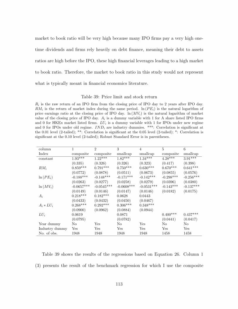
market to book ratio will be very high because many IPO firms pay a very high one-
time dividends and firms rely heavily on debt finance, meaning their debt to assets
ratios are high before the IPO, these high financial leverages leading to a high market
to book ratio. Therefore, the market to book ratio in this study would not represent
what is typically meant in financial economics literature.
Table 39: Price limit and stock return
Ri is the raw return of an IPO firm from the closing price of IPO day to 2 years after IPO day.RMi is the return of market index during the same period. ln (PEi) is the natural logarithm ofprice earnings ratio at the closing price of IPO day. ln (MVi) is the natural logarithm of marketvalue of the closing price of IPO day. Ai is a dummy variable with 1 for A share listed IPO firmsand 0 for HKEx market listed firms. LUi is a dummy variable with 1 for IPOs under new regimeand 0 for IPOs under old regime. INDi are industry dummies. ***: Correlation is significant atthe 0.01 level (2-tailed); **: Correlation is significant at the 0.05 level (2-tailed); *: Correlation issignificant at the 0.10 level (2-tailed); Robust Standard Error is in parentheses.
column 1 2 3 4 5 6Index composite composite smallcap smallcap composite smallcapconstant 1.93*** 1.22*** 1.82*** 1.34*** 4.28*** 3.91***
(0.335) (0.326) (0.326) (0.323) (0.417) (0.398)RMi 0.859*** 0.791*** 0.750*** 0.630*** 0.670*** 0.641***
(0.0772) (0.0878) (0.0511) (0.0673) (0.0855) (0.0576)ln (PEi) -0.188*** -0.148*** -0.171*** -0.142*** -0.298*** -0.256***
(0.0263) (0.0277) (0.0258) (0.0279) (0.0396) (0.0380)ln (MVi) -0.0657*** -0.0545*** -0.0608*** -0.0531*** -0.143*** -0.137***
(0.0149) (0.0146) (0.0147) (0.0146) (0.0182) (0.0175)Ai 0.218*** 0.182*** 0.0628 0.0443
(0.0433) (0.0432) (0.0450) (0.0467)Ai ∗ LUi 0.268*** 0.292*** 0.306*** 0.348***
(0.0900) (0.0962) (0.0884) (0.0944)LUi 0.0619 0.0871 0.400*** 0.437***
(0.0795) (0.0782) (0.0441) (0.0417)Year dummy No Yes No Yes No NoIndustry dummy Yes Yes Yes Yes Yes YesNo. of obs. 1948 1948 1948 1948 1458 1458
Table 39 shows the results of the regressions based on Equation 26. Column 1
(3) presents the result of the benchmark regression for which I use the composite
113

(small capital) index as the market index. Column 2 (4) repeats the regression seen
in Column 1 (3), but I include the year dummy while deleting LUi. The coefficients
of the interaction term Ai ∗ LUi are all positive and significant at a 1% confidence
level for these four specifications. The coefficients of the interaction terms imply that
the 2-year returns of an IPO in the A share market increases by approximately 30%
under the new regime, meaning the price limit has an impact on long-term stock
performance. This percentage is economically significant.
Most of the coefficients of the control variables are also significant. The coefficients
ofRMi are positive and significant at a 1% confidence level for all specifications. These
coefficients are around 0.8, similar to the cross sectional β coefficients. The coefficients
of ln (PEi) are negative and significant at a 1% confidence level. An IPO firm with a
high price earnings ratio will have a poor long-term performance. One possible reason
is that investors are overly optimistic about high PE ratio stocks, and the market
corrects their expectations when the earnings are below their expectation formed on
the IPO day. Coefficients of ln (MVi) are negative and significant at a 1% confidence
level, meaning that small capital stocks have a better long-term performance.
To rule out the impact of the HKEx market’s fluctuation on the results, I run
regressions using only the A share IPOs as a sample. Column 5 (6) of Table 39 presents
the results of the specification, including only the A share IPOs in the sample using
composite (small capital) index as the market index. Though these two specifications
cannot exclude the impact of time trend on long-term stock returns as the difference-
114

in-differences models shown above do, Column 5 and 6 provide the direct change of
long-term stock returns after the consecutive price limit hits at the beginning of the
IPO when the other factors are controlled. The coefficients of LUi indicate that the
2-year stock returns after the IPO increase by approximately 42% in the A share
market under the new policy regime resulting in consecutive price limit hits. These
results are similar to the results given by the difference-in-differences models.
I run the following benchmark regression to investigate the impact of the price
limit policy on the β coefficient.
βi = a0+a1RMi+a2 ln (PEi)+a3 ln (MVi)+a4Ai+a5LUi+a6Ai∗LUi+INDi+ui (27)
where βi is the β coefficient which I calculate using the weekly return from the
IPO day to 2 years after the IPO day. I run an OLS regression with robust standard
errors.
Table 40 shows the results of regressions of Equation 27. Column 1 (3) presents
the results of the benchmark regression in which I use composite (small capital) index
as the market index. Column 2 (4) repeats the regression shown in Column 1 (3),
but I include the year dummy while deleting LUi. The coefficients of the interaction
term Ai ∗ LUi are all positive and significant at a 1% confidence level for these four
specifications. The coefficients of the interaction terms imply that the β coefficient
within 2 years of the IPO in the A share market increases by approximately 0.18
under the new regime during which the price limit has an impact on the long-term
115

Table 40: Price limit and β coefficient
βi is the β coefficient which I calculate using weekly return from IPO day to 2 years after IPO day.RMi is the return of market index during the same period. ln (PEi) is the natural logarithm ofprice earnings ratio at the closing price of IPO day. ln (MVi) is the natural logarithm of marketvalue of the closing price of IPO day. Ai is a dummy variable with 1 for A share listed IPO firmsand 0 for HKEx market listed firms. LUi is a dummy variable with 1 for IPOs under new regimeand 0 for IPOs under old regime. INDi are industry dummies. ***: Correlation is significant atthe 0.01 level (2-tailed); **: Correlation is significant at the 0.05 level (2-tailed); *: Correlation issignificant at the 0.10 level (2-tailed); Robust Standard Error is in parentheses.
column 1 2 3 4 5 6Index composite composite smallcap smallcap composite smallcapconstant 0.483*** 0.358* 1.02*** 0.820*** 2.05*** 2.55***
(0.188) (0.189) (0.178) (0.177) (0.176) (0.155)RMi -0.175*** -0.167*** -0.0949*** -0.110*** -0.194*** -0.0844***
(0.0316) (0.0453) (0.0223) (0.0334) (0.0288) (0.0194)ln (PEi) 0.0429*** 0.0582*** 0.0409*** 0.0623*** 0.000304 0.0107
(0.0163) (0.0179) (0.0152) (0.0170) (0.0149) (0.0128)ln (MVi) 0.0126 0.0156* -0.0129 -0.00800 -0.0429*** -0.0715***
(0.00856) (0.00847) (0.00804) (0.00802) (0.00787) (0.00687)Ai 0.152*** 0.126*** 0.0846*** 0.0565*
(0.0266) (0.0281) (0.0260) (0.0291)Ai ∗ LUi 0.212*** 0.210*** 0.132*** 0.148***
(0.0539) (0.0533) (0.0499) (0.0488)LUi -0.0156 -0.0748 0.215*** 0.0708***
(0.0495) (0.0465) (0.0200) (0.0164)Year dummy No Yes No Yes No NoIndustry dummy Yes Yes Yes Yes Yes YesNo. of obs. 1948 1948 1948 1948 1458 1458
stock performance. This value is economically significant.
Most of the coefficients of the control variables are significant. The coefficients
of RMi are negative and significant at a 1% confidence level for all specifications
at approximately -0.13. The β coefficients of the IPO firms are smaller in the bull
market. The coefficients of ln (PEi) are positive and significant at a 1% confidence
level. An IPO firm with a high price earnings ratio will have a higher β coefficient
because IPO stocks with high PE ratios come with high expectations and are more
116

sensitive to market sentiment and market fluctuation. The coefficients of ln (MV i) are
positive and marginally significant when the composite indices are used to calculate
the β coefficient and negative and insignificant if the small capital indices are used.
This result suggests that there is no apparent relation between the β coefficient and
firm size for IPO firms.
To rule out the impact of the HKEx market’s fluctuation on the results, I run
regressions using only the A share IPOs as a sample. Column 5 (6) of Table 20
presents the result of the specification calculated using the composite (small capital)
index as market index. Though these two specifications cannot eliminate the impact
of time trend on long term β coefficients as the difference-in-differences models shown
above do, Columns 5 and 6 provide the direct change of long-term β coefficient after
consecutive price limit hits at the beginning of the IPO when controlling for other
factors. The coefficients of LUi indicate that the 2-year β coefficients after the IPO
increase by more than 0.14 in the A share market under the new policy regime,
resulting in consecutive price limit hits. These results are similar to those given by
the difference-in-differences models.
I run the following benchmark regression to investigate the impact of the price
limit policy on long-term volatility.
V Li = a0+a1V LMi+a2 ln (PEi)+a3 ln (MVi)+a4Ai+a5LUi+a6Ai∗LUi+INDi+ui
(28)
117

where V Li is the daily average raw volatility of the IPO firm i from the IPO day
until 2 years after, and V LMi is the daily average raw volatility of the market index
from the IPO day of firm i until 2 years after. I run an OLS regression with robust
standard error.
Table 41: Price limit and daily volatility
V Li is the daily average raw volatility of IPO firm i from IPO day to 2 years after IPO day. V LMi
is the daily average raw volatility of the market index from IPO day of firm i to 2 years afterIPO day. ln (PEi) is the natural logarithm of price earnings ratio at the closing price of IPO day.ln (MVi) is the natural logarithm of market value of the closing price of IPO day. Ai is a dummyvariable with 1 for A share listed IPO firms and 0 for HKEx market listed firms. LUi is a dummyvariable with 1 for IPOs under new regime and 0 for IPOs under old regime. INDi are industrydummies. ***: Correlation is significant at the 0.01 level (2-tailed); **: Correlation is significant atthe 0.05 level (2-tailed); *: Correlation is significant at the 0.10 level (2-tailed); Robust StandardError is in parentheses.
column 1 2 3 4 5 6Index composite composite smallcap smallcap composite smallcapconstant 0.0528*** 0.0440*** 0.0512*** 0.0611*** 0.0444*** 0.0442***
(0.00270) (0.00360) (0.00293) (0.00329) (0.00293) (0.00295)V LMi 0.967*** 1.18*** 1.01*** 0.396*** 0.902*** 0.900***
(0.0261) (0.116) (0.0278) (0.0799) (0.0245) (0.0245)ln (PEi) 0.00196*** 0.00240*** 0.00197*** 0.00240*** 0.00116*** 0.00100***
(0.000266) (0.000301) (0.000278) (0.000307) (0.000218) (0.000219)ln (MVi) -0.00188*** -0.00179*** -0.00179*** -0.00176*** -0.00154*** -0.00158***
(0.000128) (0.000128) (0.000138) (0.000131) (0.000134) (0.000134)Ai -0.00498*** -0.00583*** -0.00846*** -0.00547***
(0.000396) (0.000500) (0.000448) (0.000620)Ai ∗ LUi 0.00197** 0.00104 0.00359*** 0.00510***
(0.000933) (0.00103) (0.000944) (0.000954)LUi 0.00455*** 0.00160* 0.00676*** 0.00569***
(0.000891) (0.000903) (0.000233) (0.000242)Year dummy No Yes No Yes No NoIndustry dummy Yes Yes Yes Yes Yes YesNo. of obs. 1948 1948 1948 1948 1458 1458
Table 41 shows the results of the regressions based on Equation 28. Column 1 (3)
presents the result of the benchmark regression using the composite (small capital)
index as the market index. Column 2 (4) repeats the regression shown in Column
118

1 (3) but I include the year dummy while deleting LUi. The coefficients of the
interaction term Ai ∗ LUi are positive and significant at a 5% or higher confidence
level for 3 of the 4 specifications. The coefficients in the regressions using the small
capital index as the market index are more significant than those using the composite
index. Because the IPO firms are mainly small capital firms, the results using small
capital index are more credible. The coefficients of the interaction terms imply that
the daily average volatilities within 2 years of the IPO in the A share market increase
by approximately 0.29% under the new regime after the price limit has an impact on
the long-term stock performance. This increase is economically significant given that
the adjusted average daily volatility is approximately 1% for most of the IPO firms
in the A share market under the old regime.
Most of the coefficients of the control variables are significant. The coefficients of
V LMi are positive and significant at a 1% confidence level for all specifications. The
daily volatilities of the IPO firms are highly affected by the market volatility level.
The coefficients of ln (PEi) are positive and significant at a 1% confidence level. An
IPO firm with a high price earnings ratio will exhibit a higher volatility because IPO
stocks with a high PE ratio come with high expectations and differences in opinions
so that they are more volatile. Coefficients of ln (MVi) are negative and significant at
a 1% confidence level. Because stocks of small capital companies are more volatile,
volatility is highly correlated with firm size, meaning using the small capital index as
the market index to adjust volatility is more appropriate than using the composite
119

index given that most of the IPO firms are small capital firms.
To rule out the impact of the HKEx market’s fluctuation on the results, I run
regressions using only the A share IPOs as a sample. Column 5 (6) of Table 20
presents the result of the specification using the composite (small capital) index as
the market index. Though these two specifications cannot eliminate the impact of
time trend on the long-term average daily volatility as the difference-in-differences
models shown above do, Columns 5 and 6 provide the direct change of the long-term
average daily volatility after consecutive price limit hits at the beginning of the IPO
when other factors are controlled. The coefficients of LUi indicate that the 2-year
average daily volatilities after the IPO increase by more than 0.62% in the A share
market under the new policy regime, resulting in consecutive price limit hits. These
results are consistent with those given by the difference-in-differences models.
I run the following benchmark regression to investigate the impact of the price
limit policy on the long-term liquidity.
TOi = a0+a1TOMi+a2 ln (PEi)+a3 ln (MVi)+a4Ai+a5LUi+a6Ai∗LUi+INDi+ui
(29)
where TOi is the daily average raw turnover of the IPO firm i from the IPO day to
2 years after, and TOMi is the daily average raw turnover of the market index from
the IPO day of firm i to 2 years after. I run an OLS regression with robust standard
errors.
120

Table 42: Price limit and daily turnover
TOi is the daily average raw turnover of IPO firm i from IPO day to 2 years after IPO day. TOMi
is the daily average raw turnover of the market index from IPO day of firm i to 2 years afterIPO day. ln (PEi) is the natural logarithm of price earnings ratio at the closing price of IPO day.ln (MVi) is the natural logarithm of market value of the closing price of IPO day. Ai is a dummyvariable with 1 for A share listed IPO firms and 0 for HKEx market listed firms. LUi is a dummyvariable with 1 for IPOs under new regime and 0 for IPOs under old regime. INDi are industrydummies. ***: Correlation is significant at the 0.01 level (2-tailed); **: Correlation is significant atthe 0.05 level (2-tailed); *: Correlation is significant at the 0.10 level (2-tailed); Robust StandardError is in parentheses.
column 1 2 3Index composite composite compositeconstant 0.128*** 0.111*** 0.289***
(0.00827) (0.00836) (0.0141)TOMi 0.0507 -0.327*** 0.0677
(0.0713) (0.102) (0.0768)ln (PEi) 0.000820 0.00289*** -0.000139
(0.000550) (0.000601) (0.00103)ln (MVi) -0.00555*** -0.00506*** -0.0106***
(0.000385) (0.000377) (0.000632)Ai 0.0447*** 0.0470***
(0.00111) (0.00142)Ai ∗ LUi 0.0331*** 0.0320***
(0.00151) (0.00183)LUi -0.00397*** 0.0302***
(0.000871) (0.00123)Year dummy No Yes NoIndustry dummy Yes Yes YesNo. of obs. 1948 1948 1458
Table 42 shows the results of the regressions based on Equation 29. Column 1
presents the result of the benchmark regression when I use the composite index as
the market index. Column 2 repeats the regression shown in Column 1, but I include
the year dummy while deleting LUi. The coefficients of the interaction term Ai ∗LUi
are positive and significant at a 1% confidence level for both specifications. The
coefficients of the interaction terms in Columns 1 and 2 imply that the daily average
turnovers within 2 years of the IPO in the A share market increase by approximately
121

3.3% under the new regime, meaning price limit has an impact on long-term stock
performance. This increase is economically significant given that the adjusted average
daily turnover is approximately 3.5% for most of the IPO firms in the A share market
under the old regime.
Most of the coefficients of the control variables are significant. The coefficients of
TOMi are positive in Column 1 but negative in Column 2. IPO firms’ turnovers are
not as sensitive to the market as the volatilities and stock returns. The coefficients
of ln (PEi) are positive and significant at a 1% confidence level. An IPO firm with
a high price earnings ratio will have a high turnover because IPO stocks with a high
PE ratio come with high expectations and differences in opinions, meaning they are
held by investors for a shorter period. The coefficients of ln (MVi) are negative and
significant at a 1% confidence level, again showning stocks of small capital companies
are held by investors for a shorter period.
To rule out the impact of the HKEx market’s fluctuation on the results, I run re-
gressions using only the A share IPOs as a sample. Column 3 of Table 20 presents the
result of the specification when using composite index as the market index. Though
this specification cannot eliminate the impact of time trend on the long-term aver-
age daily turnover as the difference-in-differences models shown above do, Column 3
provides the direct change of the long-term average daily turnovers after consecutive
price limit hits at the beginning of the IPO when other factors are controlled. The
coefficients of LUi indicate that the 2-year average daily turnovers after the IPO in-
122

crease by more than 3.0% in the A share market under the new policy regime resulting
in consecutive price limit hits. These results are consistent with those given by the
difference in differences models.
2.5 Summary and Conclusions
In this paper, I explored the impact of the price limit policy on long-term stock
performance. Using IPOs on the Chinese A share market and the HKEx market from
2006 to 2015, I employed a difference-in-differences method to investigate whether a
new IPO policy for the A share market causing consecutive limit-ups at the beginning
period of the IPO has long-term effects on stock returns, turnovers, volatility and β
coefficients. I obtained the following results.
First, the 2-year stock returns after the IPO increase by approximately 30% in the
A share market under the new policy regime causing the consecutive limit-up hits.
The median of the adjusted 2-year stock returns under the old regime was -9.59% (-
14.98%) if the composite (small capital) index is used to adjust for raw returns. This
increase in stock returns caused by the price limit rule is significant economically.
Moreover, the 2-year β coefficients after the IPO increase by approximately 0.18
in the A share market under the new policy regime. This increase is almost the
standard deviation of the β coefficients of the IPO firms under the old regime.
In addition, the 2-year daily average volatilities after the IPO increase by approx-
imately 0.29% in the A share market under the new policy regime. The median of the
raw daily average volatilities under the old regime was 2.79%, meaning the increase in
123

volatilities caused by the price limit rule is approximately 10% of the original volatili-
ties. However, the results are more significant when considering only the results using
the small capital index as the market index.
Finally, the 2-year daily average turnovers after the IPO increase by approximately
3.2% in the A share market under the new policy regime. The median of the raw daily
average turnovers under the old regime was 4.56%, meaning the increase in turnovers
caused by the price limit rule is approximately 70% of the original turnovers. This
increase in turnovers caused by price limit rule is also significant economically.
The empirical results are consistent with the hypothesis that the price limit policy
results in the IPO firms in the A share market having larger stock returns, turnovers,
volatility and β coefficients over a 2-year period after the IPO. A possible explanation
for these results is that the consecutive limit up hits at the beginning of an IPO attract
investors with a high risk preference. This impact on the investor structure of an IPO
firm has long-term effects on its stock performance including stock return, turnover,
volatility and β coefficient.
As with all research, this study has limitations. Although the empirical results
support the hypotheses in this paper, I cannot rule out other factors. For example,
if the change in such variables as stock return and turnover in the Chinese stock
market compared with the Hong Kong stock market began before the enactment of
the IPO policy in the former, it is likely that other factors caused this change. A
potential reason is that the new IPO policy restricted the amount of capital raised
124

in the IPO, so firms have an incentive to increase earnings to make seasoned equity
offerings at higher price after they are listed. As the difference-in-differences methord
used here cannot rull out these other factors, it can only provide evidence that the
hypothesis raised in this paper is supported by the empirical results, and these results
are consistent with the hypotheses.
3 Do Investors Invest in Familiarity? Evidence
from the Shanghai-Hong Kong Stock Connect
3.1 Introduction
There are two stock exchanges in the mainland China, one in Shanghai, the other
in Shenzhen, and only one in Hong Kong. Before the mainland Hong Kong stock
connect policy, it was difficult for investors in Hong Kong to trade stocks listed on
the mainland China stock exchanges, and vice versa. In 2014, the Hong Kong and the
Shanghai Stock Exchanges launched the Shanghai-Hong Kong Stock Connect, with
the Shenzhen-Hong Kong Stock Connect being introduced two years later. These
Stock connect policies allow investors at one location to conveniently buy stocks
listed at the other.
In this paper, I test the effect of the Shanghai-Hong Kong Stock Connect on the
Chinese stock market. More specifically, I investigate whether investors in Hong Kong
who began to invest in the Shanghai stock market was more likely to buy companies
which were also dual-listed on the Hong Kong Stock Exchange and whether this effect
weakened gradually as they became familiar with the companies listed only on the
125

Shanghai stock market.
When stocks become constituents of indices, they become thetarget of passive
management funds, meaning their investor base enlarges, the impact of this member-
ship being documented by scholars. For example, Morck and Yang (2001) found a
large value premium in the average q ratios of firms in the S&P 500 index relative
to the q ratios of similar firms. They documented that passive investment strategies
requiring the purchase of the specific 500 stocks in this index increase demand for
them, pushing up their prices. In their investigation of the effect of this change on the
price, Chen, Noronha and Singal (2004) found that there is a permanent increase in
the price of the new firms but no permanent decline in the deleted ones. This asym-
metric price effect of the S&P 500 index additions and deletions can be attributed to
changes in investor awareness.
In future research, Robinson, Kleffner and Bertels (2011) documented that being
added to the Dow Jones Sustainability World Index (DJSI) results in a sustained
increase in a firm’s share price, but there is a temporary decrease in value for the first
10 days after being removed. Using a sample of S&P 500 additions between 1976-
2001, Cai (2007) found a significantly positive price reaction but no volume reaction
for the industry- and size-matched firms, with the matching-firm price reaction being
negatively related to the added firms’s weight in its industry.
Some literature documents that investors are more likely to invest in local firms.
For example, Huberman (2001) documented that household portfolios tend to be
126

concentrated, that employees tend to own their employers’ stocks in their retirement
account, and as have others, found a home country bias in the international arena.
As these phenomena suggest, people invest in familiarity, a conclusion suggested by
Ivkovic and Weisbenner (2005) who documented that households exhibit a strong
preference for local investments. They found that the average household generates an
additional annualized return of 3.2% from its local holdings relative to its nonlocal
holdings, and excess returns from investing locally are even larger among stocks not
in the S&P 500 index. They are receiving higher returns due to this preference.
In early research, Coval and Moskowits (1999) found that U.S. investment man-
agers exhibit a strong preference for locally headquartered firms, particularly small,
highly levered firms that produce nontraded goods, results consistent with the hy-
pothesis that asymmetric information between local and nonlocal investors drive the
preference for geographically proximate investments. Strong and Xu (2003) used
survey data from fund managers on the prospects for international equity markets
to investigate why investment portfolios are significantly biased towards domestic
equities, finding that fund managers from the United States, the United Kingdom,
continental Europe, and Japan show a significant relative optimism towards their
home equity markets.
Other research investigates the impact of opening stock markets to foreign in-
vestors, including an examination of their investment behavior. For example, Kim
and Singal’s (2000) examination of the effects associated with the opening of a stock
127

market found that stock returns increase immediately after the opening without a
concomitant increase in volatility and that stock markets function more efficiently.
Using data on foreign stock ownership in Japan from 1975 to 1991, Kang and Stulz
(1997) showed that foreign investors overweight shares of firms in the manufacturing
sector, large firms, and firms with good accounting performance, with low unsystem-
atic risk, and with low leverage, and that small firms with a high level of exports have
greater foreign ownership controlling for size.
Using data from 2014 to 2016 from the Chinese stock market, I find in this paper
that stocks dual-listed on the Shanghai and Hong Kong stock markets have higher
monthly stock returns than those on the Shanghai-Hong Kong stock connect but
listed only in Shanghai; however, this difference in stock returns decreases gradually.
Moreover, stocks dual-listed in Shanghai and Hong Kong have a higher daily average
turnover than stocks on the Shanghai-Hong Kong stock connect but listed only in
Shanghai; however, this difference also decreases gradually. These empirical results
are consistent with the hypothesis expolored in this paper that Hong Kong investors
were more likely to buy Shanghai-Hong Kong dual-listed stocks through the stock
connect channel in the beginning and that they extended their investment target to
stocks involved in the stock connect but listed only in Shanghai after they gained
experience and became familiar with Shanghai stock market. Section 2 presents the
hypotheses, while Section 3 provides the descriptive statistics of the data and the
variables, and Section 4 shows the empirical results. Section 5 provides implications
128

and limitations.
3.2 the Hypotheses
Two kinds of stocks are included in the Hong Kong mainland stock connect policy,
those listed on both the Hong Kong Stock Exchange and the Shanghai Stock Exchange
(or Shenzhen for Shenzhen-Hong Kong stock connect) already, and other blue chips
listed only on a single exchange and are constituent stocks of the market indices. For
the Shanghai-Hong Kong Stock Connect, the Shanghai stocks involved are constituent
stocks of the SSE 180 Index and the SSE 380 Index; while the Hong Kong stocks are
constituent stocks of the Hang Seng Composite LargeCap Index and the Hang Seng
Composite MidCap Index. For Shenzhen-Hong Kong Stock Connect, the Shenzhen
stocks are constituent stocks of the Shenzhen Component Index and the Shenzhen
SME Innovation Index with a market value of more than 6 billion Chinese yuan; while
the Hong Kong stocks are those on the Shanghai-Hong Kong stock connect and the
constituent stocks of the Hang Seng Composite SmallCap Index with a market value
of more than 5 billion Hong Kong Dollar.
At the beginning of the enactment of Shanghai Hong Kong stock connect polity,
the Hong Kong investors were not familiar with the stocks not listed on their stock
exchange, meaning they were more likely to buy Shanghai-Hong Kong dual-listed
stocks through the stock connect channel. However, after they gained experience
and became familiar with the Shanghai stock market, they extended their investment
target to stocks involved in the stock connect but listed only in Shanghai. Hence,
129

the Shanghai-Hong Kong dual-listed stocks exhibited better performance and larger
transaction volumes than those on the Shanghai-Hong Kong stock connect immedi-
ately after it was enacted, however, the differences in stock returns and transaction
volumes gradually decreased. Therefore, I hypothesize:
H1a: Stocks dual-listed in Shanghai and Hong Kong have higher monthly stock
return than stocks on the Shanghai-Hong Kong stock connect but listed only in
Shanghai.
H1b: The difference in stock returns between the dual-listed and other stocks on
the Shanghai-Hong Kong stock connect decreases gradually.
H2a: Stocks dual-listed in Shanghai and Hong Kong have higher daily average
turnovers than stocks on the Shanghai-Hong Kong stock connect but listed only in
Shanghai.
H2b: The difference in the daily average turnovers between dual-listed and other
stocks on the Shanghai-Hong Kong stock connect decreases gradually.
3.3 The Data and Variables
The Shanghai Hong Kong stock connect opened on November 17, 2014, while the
Shenzhen Hong Kong stock connect was launched approximately two years later in
December 5, 2016. Data between these two dates are used as the sample here for
conducting a difference-in-differences test. Monthly data are used in this research,
with 35087 observations being used in this 25-month period. These data come from
the WIND Database, which is a major producer of data on the Chinese financial
130

market. During this sample period, stocks listed in Shanghai but which are also
involved in the Shanghai Hong Kong stock connect were affected by the policy, while
stocks listed in Shenzhen were not, meaning four kinds of stocks are included in
this research: stocks listed in both Shanghai and Hong Kong, stocks listed only in
Shanghai and involved in Shanghai Hong Kong stock connect, stocks listed in both
Shenzhen and Hong Kong, and stocks listed only in Shenzhen and are constituent
stocks of Shenzhen Component Index and Shenzhen SME Innovation Index. The last
kind of stocks are expected to be involved in Shenzhen Hong Kong stock connect when
it is launched. The latter two kinds are used as control groups to address influence
from other factors. The variables used in this paper are as follows:
• SHHit is a dummy variable with 1 representing firms listed in Shanghai and 0
for firms listed in Shenzhen;
• HKit is a dummy variable with 1 representing firms dual-listed in Hong Kong
and Shanghai (or Shenzhen) and 0 for firms listed in only Shanghai (or Shen-
zhen);
• TVit is the market value of tradable shares of Firm i at the end of quarter t,
tvit = ln (TVit);
• Rit is the return for Stock i in Month t;
• V Lit is the daily average volatility for Firm i in Month t, a volatility derived
from the standard deviation of daily stock returns over a month;
131

• TOit is the daily average turnover rate for Firm i in Month t, defined as the
ratio of the transaction volume to tradable shares;
• CLit is the closing price of Firm i at the end of Month t, clit = ln (CLit);
• βit is the β coefficient of Firm i at the end of Month t calculated using monthly
returns for the prior 24 months;
• BMit is the book to market ratio at the end of period t; if the book value is
negative, then I assign a very small value for the book to market ratio to this
firm which will subsequently be winsorized; bmit = ln (BMit);
• ROEit is the return on equity of Firm i for the most recent four consecutive
quarters before Month t; I use earnings before abnormal terms as the numerator
and the book equity at the end of the period as the denominator to calculate
the return on equity;
• AGit is the year over year percentage growth of total assets for Firm i at the
end of the most recent quarter before Month t, agit = ln (1 + AGit).
The definition of the recent quarter is as follows. For bmit, ROEit, agit, I use
financial data available to investors at the beginning of Month t if I use the return
of this month as the subsequent return. For example, if I use data from March 2017
to calculate the subsequent return, I will use the financial data in the third quarter
report of 2016 to calculate bmit, ROEit, agit because listed companies are required
132

to release their annual reports for 2016 and the first quarter report for 2017 no later
than April 30, 2017.
To avoid the impact of extreme values on the results, I winsorize all variables
in this paper. For agit,βit, ROEit, Rit, I replace observations within the bottom
or top 0.01 quantiles of the variables by the bottom or top 0.01 quantile values of
the variables, respectively. For bmit, I replace observations within the bottom 0.02
quantile of the variable by the bottom 0.02 quantile value of the variable. For tvit, clit,
TOit, V Lit, I replace observations within the top 0.02 quantiles of the variables by
the top 0.02 quantile values of the variables, respectively. I winsorize some variables
on only one side because extreme values are unlikely to appear on the other.
Table 43 presents the descriptive statistics as raw data before winsorizing. SH AH
refers to firms dual-listed on both the Shanghai Stock Exchange and the Hong Kong
Stock Exchange; SH A refers to firms listed only on the Shanghai Stock Exchange
but also involved in the Shanghai Hong Kong stock connect; SZ AH refers to firms
dual-listed on the Shenzhen Stock Exchange and the Hong Kong Stock Exchange; SZ
A refers to firms listed on the Shenzhen Stock Exchange and are constituent stocks
of the Shenzhen Component Index and Shenzhen SME Innovation Index.
Because the data are not winsorized, medians are more representative than means.
The medians of the market value of tradable shares indicate that dual-listed firms are
larger than firms listed only in mainland China, and firms listed on the Shanghai
Stock Exchange are larger than those listed on the Shenzhen Stock Exchange. The
133
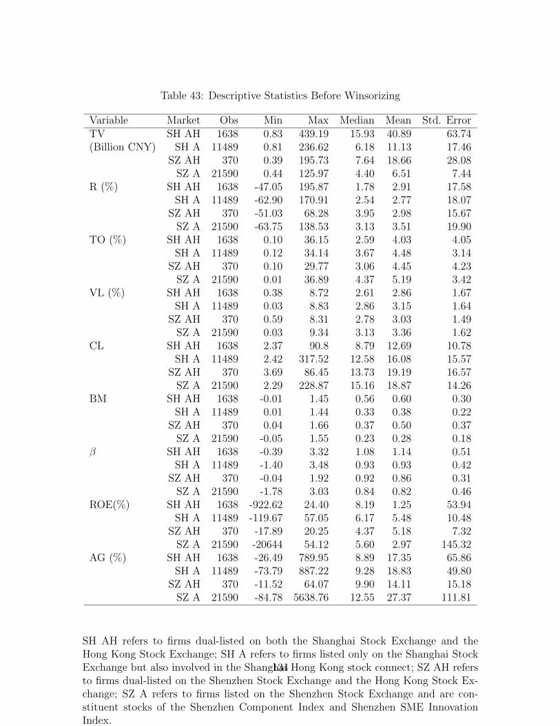
Table 43: Descriptive Statistics Before Winsorizing
Variable Market Obs Min Max Median Mean Std. ErrorTV SH AH 1638 0.83 439.19 15.93 40.89 63.74(Billion CNY) SH A 11489 0.81 236.62 6.18 11.13 17.46
SZ AH 370 0.39 195.73 7.64 18.66 28.08SZ A 21590 0.44 125.97 4.40 6.51 7.44
R (%) SH AH 1638 -47.05 195.87 1.78 2.91 17.58SH A 11489 -62.90 170.91 2.54 2.77 18.07
SZ AH 370 -51.03 68.28 3.95 2.98 15.67SZ A 21590 -63.75 138.53 3.13 3.51 19.90
TO (%) SH AH 1638 0.10 36.15 2.59 4.03 4.05SH A 11489 0.12 34.14 3.67 4.48 3.14
SZ AH 370 0.10 29.77 3.06 4.45 4.23SZ A 21590 0.01 36.89 4.37 5.19 3.42
VL (%) SH AH 1638 0.38 8.72 2.61 2.86 1.67SH A 11489 0.03 8.83 2.86 3.15 1.64
SZ AH 370 0.59 8.31 2.78 3.03 1.49SZ A 21590 0.03 9.34 3.13 3.36 1.62
CL SH AH 1638 2.37 90.8 8.79 12.69 10.78SH A 11489 2.42 317.52 12.58 16.08 15.57
SZ AH 370 3.69 86.45 13.73 19.19 16.57SZ A 21590 2.29 228.87 15.16 18.87 14.26
BM SH AH 1638 -0.01 1.45 0.56 0.60 0.30SH A 11489 0.01 1.44 0.33 0.38 0.22
SZ AH 370 0.04 1.66 0.37 0.50 0.37SZ A 21590 -0.05 1.55 0.23 0.28 0.18
β SH AH 1638 -0.39 3.32 1.08 1.14 0.51SH A 11489 -1.40 3.48 0.93 0.93 0.42
SZ AH 370 -0.04 1.92 0.92 0.86 0.31SZ A 21590 -1.78 3.03 0.84 0.82 0.46
ROE(%) SH AH 1638 -922.62 24.40 8.19 1.25 53.94SH A 11489 -119.67 57.05 6.17 5.48 10.48
SZ AH 370 -17.89 20.25 4.37 5.18 7.32SZ A 21590 -20644 54.12 5.60 2.97 145.32
AG (%) SH AH 1638 -26.49 789.95 8.89 17.35 65.86SH A 11489 -73.79 887.22 9.28 18.83 49.80
SZ AH 370 -11.52 64.07 9.90 14.11 15.18SZ A 21590 -84.78 5638.76 12.55 27.37 111.81
SH AH refers to firms dual-listed on both the Shanghai Stock Exchange and theHong Kong Stock Exchange; SH A refers to firms listed only on the Shanghai StockExchange but also involved in the Shanghai Hong Kong stock connect; SZ AH refersto firms dual-listed on the Shenzhen Stock Exchange and the Hong Kong Stock Ex-change; SZ A refers to firms listed on the Shenzhen Stock Exchange and are con-stituent stocks of the Shenzhen Component Index and Shenzhen SME InnovationIndex.
134

medians of returns are slightly lower for the dual-listed firms in Shanghai while this
result is opposite for the dual-listed firms in Shenzhen. The medians of both daily
average turnover and daily average volatility are lower for dual-listed firms than for
the other stocks on both the Shanghai and Shenzhen stock exchanges. The medians
of both the book-market ratios and the beta coefficients are lower for the dual-listed
firms than for the other stocks on both the Shanghai and Shenzhen stock exchanges.
The medians of the returns on equity are higher for the dual-listed firms in Shanghai
while the result is opposite for the dual-listed firms in Shenzhen. The medians of the
growth rate of total assets are lower for the dual-listed firms than for the other firms.
Table 44 presents the descriptive statistics after winsorizing, meaning the means
of the variables are not affected by extreme values. The means of the market values of
tradable shares indicate that the dual-listed firms have a larger size than firms listed
only in mainland China, and firms listed on the Shanghai Stock Exchange are larger
than those listed on the Shenzhen Stock Exchange. All four kinds stocks have similar
monthly returns, though the means of returns are slightly lower for the dual-listed
firms on both the Shanghai and Shenzhen stock exchanges. The means of both the
daily average turnovers and the daily average volatility are lower for the dual-listed
firms than for the other stocks for both the Shanghai and Shenzhen stock exchanges.
The means of both the book-market ratios and the beta coefficients are lower for the
dual-listed firms than for the other stocks for both the Shanghai and Shenzhen stock
exchanges. The returns on equity are similar for all four types of firms, while means
135

Table 44: Descriptive Statistics After Winsorizing
Variable Market Obs Min Max Median Mean Std. ErrorTV SH AH 1638 0.83 55.13 15.93 23.53 19.27(Billion CNY) SH A 11489 0.81 55.13 6.18 10.15 10.99
SZ AH 370 0.39 55.13 7.64 15.19 14.59SZ A 21590 0.44 55.13 4.40 6.42 6.64
R (%) SH AH 1638 -45.45 56.36 1.78 2.59 15.78SH A 11489 -45.45 56.36 2.54 2.66 17.44
SZ AH 370 -45.45 56.36 3.95 2.97 15.47SZ A 21590 -45.45 56.36 3.13 3.40 19.14
TO (%) SH AH 1638 0.10 13.98 2.59 3.91 3.57SH A 11489 0.12 13.98 3.67 4.44 2.98
SZ AH 370 0.10 13.98 3.06 4.22 3.26SZ A 21590 0.01 13.98 4.37 5.11 3.13
VL (%) SH AH 1638 0.38 7.56 2.61 2.85 1.64SH A 11489 0.03 7.56 2.86 3.14 1.61
SZ AH 370 0.59 7.56 2.78 3.03 1.48SZ A 21590 0.03 7.56 3.13 3.35 1.60
CL SH AH 1638 2.37 56.40 8.79 12.57 10.15SH A 11489 2.42 56.40 12.58 15.49 10.43
SZ AH 370 3.69 56.40 13.73 18.76 15.36SZ A 21590 2.29 56.40 15.16 18.32 11.59
BM SH AH 1638 0.06 1.45 0.56 0.60 0.30SH A 11489 0.06 1.44 0.33 0.38 0.22
SZ AH 370 0.06 1.66 0.37 0.51 0.37SZ A 21590 0.06 1.55 0.23 0.28 0.18
β SH AH 1638 -0.28 2.09 1.08 1.13 0.46SH A 11489 -0.28 2.09 0.93 0.93 0.40
SZ AH 370 -0.04 1.92 0.92 0.86 0.31SZ A 21590 -0.28 2.09 0.84 0.82 0.45
ROE(%) SH AH 1638 -37.33 24.40 8.19 5.50 12.39SH A 11489 -37.33 26.89 6.17 5.62 8.99
SZ AH 370 -17.89 20.25 4.37 5.18 7.32SZ A 21590 -37.33 26.89 5.60 5.11 9.43
AG (%) SH AH 1638 -21.71 220.62 8.89 13.61 28.88SH A 11489 -21.71 220.62 9.28 17.12 32.32
SZ AH 370 -11.52 64.07 9.90 14.11 15.18SZ A 21590 -21.71 220.62 12.55 23.32 37.83
SH AH refers to firms dual-listed on both the Shanghai Stock Exchange and theHong Kong Stock Exchange; SH A refers to firms listed only on the Shanghai StockExchange but also involved in the Shanghai Hong Kong stock connect; SZ AH refersto firms dual-listed on the Shenzhen Stock Exchange and the Hong Kong Stock Ex-change; SZ A refers to firms listed on the Shenzhen Stock Exchange and are con-stituent stocks of the Shenzhen Component Index and Shenzhen SME InnovationIndex.
136

of the growth rate of total assets are lower for the dual-listed firms than other firms.
3.4 Empirical Results
I use a difference-in-differences method to test the hypothesis whether investors in
Hong Kong view Shanghai Hong Kong dual-listed stocks and other Shanghai Hong
Kong stock connect involved stocks differently. I run the following Fama-MacBeth
cross-sectional regression for each month during the sample peried.
Rit+1 = a0 + a1shhit + a2hkit + a3shhit ∗ hkit + a4Rit + a5clit + a6βit
+a7bmit + a8V Lit + a9TOit + a10tvit + a11ROEit + a12agit + eit
(30)
Column 1 of Table 45 shows the estimate results of Equation 1.
The coefficient of the interaction term hkit ∗ shhit is positive though insignificant,
suggesting that the monthly return of a dual-listed firm is 1.1% higher than that of a
firm listed only in Shanghai and involved in the Shanghai Hong Kong stock connect,
controlling for other variables which affect stock returns. This difference is econom-
ically significant at 14.03% annually, a result that is consistent with Hypothesis 1a.
Because investors in Hong Kong are not familiar with the firms listed only on the
Shanghai stock exchange, they prefer to buy those dual-listed on the Shanghai and
Hong Kong stock exchanges than firms listed only on Shanghai stock exchange when
they buy stocks through the Shanghai Hong Kong stock connect. The coefficients
of Rit, TOit and tvit are all negative and significant, indicating that higher current
stock returns, turnovers, and firm size predict lower stock returns in the subsequent
137

Table 45: Impact of Shanghai Hong Kong Stock Connect on Stock Returns andTurnovers
SHHit is a dummy variable with 1 for firm listed in Shanghai and 0 for firms listed in Shenzhen;HKit is a dummy variable with 1 for firm dual-listed in Hong Kong and Shanghai (or Shenzhen)and 0 for firms listed in only Shanghai (or Shenzhen);CLit is the closing price of firm i at the endof period t; clit = ln (CLit); Rit is the return for stock i in month t; TVit is the market value oftradable shares of firm i at the end of period t; tvit = ln (TVit); ROEit is return on equity of firm iin the recent four consecutive quarters before month t; AGit is year over year percentage growth oftotal asset for firm i at the end of the most recent quarter before month t;agit = ln (1 +AGit); BMit
is the book to market equity ratio at the end of period t;bmit = ln (BMit); βit is the β coefficientof firm i at the end of month t; V Lit is the daily average volatility for firm i in month t; TOit isthe daily average turnover rate for firm i in month t; ***: Coefficient is significant at the 0.01 level(2-tailed); **: Coefficient is significant at the 0.05 level (2-tailed); *: Coefficient is significant at the0.10 level (2-tailed); Standard errors adjusted for autocorrelation are in parentheses.
Column 1 2Dependent Rit+1 TOit+1
constant 0.276** 0.080***(0.104) (0.011)
hkit -0.001 0.000(0.007) (0.001)
shhit -0.007* -0.001***(0.003) (0.000)
hkit ∗ shhit 0.011 0.001(0.008) (0.002)
Rit -0.066** 0.009(0.031) (0.008)
clit -0.005 0.000(0.006) (0.001)
βit -0.002 0.002**(0.003) (0.001)
bmit 0.002 -0.001***(0.005) (0.000)
V Lit 0.201 -0.182***(0.202) (0.041)
TOit -0.340*** 0.693***(0.098) (0.025)
tvit -0.011** -0.003***(0.004) (0.000)
ROEit 0.008 -0.012***(0.017) (0.001)
agit 0.003 0.002**(0.005) (0.001)
138

month.
Column 8 in Table 46 and Figure 18 show the coefficients of the interaction terms
in Equation 1 for each month, all of which are above 0.05 for the first two months
after the enactment of the Shanghai Hong Kong stock connect. These are significant
at 1% in the second month before following a descending trend afterward, a trend
consistent with hypothesis 1b. The difference in stock return between firms dual-listed
in Shanghai and Hong Kong and firms listed only in the Shanghai but involved in
Shanghai Hong Kong stock connect decreases gradually. As investors in Hong Kong
gain familiarity with firms listed only in Shanghai, they began to treat them the same
as the dual-listed firms.
To test Hypothesis 2a, I run the following Fama-MacBeth cross-sectional regres-
sion for each month during the sample period.
TOit+1 = a0 + a1shhit + a2hkit + a3shhit ∗ hkit + a4Rit + a5clit + a6βit
+a7bmit + a8V Lit + a9TOit + a10tvit + a11ROEit + a12agit + eit
(31)
Column 2 of Table 45 shows the estimate results of Equation 2. The coefficient
of the interaction term hkit ∗ shhit is positive though insignificant, implying that the
daily average turnovers in the subsequent month of a dual-listed firm is 0.1% higher
than that of a firm listed only in Shanghai and involved in the Shanghai Hong Kong
stock connect, controlling for other variables which affect turnovers. This difference
is approximately 3% of the daily average turnover of a Shanghai Hong Kong dual-
listed stock, which is economically significant considering that transactions through
139

the Shanghai Hong Kong stock connect are approximately 0.5% of the total daily
transactions on the Chinese stock market, a result consistent with hypothesis 2a.
Investors in Hong Kong prefer to buy firms dual-listed on the Shanghai and Hong
Kong stock exchanges than firms listed only on the Shanghai stock exchange when
they buy stocks through Shanghai Hong Kong stock connect. The coefficients of βit,
TOit and agit are all positive and significant, while the coefficients of bmit, V Lit, tvit
and ROEit are all negative and significant, indicating that the higher beta coefficients,
turnovers, growth rates of total assets predict lower subsequent daily turnovers while
higher book-market ratios, volatility, firm sizes and returns on equity predict lower
daily turnovers in the subsequent month.
Column 8 in Table 48 and Figure 20 present the coefficients of the interaction
terms in Equation 2 for each month. These coefficients which are above 0.008 for the
first two months after the enactment of the Shanghai-Hong Kong stock connect, are
significant at 1% in the second month followed by a subsequent descending trend.
This trend is consistent with Hypothesis 2b. The gap in the subsequent daily average
turnover between firms dual-listed in Shanghai and Hong Kong and firms listed only in
Shanghai but involved in the Shanghai-Hong Kong stock connect decreases gradually.
As investors in Hong Kong gain familiarity with the firms listed only in Shanghai,
they began to trade them similar to trading dual-listed firms.
Table 46 presents the stock returns for each month after the enactment of the
Shanghai-Hong Kong stock connect. Columns 1 and 2 show the raw monthly re-
140

turns of firms dual-listed on the Shanghai Stock Exchange and the Hong Kong Stock
Exchange, and the raw monthly returns of firms listed only on the Shanghai Stock
Exchange but involved in the Shanghai-Hong Kong stock connect. Column 3 shows
the difference between the returns of these two types of firms, while Columns 4 and
5 present the raw monthly returns of firms dual-listed on the Shenzhen Stock Ex-
change and the Hong Kong Stock Exchange and the raw monthly returns of firms
listed only on the Shenzhen Stock Exchange and are constituent stocks of Shenzhen
Component Index and Shenzhen SME Innovation Index, respectively. Column 6
shows the difference between the returns of these two types of firms, and Column 7
shows the difference between the return differences in Columns 3 and 6, which is the
difference-in-differences of the stock returns between the dual-listed and the Shang-
hai (Shenzhen) Stock Exchange listed firms between the Shanghai Stock Exchange
(already affected by the Shanghai-Hong Kong stock connect) and the Shenzhen Stock
Exchange (not yet affected by the Shenzhen-Hong Kong Stock connect). The standard
errors are shown in parentheses. Column 7 and Figure 18 show that the difference-in-
differences returns are positive for 17 of the 25 months. These difference-in-differences
returns are above 7% per month and statistically significantly different from zero in
the first two months, and these difference-in-differences returns began to decrease
gradually afterwards, a trend consistent with Hypothesis 1b. The gap in subsequent
returns between the firms dual-listed in Shanghai and Hong Kong and the firms listed
only in Shanghai but involved in the Shanghai-Hong Kong stock connect decreases
141

gradually.
Table 46: Mean of monthly returns after enactment of Shanghai Hong Kong StockConnect
Month A HKEx DIF-IN-DIFColumn 1 2 3 4 5 6 7 8Stocks SH AH SH A DIF SZ AH SZ A DIF DID Coef.1 26.76 16.05 10.71 14.62 11.23 3.39 7.32*(4.04) 0.054(0.037)2 11.70 -0.96 12.66 0.92 -4.09 5.01 7.65***(2.78) 0.074***(0.026)3 -6.51 4.68 -11.19 1.51 10.19 -8.68 -2.51(3.40) -0.013(0.031)4 9.18 11.54 -2.36 6.47 12.54 -6.07 3.71(2.71) 0.032(0.026)5 23.51 20.32 3.19 21.84 21.57 0.27 2.92(4.14) 0.031(0.040)6 4.07 8.00 -3.93 5.59 13.06 -7.47 3.54(4.55) 0.031(0.042)7 15.66 25.21 -9.55 19.19 26.53 -7.34 -2.21(4.78) -0.009(0.041)8 -21.50 -34.09 12.59 -28.53 -35.49 6.96 5.63(3.45) 0.072**(0.030)9 9.36 19.37 -10.01 14.70 19.18 -4.48 -5.53(4.65) -0.018(0.040)10 -20.97 -28.03 7.06 -25.11 -31.94 6.83 0.23(3.22) 0.023(0.030)11 9.36 17.17 -7.81 13.08 24.92 -11.84 4.03(4.04) 0.029(0.031)12 5.03 9.35 -4.32 7.20 15.94 -8.74 4.42(3.67) 0.043(0.035)13 -4.18 -1.70 -2.48 2.19 1.51 0.68 -3.16(3.31) -0.017(0.032)14 -16.37 -21.32 4.95 -14.65 -23.85 9.2 -4.25(3.07) -0.033(0.028)15 -0.98 0.05 -1.03 -0.36 2.77 -3.13 2.10(2.99) 0.032(0.027)16 2.12 -2.75 4.87 -1.30 -5.74 4.44 0.43(2.69) 0.018(0.024)17 6.41 14.25 -7.84 11.10 19.26 -8.16 0.32(3.02) 0.009(0.027)18 -7.58 -8.94 1.36 -8.23 -9.34 1.11 0.25(2.99) 0.024(0.028)19 -0.09 1.95 -2.04 -1.10 4.88 -5.98 3.94(3.09) 0.040(0.030)20 8.71 9.37 -0.66 10.23 9.09 1.14 -1.80(2.51) -0.005(0.024)21 1.73 2.07 -0.34 14.85 -0.65 15.5 -15.84***(2.28) -0.147***(0.021)22 -3.67 -2.91 -0.76 -8.13 -2.03 -6.1 5.34**(2.14) 0.0493(0.0207)23 2.80 3.28 -0.48 8.16 3.82 4.34 -4.82***(1.62) -0.049***(0.016)24 6.46 4.24 2.22 4.68 3.77 0.91 1.31(2.25) 0.003(0.021)25 1.78 -1.35 3.13 -0.15 -2.77 2.62 0.51(1.69) -0.010(0.016)
***: Coefficient is significant at the 0.01 level (2-tailed); **: Coefficient is significantat the 0.05 level (2-tailed); *: Coefficient is significant at the 0.10 level (2-tailed);Standard errors are in parentheses in column 7 and 8.
In Table 47, I collapse the rows in Table 46 to obtain aggregate results for every
142

Figure 18: Mean of monthly returns after enactment of Shanghai Hong Kong StockConnect
five months during the sample period. In Columns 1, 2, 4 and 5, I calculate the
cumulative returns for every five months and record the difference-in-differences re-
turns in Column 7. The difference-in-differences returns for the first five months are
significantly different from zero at a 5% confidence level. Furthermore, Column 7 and
Figure 19 show clearly that the difference-in-differences returns exhibit a descend-
ing trend. The standard errors are shown in parentheses. Column 8 and Figure 19
show the time series average coefficients of the interaction terms obtained from the
monthly regression in Column 1 of Table 45. Monthly time series standard errors
for each five months are in parentheses calculated using method found in Fama and
Macbeth (1973), and I correct for auto correlation according to Fama and French
(2002). The coefficients of the interaction terms decrease gradually, a trend consis-
tent with Hypothesis 1b. The gap in subsequent returns between the firms dual-listed
in Shanghai and Hong Kong and the firms listed only in Shanghai but involved in the
Shanghai-Hong Kong stock connect decreases gradually.
Table 48 presents the daily average turnovers for each month after the enactment
143

Table 47: Mean of 5 month returns after enactment of Shanghai Hong Kong StockConnect
Month A HKEx DIF-IN-DIFColumn 1 2 3 4 5 6 7 8Stocks SH AH SH A DIF SZ AH SZ A DIF DID Coef.1-5 75.77 60.85 14.92 51.24 60.37 -9.13 24.05**(10.84) 0.036(0.026)6-10 -21.05 -23.97 2.92 -24.25 -25.18 0.93 1.99(7.26) 0.020(0.013)11-15 -8.69 -0.30 -8.40 12.82 16.35 -3.53 -4.87(8.46) 0.011(0.033)16-20 8.60 13.07 -4.47 8.64 16.48 -7.84 3.37(7.03) 0.017(0.011)21-25 8.87 5.16 3.71 17.51 1.90 15.61 -11.90***(4.40) -0.031(0.043)
***: Coefficient is significant at the 0.01 level (2-tailed); **: Coefficient is significantat the 0.05 level (2-tailed); Standard errors are in parentheses in column 7 and 8.
of the Shanghai-Hong Kong stock connect. Columns 1 and 2 show the daily average
turnovers of firms dual-listed on the Shanghai Stock Exchange and the Hong Kong
Stock Exchange, and the daily average turnovers of firms listed only on the Shanghai
Stock Exchange but involved in the Shanghai-Hong Kong stock connect. Column 3
shows the difference between the daily average turnovers of these two types of firms,
while Columns 4 and 5 present the daily average turnovers of firms dual-listed on the
Figure 19: Mean of 5 month returns after enactment of Shanghai Hong Kong StockConnect
144

Shenzhen Stock Exchange and the Hong Kong Stock Exchange, and the daily average
turnovers of firms listed only on the Shenzhen Stock Exchange and are constituent
stocks of the Shenzhen Component Index and Shenzhen SME Innovation Index, re-
spectively. Column 6 shows the difference between the daily average turnovers of
these two types of firms, and Column 7 shows the difference between the turnover
differences in Columns 3 and 6, which is the difference-in-differences of the turnovers
between the dual-listed and the Shanghai (Shenzhen) Stock Exchange listed firms
between the Shanghai Stock Exchange (already affected by the Shanghai-Hong Kong
stock connect) and the Shenzhen Stock Exchange (not yet affected by the Shenzhen-
Hong Kong Stock connect). The standard errors are in parentheses. Column 7 and
Figure 20 show that the difference-in-differences turnovers are positive for 17 of the 25
months and above 1% during the first three months. More specifically, the difference-
in-differences turnover is significantly different from zero in the second month at a
1% confidence level, and the difference-in-differences turnovers subsequently began
to decrease gradually, a pattern consistent with Hypothesis 2b. The difference in
subsequent daily average turnovers between firms dual-listed in Shanghai and Hong
Kong and firms listed only in Shanghai but involved in the Shanghai-Hong Kong
stock connect decreases gradually.
In Table 49, I collapse the rows in Table 48 to obtain aggerate results for every
five months of the sample period. In Columns 1, 2, 4 and 5, I calculate the monthly
average of the daily average turnovers for every five months and record the difference-
145

Table 48: Mean of monthly turnovers after enactment of Shanghai Hong Kong StockConnect
Month A HKEx DIF-IN-DIFColumn 1 2 3 4 5 6 7 8Stocks SH AH SH A DIF SZ AH SZ A DIF DID Coef.1 6.18 5.89 0.29 4.22 5.03 -0.81 1.10(0.73) 0.008(0.005)2 6.80 4.63 2.17 3.94 3.91 0.03 2.14***(0.63) 0.015***(0.004)3 3.97 3.92 0.05 3.21 4.18 -0.97 1.02(0.63) -0.002(0.005)4 4.18 4.67 -0.49 3.95 5.24 -1.29 0.80(0.69) -0.002(0.005)5 7.53 7.28 0.25 7.50 7.82 -0.32 0.57(0.79) 0.001(0.005)6 8.40 7.06 1.34 7.27 7.12 0.15 1.19(0.76) 0.007(0.005)7 8.66 8.49 0.17 8.44 8.69 -0.25 0.42(0.81) -0.003(0.005)8 8.39 7.33 1.06 6.88 7.30 -0.42 1.48**(0.62) 0.012**(0.005)9 6.14 6.99 -0.85 5.02 7.82 -2.8 1.95**(0.89) 0.008(0.007)10 4.51 5.75 -1.24 4.11 6.20 -2.09 0.85(0.87) -0.005(0.006)11 2.86 4.62 -1.76 2.84 5.57 -2.73 0.97(0.99) 0.002(0.005)12 3.93 6.00 -2.07 4.77 7.46 -2.69 0.62(0.99) 0.003(0.005)13 2.75 4.43 -1.68 4.49 5.97 -1.48 -0.20(0.83) -0.005(0.005)14 2.52 3.78 -1.26 4.06 4.92 -0.86 -0.40(0.67) -0.005(0.005)15 2.13 2.85 -0.72 3.08 3.80 -0.72 0.00(0.67) 0.003(0.004)16 2.51 3.41 -0.9 2.75 4.41 -1.66 0.76(0.80) -0.000(0.005)17 2.53 3.79 -1.26 2.67 5.44 -2.77 1.51*(0.86) 0.008(0.005)18 1.69 2.71 -1.02 1.96 3.98 -2.02 1.00(0.76) 0.003(0.005)19 1.32 2.42 -1.1 1.55 3.98 -2.43 1.33(0.86) 0.004(0.005)20 1.89 3.03 -1.14 2.24 4.57 -2.33 1.19(0.79) 0.003(0.005)21 1.53 2.75 -1.22 3.66 3.40 0.26 -1.48**(0.62) -0.013***(0.005)22 1.32 2.50 -1.18 3.89 3.13 0.76 -1.94***(0.58) -0.009***(0.005)23 1.09 1.99 -0.9 3.60 2.61 0.99 -1.89***(0.55) -0.011**(0.004)24 1.91 2.65 -0.74 3.85 3.28 0.57 -1.31**(0.64) -0.000(0.005)25 2.64 2.80 -0.16 3.63 3.26 0.37 -0.53(0.63) -0.000(0.005)
***: Coefficient is significant at the 0.01 level (2-tailed); **: Coefficient is significantat the 0.05 level (2-tailed); *: Coefficient is significant at the 0.10 level (2-tailed);Standard errors are in parentheses in column 7 and 8.
in-differences turnovers in Column 7. The difference-in-differences turnovers of the
first and second five months are significantly different from zero at a 1% confidence
146

Figure 20: Mean of monthly turnovers after enactment of Shanghai Hong Kong StockConnect
level. Column 7 and Figure 21 shows more clearly that the difference-in-differences
turnovers exhibit a descending trend. The standard errors are in parentheses. Col-
umn 8 and Figure 21 show the time series average coefficients of the interaction terms
obtained from the monthly regression in Column 2 of Table 45. The monthly time
series standard errors for each five months are in parentheses, calculated using the
method found in Fama and Macbeth (1973), and I correct for auto correlation ac-
cording to Fama and French (2002). The coefficients of the interaction terms decrease
gradually, a pattern consistent with Hypothesis 2b. The difference in the subsequent
daily average turnovers between firms dual-listed in Shanghai and Hong Kong and
firms listed only in Shanghai but involved in the Shanghai-Hong Kong stock connect
decreases gradually.
3.5 Summary and Conclusions
Using data from 2014-2016 in the Chinese stock market, I investigate whether in-
vestors in Hong Kong who began to invest in the Shanghai stock market were more
147

Table 49: Mean of 5 month turnovers after enactment of Shanghai Hong Kong StockConnect
Month A HKEx DIF-IN-DIFColumn 1 2 3 4 5 6 7 8Stocks SH AH SH A DIF SZ AH SZ A DIF DID Coef.1-5 5.73 5.28 0.45 4.56 5.24 -0.68 1.13***(0.44) 0.004(0.009)6-10 7.22 7.12 0.10 6.34 7.43 -1.09 1.19***(0.46) 0.004(0.005)11-15 2.84 4.34 -1.50 3.85 5.54 -1.69 0.19(0.61) -0.000(0.004)16-20 1.99 3.07 -1.08 2.23 4.48 -2.25 1.17**(0.59) 0.004*(0.002)21-25 1.70 2.54 -0.84 3.73 3.14 0.59 -1.43***(0.42) -0.007(0.008)
***: Coefficient is significant at the 0.01 level (2-tailed); **: Coefficient is significantat the 0.05 level (2-tailed); *: Coefficient is significant at the 0.10 level (2-tailed);Standard errors are in parentheses in column 7 and 8.
likely to buy companies which are also dual-listed on the Hong Kong Stock Exchange
and whether this effect became gradually weaker as their familiarity with the compa-
nies listed only in Shanghai stock market grew.
First, I find that stocks dual-listed in Shanghai and Hong Kong have higher
monthly stock returns than stocks involved in the Shanghai-Hong Kong stock con-
Figure 21: Mean of 5 month turnovers after enactment of Shanghai Hong Kong StockConnect
148

nect but listed only in Shanghai. This difference, which in monthly returns is ap-
proximately 1.1%, amounts to an annually return of 14.03%. However, the difference
in stock returns between the dual-listed and the other Shanghai-Hong Kong stock
connect involved stocks decreases gradually.
Moreover, stocks dual-listed in Shanghai and Hong Kong have higher daily average
turnovers than stocks involved in the Shanghai-Hong Kong stock connect but listed
only in Shanghai. This difference in daily average turnovers is approximately 0.1%,
or approximately 3% of the daily turnover of an average Shanghai Hong Kong dual-
listed stock. However, the difference in daily average turnovers between dual-listed
and other Shanghai Hong Kong stock connect involved stocks decreases gradually.
These empirical results are consistent with the hypothesis that Hong Kong in-
vestors were initially more likely to buy the Shanghai-Hong Kong dual-listed stocks
through the stock connect channel, but extended their investment target to stocks
involved in the stock connect but listed only in Shanghai after they gained experience
and became familiar with the Shanghai stock market.
As with all research, this paper has several limitations. Although the empirical
results support its hypotheses, I cannot rule out other competing hypotheses. For
example, the difference in the stock returns and turnovers between the dual-listed
firms and the single-listed firms on the Shanghai Stock Exchange compared with those
on the Shenzhen Stock Exchange may be due to the structural differences in the firms’
features among the dual-listed firms on the Shanghai Stock Exchange, the constituent
149

stocks in the indices in Shanghai stock market, the dual-listed stocks on the Shenzhen
Stock Exchange, and the constituent stocks in the indices in Shenzhen stock market.
It is possible that other factors caused the patterns found in this paper potentially
because stocks in some industries exhibited a good performance during the sample
period and the difference in the proportions of the stocks in those industries among
the dual-listed firms relative to the single-listed firms in Shanghai are higher than
those in Shenzhen. The difference-in-differences method can only provide evidence
that the hypotheses raised in this paper are supported by the empirical results, and
these results are consistent with the hypotheses.
Bibliography
Amihud, Y., Mendelson, H., Uno, J. 1999. Number of shareholders and stock prices:
evidence from Japan. The Journal of Finance. 54(3), 1169-1184.
Asquith, P., Pathak, P. A., Ritter, J. R. 2005. Short interest, institutional ownership,
and stock returns. Journal of Financial Economics. 78, 243-276.
Banz, R. W. 1981. The relationship between return and market value of common
stocks. Journal of Financial Economics. 9, 3-18.
Bamber, L. S., Cheon, Y. S. 1995. Differential price and volume reactions to account-
ing earnings announcements. The Accounting Review, 70(3), 417-441.
Barber, B. M., Odean, T. 2000. Trading is hazardous to your wealth: the common
stock investment performance of individual investors. The Journal of Finance. 55(2),
773-806.
150

Barber, B. M., Odean, T. 2008. All that glitters: the effect of attention and news on
the buying behavior of individual and institutional investors. The Review of Finan-
cial Studies. 21(2), 785-818.
Baker, M., Wurgler, J. 2006. Investor sentiment and the cross-section of stock re-
turns. 61(4), 1645-1680.
Baker, M., Wurgler, J. 2007. Investor sentiment in the stock market. Journal of
Economic Perspectives. 21(2), 129-151.
Basu, S. 1977. Investment performance of common stocks in relation to their price-
earnings ratios: a test of the efficient market hypothesis. The Journal of Finance,
32(3), 663-682.
Bhandari, L. C. Debt/equity ratio and expected common stock returns: empirical
evidence. The Journal of Finance, 43(2), 507-528.
Boehmer, E., Huszar, Z. R., Jordan, B. D. 2010. The good news in short interest.
Journal of Financial Economics. 96(1), 80-97.
Brandt, M. W., Brav, A., Graham, J. R., Kumar, A. 2010. The idiosyncratic volatil-
ity puzzle: time trend or speculative episodes? The Review of Financial Studies.
23(2), 863-899.
Brunnermeier, M. K., Nagel, S. 2004. Hedge funds and the technology bubble. The
Journal of Finance. 59(5), 2013-2040.
Cai, J. 2007. Whats in the news? Information content of S&P 500 additions. Finan-
cial Management, 36(3), 113-124.
151

Cen, L., Lu, H., Yang, L. 2013. Investor sentiment, disagreement, and the breadth-
return relationship. Management Science. 59(5), 1076-1091.
Chan, S.H., Kim, K.A., Rhee, S.G. 2005. Price limit performance: evidence from
transactions data and the limit order book. Journal of Empirical Finance, 12, 269-
290.
Chen, H. 2017. Do cash flows of Growth stocks really grow faster? The Journal of
Finance(forthcoming).
Chen, H., Noronha, G., Singal, V. 2004. The price response to S&P 500 index addi-
tons and deletions: Evidence of asymmetry and a new explanation. The Journal of
Finance, 59(4), 1901-1930.
Chen, J., Hong, H., Stein, J. C. 2002. Breadth of ownership and stock returns. Jour-
nal of Financial Economics, 66, 171-205.
Choi, J. J., Jin, L., Yan, H.2013. What does stock ownership breadth measure? Re-
view of Finance, 17(4), 1239-1278.
Claessens, Stijn, Dasgupta, S., Glen, J. 1998. The cross section of stock returns:
Evidence from emerging markets. Emerging Markets Quarterly, 2, 4-13.
Comiskey, E. E., Walkling, R. A., Weeks, M. A. 1987. Dispersion of expectations and
trading volume. Journal of Business Finance and Accounting, 14(2), 229-239.
Coval, J. D., Moskowits, T. J. 1999. Home bias at home: local equity preference in
domestic portfolios. The Journal of Finance, 54(6), 2045-2073.
Daniel, K., Titman, S. 1997. Evidence on the charactoeristics of cross sectional vari-
152

ation in stock returns. The Journal of Finance. 52(1), 1-33.
Datar, V. T., Naik, N. Y., Radcliffe, R. 1998. Liquidity and stock returns: An alter-
native test. Journal of Financal Markets, 1, 203-219.
De Bondt, W. F. M., Thaler, R. 1985. Does the stock market overreact?. The Journal
of Finance, 40(3), 793-805.
Diether, K. B., Malloy, C. J., Scherbina, A. 2002. Differences of opinion and the cross
section of stock returns. The Journal of Finance. 57(5), 2113-2141.
Fama, E. F., French, K. R. 1992. The cross-section of expected stock returns. The
Journal of Finance, 47(2), 427-465.
Fama, E. F., French, K. R. 1993. Common risk factors in the returns on stocks and
bonds. Journal of Financial Economics. 3(56), 3-56.
Fama, E. F., French, K. R. 1996. Multifactor explanations of asset pricing anomalies.
The Journal of Finance. 51(1), 55-84.
Fama, E. F., French, K. R. 2002. Testing trade-off and pecking order predictions
about dividends and debt. The Review of Financial Studies. 15(1), 1-33.
Fama, E. F., French, K. R. 2015. A five-factor asset pricing model. Journal of Fi-
nancial Economics. 116, 1-22.
Fama, E. F., French, K. R. 2015. Dissecting anomalies with a five-factor model. The
Review of Financial Studies. 29(1), 69-103.
Fama, E. F., MacBeth, J. D. Risk, return, and equilibrium: empirical tests. Journal
of Political Economy, 81, 607-636.
153

George, T.J., Hwang, C. 1995. Transitory price changes and price-limit rules: evi-
dence from the Tokyo Stock Exchange. Journal of Financial and Quantitative Anal-
ysis, 30(2), 313-327.
Gervais, S., Kaniel, R., Mingelgrin, D. H. 2001. The high-volume return premium.
The Journal of Finance. 56(3), 877-919.
Grullon, G., Kanatas, G., Weston, J. P. 2004. Advertising, breadth of ownership, and
liquidity. The Review of Financial Studies. 17(2), 439-461.
Hotchkiss, E. S., Strickland, D. 2003. Does shareholder composition matter? Evi-
dence from the market reaction to corporate earnings announcements. The Journal
of Finance. 58(4), 1469-1498.
Hou, K., Xue, C., Zhang, L. 2015. Digesting anomalies: an investment approach.
The Review of Financial Studies. 28(3), 650-705.
Hu, S. 1997. Trading turnover and expected stock returns: the trading frequency
hypothesis and evidence from the Tokyo Stock Exchange. Working paper, University
of Chicago.
Huberman, G. 2001. Familiarity breeds investment. The Review of Financial Studies,
14(3), 659-680.
Ivkovic, Z., Weisbenner, S. 2005. Local does as local is: Information content of the
geography of individual investors common stock investments. The Journal of Finance,
60(1), 267-306.
Jegadeesh, N., Titman, S. 1993. Returns to buying winners and selling losers: impli-
154

cations for stock market efficiency. The Journal of Finance. 48(1),65-91.
Kang, J., Stulz, R. M. 1997. Why is there a home bias? An analysis of foreign port-
folio equity ownership in Japan. Journal of Financial Economics, 46(1), 3-28.
Kaniel, R., Saar, G., Titman, S. 2008. Individual investors trading and stock returns.
The Journal of Finance. 63(1), 273-310.
Keim, D. B., Madhavan, 1995. A. Anatomy of the trading process: Empirical evidence
on the behavior of institutional traders. Journal of Financial Economics. 37, 371-398.
Kim, E. H., Singal, V. 2000. Stock market openings: experience of emerging economies.
The Journal of Business, 73(1), 25-66.
Kim, K. A. 2001. Price limits and stock market volatility. Economics Letter, 71,
131-136.
Kim, K. A., Rhee, S. G. 1997. Price limit performance: evidence from the Tokyo
Stock Exchange. The Journal of Finance, 52(2), 885-901.
Kogan, L., Ross, S. A., Wang, J., Westerfield, M. M. 2006. The price impact and
survival of irrational traders. The Journal of Finance. 61(1), 195-229.
Lakonishok, J., Shleifer, A., Vishny, R. W. 1994. Contrarian investment, extrapola-
tion, and risk. The Journal of Finance, 49(5), 1541-1578.
Lehavy, R., Richard, G. S. 2008. Investor recognition and stock return. Review of
Accounting Studies. 13, 327-361.
Lo, A. W., Wang, J. 2000. Definitions, data analysis, and implications of portfolio
theory. The Review of Financial Studies, 13(2), 257-300.
155

Loughran, T., Ritter, J. R. 1995. The new issues puzzle. The Journal of Finance,
50(1), 23-51.
Meulbroek, L. K. 1992. An empirical analysis of illegal insider trading. The Journal
of Finance. 47(5), 1661-1699.
Miller, E. M. 1977. Uncertainty, and divergence of opinion. The Journal of Finance.
32(4), 1151-1168.
Miller, M., Modigliani, F. 1961. Dividend policy, growth, and the valuation of shares.
Journal of Business, 34, 411-433.
Morck, R., Yang, F. 2001. The mysterious growing value of S&P 500 membership.
NBER Working Paper No. 8654.
Morgan, I. G. 1976. Stock prices and heteroscedasticity. The Journal of Business,
49(4), 496-508.
Novy-Marx, R. 2013. The other side of value: The gross profitability premium. Jour-
nal of Financial Economics. 108(1), 1-28.
Nagel, S. 2005. Short sales, institutional investors and the cross-section of stock re-
turns. Journal of Financial Economics. 78(2), 277-309.
OBrien, P. C., Bhushan, R. 1990. Analyst following and institutional ownership.
Journal of Accounting Research. 28, 55-76.
Ritter, J. R. 1991. The long-run performance of initial public offerings. The Journal
of Finance, 46(1), 3-27.
Rogalski, R. J. 1978. The dependence of prices and volume. The Review of Eco-
156

nomics and Statistics, 60(2), 268-274.
Shapira, Z., Venezia, I. 2001. Patterns of behavior of professionally managed and
independent investors. Journal of Banking and Finance. 25, 1573-1587.
Robinson, M., Kleffner, A., Bertels, S. 2011. Signaling sustainability leadership: em-
pirical evidence of the value of DJSI membership. Journal of Business Ethics, 101,
493-505.
Rouwenhorst, K. G. 1999. Local return factors and turnover in emerging stock mar-
kets. The Journal of Finance, 54(4), 1439-1464.
Sharpe. W. F., 1964. Capital asset prices: a theory of market equilibrium under
conditions of risk. The Journal of Finance, 19(3), 425-442.
Sias, R. W., Starks, L. T. 1997. Return autocorrelation and institutional investors.
Journal of Financial Economics. 46, 103-131.
Sias, R. W., Starks, L. T., Titman, S. 2006. Changes in institutional ownership and
stock returns: assessment and methodology. The Journal of Business. 79(6), 2869-
2910.
Sloan, R. G., Do stock prices fully reflect information in accruals and cash flows about
future earnings?. The Accounting Review. 71(3), 289-315.
Strong, N., Xu, X. 2003. Understanding the equity home bias: Evidence from survey
data. The review of Economics and Statistics, 85(2), 307-312.
Teoh, S. H., Welch, I., Wong, T. J. 1998. Earnings management and the long-run
market performance of initial public offerings. The Journal of Finance, 53(6), 1935-
157

1974.
Tetlock, P. C. Giving content to investor sentiment: the role of media in the stock
market. The Journal of Finance. 62(3), 1139-1168.
Yu, J. 2011. Disagreement and return predictability of stock portfolios. Journal of
Financial Economics. 99, 162-183.
158