three essays on air pollution in developing countries date
TRANSCRIPT

Three Essays on Air Pollution in Developing Countries
by
Jie-Sheng Tan-Soo
University Program in Environmental Policy Duke University
Date:_______________________ Approved:
Subhrendu Pattanayak, Supervisor
Alexander Pfaff
Marc Jeuland
Christopher Timmins
Dissertation submitted in partial fulfillment of the requirements for the degree of Doctor
of Philosophy in the University Program in Environmental Policy in the Graduate School
of Duke University
2015

ABSTRACT
Three Essays on Air Pollution in Developing Countries
by
Jie-Sheng Tan-Soo
University Program in Environmental Policy Duke University
Date:_______________________ Approved:
Subhrendu Pattanayak, Supervisor
Alexander Pfaff
Marc Jeuland
Christopher Timmins
An abstract of a dissertation submitted in partial fulfillment of the requirements for the degree
of Doctor of Philosophy in the University Program in Environmental Policy in the Graduate School
of Duke University
2015

Copyright by Jie-Sheng Tan-Soo
2015

iv
Abstract
Air pollution is the largest contributor to mortality in developing countries and
policymakers are pressed to take action to relieve its health burden. Using a variety of
econometric strategies, I explore various issues surrounding policies to manage air
pollution in developing countries. In the first chapter, using locational equilibrium logic
and forest fires as instrument, I estimate the willingness-to-pay for improved PM2.5 in
Indonesia. I find that WTP is at around 1% of annual income. Moreover, this approach
allows me to compute the welfare effects of a policy that reduces forest fires by 50% in
some provinces. The second chapter continues on this theme by assessing the long-term
impacts of early-life exposure to air pollution. Using the 1997 forest fires in Indonesia as
an exogenous shock, I find that prenatal exposure to air pollution is associated with
shorter height, decreased lung capacity, and lower results in cognitive tests. These
findings are consistent across several specifications and robustness checks. The last
chapter tackles the issue of indoor air pollution in India. I use stated responses from a
discrete choice experiment to categorize households into three distinct groups of
cookstoves preferences; interested in improved cookstoves, interested in electric
cookstoves; uninterested. These groupings are then verified using actual stove purchase
decisions and I find substantial agreement between households stated responses and
their purchase decisions.

v
Contents
Abstract ......................................................................................................................................... iv
List of Tables ................................................................................................................................. ix
List of Figures ............................................................................................................................... xi
1. Valuing air quality policies in developing countries: The case of Indonesia ................... 1
1.1 Introduction ....................................................................................................................... 1
1.2 Literature Review ............................................................................................................. 5
1.3 Model and Estimation .................................................................................................... 11
1.4 Study location and data ................................................................................................. 17
1.4.1 Individual and household dataset .......................................................................... 18
1.4.2 Community data ........................................................................................................ 20
1.4.3 Environmental (air quality) data ............................................................................. 20
1.4.4 Descriptive Statistics ................................................................................................. 22
1.5 Modeling Issues .............................................................................................................. 25
1.5.1 Estimation of housing prices ................................................................................... 27
1.5.2 Wage imputation ....................................................................................................... 30
1.5.3 Endogeneity of air pollution .................................................................................... 35
1.6 Estimation Results .......................................................................................................... 42
1.6.1 Second stage results .................................................................................................. 46
1.6.2 Comparison of MWTP .............................................................................................. 48
1.7 Welfare Analysis ............................................................................................................. 49

vi
1.7.1 Brief background of air quality management in Indonesia ................................. 52
1.7.2 Policy outcome scenario: Forest fires reduced by 50% ........................................ 53
1.8 Conclusions ..................................................................................................................... 57
2 Impacts of early-life exposure to forest fires on long-term outcomes of Indonesian children ......................................................................................................................................... 61
2.1 Introduction ..................................................................................................................... 61
2.2 Background ..................................................................................................................... 65
2.3 Framework ...................................................................................................................... 73
2.4 Data................................................................................................................................... 77
2.5 Results .............................................................................................................................. 87
2.5.1 Robustness Check 1: Household Inputs ................................................................. 96
2.5.2 Robustness Check 2: ‘Placebo’ test: older and younger children ....................... 97
2.6 Discussions and Conclusions ...................................................................................... 100
3. Preference heterogeneity and adoption of environmental health improvements: Evidence from a cookstove promotion experiment ............................................................. 103
3.1 Introduction ................................................................................................................... 103
3.2 Background and Motivation ....................................................................................... 107
3.3 Modeling ........................................................................................................................ 111
3.3.1 Modeling heterogeneous preferences for ICS ..................................................... 112
3.3.2 Modeling the adoption decision ............................................................................ 116
3.4 Research Site and Data ................................................................................................ 118
3.4.1 Sampling Frame ....................................................................................................... 119
3.4.2 Baseline surveys and the DCE ............................................................................... 120

vii
3.4.3 The intervention ...................................................................................................... 124
3.4.4 Sample balance and descriptive statistics ............................................................ 127
3.5 Results ............................................................................................................................ 135
3.5.1 Analysis of preferences: Mixed logit analyses .................................................... 135
3.5.2 Latent class analysis ................................................................................................ 137
3.5.3 Analyzing the ICS adoption decision ................................................................... 141
3.5.3.1 Question 1: Is preference class related to purchase of ICS during the sales intervention? ................................................................................................................. 142
3.5.3.2 Question 2: Are there differences in the responses to rebates across classes? ........................................................................................................................... 145
3.5.3.3 Question 3: Do specific preference types favor the electric stove relative to the biomass-burning ICS? ........................................................................................... 147
3.5.3.4 Question 4: Are specific preference types more likely to use the ICS? .... 150
3.6 Discussion ...................................................................................................................... 153
Appendix A................................................................................................................................ 158
Appendix B ................................................................................................................................ 159
Appendix C ................................................................................................................................ 160
Appendix D................................................................................................................................ 161
Appendix E ................................................................................................................................ 162
Appendix F ................................................................................................................................ 163
Appendix G ................................................................................................................................ 164
Appendix H ............................................................................................................................... 165
Appendix I ................................................................................................................................. 168

viii
References .................................................................................................................................. 170
Biography ................................................................................................................................... 189

ix
List of Tables
Table 1: Descriptive Statistics .................................................................................................... 24
Table 2: House price regressions .............................................................................................. 29
Table 3: Wage regressions for imputing wages for unselected districts ............................. 34
Table 4: Validity checks of validity of wind instruments ...................................................... 41
Table 5: First stage estimation results from the horizontal sorting model (conditional logit model) .................................................................................................................................. 44
Table 6: Second stage estimation results from the horizontal sorting model ..................... 47
Table 7: Comparison of marginal willingness-to-pay for air pollutants ............................. 49
Table 8: Fire hotspots determinants of PM2.5 for policy scenario ......................................... 55
Table 9: Change in consumer surplus per person from policy counterfactuals (in 2007 US$) ............................................................................................................................................... 57
Table 10: Descriptive Statistics .................................................................................................. 83
Table 11: Regression results for effects of early-life exposure to AI on height-for-age z-scores. ............................................................................................................................................ 91
Table 12: Regression results for other outcomes. ................................................................... 93
Table 13: Regression results for effects of early-life exposure to AI on height-for-age z-scores from IFLS 2000. ................................................................................................................ 95
Table 14: Regression results for all outcomes for the cohort born one year after the cohort in the main sample ...................................................................................................................... 98
Table 15: Regression results for all outcomes for the cohort born one year before the cohort in the main sample ......................................................................................................... 99
Table 16: Summary of discrete choice experiment design .................................................. 123
Table 17: Baseline descriptive statistics .................................................................................. 129
x
Table 18: Balance tests, for treatment vs. control hamlets ................................................... 132
Table 19: Balance tests across rebate levels (treatment group only) .................................. 133
Table 20: Mixed logit analysis of DCE choices1 .................................................................... 136
Table 21: Latent class analysis of DCE data .......................................................................... 139
Table 22: Correlates of latent class membership ................................................................... 140
Table 23: ICS purchase by latent class .................................................................................... 144
Table 24: Differential responses to rebate amount (first sales visit only), by preference class ............................................................................................................................................. 146
Table 25: ICS choice among households exposed to sales intervention, by latent class (marginal effects) ....................................................................................................................... 149
Table 26: ICS use conditional on purchase, by latent class ................................................. 152

xi
List of Figures
Figure 1: Map of averaged PM2.5 (ug/m3) across choice-set districts from 2001 to 2006. Note that northeast Sumatra and southeast Kalimantan have the worst air quality. This is because they are a lot of forest fires in these places. .......................................................... 26
Figure 2: House price index (Jakarta and South Sulawesi has the most expensive housing)† ....................................................................................................................................... 31
Figure 3: Satellite-derived wind directions using ocean currents for Indonesia in August 2006. The arrows depict the direction of the prevailing wind and thus we will use fire hotspots count from districts in the prevailing wind direction as instruments. ................ 37
Figure 4: District alternative specific constants obtained from the first stage of the sorting model. Jakarta and its surrounding districts and East Sumatra have the highest utilities. ....................................................................................................................................................... 45
Figure 5: Variation in aerosol index across August, September, and October 1997. Severity of AI increases from dark green to red shades. ....................................................... 82
Figure 6: The left panel shows the distribution of early-life exposure to AI for children born in 1997 and the right panel shows the same distribution for those born in 1998. .... 86
Figure 7: Each panel represents the distribution of birth occurrences by AI according to each month of the year with 1 representing January, 2 representing February, and so on. ....................................................................................................................................................... 86
Figure 8: Scatterplot of HAZ against early-life exposure to AI. ........................................... 87
Figure 9: Study Design ............................................................................................................. 121
Figure 10: An example choice task in the stove decision exercise ..................................... 122

1
1. Valuing air quality policies in developing countries: The case of Indonesia
1.1 Introduction
While clean air is not included as an objective in the much publicized
Millennium Development Goals, it has emerged a major global concern, especially in the
public health community. Worldwide, the health burden of air pollution is staggering as
the World Health Organization (“WHO”) estimated that in 2012, 3.2 million or one in
nine premature deaths in low income countries are attributable to outdoor air pollution
(WHO, 2014). Ambient air pollution-related mortality rate is also proportionally higher
for low income countries for two main reasons (WHO, 2014). First, ambient air quality
has generally improved in developed countries over the last few decades, while
deteriorating in the developing economies. Depending on the location, the worsening of
outdoor air pollution is primarily because of forest fires (due to land conversion) and
emissions from fossil fuel-powered vehicles and factories (Eskeland & Jimenez, 1992;
Health Effects Institute, 2010; McGranahan & Murray, 2003; Oanh et al., 2006 Russell &
Vaughan, 2003; World Bank, 2000). Second, even though increased ambient air pollution
is usually coupled by economic development, incomes remain low for many in these

2
countries.1 At low incomes, households have limited ability to access healthcare or
mitigate harmful effects of pollution. To alleviate this massive health burden, planners
and environmental agencies are considering policies to regulate air pollution from traffic
and vehicles, forest fires, and industrial production (Government of Philippines, 1999;
Government of Vietnam, 2003; Kojima & Lovei, 2001; Oanh, 2012). How should we
evaluate the myriad policies to improve air quality? This paper provides answers by
attempting to build a toolkit to value the benefits of air quality policies.
Given this background, this study makes several contributions. This is the first
application of a structural model to value air quality in a developing economy. The
practical benefits of this approach are that we can control for multiple endogeneity
issues found in previous studies. Moreover, we can value non-marginal changes arising
from air quality policies. The structural model used in this study is known in the
literature as the horizontal sorting model.2 The basic intuition of the model is that
households (or individuals) choose locations based on the wages and amenities they
would receive at each place. This choice can be exploited to recover underlying
preference (‘structural’) parameters for wages and local amenities. Careful specification
1 For example, Indonesia’s GDP per capita grew by an annual rate of 4.6% from 2000 to 2012 but about half of all households still hover around the poverty line of US$17 per month. 2 The other major category of sorting models is ‘vertical’ sorting. The main assumption in a vertical sorting model is that all respondents have the same preference ranking of locations based on their local amenities. It is difficult to justify this assumption when modeling the locational decision over a vast spatial area. In contrast, the horizontal sorting model does not impose such restrictions.

3
and characterization of the sites – e.g., consideration of moving costs and religious
preferences – will improve the precision of our estimates of the structural parameters. In
turn, we can use these parameters to estimate welfare impacts of marginal and non-
marginal changes.
Second, a central difficulty of conducting research in developing countries is the
lack of data and so existing datasets from different sources need to be creatively
combined and used. While this is not the first study to combine primary household and
community data with secondary satellite-derived environmental data, we improve on
the thin literature by connecting household surveys to three different satellite-derived
datasets. This demonstrates the feasibility of such research approach for studying
environmental issues in developing countries.
Third, more broadly speaking, this paper adds to a thin and scattered literature
on non-market valuation in developing countries (Ferraro et al., 2012). By estimating the
value of environmental improvement in Indonesia, this study also contributes to a larger
debate that pits environmental conservation against economic growth in developing
countries (e.g. Dasgupta, 2013; Grossman & Kruger, 1995; Stern, 2004; IBRD, 1992).
Our analysis shows that the marginal WTP for 1 µg/m3 of PM2.5 is approximately
$12.6 (2007 US dollars). This estimate is about twice as much as the MWTP obtained by
estimating a conventional hedonic property model using the same data and instruments.

4
It is also several magnitudes larger than the estimate recovered in the sole revealed
preference study on Indonesia (see Table 7). Another internal comparison using the
horizontal sorting model, but without including moving costs and religious preferences,
generates estimates closer to the hedonic property model, thereby demonstrating the
importance of incorporating moving costs.
To demonstrate the use of this approach for evaluating welfare impacts of
policies, we consider a hypothetical policy that is able to reduce forest fires occurrences
by 50% in five provinces. This hypothetical policy is chosen over others as forest fires are
a longstanding problem in Indonesia and one of the main contributors to air pollution in
Indonesia and the region. The government’s current strategy to suppress and prevent
has been met with limited success (Abberger et al., 2002). Instead, there are calls within
the government to focus more towards fire prevention by engaging local communities
and thus this scenario attempts to value the benefits of such a policy (Goldammer et al.,
2002). Using a compensating variation measure of welfare, we show that this policy
generates a benefit of $8 per year for each household. While benefits for households in
the five provinces are larger at around $10.3, households outside of these provinces still
gain about $7. This is because pollutants from the fires are transported by wind and thus
other provinces will also indirectly benefit. Moreover, there are other potentially

5
significant benefits within Indonesia and in other countries in the region that are beyond
the scope of this analysis.
The rest of the paper is structured as follows. Section 2 provides a review of the
literature. Section 3 describes the theoretical model and estimation technique. The
datasets used in this study are described in section 4 and some pertinent modeling
issues are discussed in section 5. Section 6 presents the main results and section 7
presents results of a policy analysis. We conclude in section 8 with a discussion.
1.2 Literature Review
There are three major strands of literature related to this study corresponding to
the topic and the models. The first concerns the field of environment and development.
While it has been pointed out by many prominent scholars that environmental
conservation often takes a backseat to economic growth in many developing economics
(e.g., Dasgupta, 2013), this development path has been justified by studies showing that
environmental quality will recover once income grows beyond a threshold (Grossman &
Kruger, 1995; IBRD, 1992). Early environmental valuation studies located within this
broad theme are by Grandstaff and Dixon (1986) who valued national parks in Thailand
and Whittington et al. (1988; 1990; 1993) who valued water and sanitation improvements
in various countries. The goal of these studies is to find evidence of willingness-to-pay
for environmental quality in developing countries so that policymakers can make more

6
informed decisions on the tradeoffs between economic growth and the environment. In
this regard, this study contributes to this literature by valuing a more contemporary
environmental issue in developing countries – air quality.
The second strand concerns the broad topic of health impacts of air pollution in
developing countries. Many studies on the health impacts of air pollution were
prompted by the 1997 Indonesian forest fires. This was the largest forest fires episode in
Indonesia’s history and a significant global event as about the amount of carbon dioxide
released from this fire was about 13-40% of the global CO2 emission from fossil fuels
(Page et al., 2002). Frankenberg et al. (2005) examined the impact of pollution from the
fires on adults’ health (measured using satellite-derived aerosol index as a proxy for air
pollution), while Jayachandran (2009) looked at infant mortality rates. Emmanuel (2000)
and Sastry (2002) also focused on health effects, but in Indonesia’s neighboring countries
instead. Recent years have seen more studies from different developing countries
examining various impacts of air pollution, perhaps suggesting growing recognition of
this problem and greater availability of better data on air quality (e.g. Hanna & Olivia,
2013; Hanna & Greenstone, 2014; Ghosh & Mukherji, 2014). However, studies on the
valuation of air quality in low-income countries are rare. Of the existing valuation
studies, they are limited in the following ways. First, a popular technique for conducting
valuation studies in developing countries is the stated preference method (e.g. Alberini

7
et al., 1997; Wang & Mullahy, 2010). While the usual criticism of hypothetical bias
(Diamond & Hausman, 1994; Hausman, 2012; Kling et al., 2012) can be minimized with
established survey designs principles (Arrow et al., 1993). One remaining limitation of
this method is that the values derived from idiosyncratic scenarios make it difficult to
generalize beyond the local context and scenarios. For example, Du and Mendelsohn
(2011) used traffic control policies from the 2008 Beijing Olympics as the scenario to
assess Beijing residents’ valuation of improved air quality. The problem is that the
valuation stands true only for this particular scenario which delivers a specific quantity
of improvement to air quality using a particular mechanism.. Second, there are currently
only two air quality valuation studies in the literature that use revealed preference
techniques for developing countries (Gonzalez et al., 2013; Yusuf & Resosudarmo,
2009).3 In both studies, they employed the property hedonic method which while useful
for assessing the marginal valuation of air quality. Unfortunately, this method cannot be
used for valuing non-marginal changes (Brown & Rosen, 1982; Epple, 1987; Bartik, 1987;
Kahn & Lang, 1987). This is a serious limitation for researchers interested in policy
analysis as many significant policies involve non-marginal changes. Furthermore, both
studies are plagued by the following endogeneity issues. Yusuf and Resosudarmo (2009)
did not control for the possibility that air pollution is positively correlated with
3 Gupta (2008) uses a hybrid approach to value air quality in Kanpur, India by using respondents’ recollection of their health status and mitigating and averting activities towards air pollution exposure.

8
economic opportunities and this could cause a downward bias in valuation of air
quality. Gonzalez et al. (2013) dealt with this problem by using an instrument for air
quality, but did not consider the possible correlation of distribution of air quality and
population. Thus, if most of the population is born in more polluted places, their
reluctance to move away from their birthplace could be due to moving costs, which
would show up as downward bias in air quality valuation as well (Bayer et al., 2009).
Lastly, there are also some air quality valuation studies that do not quite fit into either of
these methods. For example, Gupta (2008) used records from health diaries to estimate
cost arising from mitigating or adapting to air pollution in Kanpur, India. Glover and
Jessup (2006) assessed the damages caused by the 1997 Indonesian forest fires by
estimating various costs related to the fires, such as health costs, loss of tourism revenue,
and damages incurred by nearby countries. Larson et al. (1999) combined dose-response
functions from the epidemiological literature and VSL from the economics literature to
estimate mortality costs from stationary polluters in Volgograd, Russia.
The third strand of related literature concerns the model. Recently, a separate
class of techniques was introduced to value non-marginal changes in local public goods.
They can collectively be described as sorting models, which effectively extend the
property hedonic model by explicitly modeling the decision making process faced by
the household. That is, instead of looking at a reduced form characterization of the new

9
equilibrium, these models describe the choice-set and estimate the actual location choice
of each agent in the data set before conducting any welfare analysis. The two main
classes of sorting models can be described as ‘horizontal’ and ‘vertical’ models
(Kuminoff, Smith, & Timmins (2012) provide a detailed exposition on sorting models).
‘Vertical’ here refers to the main identifying assumption where households are assumed
to have identical rankings of locations according to their mix of amenities and sort
according to their preference for public goods and income level. On the other hand,
‘horizontal’ models do not make this assumption, and allow for heterogeneous rankings
of locations. The latter therefore is a more suitable empirical strategy for this study, as
we consider a multi-religion, multi-ethnic and bio-physiologically diverse country such
as Indonesia, where the population is unlikely to have identical ranking for all locations.
The seminal paper in the horizontal sorting literature is Bayer, McMillian, and
Reuben (2004). Since then, there had been multiple applications of this model both in
micro (e.g., locational choice over a small area such as Takeuchi et al., 2008; Tra, 2010;
2013) and ‘meso’ (e.g., locational choice inside different parts of a country such as
Timmins, 2005; 2007) settings. Bayer, Keohane, and Timmins (2009) (“BKT” henceforth)
considered how households sort across the United States, given their preferences for air
quality. There are many novelties in that paper. First, they combine quasi-experimental
technique (difference-in-differences) with structural modeling. Second, they address

10
potential sources of bias such as Roy sorting and migration distance. Third, they correct
for the endogeneity of air quality using instrumental variable methods (i.e. a pollution
source-receptor matrix). They find that the MWTP for PM10 is $149 (in 1983 US$), which
is higher than what most property hedonic studies found.
In the first application of this logic to a developing country, Timmins (2005; 2007)
investigated how climate change would affect migration decisions in Brazil and the
welfare implications of this change. Timmins (2005; 2007) also demonstrates the
importance of introducing migration distance as an additional explanatory variable to
reduce biasness of estimates. However, the main drawback is that housing price data are
unavailable and must be imputed, highlighting a serious constraints on this type of
empirical work in developing countries.
While this paper follows Timmins (2005; 2007) and BKT (2009) closely, there are
two key modeling differences, in addition to testing the framework in a different context
and setting. First, we include current locations for each respondent as opposed to only
birthplace, allowing us to better control for moving costs. Second, given the importance
of religion and ethnic in the social fabric on Indonesia, we explicitly consider religious
preferences in location choice.4 Cultural factors of these types are likely to be salient in
4 Additionally, we conducted robustness checks to examine the bias without these controls.

11
many parts of the developing world, especially because price signals alone will be
inadequate where markets are thin or incomplete (Pattanayak & Kramer, 2001).
1.3 Model and Estimation
We begin by specifying a Cobb-Douglas utility function for each household. In
this setup, a decision-maker in household i chooses location (indexed by 1,2,…j,…J)
which effectively determines their level of the local amenities at location (X),
consumption of a numeraire composite good (C), and housing (H), all subject to a
budget constraint. Following Timmins (2005; 2007), I assume that the decision-maker
considers migration cost when making the utility maximization decision. The
maximization can be written as:
(1)
is the migration cost associated with household i moving to location j that
captures costs such as logistics and cultural adjustment of moving. It is written as
follows:
(2)

12
The first component is birthplace (in this case, province and district) because
movement away from one’s birthplace constitutes as a moving cost (BKT). is a
binary variable that takes the value of 1 if district j in the choice set is not the birth
district of the household decision maker. The second component, and , are the
next-to-current province and district respectively. These are the prior locations of the
household. The benefit of including previous locations is that households with older
decision maker can be used in the sample. In contrast, BKT limits the sample to
households with head of household below 35 years old. The reason for this exclusion is
that they only had information on the birthplace of the respondents and in order for the
migration cost component to deliver unbiased estimates, they need to assume the
respondent only made one movement decision. As such, this assumption is more likely
true for the younger respondents. The last component is a religious preference measure
which captures migration cost associated with religious ties. Specifically, the variable is
defined by interacting one’s religion with the proportion of the population belonging to
the religion in district j.5 While racial segregation is a more commonly studied topic in
the United States, ethno-religious segregation is more readily observed in countries
where ethnicity and religion are diverse (Sethi & Somanathan, 2004). This is true for
5 Ch represents Christians, Mu represents Muslims, and O is others.

13
Indonesia where even though Muslims constitute an overwhelming majority (about 88%
according to the 2000 census), there are many districts where minor religious groups are
the majority in that district.
As with the more conventional hedonic logic, locational amenities are also an
important component of utility maximization. is vector of observed district amenities
and summarize the unobserved district amenities. is income of the household
decision maker at location j. This information is obviously only available for current
location of the household. Thus, a wage equation is needed to predict wages for the
decision maker at other locations. is the price of a unit of housing or any locally-
traded good in location j. Lastly, is the unobserved idiosyncratic error associated
with each household-location combination.
After solving out this utility maximization problem, the following Marshallian
demands for consumption and housing are obtained:
(3)
(4)

14
Substituting them into the utility function:
(5)
where is a scaling factor
Taking logs, equation (5) becomes:
(6)
Equation (6) can be further simplified by grouping all location-specific terms
together:
(7)
where and is defined as the fixed utility or
overall attractiveness of location j.
An expression for the MWTP of amenities can be derived using equation (7):
(8)
The i subscript indicates that the MWTP varies by household, where the
variation comes from wage level and baseline level of X. Furthermore, this expression
can be manipulated to an elasticity measure or be expressed as MWTP-proportion

15
of income . Both of these expressions will be useful when comparing results with
studies from other geographical regions or non-similar economies.
Next, by assuming follows a type-1 extreme value distribution, the probability
of household i choosing location j is:
(9)
Equation (9) is also a standard choice probability from a conditional logit model
and its parameters can be recovered using a maximum likelihood estimator. One likely
problem with this estimation is that there are a large number of s to recover (i.e. the
number of locations). To resolve this issue, a contraction mapping method is used in
conjunction with the maximum likelihood function to retrieve all of the parameters
(Berry, Levinson, and Pakes, 1994).6
After recovering these fixed-effects in the first stage, they can be decomposed
into their constituents in a second stage by OLS:
6 The contraction mapping technique utilized here attempts to match the estimated shares of the population in a district to the actual population shares. This allows us to retrieve a unique equilibrium for the set of fixed effects.

16
(10)
Estimation of equation (10) is complicated because of two endogeneity issues.
First, housing price is possibly correlated with the unobserved location characteristics
. This can be addressed by directly estimating using other exogenous pieces of
information. By rearranging equation (4), the Marshallian demand for housing, we see
that . The first term on the right-hand-side, , is the marginal utility of
income that is estimated in the first stage. The second term, is the household’s
share of income devoted to housing expenditure and can be computed directly from the
data.7 With this information, can be directly computed and thus expressed as the
‘left-hand-side’ y-variable used in a second stage estimation process.
Second, (poor) air quality could be correlated with (high) economic opportunities
(e.g., Chay and Greenstone, 2005). Left uncorrected, this correlation will cause a
downward bias in . The strategy employed in this study to is to instrument for a
location’s air pollution with sources originating from distal sources (Bayer et al., 2009).
7 The data shows that the housing share of income is about 0.1.

17
The intuition is that while the air quality in a location is affected by sources other than
its’ own, the contribution of that air quality to utility is not affected by the economic
activities of another location, except through the emissions. BKT used a similar type of
instrument based on a source-receptor matrix. The daunting task behind this instrument
is that such source-receptor matrixes are generally unavailable in most places. Thus, we
construct an instrument using data on wind and forest fires.
1.4 Study location and data
Indonesia is the fourth most populous country in the world, has the third largest
area of tropical rainforest in the world, and is also experiencing one of the fastest rates of
deforestation due to urban expansion and more importantly, commercial agriculture
(Hansen et al., 2013).8 We select Indonesia for this study for various reasons. First,
Indonesia is classified as a low-middle income economy by the World Bank and shares
similar characteristics with many developing countries such as income level, poverty
rate, and life expectancy. Second, a practical issue is that estimation of these models is
highly data-intensive and Indonesia is one of the few developing countries where such
datasets can be assembled. Third, while overall air quality is relatively better compared
to other developing countries such as China, air quality varies widely across time and
8 Indonesia used to have the second largest stock of tropical forests but dropped to third place following rapid deforestation.

18
space, for this ‘wide’ country. For example, PM10 was estimated in excess of 1,600 µg/m3
at Jambi, Sumatra during the 1997 forest fires (Heil and Goldammer, 2001). This is not a
one-off event as forest fires occur annually; while the 1997 fires were historically bad,
several recent years came close.
A related point is that these forest fires contribute greatly to air pollution not just
in Indonesia but also more widely in the region. Studies show how air pollution from
Indonesian forest fires affects health in neighboring countries (Emmanuel, 2000; Sastry,
2000). In fact, the Indonesian president recently apologized to her neighbors for the
smoke-haze caused by the forest fires.9 Due to the negative externalities associated with
forest fires and deforestation in general, there is a lot of pressure from other countries
and international organizations on Indonesia to stop these fires.10 Thus, a relevant policy
question is whether the economic welfare impacts of policies to control air pollution in
Indonesia are large.
1.4.1 Individual and household dataset
A key source of this analysis comes from the Indonesian Family and Life Surveys
(“IFLS”), which contains detailed information at the individual, household, and
9 http://www.thejakartapost.com/news/2013/06/25/indonesia-formally-apologizes-smoky-haze.html 10 Examples such as FAO (http://www.fao.org/forestry/firemanagement/en/); WRI (http://www.wri.org/blog/2014/04/preventing-forest-fires-indonesia-focus-riau-province-peatland-and-illegal-burning); Malaysia (http://www.nst.com.my/node/6607); Singapore (http://www.straitstimes.com/the-big-story/the-haze-singapore/story/singapore-registers-concern-indonesia-over-hot-spots-20130722)

19
community level, including on birthplace and wage of a representative sample of
Indonesian households. We use data primarily from the 2007 round, although data on
previous location of residence is obtained from the 2000 round. The IFLS was originally
sampled such that it is representative of about 80% of Indonesia’s population even
though geographic coverage may appear sparse in some regions. Such patterns of
spatial distribution is not unlike other large countries such as the United States where
87% of the population lives in metropolitan statistical areas that account for less than
30% of total geographic land space.
A central issue in choice models is the choice-set. The largest administrative unit
in Indonesia is a province, followed by district, sub-district, and village. Migration from
birth village is most common as about 68% of respondents moved. As expected,
migration reduces as we consider movement between larger administrative units. We
chose the district to be the most appropriate level for household migration for three
reasons. First, movement outside of birth districts is non-trivial, as about 40% of
individual respondents moved outside of their birth districts. This is similar to
movement across states in United States as about 50% of Americans above 25 years old
reside in the state where they were born. Second, even though using finer resolution
locations such as sub-district or village would increase the choice set and thus reveal
more about preferences, other key drivers of migration such as air quality, wages, and

20
housing prices vary only at this level of aggregation, and therefore are not available for
fine scale units. Third, consideration of even higher levels of aggregation (e.g., province)
would make it difficult to implement the second stage due to the small number of
locational fixed effects.
A total of 10,125 households are used for estimation and the decision-maker is
assumed to be the primary wage earner in the household. The primary wage earner is
the household head for 80% of the sample. Our households are in 174 districts in 33
provinces and represent about 80% of the Indonesian population.
1.4.2 Community data
District-level data is obtained from the 2006 village potential survey (“PODES”).
The PODES is a bi-annual survey of every village that is administered by the national
statistics department (Badan Pusat Statistik, 2006). PODES provides various socio-
economic indicators (such as health facilities, crime-rate, and population shares) for the
village and these data are then aggregated to district-level.
1.4.3 Environmental (air quality) data
As ground air quality stations are rare in Indonesia, satellite imagery provides an
alternative source of air quality that is consistently measured for the entire country.
PM2.5 levels which measures air particulates smaller than 2.5mm in diameter are used
indicator for air quality here. PM10 or Total Suspended Particulates are more commonly

21
used air quality indicators primarily because they are widely tracked by national
environmental agencies when air quality monitoring began. However, recent
epidemiology studies have shown that PM2.5 is a better indicator for health, being more
harmful to respiratory health than PM10 (Kappos et al., 2004).
The satellite-derived PM2.5 air pollution spans from 2001 to 2010 with annual
average measurements (Battelle Memorial Institute, 2013).11 The air quality data are
gridded at 0.5 degrees squares and this corresponds to about 50 km squares at the
equator and smaller moving towards the poles. The PM2.5 data are measured by
converting another satellite-derived data, NASA’s aerosol optical depth (“AOD”), based
on aerosol size and type, diurnal variation, relative humidity, and the vertical structure
of aerosol extinction (Donkelaar et al., 2010). To attribute PM2.5 to a district, the gridded
map of PM2.5 is overlaid on the 2003 map of Indonesian districts. The PM2.5 reading is
then taken as an average of all the grids that intersect with a district.
In addition to PM2.5, we use two other environmental data: fire hotspots and
wind direction. These data are used for deriving distal sources of pollution in a district.
In the next section, we will explain in detail how the combination of fire hotspots and
wind direction suffice as instrument for local air pollution.
11 While it is probably better to use maximum daily or monthly concentration as a measurement for health benefits, the data only provides average annual measurements.

22
1.4.4 Descriptive Statistics
Table 1 provides an overall description of the dataset. Decision-makers or
primary income earners are on average 38 years old and mostly (75%) males. While
about 22% of the respondents did not have primary education, 22% completed primary
education, 17% had middle school education, 29% completed high school education and
11% had at least college education. The mean annual wage of about $1,260 (in 2007 US$)
is about 15% lower than the national per capita GNP. This difference is possibly due to
only monetary wages being considered in the IFLS data. About 33% work outdoor jobs
such as mining, construction, and agriculture, while the rest are indoor workers. Close
to 90% of the respondents claim to be Muslims, 5% claims to be Christians, and 4% are
Hindus or Buddhists. While the proportion of Muslims is close to the national average,
Christians are under-represented presumably because a large proportion of Christians
reside in the Maluku province which is not sampled in the IFLS.
District size varies from 9 km2 to 11,957 km2, with an average size of 1,601 km2
and accordingly the smallest district has a population of about 36,000 while the largest
has more than 3.6 million. This wide variation exists because of the myriad reasons
underlying the formation and size of local governments (Fitrani et al., 2005). Health care
quality is proxied by health facilities, which average at around 2.8 facilities per village in
each district. These include government hospitals and clinics but exclude traditional

23
healers and drugstores. A school facilities index is constructed in a similar manner by
aggregating the number of high schools in the district and then dividing by the number
of villages to compute a district average. Only high schools are included in this statistic
as this is the schooling level where variation in quality matters most for families.12 On
average, there are 1.57 high schools per village in each district. A crime index is
computed by aggregating occurrences of theft and violent crimes (e.g., rape and
murder).13
From 2001 to 2006, the annual median and mean PM2.5 reading was about 12
µg/m3. The most polluted district has PM2.5 that is more than three times higher than
median, suggesting great variation in the air pollution across Indonesia. This also means
that about half of the sampled districts are within WHO recommended safe level of
exposure of 10 µg/m3 whereas half are outside of this recommended level.
12 Primary schools are considered to be more homogenous and more widely found across Indonesia (Bedi & Garge, 2000). 13 Six types of crimes are considered (hence the maximum a district can score for this index is six if every village in the district reported occurrences for all six types of crimes) and the average is around 0.13 types of crimes being reported in a district per village.

24
Table 1: Descriptive Statistics
Variable Obs Mean Std. Dev. Min Max
Household descriptive statistics
Annual wage (2007 US$) 10,125 1,256 1,888 0 43,478 Outdoor-type job (1 or 0) 10,125 0.33 0.47 0 1 Menial-type job (1 or 0) 10,125 0.19 0.39 0 1 Non-menial-type job (1 or 0) 10,125 0.48 0.50 0 1 Male (1 or 0) 10,125 0.75 0.44 0 1 Age (years) 10,125 37.96 12.51 15 87 Same province in 2000 (1 or 0) 10,125 0.69 0.46 0 1 Same district in 2000 (1 or 0) 10,125 0.48 0.50 0 1 Same birth province (1 or 0) 10,125 0.84 0.36 0 1 Same birth district (1 or 0) 10,125 0.63 0.48 0 1 Proportion of Muslims in districts 10,125 0.89 0.31 0 1 Proportion of Christians in districts 10,125 0.06 0.23 0 1 Proportion of other religions in districts 10,125 0.05 0.21 0 1 At least college education (1 or 0) 10,125 0.10 0.31 0 1 Completed high school education (1 or 0) 10,125 0.29 0.45 0 1 Completed middle school education (1 or 0) 10,125 0.16 0.37 0 1 Completed primary school education (1 or 0) 10,125 0.22 0.42 0 1 Districts descriptive statistics
Population 174 777,375 621,014 35,948 3,642,390 Health facilities count 174 2.80 3.50 0.28 21.68 School count 174 1.57 1.57 0.21 10.29 Crime index 174 0.13 0.14 0.02 1.90 Area (km2) 174 1,601.5 1,944.0 9.6 11,957.7 PM2.5 (µg/m3) 174 12.57 6.02 4.59 39.63

25
Figure 1 shows that PM2.5 levels across the study area. Northeastern Sumatra and
southeastern Kalimantan have the most heavily polluted districts. This is likely because
these regions have a lot of oil palm estates, which are typically associated with burning
and forest fires that contribute to air pollution (van der Werf et al., 2008). The districts
near Jakarta are also polluted, probably because of forest fires in neighboring provinces
are compounded by industrial activity.
1.5 Modeling Issues
Modeling issues and decisions taken to estimate the sorting model are discussed
in detail in this section. Specifically I focus on measures of (i) housing prices, (ii) wages,
and (iii) air pollution.

26
Figure 1: Map of averaged PM2.5 (ug/m3) across choice-set districts from 2001 to 2006. Note that northeast Sumatra and
southeast Kalimantan have the worst air quality. This is because they are a lot of forest fires in these places.

27
1.5.1 Estimation of housing prices
Housing prices are needed in the second stage of the model for decomposition of
the locational fixed utilities. Using intuition from Sieg et al. (2000), housing price indexes
are constructed by factoring the housing expenditure function into a price index and
quantity index and thus housing price is constructed as a ‘per unit’ price. Thus, the
housing prices provide a cost-of-living proxy for prices that are set in local markets
(Timmins, 2005, 2007). BKT and Klaiber and Phaneuf (2010) also used the same method
to derive housing price indexes. In particular, the following regression is estimated:
(11)
is the reported rental (in 2007 US$) for household i in district j and are the
structural characteristics of the house. The housing price indexes for each district are
estimated as fixed effects, in this regression, i.e., just the residual locational
effects after stripping out the structural characteristics (Sieg et al., 2002). One concern is
how rental estimates are derived. In most studies, houses are occupied by owners and
thus the only available figures are either actual transaction prices or self-reported house
values which are then annualized into a yearly rental measure. The ideal dataset to
estimate Equation (11) is to make use of actual transactions or rents, but the electronic
storage and easy availability of such data is only a recent phenomenon. For developing

28
countries, archives of housing transaction records are extremely scarce or not available.
For example, Timmins (2005; 2007) study in the Brazilian context was entirely based off
imputed housing prices. The IFLS simplifies this matter by asking owners to estimate
the rent if they were to rent the same house in the same location. However, this does not
resolve the issue that there might be discrepancies in estimated and actual rents. Thus,
we can include an owner’s dummy variable in equation (11) to account for any reporting
biases.14
Table 2 shows the regression output for equation (11). First, the usual structural
characteristics – house size, number of rooms, roof, wall, and floor materials - are
significant, with the expected signs. Second, the owner dummy variable is positive and
significant, similar to evidence of owner’s premium in BKT. Third, the R-square statistic
of 34% is lower than BKT (which is for a market economy) and somewhat lower than
Yusuf and Koundori (2005), who studied the urban housing market in Indonesia.15 The
lower R-square here could be that the rural housing market does not work as efficiently
compared to the urban markets and may have other determinants that are not observed
in this dataset.
14 This would also mean that equation (10) does not have the same theoretical framework as shown in Sieg et al. (2004). We check the robustness of our data by using only owner-occupied housings and find that the results do not change. 15 The R-square statistic in Gonzalez et al. (2013) for houses in Mexican cities is at about 70%.

29
Table 2: House price regressions
VARIABLES Log(rent) Size (m2) 0.002*** Number of rooms 0.137*** House type 1 (Single unit) a -0.799* House type 2 (Duplex)a -0.883* House type 3 (Multiple units) a -0.934* House type 4 (On stilts)a -1.080** House type 5 (Apartments)a -0.938 Floor type 1 (Ceramic/Marble) b 0.458*** Floor type 2 (Tiles) b 0.195*** Floor type 3 (Cement/Brick) b 0.051 Floor type 4 (Lumber) b -0.060 Floor type 5 (Bamboo)b -0.105 Wall type 1 (Masonry) c 0.448*** Wall type 2 (Lumber)c 0.161** Roof type 1 (Concrete) d 0.486*** Roof type 2 (Wood) d 0.311** Roof type 3 (Metal) d 0.249** Roof type 4 (Shingles) d 0.294** Roof type 5 (Asbestos)d 0.285** Owner 0.326*** Constant 3.669***
Observations 11,883 R-squared 0.347 p-value in parentheses
*** p<0.01, ** p<0.05, * p<0.1 Standard errors clustered at district level a Excluded category is multi-story units which are the most valuable housing type b Excluded category is dirt c Excluded category is bamboo/mat d Excluded category is foliage/grass

30
We normalize and map the fixed effects or housing price index (Figure 2).
Unsurprisingly, Jakarta and its surrounding districts have high housing prices and
prices decrease further away from the capital. The other expensive area is South
Sulawesi. Housing prices survey from the Indonesian statistical department also shows
that prices in Jakarta and cities in South Sulawesi are comparable (Badan Pusat Statistik,
2011).
1.5.2 Wage imputation
A major impediment to horizontal sorting models, at least for these meso level
analyses, is a missing value problem: wages are unobserved for districts other than
where the individual is located and therefore must be imputed (BKT; Timmins, 2005;
2007). The strategy employed here is to first aggregate several districts into regions and
then estimate wage regressions for each region. The benefit of estimating separate wage
regressions is to allow for hetereogeneity in wage returns to individual characteristics.
For example, returns to college education may be different between Java and
Kalimantan. The wage regressions take the familiar reduced-form equation seen in
many labor applications (e.g., Moretti, 2004):
(12)

31
Figure 2: House price index (Jakarta and South Sulawesi has the most expensive housing)†
† Jakarta and its surrounding districts have high housing prices but prices decreases as distance from the capital increases. The other expensive area is South Sulawesi and this is possibly due to its remoteness. Housing prices survey from the Indonesian statistical department also shows that prices in Jakarta and cities in South Sulawesi are comparable.
Jakarta

32
are individual characteristics such as education attainment and age. are
the district (d) fixed effects.16
Binary variables for general job characteristics (outdoor, indoor menial, indoor
non-menial) are also included in the wage regression. The implicit assumption is that
workers do not change their type of jobs when moving across locations. The data
justifies this strategy because it suggests that almost 70% of workers did not change their
general job sectors between 2000 and 2007. This statistic is true for migrants as well.
Following estimation of equation (12), wages for different districts are then imputed
using the estimated parameters and . One common observation in labor applications
is that the observed wage distribution is not the same as the actual wage distribution
because people are choosing the location or job that provides them with the highest
salary (Roy, 1951). As such, wage predictions based on equation (12) will be biased.17
Dahl (2002) follows Heckman (1979) to suggest a model correction by using exogenous
factors that explain a person’s location but does not affect wages through other means.
This two-step selection non-parametric correction can be implemented by including the
16 An even better approach would be to estimate separate wage regressions at the district level but this would require a large amount of data which is unavailable to the author. 17 The direction of the bias is an empirical question. Similar to Dahl (2002), the wage regressions in this study finds that educational returns tend to be higher after bias is corrected. For this model, this means that the predicted wage is lower without bias correction and this will have the effect of inflating marginal utility of income in relation to other coefficients, hence dampening the MWTP. Results from models estimated without Dahl correction confirmed this (results available upon request).

33
probability of an individual born in region i and living in region j as additional
covariate(s). Subsequent polynomials of this probability can be added to equation (12) as
long as they remain significant. Table 3 shows output from the wage regressions and all
coefficients have the expected signs and most of them are statistically significant at the
95% significance level.

34
Table 3: Wage regressions for imputing wages for unselected districts
(1) (2) (3) (4) Region 1 Region 2 Region 3 Region 4
VARIABLES log(wage) log(wage) log(wage) log(wage) Male 0.691*** 0.503*** 0.659*** 0.848***
(0.000) (0.000) (0.000) (0.000) Age (years) 0.115*** 0.102*** 0.101*** 0.090***
(0.000) (0.000) (0.006) (0.000) Age square -0.001*** -0.001*** -0.001*** -0.001***
(0.000) (0.000) (0.005) (0.000) Primary school 0.091 0.358* 0.371** 0.394
(0.335) (0.076) (0.011) (0.436) Middle school 0.279** 0.606*** 0.530** -0.149
(0.025) (0.004) (0.012) (0.613) High school 0.556*** 0.902*** 0.760*** -0.547**
(0.003) (0.000) (0.000) (0.038) College 1.083*** 1.595*** 1.263*** 1.584**
(0.000) (0.000) (0.004) (0.014) Meniala 0.216* 0.538*** 0.099 0.244*
(0.072) (0.000) (0.588) (0.071) Non_meniala 0.333*** 0.443*** 0.281* 0.675***
(0.003) (0.000) (0.084) (0.000) Constant 0.560** 0.855*** 0.938 0.168
(0.049) (0.000) (0.107) (0.587) District FEs Y Y Y Y Dahl correction at quadratic Y Y Y Y
Observations 3,078 10,628 757 613 R-squared 0.239 0.314 0.220 0.258 p-value in parentheses *** p<0.01, ** p<0.05, * p<0.1 Standard errors clustered at district level

35
1.5.3 Endogeneity of air pollution
PM2.5 readings are endogenous in the second stage for two reasons. First, air
pollution is often positively correlated with economic activities. For example, Heutel
and Ruhm (2013) showed that air pollution for various pollutants is negatively
correlated with unemployment. Such a correlation would induce upward bias on air
pollution in the second stage as economic activities are generally attractive features and
should increase the utility of a location. This is perhaps more true for developing
countries where economic opportunities are scarce. Second, the PM2.5 data is satellite-
derived and is thus subjected to classical measurement error. Our PM2.5 indicators are
constructed using AOD data (which are obtained directly from satellite) and a
conversion factor. Among all the different variables used in the construct, the biggest
potential source of bias is the data on AOD data and vertical structure of aerosol
(Donkelaar et al., 2006).18 However, it is still possible that this satellite-derived data
differs from ground-based PM2.5 measurement. This measurement error if uncorrected,
will cause attenuation bias where coefficients estimates are biased towards zero. Indeed,
as shown in the results section, the un-instrumented coefficient is upwardly biased
towards zero.
18 Donkelaar et al. (2010) investigate this measurement error by using ground-based AOD data and other satellite sources of aerosol vertical structure to calculate a comparison set of PM2.5. They found that disagreements are more pronounced in East Asia and arid regions. More importantly, Indonesia’s data appears to be consistent between these two alternative measures.

36
To correct for these problems, we use data on wind and fire hotspots as
instruments as described below. Indonesia is plagued by forest fires on an annual basis,
especially during the drier months from August to November. While the causes of fires
are widely agreed to be anthropogenic, apportion of blame to specific parties is a much-
debated point (Tacconi et al., 2007). In any event, these fires cause widespread air
pollution (Davis & Unam, 1999; Marlier et al., 2013). As the forest fires release fine
particulates, these pollutants can travel long distances carried by wind. The WindSat
satellite imagery showed that the prevailing wind generally originates from the
southeast and south direction (see Figure 3 for an example of the wind directions in
August 2006). Thus, a suitable instrument for PM2.5 is the number of fire hotspots from
neighboring districts in the prevailing wind directions. The main reasoning is that forest
fires in neighboring districts should have little effect on local economic activities, except
through air quality. This is especially true for forest fires in distal districts – our main
instrumental variable.

37
Figure 3: Satellite-derived wind directions using ocean currents for Indonesia in August 2006. The arrows depict the
direction of the prevailing wind and thus we will use fire hotspots count from districts in the prevailing wind direction as
instruments.

38
The main threat to the exclusion restriction condition is that nearby districts
share a lot of common features that could also correlate with the transportation of air
pollutants. However, this is unlikely to be an issue here for at least three reasons. First,
we consider fires in districts that are at least 50 km away to minimize the spatial
correlation of other attributes.
19 Second, the biggest beneficiaries of these fires are large conglomerates that own
private plantations and are based far away from the fires.20 Third, if these instruments
still pick up spatial correlation outside of the exclusion zone, then our estimates would
be downward biased, i.e., a conservative estimate of the influence of air pollution on
utility.
However, there are a couple of caveats associated with this instrument. First, this
instrument will work better for some districts than others because not all districts have
up-wind districts with forest fires. To the extent this is true, the F-statistics from the first
stage of the IV regression will inform us if the instruments are strong enough. Second,
these instruments would inadvertently pick up some country-wide impacts caused by
19 We experimented with exclusion distances of 30 km and 100 km and found that coefficient for PM2.5 is negative but not significant for the former, and larger in magnitude (compared to 50 km exclusion distance) for the latter. We would expect coefficient for PM2.5 to increase as exclusion distance increases. This is because fires closer to a district could be correlated to the district’s economic activities and thus picking up the effects of these desirable activites. (See Error! Reference source not found.) 20 The top oil palm producers in Indonesia are consistently the private plantation owners as opposed to smallholder and public plantations (Ministry of Agriculture, Indonesia).

39
massive fires. For example, although forest fires only broke out in some provinces in the
1997 event, the entire country was affected due to airports closure and diversion of
resources to combat the fires and its effects.
Next, to show that local air quality is indeed affected by distal sources, two
nearest neighboring districts from the prevailing wind direction are selected at four
different exclusion distances (at least 30 km/50 km/80 km/100 km away). Counts of fire
hotspots, weighted by distance from these districts, during the months August to
November are used as explanatory variables for PM2.5.21 Table 4 shows the regression
output. Two general patterns are observed. First, most of the coefficients are positive
significant and this changes as the exclusion distance increases. Second, the F-statistics
for the null hypothesis that all coefficients are zero generally decreases as exclusion
distance increases. One problem with this validity test is that the positive correlation
could be induced by spatial similarity instead. This can be verified by a placebo test
where instead of using neighboring districts from the southeast direction, districts are
chosen from the north. Since the prevailing wind is in the southeast and south direction,
21 Note, while the fire hotspots are also satellite-derived, it is likely that the measurement errors arising from fire hotspots readings are different from those in PM2.5. For the former, the most likely source of error is from cloud contaminations which cause biased readings (Grandey et al., 2010). However, because the satellites tracking the fire hotspots pass through each area of Earth at least four times every 24 hours, it is unlikely that cloud cover is a problem. In contrast, the AOD readings where PM2.5 are computed from, are obtained from geostationary satellites which has the same orbit as Earth and thus only pass through an area once every 24 hours.

40
the association between a district’s air quality and its northern neighbors’ fire hotspots
should be weak. Indeed, column 4-6 of Table 4 shows that the F-statistics are lower than
their counterparts in column 1-3.

41
Table 4: Validity checks of validity of wind instruments
(1) (2) (3) (4) (5) (6) (7) (8) 30km 50km 80km 100km 30km 50km 80km 100km
VARIABLES log(PM2.5) log(PM2.5) log(PM2.5) log(PM2.5) log(PM2.5) log(PM2.5) log(PM2.5) log(PM2.5)
Fire hotspots from SE district 1 0.009** 0.008*** 0.008*** 0.010*** (0.017) (0.000) (0.000) (0.008)
Fire hotspots from SE district 2 0.007** 0.007*** 0.007** 0.009 (0.031) (0.007) (0.014) (0.114)
Fire hotspots from S district 1 0.007** 0.004* 0.002 0.001 (0.031) (0.089) (0.367) (0.740)
Fire hotspots from S district 2 -0.001 -0.006 -0.006 -0.002 (0.900) (0.215) (0.299) (0.701)
Fire hotspots from N district 1 0.006* 0.004* 0.003 0.003 (0.084) (0.073) (0.129) (0.140)
Fire hotspots from N district 2 0.005** 0.013 0.012 0.058*** (0.035) (0.125) (0.198) (0.003)
Constant 9.086*** 9.095*** 9.107*** 9.107*** 9.105*** 9.109*** 9.112*** 9.100*** (0.000) (0.000) (0.000) (0.000) (0.000) (0.000) (0.000) (0.000)
Observations 440 440 440 440 440 440 440 440
F-test statistics 8.372 10.53 8.963 5.166 2.435 2.258 2.103 5.381 R-squared 0.075 0.080 0.051 0.042 0.021 0.018 0.014 0.035 p-value in parentheses *** p<0.01, ** p<0.05, * p<0.1 Standard errors clustered at district level

42
1.6 Estimation Results
Table 5reports the estimates from the first stage conditional logit model in
equation (7). The coefficients in the first stage have the expected signs and are
statistically significant. Moving costs feature prominently, similar to findings in BKT
and Timmins (2005; 2007). Using the formula for MWTP in equation (8), remaining in
one’s birth province is valued at about 4 times of income while remaining in one’s birth
district is valued at 4.5 times. This is slightly lower than estimates from BKT where the
movement cost associated with one’s birth state is about 4.3 times. Interestingly, the
same level of premium is also placed for a status quo bias related to remaining at the
same location. We confirm that there is a high value placed on remaining at one’s
birthplace or previous locations.
Next, religion preferences also feature strongly in the choice of location as all
coefficients are positive and are statistically significant. Compared to a base case of no
Muslims in one’s district, a Muslim’s valuation of moving to a district with 100%
Muslims is about 2 times of income. In contrast, Christians and Hindus and Buddhists
value religious familiarity at about 3 times their income, presumably because of their
minority status. That is, there are a lot more districts with high proportion of Muslims
and this lowers the ‘price’ of moving to a Muslim-dominated district compared to
districts dominated by other religions. These results demonstrate that the positive value

43
Indonesians place on living with others of the same faith.22 Ignoring migration costs and
religious preferences may bias estimates of the marginal utility for air quality (in the
second stage).
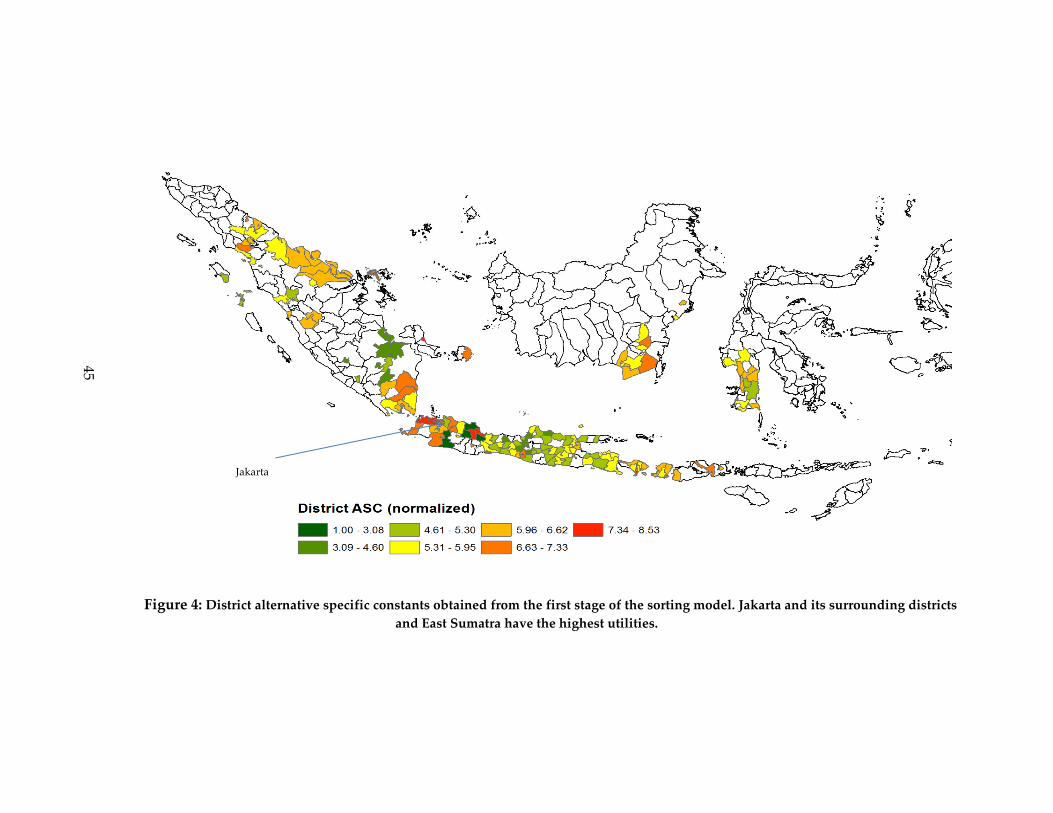
The other set of parameters arising from the first stage are the district fixed
effects and we depict them on a map (Figure 4). We see that Jakarta and its surrounding
districts have high level of ‘attractiveness’ and this is despite of its high housing prices
as seen earlier. Districts in East Sumatra are also relatively attractive possibly due to
their proximity to Singapore and Malaysia. In contrast, districts in the southern part of
Sulawesi have lower level of attractiveness relative to its expensive housing. Most
districts in provinces with more tropical forests and estate plantations, Sumatra and
Kalimantan, have relatively higher level of utility, although a few districts in the
southern portion of Sumatra are not as attractive.
22 Takeuchi et al. (2007) have similar findings from their study in Mumbai, India where slums dwellers place a premium to live near others of the same religion and language.

44
Table 5: First stage estimation results from the horizontal sorting model
(conditional logit model)
VARIABLES log(wage) 0.657***
(0.000) Location is in same province that respondent was at in 2000 (Yes = 0, No = 1) -2.620***
(0.000) Location is in same district in that respondent was at in 2000 (Yes = 0, No = 1) -3.190***
(0.000) Location is in same province in that respondent was at birth (Yes = 0, No = 1) -2.582***
(0.000) Location is in same district in that respondent was at birth (Yes = 0, No = 1) -3.048***
(0.000) Other religion*Proportion of other religion 1.984***
(0.000) Christian*Proportion of Christians 1.985***
(0.000) Muslim*Proportion of Muslims 1.435***
(0.000)
Households 10,125 Alternatives 174 p-value in parentheses *** p<0.01, ** p<0.05, * p<0.1
45
Figure 4: District alternative specific constants obtained from the first stage of the sorting model. Jakarta and its surrounding districts
and East Sumatra have the highest utilities.
Jakarta

46
1.6.1 Second stage results
Table 6 reports results from the second stage. Column (1) shows results from a
regular OLS without instrumenting for air quality. None of the district characteristics are
statistically significant, although most of them have the expected signs. The coefficient
for PM2.5 is small and highly insignificant, presumably because of a combination of
attenuation bias and omitted variables bias, where positive association between air
pollution and economic opportunities might pull the coefficient in opposite directions.
The instrumental variable strategy is reported in Column (2), with fire hotspots as
instruments in a two-stage least squares regression. The F-statistics from the first stage is
128.5, indicating strong correlation between the instruments and PM2.5. In the second
stage, air quality, crime index, and health facilities index are all significant at the 90%
significant level. Critically, the coefficient for instrumented PM2.5 variable is statistically
significant and negative at -0.079. This confirms that air pollution is a disamenity in this
context. When evaluated at the median PM2.5 level of 12 µg/m3, the MWTP is at about 1%
of income, a finding very similar to the 0.95% estimate (MWTP for PM10 , as percent of
income) in BKT.

47
Table 6: Second stage estimation results from the horizontal sorting model
(1) (2) (3)
OLS IV 1st stage IV 2nd stage
VARIABLES Adjusted
utility log(PM2.5) Adjusted
utility log(PM2.5) 0.007 -0.079***
(0.938) (0.000) Crime index -0.102 -0.299*** -0.129*
(0.260) (0.000) (0.053) Health facilities 0.026 -0.006 0.025
(0.168) (0.770) (0.105) Schools 0.020 0.008 0.021
(0.658) (0.848) (0.594) log(population density) -0.016 0.049* -0.013 (0.389) (0.069) (0.381) Fire hotspots from Southeast district > 50km away 0.004** (0.014) Fire hotspots from Southeast district > 50km away 0.005*** (0.004) Fire hotspots from South district > 50km away -0.002 (0.173) Fire hotspots from Southeast district > 50km away 0.002** (0.027) Constant 0.125 0.256 0.294***
(0.626) (0.143) (0.065) Province FEs Y Y Y F-statistics from 1st stage 128.5 p-value for Hansen J statistics 0.51 Observations 174 174 174 R-squared 0.472 0.233 0.066 p-value in parentheses *** p<0.01, ** p<0.05, * p<0.1

48
1.6.2 Comparison of MWTP
Next in Table 7, we make several comparisons of (i) the MWTP recovered from
the sorting model with
ii) another hedonic study in Indonesia, e.g. Yusuf and Resosudarmo (2009);
iii) and iv) two internal comparison with our datasets - property hedonic model
without air quality instruments, property hedonic model with air quality
instruments; and
v) re-estimating the sorting model without moving costs and religious
preferences.
Estimates from (ii) and (iii) suggest that people are willing to pay to be exposed
to more PM pollution. The most probable reason for this counter-intuitive result is
because air quality is endogenous in both cases and as predicted, there is an upward
bias in MWTP. To confirm this explanation, comparison (iv) shows that MWTP is now of
the expected sign when estimated using the property hedonic model combined with
instrumenting. However at $8.9 per year, it is lower than the MWTP found using the
horizontal sorting model ($12.6). One possible explanation is because the latter controls
for moving costs and religious preferences, i.e., for the possibility that the initial spatial
distribution of the population is correlated with the spatial distribution of air quality. To
check this explanation, comparison (v), re-estimating the sorting model excluding
moving costs and religious preferences, generates MWTP at $8.1 that is closer to

49
comparison (iii). In sum, these comparisons demonstrate how different judgments about
the structure of the choice influence the estimation of MWTP for air quality.
Table 7: Comparison of marginal willingness-to-pay for air pollutants
1.7 Welfare Analysis
The MWTP for improved air quality obtained in the prior section demonstrates
that residents in Indonesia are willing to pay for clean air but offers little in terms of
policy guidance. In contrast to conventional hedonic models, the main appeal of
structural models is that welfare effects (i.e., non-marginal changes in welfare) can be
estimated for counterfactual policy simulations by considering out-of-sample
predictions and re-optimization by agents (Sieg et al., 2004; Timmins & Schenkler, 2009;
Todd & Wolpin, 2010; Wolpin, 2007). This is especially valuable in situations of large-
Pollutant
MWTP to avoid 1 µg/m3 of pollutant
Time range
Source/Model
(i) PM2.5a $12.6 ($5.8, $20.7)
Annual
This study/Horizontal sorting
(ii) PM10 -$0.04 Yusuf & Resosudarmo (2010) / Property hedonic OLS
(iii) PM2.5b -$4.5 (-$5.7, -$3.4) This study/Property hedonic OLSc
(iv) PM2.5b $8.9 ($5.1, $12.6) This study/Property hedonic IVd
(v) PM2.5a $8.1 ($3.83,$ 11.2) This study/ Horizontal sorting without moving costs and religious preferencese
a Calculated using average wage of $1,260 and PM2.5 of 12 µg/m3
b Calculated using median rent of $54.4 and PM2.5 of 12 µg/m3
c See Appendix B for regressions results d See Appendix C for regressions results e See Appendix D for regressions results 95% confidence interval in parentheses

50
scale and unprecedented changes or policies. Using these models, policymakers can get
a first look at the possible implications of various scenarios.
To illustrate how this works, we consider a policy scenario that would lead to a
50% reduction in forest fires, an issue of considerable concern within and outside of
Indonesia because of regional and global externalities (e.g., Singapore and Malaysia).
The purposes of this exercise are twofold. First, we demonstrate how to utilize the
horizontal sorting model for welfare analysis of a policy outcome. Second, while we
cannot model the positive externalities for neighboring countries (such as Singapore and
Malaysia), we can show how even within Indonesia, positive externalities accrue to
districts where the policy will not affect directly.
The welfare measure used here is compensating variation, i.e., the willingness-to-
pay to hold utility at baseline level. Following Tra (2010, 2013) and Takeuchi et al. (2009),
the compensating variation is defined as:
(13)
CV in Equation (13) refers to the compensating variation that household i is
willing to pay for a change in air quality from X0 to X1, keeping utility at baseline. For the
sake of brevity, the other unchanging terms in the indirect utility function are
suppressed.
Two partial equilibrium welfare effects are presented here. First, we compute the
instantaneous welfare impact following changes in air quality. Second, we compute an

51
extended welfare change, allowing for second-order adjustments in wages and housing
prices to equilibrate observed and new expected population shares. While both
measures are based on equation (13), there is an important difference. For the
instantaneous change, we are simply inserting modified PM2.5 into the indirect utility,
while restricting mobility. For the extended welfare, we take into account that
households may choose new location following changes in air quality and thus we
adjust wages and housing prices to account for this.
For sorting models, the wage (or price) adjustment typically occurs in the
following way. The new PM2.5 prompts new optimal location choices, in turn changing
the expected population shares of each location (computed as the average logit
probability for each location for every household). These expected population shares can
be interpreted as labor supply and housing demand for each location (Timmins, 2005;
2007). Starting with labor, assuming that demand is inelastic or at least that the spatial
distribution of employers are fixed, in the short run wages will adjust such that the
expected shares equal the observed shares. That is, wages would increase in places
where the expected shares exceed the observed shares and wages will decrease in places
where expected shares are smaller than observed shares. This adjustment will iterate
until labor demand equals labor supply. A similar logic applies for adjustment of
housing price, assuming that housing supply is inelastic (e.g., Tra (2013); Klaiber and
Phanuef (2010)). Thus, the difference between the instantaneous and extended welfare

52
depends on the extent to which the expected and observed shares deviates. Clearly,
these assumptions about inelastic labor demand and/or housing supply will not always
be true, but our data does not give a satisfactory way of predicting how either would
change in response to the policy lever.23 Thus, both equilibrium welfare effects should be
interpreted as partial equilibrium or short-term changes. However, in spite of these
restrictive assumptions, it is important to present these results as the main benefit of
sorting models in policy analysis is that its ability to allow agents to re-optimize.
1.7.1 Brief background of air quality management in Indonesia
The Indonesian government is increasing its attention to air quality in urban
areas (Resosudarmo, 2002). For example, the Blue Sky program was launched in 1992
with the aim of reducing air pollution in five major Indonesia cities.24 The main target of
this program is vehicular emissions, with policies focusing on elimination of leaded
gasoline, use of low-sulfur diesel fuel, and use of smokeless fuel for two-stroke engines
(Ministry of Environment, 2011). However, policies for controlling another major source
of air pollution – forest fires in Indonesia – are scarce. At present, multiple decrees to
manage forest fires has been issued at the national level but lax enforcement and policy
gaps contributed to this problem continuing (Habitat, 2000). For example, there is lack
23 One fix is to follow Timmins (2005, 2007) , who collected the constants from individual location wage regressions and decomposes them into their constituents. This regression is then interpreted as labor demand. We cannot replicate this type of a fix as we do not have sufficient observations to run a wage regression at each location. 24 Description of the Blue Sky Program: http://projects.wri.org/sd-pams-database/indonesia/blue-sky-program-program-langit-biru

53
of coordination between local and federal government, which results in the local
government requiring permission from the central government before they can embark
on fire fighting. The delay incurred in getting federal government permission means
that an originally small fire is allowed time to spread and becomes more difficult to
control (Fatah & Udiansyah, 2009; Habitat, 2000). Thus, the Ministry of Environment
acknowledged that more needs to be done in order to reduce air pollution caused by
forest fires.25
1.7.2 Policy outcome scenario: Forest fires reduced by 50%
Forest fires have been the historical method for clearing land in Indonesia, but
they first received international attention only in 1982 as massive fires in East
Kalimantan destroyed 3.2 million hectares (about the size of Maryland) of tropical
forests (Fatah & Udiansyah, 2009; Gellert, 1998). Since then, the increased occurrence
and intensification of forest fires is receiving greater attention because neighboring
countries are affected by the smoke pollution and the global community has become
very concerned about the rapid shrinking in Indonesia’s tropical forests. As Indonesia is
in the tropical zone, this means that fires do not occur naturally or at least not at such
high frequency. The fires are often set by companies or individuals to clear forested land
for growing cash crops. Due to the high humidity and rainy weather for most parts of
25 Presentation by BAPEDAL (Ministry of Environment), 13 Dec 2006 (http://cleanairinitiative.org/portal/node/3387)

54
the year, these fires can only be sustained during the dry season from August to
November (Cochrane, 2003). Given the persistency of this problem, the Indonesian
government in 2002 placed combating forest fires as one of the country’s five top
priorities (Fatah & Udiansyah, 2009). Unfortunately, there has been very little economic
analysis of the welfare effects of the smoke reduction. 26
Thus, the purposes of this valuing a hypothetical policy outcome of 50%
reduction in forest fires are twofold. First, we wish to examine the welfare impacts of a
potential policy considered by the Indonesian government. Second, we wish to
demonstrate how to use a sorting model to value air quality policies. In principle, other
environmental policies, including other policies to change forest fires or PM2.5, can also
be examined using the model described in this paper.
To predict how fire hotspots affect PM2.5, a simple regression model is used
where district’s PM2.5 is regressed on its own count of fire hotspots and neighboring
districts’ fire hotspots count (Table 8). This regression specification is similar to the
construction of the PM2.5 instrument except for two differences. First, this simple
regression model includes the district’ own fire hotspots count. Second, neighboring
districts at multiple distances are used instead of at just one exclusion distance. The
reason for including more regressors is to gain as much explanatory power as possible.
26 To the author’s best knowledge, there are at least of couple studies valuing the economic impacts of the 1997 forest fires (Glover & Jessup, 1999; Tacconi, 2003). However, these studies are unsuitable for policy analysis as their results are only relevant to the particular event.

55
To address potential endogeneity concerns (e.g., fire hotspots are potentially correlated
with multiple factors such as precipitation which is negatively correlated with fires),
province fixed effects is included in the regression. Of course, remaining sources of
endogeneity, i.e., factors that vary at the district level and correlated with fire hotspots,
cannot be controlled for. As observed from the coefficients and significance level in
Table 8, a district’s air quality is most affected by fire hotspots in the district. Distance
plays a role as the impacts of distal districts’ fires reduces in both magnitude and
statistical significance as distances increase. The constant in this regression is 5.4 and this
represents the mean portion of annual PM2.5 unexplained by fire hotspots between
August to November and province fixed effects. In all, rather than an across the board
decrease in fire hotspots for all locations, we select only districts in North Sumatra, West
Sumatra, South Sumatra, South Kalimantan, and East Kalimantan (41 districts in all)
because these provinces (a) contain most of Indonesia’s tropical forest and oil palm
plantations and (b) are where most of the forest fires occur.
Table 8: Fire hotspots determinants of PM2.5 for policy scenario
VARIABLES PM2.5 Fire hotspots from own district 0.030***
(0.005) Fire hotspots from southeast district at 20km away -0.219***
(0.001) Fire hotspots from southeast district at 30km away -0.001
(0.658) Fire hotspots from southeast district at 50km away 0.001
(0.324) Fire hotspots from southeast district at 80km away -0.002

56
(0.158) Fire hotspots from south district at 20km away 0.224***
(0.001) Fire hotspots from south district at 30km away 0.004**
(0.025) Fire hotspots from south district at 50km away -0.001
(0.504) Fire hotspots from south district at 80km away 0.001
(0.459) Constant 5.406***
(0.000)
Province FEs Yes Observations 440 R-squared 0.901 p-value in parentheses *** p<0.01, ** p<0.05, * p<0.1 Standard errors clustered at province level
The gain in instantaneous welfare is $7.45 and extended welfare is $11.7 per
household annually (Table 9).27 The difference between instantaneous and extended
welfare can be rationalized as follows. The five provinces targeted for reductions in fire
hotspots are less populated than the other provinces. As such, when air quality is
improved in these places, there will be an increase in population towards these
provinces. To equilibrate population shares, this implies that wages will and housing
prices will decrease in the districts where there is out-migration and increase in districts
where there is in-migration. However, due to these price changes, there will be a second-
order optimization of locations which in turn prompts more price changes. Optimization
will stop once all households are in the location that maximizes their utility.
27 If this figure is aggregated by the total number of households, it will likely be a lower bound estimate as the welfare change only represent that of the decision-maker in the household.
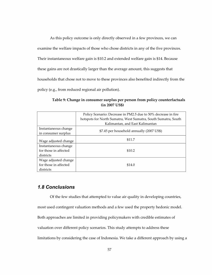
57
As this policy outcome is only directly observed in a few provinces, we can
examine the welfare impacts of those who chose districts in any of the five provinces.
Their instantaneous welfare gain is $10.2 and extended welfare gain is $14. Because
these gains are not drastically larger than the average amount, this suggests that
households that chose not to move to these provinces also benefited indirectly from the
policy (e.g., from reduced regional air pollution).
Table 9: Change in consumer surplus per person from policy counterfactuals
(in 2007 US$)
Policy Scenario: Decrease in PM2.5 due to 50% decrease in fire hotspots for North Sumatra, West Sumatra, South Sumatra, South
Kalimantan, and East Kalimantan Instantaneous change in consumer surplus
$7.45 per household annually (2007 US$)
Wage adjusted change $11.7
Instantaneous change for those in affected districts
$10.2
Wage adjusted change for those in affected districts
$14.0
1.8 Conclusions
Of the few studies that attempted to value air quality in developing countries,
most used contingent valuation methods and a few used the property hedonic model.
Both approaches are limited in providing policymakers with credible estimates of
valuation over different policy scenarios. This study attempts to address these
limitations by considering the case of Indonesia. We take a different approach by using a
58
structural horizontal sorting model of migration. In addition to directly tackling pitfalls
of the conventional hedonic model, estimation of economic welfare impacts of a specific
scenario illustrates how this framework can be used to conduct a range of policy
simulations.
We estimated MWTP for 1 µg/m3 of PM2.5 to be $12.6 (in 2007 US$). Critically,
this estimate is higher than the estimate from a conventional property hedonic model
(using the same data) and also higher than estimates from other hedonic studies of air
quality. We believe that correlation between air quality, population distribution and
economic activities may have biased previous estimates. First, to correct for correlation
in spatial distribution of population and air pollution, we explicitly model moving costs,
whereas the hedonic approach is are unable to take into account this important aspect of
household decision making (Timmins, 2005; 2007; BKT; Timmins & Schenkler, 2010). To
check this conjecture, we re-estimate the horizontal sorting model without moving costs
and the MWTP from this specification is downward biased and closer to the one from
the property hedonic model. Second, to address the negative correlation of air quality
and economic opportunities, we develop and use a wind- and distance-based
instrument – using location of forest fire hotspots upwind from population
concentrations. Without instrumenting for air pollution, it would seem as though
Indonesians are willing to pay to be exposed to more air pollution.

59
A useful feature of structural models is the ability to estimate welfare effects of
policy counterfactuals. We consider a scenario where forest fires are reduced by 50% in
five provinces and present two partial equilibrium welfare changes – an instantaneous
effect and a wage-adjusted effect. The immediate welfare change is $7.44 and the wage-
adjusted welfare is $11.7 per household annually (in 2007 US$).
To put the welfare estimates in perspective, we should consider other costs and
other benefits of such a policy. Although the sorting model allows us to consistently
measure the benefits to households, it is not a general cost-benefit tool. Instead, here we
discuss some of other costs and benefits. Oil palm plantations are critical to Indonesia
(Tan-Soo et al., forthcoming), and therefore any moratorium on forest fires and air
pollution control is likely to impose large costs on this sector. On the benefits side of the
ledger, Indonesian air pollution imposes negative externalities as their neighboring
countries of Singapore, Malaysia, and Brunei. Further, forest fires are part and parcel of
rampant tropical deforestation. Ferraro et al. (2012) provide the latest systematic review
of ecosystem services (e.g., carbon sequestration, pollination, human health, ecotourism,
hydrological services) from reduced deforestation.
Because air-pollution imposes very large health burden in developing countries,
we must reconsider policies to improve air quality. This study contributes to this
attempt by valuing air quality in Indonesia. We show that Indonesians’ MWTP of
improved air quality, at about 1% of annual income, is comparable to developed
60
countries. This suggests that developing countries should step up in their efforts to
consider air quality management policies. While Indonesia appears to be moving in this
direction as they recently agreed to set national PM2.5 standards, many other developing
countries are still slow to implement and enforce standards for air pollutants. Results
from the policy scenario also show there may be externality gains within the country.
This suggests that cost-benefit analysis for air quality policy should include these
externalities to ensure a full accounting of the benefits.

61
2 Impacts of early-life exposure to forest fires on long-term outcomes of Indonesian children
2.1 Introduction
There is increasing recognition that peoples early-life environment is correlated
with their adult health outcomes, especially since Barker (1990) artfully synthesized
evidence from the vast epidemiological literature to popularize the “fetal and infant
origins” hypothesis. Multiple studies have since attempted to test this hypothesis,
including in economics. These studies showed that exposure to various early-life shocks
have lasting repercussions in a wide range of latter-life outcomes such as cardiovascular
diseases, respiratory systems, cancers, psychiatric illnesses, height attainment, earnings,
employment type, and cognitive ability (e.g., Sallout & Walker, 2003; Currie & Vogl,
2014; Almond, 2006; Mancini & Yang, 2009). Such studies have potentially large policy
implications. First, to the extent we can mitigate and/or adapt to ‘shocks’, these findings
add a new layer of irreversible, if not sizable costs to any inaction. Second, many of these
health and socioeconomic outcomes are already targeted by interventions and more
effective interventions can be designed if the causal links between early-life shocks and
latter-life outcomes are clarified. For example, Bhradwaj et al. (2014) showed that
exposure to carbon monoxide has a sizeable impact on school examination results and
thus an alternative policy to improve test scores could come through the channel of
controlling outdoor air pollution.

62
While this literature proliferated in developed countries due to data availability
and interests of the policy research community, a very small literature from developing
countries is only surfacing recently. Currie and Vogl (2014) argued that more of such
studies are needed for low-income countries due to higher frequency and intensity of
‘shocks’. . However, the challenges of conducting such studies in developing countries
are twofold. First, reliable data on exposure to shocks is lacking because there are very
few data sets that contain detailed individual data over multiple periods, which include
for example respondents’ birthplace and their exposure history. Second, even if
information on exposure is available, it is also important to obtain data on parental
inputs, such as their biological outcomes and their nurture and care, which depends on
socioeconomic status and access to public services.
Thus, we contribute to this literature by investigating the long-term health
impacts of an air quality shock, resulting from the biggest recorded fires in Indonesia’s
history (Heil & Goldammer, 2001). This event in 1997 prompted several studies
assessing its impacts, but all looked at its contemporaneous impacts. Thus, this paper
makes several potential contributions to the literature. First, in response to Currie &
Vogl (2014), this is one of the first studies to show evidence of the impacts of early-life
exposure to air pollution in developing countries. Unlike other studies, we use a variety
of health and cognitive indicators and demonstrate that adverse impacts are found in
most outcomes we investigate, especially indicators of long-term health. Second, this
63
study feeds into the broader topic of cost-benefit analysis for air quality management
policies by documenting evidence on an ignored benefit. As air pollution is often
correlated with economic growth, this necessitates a tradeoff between increasing
economic opportunities and managing the associated health burden. Third and related,
it is timely to conduct this study as air pollution is receiving recognition as a major
source of health burden. Just recently, the WHO doubled their estimates of air pollution-
related mortality due to increasing evidence that damages were previously understated
(WHO, 2014). In this regard, this study adds to the evidence pool on the health damages
caused by air pollution. With worsening air quality in many developing countries, it is
likely that this topic will only increase in significance in the future. Fourth, we expand
the evidence base in another dimension by examining forest fires, whereas most studies
focus on industrial and vehicular emissions. This is also relevant for policy because
forest fires in tropical countries such as Brazil and Indonesia are regular events and have
global implications in the form of carbon emissions and biodiversity. Furthermore, there
is a reinforcing feedback with global climate change as these forest fires, while set by
humans, can only be sustained in dry seasons. There is already evidence that changing
weather patterns have intensified dry seasons in Indonesia, which thus increase the
frequencies of forest fires (Timmermann et al., 1999; Yeh, et al., 2009). Lastly, these
results also contribute to an ongoing puzzle where catch-up growth is observed in some
studies (Rabassa et al., 2012; Tiwari et al., 2013; Adair, 1999) while not in others

64
(Cameron et al., 2005; Martorell et al., 1994; Hoddinott & Kinsey, 2001; Mancini & Yang,
2009). The policy implications will be vastly different if catch-up growth are appreciable
and can reverse initial setbacks.
We identify approximately 700 children from the Indonesian Family and Life
Surveys (“IFLS”) who were in-utero at the time of the 1997 Indonesian fires. Because
these children were at different proximities to the smoke and fire hotspots, we can
examine the relationship between variation in air quality and various child health
metrics. Exploiting variation in time of birth and location of birth, we can isolate the
influence of air quality while holding constant these district level fixed effects. We find
that a child if exposed at the mean air pollution level during early-life is about 3-4
centimeters shorter, perform worse in a cognitive test, and have decreased lung capacity
compared to his/her unexposed peers 10 years after exposure. As growth rates largely
stabilized by age three (Martorell, 1995; 1997; Martorell, et al., 1994), this means that
observed impact at age 10 is likely to persist into adulthood. In a developing country
setting, the findings for height is bad news as there is robust evidence that an adult’s
height (as a proxy for various drivers) is correlated with socioeconomic outcomes such
as wages and educational attainment (Strauss & Thomas, 1998).
Unpacking the main findings by subgroups of exposure, shows that exposure at
the first trimester is most harmful for height attainment and cognitive ability, while
exposure at second and third trimester is most harmful for lung functions. These results

65
while interesting are tentative as our sample is not large enough to precisely identify
effects at this fine level. Also, while we know that prenatal exposure to air pollution is
harmful to the fetus, the trimester specific mechanisms is still to be determined (Moore
& Persaud, 2011). 2.1 A very long subsection title to illustrate line spacing in the
document and in the table of contents (yes, single spacing for headings)
2.2 Background
The 1997 forest fires are the largest recorded in Indonesia (Siegert et al., 2001).
Fires started as early as May/June and peaked towards September and October before
being slowed down by the monsoon arrival in November (Heil & Goldammer, 2001). In
the aftermath, these fires burned through 9.8 million hectares of forests and peat
swamps and caused global carbon emissions in 1997 to spike by about 40% from average
levels (Page, et al., 2002). The causes are a combination of anthropogenic and natural
events. First, unlike their temperate counterparts, tropical forests do not require fire to
regenerate (Cochrane et al., 1999). Also, spontaneous fires are rare as precipitation and
humidity is high throughout the year in tropical climate. In Indonesia, there is a small
window of dry season from around August to October where rainfall is low and thus
forest fires can be sustained (Stolle et al., 2003). This dry season was especially intense in
1997 as the El Nino Southern Oscillation weather phenomenon that year was
particularly intense (Page et al., 2002). Using fires to clear forests is a traditional practice
in Indonesia for a group of people known as shifting cultivators (Angelsen, 1995). This

66
nomadic group typically clears a small plot for self-subsistence agricultural purposes
and will migrate once that land becomes infertile. However, it is unlikely that the
shifting cultivators are solely responsible for massive fires as it has become obvious that
plantation owners are also using fires to clear land (McCarthy, 2001). While there is no
conclusive evidence to show the extent which group is responsible for the 1997 fires,
increased monitoring in recent years show that the plantation owners are assuming most
of the blame (Obidzinski et al., 2012; Germer & Sauerborn, 2008). The unprecedented
magnitude of these fires generated global attention on this issue and has since sparked a
series of studies assessing the health and economic impacts caused by air pollution (e.g.
Frankenberg et al., 2005; Sastry, 2000; Emmanuel, 2000; Jayachandran, 2009).
The link between early-life health insults and adult health is as follows. Early-life
(defined as the period from fetal life to about two or three years of age) health insults
affects early-life health which are often identified as low birthweight, short gestation
period, or intrauterine growth restriction (Maisonet et al., 2004). These early-life health
conditions may persist into adulthood if the body is unable to catch-up. One strand of
studies focuses on these individual links (e.g. Bobak, 2000). That is, either between early-
life health insults and early-life health or between early-life health and adult health.
Most of these studies tend to take place in developed countries where information on
early-life health is more reliable (mostly through hospital records) and more readily
available. In particular, there is a thriving literature that investigates the link between in-

67
utero exposure and fetal growth. Maisonet et al. (2004) and Glinianaia et al. (2004)
reviewed studies in this literature and both concluded that there is evidence of air
pollution being associated with poorer fetal health although the impacts are small
compared to other pollutants.
Another strand uses a reduced-form approach to directly examine the
relationship between early-life health insults and adult health or socioeconomic
outcomes (e.g. Mancini & Yang, 2009). The approach allows the researcher to sidetrack
the lack of early-life health data and is especially useful for developing country settings
where information on early-life health is generally unavailable but where environmental
threats are formidable. Moreover, this approach is more suitable if the study’s objective
is to examine the economic impacts of early-life exposure as most economic impacts
tend to be fully manifested in adult life. .
Broadly speaking, there are two identification strategies for estimating the
impacts of environmental health insults (proxied by environmental shocks in most
cases). One relies on a single catastrophic event to proxy for health insults and this is the
approach used in this study. The rationale is that these events are rare, unpredictable,
and have large impacts. Thus, it is unlikely that one can plan to mitigate or adapt for
these events, especially at the onset. For example, mortality estimates from the great
famine of China ranged from 15 million to 45 million deaths (Riskin, 1998). Empirically,
this means that causal inferences arising from these events are easier to justify.
68
Interpretation is also straightforward as one is either exposed or unexposed to these
shocks. On the flip side, the scarcity of catastrophic events limits the proliferation of this
strategy and this makes it difficult to generalize the results to other settings and use in
public health planning affecting daily life. Moreover, causal identification may be
threatened especially if the ‘shock’ persists for a long time as more resourceful victims
can migrate or find other means to adapt.
Famines are commonly used as ‘shock’ event due to their rarity (in a particular
location) and because the channel of low nutritional intake at early stages of
development is better understood medically (Wells, 2003). Some examples are the 1949-
1951 great famine in China (e.g. Chen & Zhou, 2007; Almond et al., 2010; Fung, 2009, the
1984 Ethiopia famine (Dercon & Porter, 2014), and the Dutch potato famine of 1846-1847
(Lindeboon et al., 2010). Other than famines, pandemics (e.g., Almond, 2006; Nelson,
2010) and wars (e.g., Akresh & de Walque, 2008; Akresh et al., 2011) have also been used
although the channels and mechanisms are not always obvious. All of these studies
except for Fung (2009) found evidence either in the form of decreased height, earnings,
educational attainment, or labor capital following early-life exposure to these adverse
shock events. Fung (2009) in contrast found that those exposed are likely to be obese
during adulthood. This is in line with some findings from the medical literature which
shows that catch-up growth can lead to obesity (Ong et al., 2000).

69
On the other hand, another empirical approach is to utilize ‘shocks’ in everyday
phenomenon. Rainfall is one of more commonly used environmental factors in this
approach as there are numerous accounts of precipitation playing a significant role in
the livelihood of those in agricultural communities (Kochar, 1995; Jacoby & Skoufias,
1997). Mancini and Yang (2009) measure deviation of rainfall from the mean amount and
use this difference to represent shocks. They applied this strategy to the Indonesian
context and found that females born during years of low rainfall tend to be shorter and
have lower educational attainment in adulthood. Conversely, no effects were found for
males and they attributed this to gender inequality in household allocation of resources.
Tiwari et al. (2013) and Rabassa et al. (2012) similarly exploited rainfall deviation in
Nepal and Nigeria to assess children’s height. Moreover, they attempted to distinguish
between income effects and effects of worsened disease environment by introducing
additional years of rainfall shocks. In contrast to Mancini and Yang (2009), they found
that health damages caused by rainfall shocks are transitory as affected children quickly
recover to be on par in height with their peers by the year after the shock. A direct
empirical benefit of interpreting deviations from mean as shocks is that we need not rely
on catastrophic events. For example, the three studies cited here relied on yearly
deviations and thus this enlarges their sample size and also increases the possibility of
study sites. However, causal identification is weaker as while rainfall fluctuation is
unpredictable to the researcher, but may be anticipated by locals and can respond in

70
such. For example, Timmins (2007) showed that Brazilians’ choice of location is partly
determined by climatic factors such as temperature and precipitation. Bohra-Mishra et
al. (2014) also showed using data from Indonesia that migration is induced by climatic
variation rather than in response to disasters.
Up till now, there are only a handful of studies that looked at the long-term
impacts of early-life exposure to air pollution, either in developed or developing
countries. Sanders (2012) used an instrumental variable strategy to obtain exogenous
shifts in air pollution in the United States. He found that increased early-life exposure to
total suspended particulates is associated with poorer test performances in high school.
Under a similar context, Isen et al. (2013) examined the relationship with adults’
earnings. They found that increased early-life exposure is associated with decreased
earnings. Morales et al. (2014) in a study conducted in Spain found that exposure to NO2
and benzene at the second trimester is more likely to be associated with decreased lung
capacity at age 4.5. The only developing country paper on this topic comes from
Bharadwaj et al. (2014) who examined this question in the Chilean context.28 They found
that test score at 4th grade is negatively associated with increased carbon monoxide
exposure in the third trimester. In all of these cases, the air pollution level is much lower
than those experienced in the 1997 fires and most of the dirtiest cities in Asia.29
28 The tine period at which the study is conducted was at a time when Chile was still a developing country. 29 For example, the highest air quality index (AQI) recorded in Bharadwaj et al. (2014) is around 75+ whereas the AQI for the most polluted day during the 1997 fires is out of range.

71
Less clear from all these studies are the mechanisms of how air pollution affects
health (Boback & Leon, 1992). What is known for sure is that different air pollutants
affect the fetus in different ways. Perhaps the best studied air pollutant is carbon
monoxide which is known to restrict body’s intake of oxygen and it can also directly
crossover to the placenta (Longo, 1977). Put together, this may result in reduced oxygen
intake for the fetal, thus hampering development (Ha et al., 2000). Other air pollutants
are not known to be able to directly affect the placenta, but may still indirectly affect by
increasing blood viscosity in the mother, and this in turn will cause adverse birth
outcomes (Peters et al., 1997; Bouthillier et al., 1998; Knottnerus et al., 1990; Ha et al.,
2000). Similarly, evidence on the economic mechanisms is thin, but growing.
Frankenberg et al. (2005) found that Indonesian haze (air pollution from forest fires)
adversely impact the physical functioning of prime-aged women. Hanna and Olivia
(2011) found that working hours or labor capital increased after air quality improved
because a power plant was shut down in Mexico City. Chang et al. (2014) also found that
productivity at a pear packaging plant is correlated with daily ozone levels in Southern
California. Hence, a possible economic mechanism is that exposure to air pollution
reduces adults’ ability to work and this results in reduced nutritional intake. This
channel could play out stronger in a developing country as savings are low and most
people rely on physical work (Edwards, 1995). Direct evidence of air pollution harming
infant health can also be found in Jayachandran (2009) who found using that the 1997

72
Indonesian forest fires caused a mortality rate of about 1.2% of the birth cohort. Other
studies covering the same event also showed that adult mortality and morbidity
increased as a result of increased air pollution (Sastry, 2000; Emmanuel, 2000).
A final but intriguing mechanism is epigenetics. The basic idea is while our
inherited gene structure is unchangable, but our environment could alter how the gene
is expressed (Gicquel et al., 2008). This is a relatively new discovery in biological
sciences, but the potential it has in answering important questions about disease
formation has prompted a new field of study. The impacts are potentially profound as
researchers have found the role it plays in various diseases such as inflammation,
obesity, diabetes, and cardiovascular diseases (Choi & Friso, 2010). One of main
channels where epigenetics is obvious is in developmental or fetal programming
(Gicquel et al., 2008). The idea is that the fetus will receive signals about the outside
environment and develop in response to adapt to postnatal life (Gluckman et al., 2007;
Gluckman & Hanson, 2004; Bateson et al., 2004). For example, the ‘thrifty genotype’
hypothesis speculated that fetus that received less than adequate nutrition will program
the body by increasing capacity to store fats to be prepared for an undernourished
environment outside of the womb. However, our knowledge on the role of epigenetics
in fetal development and the impact of various types of stresses is still extremely
rudimentary (Morgan et al., 2005).

73
2.3 Framework
The theoretical model employed here takes after the familiar health production
function introduced by Grossman (1972). Essentially, health is a stock variable and a
function of multiple inputs at the individual and community level:
(14)
is child i outcome at time t and is a function of the initial endowment and
outcomes at earlier time periods which are represented by inputs at the household level
such as nutrition and childcare ( ), and inputs at the community level such as exposure
to pollution ( ). The initial endowment takes a slightly different representation:
(15)
The main difference to this expression is E, which are the genetic inheritance
from the parents. The subscript 0 in I and C represent the inputs received during the
early-life period. Depending on whether the specific outcomes are measurement of long-
term health or short-term biomarkers, the importance of early-life inputs differ
accordingly. For example, height being a measurement of long-term health means that

74
early-life inputs should matter more.30 On the other hand, weight fluctuates according to
short-term conditions and so recent inputs should matter more.
As the purpose of this study is to estimate the long-term implications of early-life
exposure to air pollution, we can combine equation (14) and(15) to estimate its reduced-
form empirical counterpart:
(16)
In this setup, the j subscript refers to the birth district of child i and the 0
subscript refers to the month and year at which the child is born. The coefficient of
interest is which measures the marginal impact of air quality which the child was
exposed to during in-utero or first six months of life. This coefficient is identified by
variation in the birth month and birth location of the child. I is a vector of parental
inputs consisting of parent’s education attainment and genetic contributions to the
child’s outcome (either height, weight, or lung capacity,). are a set of fixed effects for
the month of birth and will control for month-specific effects such as seasonal weather
patterns that also affect long-term health outcome (Mancini & Yang, 2009; Tiwari et al.,
2012; Rabassa et al., 2013). Lastly are a set of districts’ fixed effects that controls for
any locational factors that may affect long-term health outcomes such as local nutrition
30 “Child growth indicators and their interpretations” (http://www.who.int/nutgrowthdb/about/introduction/en/index2.html)

75
programs, health facilities quality, and etc. For example, the quality of health facilities
may be correlated with levels of AQ, particularly because of the way the joint data set of
health outcomes, parental inputs, and environmental quality is merged, thereby
potentially confounding the effects of AQ.
Estimation of could be biased due to various endogeneity issues. First, Tan-
Soo (2015) showed that locational sorting at the district level indeed occurs along the
lines of air quality in Indonesia. One way to deal with this endogeneity is to find an
exogenous source of variation, using forest fire hotspots and wind direction as
instruments as in Tan-Soo (2015). However, data for forest fire hotspots began from 2001
and thus prevents the use of such strategy in this study. The threat to identification in
this instance is that those in lower socioeconomic status may choose to live in places
with worse air quality and thus any observed adverse health impacts could be wrongly
attributed to air quality. However, given that forest fires were still not as common in
1997 and that the 1997 fires were exceptionally large, it is unlikely that behaviors were
planned with fires of this magnitude in mind.31 Jayachandran (2009) and Frankenberg et
al. (2005) investigated migration patterns and found that there were no abnormal short-
term or long-term migrations before or after the 1997 fires. A comparison is also made
by showing the spatial distribution of air quality in October 1991 and 1997 (Figure 5).
31 The previous fires were in 1991 (199,000 ha) and 1994 (406,000 ha) and were small compared to the 1997 fires (9,700,000 ha) (Makarim & Deddy, 1997; .BAPPENAS, 1999)

76
There were forest fires during this month in both years, however it is clear from the
figure that more places were affected and at a higher level in 1997.
Second, air quality is measured by a satellite-derived dataset. While ground-
proofing has demonstrated the viability of this data source, it is possible that air quality
is still measured with error. Hsu et al. (1999) showed that the error structure is classical
and so the bias caused by measurement errors will induce the coefficient towards zero,
hence providing more conservative estimates, that is, attenuating the magnitude of the
impacts.
Third, although there is evidence to show that air quality and economic
opportunities are inversely correlated (e.g. Heutel & Ruhm, 2012; Chay & Greenstone,
2007; Tan-Soo, 2015), it is possible in this particular context that the reverse is true
instead. For example, tourism revenue was lost as many flights were canceled during
the period of the 1997 fires (Glover & Jessup, 2006). Such economic disruptions may
affect livelihood and thus nutritional intake of pregnant mothers or young children.
Towards this end, we included district fixed effects to control for any decreased
economic opportunities that did not vary at the month level. Obviously then, any
decreased economic opportunities that vary at the month level and is correlated with air
quality will confound our estimates.
Fourth and related, the air quality assigned to each child is based on his/her time
of birth and location of birth. Hence, the effects of air quality will be confounded if there

77
are any unobserved attributes that similarly vary at the same spatial-temporal scale. For
example, there could be seasonal effects at each location. To correct for this, we repeat
the analysis on cohorts born before and after the fires, but are assigned exposure to air
quality as though there were born in 1997/1998. For cohort born after the fires, we expect
air quality to not have any impacts on their outcomes. For the cohort born before the
fires, while it is demonstrated that air pollution is a leading cause of mortality, impacts
on our outcomes of interest is mostly understudied.
Lastly, household’s inputs could be correlated with air quality exposure in two
ways. First, as mentioned earlier, household’s choice of location could be a signal of their
socioeconomic status (“SES”) where poorer households live in more polluted areas. In
turn, their lower SES may be correlated with other households’ inputs that also affect
child’s outcome. Second, it is also possible that parents may compensate for child’s
growth if they notice their child is falling behind in height or other areas. As both
behaviors act in opposite directions of their correlation with exposure to air pollution
and outcomes, it is difficult to predict the direction in which the coefficient will be
biased. To test for them, we included in a specification households’ adoption of
improved sanitation and non-biomass fuel at different time periods.
2.4 Data
This study consists of two main datasets: household and air quality. The
household data come from the longitudinal Indonesian Family and Life Surveys

78
(“IFLS”). We use data from rounds conducted in 1997, 2000, and 2007. We select children
who are in-utero or in the first six months of their lives at any time between August to
October 1997.32 This empirical strategy is essential to exploit the ‘shock’ in air quality
caused by the 1997 fires, without attempting to model health more generally considering
the universe of children whether they were in-utero or not. An alternate empirical
strategy is to define shocks as ‘deviation from mean’ such as Mancini and Yang (2009)
and consider all individuals whose birth location and AQ exposure level at early-life can
be tracked. While this would enlarge the sample size, it may introduce bias induced by
households sorting along the lines of air quality variation as suggested by Boshra-
Mishra, et al. (2014) . As explained below, we also compare with somewhat older and
somewhat younger kids to examine the early-life exposure hypothesis.
For those in-utero, we assume that they went through a gestation period of 10
months.33 This downside to this assumption is that there are evidence showing that one
of the effects of fetal exposure to air pollution is preterm delivery (Maisonet et al., 2004).
However, the effects on preterm delivery are small and a robustness check of assuming
a nine month gestation period is conducted to ensure that results are not spurious.34
Children’s birthplace is then obtained from the child’s mother location in the 1997
32 The final sample used for estimation is smaller than 1,303 due to various missing covariates. 33 A full-term delivery is medically defined as 37-42 weeks whereas preterm is defined as earlier than 37 weeks. 34 See Error! Reference source not found. & Error! Reference source not found..

79
survey.35 Using this location, we can assign air quality measurement for their period of
exposure which is defined as the average of the months they are in-utero or in the first
six months of life between August to October 1997. For example, a child born in
December 1997 is in-utero for all three months and thus exposure is defined as the
average air quality from August to October.
As ground air quality stations are rare in Indonesia, we rely on satellite-derived
data to proxy for air quality. The proxy used here is Aerosol Index (“AI”) which is
detected using the Total Ozone Mapping Spectrometer (“TOMS”) instrument installed
on satellites. The relevant satellite for the 1997 period is the Earth Probe satellite which
takes about 200,000 daily measurements covering all spots on Earth except near the
poles (TOMS Science Team, 2015). The TOMS instrument was originally designed to
measure atmospheric ozone levels, but has been used to measure the relative amount of
aerosols in the atmosphere (Lee et al., 2009). These aerosols include dust, volcanic dust,
and smoke. AI readings are highly useful for researchers in developing countries as
there are many places without ground measurement stations. Frankenberg et al. (2005)
and Jayachandran (2009) also used AI as proxy for air quality in their studies in
Indonesia. Attempts to ground-truth AI with station measurements shows a high
percentage of agreement for air pollution created by forest fires in Africa and Latin
America and any remaining errors are of the classical-type (Hsu et al., 1999). To the
35 IFLS does not record birthplace if the respondent is less than 15 years old at the time of survey.
80
extent classical measurement errors is a problem in this case, this would cause
attenuation bias in our estimates.
AI is measured on 1 degree by 1.25 degree grids (1 degree is approximately 50km
at the equator and progressively larger as we move away) and varies at the monthly. We
then overlay these grids on Indonesian districts. The AI assigned to each district is the
average of the grids that the district overlapped Figure 5 shows variation in AI for each
of the three months we are considering. There are some locations where AI is
consistently high, such as Sumatra and Kalimantan. However, there are also parts of
Java where AI is high in August, but receded in October.
Temperature and precipitation data are included as controls due to the high
correlation between climatic factors and air quality (Aufhammer et al., 2013). These
variables are satellite-derived as well with rainfall being obtained from the Global
Precipitation Climatology Project and temperature from the Global Historical
Climatology Network.
Table 10 displays the summary statistics. First, the outcome variables consist of
height-for-age z-score (“HAZ”), weight-for-age z-score (“WAZ”), results of a cognitive
test administered by the IFLS, and lung capacity. HAZ is chosen as an outcome because
of its ability to proxy for future SES and also because height is a good measurement of
long-term health. WAZ, on the other hand is used as a ‘counterfactual’ outcome as
weight respond more rapidly to contemporaneous conditions and thus we do not expect

81
prenatal exposure to air pollution to affect weight at later life. Lastly, cognitive test
results and lung capacity are both included to provide a more detailed examination of
how air pollution affects health.

82
Figure 5: Variation in aerosol index across August, September, and October
1997. Severity of AI increases from dark green to red shades.
August
October
September

83
The average HAZ is about -1.57. This negative average suggests that compared
to a reference group in the United States, Indonesian children are short.36 Similarly, the
average WAZ is also negative at -1.54. However, the choice of reference growth
standards will not bias results because each level of exposure has the same adjustment –
i.e., there is no systematic bias. The lung capacity (as measured using a puff test)
averaged at around 183.2 ml. There is large variation in lung capacity as this varies
widely along age and gender. The variable ‘correct patterns’ refers as the percentage of
answering correctly cognitive questions on patterns recognition. There are 12 questions
in all and the average score is around 69%.
Next, the mean AI exposure is 0.1 and there is significant variation as the lowest
is 0 and maximum is 0.32. As the AI is a unitless construct, it is best understood as a
value of 0 indicating crystal clear skies and a value of 0.4 indicates barely able to see the
mid-day sun. We further investigate AI using two sets of histogram.
Table 10: Descriptive Statistics
Variable Obs Mean Std Dev Min Max
Height-for-age z-score 829 -1.57 1.15 -4.53 2.13
Weight-for-age z-score 825 -1.54 1.35 -4.92 4.24
Lung capacity (ml) 838 183.16 47.18 90 420.67
Cognitive test results 867 0.69 0.23 0 1
Aerosol index 898 0.1 0.04 0 0.32
36 FAO produced a table showing how average children height in each country compares to different centiles of the United States growth standards. The table shows that average Indonesians’ height hovers at around the 5 percentile level (http://www.fao.org/docrep/MEETING/004/M2846E/M2846E07.htm).

84
Precipitation (mm) 898 22.07 18.47 0.63 138.32
Temperature anomaly (oC) 898 -0.19 0.27 -0.82 0.95
Improved sanitation in 1997 (1 = yes;
0 = no) 723 0.69 0.46 0 1
Biomass fuel in 1997 (1 = yes; 0 = no) 725 0.46 0.5 0 1
Improved sanitation in 2000 (1 = yes;
0 = no) 854 0.73 0.44 0 1
Biomass fuel in 2000 (1 = yes; 0 = no) 854 0.32 0.47 0 1
Male (1 = yes; 0 = no) 841 0.53 0.5 0 1
Father’s height (cm) 802 161.15 10.99 15.6 182
Mother’s height (cm) 846 150.31 8.48 15.4 166.4
Father’s weight (kg) 802 58.95 11.02 3.8 104.1
Mother’s weight (kg) 846 55.29 11.31 4.3 108.8
Father’s lung capacity (ml) 800 403.03 94.96 113.33 743.33
Mother’s lung capacity (ml) 844 279.71 60.9 96.67 473.33
Father at least high school (1 = yes; 0 =
no) 841 0.26 0.44 0 1
Mother at least high school (1 = yes; 0
= no) 846 0.22 0.42 0 1
Figure 6 and Figure 7 shows the distribution of AI by years and months
respectively and we can see the distribution of AI is generally similar across months and
years. A scatterplot of HAZ against early-life exposure to AI shows a slightly negative
relationship (Figure 8). The basis of this relationship may however change as more
controls are added.
Average precipitation is around 22 mm and this is lower than usual due to the
months of August to October being drier months. Temperature is measured as
anomalies from historical averages and the average anomaly is actually lower than the
historical average by around -0.19 degrees Celsius. This is perhaps unsurprising as the

85
main climatic factor supporting forest fires is lack of rain rather than temperature
variation.
Average parents’ heights are 1.6 meters and 1.5 meters for father and mother
respectively in Indonesia. Fathers are generally heavier than mothers at 59 kg compared
to 55.3 kg. Average lung capacity is much larger for fathers (403 ml) compared to
mothers (280 ml). For schooling attainment, we see that about 26% of fathers completed
high school while 22% of mothers completed high school. For household inputs, we see
that about 46% of children live in households using biomass fuel in year 1997 and this
decrease to about 32% in year 2000. Similarly, the proportion of children living in
households using improved sanitation facilities increased from 69% in year 1997 to 73%
in year 2000.
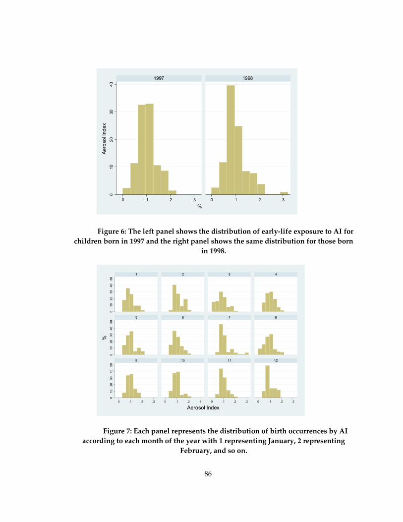
86
010
20
30
40
0 .1 .2 .3 0 .1 .2 .3
1997 1998
Aerosol Index
%
Figure 6: The left panel shows the distribution of early-life exposure to AI for
children born in 1997 and the right panel shows the same distribution for those born
in 1998.
010
20
30
40
50
010
20
30
40
50
010
20
30
40
50
0 .1 .2 .3 0 .1 .2 .3 0 .1 .2 .3 0 .1 .2 .3
1 2 3 4
5 6 7 8
9 10 11 12
%
Aerosol Index
Figure 7: Each panel represents the distribution of birth occurrences by AI
according to each month of the year with 1 representing January, 2 representing
February, and so on.

87
Next, Figure 8 shows the breakdown of the births by months and years. One
concern is that the air pollution may increase preterm births. To check for this, we
graphed births’ distribution by month for other years. In comparison, we see that there
is no spike for the latter months in 1997 and no deflation for the early months in 1998.
This is consistent with evidence from the medical literature suggesting that the impact of
air pollution on preterm birth is small in magnitude.
-4-2
02
Height-for-age z-score
0 .1 .2 .3Aerosol Index
Figure 8: Scatterplot of HAZ against early-life exposure to AI.
2.5 Results
Table 11 contains results of estimation of equation (16) with HAZ as outcomes to
illustrate how the AI coefficient changes with each specification. Column (1) shows the
result of a basic pooled-OLS with only parents’ height and month of birth fixed-effects

88
as controls. The purpose of presenting results from this regression is to serve as a
comparison with other specifications. The effect of 1-unit exposure to AI during in-utero
or first six months of life is 2.4 standard deviations in height differential at ten years old.
As AI ranges from 0 to 0.3, a 1-unit change is not a meaningful comparison. Rather, a
more useful interpretation to assess the height differential at the mean level of AI
exposure which is at about 0.1 relative to being unexposed (i.e., AI = 0) In this regard, the
height differential is 0.24 standard deviations or about 1.6 cm according to the growth
chart in which the HAZ were calculated.37 Adding district fixed-effects makes a sizeable
difference as height differential increased to about 2.8 cm at the mean level of exposure.
A plausible explanation is that children located in more polluted districts also have more
resources to mitigate the effects of dirtier air – that is, without this separation of the air
pollution and social (resource) effect, the negative impact of pollution was confounded.
This is consistent with our understanding that places with more economic opportunities
tend to be more polluted (Chay & Greenstone, 2005; Heutel & Ruhm, 2012). Next,
parental educations are added as there are evidence showing that parents’ education
levels are strong determinants of children’s height (Thomas et al., 1991; Thomas, 1994).
Two educational binary variables (father’s and mother’s high school attainment) are
added to the regression and thus its coefficients should be interpreted with respect to
37 The actual height differential in centimeters depends on the gender, age, and percentile of the child. The example used in the text refers to the male child at 120 months on the 50 percentile of the height-for-age chart.

89
the excluded categories. Magnitude of AI coefficient increased by about 33% (equivalent
to a 3.8 cm height differential at the 0.1 mean exposure level relative to unexposed) and
this is to be expected as parents with higher education have positive impacts on
children’s height.
Weather variables – precipitation and temperature are next added to the
specification. The inclusion of rainfall is especially important as Mancini and Yang
(2009) found that early-life exposure to drought conditions has long lasting adverse
impacts in Indonesia and we know that August to October is the dry season in
Indonesia. The results confirm that AI or air quality has a separate and distinct impact
on HAZ as the coefficient remains about the same as before (3.8 cm height differential).
Next, we explore a form of heterogeneity that seems to be of concern in fetal and
child development research. We separate AI exposure into the trimesters which the child
were exposed. There are a total of five trimesters: the first three trimesters are what is
commonly referred to during pregnancy period while the next two (fourth and fifth)
represents the first six months after birth. Column (5) reveals many interesting patterns.
First, we see that AI retains negative relationship for all trimesters and the magnitude
drops rapidly after the first two trimesters. Second, we see that only exposure during the
first trimester is statistically significant. While the coefficient for the second trimester is
of similar magnitude, it is not significant. These results are generally consistent with our
understanding of fetal development where the first trimester is deemed as the most

90
important period of growth (Moore & Persaud, 2011). However, due to the small sample
size, it is difficult to conclusively assert that only exposure at the first trimester matters.38
Estimation of specification (4) and (5) is repeated for other outcomes (WAZ,
cognitive test scores, and lung capacity) for two purposes. First, WAZ should not be
affected by AI since it responds more readily to contemporaneous inputs and thus can
be used as a validity check to see if the HAZ results were driven by factors other than AI
exposure. Second, while height is usually used as a harbinger of other outcomes,
knowing how other outcomes are affected by exposure to air pollution provides a richer
characterization of this issue.
38 As the sample size changes in each specification due to data availability, all specifications are re-estimated using a consistent sample to ensure that the results are not driven by sample variation. (Results available upon request)

91
Table 11: Regression results for effects of early-life exposure to AI on height-for-age z-scores.
(1) (2) (3) (4) (5) (6) (7)
Basic + District fixed
effects + Parents' education
+ Climatic factors By trimesters
+ Households inputs
+ Households inputs (by trimesters)
VARIABLES Height-for-age z-score
AI -2.373** -4.266** -5.698*** -5.728*** -5.537*** AI at first trimester -4.589*** -4.200*** AI at second trimester -5.121* -5.577* AI at third trimester -1.048 0.926 AI at fourth trimester -1.565 -0.795 AI at fifth trimester -1.319 -0.304 Father’s height 0.021*** 0.017*** 0.015*** 0.015*** 0.014*** 0.015*** 0.014*** Mother’s height 0.036*** 0.030*** 0.028*** 0.028*** 0.027*** 0.023*** 0.022*** Father at least high school 0.272** 0.265** 0.253** 0.169 0.168 Mother at least high school 0.147 0.151 0.142 -0.040 -0.065 Precipitation -0.006 -0.002 -0.009 -0.004 Temperature -0.282 -1.148* -0.045 -0.993 Improved sanitation in 1997 0.168 0.175 Uses biomass fuel in 1997 -0.255* -0.257* Improved sanitation in 2000 0.023 0.026 Uses biomass fuel in 2000 -0.249* -0.265* Constant -10.224*** -8.590*** -7.879*** -7.798*** -8.294*** -6.702*** -7.306*** Birth Month FEs Y Y Y Y Y Y Y Districts FEs N Y Y Y Y Y Y Observations 746 746 688 688 688 598 598 R-squared 0.122 0.108 0.131 0.133 0.149 0.144 0.170 Standard errors clustered at district level (not shown) *** p<0.01, ** p<0.05, * p<0.1

92
Table 12 presents results for each of these outcomes. These results correspond to
specification (4) and (5) from Table 11. First, we can see that the AI coefficient is
extremely small and not significant for WAZ. Separating exposure by trimesters also did
not matter. This is unsurprising because weight at ten years old is more likely to be
influenced by recent inputs and events rather than from at birth.39
Second, we see that exposure to AI is not correlated with cognitive test outcomes.
Further analysis shows that as with HAZ, exposure at the first trimester is negatively
correlated with cognitive test outcomes where the mean level of exposure is associated
with 5.5% decrease in performance. Bhradwaj et al. (2014) also had similar findings
where Chilean children exposed to decreased air quality performed worse in math and
language examinations. However, the difference is that Bhradwaj et al. (2014) found that
only exposure during the third trimester matters instead. Lastly, a similar pattern
emerges for lung capacity. First, we see that AI is not correlated with lung function but
as we separate exposure into trimesters, we see that second and third trimesters
exposure are associated with lower lung capacity. This is consistent with findings from
Morales et al. (2014) who found that exposure to traffic pollution at second trimester is
associated with decreased lung capacity.
39 Weight-for-height is a generally regarded as a better indicator of short-term health, but we opt not to use this here as z-scores are only available for a limited range of height. Instead, a robustness check is conducted using our own construction of weight-for-height and we find AI having no impacts (Results available upon requested).

93
Table 12: Regression results for other outcomes.
(1) (2) (3) (4) (5) (6)
VARIABLES Cognitive test Cognitive test Lung
capacity Lung
capacity Weight-for-age z-score
Weight-for-age z-score
AI -0.403 -3.520 -0.105 AI at first trimester -0.759** -89.502 -2.140 AI at second trimester -0.441 -321.212** 1.047 AI at third trimester -0.541 -211.354* 1.438 AI at fourth trimester -0.369 45.176 0.747 AI at fifth trimester -0.261 -143.316 4.273 Male 0.002 0.003 14.850*** 14.862*** Age (months) 0.004** 0.000 Father at least high school 0.024 0.021 0.327 1.046 0.090 0.075 Mother at least high school 0.050** 0.052** 0.972 -0.086 0.131 0.139 Precipitation 0.001 0.001 -0.205 -0.121 -0.001 0.000 Temperature -0.193 -0.179 35.883 3.820 -0.070 -0.533 Father’s lung capacity 0.079*** 0.081*** Mother’s lung capacity 0.118*** 0.118*** Father’s weight 0.034*** 0.034*** Mother’s weight 0.032*** 0.031***
Constant 0.101 0.558 112.843*** 123.663*** -5.310*** -5.567*** (0.657) (0.154) (0.000) (0.000) (0.000) (0.000)
Observations 735 735 690 690 685 685 R-squared 0.039 0.045 0.123 0.151 0.195 0.205 Standard errors clustered at district level (not shown) *** p<0.01, ** p<0.05, * p<0.1

94
We also explore if the impacts on height is apparent when the children were at a
younger age (around 2-3 years old). To accomplish this, we rely on the 2000 IFLS round
where we can obtain height information for some of the same children. The results are
shown in Table 13, are largely consistent with those from Table 11. Across column (2) to
(4), a child exposed to 0.1 level of AI is about 1.38 cm shorter compared to an unexposed
child.40 However, separating the effects by trimester shows that exposure at the second
trimester is more detrimental instead. In all, results in Table 13 shows that height
differential due to exposure to AI were already obvious at a young age and perhaps
more importantly, these effects persisted and strengthened on seven years later.
40 The child is assumed to be a male, 36 months of age, and at the 50 percentile of the height-for-age chart.

95
Table 13: Regression results for effects of early-life exposure to AI on height-for-age z-scores from IFLS 2000.
(1) (2) (3) (4) (5) (6) (7)
Basic + District
fixed effects +Parents' education
+Climatic factors
By trimesters
+ Households inputs
+ Households inputs (by trimesters)
VARIABLES Height-for-age z-score from IFLS 2000
AI -0.611 -3.418* -3.802* -3.704* -2.295 AI at first trimester -2.876* -1.940 AI at second trimester -9.386*** -9.217*** AI at third trimester -5.848 -2.298 AI at fourth trimester -1.899 -0.867 AI at fifth trimester -6.355* -4.004 Father’s height 0.014*** 0.009* 0.008 0.007 0.007 0.010** 0.010** Mother’s height 0.038*** 0.027** 0.025** 0.025** 0.024** 0.017** 0.015* Father at least high school 0.225 0.229 0.250* 0.117 0.156 Mother at least high school 0.228* 0.226* 0.180 0.025 -0.034 Precipitation 0.003 0.006 0.005 0.007 Temperature 0.429 -0.418 0.023 -0.898 Improved sanitation in 1997 0.265 0.259 Uses biomass fuel in 1997 -0.513*** -0.509*** Improved sanitation in 2000 -0.013 -0.010 Uses biomass fuel in 2000 -0.217 -0.254 Constant -9.246*** -6.387*** -6.014*** -5.987*** -5.833*** -5.290*** -5.240*** Birth Month FEs Y Y Y Y Y Y Y Districts FEs N Y Y Y Y Y Y Observations 573 573 563 563 563 490 490 R-squared 0.088 0.068 0.082 0.083 0.100 0.129 0.152 Number of kabupaten 148 146 146 146 136 136 Standard errors clustered at district level (not shown) *** p<0.01, ** p<0.05, * p<0.1
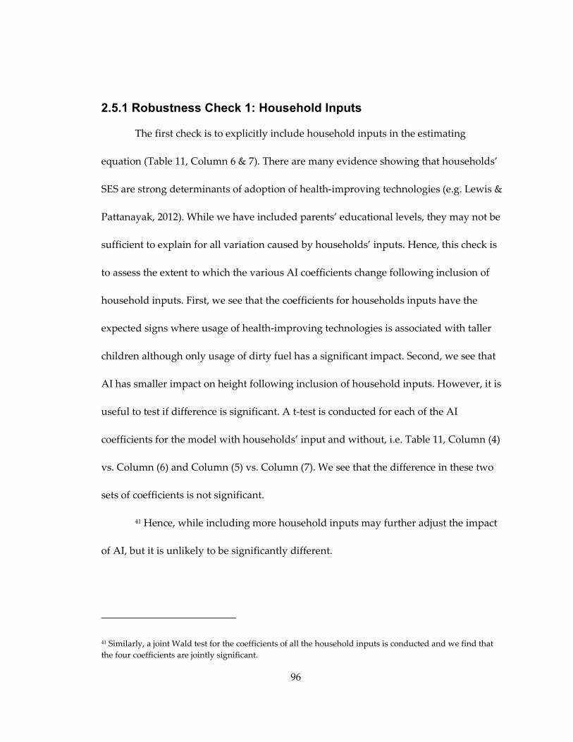
96
2.5.1 Robustness Check 1: Household Inputs
The first check is to explicitly include household inputs in the estimating
equation (Table 11, Column 6 & 7). There are many evidence showing that households’
SES are strong determinants of adoption of health-improving technologies (e.g. Lewis &
Pattanayak, 2012). While we have included parents’ educational levels, they may not be
sufficient to explain for all variation caused by households’ inputs. Hence, this check is
to assess the extent to which the various AI coefficients change following inclusion of
household inputs. First, we see that the coefficients for households inputs have the
expected signs where usage of health-improving technologies is associated with taller
children although only usage of dirty fuel has a significant impact. Second, we see that
AI has smaller impact on height following inclusion of household inputs. However, it is
useful to test if difference is significant. A t-test is conducted for each of the AI
coefficients for the model with households’ input and without, i.e. Table 11, Column (4)
vs. Column (6) and Column (5) vs. Column (7). We see that the difference in these two
sets of coefficients is not significant.
41 Hence, while including more household inputs may further adjust the impact
of AI, but it is unlikely to be significantly different.
41 Similarly, a joint Wald test for the coefficients of all the household inputs is conducted and we find that the four coefficients are jointly significant.

97
2.5.2 Robustness Check 2: ‘Placebo’ test: older and younger children
Next, we conduct two placebo tests. We see how the AI exposure in 1997
influenced children born a year later 1998. The rationale is that these children should not
be affected by air pollution which happened before they were born, but if they are, this
means that AI is correlated with other spatial characteristics that drive outcomes. We
conduct this test for all outcomes using specification (4) and (5) from Table 11.42 The
results are obvious as the AI coefficient is not significant in the majority of cases (Table
14).
We repeat this test for the cohort born one year before. From the main outcomes
studied so far, we expect the impacts of air pollution to be smaller, if at all there is any
impact. This is because we see that no outcomes were affected by exposure in the first
six months of life. Hence, if we were to see a large impact, this could again signify that
spatial correlation is affecting the results. As expected, most of the AI coefficients are not
significant (Table 15).
42 We cannot include lung capacity because younger children were not required to take the spirometry test in the IFLS.

98
Table 14: Regression results for all outcomes for the cohort born one year after the cohort in the main sample
(1) (2) (3) (4) (5) (6) HAZ
(t+1) cohort HAZ
(t+1) cohort Cognitive test
(t+1) cohort Cognitive test
(t+1) cohort WAZ
(t+1) cohort WAZ
(t+1) cohort VARIABLES
AI -0.565 -0.165 -3.825 AI at first trimester -1.454 -0.097 -1.721 AI at second trimester 3.356 0.325 -1.193 AI at third trimester 4.163 0.928 4.009 AI at fourth trimester -3.203 -0.314 -3.465 AI at fifth trimester 3.277 0.158 -1.594 Male -0.007 -0.007 Age (months) 0.003* 0.004 Father at least high school 0.202** 0.213** 0.002 0.005 0.230* 0.254** Mother at least high school 0.033 0.017 0.037* 0.036* -0.156 -0.175 Precipitation 0.001 0.002 -0.001 -0.000 -0.006 -0.001 Temperature 0.373 0.258 -0.039 -0.059 -0.869 -0.964 Father’s height 0.010** 0.010** Mother’s height 0.019*** 0.018*** Father’s weight 0.023*** 0.023*** Mother’s weight 0.023*** 0.022*** Constant -6.844*** -7.264*** 0.212 -0.033 -4.709*** -5.542***
Observations 700 700 778 778 698 698 R-squared 0.088 0.102 0.040 0.046 0.126 0.129 Standard errors clustered at district level (not shown) *** p<0.01, ** p<0.05, * p<0.1

99
Table 15: Regression results for all outcomes for the cohort born one year before the cohort in the main sample
(1) (2) (3) (4) (5) (6)
HAZ (t-1) cohort
HAZ (t-1) cohort
Cognitive test (t-1) cohort
Cognitive test (t-1) cohort
WAZ (t-1) cohort
WAZ (t-1) cohort
VARIABLES
AI -0.014
0.251
2.383 AI at first trimester
1.048
0.504*
1.146 AI at second trimester
-1.048
0.430
0.350 AI at third trimester
2.028
0.529
2.314 AI at fourth trimester
3.049
0.268
4.958* AI at fifth trimester
0.215
0.263
-0.386 Male
-0.015 -0.016 Age (months)
0.001 0.003 Father at least high school 0.090 0.094 0.030* 0.030* 0.003 0.014
Mother at least high school 0.506*** 0.491*** 0.032 0.030 0.226 0.212 Precipitation 0.014 0.014 -0.000 -0.001 0.006 0.005 Temperature 0.620 0.520 0.310** 0.320** -0.191 -0.174 Father’s height 0.010** 0.010**
Mother’s height 0.005 0.005 Father’s weight
0.025*** 0.024*** Mother’s weight
0.024*** 0.023*** Constant -2.989** -3.314*** 0.658** 0.358 -3.773*** -3.656***
Observations 714 714 758 758 718 718 R-squared 0.080 0.084 0.047 0.051 0.135 0.141 Standard errors clustered at district level (not shown) *** p<0.01, ** p<0.05, * p<0.1

100
2.6 Discussions and Conclusions
There is little or no evidence on potentially significant long-term impacts of
early-life exposure to environmental pollution, especially so in developing countries
(Currie and Vogl, 2012). This knowledge gap is especially poignant now as air pollution
has increased to unprecedented levels in many Asian cities. Our findings that exposed
children are shorter, perform worse in cognitive tests, and have lower lung capacity
adds to the thin empirical evidence base. Of these, the height outcome arguably matters
most due to the strong evidence showing correlation between height and socioeconomic
outcomes in developing countries. Results on height are also strengthened as we
repeated the analysis using the 2000 IFLS. We find that exposed children already
showed signs of being shorter compared their unexposed or less-exposed peers at
around 2-3 years old and the height differential persisted and in fact, strengthened 7
years later.
We also find tentative results showing that first trimester exposure matters most
for height and cognitive test outcomes, while second and third trimester exposure
matters most for lung capacity. These trimesters results while interesting, are difficult to
interpret as there are no medical hypotheses so far to confirm or refute if any particular
stage of fetal development is most sensitive towards air pollution. However, a consistent
finding throughout the analysis and robustness check is that postnatal exposure are not
associated with negative outcomes. Of the related studies, only Morales et al. (2015)

101
looked at postnatal exposure and they also did not find negative impacts from postnatal
exposure. However, it is unclear if the lack of negative impacts from postnatal exposure
is due to either biological reasons or that it is easier to protect the infant from poor air
quality. This is an important and interesting question that should be investigated in
depth.
Lastly, our findings also suggest the lack of catch-up growth which is a grim
prospect if it is in fact true. A possible hypothesis is that the magnitude of the shock
matters in determining catch-up growth. Cameron et al. (2005) showed using different
samples that children with very low HAZ fail to exhibit catch-up growth whereas those
with slightly higher (but still negative) HAZ do exhibit catch-up growth. This is also
evident in the empirical strategy of studies that found evidence of catch-up growth such
as Adair (1999), Tiwari et al. (2013), and Rabassa et al. (2012). These studies did not use a
single event shock and instead employed the ‘deviation from mean’ strategy which thus
included smaller ‘shocks’. This means that smaller deviations which are still registered
as ‘shocks’ have minimal impact on health and thus would not register in the long-run.
In comparison, most other studies that found no evidence of catch-up growth exploit a
single catastrophic event as the identification strategy. One way to probe this issue is to
use future rounds of IFLS to examine if these impacts persist and if additional outcomes
such as labor capital and educational attainment would be affected as well.

102
Up till now, air quality management programs mostly highlight
contemporaneous health burden. However this study demonstrates that they are
possibly sizable costs to air pollution which are hitherto unconsidered. As air quality is
traded off by increasing economic activities in many places, perhaps planners are
displaying short-termism that will impose large penalties on future generations which
are impossible to reverse.

103
3. Preference heterogeneity and adoption of environmental health improvements: Evidence from a cookstove promotion experiment
3.1 Introduction
Many development projects aim to encourage households’ adoption and usage
of new technologies that improve health and socioeconomic outcomes (Besley & Case,
1993). However, these interventions are often faced with resistance as participants are
slow to adopt and/or use the technologies (Jack et al., 2015). As this is a commonly
observed problem across many areas such as agriculture, water and sanitation,
household energy, mosquito bednets, and others, numerous experiments have been
conducted to search for strategies to improve uptake and drive demand for these
technologies (Ashraf et al., 2010; 2013; Cohen & Dupas, 2010; Berry et al., 2012; Tarrozi et
al., 2013; Dupas 2014; Fischer et al., 2014). These experiments generally attempt to
reduce costs of uptake or increase knowledge on the benefits of uptake (Pattanayak &
Pfaff, (2009) provide a theoretical model to explain adoption). While some inroads have
been made to understand drivers of demand, there are still many questions that need to
be answered. In particular, many interventions treat participants as if they have
homogenous preferences and offer only one version of the technology. While low
preference variability may be true for technologies with basic or limited attributes such
as vaccination or nutritional supplement, demand heterogeneity may be more common
for complex technologies such as improved water and sanitation facilities (Jenkins &

104
Curtis, 2005; Casabonne & Kenny, 2012). More importantly, failure to take
heterogeneous cost and benefit into consideration may generate inaccurate conclusions
regarding outcomes of the interventions (Whittington et al., 2012).
In this study, we combine responses from a discrete choice experiment (“DCE”)
and actual purchases following a randomized stoves promotion campaign to provide
evidence of heterogeneous demand for improved cookstoves (“ICS”) in Uttarakhand,
India. Our findings show that it is possible to characterize preferences for various stoves’
attributes using a simple discrete choice experiment and verified by ensuing stoves
purchases. Furthermore, we also show that households would willingly purchase ICS if
attributes of the marketed stove are aligned with their preferences. Lastly, we also show
that usage of the newly-purchased stoves is not correlated with purchase preferences.
These findings could potentially improve the effectiveness of future ICS interventions.
To understand preferences, we apply generalized multinomial logit methods to
analyze DCE data collected during baseline surveys among all sample households in
Uttarakhand, India (Magidson & Vermunt, 2004). In the DCE, respondents completed a
series of choice tasks in which they considered differences – in terms of price, number of
cooking surfaces, amount of smoke emissions, and fuel requirements – between
biomass-burning ICS and traditional stoves. In the context of studying demand for ICS,
for which well-developed markets do not currently exist, a particular advantage of DCE
preference elicitation is to allow consumers to explicitly consider tradeoffs between

105
hypothetical stove alternatives with varying levels of these types of attributes (Louviere
et al., 2000; McFadden & Train, 2000).
We then consider whether households with specific types of preferences, as
categorized through latent class analysis (“LCA”) of DCE choices, are more or less likely
to purchase an ICS during a randomized ICS promotion campaign. A follow-up survey
conducted several months after the intervention sheds additional light on use of the
intervention ICS. We find that about half (52%) of sample households can be categorized
as initially ‘uninterested’ (we call these class 3) in the positive attributes of ICS. These
households have lower wealth, are older, and are less aware of the health damages
caused by smoke inhalation at baseline. The other two classes are primarily
distinguished by their relative responses to smoke emissions reductions versus reduced
fuel requirements and increased convenience, with class 1 (27%) being mainly interested
in smoke emissions reductions, and class 2 (20%) having much higher relative demand
for the full set of ICS attributes. Consequently, we observe that class 3 households were
significantly less likely to purchase any ICS during the first of three visits by the sales
teams implementing the randomized sales campaign. However, a promising
development is that they became more receptive towards the stoves in subsequent visits.
Among the other two groups, class 1 was more likely to adopt an electric, rather than a
biomass-burning ICS, suggesting that distaste for smoke may play a particular role in
motivating purchase of the electric stove. We also find some evidence that class 2

106
households respond more strongly to randomized rebates when considering the
purchase of the cleaner-burning biomass ICS. Importantly, perhaps because the stove
promotion campaign was designed to address commonly-identified barriers to adoption
of environmental health technologies such as information and liquidity constraints
(Bensch et al., 2014), very few observable household or community-level covariates
explain stove purchases following the promotion campaign. Lastly, we also find that
households’ subsequent usage of their newly purchased stoves is not correlated to their
preference classes. This suggests that there are different preference mechanisms
governing purchases and usage.
This paper makes several contributions. First, we add to a thin literature on
private demand for ICS by examining how households respond to an ICS sales offer that
offers a choice between two very different technologies – an improved biomass-burning
stove and an electric coil stove. Existing ICS intervention studies largely ignore user
preferences and focus on the demand for a single pre-selected technology with a specific
set of features, or seek to isolate differences in demand by varying technologies across
the arms of an experiment rather than allowing users to choose the technologies they
prefer from several options (Mobarak et al., 2012). Second, we seek to better understand
the variation in preferences and tastes for different ICS options, by conducting latent
class analyses of stated DCE data. Third, after systematically characterizing the choice
patterns revealed in the DCE data, we investigate the extent to which preference type is

107
related to the choices revealed in the randomized ICS promotion campaign, which
speaks to long-standing questions about the reliability of subjective and stated
preference data (Bertrand & Mullainathan, 2001; Borghans et al., 2008; Carson et al.,
1996). Finally, we generate new evidence on the interaction between preferences, prior
exposure to promoting micro-institutions, and intervention outcomes. These
contributions collectively serve to elucidate important supply- and demand-side
features of the market for ICS. Understanding of these features is critical for developing
policies that encourage product development and market segmentation, both of which
seems essential for stimulating wider diffusion of these and other similar quasi-public
goods.
3.2 Background and Motivation
The use of solid biomass or coal fuels for basic household cooking and heating
remains widespread throughout the world, and represents approximately 15% of global
energy use (Smith et al., 2000; Legros et al., 2009). Such fuels are often burned in
inexpensive and inefficient stoves, which results in damages to health from respiratory
illnesses and other conditions (Ezzati & Kammen, 2001; Bruce et al., 2006; Martin et al.,
2011), to local environments and development due to unsustainable and time-intensive
harvesting of biomass, and to the global climate system as a result of emission of black
carbon particles and ozone precursor gases (Bond et al., 2004; Ramanathan &
Carmichael, 2008). These negative effects of traditional stoves have prompted great

108
interest in, and a new push towards development and dissemination of more efficient
and cleaner-burning improved cook stoves such as gas-, electric-, or cleaner biomass-
burning technologies (GACC, 2010).
43
Yet despite the very significant problems associated with traditional stoves,
adoption of cleaner burning stoves has been slow. New biomass-burning technologies
have not reached scale, and other alternatives – mainly electric and gas stoves – have
been constrained by the lack of a robust distribution system for the energy sources and
fuels on which they depend. Perhaps nowhere is the scale of this challenge greater than
in India, the largest potential market for such technologies and one of the world’s hot
spots for biomass burning in inefficient stoves. Progress in India has been particularly
slow with only several tens of thousands of more efficient biomass stoves sold in each of
2011 and 2012, even though globally sales were in the millions (GACC, 2012; Colvin et
al., 2013). Beyond well-known problems of high costs and a weak supply chain,
researchers and practitioners have claimed, with only limited evidence from rigorous
field studies, that the existing range of biomass ICS prototypes are unreliable and not
sufficiently adapted to local cooking requirements and user preferences (Duflo et al.,
2008; GACC, 2011; Jeuland & Pattanayak, 2012; Lewis & Pattanayak, 2012; Singh &
43 We use the term improved cook stoves (ICS) in this paper to refer to both of these types of technologies, e.g., more efficient biomass stoves, as well as stoves that use advanced, cleaner-burning fuels such as LPG or electricity.
109
Pathy, 2012; Shell Foundation, 2013). Meanwhile, more widely accepted ICS
technologies such as LPG and electric stoves remain costly for poor households, and the
fuels lack a robust and strong supply chain or distribution system in many rural areas
(Lewis et al., 2014). Thus, a range of recent studies conducted in South Asia suggest that
major challenges remain in the push to promote ICS, with regards both to private
demand for these new technologies (Mobarak et al., 2012), and to the realization of
health and other welfare benefits from their use (Hanna et al., 2012).
These recent negative findings raise important questions about ICS promotion
and dissemination, but they stand in sharp contrast to those from other field studies,
mainly conducted in East and West Africa, that suggest that ICS promotion can in fact
succeed, at least in the short-term (Levine et al., 2013; Bensch & Peters 2014). Indeed, the
range of recent findings on ICS highlights several points that have previously been
emphasized in the broader literature on demand for environmental health
improvements. First, the demand for such health improvements is often low, and is
related to consumers’ diverse preferences, circumstances and income constraints
(Pattanayak & Pfaff, 2009). Second, household decision about whether or not to adopt
and continue to use ICS is obviously dependent on their knowledge of the associated
costs and benefits (Liu, 2013; Tarozzi et al., 2014). Successful promotion strategies for ICS
and other environmental health technologies have worked to address some of these
barriers, by engaging with institutions that are able to effectively implement social

110
mobilization campaigns (Pattanayak et al., 2009), or by providing financing options and
reducing the risk of adoption (Levine et al., 2013).
In all, prior work on promoting demand for ICS typically focus on reducing cost
of adoption or increasing knowledge on the benefits of adoption. Rather, a central goal
of this study is to characterize the variation in deep-lying preferences for ICS. This latent
heterogeneity has important implications for policy design (Heckman, 2001) but is an
under-researched topic in economics (Ravallion, 2012), especially as it pertains to
improving adoption of environmental health technologies and other similar quasi-public
goods. However, latent heterogeneity in preferences is not easily observed or measured.
The most direct way to elicit measures of heterogeneity is to ask respondents directly
using stated preference methods. For example, Cardenas et al. (2013) used a series of
question to assert respondents’ level of trust and pro-sociality. Such method of obtaining
information from respondents has generated a healthy dose of skepticism from some
economists. Bertrand and Mullainathan (2001) argued that subjective data are unsuitable
as dependent variables because of correlated measurement errors. However, rather than
a blanket disapproval from all, Manski (2000) and McFadden (2013) supported the usage
of subjective data if the data is obtained from binary-type question and questions posed
to respondent are simple and familiar. Indeed, there are more recent studies that test the
boundary of the usefulness of subjective data. The aforementioned Cardenas et al. (2013)
and Johansson-Stenman et al. (2013) both used this method to measure how stated trust

111
attitudes correlate with actual behaviors. Liu & Huang (2013) used subjective risk
preferences to predict adoption of new agricultural technology.
3.3 Modeling
Following Pattanayak and Pfaff (2009), the household’s decision to adopt an ICS
or any technology is governed by its utility function and various constraints (health
production, time, and budget). The decision essentially boils down to a comparison of
marginal benefits against marginal costs at the household level:
(17)
where the LHS is the marginal benefit of adopting technology (a) for household
type i. Accordingly, adoption of the technology provides intrinsic utility and health
benefits (s). These are benefits are monetized by the marginal utility of income, . On
the other side of the ledger are the marginal costs. Assuming a discrete good, the costs
are simply the price of purchasing a and the cost of obtaining knowledge (k) about a. In
practice, most studies attempt to trigger adoption decisions by randomizing price of the
technology, cost of acquiring knowledge of its benefits, and/or ease of usage, i.e., making
changes to the RHS. Parameters on the LHS are generally neglected and we can see that
this marginal condition may differ for different types of household, i.e. the type j’s and
k’s households may only adopt the technology at a different price compare to type i.
More importantly, we will not be able to directly characterize the heterogeneity in

112
preferences even through randomizing the RHS variables. As such, we begin by first
using a DCE to sort respondents into different preference parameters or groups.
3.3.1 Modeling heterogeneous preferences for ICS
The framework for analyzing the DCE data used in this study is based in random
utility theory. We model the repeated household choices from among different
combinations of stove alternatives that vary according to well-defined levels of four
attributes: price, fuel requirement, smoke emissions, and the number of cooking
surfaces. The random utility model we apply assumes that the indirect utility associated
with a particular alternative can be written as a function of its attributes, and household
characteristics:
(18)
where:
= the utility of household i associated with cooking alternative j in a choice
set, where t indexes the number of choice tasks completed (4 per household);
= the non-stochastic portion of the utility function for household i;
= the price of cooking alternative j in task t;
= a parameter which represents the marginal utility of money for household i;

113
= a vector of non-price attribute levels for cooking alternative j in task t;
= a vector of parameters which represent the marginal utility for household i
associated with the different non-price attributes of the alternatives;
= a vector of characteristics for household i; and
= a stochastic disturbance term.
Assuming that households maximize utility within a given choice task, they will
select alternative j from among the set of K alternatives presented to them if and only if
alternative j provides a higher overall level of utility than all the other alternatives, i.e. if
> for all j in set K, where j ≠ k, such that . Assuming a linear
specification of utility and a Type 1 extreme-value error
distribution for the disturbance term, the probability that alternative j will be selected
from choice set t corresponds to the standard conditional logit model (McFadden, 1981).
The conditional logit model is estimated using maximum likelihood; the values of the
coefficient values and are selected to maximize the likelihood that one would
observe the choices actually observed in a given sample of respondents.
In this paper, we relax the restrictive assumption of the conditional logit that
requires a single set of fixed β coefficients, and instead estimate two types of mixed (or

114
random parameters) logit models.44 The first is the mixed logit, which allows for
unobserved heterogeneity in tastes across individuals, as specified through inclusion of
respondent-specific stochastic components for each of the estimated coefficients β in
the model. In the mixed logit model, the choice probability function is described by the
integral of the product of conditional individual probabilities over all choice occasions t,
where the marginal utilities for different attributes are measured by :
(19)
where and denotes the density of the individual
disturbance terms given the fixed parameters Ω of the distribution. The stochastic
portion of utility then flexibly accommodates correlations both across alternatives and
choice tasks. The coefficients are estimated using simulated maximum likelihood
(Revelt & Train, 1998). The ratios of coefficients derived from the model then yield the
marginal utility to individual i for an additional unit of a particular attribute, in money
terms.
44 There are several problems with the conditional logit, including violation of the independence of irrelevant alternatives (IIA) assumption, the inability to account for correlation across a respondent’s choices, and the lack of consideration of differences in individual tastes other than those related to the specified attributes of alternatives.

115
The second is the latent class logit, a discrete version of the mixed logit, which
allows us to categorize households into distinct groups based on the similarity of their
choice patterns. In these models, maximum likelihood methods are used to identify S
class types (where S is an integer selected by the modeler) with similar weighting of
various attributes of the choice alternatives.45 The probability of observing respondent i
selecting alternatives j over T choice tasks is written as a product of the probability the
respondent belonging to class s and the probability that the sequence of alternatives is
chosen:
(20)
The first term in equation (20) is the unconditional probability of class
membership, while the second term corresponds to the probability of choosing a
sequence of alternatives based on their attributes. In most applications of the latent class
approach, the vector in the first term includes characteristics such as age, education
level, and income. In this paper, however, we omit these characteristics and replace
with a vector of individual-specific constants because our goal is to use only information
revealed by the choices households make in the DCE to predict adoption of clean
45 See Error! Reference source not found. for a more detailed treatment of latent class logit models.

116
stoves.46 This modeling approach is also conservative as it relies on fewer assumptions
to estimate stated preferences. In the second term, the taste parameters are
subscripted with the class indicator s, meaning that every respondent in class s has
identical tastes for the attributes of the choice alternatives in the DCE.
Rather than assuming a specific number of classes, we rely on the Bayesian
Information Criterion (BIC) to select the best-fitting model with up to 10 different classes
(Roeder et al., 1999). We then assign a household to the particular class for which its
probability of membership is greatest, and study the correlates of class membership
using a multinomial logit model.
3.3.2 Modeling the adoption decision
From the stove promotion campaign and follow-up surveys conducted several
months after the promotion campaign, we observe households’ ICS purchase and use
decisions. We regress these outcomes on latent class membership as identified based on
the responses in the DCE. The most general model we estimate can be written as:
(21)
46 If socioeconomic characteristics were also included in the estimation of class membership probabilities, these predicted probabilities would then partially reflect these observable factors. In turn, this would conflate our investigation of latent preference heterogeneity which are driven by both observed and unobserved characteristics.

117
In this model, is a dummy variable representing purchase of an intervention
ICS by household i in community j. More specifically, we analyze purchase of an ICS
during the initial sales visit and during the entire campaign. The variable is a
dummy variable that is equal to 1 if the household i has preferences of type k and 0
otherwise (as revealed by the LCA)47; represents a rebate amount randomized at the
household-level in the communities exposed to the stove offer; is a vector of l
household and community variables that influence the purchasing decision; is an
error term clustered at the community level; and is the usual individual idiosyncratic
error term. The coefficients are estimated using OLS regression, and allow us to
consider the effects of preferences and price incentives, ( and , respectively) on
outcomes, and whether these preference effects vary across institutional strata ( ).
In the ICS purchase models, we first group the improved biomass and electric
stoves into one general category and analyze adoption of any ICS, using a linear
47 To test for sensitivity of our results to the definitions of class membership, we also estimated the same models using the continuous probabilities of class membership generated by the latent class logit procedure. These results are qualitatively identical to those presented in the paper, and are available upon request.

118
probability model. We consider more parsimonious specifications for equation 3 as well
as the complete model. We then apply a multinomial logit model that treats the three
options as a categorical outcome for each household (no stove, electric, or improved
biomass stove). Standard errors in all analyses are clustered at the community or hamlet
level as this is the administrative level at which the stove promotion campaign was
assigned.
3.4 Research Site and Data
The target region for this study, in the Northern Indian state of Uttarakhand, is a
particularly relevant location for a study of the demand for ICS, due to the confluence of
several factors: a) growing national and local-level interest and activity in the
dissemination of more efficient household energy products; b) increasing awareness and
demand for more efficient cooking technologies, due to the rising costs of fuels (as a
result of growing scarcity of firewood and concerns over the environmental impacts of
deforestation) and greater concern over the health effects of indoor air pollution; and c)
location in a region (the Hindu Kush-Himalaya) that is particularly vulnerable to the
impacts of climate change. Baseline surveys were conducted in August – October 2012;
the promotion intervention occurred from August – November 2013, with follow-up
surveys occurring shortly thereafter in November and December 2013.

119
3.4.1 Sampling Frame
The sampling frame for the study consists of 97 geographically distinct
communities (or hamlets) located in 38 Gram Panchayats (GPs) in the Bageshwar and
Nainital districts of Uttarakhand (Figure 9).
Within each of the 38 GPs, we randomly selected households according to the
size of the GP. In small GPs, a minimum of 20 surveys were collected; in medium ones
30; and in large ones 40. If a GP was divided by distinct landmarks (e.g., half the village
was to the north of the main road, half the village was to the south), the target number of
surveys was split equally among these groups. Upon arrival in the village, the
population of the GP was divided by the target number of surveys and every nth
household (no more than every 8th house) was surveyed until the target number of
surveys was reached. This strategy ensured that surveys were collected throughout the
entire extent of the GP and created variation in the number of hamlets sampled in each
GP. The “official” number of distinct hamlets sampled in this way was 106; some of the
smallest of these were later combined with nearby hamlets for the purpose of the ICS
promotion intervention to yield the final set of 97 hamlets.
Efforts were made to interview each sampled household. If a randomly-selected
household was unavailable during the entire day of baseline fieldwork in a particular
hamlet, or if it did not have an eligible respondent (i.e., the primary cook and/or head of
the household were unavailable) or refused to participate, neighboring houses were

120
randomly selected as replacements.48 Field supervisors performed household
introductions, recorded GPS coordinates and elevation data, and oversaw quality
control checks in each village. The final sample for the household survey consisted of
1,063 households.
3.4.2 Baseline surveys and the DCE
The questionnaires used in the baseline surveys included both household and
community instruments (completed by a village leader or key informant). Respondents
(both the male and female head of household or primary cook) answered questions on
environmental and stove-related perceptions, household socio-demographics, stove and
fuel use, socio-economic characteristics, risk and time preferences, and completed the
DCE. Whenever possible, women answered questions related to socio-demographics,
stove and fuel use, whereas men completed the DCE, socio-economic, and time and risk
preference sections. Environmental and stove-related perceptions questions were
randomized ahead of time to the male or female head of the household / primary cook,
subject to his/her availability (which was recorded on the survey form). If one of these
two was unavailable for the survey (most often the male), the other eligible respondent
completed all questionnaire sections. In addition, a sub-sample of households
participated in a 24-hour biomass fuel weighing exercise for monitoring of fuel
48In total, 118 households were replaced in this way. Thirty-three households refused to participate, while an additional 85 could not be interviewed because they were not present during the day of the fieldwork.

121
consumption. The survey instruments were pre-tested prior to the initiation of fieldwork
in approximately 200 households located in 9 villages in northern India.
Figure 9: Study Design

122
The attributes included in the stove decision exercise, described above, and their
levels, were selected following a series of eleven focus groups conducted with over 100
respondents in villages similar to sample villages. Attributes eliminated due to lack of
clarity or salience to respondents included time savings (fuel savings were deemed
easier to understand by respondents), operation and maintenance requirement, fuel
loading approach, lifespan of the stove, and type of fuel allowed. We used SAS software
to select efficient combinations of attribute levels for measuring main effects. An
example of a choice task, and important features of the design are summarized in Figure
10 and Table 16.
Figure 10: An example choice task in the stove decision exercise

123
Table 16: Summary of discrete choice experiment design
Attributes Levels Traditional stove
level
Price (Rs.)1 500 1000 2500
0
Fuel requirement 1 3 4
3
Smoke emissions Low High
Highest Highest
Number of cooking surfaces
1 2
1
Importantly, given the fact that the randomized intervention allowed for a choice
between an electric and biomass-burning ICS, the improved options presented in the
DCE were biomass-burning stoves. At the start of the stove decision exercise, this ICS
stove alternative was described to respondents in detail, and each of the attributes was
explained by the enumerator using a specific script accompanied by pictures. At the end
of this description, all respondents completed a 4 question comprehension test. If a
respondent answered any questions incorrectly, the relevant description was repeated
and the enumerator again verified comprehension before proceeding. Next the
respondent was reminded of his/her budget constraint, was told that the ICS options
would last 3 to 5 years and cost roughly 250 Rs. per year to maintain, was assured that
there were no right and wrong answers, and was reminded that the exercise was purely

124
hypothetical. In each of four choice tasks completed during the survey, respondents
were asked to select their preferred option from a set of two ICS alternatives or their
existing stove (i.e. neither of the presented ICS). If they selected one of the ICS
alternatives, respondents were asked to confirm their willingness to pay the price listed
on the card: “If you had the possibility to purchase this stove at the price stated, would
you be willing to make that purchase, if the payment was required at the time of
purchase?”49 This confirmation was included to decrease the potential for hypothetical
bias in the stated preference responses (Murphy et al., 2005). Following each choice task,
debriefing questions were asked to probe the decision-making process and assess the
certainty of respondent answers.
3.4.3 The intervention
The ICS promotion intervention was implemented and therefore randomized at
the hamlet level; all sample households living in treatment communities were visited by
sales teams working for a local NGO; households living in control communities were not
(Figure 9: Study Design). Following careful field piloting of potential ICS promotion
techniques (Lewis et al., 2013), trained ICS sales people, working in teams of 2, visited
treatment households and conducted intensive promotion activities with them. First, these
49 Prior to this question, all respondents were reminded to consider their household budget carefully when choosing their preferred options. The specific text in the questionnaire was: “There are no wrong or right answers to these questions. When you make your choice, keep in mind your household budget and your other financial constraints. You should consider carefully whether the benefits of an improved stove would be worth paying for their cost, in terms of stove cost and maintenance requirement. Remember that the improved stoves last 3 to 5 years and cost about 250 Rs. per year to maintain.”

125
teams presented treatment households with an information sheet and explanation of ICS
features, even as they performed a live tea-making demonstration comparing the two
different stoves being offered: an electric coil and biomass-burning ICS.50 The
information sheet (see Appendix G) and demonstration were designed to inform
households about the benefits (reduced smoke, firewood savings, time savings) and costs
(price, electricity cost and risk of electric shocks) of these stoves. Then, once the
demonstration was complete, the sales people explained the ICS payment plan to
households. Specifically, all households were given the choice of paying for the stoves
upfront or in three equal installments (including a modest financing fee of 60 or 80 Rs.,
depending on the stove) that would be collected over a period of 4 weeks (i.e., in 3
installments collected 2 weeks apart). Roughly two thirds of purchasing households opted
to pay for the ICS in installments.
In addition, households were told that they would receive a randomized rebate to
be given at the time of the final payment if they were found to be using the stoves (as
observed during unannounced visits). Those paying for stoves upfront were also eligible
for the rebate and thus were also revisited roughly one month later. Prior to the
households indicating whether they would purchase the ICS, this randomized rebate was
revealed by drawing a chit out of a bag. The bag contained equal numbers of chits
corresponding to the three potential rebate levels, low – 25 Rs. (a 2.5% discount),
50 We offered two types of biomass ICS in the initial piloting activities, but it quickly became apparent that demand for these technologies was low. After observing great interest in a similarly-priced electric stove in later pilots, we decided to offer it alongside the more affordable of the biomass-burning stoves.

126
medium – 200 Rs (a 20% discount), and high – equivalent to a full installment (a 33%
discount). The electric stoves were sold to households for 900 Rs. (or 960 Rs. for those
paying in installments); biomass stoves were 1300 Rs. (or 1,380 Rs. with installments);
these prices corresponded to the stove-specific prices paid to suppliers. As such, the
amount of the high rebate (320 or 460 Rs.) varied somewhat based on the stove that was
chosen by a household. Due to concerns over the endogeneity of the high rebate amount,
we replace this varying amount with 320 Rs. in our analyses (the rebate for the electric
stove); none of our results are sensitive to this approach.51 Finally, because of this design
and the two follow-up visits to intervention communities that it entailed, households that
initially declined the ICS during the first visit were allowed to purchase a stove during
follow-up visits so long as they caught up with the installment payments they had missed.
We opted for this intervention design based on both small-scale piloting
experiences in 8 villages and on our analyses of responses in the DCE, which showed
great heterogeneity in overall demand, as well as relative weighting that households gave
to smoke reductions (greatest with the electric stove) vs. fuel savings (Bhojvaid et al.,
2013; Jeuland et al., 2013). This evidence on heterogeneous preferences made us think
that artificially constraining the choice set by randomizing specific stoves to different
intervention communities might depress demand, though the tradeoff is that it prevents us
from clearly differentiating the impacts of stove adoption by ICS type. On the basis of
power calculations and our estimation of the differential treatment effects expected from
51 The sensitivity of purchases to the rebate level that we estimate may thus be somewhat overestimated, particularly for the biomass stove.

127
the alternative rebate levels, 71 of the baseline hamlets (corresponding to 771 of the 1063
baseline households) were randomly assigned to the treatment group.52 The remaining 26
hamlets were control hamlets that did not receive any visits from the stove promotion
teams (Figure 9).
3.4.4 Sample balance and descriptive statistics
This paper reports on data collected at two points in time; at baseline surveys
and post-intervention. The intervention data include only basic information on whether
a household purchased a stove, which ICS it chose, the randomly-assigned rebate level,
and the specific payment made during each visit from the sales team. Thus, we analyze
the DCE data that pertain to the entire sample of households that includes treatment and
control communities, but only differentiate adoption results by class for households in
the treatment communities.
Descriptive statistics from the baseline sample of 1,063 households are
summarized in Table 17: Baseline descriptive statistics. In 73% of surveys, the
respondent for all questions was a woman (primary cook and/or female head of
household). Interviews with the remaining 27% generally included both a male head of
household and the primary cook, according to the assignments described above. The
average household size at the time of the survey was 4.8 people. Overall, 73% of
52 Nine of these 771 treatment households could not be re-located during the stove promotion campaign, and therefore do not appear in any of the results.

128
households are in the open/general caste category, and 25% are scheduled caste or tribe.
Sample households are generally rural, poor, and primarily agricultural. Over half of the
survey population reported being below the poverty line, and access to credit was low
(with just 15% of households availing of credit in the prior year). Almost all have
electricity, but only 24% report having electricity all the time. Just over 7% of household
members were reported to have experienced a cough or a cold in the two weeks prior to
the survey.
At the time of the interviews, nearly all households had a traditional mud stove
(40%) or traditional 3-stone stove (49%). Other commonly-found stoves were LPG (29%),
or a traditional metal sagarh stove (21%). Very few households had kerosene pump
stoves (1.2%) or biogas stoves (1%). The average number of stoves owned by each
household was 1.4. Nearly all (93-98%) households owning LPG and traditional stoves
reported using these in the week prior to the survey, and almost all LPG-owning
households used it alongside a biomass stove (only 7% of these did not also use their
traditional stoves on a daily basis). Households reported total stove use time to be 5.7
hours/day, and identified that the three best aspects of traditional stoves were: the taste
of the food (90%), the cost of the stove (55%), and the ability to cook all foods (7%). The
four worst features identified were the smoke that is produced (63%), the cleaning
requirements (45%), and the amount of fuel required and the heat given off by the stove
(22%).
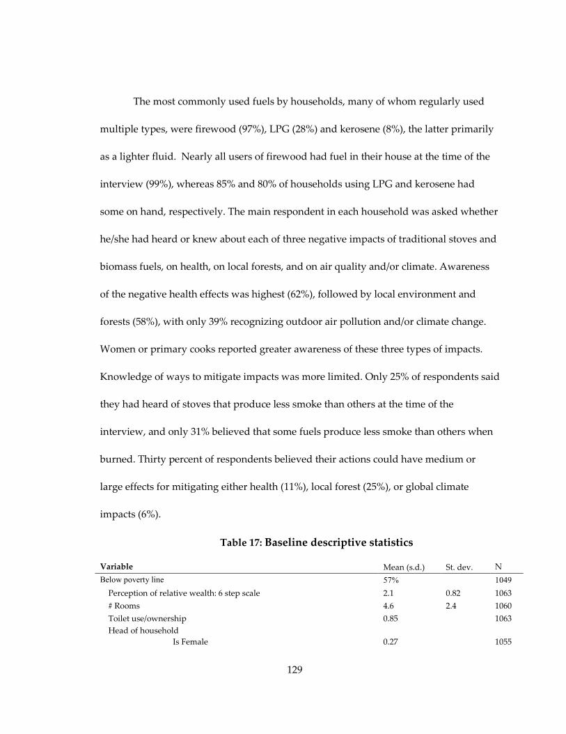
129
The most commonly used fuels by households, many of whom regularly used
multiple types, were firewood (97%), LPG (28%) and kerosene (8%), the latter primarily
as a lighter fluid. Nearly all users of firewood had fuel in their house at the time of the
interview (99%), whereas 85% and 80% of households using LPG and kerosene had
some on hand, respectively. The main respondent in each household was asked whether
he/she had heard or knew about each of three negative impacts of traditional stoves and
biomass fuels, on health, on local forests, and on air quality and/or climate. Awareness
of the negative health effects was highest (62%), followed by local environment and
forests (58%), with only 39% recognizing outdoor air pollution and/or climate change.
Women or primary cooks reported greater awareness of these three types of impacts.
Knowledge of ways to mitigate impacts was more limited. Only 25% of respondents said
they had heard of stoves that produce less smoke than others at the time of the
interview, and only 31% believed that some fuels produce less smoke than others when
burned. Thirty percent of respondents believed their actions could have medium or
large effects for mitigating either health (11%), local forest (25%), or global climate
impacts (6%).
Table 17: Baseline descriptive statistics
Variable Mean (s.d.) St. dev. N
Below poverty line
57% 1049
Perception of relative wealth: 6 step scale 2.1 0.82 1063
# Rooms 4.6 2.4 1060
Toilet use/ownership 0.85 1063 Head of household Is Female
0.27
1055

130
Age (years) Education (years) Is main survey respondent
53 5.8 0.53
14 4.6
1048 1055 1063
Primary cook Education (years) Is main survey respondent
4.7 0.77
4.5 1060 1063
Caste type General Scheduled caste / tribe
0.72 0.25
1063
Hindu 1.0 1063 Household size # Children under 5
4.8 0.47
2.1 0.81
1063
% of all household members with respiratory disease in past 2 wks 0.073 0.18 1063
Most patient households 0.48 1041
Most risk-taking households 0.42 1046 Electricity
Constant Intermittent If intermittent, hours/day supply
0.25 0.70 16.0
5.8
1030 1030 720
Took a loan in past year 0.15 1063 Stove ownership
Traditional stove+ Any improved stove (mostly LPG)
0.97 0.30
1063
Daily use among owners (hrs/day) Traditional stove1 Improved stove
4.8 2.4
2.4 1.9
1063 324
Fuel use Firewood Kerosene LPG Electricity Biogas
0.97 0.082 0.28 0.01 0.01
1063
Fuel prices Price LPG cylinder (1,000 rupees)` Price of fuelwood (Rs./100 kg)
0.45 0.63
0.06 0.64
824 834
Time spent collecting solid fuels (hrs/day) 1.8 1.6 1063 Belief in benefits of improved stoves – health or environment Health Local forests/environment Air quality/climate change
0.30 0.11 0.25 0.06
1063
Awareness of clean stoves 0.25 1063
Awareness of clean fuels 0.31 1063 + Traditional stoves include: mitti ka chulha (mud stove), anjeti, 3-stone fire, and sagarh (coal stove). ` At the time of the baseline survey in 2012, US$1 = 52 Rs.

131
We investigate balance across exposure to the randomly assigned ICS promotion
campaign (i.e., treatment vs. control). The treatment and control households are well
balanced across a number of key variables measured in the baseline survey (Table 18).
Normalized differences are modest, and only two variables – female head of household
and patience (as measured using hypothetical time preference tradeoffs) – are
significantly different at the 10% level when the variable is regressed on treatment
status.
Similarly, the rebate assignment – randomized to all treated households – is
generally uncorrelated with baseline household characteristics (Table 19). No
normalized differences across groups exceed 0.15 and 10 out of 87 coefficients are
significant at the 10% level, which is similar to the proportion that would be expected
due to chance. The most notable differences detected are that households in the lowest
rebate group are less likely to have taken loans or saved money in the past year, and
have slightly more hours of electricity per day than the other groups, while those in the
middle rebate group are less likely to have a female head of household.

132
Table 18: Balance tests, for treatment vs. control hamlets
Variable Mean Mean
Normalized Difference
Control Treatment Overall Village has paved road 0.26 0.31 0.080 Distance to doctor (km) 9.14 9.48 0.031 Bank facility in village 0.32 0.33 0.007 Presence of NGO 0.43 0.53 0.134 Household size 4.98 4.77 -0.070 Education- head of household (yrs) 5.59 5.88 0.044 Education- primary cook (yrs) 4.63 4.70 0.011 Female head of household 0.32 0.25 -0.107** Below poverty line household 0.60 0.56 -0.060 Scheduled Caste/Scheduled Tribe 0.24 0.26 0.034 % household cold/cough in past 2 wks 0.06 0.08 0.059 Relative wealth (1-low to 6-high) 2.12 2.13 0.007 Household has taken loan in past yr 0.12 0.16 0.088 Household saved money in past year 0.24 0.26 0.021 Hours of electricity per day 17.9 17.0 -0.084 Log of total expenditure (Rs./month) 8.38 8.42 0.036 Number of cell phones owned 1.3 1.3 0.014 Total rooms in house 4.43 4.70 0.082 Presence of toilet 0.88 0.84 -0.071 Owns/leases agricultural land 0.94 0.98 0.153
Most patient respondent 0.43 0.50 0.098* Most risk-taking respondent 0.41 0.43 0.036 Household believes ICS/clean fuels are beneficial 0.30 0.05 0.046 Believe smoke is unsafe 0 1 0.054 Traditional stove ownership 1 1 0.077 Improved stove ownership 0.30 0.32 0.034 Minutes traditional stove use (min/day) 307 285 -0.110 Amount of solid fuel used (kg/day) 6.7 6.9 0.026 Total fuel expenditure (Rs./month) 257 272 0.016 Sample size: Households 770 293 Sample size: Hamlets 71 26
Notes: Balance was also assessed by regressing each variable in the left-hand column on treatment status using OLS, clustering standard errors at the hamlet level. Significance of the coefficient for treatment status from these regressions is indicated in the two rightmost columns as follows: *** p-value < 0.01; ** p<0.05; * p<0.1.

133
Table 19: Balance tests across rebate levels (treatment group only)
Variable Mean Mean Mean Normalized
differences (R1 vs. others)
Normalized differences
(R2 vs. others)
Normalized differences
(R3 vs. others) Low Rebate
N=255 Med Rebate
N=259 High Rebate
N= 248 Village has paved road 0.31 0.33 0.29 0.002 0.038 -0.043 Distance to doctor (km) 8.8 9.4 9.7 -0.084* -0.004 0.027 Bank facility in village 0.33 0.31 0.31 0.015 -0.032 -0.027 Presence of NGO 0.49 0.52 0.56 -0.068 -0.011 0.071* Household size 4.9 4.7 4.8 0.055 -0.059 0.011 Education- head of household (yrs) 5.9 6.2 5.7 0.009 0.064 -0.051 Education- primary cook (yrs) 4.5 5.0 4.6 -0.044 0.067 -0.028 Female head of household 0.28 0.20 0.26 0.071 -0.128** 0.020 Below poverty line household 0.55 0.57 0.54 -0.005 0.031 -0.023 Scheduled Caste/Scheduled Tribe 0.22 0.29 0.27 -0.091* 0.070* 0.022 % household cold/cough in past 2 wks 0.06 0.08 0.09 -0.077 0.003 0.078 Relative wealth (1-low to 6-high) 2.1 2.1 2.2 -0.051 -0.012 0.079 Household has taken loan in past yr 0.12 0.16 0.21 -0.124*** 0.008 0.127* Household saved money in past year 0.22 0.27 0.27 -0.089* 0.044 0.026 Hours of electricity per day 17.7 16.5 17.0 0.098* -0.080 -0.004 Log of total expenditure Rs./month) 8.4 8.4 8.4 -0.031 0.029 0.020 Number of cell phones owned 1.3 1.3 1.3 -0.002 0.037 -0.039 Total rooms in house 4.7 4.7 4.7 -0.009 0.009 -0.001 Presence of toilet 0.84 0.85 0.83 0.004 0.022 -0.020 Owns/leases agricultural land 0.98 0.98 0.98 -0.002 0.003 -0.005 Most patient respondent 0.50 0.49 0.50 -0.003 -0.015 0.006 Most risk-taking respondent 0.42 0.47 0.40 -0.016 0.088 -0.075 Household believes ICS/clean fuels are beneficial 0.29 0.31 0.33 -0.0397 0.012 0.052 Believe smoke is unsafe 0.51 0.47 0.52 0.014 -0.068 0.027 Traditional stove ownership 0.98 0.98 0.96 0.047 0.050 -0.093* Improved stove ownership 0.30 0.32 0.33 -0.039 0.012 0.036

134
Minutes traditional stove use (min/day) 288 283 280 0.029 -0.011 -0.034 Amount of solid fuel used (kg/day) 7.2 6.6 7.0 0.044 -0.043 0.013 Total fuel expenditure (Rs./month) 308 251 262 0.051 -0.032 -0.016
Notes: Balance was also assessed by regressing each variable in the left-hand column on treatment status using OLS, clustering standard errors at the hamlet level. Significance of the coefficient for treatment status from these regressions is indicated in the three rightmost columns as follows: *** p-value < 0.01; ** p<0.05; * p<0.1. Rebate was assigned prior to the intervention; the means and comparisons above include only households that ended up receiving a sales offer (results among all households by rebate level are available upon request).

135
3.5 Results
3.5.1 Analysis of preferences: Mixed logit analyses
Using DCE responses, we first consider the variation in preferences for ICS
attributes. We estimate two mixed logit models with random parameters (Table 20). The
difference between these two models is in the assumed distribution of the random
coefficient for price, either fixed (Columns 1 and 2) or log-normal (Columns 3 and 4). By
restricting the distribution of the price coefficient in these ways, we ensure that price
will be negatively related to the adoption decision. The coefficients for the attributes all
have the expected signs: alternatives with higher prices, emissions and fuel
requirements were less likely to be selected by respondents, whereas alternatives with a
greater number of cooking surfaces or of traditional type were more likely to be selected
(all other attributes being equal). In this sample, the standard deviations for most of the
random parameters, except for traditional stove type and price, are not significant
(Columns 2 and 4). In terms of magnitude of effects, comparison of the part-wise utilities
for a single unit change in the levels of the various attributes suggests that the value of a
one-unit (33%) reduction in smoke emissions and additional cooking surface are similar
on average, followed by a one-unit (33%) decrease in fuel requirement. The large
coefficient on the traditional stove type indicates an average preference for traditional
stoves that outweighs the value of a 1-unit reduction in smoke emissions plus fuel

136
consumption several times over; this implies that many respondents would need to see
large reductions in these levels to consider adopting an ICS.
Table 20: Mixed logit analysis of DCE choices1
Variables Fixed price Lognormal price (1) Mean (2) SD (3) Mean (4) SD
Price (Rs)2 -0.239*** (0.000)
-1.03*** (0.000)
2.53*** (0.000)
Fuel requirement -0.143*** (0.000)
-0.043 (0.836)
-0.158*** (0.000)
0.147*** (0.321)
Smoke emissions -0.350*** (0.000)
-0.046 (0.865)
-0.368*** (0.000)
0.071 (0.680)
Number of pots 0.358*** (0.000)
0.099 (0.828)
0.389*** (0.000)
0.260 (0.357)
Traditional stove3 2.76*** (0.000)
5.08*** (0.000)
1.32*** (0.000)
4.19*** (0.000)
Partwise utility associated with 1-unit decrease ($US)4
Fuel requirement $5.8 $4.3 Smoke emissions $14.1 $9.9 Number of pots -$14.4 -$10.5 Observed choices 9162 9162 Likelihood ratio (χ2) 1278.0 1336.6
Notes: *** p<0.01, ** p<0.05, * p<0.1; p-values in parentheses 1 Model excludes respondents who answered any one of four comprehension questions incorrectly prior to the first choice task. 2 Note that price is in Rupees divided by 500 (2012$US= 52 Rs.), and -500 in the logged version. 3 Traditional stove type = 1 if it was the traditional stove, 0 if improved. 4 1 unit in the DCE represents 33% of traditional stove smoke emissions and fuel consumption, and a single cooking surface.

137
3.5.2 Latent class analysis
Given the heterogeneity in responses to price and traditional stoves as detected
by the random parameters model, we next use LCA to look for consistent patterns in the
choices made by different respondents. This approach allows us to better characterize
and understand the preferences of these groups, and the extent to which they are
associated with observable household and respondent characteristics. In the 3-class
model with the best fit according to the BIC, classes 1 (~27% of respondents) and 2
(~20%) both react negatively to increased fuel usage, smoke emissions, and react
positively to increased cooking capacity (Table 21). Given that typical ICS’ are supposed
to reduce emissions and fuel requirements, we might expect these two classes to be more
likely to adopt them.
53 Of these two classes, the first is considerably more price sensitive but is
relatively more responsive to smoke emissions reductions (the implied part-wise utility
associated with a 1-unit smoke emissions reduction is still lower than that for class 2,
however), whereas the second is less price sensitive and places greater relative weight
on the fuel reduction and convenience attributes. In addition, as shown by the
alternative-specific constant, class 1 strongly prefers traditional stoves to improved
biomass stoves, while class 2 does not, emphasizing that class 2 appears to be the higher
demand group for a biomass ICS. In contrast, we consider class 3 (~52%) to be an
53 Some ICS models also have multiple cooking surfaces, though the ones we promoted during this study did not.

138
‘uninterested’ group since none of the stove attributes coefficients for this group are
significant. We expect that members of this class will perhaps be least likely to adopt an
ICS, at least of the biomass-burning type that was shown in the DCE. Considering that
class 3 constitutes more than half of the sample, it is important to note the possibility
that such respondents simply may not have understood or paid attention to the DCE
exercise, although their pattern of responses suggests that they tended to favor the
traditional alternative, no matter the attributes of the ICS alternatives, and therefore
were not answering questions in random fashion.54 This is further shown by the large
relative size of the price coefficient, and the large positive coefficient on the alternative-
specific constant (ASC) for the traditional stove.
To further investigate the characteristics of these classes, we assigned each
respondent household to the class to which it had the highest predicted probability of
membership, as obtained from the LCA. 55 We then regressed predicted class type on a
variety of demographic and socio-economic variables using a multinomial logit model,
where all reported coefficients are relative to omitted class 3 (Table 22). We observe that,
in comparison to class 3, classes 1 and 2 are generally wealthier, have younger heads of
household, and are more aware of the negative impacts of smoke inhalation. This is
consistent with earlier research that finds similar factors to be positively associated with
54 We determined that many of these households were serial non-responders, in the sense that they always chose the traditional stove (see Appendix Table H1). 55 Error! Reference source not found. shows how this probability is obtained.

139
ICS stove adoption (Lewis & Pattanayak, 2012), and may help explain why class 3
households appear less interested in ICS attributes. Comparing between classes 1 and 2,
we observe that class 2 is wealthier, which may also explain the lower price sensitivity of
such households (due to an income effect) and their higher willingness to pay for all
three ICS attributes. Class 2 respondents are also the most patient (as judged by
responses to hypothetical time preference questions). This may imply that the future
health benefits of using improved stoves are most meaningful to class 2 respondents,
which may further contribute to the lower price sensitivity of these respondents. On the
other hand, class 1 is more aware of clean stoves and uses traditional stoves for less time
each day; these households therefore may be more inclined to use commercial fuels (e.g.,
electric or gas). Importantly, class type appears unrelated to the prior relationship with
the sales NGO.
Table 21: Latent class analysis of DCE data
(1) (2) (3) Variables Class 1 Class 2 Class 3 Price1 -0.338*** -0.137*** -1.135 (0.000) (0.0020) (0.614) Fuel requirement -0.114** -0.211*** 0.0778
(0.048) (0.0016) (0.804) Smoke emissions -0.507*** -0.326* 1.586
(0.0004) (0.060) (0.376) Number of pots 0.244* 0.647*** -1.493
(0.099) (0.000) (0.461) ASC – Traditional stove2 0.588** -2.509** 0.828
(0.034) (0.016) (0.804)

140
Fraction of households in class (based on predicted probability from LCA)
0.28 0.20 0.52
Observations 9,168 9,168 9,168 Number of groups 3,060 3,060 3,060 Notes: *** p<0.01, ** p<0.05, * p<0.1 ; p-values in parentheses 1 Note that price is in Rupees divided by 500 (2012$US= 52 Rs.) 2 This is the alternative-specific constant: Traditional stove type = 1 if it was the traditional stove, 0 if improved.
Table 22: Correlates of latent class membership
(1) (2)
Variables Class 1 Class 2
Relative wealth 0.066 0.34***
(0.11) (0.12)
Took loan in past year 0.28 0.37
(0.25) (0.25)
Age of household head -0.014** -0.016***
(0.007) (0.006)
Education of household head -0.011 0.004
(0.026) (0.024)
Female household head 0.25 0.28
(0.24) (0.24)
Scheduled caste or tribe 0.21 0.25
(0.28) (0.26)
Household size -0.064 0.042
(0.046) (0.060) HH has child <5 yrs old 0.15 0.022
(0.12) (0.12) Respondent is primary cook -0.16 -0.19
(0.18) (0.21)
% of household sick with cough/cold in past 2 wks -0.16 0.059
(0.47) (0.67)
Believe traditional stoves have negative health impacts 0.46** 0.67***
(0.22) (0.25)
Aware of clean stoves 0.65*** -0.22
(0.20) (0.30)

141
Traditional stove use (hrs/day) -0.075** 0.001
(0.038) (0.040) Sales NGO presence 0.17 0.26
(0.23) (0.25)
Most patient1 -0.048 0.83***
(0.23) (0.25)
Most risk-seeking1 0.19 -0.059
(0.22) (0.19)
Constant -0.083 -2.2***
(0.59) (0.62)
Observations 1002 1002
Notes: Multinomial logit specification, class 3 is the omitted class; *** p<0.01, ** p<0.05, * p<0.1; p-values in parentheses. Standard errors are clustered at the hamlet level. 1 Most patient and most risk-seeking as determined by responses to 3 hypothetical time and risk preference questions.
3.5.3 Analyzing the ICS adoption decision
These analyses of preferences serve to motivate several questions related to the
likelihood of ICS adoption during the randomized sales intervention. In particular, we
attempt to answer four questions on the relationship between the stated preferences and
actual ICS purchases and usage. The covariates of interest in much of the discussion that
follows are the binary variables for membership in each of the three latent classes. In the
most basic model, we only include the binary predicted class variables to explain
purchase. We then add the randomized rebate amounts, followed by a set of basic
demographic and socio-economic controls, and finally including all of these plus a more
complete set of community and socioeconomic characteristics in the full model. In the
ensuing discussion, we report results from all the estimated models but our preferred

142
specification is the full model. This is because inclusion of other controls allows us to
better isolate the effects of unobserved preferences from the more commonly observed
drivers of clean stove ownership in the literature (Pattanayak and Lewis 2012), even if
we cannot determine the original source of these perceptions, and even though we lose
roughly 5% of our sample (which shrinks from 1,049 to 996) due to missing data on one
or more of these included covariates.
3.5.3.1 Question 1: Is preference class related to purchase of ICS during the sales
intervention?
This question arises from the observation that the three preference classes
responded very differently to the ICS’ positive attributes in the DCE exercise. We
consider two separate purchase variables: at first contact with the sales team, and then
over the course of the entire sales campaign. The main difference is that more sales were
added following first contact with the sales team. Correspondingly, no households
returned their ICS after purchase.
Using a linear probability model, the results show that compared to class 1, class
3 households are about 8-11 percentage points less likely on average (or a roughly 20%
lower purchasing rate) to purchase an improved ICS during the first sales visit (Table 23,
columns 1-4). Controlling for the rebate amount decreases the estimates slightly
(columns 2-4) mostly because class 3 households by chance received slightly lower
rebates than class 1 and 2 households. We do not detect any differences in purchase
decision between class 1 and class 2 households. This is unsurprising as both class 1 and

143
class 2 households were thought to be favorable towards ICS. The rebate amount itself
has a strong positive effect on stove purchase: an increase from the low rebate of 25 Rs.
(about 2% of the ICS cost) to the high rebate (worth 33% of the ICS cost) level increases
purchase from 28% to about 72%. No other controls – the basic ones included in columns
3 and 4, and the larger set listed in the notes below Table 23 – are significantly related to
ICS purchase. This and the stability of the coefficients on class membership suggest that
the technological preferences expressed in the DCE contain information that is not
reflected in these observables which are commonly used in other studies to proxy for
preferences.
When we include purchases made during subsequent visits to recover the second
and third installments (during which 36 additional households chose to buy stoves, out
of the 408 who did not originally buy a stove), we find that the lower purchase rates
among class 3 households fade somewhat (columns 5-8). Purchase rates are 6-10% lower
on average in this analysis; this is because late adopters are more likely to be in class 3.
In considering purchases over a period of multiple visits during which neighboring
households were exposed to new stoves, inherent individual preferences may become
less important given the influence of peers, increasing trust in the stove promotion
intervention, or the potential for learning. The other explanatory variables are similar in
magnitude and significance to the previous model.

144
Table 23: ICS purchase by latent class
(1) (2) (3) (4) (5) (6) (7) (8)
Basic +Rebate +Basic
controls +All controls Basic +Rebate +Basic controls +All controls
VARIABLES Visit 1
purchase Visit 1
purchase Visit 1
purchase
Visit 1 purchase
With later purchases
With later purchases
With later purchases
With later purchases
Treatment group (exposed to
sales) 0.52*** 0.24***
0.24*** 0.25*** 0.56*** 0.27*** 0.27*** 0.28***
Treatment*Rebate amount 0.0015*** 0.0015*** 0.0015*** 0.0015*** 0.0015*** 0.0015*** Electricity supply (hr/day) -0.001 -0.001 -0.0014 -0.0019 General caste 0.020 0.025 0.024 0.033 Age of household head -0.00 -0.00 -0.00 -0.00 Education of household head 0.003 0.0004 0.004 0.002 Relative wealth 0.016 0.013 0.014 0.008 Treatment*Class 21 0.018 0.010 0.017 0.015 0.015 0.007 0.014 0.007 Treatment*Class 31 -0.11*** -0.087** -0.083** -0.093** -0.095** -0.067 -0.063 -0.069 Constant -0.00*** -0.00*** -0.13* -0.20** 0.00*** 0.00*** -0.03 -0.08 Other controls2 No No No Yes No No No Yes Observations 1,049 1,049 1,031 996 1,049 1,049 1,031 996 R-squared 0.204 0.309 0.315 0.323 0.228 0.332 0.339 0.349 Notes: Linear probability model; *** p<0.01, ** p<0.05, * p<0.1; p-value in parentheses. Standard errors clustered at the hamlet level. 1 ‘Class 2’ and ‘Class 3’ are indicator variables denoting assignment to a latent classes 2 and 3, respectively. Class 1 is the omitted class. 2 The other controls include all but the respondent gender and NGO presence covariates shown in Table 7 plus toilet ownership, solid fuel collection time and price of firewood. None of these were found to be significantly related to purchase; as shown they did not alter the sign or significance of the main results shown here. Observations with missing values for these additional covariates are omitted from these regressions (Columns 4 and 8).
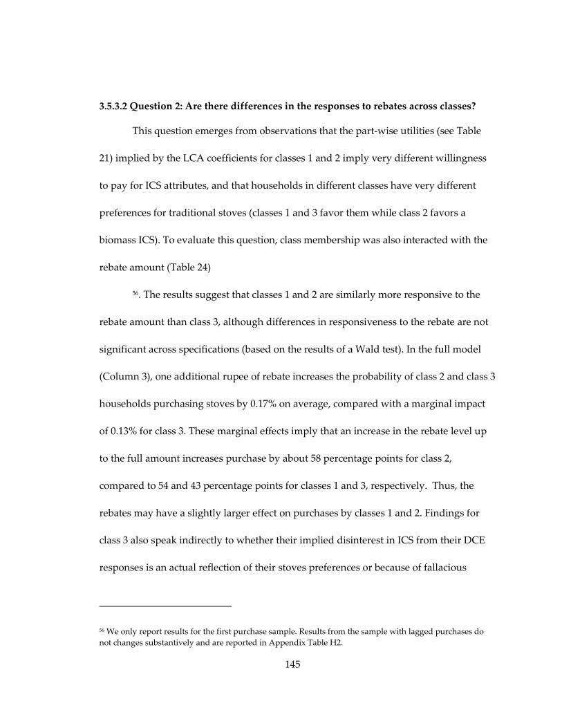
145
3.5.3.2 Question 2: Are there differences in the responses to rebates across classes?
This question emerges from observations that the part-wise utilities (see Table
21) implied by the LCA coefficients for classes 1 and 2 imply very different willingness
to pay for ICS attributes, and that households in different classes have very different
preferences for traditional stoves (classes 1 and 3 favor them while class 2 favors a
biomass ICS). To evaluate this question, class membership was also interacted with the
rebate amount (Table 24)
56. The results suggest that classes 1 and 2 are similarly more responsive to the
rebate amount than class 3, although differences in responsiveness to the rebate are not
significant across specifications (based on the results of a Wald test). In the full model
(Column 3), one additional rupee of rebate increases the probability of class 2 and class 3
households purchasing stoves by 0.17% on average, compared with a marginal impact
of 0.13% for class 3. These marginal effects imply that an increase in the rebate level up
to the full amount increases purchase by about 58 percentage points for class 2,
compared to 54 and 43 percentage points for classes 1 and 3, respectively. Thus, the
rebates may have a slightly larger effect on purchases by classes 1 and 2. Findings for
class 3 also speak indirectly to whether their implied disinterest in ICS from their DCE
responses is an actual reflection of their stoves preferences or because of fallacious
56 We only report results for the first purchase sample. Results from the sample with lagged purchases do not changes substantively and are reported in Appendix Table H2.
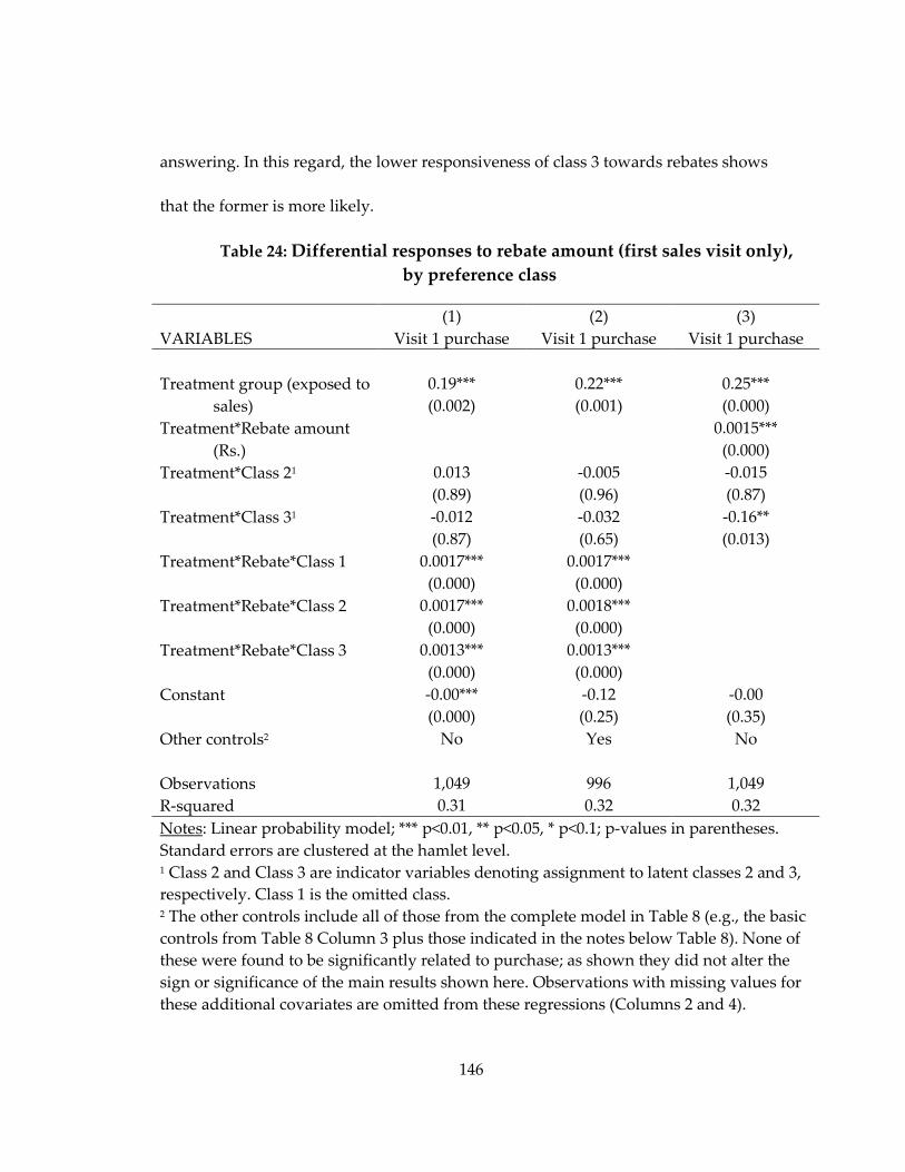
146
answering. In this regard, the lower responsiveness of class 3 towards rebates shows
that the former is more likely.
Table 24: Differential responses to rebate amount (first sales visit only),
by preference class
(1) (2) (3) VARIABLES Visit 1 purchase Visit 1 purchase Visit 1 purchase Treatment group (exposed to 0.19*** 0.22*** 0.25***
sales) (0.002) (0.001) (0.000) Treatment*Rebate amount 0.0015***
(Rs.) (0.000) Treatment*Class 21 0.013 -0.005 -0.015
(0.89) (0.96) (0.87) Treatment*Class 31 -0.012 -0.032 -0.16**
(0.87) (0.65) (0.013) Treatment*Rebate*Class 1 0.0017*** 0.0017*** (0.000) (0.000) Treatment*Rebate*Class 2 0.0017*** 0.0018*** (0.000) (0.000) Treatment*Rebate*Class 3 0.0013*** 0.0013*** (0.000) (0.000) Constant -0.00*** -0.12 -0.00
(0.000) (0.25) (0.35) Other controls2 No Yes No
Observations 1,049 996 1,049 R-squared 0.31 0.32 0.32 Notes: Linear probability model; *** p<0.01, ** p<0.05, * p<0.1; p-values in parentheses. Standard errors are clustered at the hamlet level. 1 Class 2 and Class 3 are indicator variables denoting assignment to latent classes 2 and 3, respectively. Class 1 is the omitted class. 2 The other controls include all of those from the complete model in Table 8 (e.g., the basic controls from Table 8 Column 3 plus those indicated in the notes below Table 8). None of these were found to be significantly related to purchase; as shown they did not alter the sign or significance of the main results shown here. Observations with missing values for these additional covariates are omitted from these regressions (Columns 2 and 4).
147
3.5.3.3 Question 3: Do specific preference types favor the electric stove relative to the
biomass-burning ICS?
To address this question, we consider purchase of the different ICS types, using a
multinomial logit model. Based on the results obtained from question 1, we expect class
1 and 2 households should prefer ICS over class 3 households. It is less clear, however, if
class 1 or class 2 households would be more likely to adopt electric vs. biomass-burning
stoves. On the one hand, class 2 households dislike traditional stoves and have a greater
willingness to pay for all ICS attributes, as discussed above. Yet class 1 households place
greater weight on smoke emissions relative to other ICS attributes, and these are
reduced to zero inside the house by the electric stoves. In addition, the improved
biomass stoves that were offered to the households are more expensive, suggesting that
the more price sensitive class 1 households may prefer the electric ICS. Both
accommodate a single pot, but they differ in terms of fuel costs (the electric stove is more
expensive to operate).
The results are shown in Table 25.57 Our first observation is that class 1
households are most likely to purchase the electric ICS (Columns 2 and 4); when
including all controls, class 1 households are 7% and 13% more likely to purchase this
57 We again only report results for the first purchase sample. Results from the sample with lagged purchases do not differ by much and are reported in Appendix Table H3.

148
stove than classes 2 and 3, respectively.58 In contrast, class 2 households appear more
likely to purchase the biomass-burning ICS on average (Columns 1 and 3); specifically,
they are 8% and 6% more likely to purchase a biomass ICS than classes 1 and 3,
respectively. These results indicate that class 2 households prefer biomass-burning ICS’
over classes 1 and 3, while class 1 households prefer the electric ICS, which is consistent
with the DCE results. As with overall purchase, very few other covariates explain the
differences in purchase rates across technologies. Households in the general caste
category are somewhat more likely to select a biomass-burning stove, while those who
spend more time cooking with traditional stoves are more likely to purchase an electric
one.
We also added the interacted rebate variables to the full model to test if the
classes have different sensitivity to the rebate amount for these different types of stoves.
In Column 5, we see that class 2 is most responsive to the rebate amount for the biomass
stove; the differences between Rc2 and the other two interacted rebate coefficients are
statistically significant. We also note in Column 6 that class 3 households are least
responsive to the rebate for the electric ICS, and class 1 households (the omitted
category) are most responsive. Taken together, these results suggest that relative distaste
for smoke emissions and greater price sensitivity of class 1 households may play a
stronger role in motivating the purchase of electric stoves than the biomass ICS.
58 These marginal effects are evaluated at the mean value of other covariates.

149
Table 25: ICS choice among households exposed to sales intervention, by
latent class (marginal effects)
(1) (2) (3)
Basic +Rebate & Controls +Rebate-class interactions
VARIABLES Biomass
ICS Electric
ICS Biomass
ICS Electric
ICS Biomass
ICS Electric
ICS Rebate amount (Rs.)
0.00068*** 0.00094*** 0.00057***
0.0015***
(0.000) (0.000) (0.002) (0.000) Class 21 0.083** -0.062 0.080** -0.074
(0.011) (0.18) (0.022) (0.15) Class 31 0.028 -0.14*** 0.022 -0.13***
(0.34) (0.000) (0.40) (0.002) Rebate*Class 2 0.00034** -0.00033 (0.013) (0.18)
Rebate*Class 3
0.00013 -0.00068**
* (0.24) (0.002) Other controls2 No Yes Yes
Observations 761 721 721 Pseudo-R2 0.012 0.12 0.12
Notes: Multinomial logit model using initial purchase decision only; we report marginal effects at the mean of the sample covariates; *** p<0.01, ** p<0.05, * p<0.1; p-values in parentheses. Standard errors are clustered at the hamlet level. 1 Class 2 and Class 3 are indicator variables denoting assignment to latent classes 2 and 3, respectively. Class 1 is omitted.
2 The other controls include all of those from the complete model in Table 8 (e.g., the basic controls from Table 8 Column 3 plus those indicated in the notes below Table 8). Few of these were found to be significantly related to purchase; as shown they did not alter the sign or significance of the main results shown here. Observations with missing values for these additional covariates are omitted from these regressions (Columns 2 and 4).

150
3.5.3.4 Question 4: Are specific preference types more likely to use the ICS?
Up to this point, our attention has been focused on ICS purchase decisions, but
the benefits of ICS only come with sustained use (McCracken et al., 2007, Hanna et al.,
2012). We explore the short-term sustainability of ICS usage by using self-reported daily
usage of households’ ICS during the follow-up survey conducted several months after
the sales campaign. In interpreting the results that follow, however, it should be noted
that 74 of the original 1063 households (7.0%) were lost from the sample at follow-up
(Figure 9). Although attrition is not significantly correlated with treatment status, a
slightly smaller percentage of households receiving the high rebate (4.0% vs. 7.8% in the
low rebate group) during the intervention were lost to follow-up. In addition, attrition
may affect the generalizability of our results. Households lost to follow-up were smaller,
more likely to be female-headed, and tended to be less reliant on traditional stoves, as
measured by time spent cooking, fuel consumption, and time spent collecting fuel at
baseline (results available upon request).
Conditional on purchasing ICS, preferences from the DCE are not significantly
correlated with use (Table 26). The analysis of use also confirms findings in the literature
that highlight that ICS ownership often does not necessarily equate to use. In column 1,
for example, we can tell from the intercept that only about 56% of purchasers in the
omitted class (class 1) use the ICS on a daily basis. The full model in column 3 also
shows that the randomized rebate amount is positively associated with use, which

151
suggests that the conditional rebate promised to users at the time of the third sales visit
may perhaps have helped to incentivize longer-term use.59 This effect translates into a
0.1 percentage point for every rupee of rebate. We also separately analyzed electric and
biomass ICS to consider variation in use by stove type. The results are shown in
Columns 4 and 5; the results are similar to the previous analyses in that the preference
classes are no correlated with daily usage of either stove.
59 Other explanations are also possible, for example the presence of income effects, but our experiment was not designed to differentiate among such possibilities.

152
Table 26: ICS use conditional on purchase, by latent class
(1) (2) (3) (4) (5)
Basic +Rebate +SES
Electric ICS
Biomass ICS
VARIABLES Daily use Daily use Daily use Daily use Daily use Rebate amount (Rs.) 0.001*** 0.001*** 0.000 0.001**
(0.005) (0.004) (0.164) (0.041)
Electricity supply -0.006 -0.005 0.009 (hr/day) (0.103) (0.202) (0.118)
Class 2 -0.072 -0.080 -0.103 -0.103 0.039
(0.388) (0.331) (0.207) (0.223) (0.797)
Class 3 -0.033 -0.013 -0.031 -0.014 -0.139
(0.549) (0.820) (0.566) (0.802) (0.252)
Constant 0.559*** 0.385*** 0.558*** 0.630*** 0.413*
(0.000) (0.000) (0.000) (0.000) (0.094)
Other controls2 No No Yes Yes Yes
Observations 386 386 381 303 116 R-squared 0.003 0.027 0.050 0.037 0.115 Notes: Linear probability model using all households that purchased ICS; *** p<0.01, ** p<0.05, * p<0.1; p-values in parentheses. Standard errors are clustered at the hamlet level. 1 Class 2 and Class 3 are indicator variables denoting assignment to latent classes 2 and 3, respectively. Class 1 is omitted.
2 The other controls include all of those from the complete model in Table 8 (e.g., the basic controls from Table 8 Column 3 plus those indicated in the notes below Table 8). Very few of these were found to be significantly related to purchase; as shown they did not alter the sign or significance of the main results shown here. Observations with missing values for these additional covariates are omitted from these regressions (Columns 2 and 4).

153
3.6 Discussion
Field practitioners and policymakers are often stumped when households choose
to not adopt or use seemingly superior technologies that can improve their health and
economic outcomes. These seemingly irrational behaviors have set off a new wave of
studies that attempt to shed light on this puzzle. Nowhere does the adoption puzzle
appear more challenging than in India, where progress has been slow despite several
decades of promotion interventions and the largest potential market for ICS in the
world. This study adds to this effort in a different way by showing that latent
preferences, as revealed through responded stated choices in a discrete choice
experiment of different stove options, relate to actual revealed purchases of distinct
types of ICS. To the best of our knowledge, ours is the first study to explore the mapping
of preferences for any technology elicited through a DCE, to revealed preferences.
Our sample for this comparison consists of roughly 1,050 households living in
rural communities in two districts of Uttarakhand, India, three quarters of whom were
randomly assigned to receive stove sales visits during which two ICS options were
offered to them for purchase. From the DCE, we find that treated households, on
average, respond as expected to the attributes of ICS, favoring those with reduced fuel
requirements, smoke emissions and greater convenience (though the latter two
attributes receive more weight relative to the fuel requirement). On average, they also
appear to favor traditional stoves (rather than the ICS options), all other attributes being

154
equal. Yet these average results mask important heterogeneity in households’
preferences, which we further explore using latent class analysis of these household
choices. The LCA identifies two classes of households, comprising 27% and 20% of the
sample, respectively, who appear differentially ‘interested’ in the features of ICS,
whereas a third class of respondents is generally ‘uninterested’ by these attributes (52%
of households). Within the first two classes, class 1 appears to place much greater
relative weight on smoke emissions reductions than on the other attributes, whereas
class 2 is less price sensitive and values positive changes in all three ICS attributes.
Closer examination of the make-up of each class shows that the ‘uninterested’ class
mainly consists of lower-SES households who lack knowledge on ICS in general and on
the harmful effects of smoke inhalation.
We then consider whether the analyses of stated preferences based on responses
in the DCE map to actual purchase decisions during a randomized stove promotion
intervention. Specifically, our analyses investigate the link between preference class and
the a) likelihood of immediate and lagged ICS purchase, b) responsiveness to price
incentives, and c) the choice of more efficient biomass versus electric ICS stoves. Our
first important result is that the ‘uninterested’ class is less likely to purchase ICS on
average despite the fact that the stove promotion included intensive information
provision and household-level stove demonstrations. This suggests that significant
barriers exist in getting such households, who comprise a majority of our sample, to

155
adopt a new unknown technology such as an ICS. The silver lining in these results,
however, is that class membership becomes less predictive once lagged purchases are
included, which suggests that these class 3 households became more likely to adopt an
ICS during later visits from the sales team. And while our sample was not developed to
allow determination of the precise mechanism behind these changes in decisions, this
result provides hope that such ‘disinterested’ households can with time be convinced to
purchase stoves.
Second, we find that households in different classes respond somewhat
differently to price incentives. In particular, class 2 households appear most (though not
significantly so in the statistical sense) responsive to incentives; these households were
also deemed most likely to adopt ICS based on the results of the LCA. Third, we note
that the class 1 households who placed the greatest relative weight on reduced smoke
emissions relative to a change in other ICS attributes, and who had lower WTP for the
improved biomass stoves offered in the DCE, are most likely to adopt an electric ICS,
which is both cheaper and offers the possibility of eliminating household emissions from
cooking. The predictive power of preference class is retained even when controlling for a
large set of household baseline covariates that have been found in previous literature to
be related to clean stove and fuel use. Lastly, we attempt to distinguish between
adoption and usage by examining if the preference classes have any predictive power on
daily usage of the ICS as reported by households a few months after purchase. We find

156
no correlation between classes and usage. This is perhaps unsurprising given that the
DCE was not designed to elicit information on usage. More importantly, one plausible
interpretation of this result is that there are different conditions governing adoption and
usage decision. A related body of work that has tackled this subject is the recreational
site visit model (e.g. see Phanuef, 2013) where the decision is framed as an
intensive/extensive margin decision. The extensive decision in this case is whether to
adopt ICS and the intensive decision is how often to use the ICS. Numerous approaches
can then be used to solve for the optimal solution of adoption and usage. Following the
approach summarized in Phanuef (2013), we can combine both use and adoption
decisions in the same utility function and use Kuhn-Tucker conditions to solve. Another
plausible approach is to model the use and adoption decision into separately. Towards
this end, an interesting and useful extension of this study is to examine in-depth the
different conditions governing adoption and usage of ICS.
In conclusion, these findings offer considerable new information and insights
that could be incorporated into planning of future ICS promotion efforts, as well as for
other similar quasi-public goods. An oft-neglected feature of the challenge of
environmental health goods provision in low-income settings is that the government, or
socially-minded micro-institutions, must frequently act as the primary suppliers to local
beneficiaries, which typically results in limited (or no) options for consumers. Private
markets naturally meet heterogeneous demand through market segmentation and

157
product differentiation, but the competitive forces that drive such innovations may be
lacking when markets – such as those for ICS – are thin. In addition, NGOs and
governments are often tempted to pick specific solutions based on sound technical
criteria (e.g., an emissions profile), a model that has failed over and over in multiple
sectors (Pritchett & Woolcock 2004). By clearly demonstrating the implications that
latent (and typically unobserved) preferences have for purchases of ICS, our work points
to the need for offering beneficiary households choices rather than prescribing specific
solutions that may not align with their needs. Non-biomass burning technologies such
as electric stoves, which promise greater savings of solid fuel and lower household
emissions, should receive serious consideration in such promotion efforts.

158
Appendix A
Second stage of sorting model with different exclusion distance
(1) (2) 30 km 100 km
VARIABLES Adjusted utility Adjusted utility log(PM2.5) -0.154 -0.140**
(0.522) (0.043) Crime index -0.152* -0.148**
(0.078) (0.044) Health facilities 0.025* 0.025*
(0.097) (0.100) Schools 0.022 0.022
(0.570) (0.576) log(population density) -0.009 -0.010
(0.549) (0.472)
Observations 174 174 R-squared 0.060 0.061 p-value in parentheses *** p<0.01, ** p<0.05, * p<0.1

159
Appendix B
Property hedonic OLS estimation using same data
VARIABLES Log(rent) Log PM2.5 0.083***
(0.000) Size (m2) 0.001***
(0.000) Number of rooms 0.034***
(0.000) House type 1 (Single unit) a -0.227
(0.154) House type 2 (Duplex)a -0.239
(0.133) House type 3 (Multiple units) a -0.244
(0.126) House type 4 (On stilts)a -0.278*
(0.082) House type 5 (Apartments)a -0.223
(0.218) Floor type 1 (Ceramic/Marble) b 0.163***
(0.000) Floor type 2 (Tiles) b 0.070***
(0.000) Floor type 3 (Cement/Brick)
b 0.029** (0.033)
Floor type 4 (Lumber) b 0.012 (0.534)
Floor type 5 (Bamboo)b -0.017 (0.696)
Wall type 1 (Masonry) c 0.127*** (0.000)
Wall type 2 (Lumber)c 0.041*** (0.006)
Roof type 1 (Concrete) d 0.154*** (0.000)
Roof type 2 (Wood) d 0.127*** (0.000)
Roof type 3 (Metal) d 0.071*** (0.004)
Roof type 4 (Shingles) d 0.104*** (0.000)
Roof type 5 (Asbestos)d 0.107*** (0.000)
Owner 0.035*** (0.000)
Constant 0.682*** (0.000)
Observations 11,883 R-squared 0.275 p-value in parentheses a Excluded category is multi-story units which are the most valuable housing type; b Excluded category is dirt; c Excluded category is bamboo/mat d Excluded category is foliage/grass

160
Appendix C
Property hedonic estimation using same data (Log PM2.5 instrumented using source-, wind-, and distance- based instrument)
VARIABLES Log(rent) Log PM2.5 -0.163**
(0.018) Size (m2) 0.001***
(0.000) Number of rooms 0.034***
(0.000) House type 1 (Single unit) a -0.242
(0.129) House type 2 (Duplex)a -0.259
(0.105) House type 3 (Multiple units) a -0.259
(0.106) House type 4 (On stilts)a -0.163**
(0.018) House type 5 (Apartments)a 0.001***
(0.000) Floor type 1 (Ceramic/Marble)
b 0.034*** (0.000)
Floor type 2 (Tiles) b -0.242 (0.129)
Floor type 3 (Cement/Brick) b -0.259 (0.105)
Floor type 4 (Lumber) b -0.259 (0.106)
Floor type 5 (Bamboo)b -0.163** (0.018)
Wall type 1 (Masonry) c -0.285* (0.075)
Wall type 2 (Lumber)c -0.248 (0.174)
Roof type 1 (Concrete) d 0.165*** (0.000)
Roof type 2 (Wood) d 0.068*** (0.000)
Roof type 3 (Metal) d 0.026* (0.051)
Roof type 4 (Shingles) d 0.016 (0.393)
Roof type 5 (Asbestos)d -0.012 (0.791)
Owner 0.131*** (0.000)
Constant 0.037** (0.016)
Observations 11,883 R-squared 0.267 p-value in parentheses *** p<0.01, ** p<0.05, * p<0.1 Province FEs included Standard errors clustered at district level a Excluded category is multi-story units which are the most valuable housing type; b Excluded category is dirt; c Excluded category is bamboo/mat d Excluded category is foliage/grass

161
Appendix D
Results from sorting model without moving costs (Left table – First stage; Right table – Second stage)
VARIABLES log(wage) 2.78***
(0.000)
Households 10,125 Alternatives 174 p-value in parentheses *** p<0.01, ** p<0.05, * p<0.1
VARIABLES Adjusted utility log(PM2.5) -0.214***
(0.001) Crime index 0.011
(0.794) Health facilities -0.033***
(0.000) Schools 0.049**
(0.026) log(population density) -0.003
(0.897)
Observations 174 R-squared 0.020 p-value in parentheses *** p<0.01, ** p<0.05, * p<0.1

162
Appendix E
Repeat of Table 11 using a gestation period of nine months (1) (2) (3) (4) (5) (6) (7)
Basic + District
fixed effects +Parents' education
+Climatic factors
By trimesters
+ Households inputs
+ Households inputs (by trimesters)
VARIABLES Height-for-age z-score AI -2.373** -4.266** -5.698*** -5.728*** -5.537*** AI at first trimester -4.589*** -4.200*** AI at second trimester -5.121* -5.577* AI at third trimester -1.048 0.926 AI at fourth trimester -1.565 -0.795 AI at fifth trimester -1.319 -0.304 Father’s height 0.021*** 0.017*** 0.015*** 0.015*** 0.014*** 0.015*** 0.014*** Mother’s height 0.036*** 0.030*** 0.028*** 0.028*** 0.027*** 0.023*** 0.022*** Father at least high school 0.272** 0.265** 0.253** 0.169 0.168 Mother at least high school 0.147 0.151 0.142 -0.040 -0.065 Precipitation -0.006 -0.002 -0.009 -0.004 Temperature -0.282 -1.148* -0.045 -0.993 Improved sanitation in 1997 0.168 0.175 Uses biomass fuel in 1997 -0.255* -0.257* Improved sanitation in 2000 0.023 0.026 Uses biomass fuel in 2000 -0.249* -0.265* Constant -10.224*** -8.590*** -7.879*** -7.798*** -8.294*** -6.702*** -7.306*** Birth Month FEs Y Y Y Y Y Y Y Districts FEs N Y Y Y Y Y Y Observations 746 746 688 688 688 598 598 R-squared 0.122 0.108 0.131 0.133 0.149 0.144 0.170 Standard errors clustered at district level (not shown) *** p<0.01, ** p<0.05, * p<0.1

163
Appendix F
Repeat of Table 12 using a gestation period of nine months. (1) (2) (3) (4) (5) (6)
VARIABLES Cognitive test Cognitive test
Lung capacity
Lung capacity
Weight-for-age z-score
Weight-for-age z-score
AI -0.403 -3.520 -0.105 AI at first trimester -0.759** -89.502 -2.140 AI at second trimester -0.441 -321.212** 1.047 AI at third trimester -0.541 -211.354* 1.438 AI at fourth trimester -0.369 45.176 0.747 AI at fifth trimester -0.261 -143.316 4.273 Male 0.002 0.003 14.850*** 14.862*** Age (months) 0.004** 0.000 Father at least high school 0.024 0.021 0.327 1.046 0.090 0.075 Mother at least high school 0.050** 0.052** 0.972 -0.086 0.131 0.139 Precipitation 0.001 0.001 -0.205 -0.121 -0.001 0.000 Temperature -0.193 -0.179 35.883 3.820 -0.070 -0.533 Father’s lung capacity 0.079*** 0.081*** Mother’s lung capacity 0.118*** 0.118*** Father’s weight 0.034*** 0.034*** Mother’s weight 0.032*** 0.031*** Constant 0.101 0.558 112.843*** 123.663*** -5.310*** -5.567***
Observations 735 735 690 690 685 685 R-squared 0.039 0.045 0.123 0.151 0.195 0.205 Number of kabupaten 154 154 151 151 151 151 Standard errors clustered at district level (not shown) *** p<0.01, ** p<0.05, * p<0.1
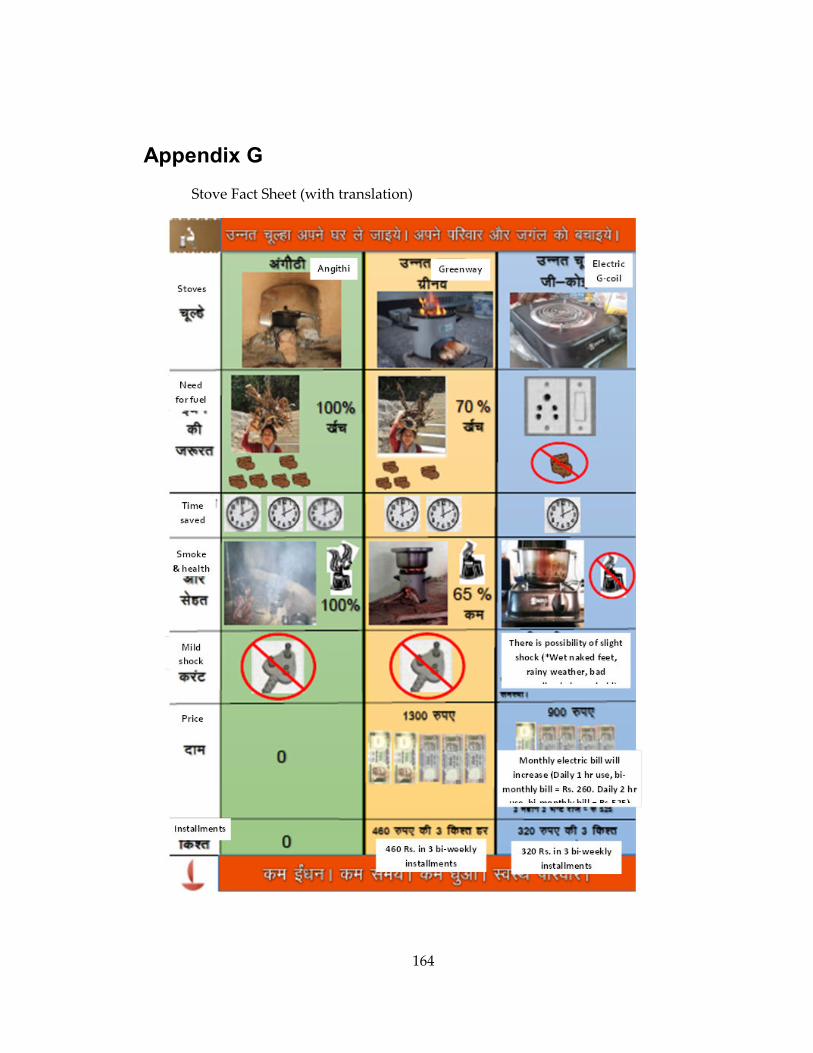
164
Appendix G
Stove Fact Sheet (with translation)

165
Appendix H
Table H1. Analysis of serial non-response and class 3 membership
VARIABLE Serial non-respondent
Other respondent N
Household in class 3 332 245 577
Household not in class 3 0 486 486 N 332 731 1063
Notes: Serial non-respondents are households who selected the traditional stove alternative in the DCE in all 4 choice tasks, no matter the attributes of the ICS options.

166
Table H2: Differential responses to rebate amount and prior institutional presence (all sales visits), by preference class (1) (2) (3) (4)
VARIABLES All
purchases All
purchases All
purchases All
purchases
Treatment group (exposed to sales
0.19*** 0.22*** 0.25*** 0.22***
Treatment*Rebate amount 0.0015***
Electricity supply (hr/day) 0.0062*** 0.0058***
Treatment*Class 21 -0.003 -0.031 -0.005 -0.049
Treatment*Class 31 0.069 0.049 -0.11 0.004
Treatment*Rebate*Class 1 0.0019*** 0.0019*** 0.0019***
Treatment*Rebate*Class 2 0.0020*** 0.0020*** 0.0020***
Treatment*Rebate*Class 3 0.0012*** 0.0012*** 0.0012***
Treatment*NGO*Class 1 0.035
Treatment*NGO*Class 2 0.048
Treatment*NGO*Class 3 0.12
Constant -0.00*** -0.17* -0.00 -0.15
Other controls2 No Yes No Yes
Observations 1,049 996 1,049 996
R-squared 0.34 0.36 0.324 0.36
Notes: Linear probability model; *** p<0.01, ** p<0.05, * p<0.1; p-values in parentheses. Standard errors are clustered at the hamlet level. 1 Class 2 and Class 3 are indicator variables denoting assignment to latent classes 2 and 3, respectively. Class 1 is the omitted class.
2 The other controls include all of those from the complete model in Table 8 (e.g., the basic controls from Table 8 Column 3 plus those indicated in the notes below Table 8). Very few of these were found to be significantly related to purchase; as shown they did not alter the sign or significance of the main results shown here. Observations with missing values for these additional covariates are omitted from these regressions (Columns 2 and 4).
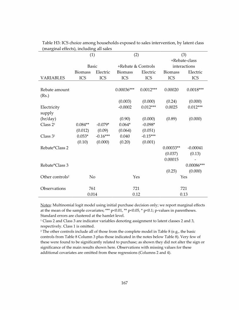
167
Table H3: ICS choice among households exposed to sales intervention, by latent class (marginal effects), including all sales
(1) (2) (3)
Basic +Rebate & Controls +Rebate-class interactions
VARIABLES Biomass
ICS Electric
ICS Biomass
ICS Electric
ICS Biomass
ICS Electric
ICS Rebate amount (Rs.)
0.00036*** 0.0012*** 0.00020 0.0018***
(0.003) (0.000) (0.24) (0.000) Electricity supply
-0.0002 0.012*** 0.0025 0.012***
(hr/day) (0.90) (0.000) (0.89) (0.000) Class 21 0.084** -0.079* 0.064* -0.098*
(0.012) (0.09) (0.064) (0.051) Class 31 0.053* -0.16*** 0.040 -0.15***
(0.10) (0.000) (0.20) (0.001) Rebate*Class 2 0.00033** -0.00041 (0.037) (0.13)
Rebate*Class 3 0.00015 -
0.00086*** (0.25) (0.000) Other controls2 No Yes Yes
Observations 761 721 721 0.014 0.12 0.13
Notes: Multinomial logit model using initial purchase decision only; we report marginal effects at the mean of the sample covariates; *** p<0.01, ** p<0.05, * p<0.1; p-values in parentheses. Standard errors are clustered at the hamlet level. 1 Class 2 and Class 3 are indicator variables denoting assignment to latent classes 2 and 3, respectively. Class 1 is omitted.
2 The other controls include all of those from the complete model in Table 8 (e.g., the basic controls from Table 8 Column 3 plus those indicated in the notes below Table 8). Very few of these were found to be significantly related to purchase; as shown they did not alter the sign or significance of the main results shown here. Observations with missing values for these additional covariates are omitted from these regressions (Columns 2 and 4).

168
Appendix I
Latent class logit
The conditional choice probability of respondent i choosing alternative j in choice
task t, given that she belongs to class s is:
, (H1)
where is a vector of coefficients for the attributes of the alternatives.
Next, the unconditional probability that respondent i belongs to class s is:
. (H2)
Depending on the researcher’s objective, can be a vector of observable
characteristics such as education and income or just a vector of constants. If contains
individual characteristics, this probability expression is expressed as a multinomial form
where the coefficient for the excluded class is normalized to zero. As such, should be
interpreted relative to the excluded class.
Combining these expressions, the probability that respondent i chooses
alternative j in task t is:
. (H3)

169
If we multiply this expression by the probabilities from the other choice tasks, we
recover the probability for choosing a particular sequence of alternatives:
. (H4)
This expression is then summed over the entire sample to arrive at the log
likelihood:
. (H5)
The preference parameters and S – 1 class parameters can be recovered
from this log likelihood function either by maximum likelihood estimation or through
application of the EM algorithm (Green & Hensher, 2003; Train, 2008; Bhat, 1997).
Using Bayes theorem and the parameters from the likelihood function, we then
estimate the conditional probability that a respondent belongs to each class s given her
selection of alternative j:
. (H6)

170
References
Abberger, H., Sanders, B., and Dotzauer, H. (2002). “The development of a community-based approach for an integrated forest fire management system in East Kalimantan, Indonesia”. In P. Moore, D. Ganz, L. Tan, T. Enters, and P. Durst (Eds.), Communities in flames: Proceedings of and international conference on community
involvement in fire management. (pp. 53-65). Bangkok: FAO.
Adair, L. S. (1999). “Filipino children exhibit catch-up growth from age 2 to 12 years”. Journal of Nutrition. 129(6): 1140-8.
Akresh, R., & De Walque, D. (2008). “Armed conflict and schooling: Evidence from the 1994 Rwandan genocide”. World Bank Policy Research Working Paper Series: 4606.
Akresh, R., Verwimp, P., & Bundervoet, T. (2011). “Civil war, crop failure, and child stunting in Rwanda”. Economic Development and Cultural Change. 59(4): 777-810.
Alberini, A., Cropper, M., Fu, T.T., Krupnick, A., Liu, J.T., Shaw, D., and Harrington, W. (1997). “Valuing health effects of air pollution in developing countries: The case of Taiwan”. Journal of Environmental Economics and Management. 34(2): 107-26.
Almond, D., Edlund, L., Li, H., & Zhang, J. (2010). “Long-term effects of early-life development: Evidence from the 1959 to 1961 china famine”. In The Economic
Consequences of Demographic Change in East Asia, NBER-EASE. Volume 19 (pp. 321-345). University of Chicago Press.
Angelsen, A. (1995). “Shifting cultivation and “deforestation”: a study from Indonesia”. World Development. 23(10): 1713-29.
Ashraf, N., B. K. Jack, & E. Kamenica. (2013). “Information and subsidies: Complements or substitutes?” Journal of Economic Behavior & Organization. 88:133–9.
Ashraf, N., J. Berry, & J. M. Shapiro. (2010). “Can higher prices stimulate product use? Evidence from a field experiment in Zambia” American Economic Review. 100: 2383–413.
Auffhammer, M., Hsiang, S. M., Schlenker, W., & Sobel, A. (2013). Using weather data and climate model output in economic analyses of climate change. Review of
Environmental Economics and Policy, ret016.

171
Bandan Pusat Statistik. (2006). 2006 Village potential statistics [Data file and code book]. Retrieved from http://library.duke.edu/data/collections/podes/.
Bandan Pusat Statistik. (2011). Consumer price of selected goods and services for housing groups in 66 cities in Indonesia 2010. Jakarta, Indonesia: BPS - Statistics Indonesia
Barker, D.J. (1990). “The fetal and infant origins of adult disease”. BMJ. 301(6761): 1111.
Bartik, T. J. (1987). “The estimation of demand parameters in hedonic price models”. Journal of Political Economy. 95(1): 81-8.
Bateson, P., Barker, D., Clutton-Brock, T., Deb, D., D'Udine, B., Foley, R. A., ... & Sultan, S.E. (2004). “Developmental plasticity and human health”. Nature. 430(6998): 419-21.
Battelle Memorial Institute, and Center for International Earth Science Information Network - CIESIN - Columbia University. (2013). Global annual average PM2.5 grids
from MODIS and MISR Aerosol Optical Depth (AOD). Palisades, NY: NASA Socioeconomic Data and Applications Center (SEDAC). Retrieved from http://dx.doi.org/10.7927/H4H41PB4/
Bayer, P., F. Ferreira, and R. McMillan. (2007). “A unified framework for measuring preferences for schools and neighborhoods”. Journal of Political Economy. 115(4): 588-638.
Bayer, P., McMillan, R., and Rueben, K. S. (2004). “What drives racial segregation? New evidence using census microdata”. Journal of Urban Economics. 56(3): 514-35.
Bayer, P., N. Keohane, and C. Timmins. (2009). “Migration and hedonic valuation: The case of air quality”. Journal of Environmental Economics and Management. 58(1): 1-14.
Bedi, A. S., and Garg, A. (2000). “The effectiveness of private versus public schools: The case of Indonesia”. Journal of Development Economics. 61(2): 463-494.
Bensch, G., & Peters, J. (2014). “The intensive margin of technology adoption-Experimental evidence on improved cooking stoves in rural Senegal”. Ruhr
Economic Paper (494).

172
Bensch, G., Grimm, M., & Peters, J. (2014). Why Do Households Forego High Returns
from Technology Adoption: Evidence from Improved Cook Stoves in Burkina Faso. Ruhr Economic Papers #498. Essen, Germany.
Berry, J., G. Fischer, & R.P. Guiteras. (2012) “Eliciting and utilizing willingness to pay:
Evidence from field trials in Northern Ghana” Working Paper.
Bertrand, M., & Mullainathan, S. (2001). “Do people mean what they say? Implications for subjective survey data”. American Economic Review Papers and
Proceedings of the Hundred Thirteenth Annual Meeting of the American Economic
Association. 91(2): 67-72.
Besley, T. & Case, A. (1993). “Modeling technology adoption in developing countries”. American Economic Review Papers and Proceedings of the Hundred and Fifth
Annual Meeting of the American Economic Association. 83(2): 396-402
Bharadwaj, P., Gibson, M., Zivin, J. G., & Neilson, C. A. (2014). Gray Matters: Fetal
Pollution Exposure and Human Capital Formation (No. w20662). National Bureau of Economic Research.
Bhojvaid, V., Jeuland, M., Kar, A., Lewis, J., Pattanayak, S., Ramanathan, N., . . . Rehman, I. ( 2013). “How do people in rural India perceive improved stoves and clean fuel? Evidence from Uttar Pradesh and Uttarakhand” (Under Review).
Bobak, M., & Leon, D. A. (1992). “Air pollution and infant mortality in the Czech Republic, 1986-88”. The Lancet. 340(8826): 1010-14.
Bohra-Mishra, P., Oppenheimer, M., & Hsiang, S. M. (2014). Nonlinear permanent migration response to climatic variations but minimal response to disasters. Proceedings of the National Academy of Sciences, 201317166.
Bond, T., C. Venkataraman and O. Masera (2004). “Global atmospheric impacts of residential fuels.” Energy for Sustainable Development. 8(3): 20-32.
Borghans, L., Duckworth, A.L., Heckman, J.J., & Ter Weel, B. (2008). "The economics and psychology of personality traits". Journal of Human Resources. 43(4): 972-1059.
Bouthillier, L., Vincent, R., Goegan, P., Adamson, I. Y., Bjarnason, S., Stewart, M., ... & Kumarathasan, P. (1998). “Acute effects of inhaled urban particles and ozone: lung morphology, macrophage activity, and plasma endothelin-1”. American Journal

173
of Pathology. 153(6): 1873-84.
Brown, J.N., and Rosen, H.S. (1982). “On the estimation of structural hedonic price models.” Econometrica. 50(3): 765-68.
Bruce, N., Rehfuess, E., Mehta, S., Hutton, G., & Smith, K.R. (2006). Chapter 42: Indoor Air Pollution. In D. e. a. Jamison (Ed.), Disease control priorities in developing
countries: WHO.
Cameron, N., Preece, M. A., & Cole, T. J. (2005). “Catch-up growth or regression to the mean? Recovery from stunting revisited”. American Journal of Human Biology. 17(4): 412-17.
Cárdenas, J.C., Chong, A., & Ñopo, H. (2013). “Stated social behavior and revealed actions: Evidence from six Latin American countries”. Journal of Development
Economics. 104: 16-33.
Carson, R.T, Flores, N.E, Martin, K.M, & Wright, J.L. (1996). “Contingent valuation and revealed preference methodologies: comparing the estimates for quasi-public goods”. Land Economics. 72(1): 80-99.
Casabonne, U., & Kenny, C. (2012). “The best things in life are (nearly) free: technology, knowledge, and global health”. World Development. 40(1): 21-35.
Chang, T., Zivin, J. S. G., Gross, T., & Neidell, M. J. (2014). Particulate pollution and
the productivity of pear packers. National Bureau of Economic Research (No. w19944).
Chay, K.Y., & Greenstone, M. (2005). “Does air quality matter? Evidence from the housing market”. Journal of Political Economy. 113(2): 376-424.
Chen, Y., & Zhou, L.A. (2007). “The long-term health and economic consequences of the 1959–1961 famine in China”. Journal of Health Economics. 26(4): 659-81.
children’s future, ed. M.E. Young. 39–83. Amsterdam: Elsevier.
Choi, S.W., & Friso, S. (2010). “Epigenetics: a new bridge between nutrition and health”. Advances in Nutrition: An International Review Journal. 1(1): 8-16.
Cochrane, M. A. (2003). “Fire science for rainforests”. Nature. 421(6926): 913-9.

174
Cochrane, M.A., Alencar, A., Schulze, M.D., Souza, C.M., Nepstad, D.C., Lefebvre, P., & Davidson, E.A. (1999). “Positive feedbacks in the fire dynamic of closed canopy tropical forests”. Science. 284(5421): 1832-5.
Cohen, J. & P. Dupas. (2010). “Free distribution or cost-sharing? Evidence from a randomized malaria prevention experiment” Quarterly Journal of Economics. 125:1–45.
Colvin, J., Lewis, J.J., Pattanayak, S.K., Sasser, E., & Vergnano, E. (2013). “Analysis of
global stove sales patterns”. Durham, USA: Working Paper, Cookstove Research Initiative, Duke University.
Currie, J., & Vogl, T. (2013). “Early-life health and adult circumstance in developing countries”. Annual Review of Economics. 5(1): 1-36.
Dahl, G. B. (2002). “Mobility and the return to education: Testing a Roy model with multiple markets”. Econometrica. 70(6): 2367-420.
Dasgupta, P. (2013). “The nature of economic development and the economic development of nature”. Available at SSRN: http://ssrn.com/abstract=2352914
Dauvergne, P. (1998). “The political economy of Indonesia's 1997 forest fires”. Australian Journal of International Affairs. 52(1): 13-7.
Davies, S.J., and Unam, L. (1999). “Smoke-haze from the 1997 Indonesian forest fires: effects on pollution levels, local climate, atmospheric CO2 concentrations, and tree photosynthesis”. Forest Ecology and Management. 124(2): 137-44.
Dercon, S., & Porter, C. (2014). “Live aid revisited: Long-term impacts of the 1984 Ethiopian famine on children”. Journal of the European Economic Association. 12(4): 927-48.
Diamond, P.A., & Hausman, J.A. (1994). “Contingent valuation: Is some number better than no number?”. The Journal of Economic Perspectives. 8(4): 45-64.
Du, X., and Mendelsohn, R. O. (2011). “Estimating the value of the reduction in air pollution during the Beijing Olympics”. Environment and Development Economics. 16(06): 735-749.
Duflo, E., Greenstone, M., & Hanna, R. (2008). “Indoor air pollution, health and economic well-being”. SAPI EN. S. Surveys and Perspectives Integrating Environment

175
and Society(1.1).
Dupas, P. (2014). “Short-run subsidies and long-run adoption of new health products: Evidence from a field experiment” Econometrica. 82:197–228.
Edwards, S. (1996). “Why are Latin America's savings rates so low? An international comparative analysis”. Journal of Development Economics. 51(1): 5-44.
Emmanuel, S.C. (2000). “Impact to lung health of haze from forest fires: the Singapore experience”. Respirology. 5(2): 175-82.
Epple, D. (1987). “Hedonic prices and implicit markets: estimating demand and supply functions for differentiated products”. Journal of Political Economy. 95(1): 59-80.
Eskeland, G.S., and Jimenez, E. (1992). “Policy instruments for pollution control in developing countries”. World Bank Research Observer. 7(2): 145-69.
Ezzati, M, & Kammen, DM. (2001). “Indoor air pollution from biomass combustion and acute respiratory infections in Kenya: an exposure-response study”. The Lancet.
358(9282): 619-24.
Fatah, L., and Udiansyah. (2009). “An assessment of forest management options for
preventing forest fire in Indonesia”. EEPSEA Research Report No. 2009-RR9.
Ferraro, P.J., K. Lawlor, K.L., Mullan, and S.K., Pattanayak. (2012). “Forest figures: A review of ecosystem services valuation and policies in developing countries”. Review of Environmental Economics and Policy. 6(1): 20-44.
Fischer, G., D. Karlan, M. McConnell, & P. Raffler. (2014). “To Charge or Not to
Charge: Evidence from a Health Products Experiment in Uganda”. Working Paper.
Fitrani, F., Hofman, B., and Kaiser, K. (2005). “Unity in diversity? The creation of new local governments in a decentralising Indonesia”. Bulletin of Indonesian
Economic Studies. 41(1): 57-79.
Food and Agriculture Organization of the United Nations. (2006). “Global Forest
Resources Assessment 2005” FAO Forestry Paper 147.
Frankenberg, E., McKee, D., and Thomas, D. (2005). “Health consequences of forest fires in Indonesia”. Demography. 42(1): 109-29.

176
Fung, W., & Ha, W. (2009). “Intergenerational effects of the 1959-61 China famine”. In Risk, Shocks, and Human. Development: On the Brink, edited by R. Fuentes and P. Seck. 222–254.
GACC. (2010). Secretary Clinton Announces Global Alliance for Clean Cookstoves.
GACC. (2011). Igniting change: A strategy for universal adoption of clean cookstoves and fuels. Washington: Global Alliance for Clean Cookstoves.
GACC. (2012). 2012 Results Report: Sharing Progress on the Path to Adoption of Clean Cooking Solutions. Washington: Global Alliance for Clean Cookstoves.
Germer, J., & Sauerborn, J. (2008). “Estimation of the impact of oil palm plantation establishment on greenhouse gas balance”. Environment, Development and
Sustainability. 10(6): 697-716.
Ghosh, A., and Mukherji, A. (2014). “Air Pollution and Respiratory Ailments among Children in Urban India: Exploring Causality”. Economic Development and
Cultural Change. 63(1): 191-222.
Gicquel, C., El-Osta, A., & Le Bouc, Y. (2008). “Epigenetic regulation and fetal programming”. Best Practice & Research Clinical Endocrinology & Metabolism. 22(1): 1-16.
Glinianaia, S.V., Rankin, J., Bell, R., Pless-Mulloli, T., & Howel, D. (2004). “Particulate air pollution and fetal health: a systematic review of the epidemiologic evidence”. Epidemiology. 15(1): 36-45.
Glover, D., & Jessup, T. (1999). Indonesia's fires and haze: The cost of catastrophe. Singapore: Institute of Southeast Asian Studies.
Glover, D., & Jessup, T. (2006). The Indonesian fires and haze of 1997: The economic toll. Singapore: Institute of Southeast Asian Studies.
Gluckman, P. D., & Hanson, M. A. (2004). “Living with the past: evolution, development, and patterns of disease”. Science. 305(5691): 1733-6.
Gluckman, P. D., Hanson, M. A., & Beedle, A. S. (2007). “Early life events and their consequences for later disease: a life history and evolutionary perspective”. American Journal of Human Biology. 19(1): 1-19.

177
Goldammer, J.G., Frost, P.G.H, Jurvelius, M., Kamminga, E.M., Kruger, T., Moody, S.I., and Pogeyed, M. (2002). “Community participation in integrated forest fire management: experiences from Africa, Asia, and Europe” In P. Moore, D. Ganz, L. Tan, T. Enters, and P. Durst (Eds.), Communities in flames: Proceedings of and
international conference on community involvement in fire management. (pp. 33-52). Bangkok: FAO.
Gonzalez, F., Leipnik, M., and Mazumder, D. (2013). “How much are urban residents in Mexico willing to pay for cleaner air?”. Environment and Development
Economics. 18(3): 354-79.
Government of the Philippines. Republic Act No. 8749. An act providing for a comprehensive air pollution control policy and other purposes. (1999)
Government of Vietnam. Decision No. 64/2003. Approving the plan for thoroughly handling establishments which cause serious environmental pollution. (2003)
Grandey, B.S., Stier, P., and Wagner, T.M. (2013). “Investigating relationships between aerosol optical depth and cloud fraction using satellite, aerosol reanalysis and general circulation model data”. Atmospheric Chemistry and Physics. 13(6): 3177-3184.
Grandstaff, S. and Dixon, J.A. (1986). “Evaluation of Lumpinee park in Bangkok, Thailand”. In Economic Valuation Techniques for the Environment: A Case Study
Workbook (pp. 121-40). Baltimore, MD: Johns Hopkins University Press.
Greenstone, M., and R. Hanna. (2014). "Environmental Regulations, Air and Water Pollution, and Infant Mortality in India." American Economic Review. 104(10): 3038-72.
Grossman, G.M. and Krueger, A.B. (1995). “Economic growth and the environment”. Quarterly Journal of Economics. 110(2): 353-77.
Grossman, M. (1972). “The Demand for Health: A Theoretical and Empirical Investigation”. NBER Books. University of Chicago Press: Chicago, IL.
Ha, E.H., Hong, Y.C., Lee, B.E., Woo, B.H., Schwartz, J., & Christiani, D.C. (2001). “Is air pollution a risk factor for low birth weight in Seoul?”. Epidemiology. 12(6): 643-648.
Hanna, R., & Oliva, P. (2014). “The effect of pollution on labor supply: Evidence

178
from a natural experiment in Mexico City”. Journal of Public Economics. 122: 68-79
Hanna, R., Duflo, E., & Greenstone, M. (2012). “Up in Smoke: The Influence of
Household Behavior on the Long-Run Impact of Improved Cooking Stoves”: National Bureau of Economic Research (No. w18033).
Hansen, M.C., Potapov, P.V., Moore, R., Hancher, M., Turubanova, S.A., Tyukavina, A., ... and Townshend, J.R.G. (2013). “High-resolution global maps of 21st-century forest cover change”. Science. 342(6160): 850-3.
Hausman, J. (2012). “Contingent valuation: from dubious to hopeless”. The Journal
of Economic Perspectives. 26(4): 43-56.
Health Effects Institute (2010). “Public health and air pollution in Asia (PAPA): Coordinated studies of short-term exposure to air pollution and daily mortality in four cities”. HEI Research Report 154. Boston, MA: Health Effects Institute.
Heckman, J.J. (1979). “Sample selection bias as a specification error”. Econometrica. 47(1): 153-161.
Heckman, James J. (2001). “Micro data, heterogeneity, and the evaluation of public policy: Nobel lecture”. Journal of Political Economy. 109(4): 673-748.
Heil, A., & Goldammer, J. (2001). “Smoke-haze pollution: a review of the 1997 episode in Southeast Asia”. Regional Environmental Change. 2(1): 24-37.
Heil, A., and Goldammer, J. (2001). “Smoke-haze pollution: A review of the 1997 episode in Southeast Asia”. Regional Environmental Change. 2(1): 24-37.
Heutel, G., and Ruhm, C. J. (2013). “Air pollution and procyclical mortality” National Bureau of Economic Research. (No. w18959).
Hoddinott, J., & Kinsey, B. (2001). “Child growth in the time of drought”. Oxford
Bulletin of Economics and Statistics. 63(4): 409-36.
Hsu, N.C., Herman, J.R., Torres, O., Holben, B.N., Tanre, D., Eck, T.F., ... & Lavenu, F. (1999). “Comparisons of the TOMS aerosol index with Sun-photometer aerosol optical thickness: Results and applications”. Journal of Geophysical Research. 104(D6): 6269-79.
IBRD (1992). World Development Report 1992. Development and the Environment. New

179
York: Oxford University Press.
Isen, A., Rossin-Slater, M., & Walker, W.R. (2014). Every Breath You Take-Every Dollar
You'll Make: The Long-Term Consequences of the Clean Air Act of 1970. National Bureau of Economic Research (No. w19858).
Jack, B.R., Oliva, P., Severen, C., Walker, E., Bell, S. (2015). “Technology adoption
under certainty”. Working paper.
Jacoby, H.G., & Skoufias, E. (1997). “Risk, financial markets, and human capital in a developing country”. Review of Economic Studies. 64(3): 311-35.
Jayachandran, S. (2009). “Air quality and early-life mortality evidence from Indonesia’s wildfires”. Journal of Human Resources. 44(4): 916-54.
Jenkins, M. W., & Curtis, V. (2005). “Achieving the ‘good life’: Why some people want latrines in rural Benin”. Social Science & Medicine. 61(11): 2446-59.
Jeuland, M., Orgill, J. , Shaheed, A. , & Brown, J. (2013). “A matter of good taste: Investigating preferences for in-house water treatment in peri-urban communities in Cambodia”. Working paper.
Jeuland, M.A., & Pattanayak, S.K. (2012). “Benefits and costs of improved cookstoves: Assessing the implications of variability in health, forest and climate Impacts”. PloS One. 7(2): e30338.
Johansson-Stenman, O., Mahmud, M., & Martinsson, P. (2013). “Trust, trust games and stated trust: Evidence from rural Bangladesh”. Journal of Economic Behavior &
Organization. 95: 286-98.
Kahn, S., and Lang, K. (1988). “Efficient estimation of structural hedonic systems”. International Economic Review. 29(1): 157-66.
Kappos, A. D., Bruckmann, P., Eikmann, T., Englert, N., Heinrich, U., Höppe, P., ... and Wichmann, H. (2004). “Health effects of particles in ambient air”. International Journal of Hygiene and Environmental Health. 207(4): 399-407.
Kim Oanh, N. T., Upadhyay, N., Zhuang, Y. H., Hao, Z. P., Murthy, D. V. S., Lestari, P., ... & Lindgren, E. S. (2006). “Particulate air pollution in six Asian cities: Spatial and temporal distributions, and associated sources”. Atmospheric
environment, 40(18): 3367-3380.

180
Klaiber, H.A., and Phaneuf, D.J. (2010). “Valuing open space in a residential sorting model of the Twin Cities”. Journal of Environmental Economics and Management. 60(2): 57-77.
Kling, C. L., Phaneuf, D. J., & Zhao, J. (2012). “From Exxon to BP: Has some number become better than no number?”. The Journal of Economic Perspectives. 26(4):3-26.
Knottnerus, J.A., Delgado, L.R., Knipschild, P.G., Essed, G.G.M., & Smits, F. (1990). “Haematologic parameters and pregnancy outcome A prospective cohort study in the third trimester”. Journal of Clinical Epidemiology. 43(5): 461-6.
Kochar, A. (1995). “Explaining household vulnerability to idiosyncratic income shocks”. American Economic Review. 85(2): 159-64.
Kojima, M., and Lovei, M. (2001). Urban air quality management - coordinating
transport, environment, and energy policies in developing countries. World Bank Technical Paper no. 508. Pollution Management Series. Washington, D.C: The World Bank.
Kuminoff, N.V., Smith, V.K., and Timmins, C. (2013). “The new economics of equilibrium sorting and policy evaluation using housing markets”. Journal of
Economic Literature. 51(4): 1007-62.
Lee, K. H., Li, Z., Kim, Y. J., & Kokhanovsky, A. (2009). Atmospheric aerosol monitoring from satellite observations: a history of three decades. In Atmospheric
and biological environmental monitoring (pp. 13-38). Springer Netherlands.
Legros, G, Havet, I, Bruce, N, & Bonjour, S. (2009). “The energy access situation in developing countries: a review focusing on the least developed countries and sub-Saharan Africa”. New York: UNDP and WHO.
Levine, D.I, Beltramo, T., Blalock, G., & Cotterman, C. (2013). “What impedes efficient adoption of products? Evidence from randomized variation in sales offers for improved cookstoves in Uganda”. Working Paper.
Lewis, J, Bhojvaid, V, Brooks, N, Jeuland, M, Patange, O, & Pattanayak, S. (2013). Demand and Supply-Side Challenges to Dissemination of Improved Cook Stoves in India
(In prep).
Lewis, J., Bhojvaid, V., Brooks, N., Jeuland, M., Patange, O., & Pattanayak, S.K. (2014). Demand and Supply-Side Challenges to Dissemination of Improved Cook Stoves in

181
India. Durham, NC.
Lewis, J.J., & Pattanayak, S.K. (2012). “Who adopts improved fuels and cookstoves? A systematic review”. Environmental Health Perspectives. 120(5): 637-45.
Lindeboom, M., Portrait, F., & Van den Berg, G.J. (2010). “Long-run effects on longevity of a nutritional shock early in life: the Dutch Potato famine of 1846–1847”. Journal of Health Economics. 29(5): 617-29.
Liu, E.M. (2013). “Time to change what to sow: Risk preferences and technology adoption decisions of cotton farmers in China”. Review of Economics and Statistics. 95(4): 1386-1403.
Liu, E.M., & Huang, J. (2013). “Risk preferences and pesticide use by cotton farmers in China”. Journal of Development Economics. 103: 202-15.
Longo, L.D. (1977). “The biological effects of carbon monoxide on the pregnant woman, fetus, and newborn infant”. American Journal of Obstetrics & Gynecology. 129(1): 69-103.
Louviere, J. J., Hensher, D. A., & Swait, J. D. (2000). Stated Choice Methods: Analysis
and Applications. Cambridge, USA: Cambridge University Press.
Lvovsky, K., Gughes, G., Maddison, D., Ostro, B., Pearce, D. (2000). “Environmental costs of fossil fuels - a rapid assessment method with application to six cities”. Environment department papers no. 78. Washington, D.C.: The World Bank.
Maccini, S., & Yang, D. (2009). “Under the weather: Health, schooling, and economic consequences of early-life rainfall”. American Economic Review. 99(3): 1006-26.
Magidson, J., & Vermunt, J. K. (2004). “Latent class models”. The Sage Handbook of
Quantitative Methodology for the Social Sciences. 175-198.
Maisonet, M., Correa, A., Misra, D., & Jaakkola, J.J. (2004). “A review of the literature on the effects of ambient air pollution on fetal growth”. Environmental
Research. 95(1): 106-15.
Makarim, N., Arbai, Y.A., Deddy, A., & Brady, M. (1998). “Assessment of the 1997 land and forest fires in Indonesia: National coordination”. International Forest Fire
News, United Nations Economic Commission for Europe and the Food and Agriculture

182
Organization of the United Nations. (18): 4-12.
Manski, C.F. (2004). “Measuring expectations”. Econometrica.72(5): 1329-76.
Marlier, M.E., R.S. DeFries, A. Voulgarakis, P.L. Kinney, J.T. Randerson, D.T. Shindell, Yang C., and G. Faluvegi. (2012). “El Nino and health risks from landscape fire emissions in Southeast Asia”. Nature Climate Change. 3(2): 131-36.
Martin, W.J., Glass, R.I., Balbus, J.M., & Collins, F.S. (2011). “A major environmental cause of death”. Science. 334(6053): 180-1.
Martorell, R. (1995). “Results and implications of the INCAp follow-up study”. Journal of Nutrition. 125(4): 1127S-1138S.
Martorell, R. (1997). “Undernutrition during pregnancy and early childhood and its consequences for cognitive and behavioral development”. In Early child development:
Investing in our
Martorell, R., Khan, L.K., & Schroeder, D.G. (1994). “Reversibility of stunting: epidemiological findings in children from developing countries”. European Journal
of Clinical Nutrition. 48: 45-7.
McCarthy, J. (2000). “The changing regime: Forest property and reformasi in Indonesia”. Development and Change. 31(1): 91-129.
McFadden, D. & Train, K. (2000). “Mixed MNL models for discrete response”. Journal of Applied Econometrics. 15(5): 447470.
McFadden, D. (1981). Econometric Models of Probabilistic Choice. In C. F. Manski & D. McFadden (Eds.), Structural Analysis of Discrete Data with Econometric
Applications (pp. 198-272). Cambridge, MA: MIT Press.
McFadden, D.L. (2013). “The new science of pleasure”. National Bureau of Economic Research (No. w18687).
McGranahan, G., & Murray, F. (Eds.). (2003). Air pollution and health in rapidly
developing countries. Earthscan.
Ministry of Environment (2011). Urban air quality evaluation in Indonesia 2011.

183
Mobarak, A.M., Dwivedi, P., Bailis, R., Hildemann, L., & Miller, G. (2012). “Low demand for nontraditional cookstove technologies”. Proceedings of the National
Academy of Sciences. 109(27): 10815-20.
Morales, E., Garcia-Esteban, R., de la Cruz, O.A., Basterrechea, M., Lertxundi, A., de Dicastillo, M.D.M.L ... & Sunyer, J. (2015). “Intrauterine and early postnatal exposure to outdoor air pollution and lung function at preschool age”. Thorax. 70(1): 64-73.
Moretti, E. (2004). “Estimating the social return to higher education: evidence from longitudinal and repeated cross-sectional data”. Journal of Econometrics. 121(1): 175-212.
Morgan, H.D., Santos, F., Green, K., Dean, W., & Reik, W. (2005). “Epigenetic reprogramming in mammals”. Human Molecular Genetics. 14(1): 47-58.
Murphy, J.J., P. G. Allen, T.H. Stevens and D. Weatherhead (2005). “A meta-analysis of hypothetical bias in stated preference valuation”. Environmental and
Resource Economics. 30(3): 313-25.
Nelson, R.E. (2010). “Testing the fetal origins hypothesis in a developing country: Evidence from the 1918 Influenza Pandemic”. Health economics. 19(10): 1181-92.
Oanh, N.T.K. (ed.). (2012). Integrated Air Quality Management: Asian Case Studies. CRC Press.
Obidzinski, K., Andriani, R., Komanidin, H., & Andrianto, A. (2012). “Environmental and social impacts of oil palm plantations and their implications for biofuel production in Indonesia”. Ecology and Society/ 17(1): 25.
Ong, K.K., Ahmed, M.L., Emmett, P.M., Preece, M.A., & Dunger, D.B. (2000). “Association between postnatal catch-up growth and obesity in childhood: prospective cohort study”. BMJ. 320(7240): 967-71.
Page, S.E., Siegert, F., Rieley, J.O., Boehm, H.D. V., Jaya, A., & Limin, S. (2002). “The amount of carbon released from peat and forest fires in Indonesia during 1997”. Nature. 420(6911): 61-5.
Page, S.E., Siegert, F., Rieley, J.O., Boehm, H.D.V., Jaya, A., and Limin, S. (2002). The amount of carbon released from peat and forest fires in Indonesia during 1997”. Nature. 420(6911): 61-65.

184
Pattanayak, S.K. (2004).“Valuing watershed services: concepts and empirics from Southeast Asia”. Agriculture Ecosystems and Environment. 104: 171-84.
Pattanayak, S.K., & Pfaff, A. (2009). “Behavior, environment, and health in developing countries: Evaluation and valuation”. Annual Review of Resource
Economics. 1(1): 183-217.
Pattanayak, S.K., Yang, J.C., Dickinson, K.L., Poulos, C., Patil, S.R., Mallick, R.K., . . . Praharaj, P. (2009). “Shame or subsidy revisited: social mobilization for sanitation in Orissa, India”. Bulletin of the World Health Organization.87(8): 580-7.
Peters, A., Döring, A., Wichmann, H. E., & Koenig, W. (1997). “Increased plasma viscosity during an air pollution episode: a link to mortality?”. The Lancet. 349(9065): 1582-7.
Phaneuf, D.J. (2013). “Heterogeneity in environmental demand”. Annual Review of
Resource Economics. 5(1): 227-44.
Pritchett, L., & Woolcock, M. (2004). “Solutions when the solution is the problem: Arraying the disarray in development”. World Development. 32(2): 191-212.
Rabassa, M., Skoufias, E., & Jacoby, H. (2014). “Weather and child health in rural Nigeria”. Journal of African Economies. 23(4): 464-92.
Ramanathan, V., & Carmichael, G. (2008). “Global and regional climate changes due to black carbon”. Nature Geoscience: 1(4): 221-7.
Ravallion, M. (2012). “Poor, or just feeling poor? On using subjective data in measuring poverty”. World Bank Policy Research Working Paper. (5968).
Resosudarmo, B.P. (2002). “Indonesia's clean air program”. Bulletin of Indonesian
Economic Studies. 38(3): 343-65.
Revelt, D., & Train, K. (1998). “Mixed logit with repeated choices: households' choices of appliance efficiency level”. Review of Economics and Statistics. 80(4): 647-657.
Riskin, C. (1998). “Seven questions about the Chinese famine of 1959–1961”. China
Economic Review. 9(2): 111-24.

185
Roeder, K., Lynch, K. G., & Nagin, D. S. (1999). “Modeling uncertainty in latent class membership: A case study in criminology”. Journal of the American Statistical
Association. 94(447): 766-76.
Rosen, S. (1974). “Hedonic prices and implicit markets: product differentiation in pure competition”. Journal of Political Economy. 82(1): 34-55.
Roy, A.D. (1951). “Some thoughts on the distribution of earnings”. Oxford Economic
Papers. 3(2): 135-46.
Russell, C., and W. Vaughan. (2003). “The Choice of Pollution Control Policy Instruments in Developing Countries: Arguments, Evidence and Suggestions”. In International Yearbook of Environmental and Resource Economics, vol. VII. Cheltenham, UK: Edward Elgar.
Sallout, B., & Walker, M. (2003). “The fetal origin of adult diseases”. Journal of
Obstetrics & Gynecology. 23(5): 555-60.
Sanders, N. J. (2012). “What doesn’t kill you makes you weaker prenatal pollution exposure and educational outcomes”. Journal of Human Resources. 47(3): 826-50.
Sastry, N. (2002). “Forest fires, air pollution, and mortality in Southeast Asia”. Demography. 39(1): 1-23.
Sethi, R., & Somanathan, R. (2004). “Inequality and segregation”. Journal of Political
Economy. 112(6): 1296-1321.
Sieg, H., Smith, V.K., Banzhaf, H.S., and Walsh, R. (2002). “Interjurisdictional housing prices in locational equilibrium”. Journal of Urban Economics. 52(1): 131-53.
Sieg, H., V. K. Smith, H. S. Banzhaf, and R. Walsh. (2004) “Estimating the general equilibrium benefits of large changes in spatially delineated public goods”. International Economic Review. 45(4): 1047-77.
Siegert, F., Ruecker, G., Hinrichs, A., & Hoffmann, A.A. (2001). “Increased damage from fires in logged forests during droughts caused by El Nino”. Nature. 414(6862): 437-40.
Singh, A. & S. Pathy (2012). “Promoting advanced cook stoves through a sustainable partnership between a micro finance institution and a syndicated distribution network: The advanced cook stoves initiative”. Delhi, Abt Associates:

186
Market-based partnerships for health.
Smith, K.R., Uma, R., Kishore, VVN, Zhang, J., Joshi, V., & Khalil, MAK. (2000). “Greenhouse implications of household stoves: an analysis for India”. Annual
Review of Energy and the Environment. 25(1): 741-63.
Smith, V.K., Sieg, H., Banzhaf, H.S., and Walsh, R.P. (2004). “General equilibrium benefits for environmental improvements: projected ozone reductions under EPA's Prospective Analysis for the Los Angeles air basin. Journal of Environmental
Economics and Management. 47(3): 559-84.
Stern, D.I. (2004). “The rise and fall of the environmental Kuznets curve”. World
development. 32(8): 1419-1439.
Stolle, F., Chomitz, K.M., Lambin, E.F., & Tomich, T.P. (2003). “Land use and vegetation fires in Jambi Province, Sumatra, Indonesia”. Forest Ecology and
Management. 179(1): 277-92.
Strauss, J., & Thomas, D. (1998). “Health, nutrition, and economic development”. Journal of Economic Literature. 36(2): 766-817.
Tacconi, L. (2003). Fires in Indonesia: Causes, costs and policy implications. Bogor, Indonesia: CIFOR.
Takeuchi, A., Cropper, M., and Bento, A. (2008). “Measuring the welfare effects of slum improvement programs: The case of Mumbai”. Journal of Urban Economics. 64(1): 65-84.
Tarozzi, A., A. Mahajan, B. Blackburn, D. Kopf, L. Krishnan, & J. Yoong. (2014). “Micro-Loans, Bednets and Malaria: Evidence from a Randomized Controlled Trial”. American Economic Review. 204(7): 1909-41
Timmermann, A., Oberhuber, J., Bacher, A., Esch, M., Latif, M., & Roeckner, E. (1999). “Increased El Niño frequency in a climate model forced by future greenhouse warming”. Nature. 398(6729): 694-7.
Timmins, C. (2005). “Estimable equilibrium models of locational sorting and their role in development economics”. Journal of Economic Geography. 5(1): 83-100.

187
Timmins, C. (2007). “If you cannot take the heat, get out of the Cerrado & recovering the equilibrium amenity cost of nonmarginal climate change in Brazil”. Journal of Regional Science/ 47(1): 1-25.
Timmins, C., and Schlenker, W. (2009). “Reduced-form versus structural modeling in environmental and resource economics”. Annual Review of Resource Economics. 1(1): 351-80.
Tiwari, S., & Jacoby, H. G. (2013). “Monsoon babies: rainfall shocks and child nutrition in Nepal”. World Bank Policy Research Working Paper 6395.
Todd, P.E., and Wolpin, K.I. (2010). “Structural estimation and policy evaluation in developing countries”. Annual Review of Economics. 2(1): 21-50.
TOMS Science Team (),TOMS/Earth-Probe Total Ozone Aerosol Index UV-Reflectivity UV-B Erythemal Irradiance Daily L3 Global 1x1.25 deg,version 008, Greenbelt, MD:NASA Goddard Space Flight Center, Accessed March 6, 2015 at http://disc.sci.gsfc.nasa.gov/datacollection/TOMSEPL3_V008.html
Tra, C.I. (2010). “A discrete choice equilibrium approach to valuing large environmental changes”. Journal of Public Economics. 94(1): 183-96.
Tra, C.I. (2013). “Measuring the general equilibrium benefits of air quality regulation in small urban areas”. Land Economics. 89(2): 291-307.
van der Werf, G.R., Dempewolf, J., Trigg, S.N., Randerson, J.T., Kasibhatla, P.S., Giglio, L., ... and DeFries, R.S. (2008). “Climate regulation of fire emissions and deforestation in equatorial Asia”. Proceedings of the National Academy of Sciences. 105(51): 20350-20355.
van Donkelaar, A., Martin, R. V., Brauer, M., Kahn, R., Levy, R., Verduzco, C., and Villeneuve, P. J. (2010). “Global estimates of ambient fine particulate matter concentrations from satellite-based aerosol optical depth: development and application. Environmental health perspectives. 118(6): 847.
van Donkelaar, A., Martin, R.V., and Park, R.J. (2006). “Estimating ground-level PM2. 5 using aerosol optical depth determined from satellite remote sensing”. Journal of Geophysical Research. 111: D2120.
Wang, H. and Mullahy, J. (2006). “Willingness to pay for reducing fatal risk by improving air quality: a contingent valuation study in Chongqing, China”. Science

188
of the Total Environment. 367(1): 50-57.
Wells, J. C. (2003). “The thrifty phenotype hypothesis: thrifty offspring or thrifty mother?”. Journal of Theoretical Biology. 221(1): 143-61.
Whittington, D., Briscoe, J., Mu, X., and Barron, W. (1990). “Estimating the willingness to pay for water services in developing countries: a case study of the use of contingent valuation surveys in Southern Haiti”. Economic Development and
Cultural Change. 38: 293-311.
Whittington, D., Jeuland, M., Barker, K., & Yuen, Y. (2012). “Setting priorities, targeting subsidies among water, sanitation, and preventive health interventions in developing countries”. World Development. 40(8): 1546-68.
Whittington, D., Lauria, D.T., Wright, A.M., Choe, K., Hughes, J.A., and Swarna, V. (1993). “Household demand for improved sanitation services in Kumasi, Ghana: A contingent valuation study. Water Resources Research. 29(6): 1539-60.
Whittington, D., Mujwahuzi, M.R., McMahon, G., and Choe, K. (1989). “Willingness to pay for water in Newala district, Tanzania: strategies for cost recovery”. In Wash
Field Report (Vol. 246). Washington, D.C.: WASH.
Wolpin, K.I. (2007). “Ex ante policy evaluation, structural estimation, and model selection”. American Economic Review. 97(2): 48-52.
World Health Organization (2014). Burden of disease from ambient air pollution for
2012. Geneva: World Health Organization
Yeh, S.W., Kug, J.S., Dewitte, B., Kwon, M.H., Kirtman, B.P., & Jin, F.F. (2009). “El Niño in a changing climate”. Nature. 461(7263): 511-4.
Yusuf, A.A., and Resosudarmo, B.P. (2009). “Does clean air matter in developing countries' megacities? A hedonic price analysis of the Jakarta housing market, Indonesia”. Ecological Economics. 68(5): 1398-407.

189
Biography
Birth place and date:
Singapore/ 26 March, 1981
Education:
Duke University, University Program in Environmental Policy (Economics), May 2015 Duke University, Masters of Environmental Management, May 2010 National University of Singapore, Bachelor of Social Science (Economics) 1st class honors, May 2006 Publications:
J.S. Tan-Soo, N. Adnan, I. Ahmad, S.K. Pattanayak, & J.R. Vincent, “Econometric evidence on forest ecosystem services: deforestation and flooding in Malaysia” Environmental and Resource Economics (forthcoming)
Y.H. Chang, J.S. Tan-Soo, & L.T. Chen, “Sustainability in Asian countries: Perspective from Economics” Nature and Culture (forthcoming)
S.K. Pattanayak & J.S. Tan-Soo (2014), "Water in development" in In T Haab and J Whitehead (eds). Environmental and Natural Resource Economics: An Encyclopedia. Greenwood Publishers. pp 336-338.
Scholarships:
Duke Global Health Institute doctoral scholar award for academic year 2012 to 2015 W.P. Carey Business School predoctoral fellowship for Spring 2014 Tan Kah Kee foundation graduate scholarship (awarded in 2012) National University of Singapore Dean’s list for Spring semester, 2002 to 2006