three essays on adoption and impact of agricultural
TRANSCRIPT
Three Essays on Adoption and Impact of Agricultural Technologies
Kate Vaiknoras
Dissertation submitted to the faculty of the Virginia Polytechnic Institute and State University in
partial fulfillment of the requirements for the degree of
Doctor of Philosophy
In
Economics, Agricultural and Life Sciences
Catherine Larochelle, Chair
Jeffrey R. Alwang
George W. Norton
Wen You
September 20, 2019
Blacksburg, Virginia
Keywords: Adoption, Agricultural Technology, Biofortification

Three Essays on Adoption and Impact of Agricultural Technologies
Kate Vaiknoras
Abstract
This dissertation is composed of three essays examining adoption and impact of
agricultural technologies. The first two papers estimate adoption and impact of iron-biofortified
bean varieties in Rwanda. These varieties are bred to have high iron content and high yields to
improve the health and livelihoods of rural households. The third essay estimates the spillover
effects of seed producer groups (SPGs) in Nepal on nearby non-SPG member households. These
SPGs were established to produce and sell stress tolerant rice varieties (STRVs) and other
improved rice varieties and were trained on a number of improved management practices for rice
cultivation.
The first essay, titled “Promoting rapid and sustained adoption of biofortified crops:
What we learned from iron-biofortified bean delivery approaches in Rwanda” uses duration
modeling to estimate how a number of delivery approaches designed to distribute iron-
biofortified bean varieties to farmers have increased the speed of adoption, reduced the speed of
disadoption, and increased the speed of readoption of iron-biofortified bean varieties. We find
that these delivery approaches have been very effective at promoting adoption and reducing
disadoption. Policy makers can learn lessons from this research regarding distribution of
biofortified crops in Rwanda and elsewhere.
The second essay, titled “The impact of iron-biofortified bean adoption on bean
productivity, consumption, purchases and sales” examines the impact of adoption of the most
popular iron-biofortified bean variety, RWR2245, on adopting households. We use a control
function approach with instrumental variables related to iron-biofortified bean delivery
approaches to control for selection bias of adoption. We find that adoption increases yield,
household bean consumption from own-production, and bean sales while reducing bean
purchases. This implies that iron-biofortified bean adoption has a strong potential to improve
nutrition and food security of adopting households, as beans make up a large portion of the
average Rwandan diet.
The third and final essay, titled “The spillover effects of seed producer groups on non-
member households in local communities in Nepal” examines the spillover benefits of SPGs

onto non-member farmers in villages with an SPG or are adjacent to a village with an SPG. We
find that SPGs have increased adoption of STRVs, improved the seed replacement rate, and
increased use of some best management practices among non-members within SPG villages, and
have increased adoption of the STRVs in at least one past seasons among non-members in
adjacent villages.

General Audience Abstract
This dissertation consists of three essays that examine adoption and impact of agricultural
technologies that are designed to help rural households in developing countries improve their
livelihoods. The first two papers focus on iron-biofortified bean varieties in Rwanda. These bean
varieties have high iron content and are also high yielding. They are designed to combat iron-
deficiency within the country. The government of Rwanda distributed the bean varieties to
households using a number of different delivery approaches. We study the influence of these
approaches and find that households who are closer to them adopt the varieties faster and
disadopt the varieties more slowly, indicating that they have been successful in promoting
adoption. The second paper of this dissertation studies the impact that one of the iron-biofortified
bean varieties has had on adopting households. We find that adoption increases household bean
yields and bean consumption from own-production, while reducing bean purchases and
increasing the likelihood that a household sells beans. This provides evidence that iron-
biofortification improves iron consumption for households that adopt the varieties, because they
consume greater quantities of their iron-rich bean harvests, and improves household income
through reductions in purchases and increased likelihood of sales. Finally, our third paper
examines Seed Producer Groups (SPGs) in Nepal in which member farmers produce and sell rice
varieties that are tolerant to drought. We find that for non-SPG members, living in or near a
village with an SPG increases their likelihood of growing a drought-tolerant variety. Overall, this
dissertation contributes to the literature on adoption and impacts of agricultural technologies and
provides useful guidelines for policy makers wishing to promote these and other technologies.
This can inform future funding allocation and maximize impacts of development projects.

iv
Acknowledgements
I would like to first thank my dissertation committee chair, Catherine Larochelle, for her
support during my PhD program. Thank you for all of your help with my surveys, econometrics
and writing as well as your strong mentorship over the past five years. Thank you also to my
committee members George Norton, Jeff Alwang, and Wen You for your help and
encouragement ever since I started in the department as a master’s student. I am also grateful to
all of the AAEC faculty and staff who have taught and helped me over the years.
I would also like to thank my husband, Mike, and my parents for all of their support.

v
Table of Contents
Contents List of Figures ............................................................................................................................................. viii
Chapter 2 ................................................................................................................................................ viii
Chapter 3 ................................................................................................................................................ viii
Chapter 4 ................................................................................................................................................ viii
List of Tables ................................................................................................................................................ ix
Chapter 2 .................................................................................................................................................. ix
Chapter 3 .................................................................................................................................................. ix
Chapter 4 .................................................................................................................................................. ix
Chapter 1: Introduction ................................................................................................................................ 1
Chapter 1 References ................................................................................................................................ 5
Chapter 2: Promoting rapid and sustained adoption of biofortified crops: What we learned from iron-
biofortified bean delivery approaches in Rwanda ........................................................................................ 7
1. Introduction ...................................................................................................................................... 7
2. Iron-biofortified bean varieties and delivery approaches in Rwanda ............................................ 10
3. Conceptual and empirical framework of adoption timing and data .............................................. 14
3.1. Conceptual framework ........................................................................................................... 14
3.2. Duration analysis of adoption, disadoption, and readoption ................................................. 15
3.3. Data ......................................................................................................................................... 17
3.4. Variables .................................................................................................................................. 18
3.5. Estimation and data limitations .............................................................................................. 24
4. Results ................................................................................................................................................. 26
4.1. Descriptive statistics .................................................................................................................... 26
4.2. Model results and discussion ....................................................................................................... 31
5. Conclusions and policy implications .................................................................................................. 38
Chapter 2 Appendix ................................................................................................................................ 40
Chapter 2 References .............................................................................................................................. 43
Chapter 3: The impact of iron-biofortified bean adoption on bean productivity, consumption, purchases
and sales...................................................................................................................................................... 48
1. Introduction .................................................................................................................................... 48
2. Data and Empirical Specification .................................................................................................... 54
2.1. Data source ............................................................................................................................. 54

vi
2.2. Empirical Framework .............................................................................................................. 56
2.3. Estimation Strategies .............................................................................................................. 60
2.4. Instrumental Variables ............................................................................................................ 62
2.5. Robustness checks .................................................................................................................. 63
2.6. Descriptive Statistics ............................................................................................................... 65
3. Results ............................................................................................................................................. 73
3.1. Instrument validity, endogeneity tests, and model fit .............................................................. 73
3.2. Supply indicator results ............................................................................................................. 75
3.3. Consumption indicator results .................................................................................................. 79
4. Conclusions ..................................................................................................................................... 87
Chapter 3 References .............................................................................................................................. 91
Chapter 4: The spillover effects of seed producer groups on non-member farmers in local communities
in Nepal ....................................................................................................................................................... 96
1. Introduction .................................................................................................................................... 96
2. Data ............................................................................................................................................... 102
3. Conceptual Framework ................................................................................................................. 108
4. Empirical Framework .................................................................................................................... 109
4.1. Outcomes of Interest and Treatment Variable ..................................................................... 109
4.2. Doubly-Robust Weighted Regressions .................................................................................. 111
4.3. Robustness Checks ................................................................................................................ 116
5. Descriptive Statistics ..................................................................................................................... 117
5.1. SPG Leader Survey Statistics ................................................................................................. 117
5.2. Community Survey Descriptive Statistics .............................................................................. 121
5.3. Household Survey Descriptive Results .................................................................................. 122
6. Econometrics Results .................................................................................................................... 130
6.1. Statistical Test Results ........................................................................................................... 130
6.2. STRV Adoption ...................................................................................................................... 130
6.3. Seed Replacement Rate ........................................................................................................ 132
6.4. Best Management Practices ................................................................................................. 132
6.5. Robustness Checks ................................................................................................................ 134
7. Conclusions ................................................................................................................................... 138
Chapter 4 Appendix .............................................................................................................................. 140
Chapter 4 References ............................................................................................................................ 141

vii
Chapter 5: Conclusion ............................................................................................................................... 145

viii
List of Figures
Chapter 2 Figure 2- 1: Formal delivery activities in 2012B and 2015A ........................................................................ 12
Figure 2- 2: Districts with payback/seed swap in 2013A and 2015B .......................................................... 13
Figure 2- 3: Iron-biofortified bean adoption and disseminated seed by season ........................................ 26
Figure 2- 4: Iron-biofortified bean adoption intensity ................................................................................ 28
Figure 2- 5: Descriptive statistics for formal and informal delivery approaches ........................................ 29
Chapter 3 Figure 3- 1: Impact pathway of RWR2245 adoption ................................................................................... 52
Figure 3- 2: Bean variety types grown in 2015B ......................................................................................... 66
Figure 3- 3: RWR2245 adoption by household in 2015 .............................................................................. 66
Figure 3- 4: Average multiplication ratio of bush varieties......................................................................... 67
Figure 3- 5: Quantity of beans planted in 2015B ........................................................................................ 68
Figure 3- 6: Consumption and purchases of beans by bush bean growers, by month and RWR2245
adoption status ........................................................................................................................................... 70
Chapter 4 Figure 4- 1: Map of Nepal showing CURE districts .................................................................................... 103
Figure 4- 2: Map of Lamjung, Tanahu and Gorkha districts showing study area: .................................... 105
Figure 4- 3: SPG membership, 2018.......................................................................................................... 118
Figure 4- 4: SPG production and sales in 2017/2018 ................................................................................ 119
Figure 4- 5: SPG membership by village type ........................................................................................... 123
Figure 4- 6: STRV adoption by membership and village type ................................................................... 124
Figure 4- 7: Best management practices and SRR .................................................................................... 125
Figure 4- 8: Fertilizer use ........................................................................................................................... 126
Figure 4- 9: Seed cleaning ......................................................................................................................... 127
Figure 4- 10: Seed moisture testing .......................................................................................................... 127
Figure 4- 11: Legume and vegetable cultivation ....................................................................................... 128
Figure A4- 1: Propensity score overlap graph: SPG village ....................................................................... 140
Figure A4- 2: Propensity score overlap graph: SPG-adjacent village ........................................................ 140
Figure A4- 3: Propensity score overlap graph: Randomly selected village ............................................... 140

ix
List of Tables
Chapter 2 Table 2- 1: Variable names and descriptions for covariates of adoption, disadoption, and readoption
models ......................................................................................................................................................... 20
Table 2- 2: Descriptive statistics for covariates of adoption, disadoption, and readoption model ........... 31
Table 2- 3: Complementary log-log model results for adoption, disadoption, and readoption of iron-
biofortified bean varieties .......................................................................................................................... 33
A2- 1: Complementary log-log results for adoption, disadoption and readoption models with and
without unobserved heterogeneity/frailty ................................................................................................. 40
A2- 2: Reasons for disadoption by variety .................................................................................................. 42
Chapter 3 Table 3- 1: Descriptive statistics for outcome variables ............................................................................. 69
Table 3- 2: Descriptive statistics of plot-level variables by variety types, season 2015B ........................... 71
Table 3- 3: Descriptive statistics of household-level variables by RWR2245 adoption status in 2015 ...... 71
Table 3- 4: Instrument diagnostic test results for multiplication ratio, consumption, purchases, and sales
.................................................................................................................................................................... 74
Table 3- 5: Regression results for multiplication ratio ................................................................................ 77
Table 3- 6: Regression results for log of total kg of beans planted in season 2015B ................................. 78
Table 3- 7: Matching results for supply indicators ...................................................................................... 79
Table 3- 8: Regression results for number of months households consume beans from own production
and average monthly quantity consumed from own production .............................................................. 82
Table 3- 9: Regression results for number of months households consume beans from purchases and
average monthly quantity purchased ......................................................................................................... 83
Table 3- 10: Regression results for sales and net seller .............................................................................. 84
Table 3- 11: Matching results for consumption indicators ......................................................................... 85
Table 3- 12: Alternative measures of adoption and its impact on bean consumption from own
production, purchases and marketing ........................................................................................................ 87
Chapter 4 Table 4- 1: Dependent variables ............................................................................................................... 110
Table 4- 2: Village and household level covariates ................................................................................... 116
Table 4- 3: Community Survey Descriptive Results .................................................................................. 122
Table 4- 4: Household Characteristic Descriptive Statistics ...................................................................... 129
Table 4- 5: Results for ra, ipwra, aipw models on impacts of SPGs on adoption of STRVs ...................... 131
Table 4- 6: Results for ra, ipwra, aipw models on impacts of SPGs on SRR .............................................. 132
Table 4- 7: Results for ra, ipwra, aipw models on impacts of SPGs on seeding ratio, roguing, moisture
testing and legume cultivation ................................................................................................................. 133
Table 4- 8: Results for ra, ipwra, aipw models on impacts of SPGs on probability of cleaning seeds,
quantity of chemical fertilizer applied to rice fields, and age of seedlings at time of transplantation .... 133
Table 4- 9: Effect of distance to SPGs in km and minutes travel time on outcome variables .................. 135
Table 4- 10: RA direct effects of SPGs on SPG members for all outcome variables ................................. 138

1
Chapter 1: Introduction Millions of households around the globe rely on agriculture for their livelihoods, and are
often the ones most likely to suffer from low incomes, poor nutrition, and vulnerability to
climate change. Agricultural technologies offer a solution to these problems but often face low
levels of adoption. Thus, the study of how agricultural technologies can be promoted and utilized
by farmers to maximize their impact on household livelihoods is integral to development work.
However, the study of agricultural technologies can be challenging; adoption patterns are often
complex, while issues such as selection bias and spillover effects complicate the estimation of
causal impacts. This dissertation consists of three papers that examine adoption and impact of
agricultural technologies while overcoming these challenges.
The first two papers of this dissertation use a nationally representative dataset of bean
growers in Rwanda to study adoption and impact of iron-biofortified bean varieties. These
varieties are bred to be high in iron content in order to combat iron deficiency among rural
households and are also high-yielding to improve livelihoods and compete with other improved
bean varieties. In collaboration with NGOs, the government of Rwanda developed and released
ten iron-biofortified varieties between 2010 and 2012, and distributed them to farmers through
multiple delivery efforts. The first paper of this dissertation, “Promoting rapid and sustained
adoption of biofortified crops: What we learned from iron-biofortified bean delivery approaches
in Rwanda,” estimates how these delivery approaches have promoted adoption within the
country. Adoption dynamics of agricultural technologies including iron-biofortified varieties can
be complex; adoption can occur quickly or slowly, and adopting households often disadopt the
technologies, sometimes cycling in and out of use. For this reason, we used duration analysis to
model adoption and disadoption decision making over time. We found that proximity to the

2
delivery approaches increases the speed of adoption, reduces the speed of disadoption, and
increases the speed of readoption. We also found that access to extension speeds up adoption and
that female farmers disadopt more slowly than male farmers. We therefore conclude that delivery
approaches are an effective strategy to promote adoption, as is increasing access to extension and
targeting women when promoting the varieties.
In the second paper of this dissertation, “The impact of iron-biofortified bean adoption on
bean productivity, consumption, purchases and sales,” we estimate the causal impacts of the
most widely adopted iron-biofortified bean variety in Rwanda, RWR2245, on bean yields, bean
consumption, bean purchases, and bean sales of adopting households. These impacts have
implications for household nutrition and food security, as beans make up a large portion of the
average Rwandan diet. The impact pathway of agricultural interventions on nutrition is complex
and in the case of biofortified crops, which are bred explicitly to improve nutrition, this pathway
has not been widely examined empirically. While randomized control trials have verified that
consumption does improve nutrition status (De Moura et al., 2014; Finkelstein et al., 2017; Luna
et al., 2015; Murray-Kolb et al., 2017), it is not known how adoption of the crops affects
consumption or increases income, both of which could improve nutrition. Our paper contributes
to the literature by examining this part of the impact pathway. We use a control function
approach (CFA) to deal with potential endogeneity of adoption. CFA utilizes instrumental
variables and can be more efficient than two-stage least squares in the case of non-linear
endogenous variables (Imbens and Wooldridge, 2007). We use two instruments that are highly
correlated with adoption but are otherwise exogenous to our outcomes of interest; the presence of
delivery approaches near a household and the previous-season village adoption rate of
RWR2245. We find that adoption of RWR2245 increases bean yields but does not affect the

3
amount of land that households devote to bean production, thereby providing farmers with an
increase in harvested quantity of beans. We find that this increase in harvest allows farmers to
increase consumption of beans from own production while also reducing their purchases of
beans, and increasing the likelihood that a household sells beans. Adoption thus has the potential
to improve household iron intake and food security, indicating that iron-biofortified beans are a
good investment to improve household well-being.
The final paper of this dissertation examines the spillover impacts of seed producer
groups (SPGs) on nearby households in Nepal. The SPGs were established by the International
Fund for Agricultural Development funded project Consortium for Unfavorable Rice
Environments in twelve villages across three districts of Nepal that are prone to drought and also
suffer from low access to stress-tolerant rice variety (STRV) seed. The SPG members were
trained in best management practices (BMPs) for rice cultivation, and produced and sold STRV
and other improved rice varieties locally. Previous research on SPGs and other forms of
organized seed production, such as production contracts, has found that farmers benefit from
such arrangements (Simmons et al., 2005; Winters et al., 2010; Katungi et al., 2011; Mishra et
al., 2016; Tebeka et al., 2017). However, given that the technologies produced by SPGs, both
seed and knowledge of BMPs, are highly transferrable to other farmers, it is highly likely that
spillover effects from organized seed production will arise within nearby communities. Spillover
effects are impacts that arise from a development project on non-targeted households within a
local economy (Angelucci and Di Maro, 2015); in the case of SPGs, the targeted households are
members of the groups while non-member households within the same or adjacent villages are in
the local economy. This paper contributes to the literature by examining the spillover benefits of
SPGs, which have not been previously examined. We use two propensity-scored weighted

4
regression methods to control for differences among SPG, SPG-adjacent, and other area villages.
We collected in-depth information regarding SPG seed production and training using SPG focus
group surveys. This information guided the development of a household survey which asked
farmers about the rice varieties they cultivated and management practices they used. We
interviewed randomly selected farmers in SPG villages, SPG-adjacent villages, and other
randomly selected villages in the surrounding area. We found that SPGs increase adoption of
STRVs for non-members within SPG villages and adjacent villages, and increase the seed
replacement rate and use of several BMPs for non-members in villages with SPGs. Our study
provides evidence that a project that establishes SPGs can have positive and long-lasting impacts
not only on the members of the groups, but for nearby non-member farmers as well.
The three papers of this dissertation contribute to the literature on adoption and impact of
agricultural technologies. This is accomplished by considering the complexity of both adoption,
including adoption dynamics and the existence of spillover effects, and impact pathways that
allow agricultural technologies to improve household well-being. Together, the findings indicate
that development projects designed to promote adoption of agricultural technologies can be
effective in achieving specific development goals, including improving nutrition and reducing
vulnerability to climate shocks.

5
Chapter 1 References Angelucci, M., Di Maro, V., 2015. Program Evaluation and Spillover Effects. Policy Research
Working Paper. World Bank, Washington, D.C.
De Moura, F.F., Palmer, A.C., Finkelstein, J.L., Haas, J.D., Murray-Kolb, L.E., Wenger, M.J.,
Birol, E., Boy, E., Pena-rosas, J.P., 2014. Are biofortified staple food crops improving citamin A
and iron status in women and children? New evidence from efficacy trials. Advanced Nutrition
5, 568-570.
Finkelstein, J.L., Haas, J.D., Mehta, S., 2017. Iron-biofortified staple food crops for improving
iron status: a review of the current evidence. Current Opinion in Biotechnology 44, 138-145.
Katungi, E., Karanja, D., Wozemba, D., Mutuoki, T., Rubyogo, J.C., 2011. A cost-benefit
analysis of farmer based seed production for common bean in Kenya. African Crop Science
Journal 19, 409-415.
Luna , S.V., Lung'aho, M.G., Gahutu, J.B., Haas, J.D., 2015. Effects of an iron-biofortification
feeding trial on physical performance of Rwandan women. European Journal of Nutrition &
Food Safety 5, 1189.
Mishra, A.K., Kumar, A., Joshi, P.K., D'souza, A., 2016. Impact of contracts in high yielding
varieties seed production on profits and yield: The case of Nepal. Food Policy 62, 110-121.
Murray-Kolb, L.E., Wenger, M.J., Scott, S.P., Rhoten, S.E., Lung'aho, M.G., Haas, J.D., 2017.
Consumption of Iron-Biofortified Beans Positively Affects Cognitive Performance in 18-to 27-
Year-Old Rwandan Female College Students in an 18-Week Randomized Controlled Efficacy
Trial. Journal of Nutrition 147, 2109-2117.
Simmons, P., Winters, P., Patrick, I., 2005. An analysis of contract farming in East Java, Bali,
and Lombok, Indonesia. Agricultural Economics 33, 513-525.
Tebeka, Y.A., Katungi, E., Rubyogo, J.C., Sserunkuuma, D., Kidane, T., 2017. Economic
performance of community based bean seed production and marketing in the central rift valley of
Ethiopia. African Crop Science Journal 25, 189-205.

6
Winters, P., Simmons, P., Patrick, I., 2010. Evaluation of a Hybrid Seed Contract between
Smallholders and a Multinational Company in East Java, Indonesia. The Journal of Development
Studies 41, 62-89.

7
Chapter 2: Promoting rapid and sustained adoption of biofortified crops:
What we learned from iron-biofortified bean delivery approaches in
Rwanda
1. Introduction Over a quarter of the world’s population suffers from micronutrient malnutrition, also known
as hidden hunger, which can result in poor health, stunted growth, and decreased mental
capacity. This can lead to productivity losses and lower lifetime earnings (Alderman et al., 2006;
FAO, 2013). The cost of undernutrition and micronutrient deficiency is estimated at up to three
percent of global GDP, which corresponds to an economic loss of up to $2.1 trillion per year
(FAO, 2013, 2014). In the Copenhagen Consensus 2008, an expert panel ranked three
micronutrient interventions in the top-five best investments to foster economic development in
low income countries (Copenhagen Consensus Center, 2008). These included providing vitamin
and mineral supplements mainly targeted to children and pregnant women, fortification of food
with micronutrients during processing, and biofortification, a process by which staple food crops
are bred to have higher micronutrient content.
Randomized control trials have proven the efficacy of iron-biofortified crops in improving
iron deficiency and functional outcomes. Studies conducted in Mexico and Rwanda found that
consumption of iron-biofortified beans for just a few months improved iron status (Haas, 2014;
Haas et al., 2016). Finkelstein et al. (2017) conducted a meta-analysis using efficacy trial data
from three iron-biofortified crops: beans, rice, and millet, and found iron-biofortification to be
effective in improving iron status, particularly for those who are iron-deficient. Moreover, iron-
biofortified bean consumption improved memory and ability to pay attention for iron-deficient
women (Murray-Kolb et al., 2017), and reduced the time they spent being sedentary (Luna et al.,
2015).

8
Rwanda Agriculture Board collaborated with International Center for Tropical Agriculture
and HarvestPlus to release four iron-biofortified bean varieties in 2010 and six in 2012. Rwanda
was identified as top-priority for investment in iron-biofortified bean breeding and delivery due
to the importance of bean production and consumption in the country and the significant rate of
iron deficiency which can be alleviated through iron-biofortification of beans (Asare-Marfo et
al., 2013). Over 90% of rural households grow beans (Asare-Marfo et al., 2016a). They are
commonly grown during both of Rwanda’s agricultural seasons (Seasons A and B1) and across
its ten agro-ecological zones, which vary by soil type, altitude, terrain, and rainfall. Beans are a
staple food in all zones (USAID and FEWS NET, 2011) and contribute 32% of calorie and 65%
of protein intake (CIAT, 2004; Mulambu et al., 2017)
Intensive dissemination of iron-biofortified bean varieties began in 2012. Several delivery
approaches were used including sales through authorized agrodealers, direct marketing by the
HarvestPlus Rwanda country team in local markets, and exchange of local variety grain for iron-
biofortified bean seed. Informal dissemination also occurred through social networks.
Approximately half a million households grew an iron-biofortified bean variety for at least one
growing season between 2010 and 2015 (Asare-Marfo et al., 2016a).
The objective of this study is to determine the effects of formal delivery and informal
dissemination on the speed of adoption, disadoption, and readoption of iron-biofortified beans in
Rwanda. This research contributes to the literature on adoption of improved crop varieties in
three ways. First, it is one of the few studies on adoption of biofortified crops. Improved varieties
are bred to increase productivity while biofortified crops, in addition to their yield gains, offer
nutritional benefits. Thus, reasons for adopting biofortified crops may differ from those for other
1 Season A runs from September to February and Season B starts in March and ends in June (NISR, 2015. Seasonal
Agricultural Survey (SAS) 2015 Season B. National Institute of Statistics of Rwanda, Kigali, Rwanda.)

9
improved varieties. As more biofortified crops are released, it is important to identify factors that
drive adoption. We also examine the determinants of disadoption and readoption to identify
factors that lead to sustained production, since for biofortification to be successful in alleviating
hidden hunger, biofortified crops must be produced and consumed in sufficient quantity over
long periods of time.
Second, we consider adoption as a dynamic and sequential decision-making process by
which households gather new information over time and in each growing season decide whether
to begin, continue, stop, or resume the cultivation of an iron-biofortified bean variety. We
employ duration models to identify factors that influence the time it takes households to adopt,
disadopt, or readopt iron-biofortified beans. These models account for the effects of time-varying
variables, control for time dependence in decision making, and avoid bias that occurs from
measuring adoption at only one point in time (Keifer, 1988). It is important to understand factors
that shorten the time until households adopt a biofortified crop and lengthen the number of
seasons they grow it. Nutrient-deficient households require greater intake of micronutrients
quickly and consistently, especially those with young children as poor nutrition at an early age
can have irreversible consequences leading to fewer earning opportunities throughout life
(Alderman et al., 2006). Moreover, rapid adoption also means a higher rate of return on
investment in biofortification, improving the cost-effectiveness of the technology and putting
policy makers in a better position to justify the investment.
Finally, this study provides evidence on the impact of different delivery approaches for
biofortified crops and the role of informal dissemination in improving the speed of adoption.
Findings will be incorporated into future delivery of biofortified crops for faster, more cost-
effective and sustainable scaling-up of these crops.

10
The next section of this paper provides background information on iron-biofortified bean
delivery in Rwanda. Section three explains our conceptual framework and empirical model of
farmer decision making over time and describes our data, explanatory variables, and estimation
strategies. Section four provides descriptive and analytical results. The final section concludes
with implications for policy and program design for biofortification.
2. Iron-biofortified bean varieties and delivery approaches in Rwanda In addition to their high iron content, the ten iron-biofortified varieties are also high-
yielding2 and resistant to pests and diseases. The varieties have different agronomic and
consumption characteristics to accommodate diverse agro-ecological conditions and consumer
preferences and were developed to cater to the traits that female farmers value (Mulambu et al.,
2017). Of the ten iron-biofortified bean varieties released, eight are of climbing type and two are
bush varieties. Climbing bean varieties are higher yielding than bush bean varieties, grow
upright, and require the use of stakes to achieve their high yield potential.
Formal delivery of iron-biofortified bean varieties began in season 2012B and intensified
over the following seasons. Contracted seed multipliers produce certified seed from iron-
biofortified bean foundation seed. Farmers can purchase the certified seed through authorized
agrodealers in packages ranging from 1 to 50 kg, and in local markets in small packets of 200-
500 grams; according to the sales records, this direct marketing approach reached a quarter of a
million farmers by 2015, the largest number of any delivery approach (Mulambu et al., 2017). To
2 Yields of the iron-biofortified varieties are similar to those of other improved varieties that were released during
the same time period (Rwanda Agriculture Board, 2012. Bean Varieties Information Guide 2012.) Improved bean
varieties in Rwanda have been found to yield 80% on average higher than local varieties (Larochelle, C., Alwang, J.,
Norton, G., Katungi, E., Labarta, R., 2015. Impacts of Improved Bean Varieties on Poverty and Food Security in
Uganda and Rwanda, in: Walker, T.S., Alwang, J. (Eds.), Crop Improvement, Adoption and Impact of Improved
Varieties in Food Crops in Sub-Saharan Africa. CGIAR Consortium of International Agricultural Research Centers
and CAB International, Oxfordshire, UK, pp. 314-337.)

11
reach more farmers, HarvestPlus and partners initiated a delivery mechanism called payback in
season 2013A. Under this mechanism, farmers received iron-biofortified bean seed under the
condition that they would give an agreed-upon portion of their harvested grain to the program. In
2015A, payback was replaced by the seed swap scheme, under which farmers traded their local
bean grain (which was to be used as planting material) for iron-biofortified bean seed. By 2015,
the payback/seed swap mechanism delivered the greatest quantity of seeds of any delivery
approach. Like most certified seed in Rwanda, each delivery approach sells or provides seed to
farmers at a subsidized price (Mulambu et al., 2017). RWR2245, a bush variety, has been the
most widely disseminated, making up between 71% and 86% of total disseminated seed each
season since 2013A, followed by MAC44, a climbing variety, which made up 10% to 29% of
total disseminated seed each season (Asare-Marfo et al., 2016b).
Figure 2-1 shows the locations of seed multipliers, agrodealers, and direct marketing in
season 2012B, the first season of intensive delivery, and 2015A, the last season for which
geolocations of direct marketing were available. In 2012B, seed multipliers were only located in
the northern part of the Eastern province, where land availability is greatest; by 2015A they were
still concentrated in this area, but had also expanded to the remainder of the Eastern province as
well as to the Southern and Northern provinces. The area reached by agrodealers also expanded
during this period. In 2012B, agrodealers were in all provinces except the Western province, but
were sparsely distributed. By 2015A, they had expanded to all provinces, and were more
concentrated in the Eastern, Southern, and Kigali provinces than at the start of dissemination.
Finally, direct marketing began in the Eastern and Southern provinces in 2012B and by 2015A
had spread to all provinces. The number of districts in which payback and seed swap
mechanisms operated increased between 2013A and 2015B (Figure 2-2). In 2013A, the first

12
season payback was established, it operated in only two districts. By 2015B, seed swap operated
in ten districts.
Figure 2- 1: Formal delivery activities in 2012B and 2015A

13
Figure 2- 2: Districts with payback/seed swap in 2013A and 2015B

14
3. Conceptual and empirical framework of adoption timing and data
3.1. Conceptual framework
We model adoption of an agricultural technology as a sequential process that happens over
growing seasons, similar to that of Ma and Shi (2015): households collect information about a
technology, make an initial decision to use the technology, and then update their knowledge
according to their own experiences. In each subsequent growing season after adoption,
households decide whether to continue to use or disadopt the technology; if they disadopt, they
then decide in each following season whether to resume using the technology.
The decision of household i to grow an iron-biofortified bean variety j, which is part of the
set of all available bean varieties J, at the start of each growing season t depends on the expected
utility of growing the variety in that season 𝑈𝑖𝑗(𝑡) compared to the expected utility of growing
all alternative varieties 𝑈𝑖𝐽(𝑡), and constraints faced by the household related to income and
awareness of the variety. If (𝑈𝑖𝑗(𝑡) − 𝑈𝑖𝐽(𝑡)) = 𝑣𝑖𝑗(𝑡) > 0 and constraints are not binding, then
household i will grow variety j in season t.
The value of 𝑣𝑖𝑗(𝑡) depends on season t expected costs and benefits of growing variety j.
The household accrues monetary and opportunity costs of gathering information about
biofortified varieties and obtaining the planting material. Expected benefits include the yield gain
and other production advantages of the new variety compared to other varieties, as well as its
superior nutritional qualities. The value of 𝑣𝑖𝑗(𝑡) and constraints to adoption vary across
household and village characteristics (𝑋𝑖𝑡) and shift over time as formal iron-biofortified bean
delivery approaches (𝐹𝑖𝑡) expand and change locations and informal dissemination through
social networks (𝐼𝑖𝑡) increases.
Formal delivery approaches (𝐹𝑖𝑡) and informal dissemination of iron-biofortified bean
varieties (𝐼𝑖𝑡) through social networks influence adoption decisions in two ways; first, by

15
increasing the likelihood that a household is aware of the variety and second, by reducing the
cost of adoption by making planting material more easily accessible. Additional household and
village characteristics (𝑋𝑖𝑡) that form a household’s resources, knowledge and preferences will
influence adoption through their effects on income constraints, probability of awareness, and
costs and benefits of adoption.
3.2. Duration analysis of adoption, disadoption, and readoption
We use discrete duration analysis to empirically model the sequential adoption process.
Duration analysis incorporates the time-dependence of decision making and can also account for
the effects of time-varying covariates. The outcome of interest of duration models is the length of
a spell, Tikj, where k denotes spell order. Thus, we break the sequential adoption process of each
iron-biofortified variety into three spells. The first spell (Ti1j) begins the season iron-biofortified
bean varieties were first disseminated (i.e. 2012B) and ends the first season household i adopts
variety j. The second spell (Ti2j) begins the season after household i adopts variety j and ends the
season it disadopts that variety. The third spell (Ti3j) begins the season after household i
disadopts variety j and ends the season it readopts that variety. Additional spells exist for
households that continue to cycle in and out of growing variety j.
We are interested in the lengths of the spells Ti1j, Ti2j, and T i3j. The cumulative distribution
function of Tikj represents the probability that spell Tikj ends prior to season tikj:
𝐹(𝑡𝑖𝑘𝑗) = ∫ 𝑓(𝑡𝑖𝑘𝑗)𝑑𝑡𝑡𝑖𝑘𝑗
0
= Pr (𝑇𝑖𝑘𝑗 ≤ 𝑡𝑖𝑘𝑗) (1)
The distribution of Tikj can also be represented by the survival function, which is the
probability that Tikj ends after tikj:
𝑆(𝑡𝑖𝑘𝑗) = 1 − 𝐹(𝑡𝑖𝑘𝑗) = Pr (𝑇𝑖𝑘𝑗 > 𝑡𝑖𝑘𝑗) (2)

16
Duration analysis allows the estimation of the hazard rate, ℎ(𝑡𝑖𝑘𝑗) =𝑓(𝑡𝑖𝑘𝑗)
𝑆(𝑡𝑖𝑘𝑗), which is the
probability that the spell ends in season tikj, given that it has not already ended. We model the
hazard rate empirically using a proportional hazard model, which allows us to evaluate the
effects of covariates on the speed of adoption (ℎ𝑖1𝑗), the speed of disadoption, given adoption,
(ℎ𝑖2𝑗), and the speed of readoption, given disadoption, (ℎ𝑖3𝑗). The hazard rate for household i
and bean variety j is:
ℎ𝑖𝑘𝑗(𝑡𝑘𝑗 , 𝐹𝑖𝑡, 𝐼𝑖𝑡, 𝑋𝑘𝑖𝑡, 𝛽𝑘𝑗) = ℎ0𝑘𝑗(𝑡𝑘𝑗) ∗ exp(𝐹𝑖𝑡 + 𝐼𝑖𝑡 + 𝑋𝑘𝑖𝑡)𝛽𝑘𝑗 (3)
where ℎ0𝑘𝑗 is the baseline hazard function, which models the time dependence of adoption,
disadoption and readoption decisions, tkj represents the number of growing seasons that have
passed since the spell began, 𝐹𝑖𝑡 is a vector of formal delivery variables, 𝐼𝑖𝑡 is a vector of
informal dissemination variables, and 𝑋𝑘𝑖𝑡 is a vector of household and village characteristics.
Finally, 𝛽𝑘𝑗 is the vector of parameters to be estimated that captures the effects of covariates on
the hazard rate.
Due to low adoption rates of some of the iron-biofortified bean varieties, we pool the
varieties together to estimate the following proportional hazard models:
ℎ𝑖𝑘𝑗(𝑡𝑘, 𝐹𝑖𝑡, 𝐼𝑖𝑡, 𝑋𝑘𝑖𝑡, 𝑉𝑗, 𝛽𝑘) = ℎ0𝑘(𝑡𝑘) ∗ exp(𝐹𝑖𝑡 + 𝐼𝑖𝑡 + 𝑋𝑘𝑖𝑡 + 𝑉𝑗)𝛽𝑘 (4)
where 𝑉𝑗 is an indicator variable for individual iron-biofortified bean variety. This variety
fixed effect allows us to capture differences in the hazard rate associated with each variety,
proxying for varietal traits and differences in availability of varietal planting material.

17
3.3. Data
To estimate the proportional hazard model in equation (4), this study uses nationally
representative data of rural bean producers in Rwanda collected in two stages. In the first stage,
120 villages were randomly selected and all households in the selected villages were interviewed
as part of a brief listing exercise. The goal of the listing exercise was to collect information about
iron-biofortified bean adoption and inform the second stage of the data collection process. To
facilitate bean varietal identification, households were shown a seed sample of one iron-
biofortified bean variety and asked whether they had heard of the variety, grown it, the season
they first adopted, and whether they had grown the variety in each subsequent season. The
enumerators repeated this process for the nine remaining varieties. The listing exercise was
conducted in May and June 2015 (i.e. season 2015B) and included 19,575 households (Asare-
Marfo et al., 2016a).
In the second stage, 12 households per village were re-interviewed in greater depth for the
main household survey in September-October 2015, after harvest of the same season. When
possible, six households that grew an iron-biofortified bean in 2015B and six non-adopters were
selected randomly in each village. In villages with fewer than six iron-biofortified bean adopters,
all adopters were selected and non-adopters were randomly selected to obtain a total of 12
households. Enumerators interviewed the household member responsible for bean production
decision making during season 2015B about household demographics and composition, bean
farming decision making, asset ownership, bean production and consumption, and iron-
biofortified bean adoption history from 2012B – 2015B.
A community survey, conducted along with the main household survey, was administered to
key informants including the village leader to gather information on village characteristics,
services and amenities related to market access, extension, and the presence of formal iron-

18
biofortified bean delivery approaches in the village. One village surveyed during the listing
exercise had no bean growers and thus was not considered for the household survey and one
household had missing data. Therefore, the final sample includes 1,396 households, located
across 119 villages and 29 districts.
We use household geographical coordinates, community survey data, and locations of seed
multipliers and delivery approaches to estimate farmer proximity and access to iron-biofortified
bean seed for growing seasons 2012B-2015B. We compute the distance between households and
agrodealers, and households and seed multipliers for each growing season. To capture proximity
to promotion and sales locations of iron-biofortified beans, we count the number of direct
marketing approaches in a given sector (an administrative unit smaller than a district) in each
season. We cross-reference community survey responses with delivery records to determine
whether payback and seed swap operated in each sampled village between 2012B-2015B.
3.4. Variables
The dependent variable is a binary variable that is equal to one if spell k ended and zero
otherwise for household i, variety j in season t. This allows us to capture the total number of
seasons between the beginning and end of a spell. We expect that the probability of adoption will
increase as time passes, as households have more time to gain knowledge and awareness of the
varieties. After several seasons of growing, households may wish to replace their bean planting
material and try new varieties, so we expect that the probability of disadoption will also increase
over time. We expect the probability of readoption to decrease over time. Some disadoption that
is followed by subsequent readoption may be due to seasonality of bean growing, in which case
readoption would occur after just one season of discontinued use. If readoption does not occur
after one season, it could indicate that the realized benefits of the variety to the household were
lower than expected, making readoption less likely.

19
The vector of formal delivery approaches, 𝐹𝑖𝑡, includes the following time-varying variables:
number of direct marketing approaches in the household’s sector, a dummy variable equal to one
if anyone in the village had participated in payback, a dummy variable equal to one if anyone in
the village had participated in seed swap, distance from the household to the nearest agro-dealer
of iron-biofortified bean seeds, and distance to the nearest seed multiplier (table 2-1). Proximity
to formal delivery approaches improves access to and information about iron-biofortified bean
varieties, which should reduce the length of time until adoption and readoption, and increase the
amount of time until disadoption. While seed multipliers do not disseminate iron-biofortified
bean seed to farmers directly, households living near the supply of seeds may face lower
opportunity costs of obtaining information about and gaining access to iron-biofortified bean
varieties.

20
Table 2- 1: Variable names and descriptions for covariates of adoption, disadoption, and readoption models
Variable Name Variable Description Time
Varying
Formal Delivery
direct markets Number of direct marketing approaches in the sector Yes
payback 1 = someone in village has participated in payback Yes
seed swap 1 = someone in village has participated in seed swap Yes
agrodealers Distance to nearest agrodealer selling iron-biofortified bean seeds, in km Yes
multipliers Distance to nearest seed multiplier of iron-biofortified bean seeds, in km Yes
Informal Dissemination
adoption rate Previous-season village adoption rate of iron-biofortified beans Yes
Household and Village Characteristics
sex 1= respondent is a female No
education Education level of respondent: No
0 = no schooling; 1 = some primary education; 2 = some secondary
education or more
experience Bean farming experience of the respondent, in years Yes
household size Number of household members Yesa
share 0-5 Proportion of household members age 0-5 years Yesa
share women Proportion of household members that are women of child-bearing age
(15 to 49 years)
Yesa
wealth tercile Wealth index created using polychoric components analysis (pca)
expressed in tercile (measured using 2015B assets)
Nob
ag. equipment Count of agricultural equipmentc owned in 2015B Nob
cultivated land Land cultivated in 2015B for all crops, in 100m2 Nob
city distance Distance to nearest city of at least 50,000 people, in km No
extension access % of households in the village who obtain information from agricultural
extension agents
No
social seed
source
0 = first planting material came from local markets, RAB, or
HarvestPlus (formal channels); 1 = first planting material came from
neighbors, relatives or friends (social channels).
No
zone Agro-ecological zone (1-10)
Variety
variety categorical variable to distinguish between the iron-biofortified bean
varieties (RWR2245d, MAC44, RWV3316, RWV3317, RWV1129,
RWR2154d, CAB2, RWV2887, MAC42, RWV3006); base = RWR2245
No
a Values for previous seasons were calculated by subtracting backward from household members’ ages in 2015. This
requires the assumption that no one died, left the household, or entered the household between 2012 and 2015. b Although these variables are likely to change over time, we only collected data on their 2015 values; therefore, in
our estimations, these variables are not time-varying. c Includes plough, wheelbarrow, machete, shovel, pick, and sprayer. d Variety is a bush variety (all other varieties are climbing).

21
We define informal dissemination, 𝐼𝑖𝑡, as the process by which households gain access to the
new technology through their social networks. We use the village level adoption rate in the
previous season, calculated from the listing exercise data, as a proxy for the extent of
information about iron-biofortified bean and availability of the technology in one’s social
network. Learning via social information networks has been found to significantly influence
adoption behavior (Beyene and Kassie, 2015; Matuschke and Qaim, 2009; Wollni and
Andersson, 2014). Social networks improve access to information, but can also lead to free-
riding and strategic delay as households wait for others to gather information about the
technology (Bandiera and Rasul, 2006; Beyene and Kassie, 2015; Michelson, 2017).
Few studies have examined the role of social networks on disadoption and findings are
mixed (Lambrecht et al., 2014; McNiven and Gilligan, 2012; Michelson, 2017; Moser and
Barrett, 2006). Once a farmer has grown an iron-biofortified bean variety, learning from other
farmers in the village may become less valuable, though he/she may have better access to
planting material when there are several adopters within his/her social network. We therefore
expect that the previous season’s village-level adoption rate will either have no effect or will
lengthen the time to disadoption, and will have either no effect or will shorten the time until
readoption.
The vector of household and village characteristics, 𝑋𝑖𝑡, includes access to extension,
household wealth and composition, education, bean farming experience and gender of the
respondent, market access, whether the planting material came from a social (informal) or formal
source, and agro-ecological zone. Access to agricultural extension (measured at the village level
to avoid endogeneity), as an approximation by the village leader of the percentage of households
who currently use extension services, is expected to shorten the time until adoption and

22
readoption, and lengthen the time to disadoption, by increasing household ability to access and to
some extent process information (Beyene and Kassie, 2015; Feder et al., 1985; Foster and
Rosenzweig, 2010; Wollni and Andersson, 2014). In addition, extension agents in Rwanda may
teach households the benefit of planting single-variety bean seeds, rather than recycled bean
grain or purchased mixed-variety grain, which is commonly practiced (HarvestPlus, 2017).
These households may also be more likely to obtain yield gains in line with expectations, making
them more likely to continue growing the variety (Lambrecht et al., 2014).
Household wealth, measured using a wealth index, a count of agricultural equipment owned
and land area cultivated, is expected to increase the speed of adoption since wealth is associated
with greater access to resources and a better ability to bear the risk associated with adopting a
new technology (Feder et al., 1985; Foster and Rosenzweig, 2010; Nazli and Smale, 2016). It
may also increase the time to disadoption and reduce the time to readoption by reducing income
constraints that could prevent households from purchasing new planting material. Household
composition includes household size, the proportion of household members made up of women
of childbearing age, and the proportion of household members made up of children under five
years of age, two of the most vulnerable groups to micronutrient deficiencies. Households with
larger shares of women and children may face greater constraints to adopt due to lower labor
availability but could also be more likely to adopt quickly and continuously since women and
children are the most likely to benefit from the consumption of iron-biofortified beans. This
could also make households adopt more continuously (i.e. disadopt later) and be more likely to
readopt.
Education and years of bean farming experience of the respondent are expected to speed
adoption and readoption while slowing disadoption by improving household access to

23
information and ability to process that information, similar to the expected role of extension.
Educated respondents may be more aware of the nutritional needs of their families and the
nutritional benefits of biofortified crops, which would make them more likely to adopt quickly
and continuously. Both education and farming experience may also increase the household’s
ability to achieve the yield potential of iron-biofortified beans. Gender has been found to affect
production preferences and access to resources (Doss, 2001), although it is difficult to predict the
relationship between gender and adoption of iron-biofortified beans. Women may be more
resource-constrained but may also value the traits of iron-biofortified beans, particularly since
they were developed to incorporate women’s preferences (Mulambu et al., 2017).
Market access is measured by distance to the nearest city of 50,000 inhabitants. As of 2012,
there were five such cities in Rwanda, with at least one in each province except for the East
(Bundervoet et al., 2017). Proximity to cities of this size can facilitate access to information and
reduce the cost of input acquisition, promoting rapid adoption.
The models examining disadoption and readoption also include a binary variable indicating
the source of planting material in the first season the variety was grown. This variable is equal to
one when seeds came from a social, informal source (i.e. a friend, relative or neighbor) and zero
if seeds were obtained from a formal source (i.e. local markets, RAB or extension, or a
HarvestPlus delivery approach). Certified seed from formal delivery tends to be of greater
quality, providing higher yield than second-generation planting material (i.e., grain used for
planting). This could make households who first received planting material from social, informal
sources more likely to disadopt quickly. Alternatively, when households obtain planting material
from neighbors, friends, or relatives, the variety is likely well-suited to their growing conditions,
and the households can benefit from this person’s experience with the variety. In this case,

24
households whose first source of iron-biofortified beans was a social, informal one may be less
likely to disadopt quickly. In addition, households that disadopted may be better able to re-access
planting material if their initial planting material was from a social source, making them more
likely to readopt quickly.
Variety fixed effects are included as proxy variables for differences in varietal characteristics
and availability. They allow us to evaluate whether the hazard rates of adoption, disadoption, and
readoption vary by variety after holding other factors constant. Finally, agro-ecological zone
fixed effects are included in all models. This is to control for differences in agricultural potential.
3.5. Estimation and data limitations
Discrete duration models are estimated through maximum likelihood techniques. We use the
complementary log-log model because its exponentiated model coefficients can be interpreted as
hazard rates (Jenkins, 2008). We determine whether unobserved heterogeneity (i.e. unobserved
managerial skills of the farmer), or frailty, influences the time to adoption, disadoption and
readoption by including household random effects. If frailty is present and not accounted for,
estimated coefficients βk can be biased (Keifer, 1988). We test the null hypothesis of no
unobserved heterogeneity using a likelihood ratio test.
The time dependence variable tk enters each proportional hazard model in equation (4)
through the baseline hazard model, ℎ0𝑘, which can take different functional forms. For each
model, we estimate the three most common functional forms for discrete duration analysis: log
time (log(tk)), cubic polynomial function of time (tk, tk2
, tk3), and a piecewise-constant function of
time, in which the variable tk enters equation (4) as a series of dummy variables pertaining to

25
individual growing seasons3 (Jenkins, 2008). We identify the most appropriate functional form
using the Akaike information criterion (AIC).
Standard errors are robust to heteroskedasticity and clustered at the village level. Because
the sampling procedure oversampled adopters, we use sampling weights in all descriptive
statistics and duration models, meaning that the findings are representative of bean producers in
Rwanda.
Households enter spell Ti2j the season after spell Ti1j ends and they enter spell Ti3j the season
after Ti2j ends. Because season 2015B is the last season for which we observe household adoption
behavior, we are not able to estimate hi2j for households who adopted that season. Likewise, we
are unable to estimate hi3j for households who disadopted in 2015B4. Furthermore, households
that adopted prior to 2012B, which make up 3.5% of our sample, cannot be included in the
duration analyses because they completed their transition to stage two before the start of the
intensive delivery mechanisms analyzed in this study.
Our data has two limitations in estimating coefficients βk. The first is that the adoption data
is dependent on household recall and proper identification of the varieties. While varietal
identification was supported with seed samples during the data collection process, households
still may not accurately remember when they first began or stopped growing iron-biofortified
bean varieties. However, the relatively short time frame between varietal dissemination and data
collection, and the fact that most adopters adopted recently reduce the likelihood of recall bias.
The second limitation is that several variables, such as asset ownership, which is part of the
3 Disadoption (readoption) occur sparingly after several seasons of use (discontinued use). We therefore group five
seasons of use and more into one category for the disadoption model and four seasons of discontinued use and more
into one category for the readoption model.
4 This could potentially bias the results if 2015B adopters (disadopters) made disadoption (readoption) decisions
based on different criteria than previous adopters (disadopters), which we have no reason to believe is the case.

26
wealth index, and land area cultivated, are only measured in the season we collected data
(2015B) while we are attempting to explain adoption behavior that occurred between 2012 and
2015. We must therefore assume that variables for which we do not have time varying
information (indicated in table 2-1) did not change during this period. Fortunately, our main
variables of interest, formal delivery approaches and informal dissemination, are time-varying.
4. Results
4.1. Descriptive statistics
Prior to 2012B, less than 4% of the population grew an iron-biofortified bean variety (dotted
green line in figure 2-3). Adoption increased steadily after 2012B, which corresponds to the
beginning of intensive delivery efforts. By 2015B, about 29% of bean producers had cultivated at
least one variety in at least one season. The increase in adoption over time is consistent with the
pattern of seed delivery; 101,716 kg of seed were delivered in Rwanda in 2012B compared to
540,660 kg in 2015B, with a maximum of 606,696 kg delivered in 2014B (reflected in the large
increase in adoption that season).
Figure 2- 3: Iron-biofortified bean adoption and disseminated seed by season

27
Households also disadopted iron-biofortified varieties, as exhibited by the difference
between the percentage of households who ever grew a variety (dotted green line in figure 2-3)
and those who grew a variety that season (solid red line in figure 2-3). In 2015B, 17% of
households grew an iron-biofortified bean variety, indicating that about 12% of households had
disadopted. Some households readopted iron-biofortified bean varieties, explaining the
difference between current growers (solid red line in figure 2-3) and continuous growers (dashed
orange line in figure 2-3). About 13% of households growing an iron-biofortified bean in 2015B
had done so every season since adopting, indicating that about 4% of households had readopted.
On average, adopters devote 51% of their land under bean cultivation to iron-biofortified
varieties. This value varies with the number of seasons households have grown the variety,
ranging from 47% of bean land area the first season to 68% the fourth season an iron-biofortified
bean is grown (figure 2-4). This pattern holds when restricting the sample to only varieties grown
four or more seasons; intensity of adoption of these varieties increases from 52% of bean area
planted in the first season to 68% in the fourth season, after which it fluctuates from 58% to
68%. Households thus ramp up adoption intensity over the first four seasons they grow a variety
and then stabilize intensity.

28
Figure 2- 4: Iron-biofortified bean adoption intensity
Most adopters have grown only one iron-biofortified bean variety; 14% have grown two and
1% have grown three. Of the households that grew more than one variety, 70% grew these
varieties concurrently while 30% grew one, disadopted it, and subsequently grew another.
Summary statistics for delivery approaches, presented by season and adoption status, are
presented in figure 5. The average distance between households and agrodealers fluctuated
between 15 and 22 km from 2012B to 2015A, and more than doubled in 2015B due to a lower
number of authorized agrodealers in that season (panel a). On average, adopters live closer to
agrodealers than non-adopters but the difference is significant only in 2014B and 2015B. The
average distance between households and seed multipliers fell sharply after 2012B, and
fluctuated between 15 and 28 km afterwards (panel a). Adopters resided significantly closer than
non-adopters to seed multipliers in 2014B, 2015A, and 2015B.

29
The average number of direct marketing approaches by sector increased steadily from 2012B
to 2014A, fluctuated (peaking at 0.78 for adopters in 2015A and 0.47 for non-adopters in
2014A), and then fell in 2015B (panel b) due to a reduction in the efforts to promote and sell
iron-biofortified seeds in local markets that season. The intensity of sales in local markets was
significantly greater for adopters than non-adopters in 2014A and 2015A.
Panel a: Distance to agrodealers and seed multipliers Panel b: Number of direct marketing approaches in sector
Panel c: Percentage of households with payback or seed
swap in village
Panel d: Village level iron bean adoption rate in the previous
season
Figure 2- 5: Descriptive statistics for formal and informal delivery approaches
Note: * = significance at 10%; ** = significance at 5%; *** = significance at 1%
The proportion of households living in a village where payback/seed swap took place
remained below 10% each season (panel c) and did not vary significantly by adoption status. The
previous-season village level adoption rate increased in each season for non-adopters, but

30
fluctuated for adopters from 6% in 2013A to 23% in 2015B (panel d). The previous-season
adoption rate in the village was significantly higher for adopters than non-adopters in every
season. Summary statistics of remaining covariates are presented in table 2; adopters are defined
as households who had ever grown an iron-biofortified bean variety.

31
Table 2- 2: Descriptive statistics for covariates of adoption, disadoption, and readoption model
Variable Name
Adopters
Mean (SD) or %
Non-adopters
Mean (SD) or %
Statistical significance
of differences in
means
gender (1 = female) 0.63 (0.48) 0.63 (0.48)
education
no schooling 0.23 (0.42) 0.36 (0.48) ***
some level of primary 0.66 (0.47) 0.58 (0.49)
some secondary or more 0.10 (0.30) 0.06 (0.23) **
bean experience (years) 25.71 (15.07) 27.90 (16.86) *
household size 5.08 (2.07) 4.74 (2.03)
share 0-5 years old 0.15 (0.16) 0.16 (0.18)
share women 0.25 (0.15) 0.24 (0.16)
wealth tercile
1 0.30 (0.49) 0.40 (0.49) ***
2 0.31 (0.46) 0.33 (0.47)
3 0.40 (0.49) 0.26 (0.44) ***
ag. equipment (nb) 1.34 (0.79) 1.19 (0.77) **
cultivated land (100 m2) 56.81 (83.44) 43.02 (72.95) **
city distance (km) 37.96 (22.38) 36.59 (19.73)
extension access (%) 0.68 (0.26) 0.64 (0.28) *
social seed source (1 = yes) 0.41 (0.49)
Number of observations 577a 819a
Note: * = significance at 10%; ** = significance at 5%; *** = significance at 1%. Values for time-varying variables
are given for 2015B. a These values are the unweighted frequencies of adopters and non-adopters in the sample.
The respondent is, on average, significantly more educated among adopting than non-
adopting households. Adopters are also significantly wealthier, own more agricultural equipment
and cultivate more land, on average, than non-adopters. Households that adopted more than one
variety (not shown in the table) have more education, are wealthier, and cultivate more land than
those who adopted only one variety. Other household and village characteristics do not vary
significantly between adopters and non-adopters.
4.2. Model results and discussion
Results for the adoption, disadoption, and readoption models are presented in table 2-3.
Results are expressed as hazard ratios (exponentiated coefficients of the complementary log-log

32
model). A hazard ratio greater (less) than one means that the variable makes the spell end faster
(slower). Based on AIC, the piecewise-constant specification is the most appropriate to capture
time dependence for the adoption and disadoption models, while the cubic polynomial time
function slightly outperforms the piecewise-constant specification for the readoption model5. For
consistency, and because coefficients change very little over the different specifications, we
present the piecewise-constant baseline hazard specification for all three models. The time
dummy variables in all three models represent seasons that have passed since the respective spell
began; for the adoption model, these refer to the number of seasons since the beginning of
intensive delivery approaches in 2012B. For the disadoption (readoption) model, the time
dummy variable is the number of seasons since adoption (disadoption) and is household-specific.
We fail to reject the null hypothesis of no unobserved household heterogeneity for the
adoption and disadoption models but not for the readoption model6. Because we cannot estimate
the models with unobserved heterogeneity using sampling weights, which is important given that
adopters were over-sampled, we present the results assuming no unobserved heterogeneity. To
assess the effect of ignoring unobserved heterogeneity, we re-estimate the models without
sampling weights, and compare the estimated coefficients with and without random effects (see
tables A2-1 in the appendix).
5 For the adoption model, AIC = 5,115,295; 5,123,593; and 5,121,468 for time dummies, log time and cubic time
respectively. For the disadoption model, AIC = 610,568; 612,310; and 611,518 for dummies, log time and cubic
time respectively. For the readoption model, AIC = 123,194; 136,127; and 122,967 for dummies, log time and cubic
time, respectively. 6 χ̅2 = .00006 & p-value = .490 for the adoption model; χ̅2 = 1.88 & p-value = .085 for the disadoption model; χ̅2 =
3.84 & p-vallue = 0.027 for the readoption model. This test had to be conducted without using sampling weights.
Model results with and without sampling weights are similar, so we consider the test for unobserved heterogeneity
to be valid.

33
Table 2- 3: Complementary log-log model results for adoption, disadoption, and readoption of iron-biofortified bean varieties7
Adopt
Disadopt
Readopt
Hazard
Rate
(Robust
Std. Err)
Hazard
Rate
(Robust
Std. Err)
Hazard
Rate
(Robust
Std. Err)
Time dependence (base = 2012B / one season)
2013A / two seasons 2.655* (1.353) 0.566* (0.183) 0.034*** (0.037)
2013B / three seasons 4.197*** (2.077) 0.300*** (0.118) 0.140* (0.158)
2014A / four seasons /
four seasons or more
4.154*** (1.983) 0.103*** (0.060) 0.714 (0.524)
2014B / five seasons or
more
6.505*** (3.414) 0.209** (0.135)
2015A 5.361*** (2.393)
2015B 7.774*** (3.820)
direct markets (# in sector) 1.208*** (0.047) 0.987 (0.034) 2.078** (0.664)
payback (1 = in village) 0.889 (0.333) 0.385*** (0.105) 3.312 (3.484)
seed swapa (1 = in village) 1.566 (0.535)
agrodealers (km) 1.003 (0.004) 1.003 (0.004) 1.028*** (0.010)
multipliers (km) 0.998 (0.004) 0.991 (0.008) 0.994 (0.017)
village adoption rate 1.029*** (0.005) 1.007 (0.006) 1.028* (0.015)
gender (1 = female) 1.103 (0.123) 0.646** (0.116) 0.448* (0.188)
education (base = no education)
some primary 1.450** (0.226) 0.659** (0.132) 1.017 (0.576)
some secondary or more 1.442* (0.301) 0.333*** (0.115) 1.407 (1.551)
experience (years) 0.999 (0.004) 0.977*** (0.005) 1.020 (0.023)
household size 1.048 (0.033) 1.027 (0.041) 1.083 (0.155)
share 0-5 0.642 (0.219) 1.149 (0.510) 0.309 (0.528)
share women 1.150 (0.368) 0.801 (0.427) 3.524 (9.577)
wealth tercile (base = 1)
2 1.028 (0.134) 1.048 (0.190) 0.800 (0.572)
3 1.277* (0.175) 0.890 (0.204) 2.080 (1.280)
ag. equipment 1.296*** (0.121) 1.081 (0.127) 1.557* (0.412)
cultivated land (100 m2) 1.000 (0.001) 0.998 (0.002) 0.999 (0.003)
7 Previous versions of these models included variables regarding livestock ownership, household membership in a
farmer’s association, the percentage of farmers in the village who sell beans in local markets, and a dummy variable
indicating whether the household had heard the iron bean promotional song on the radio or seen the accompanying
music video on television. These variables were removed due to lack of statistical significance. Removing them did
not change the level of significance or magnitude of the coefficients for the delivery approach variables in the
adoption or disdoption models, but increased the magnitude of the coefficient for direct marketing and reduced the
size of the coefficient for previous season village adoption rate in the readoption model. When these variables were
included, direct marketing was not statistically significant in the readoption model, while the adoption rate was
significant at 1%. Most of these changes come from removing the variable indicating whether a household member
belongs to a farmer’s organization.

34
city distance (km) 0.998 (0.005) 1.003 (0.006) 1.029* (0.016)
extension 1.008*** (0.002) 1.001 (0.003) 0.991 (0.010)
social source
1.113 (0.162) 0.868 (0.465)
Variety (base = RWR2245b)
MAC44 0.319*** (0.072) 1.364 (0.266) 0.243** (0.166)
RWV3316c 0.132*** (0.038) 0.739 (0.193) 0.161 (0.186)
RWV3317 0.072*** (0.019) 0.829 (0.266)
RWV1129 0.061*** (0.030) 0.324** (0.171) 1.400 (1.226)
RWR2154b 0.031*** (0.012) 0.828 (0.277) 0.614 (0.692)
CAB2 0.045*** (0.016) 0.687 (0.213) 1.559 (1.512)
RWV2887 0.032*** (0.011) 1.322 (0.568) 0.388 (0.448)
MAC42 0.045*** (0.017) 0.666 (0.362) 0.083*** (0.073)
RWV3006 0.057*** (0.018) 1.514 (0.490) 0.008*** (0.008)
N 96197
683
333
Note: * = significance at 10%; ** = significance at 5%; *** = significance at 1%. a Seed swap had to be dropped from the disadoption and readoption models due to low overlap between villages that
had seed swap, villages that were sampled, and adopters in those villages.
b Bush variety. c RWV3317 and RWV3006 had to be combined in the readoption model because RWV3317 perfectly predicted non-
readoption.
4.2.1. Adoption
The probability of adoption increases steadily over time. Compared with season 2012B,
adoption is three times as likely in 2013A, over four times as likely in 2013B and 2014A, six and
a half times as likely in 2014B, over five times as likely in 2015A, and nearly eight times as
likely in 2015B. These results are consistent with our descriptive statistics, which show adoption
increasing rapidly over time. This time-path of adoption holds even after controlling for other
factors.
Both formal delivery and informal dissemination significantly increase adoption. An
additional direct marketing approach in the household’s sector increases the speed of adoption by
21%. An additional percentage point in the village level adoption rate, proxying for
dissemination through social networks, increases the speed of adoption by about 3%. The ability
to access and process information is positively correlated with adoption speed of iron-biofortified

35
beans. An additional percentage point in the proportion of households that obtain information
from extension in the village speeds adoption by about 1%. Households whose respondent has
some primary or secondary education adopt about 45% faster than other households. Households
in the top wealth tercile adopt 27% faster than the poorest households. Owning an additional
piece of agricultural equipment increases the speed of adoption by 30%. Land area cultivated,
however, is not correlated with adoption, suggesting that iron-biofortified beans are a scale-
neutral technology. Finally, the speed of adoption varies significantly across varieties. All
varieties are adopted more slowly than RWR2245. RWR2245 is likely the most popular at least
partly because it has been the most heavily disseminated variety through the formal delivery
approaches.
Table A2-1 indicates that changes to the results of the adoption model are minimal when
including random effects. Therefore, we conclude that any existing unobserved heterogeneity is
not significant enough to alter our main findings.
4.2.2. Disadoption
The likelihood of disadopting drops after the first season of growing an iron-biofortified
variety. After two seasons of growing, the probability decreases by 57% compared to after one
season (significant at 10%), and declines further in subsequent seasons. Thus, the longer
households grow an iron-biofortified bean variety, the less likely they are to disadopt in each
subsequent season8.
Payback is the only delivery approach significantly correlated with disadoption of iron-
biofortified bean varieties; adopters who live in a village where payback took place disadopt only
8 Because some households grew more than one iron-biofortified bean variety, we estimated an alternative model
specification in which a household that disadopted a variety but was still growing a different variety or immediately
began growing a different variety was not considered a disadopter. Results for this specification were very similar to
those of the disadoption model presented in table 3.

36
38% as quickly as households not located in such villages. While direct marketing, which
reaches more households, increases the speed of initial adoption, targeting an area more
intensively, which payback does, promotes more continuous adoption.
Female respondents disadopt only 65% as quickly as males. This could be due to the
inclusion of women’s preferences in the development of the iron-biofortified bean varieties, and
indicates that such efforts are working. While this difference could also be due to differences in
market-orientation and therefore profitability between men and women, our data show that men
are no more likely to sell beans in general or iron-biofortified beans in particular compared to
women.
Knowledge in the form of education and experience in growing beans is also correlated with
a lower speed of disadoption. Households whose respondent has some primary (secondary)
education disadopt 66% (33%) as quickly as households whose respondent has no education. An
additional year of experience cultivating beans reduces the speed of disadopting by 2%. This
supports the hypothesis that more educated and experienced farmers may be more
knowledgeable about bean management practices and better able to process and incorporate new
knowledge about the variety and thus, more likely to obtain yields in line with expectations and
less likely to disadopt.
Disadoption is similar across varieties apart from RWV1129 which is disadopted at a
significantly slower rate than RWR2245. There is evidence that disadoption occurs both because
varieties do not always meet household expectations and because planting material becomes
unavailable. In total, 22% of disadopted iron-biofortified beans were disadopted because planting
material was no longer available (table A2-2). This indicates that one in five disadopting
households would have continued to grow iron-biofortified beans if planting material were more

37
easily available. The remaining reasons for disadoption mostly pertain to dissatisfaction with
variety traits, including yield (39%), other production characteristics (12%), consumption
characteristics (2%), and market characteristics (22%). The reasons for disadopting RWV1129,
the only variety disadopted more slowly than RWR2245, do not vary significantly from
RWR2245.
Results with and without random effects are similar (table A2-1). The most notable change
is a reduction in the statistical significance of the time dependence variables, indicating that not
controlling for unobservable household heterogeneity may overestimate the effect of time on the
disadoption decision. For the other significant covariates, the estimated coefficients are of similar
size.
4.2.3. Readoption
The probability of readopting drops dramatically after two seasons of discontinued use; a
household is only 3% as likely to readopt after two seasons and 14% as likely after three seasons
as it is after just one season of discontinued use. This result could reflect the seasonality of bean
cultivation, where some households grow beans every other season (Asare-Marfo et al., 2016a).
Households are equally likely to readopt after four or more seasons of discontinued use than they
are after one season, likely due to grouping these seasons together.
Having an additional direct marketing approach in the sector more than doubles the speed of
readoption, providing strong support that disadoption is partially driven by lack of available
planting material. Informal dissemination is also positively correlated with readoption speed; a
1% increase in the previous-season village adoption rate increases the speed of readopting by
3%, although this is only significant at the 10% level.
Living an additional km away from an agrodealer or a city increases readoption speed by 3%
(significant at 10%). This is contrary to expectations, but it may be that proximity to agrodealers

38
or market centers makes it easier to switch varieties, reducing the likelihood households will
readopt a variety they have stopped growing.
The varieties MAC44, MAC42, and RWV3317/RWV3006 are less likely to be readopted
than RWR2245, given disadoption. Reasons for disadopting these varieties do not vary
significantly from those cited for disadopting RWR2245.
Unobserved heterogeneity is present in our readoption model. Two differences in results
between the models with and without unobserved heterogeneity are worth nothing (table A2-1).
First, the impact of variety on readoption is smaller when household random effects are included.
Second, we may also be underestimating the effect of agricultural equipment on readoption when
not controlling for unobserved heterogeneity.
5. Conclusions and policy implications The goals of this paper were to determine the most effective formal delivery approaches used
so far in Rwanda to deliver iron-biofortified bean varieties and to assess the role of informal
dissemination. Direct marketing within a sector speeds initial adoption and readoption while
payback within villages (since replaced by seed swap) reduces disadoption. Policy makers
should thus focus on these two approaches to improve long-term adoption of biofortified crops.
Our findings that social networks increase adoption indicate that, for biofortified crops, the
positive effect of learning and obtaining planting material from neighbors outweighs potential
negative effects of free-riding or strategic delay. This result is similar to that of McNiven and
Gilligan (2012) who found that having other adopters of vitamin A biofortified orange sweet
potato in farming households’ social networks improves their probability of adoption. This is
encouraging, as informal dissemination will promote adoption, supplementing formal delivery at
no cost. Policy makers should thus reach a broad area with biofortified crop dissemination rather

39
than focus intensively on smaller areas, as informal networks will help to diffuse the crops when
available.
Access to extension also plays a large role in initial adoption, indicating that either the
general information provided by extension agents or their specific messaging about growing
single-variety bean seeds is effective. This indicates that if policy makers continue to invest in
the quality and coverage of extension services, adoption of biofortified crops will increase
sustainably. Because women farmers play an important role in bean farming, are less likely to
disadopt iron-biofortified bean varieties, and are less likely than men to cite agricultural
extension officers as an information source (Asare-Marfo et al., 2016b), increasing women’s
access to extension may be particularly helpful in promoting iron-biofortified bean adoption. In
fact, our results indicate that the efforts undertaken so far to make iron-biofortified beans appeal
to women have been effective, as women farmers are significantly less likely to disadopt the
varieties than men. We also find that, while extension increases initial adoption, it plays no role
in disadoption or readoption. Thus, once a household has its own experience with an iron-
biofortified bean variety, additional knowledge about the varieties from official sources will
likely not alter their adoption behavior.
Results of this paper can be used to inform delivery of biofortified crops in more countries.
As biofortified crops continue to be released, policy makers can learn more lessons as to how to
get these beneficial varieties to the people who need them most.

40
Chapter 2 Appendix A2- 1: Complementary log-log results for adoption, disadoption and readoption models with and without unobserved
heterogeneity/frailty
Adoption Disadoption Readoption
With
unobserved
heterogeneity
Without
unobserved
heterogeneity
With
unobserved
heterogeneity
Without
unobserved
heterogeneity
With
unobserved
heterogeneity
Without
unobserved
heterogeneity
Hazard Ratio
(Std. Err.)
Hazard Ratio
(Std. Err.)
Hazard Ratio
(Std. Err.)
Hazard Ratio
(Std. Err.)
Hazard Ratio
(Std. Err.)
Hazard Ratio
(Std. Err.)
Time dependence (base = 2012B / one season)
2013A / two seasons 2.914***
(1.204)
2.914***
(1.204)
0.547**
(0.152)
0.439***
(0.084)
0.050**
(0.062)
0.049**
(0.051)
2013B / three seasons 5.136***
(1.981)
5.136***
(1.981)
0.472*
(0.185)
0.353***
(0.103)
0.123*
(0.153)
0.083**
(0.087)
2014A / four seasons / four
seasons or more
5.741***
(2.266)
5.741***
(2.266)
0.274**
(0.162)
0.198***
(0.101)
2.882
(3.655)
0.800
(0.579)
2014B / five seasons or more 9.252***
(3.647)
9.252***
(3.646)
0.229*
(0.185)
0.153***
(0.110)
2015A 10.176***
(3.923)
10.176***
(3.923)
2015B 20.721***
(8.258)
20.720***
(8.258)
direct markets (# in sector) 1.131***
(0.037)
1.131***
(0.037)
1.064
(0.062)
1.054
(0.049)
2.736
(1.702)
1.588
(0.449)
payback (1 = in village) 1.194
(0.225)
1.194
(0.225)
0.638
(0.282)
0.677
(0.241)
0.628
(1.579)
0.905
(1.127)
seed swap (1 = in village) 1.293
(0.450)
1.293
(0.450)
agrodealers (km) 0.995
(0.003)
0.995
(0.003)
1.002
(0.004)
1.001
(0.003)
1.031
(0.021)
1.017
(0.011)
multipliers (km) 1.001
(0.004)
1.001
(0.004)
0.996
(0.007)
0.996
(0.006)
0.963
(0.029)
0.984
(0.015)
village adoption rate 1.011**
(0.004)
1.011**
(0.004)
1.009
(0.007)
1.009
(0.006)
1.075*
(0.040)
1.036**
(0.015)
gender (1 = female) 1.153
(0.101)
1.153
(0.101)
0.632**
(0.125)
0.688**
(0.101)
0.158
(0.177)
0.452**
(0.168)
education (base = no education)
some primary 1.311**
(0.138)
1.311**
(0.138)
0.829
(0.186)
0.859
(0.153)
1.781
(1.958)
1.063
(0.546)
some secondary or more 1.300
(0.222)
1.300
(0.222)
0.432**
(0.165)
0.507**
(0.148)
2.431
(4.616)
1.409
(1.224)
experience (years) 0.997
(0.003)
0.997
(0.003)
0.985**
(0.007)
0.988**
(0.006)
1.034
(0.034)
1.013
(0.015)
household size 1.053**
(0.021)
1.053**
(0.021)
1.006
(0.046)
1.017
(0.038)
1.085
(0.216)
1.063
(0.106)
share 0-5 0.683
(0.187)
0.683
(0.187)
2.222
(1.297)
1.780
(0.784)
1.266
(3.448)
0.696
(0.924)
share women 0.949
(0.266)
0.949
(0.266)
1.141
(0.681)
1.057
(0.518)
9.04
(27.852)
2.629
(4.066)
wealth quint (base = 1)
2 1.089
(0.124)
1.089
(0.124)
0.811
(0.184)
0.844
(0.152)
1.567
(1.623)
1.278
(0.644)
3 1.397***
(0.160)
1.397***
(0.160)
0.842
(0.199)
0.871
(-0.164)
2.284
(2.443)
1.607
(0.749)
ag. equipment 1.118**
(0.060)
1.118**
(0.060)
1.119
(0.127)
1.125
(0.105)
4.262**
(3.073)
1.864**
(0.482)
cultivated land (100 m2) 1.000
(0.001)
1.000
(0.001)
0.997**
(0.001)
0.996***
(0.001)
1.007
(0.006)
1.001
(0.003)
city distance (km) 1.007** 1.007** 1.005 1.005 1.056 1.022

41
(0.003) (0.003) (0.007) (0.005) (0.035) (0.014)
ext. percent 1.006***
(0.002)
1.006***
(0.002)
0.996
(0.004)
0.996
(0.003)
0.978
(0.020)
0.996
(0.009)
social source 0.800
(0.150)
0.835
(0.128)
3.284
(3.302)
1.540
(0.647)
Variety (base = RWR2245a)
MAC44 0.376***
(0.041)
0.376***
(0.041)
1.194
(0.267)
1.177
(0.227)
0.053**
(0.079)
0.293**
(0.151)
RWV3316 0.186***
(0.026)
0.186***
(0.026)
0.761
(0.249)
0.786
(0.222)
0.043
(0.088)
0.202
(0.175)
RWV3317 0.085***
(0.017)
0.085***
(0.017)
1.314
(0.472)
1.228
(0.357)
RWV1129 0.099***
(0.018)
0.099***
(0.018)
0.912
(0.406)
0.876
(0.331)
0.514
(1.123)
0.866
(0.786)
RWR2154a 0.042***
(0.011)
0.042***
(0.011)
0.687
(0.373)
0.897
(0.384)
0.285
(0.681)
0.718
(0.873)
CAB2 0.069***
(0.015)
0.069***
(0.015)
0.828
(0.360)
0.921
(0.338)
0.329
(0.603)
0.398
(0.474)
RWV2887 0.063***
(0.014)
0.063***
(0.014)
2.079
(1.107)
1.706
(0.681)
0.363
(0.608)
0.714
(0.594)
MAC42 0.054***
(0.013)
0.054***
(0.013)
0.481
(0.267)
0.542
(0.265)
0.004
(0.022)
0.088
(0.196)
RWV3006 0.075***
(0.016)
0.075***
(0.016)
1.555
(0.628)
1.487
(0.484)
0.001**
(0.002)
0.048***
(0.043)
Likelihood ratio test of rho = 0 χ̅2 = .00006
p = 0.490
χ̅2 = 1.880
p = 0.085
χ̅2 = 3.84
p = 0.025
N 96197 96197 683 683 333 333
Note: Models were estimated without using sampling weights. * = significance at 10%; ** = significance at 5%; *** = significance at 1%.
RWV3317 and RWV3006 had to be combined in the readoption model because RWV3317 perfectly predicted non-readoption. a Bush variety

42
A2- 2: Reasons for disadoption by variety
Variety Low
yield
Other
production
traitsa
Consumption
and storage
traitsb
Market
traitsc
Seed
availabilityd
Othere Don't
Know
n
RWR2245 38.34% 12.10% 0.41% 7.98% 19.13% 20.50% 1.55% 129
MAC44 41.39% 11.35% 0.00% 7.83% 27.23% 11.18% 1.01% 62
RWV3316 51.18% 20.27% 1.73% 0.00% 19.04% 7.78% 0.00% 25
RWV3317 31.44% 1.23% 14.03% 3.60% 32.93% 16.77% 0.00% 20
RWV1129 39.74% 13.64% 0.00% 0.00% 15.04% 31.57% 0.00% 12
RWR2154 3.53% 42.12% 0.00% 24.74% 14.21% 15.40% 0.00% 8
CAB2 36.96% 16.02% 12.11% 7.87% 4.99% 22.04% 0.00% 15
RWV2887 50.43% 6.73% 0.00% 0.00% 40.46% 2.37% 0.00% 10
MAC42 36.17% 34.62% 0.00% 0.00% 16.16% 13.05% 0.00% 7
RWV3006 28.12% 0.00% 5.23% 0.00% 39.10% 27.55% 0.00% 15
All Varieties 38.47% 12.36% 1.94% 6.62% 22.20% 17.41% 0.99% 303
a Maturity period was too long/short; too many inputs required; poor drought resistance; poor flood resistance; poor
pest resistance; poor disease resistance; labor intensive b Taste/quality was bad; the variety was difficult to prepare/cook; when prepared, variety tasted than expected;
variety had a short/bad storage life c Seed was too expensive; did not fetch a good price at the market d Previous season’s harvest was all used; planting material no longer available in the nearby market e Crop management (rotation) practice; this variety is typically not grown in this season; I did not grow beans in this
season

43
Chapter 2 References Alderman, H., Joddinott, J., Kinsey, B., 2006. Long Term Consequences of Early Childhood
Malnutrition. Oxford Economic Papers 58, 450-474.
Asare-Marfo, D., Birol, E., Gonzalez, C., Moursi, M., Perez, S., Schwarz, J., Zeller, M., 2013.
Prioritizing Countries for Biofortification Interventions Using Country-Level Data, HarvestPlus
Working Paper. HarvestPlus, Washington, D.C.
Asare-Marfo, D., Herington, C., Alwang, J., Birachi, E., Birol, E., Tedla Diressie, M., Dusenge,
L., Funes, J., Katungi, E., Labarta, R., Larochelle, C., Katsvairo, L., Lividini, K., Lubowa, A.,
Moursi, M., Mulambu, J., Murekezi, A., Musoni, A., Nkundimana, J., Oparinde, A., Vaiknoras,
K., Zeller, M., 2016a. Assessing the Adoption of High Iron Bean Varieties and Their Impact on
Iron Intakes and Other Livelihood Outcomes in Rwanda. Listing Exercise Report. HarvestPlus,
Washington, D.C.
Asare-Marfo, D., Herington, C., Alwang, J., Birachi, E., Birol, E., Tedla Diressie, M., Dusenge,
L., Funes, J., Katungi, E., Labarta, R., Larochelle, C., Katsvairo, L., Lividini, K., Lubowa, A.,
Moursi, M., Mulambu, J., Murekezi, A., Musoni, A., Nkundimana, J., Oparinde, A., Vaiknoras,
K., Zeller, M., 2016b. Assessing the Adoption of High Iron Bean Varieties and Their Impact on
Iron Intakes and Other Livelihood Outcomes in Rwanda. Main Survey Report. HarvestPlus,
Washington, D.C.
Bandiera, O., Rasul, I., 2006. Social networks and technology adoption in northern Mozambique.
The Economic Journal 116, 869-902.
Beyene, A.D., Kassie, M., 2015. Speed of adoption of improved maize varieties in Tanzania: An
application of duration analysis. Technological Forecasting & Social Change 96, 298-307.

44
Bundervoet, T., Parby, J.I., Nakamura, S., Choi, N., 2017. Reshaping urbanization in Rwanda:
economic and spatial trends and proposals- synthesis report (English. World Bank Group,
Washington, D.C.
CIAT, 2004. Enhancing farmers' access to seed of improved bean varieties in Rwanda
Highlights, CIAT in Africa. CIAT.
Copenhagen Consensus Center, 2008. Copenhagen Consensus 2008 Results. Copenhagen
Consensus Center, Frederiksberg, Denmark.
Doss, C., 2001. Designing agricultural technology for African Women Farmers: Lessons from 25
Years of experience. World Development 29, 2075-2092.
FAO, 2013. The State of Food and Agriculture 2013. Food Systems For Better Nutrition. FAO,
Rome.
FAO, 2014. Understanding the true cost of malnurition. FAO, Rome, Italy.
Feder, G., Just, R.E., Zilberman, D., 1985. Adoption of agricultural innovations in developing
countries: A survey. Economic development and cultural change 33, 255-298.
Finkelstein, J.L., Haas, J.D., Mehta, S., 2017. Iron-biofortified staple food crops for improving
iron status: a review of the current evidence. Current Opinion in Biotechnology 44, 138-145.
Foster, A.D., Rosenzweig, M.R., 2010. Microeconomics of technology adoption. Annual Review
of Economics 2, 395-424.
Haas, J.D., 2014. Efficacy and other nutrition evidence for iron crops, Biofortification Progress
Briefs. HarvestPlus, Washington, D.C.

45
Haas, J.D., Luna , S.V., Lung'aho, M.G., Wenger, M.J., Murray-Kolb, L.E., Beebe, S., Gahutu,
J.B., Egli, I.M., 2016. Consuming iron biofortified beans increases iron status in Rwandan
women after 128 days in a randomized controlled feeding trial. Journal of Nutrition 146, 1586-
1592.
HarvestPlus, 2017. Exploratory study of High Iron Bean (HIB) varieties’ penetration in the
formal bean seed system and bean grain value chain in Rwanda.
Jenkins, S., 2008. Survival Analysis with Stata.
Keifer, N.M., 1988. Economic Duration Data and Hazard Functions. Journal of Economic
Literature 26, 646-679.
Lambrecht, I., Vanlauwe, B., Merckx, R., Maertens, M., 2014. Understanding the Process of
Agricultural Technology Adoption: Mineral Fertilizer in Eastern DR Congo. World
Development 59, 132-146.
Larochelle, C., Alwang, J., Norton, G., Katungi, E., Labarta, R., 2015. Impacts of Improved
Bean Varieties on Poverty and Food Security in Uganda and Rwanda, in: Walker, T.S., Alwang,
J. (Eds.), Crop Improvement, Adoption and Impact of Improved Varieties in Food Crops in Sub-
Saharan Africa. CGIAR Conosrtium of International Agricultural Research Centers and CAB
International, Oxfordshire, UK, pp. 314-337.
Luna , S.V., Lung'aho, M.G., Gahutu, J.B., Haas, J.D., 2015. Effects of an iron-biofortification
feeding trial on physical performance of Rwandan women. European Journal of Nutrition &
Food Safety 5, 1189.

46
Ma, X., Shi, G., 2015. A dynamic adoption model with Bayesian learning: an application to U.S.
soybean farmers. Agricultural Economics 46, 25-38.
Matuschke, I., Qaim, M., 2009. The impact of social networks on hybrid seed adoption in India.
Agricultural Economics 40, 493–505.
McNiven, S., Gilligan, D.O., 2012. Networks and constraints on the diffusion of a biofortified
agricultural technology: evidence from a partial population experiment., Mimeo. University of
California, Davis and IFPRI Washington, D.C.
Michelson, H.C., 2017. Influence of Neighbor Experience and Exit on Small Farmer Market
Participation. American Journal of Agricultural Economics 99, 952-970.
Moser, C.M., Barrett, C.B., 2006. The complex dynamics of smallholder technology adoption:
the case of SRI in Madagascar. Agricultural Economics 35, 373-388.
Mulambu, J., Andersson, M., Palenberg, M., Pfeiffer, W., Saltzman, A., Birol, E., Oparinde, A.,
Boy, E., Asare-Marfo, D., Lubobo, A., Mukankusi, C., Nkalubo, S., 2017. Iron beans in Rwanda:
crop development and delivery experience. African journal of food, agriculture, nutrition and
development 17.
Murray-Kolb, L.E., Wenger, M.J., Scott, S.P., Rhoten, S.E., Lung'aho, M.G., Haas, J.D., 2017.
Consumption of Iron-Biofortified Beans Positively Affects Cognitive Performance in 18-to 27-
Year-Old Rwandan Female College Students in an 18-Week Randomized Controlled Efficacy
Trial. Journal of Nutrition 147, 2109-2117.

47
Nazli, H., Smale, M., 2016. Dynamics of variety change on wheat farms in Pakistan: A duration
analysis. Food Policy 59, 24-33.
NISR, 2015. Seasonal Agricultural Survey (SAS) 2015 Season B. National Institute of Statistics
of Rwanda, Kigali, Rwanda.
Rwanda Agriculture Board, 2012. Bean Varieties Information Guide 2012.
USAID, FEWS NET, 2011. Livelihoods Zoning "Plus" Activity in Rwanda, A Special Report
By the Faming Early Warning Systems Network (FEWS NET). USAID and FEWS NET.
Wollni, M., Andersson, C., 2014. Spatial patterns of organic agriculture adoption: Evidence from
Honduras. Ecological Economics 97, 120-128.

48
Chapter 3: The impact of iron-biofortified bean adoption on bean
productivity, consumption, purchases and sales
1. Introduction Throughout the world, families subsist on diets high in staple crops and low in diversity
due to a lack of income to purchase or produce nutritious foods. Even when calorie intake is
sufficient, staple foods are often low in vitamins and minerals, leading to micronutrient
malnutrition, also known as “hidden hunger.” Hidden hunger can cause numerous health
problems, including blindness, anemia, and high risk pregnancy and child birth (World Health
Organization, 2018). Over two billion people in the world suffer from hidden hunger, and the
consequences go beyond specific health concerns (World Health Organization, 2018).
Individuals who lack micronutrients can also suffer from impaired cognitive development,
resulting in lower educational outcomes and productivity. Micronutrient deficiency early in life
can result in a lifetime of reduced earning opportunities (Alderman et al., 2006), perpetuating
poverty.
In the past few decades, crop breeding has greatly increased yields of staple crops. More
recently, scientists have turned to crop breeding to develop a new intervention to address the
nutritional needs of families whose diets are high in staple crops: biofortification, a process
through which staple food crops are bred to be both high yielding and high in micronutrients.
Over 290 biofortified varieties across 12 crops have been released or are being tested in over 60
countries (Meyer, 2018). One such biofortified crop is iron-biofortified bean, designed to combat
iron deficiency, which can cause anemia, fatigue, poor pregnancy outcomes, and other adverse
health effects (World Health Organization, 2018). Randomized control trials have established
that consumption of iron-biofortified crops reduces iron deficiency and improves functional
outcomes (De Moura et al., 2014; Finkelstein et al., 2017; Luna et al., 2015; Murray-Kolb et al.,

49
2017). Iron-deficient women in Rwanda who consumed iron-biofortified bean varieties instead
of non-biofortified varieties for 18 weeks experienced improved memory (Murray-Kolb et al.,
2017) and less time spent sedentary (Luna et al., 2015).
Biofortification is most cost-effective at addressing hidden hunger when micronutrient
deficiencies of the poor can be addressed by foods they commonly produce and consume
(Meenakshi et al., 2007). For this reason, Rwanda was selected as the first country for the release
of iron-biofortified beans. Rwanda is a small country that has a high population density and
heavy reliance on agriculture and where beans make up 32% of calories and 64% of protein for
the average household (Mulambu et al., 2017). Rwanda has two cropping seasons per year; the
first (season A) lasts September to January, and the second (season B), lasts February to August.
Most farmers produce beans in both seasons (Asare-Marfo et al., 2016a).
In collaboration with the International Center for Tropical Agriculture and HarvestPlus, the
Rwanda Agricultural Board released four iron-biofortified bean varieties in 2010 and six more in
2012. These varieties have approximately twice the iron content of non-biofortified varieties, are
adapted to local conditions, high-yielding, and resistant to common pests and diseases. They
have a wide range of colors, sizes, and agronomic and consumption characteristics to appeal to
bean producers and consumers throughout the country. Two of the released varieties are bush
bean varieties with potential yields of 2-2.5 t/ha (Katsvairo, 2014). The remaining eight varieties
are climbing bean varieties that can yield between 3 and 4.5 t/ha but require additional inputs,
including stakes and a higher rate of fertilizer application, to achieve these high yield potentials
(Katsvairo, 2014). Climbing varieties tend to be most popular in the North of the country, which
is characterized by higher elevations, greater land scarcity, more rainfall, and cooler
temperatures.

50
Since 2012, HarvestPlus and its partners have promoted and distributed iron-biofortified
bean planting material to small landholders in Rwanda through several approaches, resulting in
fast and sustained adoption of the varieties (Vaiknoras et al., 2017). The approach that has
reached the greatest number of farmers is direct marketing, which consists of selling small
packets (ranging from 200 to 500 g) of iron-biofortified bean seed to farming households in local
markets. By the end of 2015, over a quarter of a million households accessed iron-biofortified
seed through this mechanism (Mulambu et al., 2017). Other mechanisms used to distribute iron-
biofortified seed include seed swap and payback. Under the seed swap approach, individual
farmers and cooperatives receive iron-biofortified seed in exchange for seed of other bean
varieties while in the payback system a portion of harvested iron-biofortified grain is given back
to HarvestPlus and its collaborators. Agrodealers also sell iron-biofortified seed in shops.
Finally, iron-biofortified planting material spreads through informal dissemination via social
networks (Vaiknoras et al., 2017).
As a result of both formal delivery and informal dissemination, iron-biofortified bean
varieties are widely adopted in Rwanda; approximately 28% of rural households grew a variety
for at least one season between 2012 and 2015 (Asare-Marfo et al., 2016b). The most popular
iron-biofortified bean variety in Rwanda is RWR2245, a bush variety planted by over half of all
adopters. RWR2245 has also been the most widely disseminated variety; in most seasons, over
70% of iron-biofortified bean planting material delivered via formal approaches was RWR2245.
The other iron-biofortified bush bean variety, RWR2154, has been planted by about 2% of
adopters; the remaining adopters have grown one or more of the eight climbing varieties (Asare-
Marfo et al., 2016b).

51
While the nutritional and health benefits of consuming biofortified crops are well-
established (De Moura et al., 2014), the literature on biofortified crops has not yet widely
explored the impacts of adoption on earlier links along the impact pathway, such as on yield,
consumption, and sales of the targeted crop. Nsengiyumva et al. (2017), using propensity score
matching (PSM), find that adoption of RWR2245 in Nyagatare district, Eastern Province of
Rwanda, increases household bean yield by 367-810 kg/ha, providing evidence of the benefits of
RWR2245 adoption. However, more research is needed that measures the impact of adoption on
a wider range of indicators and throughout the entire country, and that takes into account the
endogeneity of the adoption decision.
Our paper fills this gap in the literature by using nationally representative rural household
data to quantify the impacts of RWR2245 adoption on first- and higher-order outcomes. The
specific objectives of this study are to measure the impact on yield, which is the first-order effect
of adoption, and to identify the impacts on higher-order outcomes that arise from adoption
through higher yield. Higher-order outcomes considered are changes in land area under bean
cultivation, bean consumption from own production and purchases, bean sales, and the
likelihood of being a net seller of beans. We use a control function approach (CFA) which makes
use of instrumental variables (IVs), constructed from rollout data of promotion of iron-
biofortified planting material in local markets and informal dissemination to identify the causal
effects of adoption. Direct marketing is strongly correlated with adoption but should not be
correlated with our outcomes of interest, as the rollout was not related to the bean production,
consumption, or marketing characteristics of local communities. Informal dissemination,
captured using the previous-season village adoption rate for RWR2245, increases the likelihood

52
of adoption by increasing the quantity of planting material within one’s social network, but
should otherwise be exogenous to the outcomes of interest.
There are many impact pathways through which agricultural interventions can improve
nutrition (Webb, 2013). Two commonly identified pathways are improvements in nutrition
through (1) increased consumption of own produced food, particularly if that food is highly
nutritious; and (2) increased household incomes via sales of own produced food, which can be
spent on healthy foods, such as animal-source proteins, or other health-related goods (Pandey et
al., 2016; Webb, 2013). In our impact-pathway framework, adapted from Pandey et al. (2016),
adoption of RWR2245 affects households initially through higher bean productivity (figure 3-1).
Assuming that households do not change the proportion of land devoted to bean production,
which we will test, adoption, as a result of higher yield, should result in greater quantity of beans
harvested. Households may choose to consume all or a fraction of this additional harvest,
improving nutrition through pathway (1) and/or sell some or all the extra production,
contributing to better nutrition via pathway (2).
Figure 3- 1: Impact pathway of RWR2245 adoption
Consumption from own production among adopters will improve nutrition all else held
equal, as harvested bean grain is higher in iron, meaning that iron intake is higher than it would
have been in the absence of adoption. The increased production among net buyers of beans

53
should reduce the quantity of beans purchased to meet household consumption needs, increasing
the income available to spend on other goods and improving self-sufficiency in bean production.
Food self-sufficiency can protect households against price fluctuations in the market and is often
used as a proxy for, or a component of, food security (Noromiarilanto et al., 2016; Rufino et al.,
2013; Traore et al., 2017). The more abundant harvest may induce autarkic households, i.e. those
that neither purchase nor sell beans, to begin selling beans and become net sellers of beans while
the greater harvest can increase the quantity sold among current net sellers. Increased sales have
the potential to improve household income, particularly in Rwanda’s context of high rates of
bean production and consumption.
Findings from this study will inform the development of future programs promoting
biofortification, better position decision makers to justify funding for biofortification, and
potentially guide the allocation of resources towards programs with the greatest impacts.
Rigorously quantifying the yield gain from adoption enhances the identification of the higher-
order outcomes that stem from higher productivity. It also informs development practitioners,
researchers, and policy makers of the yield achieved under farmer specific conditions. The
distributional benefits of biofortified crops depend on their harvest usage. If adopters consume
most of their biofortified harvest, we expect that benefits will mainly accrue to adopters
themselves, indicating that policy makers should target promotion of the crops to households
with high nutritional needs, such as those with young children. By contrast, if adopters sell most
of their biofortified harvests, then the nutritional benefits will spread to households who purchase
grain from adopters; thus, policy makers should target households with large landholdings and
bean production.

54
The next section describes our data and is followed by an explanation of our identification
strategy, including our empirical framework, variables, estimation techniques, and descriptive
statistics. We then discuss the results of the econometric analyses and conclude with policy
implications that emerge from our findings.
2. Data and Empirical Specification
2.1. Data source
This study uses nationally representative data of bean producers in Rwanda collected in
two stages. The first stage was a listing exercise that occurred in May and June 2015, which
corresponds to mid-season 2015B. One hundred twenty villages were randomly selected and all
households in the selected villages were interviewed, totaling 19,575 households, regarding iron-
biofortified bean adoption histories from seasons 2010A to 2015B. To assist respondents in
accurately identifying iron-biofortified beans, enumerators showed them a seed sample of the ten
varieties, one at the time. They asked respondents if they had ever seen or heard of the variety, if
they had ever grown it and if so, which cropping season they had first adopted the variety, and
then whether the respondents had grown the variety in each subsequent season. Further questions
were asked to verify that the household correctly identified the variety, including the color and
bean type (i.e. bush or climbing) of the variety.
Twelve households in each village (six iron-biofortified bean adopters and six non-
adopters, when possible) were re-interviewed for the main household survey, which took place in
September 2015, after season 2015B harvest. The respondents were the household members who
were most knowledgeable about bean cultivation in the household. Enumerators collected the
following information for all bean varieties grown during season 2015B: whether it was an iron-
biofortified, improved (but not biofortified), or local/traditional variety, the quantity of seed
planted, and the quantity of grain harvested. For each bean plot cultivated that season, the

55
respondent reported the size, distance from their home, input usage, and identified the household
member responsible for making cropping decisions for the plot. Respondents reported the
months, out of the last 12 months, that the household consumed beans from own production, the
months that they purchased beans for home consumption, and the average monthly quantities
consumed when beans were sourced from the farm and the market. They also reported the total
quantity of beans sold in the last 12 months. Finally, the survey elicited information on
household demographics, housing characteristics, and asset ownership.
In addition, we use data from a community survey and HarvestPlus delivery records for
direct marketing. For the community survey, key informants were interviewed, including the
village leader, regarding village characteristics, such as access to extension and the presence of
iron-biofortification delivery activities. We use direct marketing delivery records to compute the
number of locations where direct marketing occurred in each sector (an administrative unit
between village and district) for seasons 2015A and 2015B.
After dropping observations with missing information, outliers, and likely misclassified
bean varieties, the sample includes 1,383 households. Because we want to measure the impacts
of RWR2245 adoption, which is a bush bean variety, we restrict our sample to households that
grew at least one bush bean variety in season 2015B9. The characteristics of households that
grew only climbing beans are expected to vary significantly from those of bush bean growers as
climbing beans are more popular in the North of the country where land scarcity and poverty are
more prevalent than in the remaining of the country. Moreover, management practices and yield
potential differ between bush and climbing beans. Therefore, the analyses in this paper are based
9 This is the only season for which we have complete information on all bean varieties the households grew.
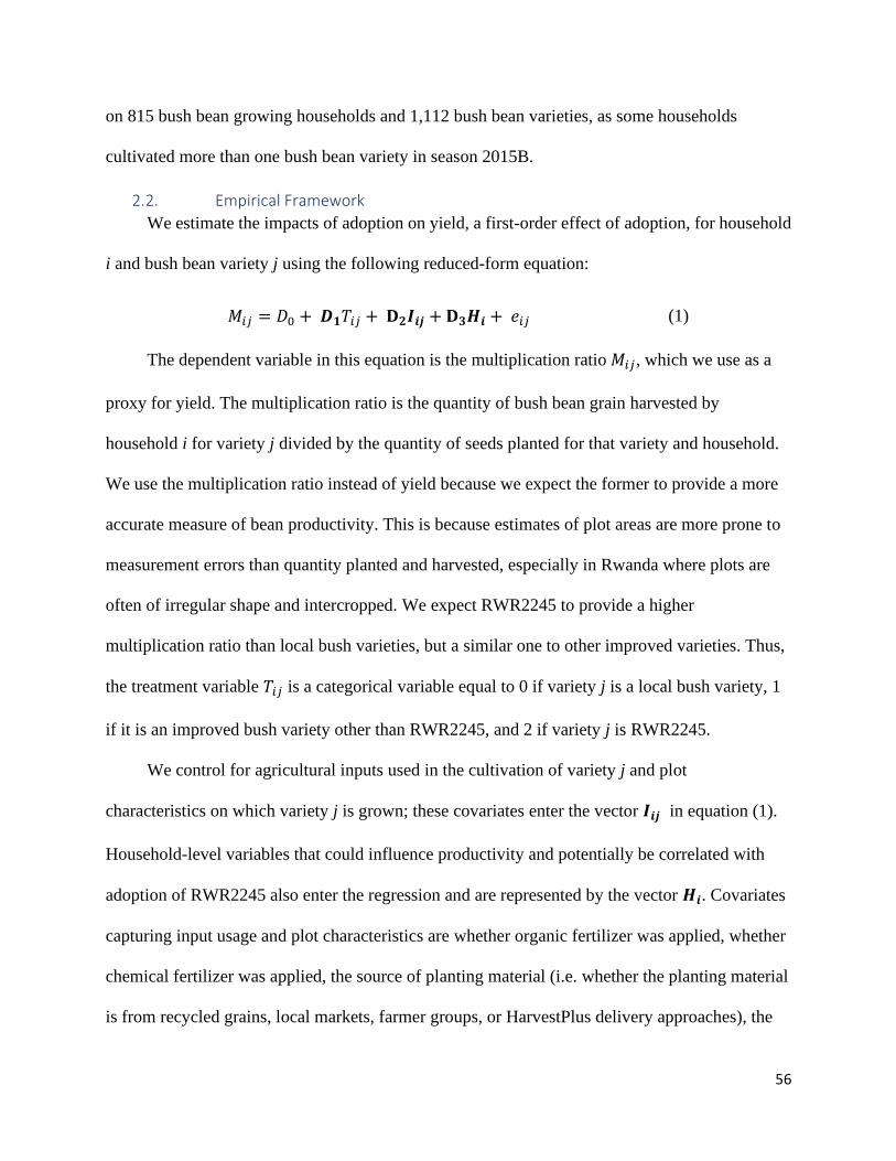
56
on 815 bush bean growing households and 1,112 bush bean varieties, as some households
cultivated more than one bush bean variety in season 2015B.
2.2. Empirical Framework
We estimate the impacts of adoption on yield, a first-order effect of adoption, for household
i and bush bean variety j using the following reduced-form equation:
𝑀𝑖𝑗 = 𝐷0 + 𝑫𝟏𝑇𝑖𝑗 + 𝐃𝟐𝑰𝒊𝒋 + 𝐃𝟑𝑯𝒊 + 𝑒𝑖𝑗 (1)
The dependent variable in this equation is the multiplication ratio 𝑀𝑖𝑗, which we use as a
proxy for yield. The multiplication ratio is the quantity of bush bean grain harvested by
household i for variety j divided by the quantity of seeds planted for that variety and household.
We use the multiplication ratio instead of yield because we expect the former to provide a more
accurate measure of bean productivity. This is because estimates of plot areas are more prone to
measurement errors than quantity planted and harvested, especially in Rwanda where plots are
often of irregular shape and intercropped. We expect RWR2245 to provide a higher
multiplication ratio than local bush varieties, but a similar one to other improved varieties. Thus,
the treatment variable 𝑇𝑖𝑗 is a categorical variable equal to 0 if variety j is a local bush variety, 1
if it is an improved bush variety other than RWR2245, and 2 if variety j is RWR2245.
We control for agricultural inputs used in the cultivation of variety j and plot
characteristics on which variety j is grown; these covariates enter the vector 𝑰𝒊𝒋 in equation (1).
Household-level variables that could influence productivity and potentially be correlated with
adoption of RWR2245 also enter the regression and are represented by the vector 𝑯𝒊. Covariates
capturing input usage and plot characteristics are whether organic fertilizer was applied, whether
chemical fertilizer was applied, the source of planting material (i.e. whether the planting material
is from recycled grains, local markets, farmer groups, or HarvestPlus delivery approaches), the

57
slope of the plot (flat, gentle, moderate, or steep), whether the plot was intercropped, and the
distance from the plot to the household (in minutes walking). The vector 𝑰𝒊 also includes the sex,
literacy, and years of experience growing beans of the household member who makes planting
decisions for the plot on which variety j was grown since the decision maker about bean
production activities varies across plots for household i. The household-level covariates that do
not vary within a household (i.e. those included in vector 𝑯𝒊) are dwelling elevation, the number
of adults in the household as a proxy for farm labor availability, the number of pieces of
agricultural equipment owned, and the percentage of households in the village who obtain advice
from agricultural extension agents, which captures access to extension and is measured at the
village level to avoid endogeneity. Last, we also include province fixed effects to control for
differences in agricultural potential, infrastructure, etc. between provinces.
We estimate the impact of RWR2245 adoption on the higher-order outcomes using the
following equation:
𝑶𝒊 = 𝑓(𝐴𝑖, 𝑯𝒊, 𝑫) + 𝑒𝑖 (2)
where the dependent variable 𝑶𝒊 is the outcome of interest for household i, 𝐴𝑖 is the
treatment variable, and 𝑯𝒊 is a vector of exogenous variables. The vector 𝑶𝒊 includes eight
dependent variables capturing land under bean production, bean consumption from own
production, bean consumption from purchases, and bean sales. We use the quantity of seed
planted in kg as proxy for land area under bean production since it is less prone to measurement
errors than household estimates of land sizes10. We measure bean consumption from own
production using two variables: i) the number of months in the past 12 months prior to data
collection that household i consumed beans from own production and ii) the average monthly
10 Planting density is similar between different bush bean varieties.

58
quantity of beans consumed from own production, measured in kg per adult male equivalent11,
during the months beans were sourced from own production. Adult male equivalents are used to
approximate the food requirements of the household based on the proportional energy
requirements of household members of different gender and age compared to an adult male,
which is the standard reference (Dary and Hainsworth, 2008). Taking into account the food
requirements of different household members provides a more accurate indicator of household
food consumption adequacy than a simpler per-capita measure. Likewise, bean consumption
from purchases are captured using: i) the number of months, in the 12 months prior to data
collection, that the household purchased beans for consumption and ii) the average quantity
purchased per adult equivalent, in kg, during the months beans were consumed from the market.
Indicators representing bean sales are: i) whether household i sells beans, ii) the quantity of
beans sold in the past 12 months, in kg, and iii) whether household i is a net seller of beans,
which is determined by comparing total bean purchases with total bean sales in the past 12
months. Household i is a net seller if total sales exceeded total purchases.
The treatment variable in equation (2) is 𝐴𝑖, a binary treatment variable that measures
adoption and varies by dependent variable. When the dependent variable is land devoted to bean
production, 𝐴𝑖 is equal to one if household i grew RWR2245 in season 2015B and zero
otherwise. For the remaining outcomes of interest, 𝐴𝑖 is equal to one if household i grew
RWR2245 in season 2015A only, in season 2015B only, or in both seasons 2015A and 2015B
and zero otherwise. This approach is used for consistency between the treatment variable and the
11 Adult male equivalents are calculated based on a scale obtained by USAID Dary, O., Hainsworth, M., 2008. The
Food Fortification Formulator: Technical Determination of Fortification Levels and Standards for Mass
Fortification. USAID, Washington, DC.

59
outcomes of interest. The outcomes of interest related to bean consumption and sales cover the
12-month period prior to data collection, which spanned over seasons 2015A and 2015B, so the
treatment variable 𝐴𝑖 takes into account the adoption decision in both seasons. We have no
expectation a priori of the effect of adoption on land devoted to bean cultivation. Households
may wish to increase land under bean cultivation to further take advantage of higher yields, or
may instead reduce land under bean to devote more land to other crops. We hypothesize that
adoption, through higher yield, will increase bean consumption from own production while
reducing consumption of purchased beans by increasing (decreasing) the number of months
households consume beans from own production (purchases) or/and increasing (decreasing) the
average monthly quantity the household consumes from own production (purchases). Last, we
expect adoption to increase the probability that a household sells beans, quantity sold, and the
probability of being a net seller of beans due to RWR2245’s higher yield compared to local
varieties.
We control for household-level covariates, which are represented by the vector 𝑯𝒊 in
equation (2), that could affect the higher-order outcomes of interest 𝑶𝒊. These variables include
distance to the nearest city of 50,000 people (in km) and population density (in
inhabitants/square km) as proxies for proximity to markets, elevation (in meters), the number of
household members, the sex, literacy and age of the respondent, land area cultivated in 2015B (in
hectares), a wealth index12 created using polychoric principal components analysis, the number
of pieces of agricultural equipment owned, livestock ownership measured in tropical livestock
12 This included asset ownership (motorcycle/scooter, bicycle, cell phone, radio, and television) and housing
characteristics (glass windows, access to electricity, outer wall material) and source of drinking water.

60
units13, and access to extension by households in the village. Moreover, we control for whether
household i grew climbing beans in 2015B as climbing beans have higher yields on average than
bush beans and could thus impact bean production, consumption, and sales (Katungi et al, 2018).
Finally, we include province fixed effects as in the yield regression.
There may be household or variety-level factors that are correlated with adoption and the
outcomes of interest in equations (1) and (2) that are not controlled for, such as unobserved
farmer ability or access to resources. As a result, the adoption variables would be correlated with
the error terms, eij and ei, causing the treatment effect estimates to be biased. To address this
problem, we use a CFA.
2.3. Estimation Strategies
We use a CFA to address the endogeneity of adoption as this is more efficient than two-
stage least squares (2SLS) when the endogenous variable is non-linear, and is valid for models
that are nonlinear in parameters (Imbens and Wooldridge, 2007). A CFA is a two-stage
procedure that tests and controls for endogeneity. In the first stage, the treatment variable is
regressed on a set of explanatory variables and IVs. The generalized residuals from this
regression are collected. In the second stage, the outcome variable is regressed on the treatment
variable, other explanatory variables, and the generalized residuals from the first stage
regression. A t-test of the coefficient on the generalized residuals tests the null hypothesis that
the treatment is exogenous (Wooldridge, 2014). A CFA can thus provide additional evidence
beyond the Hausman test as to whether adoption is endogenous to our outcomes of interest and if
so, allow us to estimate causal effects of adoption by controlling for its endogeneity. When the
adoption variable is categorical (Besamusca et al.), we estimate an ordered Probit model in the
13 1 cow = 0.5; 1 sheep = 0.1; 1 goat = 0.1; 1 pig = 0.2; 1 chicken = 0.01; 1 rabbit = 0.02.

61
first stage. When adoption is measured using a binary indicator (Ai), the first stage regression is
estimated using a Probit model.
The second stage estimation methods vary depending on the form of the dependent
outcome variable. When the dependent variable is continuous, as it is for the multiplication ratio,
quantity of bean seeds planted, and average quantity of beans consumed per month when beans
are sourced from own production and purchases, we use ordinary least squares (Kolstad) in the
second stage. We assume a log-linear function because the distribution of these outcomes is
highly skewed to the right.
For quantity sold, we estimate a double hurdle model, also called Craggit (Burke, 2009), in
the second stage because bean sales are censored, with a large number of observations at zero.
Since factors that affect the decision to sell beans may differ from those that influence quantity
sold, it is appropriate to model these two processes separately. The double hurdle model consists
of estimating a probit model in the first stage and a truncated normal regression in the second
stage. Combining the first and second stage estimates, we calculate the average partial effect of
adoption on quantity of beans sold (Burke, 2009). Unlike the Tobit model, the double hurdle
model does not require the explanatory variables to have the same effect on the decision to sell
beans and the quantity sold. We test the double hurdle model against the Tobit model to
determine which model fits the data best.
When the dependent variable is the number of months beans were consumed from own
production, we estimate a Poisson model. For the number of months beans were purchased, we
estimate a zero-inflated Poisson model because some households did not purchase beans over the
past 12 months. Similar to the double hurdle model, the zero-inflated Poisson model allows the
decision to purchase beans to be modeled separately from the number of months beans are

62
purchased. We test whether the zero-inflated Poisson model or the standard Poisson model fit the
data better using a Vuong test. Finally, for the decision to sell beans and whether the household
is a net seller, we estimate Probit models as these are binary outcomes.
Standard errors are robust to heteroscedasticity and clustered at the household level when
the dependent variable is the multiplication ratio since several households cultivate more than
one bush bean variety, resulting in more than one observation per household. For the other
models, standard errors are also robust to heteroscedasticity but clustered at the village level.
Because iron-biofortified bean adopters were oversampled during data collection, we use
sampling weights in all descriptive and econometric analyses.
2.4. Instrumental Variables
CFA requires the inclusion of IVs in the first stage regression. A relevant and valid IV is
one that is correlated with the treatment variable and uncorrelated with the outcome of interest
(Wooldridge, 2010). We use two IVs. The first one is the number of locations where HarvestPlus
sold iron-biofortified bean seeds in local markets in a household’s sector during seasons 2015A
and 2015B. Direct marketing is highly correlated with adoption of biofortified bean varieties
(Vaiknoras et al., 2017). The locations of the direct markets selected for the promotion and sale
of iron-biofortified seed were chosen independently of bean productivity, consumption,
purchases, and sales of local households, which also makes direct marketing exogenous to our
outcomes of interest.
Our second IV is the village adoption rate for RWR2245 in the season prior to the one the
outcome variables are measured. This is a proxy for the availability of RWR2245 planting
material within a household’s social network. The previous season village adoption rate strongly
correlates with current season adoption (Vaiknoras et al., 2017) and is exogenous to an
individual household’s yields, consumption, purchases, and sales in the current season as it is

63
based on other farmers’ previous adoption decisions. Like the treatment variable, the seasons
considered when measuring village adoption rate vary by dependent variable. When the
dependent variables are yield and land under bean production, we use the village adoption rate
for RWR2245 in season 2015A because in these regressions adoption is defined as growing
RWR2245 in 2015B. For the remaining dependent variables, the IV is the village adoption rate
for RWR2245 in season 2014B because adoption is defined over 2015A and 2015B. We test the
validity of the IVs using a series of diagnostic tests for 2SLS regressions (Baum et al., 2002).
2.5. Robustness checks
To test the validity of our results, we implement several robustness checks. We use PSM to
evaluate the treatment effect of adoption on first- and higher-order outcomes. For the
multiplication ratio, we first estimate a logit model to evaluate the propensity score, or the
probability that variety j will be RWR2245, based on observable characteristics in Iij and Hi.
Then propensity scores are used to match multiplication ratios for RWR2245 and local bush bean
varieties that are “similar, i.e. have propensity scores that are close to one another. We compare
RWR2245 only to local bush varieties because we are primarily interested in the yield gain of
RWR2245 over local varieties rather than other improved varieties. For the higher-order
outcomes, we compute the propensity score of a household being an RWR2245 adopter and
compare the outcomes of adopting and non-adopting households that have similar propensity
scores. The final step is to estimate whether these similar varieties (households) have
systematically different outcome values (Austin, 2011).
There are several ways to match control and treatment observations when doing PSM. As a
sensitivity check, we use three common algorithms for matching: nearest neighbor matching,
radius matching, and kernel matching (Caliendo and Kopeinig, 2005). We set a caliper
requirement that matches must have propensity scores that do not differ by more than 0.01. We

64
use the observations in the common support, which is the area where propensity scores between
the treatment and comparison groups overlaps, in order to improve matching (Caliendo and
Kopeinig, 2005).
PSM only explicitly controls for overt bias, meaning that if hidden bias (based on
unobserved characteristics) is present, results will be biased. An advantage of PSM is that it
requires fewer functional form assumptions about the relationship between the outcomes of
interest and explanatory variables, which is why we use it to assess the robustness of our results.
To assess how well PSM controls for overt bias, the balance of matched observations must be
examined as this provides evidence of how comparable the treatment and control groups are
post-matching. One way to do this is to compute the standardized bias, which quantifies the
balance. Harder et al. (2010) consider a covariate to be balanced if its standardized bias is less
than 0.25, although they recommend using a stricter cut-off of 0.10 when possible, particularly
for covariates that are highly correlated with the outcome variable to ensure that the treatment
and control groups are comparable and matching estimates are unbiased14.
For the multiplication ratio regression, we also estimate a fixed effects (FE) model using a
sub-sample of households who grew RWR2245 and at least one other bush bean variety in
2015B. Reducing the sample to partial adopters and using fixed effects eliminates household-
level unobserved heterogeneity, which provides a robustness check for the effects of RWR2245
adoption on productivity. The FE estimator only considers within-household variation and, when
14 We use the user-written Stata commands psmatch2 and pstest to perform PSM and assess post-balance matching,
respectively Leuven, E., Sianesi, B., 2003. PSMATCH2: Stata module to perform full Mahalanobis and propensity
score matching, common support graphing, and covariate imbalance testing:.

65
estimating the effect of growing RWR2245 over a local bush variety, only takes into account
those households that grew both.
Finally, for a subset of outcome variables, i.e. the number of months beans consumed were
from own production and purchased in the market, whether the household sells beans, and
whether it is a net seller, we evaluate the sensitivity of the findings to different measures of
adoption. The alternative measures for adoption are: i) a variable that takes the value of 0, 1, or 2
to reflect the number of seasons in 2015 that a household grew RWR2245, ii) a dummy variable
equal to one if a household adopted RWR2245 in both 2015A and 2015B, iii) a count variable
for the total number of seasons a household has grown RWR2245, conditional on having grown
RWR2245 in 2015, iv) the average percentage of bean land area under RWR2245 between
2015A and 2015B, v) the sum of RWR2245 seeds planted (in kg) in 2015A and 2015B, and vi) a
dummy variable equal to one if a household adopted RWR2245 in any season prior to 2015A but
did not cultivate RWR2245 in 2015. For the last estimation, we expect the adoption variable to
be either insignificant or have a smaller coefficient than variables measuring adoption in 2015
since adoption in prior seasons should not directly affect bean production in 2015.
2.6. Descriptive Statistics
2.6.1. Adoption measures
About 13% of the 1,112 bush bean varieties planted by bush bean growers in 2015B are
RWR2245, 68% are local bush varieties, and 19% are other improved bush varieties, including
the other iron-biofortified bush variety, RWR2154, which makes up less than 1% of the
observations (figure 3-2). Among the 21% of bush bean growers who cultivated RWR2245 in
2015, 4% cultivated RWR2245 in 2015A only, 11% in 2015B only, and 6% in both seasons
(figure 3-3). More than half of the adopters planted RWR2245 for the first time in 2015. Nine
percent of households not growing RWR2245 in 2015 had grown the variety in a previous

66
season. Adoption of RWR2245 varies greatly by province; in 2015, 25% of bush bean growing
households in the East cultivated RWR2245 compared to 22% in the South, 15% in Kigali, 9%
in the West, and 8% in the North.
Figure 3- 2: Bean variety types grown in 2015B
Figure 3- 3: RWR2245 adoption by household in 2015
2.6.2. Outcome variables
The average multiplication ratio is 8.25 for RWR2245, 8.26 for other improved bush bean
varieties, and 6.74 for local bush bean varieties (figure 3-4). The average multiplication ratio for

67
RWR2245 and other improved varieties is significantly higher than that of local varieties. The
multiplication ratio for RWR2245 increases with experience growing the variety: the average
multiplication ratio for first-time adopters is 7.22 compared to 9.15 for those having grown the
variety for more than one season, a difference that is significant at the 10% level. Adopters of
RWR2245 planted 16.32 kg of seeds in 2015B while non-adopters planted 14.14 kg (figure 3-5),
suggesting that adopters have more land planted to beans.
Figure 3- 4: Average multiplication ratio of bush varieties
Note: * = significance at 10%; ** = significance at 5%; *** = significance at 1%

68
Figure 3- 5: Quantity of beans planted in 2015B
Note: * = significance at 10%; ** = significance at 5%; *** = significance at 1%
Households that grew RWR2245 in at least one season in 2015 consumed beans from own
production for 8.59 months on average in the past 12 months, which is 1.3 months (about 40
days) more than non-adopters did (significant at 5%). RWR2245 adopters purchased beans for
about 1.3 months fewer than non-adopters (table 3-1). However, the average quantities
consumed per month did not vary by adoption status. RWR2245 adopters were more likely to
sell beans, sold greater quantities, and were more likely to be net sellers than households that did
not grow RWR2245 in 2015.
Figure 3-6 shows bean consumption trends by month and adoption status from September
2014 to August 2015. Consumption from own production is greatest in January and February,
following season A, and in June and July, which follows season B (Asare-Marfo et al., 2016b).
From March to May and October to November, which are a few months after seasons A and B
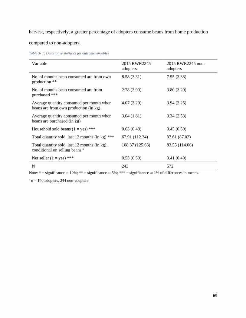
69
harvest, respectively, a greater percentage of adopters consume beans from home production
compared to non-adopters.
Table 3- 1: Descriptive statistics for outcome variables
Variable 2015 RWR2245
adopters
2015 RWR2245 non-
adopters
No. of months bean consumed are from own
production **
8.58 (3.31) 7.55 (3.33)
No. of months bean consumed are from
purchased ***
2.78 (2.99) 3.80 (3.29)
Average quantity consumed per month when
beans are from own production (in kg)
4.07 (2.29) 3.94 (2.25)
Average quantity consumed per month when
beans are purchased (in kg)
3.04 (1.81) 3.34 (2.53)
Household sold beans (1 = yes) *** 0.63 (0.48) 0.45 (0.50)
Total quantity sold, last 12 months (in kg) *** 67.91 (112.34) 37.61 (87.02)
Total quantity sold, last 12 months (in kg),
conditional on selling beans a
108.37 (125.63) 83.55 (114.06)
Net seller (1 = yes) *** 0.55 (0.50) 0.41 (0.49)
N 243 572
Note: * = significance at 10%; ** = significance at 5%; *** = significance at 1% of differences in means.
a n = 140 adopters, 244 non-adopters

70
Figure 3- 6: Consumption and purchases of beans by bush bean growers, by month and RWR2245 adoption status
2.6.3. Explanatory and Instrumental Variables
RWR2245 is less likely to be grown from recycled planting material and more likely to be
grown using organic and chemical fertilizer than local bush bean varieties (table 3-2).
Households who grew RWR2245 in either season of 2015 were less likely to have grown a
climbing bean variety in 2015B than those that did not (table 3-3). RWR2245 adopters were also
more likely to be literate and live in villages with greater access to extension. The remaining
explanatory variables do not statistically differ between plots under RWR2245 and local bush
bean varieties, or between adopters and non-adopters, although the average values for the IVs do
vary. Households that grew RWR2245 were more likely to live in a sector with a direct
marketing approach, although this difference is significant at the 10% level only (table 3-3), and
to live in villages with a greater proportion of RWR2245 adopters in 2014B and 2015A.

71
Table 3- 2: Descriptive statistics of plot-level variables by variety types, season 2015B
RWR2245 Other improved Local bush varieties
Mean (sd) Mean (sd) Mean (sd)
Recycled seed (1 = yes) ** 0.27 (0.45) 0.44 (0.48) 0.39 (0.49)
Slope
Flat 0.10 (0.30) 0.12 (0.32) 0.08 (0.27)
Gentle 0.11 (0.32) 0.16 (0.37) 0.14 (0.35)
Moderate 0.39 (0.49) 0.29 (0.46) 0.35 (0.48)
Steep 0.39 (0.49) 0.43 (0.50) 0.43 (0.49)
Intercrop (1 = yes) 0.60 (0.49) 0.51 (0.50) 0.66 (0.48)
Walking time to househ (in minutes) 18.18 (33.07) 22.20 (31.09) 15.58 (23.07)
Organic fertilizer use (1 = yes) ** 0.83 (0.37) 0.71 (0.46) 0.71 (0.45)
Chemical fertilizer use (1 = yes) ** 0.17 (0.38) 0.12 (0.33) 0.07 (0.27)
Sex of plot decider (1= female) 0.59 (0.49) 0.61 (0.49) 0.61 (0.49)
Literacy of plot decider (1=yes) 0.65 (0.48) 0.59 (0.49) 0.59 (0.49)
Experience of plot worker (in years) 25.92 (14.19) 26.60 (15.40) 27.50 (16.70)
211 222 679 Note: * = significance at 10%; ** = significance at 5%; *** = significance at 1% of differences in means.
Table 3- 3: Descriptive statistics of household-level variables by RWR2245 adoption status in 2015
RWR2245 growers RWR2245 non-growers
Variables Mean (sd)
or % yes
Mean (sd)
or % yes
Climbing bean grower (1 = yes) *** 0.18 (0.38) 0.27 (0.45)
Distance to city (km) 36.51 (21.62) 36.09 (23.13)
Population density (people/square km) 484.68 (537.21) 452.54 (453.35)
Elevation (10m) 156.58 (15.69) 159.16 (19.86)
Household size 4.92 (2.06) 4.87 (1.99)
Sex of bean decision maker (1 = female) 0.62 (0.49) 0.64 (0.48)
Literacy of bean decision maker (1 = yes) ** 0.69 (0.46) 0.59 (0.49)
Age of bean decision maker (in years) 44.44 (13.74) 43.84 (15.43)
Land size (ha) 0.54 (0.70) 0.50 (0.75)
Wealth
1 0.18 (0.39) 0.23 (0.40)
2 0.16 (0.37) 0.19 (0.41)
3 0.17 (0.38) 0.20 (0.40)
4 0.20 (0.41) 0.18 (0.40)
5 * 0.28 (0.45) 0.20 (0.39)
Equipment owned (count) * 1.38 (0.75) 1.21 (0.79)
Livestock (TLU) 0.54 (0.88) 0.46 (1.15)
Extension (%) ** 65.59 (24.61) 62.06 (25.48)
Direct markets 2015A and 2015B (#) * 0.47 (1.67) 0.26 (1.05)
Village RWR2245 adoption rate 2014B (%) *** 0.11 (0.10) 0.06 (0.08)
Village RWR2245 adoption rate 2015A (%) *** 0.18 (0.15) 0.10 (0.10)
243 572 Note: * = significance at 10%; ** = significance at 5%; *** = significance at 1% of difference in means.

72
To provide evidence that HarvestPlus did not deliberately target areas with greater bean
productivity, consumption, or marketing for the dissemination and promotion of iron-biofortified
beans, we compare households who live in sectors where direct marketing took place in 2015
with those that did not. If the outcomes of interest and explanatory variables do not differ with
household proximity to direct marketing, then this provides evidence that direct marketing is a
valid IV. The average multiplication ratio does not differ between households who live in sectors
with a direct marketing approach in 2015 and those that do not live in such sectors. In addition,
none of our higher order household-level outcome variables vary significantly by whether the
household has a direct marketing approach in its sector.
The prevalence of direct marketing approaches varies by provinces; in 2015, 22% of bush
bean growing households in the Northern province had a direct marketing approach in their
sector compared to 23% in the West, 21% in the East, 3% in the South, and none in Kigali.
Households in sectors where direct marketing took place live farther from cities (44.11 km vs.
34.80 km) and in villages where a higher percentage of farmers obtain information from
extension (77.43% vs. 60.26%) compared to households who did not have direct marketing in
their sector. Other household characteristics, including literacy, wealth, and land under
cultivation, do not vary by whether the households had direct marketing in their sector. This
lends support that data on formal delivery approaches can provide a valid IV for RWR2245
adoption.

73
3. Results
3.1. Instrument validity, endogeneity tests, and model fit
Diagnostic tests provide evidence that the IVs are valid (table 4). We reject the null
hypothesis that the model is underidentified based on a Kleibergen-Paap rk LM statistic test. The
null hypothesis of weak IVs is rejected for each outcome using the Cragg-Donald F statistic. In
all models, the Hansen J test for overidentification fails to reject the null hypothesis that the IVs
are valid, indicating that the IVs are not correlated with the error term and correctly excluded
from the outcome regressions. The Hausman test fails to reject the null hypothesis that adoption
is exogenous in all models, suggesting that adoption is not endogenous to our outcomes of
interest.
In the productivity regression, the coefficient for the generalized residuals is statistically
significant (table 3-5), indicating that adoption is endogenous to the multiplication ratio
(Wooldridge, 2014). In all remaining regressions, the p-value of the coefficient for the
generalized residuals ranges from 0.356-0.892 which is consistent with the Hausman test that
adoption is exogenous. In that case, the non-CFA estimation results are equally valid as the CFA
results, and likely more efficient (Wooldridge, 2014). Therefore, for these models, we discuss the
results for which adoption is considered exogenous.

74
Table 3- 4: Instrument diagnostic test results for multiplication ratio, consumption, purchases, and sales
Yield Log
beans
planted
Months
consumed
Log
quantity
consumed
Months
purchased
Log
quantity
purchased
Total
Sales
Underidentification test
Kleibergen-Paap rk LM
statistic
25.509 31.833 22.415 23.146 22.415 13.023 22.415
Chi-sq (2) P-val 0.000 0.000 0.000 0.000 0.000 0.002 0.000
Weak identification test
Cragg-Donald Wald F
statistic
16.726 31.004 20.236 20.838 20.236 12.337 20.236
Sanderson-Windmeijer
test p-value
0.000 0.000 0.000 0.000 0.000 0.000 0.000
Overidentification test
Hansen J statistic 1.802 0.404 1.263 0.480 1.595 0.036 2.035
Chi-sq (1) P-val 0.179 0.525 0.261 0.489 0.201 0.850 0.154
Endogeneity test
Hausman test statistic 2.133 0.008 0.066 0.103 0.047 0.001 0.021
Chi-sq (1) P-val 0.144 0.928 0.797 0.749 0.829 0.978 0.886
Based on a likelihood ratio test, the restrictions that the Tobit model holds are rejected (p =
0.000), confirming that the double hurdle model is a better fit than the Tobit model for
explaining quantity sold. The Vuong test also confirms that the zero-inflated Poisson fits the data
for the number of months beans were purchased better than the standard Poisson (p = 0.000)
(Desmarais and Harden, 2013). After performing PSM, the standardized bias for all covariates is
less than 25%, and below 10% for most covariates, which is within recommended limits,
indicating that our matching procedures do an adequate job at balancing treatment and control
groups and thus controlling for overt bias of the adoption decision (Harder et al., 2010). To
achieve this balance for the multiplication ratio regression using nearest neighbor matching, we
had to use two control matches for each treatment observation; otherwise, the use of chemical
fertilizer did not meet the 25% cut-off value (its standardized bias is 27% when one match is
used).

75
3.2. Supply indicator results
Holding other factors constant, the multiplication ratio for RWR2245 is 49% (100*(e.398 -
1)) higher than that local bush varieties according to CFA estimates, and the coefficient is
significant at the 1% level (table 3-5). In the FE model, the treatment effect of adoption indicates
a 20% yield increase over local bush bean varieties, statistically significant at the 5% level, for
households that grow both RWR2245 and a local variety. Other improved varieties provide a
yield gain of about 23% and 37% over local varieties according to the CFA estimates and FE (for
households that grow both an improved and a local variety) results, respectively. PSM indicates
that the multiplication ratio for RWR2245 is 23-26% higher than for local bush bean varieties
(table 3-7). Being grown from recycled grain, the literacy of the plot decision maker, ownership
of agricultural equipment, and access to extension have a positive effect on the multiplication
ratio. In the reduced sample, growing beans on a flat or gentle slope and applying chemical
fertilizer both increase the multiplication ratio.
The average multiplication ratio for local varieties is 6.74, meaning that a 49% yield gain
would correspond to a multiplication ratio of 9.44. On average, bush bean growers planted 15.57
kg of bush bean seed in 2015B; if this seed were entirely local bush varieties, the average
household would harvest 104.94 kg of beans. Converting all planted bush bean seed from local
bush varieties to RWR2245 would provide a harvest of 156.32 kg, which corresponds to an
additional 51.38 kg of beans per season compared to no adoption of improved varieties. When
excluding RWR2245, 78% of bush bean varieties grown in 2015B were local varieties and 22%
were other improved varieties. Taking this into account, and assuming no difference in
multiplication ratio between RWR2245 and other improved varieties, the average harvest gain
from RWR2245 adoption is 40.08 kg per season, or about 80 kg per year.

76
Adoption of RWR2245 has no effect on the quantity of bean seed planted (tables 3-6 and
3-7), suggesting that adoption does not lead to changes in the proportion of land devoted to bean
cultivation. Adopters therefore obtain higher quantities of harvested grain as a result of adoption.
This extra production can lead to higher-order outcomes such as greater quantity consumed
and/or sold, and likely an improvement in household nutrition. Households that live farther from
cities, have more household members, cultivate more land, own more livestock, and are
wealthier have more land under bean cultivation while households at higher elevations have less
land devoted to beans.

77
Table 3- 5: Regression results for multiplication ratio
Multiplication ratio (quantity harvested/quantity planted)
OLS Coefficient
(Robust std. err.)
CFA OLS Coefficient
(Robust std. err.)
FE Coefficient
(Robust std. err.)
Adjusted R2 0.113 0.122
R2 within
0.145
R2 between
0.002
R2 overall
0.001
Type (base = local)
Other improved 0.189** 0.207** 0.312**
(0.081) (0.080) (0.137)
RWR2245 0.183** 0.398*** 0.182**
(0.082) (0.088) (0.087)
Recycled seed (1 = yes) 0.235*** 0.233*** 0.191 (0.062) (0.061) (0.121)
Slope (base = steep) Moderate 0.138 0.150 0.323 (0.138) (0.136) (0.263)
Gentle 0.044 0.052 0.534** (0.130) (0.129) (0.266)
Flat 0.145 0.161 0.956*** (0.128) (0.127) (0.226)
Intercrop (1 = yes) -0.111 -0.096 0.269 (0.068) (0.067) (0.214)
Walk time to house (in minutes) -0.003* -0.003* 0.001
(0.002) (0.002) (0.003)
Organic fertilizer use (1 = yes) -0.097 -0.120 -0.243 (0.082) (0.080) (0.252)
Chemical fertilizer use (1 = yes) 0.087 0.068 0.502** (0.113) (0.113) (0.236)
Sex (1 = female) -0.051 -0.059 0.150 (0.072) (0.071) (0.362)
Literate (1 = yes) 0.271*** 0.272*** -0.742 (0.078) (0.078) (0.771)
Experience (in years) 0.001 0.001 -0.076 (0.002) (0.002) (0.105)
Elevation (10m) -0.001 -0.001 (0.002) (0.002) Number of adults 0.004 0.003 (0.028) (0.028) Equipment owned (count) 0.107** 0.107** (0.045) (0.045) Extension (%) 0.005*** 0.005*** (0.002) (0.002) Generalized residual -0.057***
(0.007) Constant 0.988* 1.029** 3.168 (0.386) (0.381) (2.199)
N 1112 1112 336
Note: * = significance at 10%; ** = significance at 5%; *** = significance at 1%. Standard errors are robust to
heteroskedasticity for all models and clustered at the household level for OLS and CFA OLS models. Coefficients
for province fixed effects are not shown for brevity.

78
Table 3- 6: Regression results for log of total kg of beans planted in season 2015B
Log of total kg beans planted 2015B
OLS Coefficient (Robust std. err.) CFA OLS Coefficient (Robust std. err.)
Adj. R2/Pseudo R2 0.254 0.253
Adopted 2015 (1 = yes) 0.079 0.168 (0.077) (0.269)
Climbing bean grower (1 = yes) 0.287*** 0.290*** (0.068) (0.068)
Distance to city (km) 0.008*** 0.008*** (0.003) (0.003)
Population density (people/square
km)
0.000 0.000
(0.000) (0.000)
Elevation (10m) -0.009*** -0.009*** (0.002) (0.002)
Household size 0.022 0.022 (0.017) (0.017)
Sex (1 = female) -0.101 -0.101 (0.063) (0.063)
Literate (1 = yes) 0.044 0.039 (0.073) (0.073)
Age (in years) 0.003 0.003 (0.002) (0.002)
Land size (ha) 0.232*** 0.232*** (0.086) (0.086)
Wealth (base = 1) 0.000 0.000
2 0.026 0.022 (0.096) (0.096)
3 0.103 0.101 (0.108) (0.109)
4 0.330*** 0.325*** (0.117) (0.117)
5 0.261** 0.254** (0.109) (0.116)
Equipment owned (count) 0.022 0.023 (0.047) (0.047)
Livestock (TLU) 0.086*** 0.086*** (0.017) (0.017)
Extension (%) -0.004*** -0.004*** (0.001) (0.001)
Generalized residual -0.054
(0.147)
Constant 3.267*** 3.261*** (0.448) (0.448)
N 815 815
Note: * = significance at 10%; ** = significance at 5%; *** = significance at 1%. Standard errors are robust to
heteroskedasticity for all models and clustered at the village level. Coefficients for province fixed effects are not
shown for brevity.

79
Table 3- 7: Matching results for supply indicators
Matching algorithm Yield Beans planted
Nearest Neighbor 0.262 (0.094) *** 0.053 (0.123)
Radius 0.232 (0.075) *** 0.074 (0.068)
Kernel 0.228 (0.069) *** 0.083 (0.075)
N 890 815
Note: Standard errors are bootstrapped. Caliper is set to 0.01 for all matching algorithms.
3.3. Consumption indicator results
RWR2245 adoption (season 2015A, B or both) increases bean consumption from home
production by 0.64 months (equivalent to 19-20 days) (table 3-8) while reducing the length of
time beans have to be purchased by 0.73 months (equivalent to 22-23 days) in a year (table 3-9).
However, adoption of RWR2245 has no effect on the average quantity consumed monthly when
beans are sourced from own production or the market (table 3-8 and 3-9). This suggests that
adoption does not change quantity consumed, but changes the source of beans consumed,
moving away from purchases towards own production. As an additional robustness check, we
estimated a regression with the log of the sum of bean consumed from own production and
purchases as the dependent variable. We find no effect of RWR2245 adoption on the total
quantity of beans consumed in the last 12 months.
Adopting RWR2245 increases the probability of selling beans by 12% and increases the
quantity of beans sold by 17.28 kg, although the effect on quantity sold is significant at the 10%
level only (table 3-10). RWR2245 adopters are also 8% more likely to be net sellers of beans,
with the coefficient being significant at the 10% level. The low levels or lack of significance of
adoption on quantities consumed, purchased, and sold could be partially due to difficulties for
the respondents to recall and correctly estimate these quantities over a 12-month period.
However, it should be easier to remember when the household consumed beans from own
production and purchase and whether they sold beans. This may also affect the precision and

80
magnitude of our estimate of the impact of adoption on the likelihood of being a net seller of
beans.
Climbing bean growers consume beans from own production for more months than those
that grow bush beans only, which is not surprising given the yield advantage of climbers over
bush beans and is consistent with previous findings (Katungi et al., 2018). Distance from an
urban area has a positive effect on the number of month beans are consumed from own
production, selling and being a net seller, and a negative effect on the number of months beans
are purchased. Population density and elevation have a negative effect on the number of months
beans are consumed from own production but a positive effect on the number of months a
household purchases beans. Households at higher elevation are also less likely to sell beans or be
net sellers of beans. Household size has a positive effect on the number of months beans are
purchased, but a negative effect on the average quantity purchased per month, the number of
months beans are consumed from own production, and being a net seller of beans. Literacy of the
respondent has a negative effect on the number of months beans are purchased but a positive
influence on the average monthly quantity consumed from purchases and own production. The
age of the respondent increases the number of months beans are consumed from own production
while reducing the number of months beans are purchased. Households that cultivate more land
consume beans from own production for a greater number of months, purchase beans for fewer
months, sell higher quantities of beans, and are more likely to be net sellers of beans. The wealth
index and the number of pieces of agricultural equipment owned have a positive effect on the
number of months households consume beans from own production and a negative effect on the
number of months beans are purchased. The wealth index also has a negative impact on the
average monthly quantity consumed from own production while agricultural equipment

81
ownership has a positive effect on the average monthly quantity purchased. Livestock ownership
has a positive effect on the average monthly quantity consumed from own production but a
negative influence on the number of months a household purchase beans. Finally, access to
agricultural extension makes households more likely to sell beans.

82
Table 3- 8: Regression results for number of months households consume beans from own production and average monthly
quantity consumed from own production
Months consumed from own production Quantity (kg) consumed each
month, per adult equivalent
Poisson marginal
effects (Delta
method Std. Err.)
CFA Poisson
marginal effects
(Delta method Std.
Err.)
OLS coefficient
(robust Std.
Err.)
CFA OLS
coefficient
(robust Std. Err.)
Adj. R2
0.107 0.107
Log psuedolikelihood -2427222.7 -2426875.1
Adopted 2015 (1 = yes) 0.641** 1.392 0.012 0.079
(0.287) (1.234) (0.057) (0.235)
Climbing bean grower (1 =
yes)
0.752** 0.795*** -0.033 -0.029
(0.291) (0.294) (0.054) (0.054)
Distance to city (km) 0.026*** 0.027*** 0.000 0.000 (0.009) (0.011) (0.002) (0.002)
Population density
(people/square km)
-0.001*** -0.001*** 0.000 0.000
(0.000) (0.000) (0.000) (0.000)
Elevation (10m) -0.021*** -0.020*** -0.001 -0.001 (0.007) (0.007) (0.001) (0.001)
Household size -0.144** -0.144** -0.094*** -0.094*** (0.070) (0.071) (0.011) (0.011)
Sex (1 = female) -0.368 -0.376 -0.064 -0.065 (0.272) (0.268) (0.049) (0.048)
Literate (1 = yes) 0.571* 0.518* 0.178*** 0.174*** (0.303) (0.299) (0.059) (0.063)
Age (years) 0.026*** 0.032*** 0.001 0.001 (0.007) (0.010) (0.001) (0.001)
Land size (ha) 0.613*** 0.616*** 0.046 0.046 (0.125) (0.124) (0.032) (0.032)
Wealth quintile (base = 1)
2 0.140 0.128 0.062 0.061
(0.450) (0.453) (0.079) (0.079)
3 0.237 0.236 0.020 0.020 (0.469) (0.470) (0.077) (0.077)
4 0.947** 0.913** -0.024 -0.027 (0.434) (0.442) (0.068) (0.069)
5 1.761*** 1.701*** -0.171** -0.176** (0.473) (0.496) (0.077) (0.075)
Equipment owned (count) 0.636*** 0.592*** 0.027 0.024 (0.138) (0.156) (0.025) (0.032)
Livestock (TLU) 0.067 0.075 0.069*** 0.069*** (0.077) (0.078) (0.012) (0.013)
Extension (%) 0.005 0.004 -0.001 -0.001 (0.005) (0.005) (0.001) (0.001)
Generalized residual
-0.458 -0.040 (0.719) (0.144)
Constant (coefficient) 2.028*** 2.020*** 1.736*** 1.731*** (0.182) (0.183) (0.227) (0.233)
N 815 815 804a 804
Note: * = significance at 10%; ** = significance at 5%; *** = significance at 1%. Standard errors are robust to
heteroskedasticity and clustered at the village level. Coefficients for province fixed effects are not shown for brevity.
a Eleven households did not consume beans from own production in any months

83
Table 3- 9: Regression results for number of months households consume beans from purchases and average monthly quantity
purchased
Months purchased Quantity (kg) purchased each
month, per adult equivalent
Zero-inflated
Poisson marginal
effects (Delta
method Std. Err.)
CFA Zero-inflated
Poisson marginal
effects (Delta method
Std. Err.)
OLS
coefficient
(robust Std.
Err.)
CFA OLS
coefficient
(robust Std.
Err.)
Adj. R2/Pseudo R2 0.175 0.174
Log psuedolikelihood -1995457 -1994473
Adopted 2015 (1 = yes) -0.728*** -0.876 -0.102 -0.171 (0.263) (1.141) (0.071) (0.305)
Climbing bean grower (1 =
yes)
-0.270 -0.271 -0.060 -0.063
(0.275) (0.280) (0.067) (0.069)
Distance to city (km) -0.019** -0.019* 0.001 0.001 (0.009) (0.010) (0.002) (0.002)
Population density
(people/square km)
0.001*** 0.001*** -0.000 -0.000
(0.000) (0.000) (0.000) (0.000)
Elevation (10m) 0.013** 0.013** -0.000 -0.000 (0.006) (0.006) (0.002) (0.002)
Household size 0.187*** 0.187*** -0.103*** -0.103*** (0.055) (0.055) (0.015) (0.015)
Sex (1 = female) 0.142 0.139 -0.010 -0.010 (0.276) (0.276) (0.064) (0.064)
Literate (1 = yes) -0.492** -0.482** 0.177** 0.181** (0.229) (0.238) (0.075) (0.074)
Age (years) -0.031*** -0.031*** 0.003 0.003 (0.008) (0.008) (0.002) (0.002)
Land size (ha) -0.460*** -0.457*** 0.068 0.068 (0.172) (0.172) (0.044) (0.044)
Wealth quintile (base = 1)
2 0.189 0.197 0.106 0.107
(0.365) (0.365) (0.086) (0.085)
3 -0.025 -0.031 0.078 0.078 (0.398) (0.397) (0.098) (0.098)
4 -0.630* -0.630* -0.060 -0.057 (0.368) (0.372) (0.091) (0.094)
5 -1.359*** -1.374*** -0.006 -0.001 (0.395) (0.423) (0.094) (0.095)
Equipment owned (count) -0.517*** -0.511*** 0.125*** 0.128** (0.175) (0.185) (0.045) (0.049)
Livestock (TLU) -0.893*** -0.889*** -0.075 -0.074 (0.284) (0.285) (0.075) (0.074)
Extension (%) 0.006 0.006 -0.003* -0.003* (0.005) (0.005) (0.002) (0.002)
Generalized residual
0.085 0.042 (0.664) (0.177)
Constant 1.861*** 1.795*** 1.283*** 1.291*** (0.973) (0.969) (0.332) (0.335)
N 815 815 562 562
Note: * = significance at 10%; ** = significance at 5%; *** = significance at 1%. Standard errors are robust to
heteroskedasticity and clustered at the village level. Coefficients for province fixed effects are not shown for brevity.

84
Table 3- 10: Regression results for sales and net seller
Sold beans Quantity sold Net seller
Probit
marginal
effects
(Delta
method Std.
Err.)
CFA
Probit
marginal
effects
(Delta
method
Std. Err.)
Double
hurdle
average
partial
effects
(Bootstrappe
d std. err.)
CFA Double
hurdle
average
partial
effects
(Bootstrappe
d std. err.)
Probit
marginal
effects
(Delta
method
Std. Err.)
CFA
Probit
marginal
effects
(Delta
method
Std. Err.)
Adj. R2/Pseudo R2 0.147 0.147 0.192 0.193
Log psuedolikelihood -562430.16 -562421.25 -3047935.5 -3047091.6 -852005.65 -526694.95
Adopted 2015 (1 = yes) 0.122*** 0.103 17.276* 49.202 0.081* 0.005 (0.047) (0.145) (9.081) (40.400) (0.047) (0.139)
Climbing bean grower
(1 = yes)
0.024 0.023 -2.991 -1.062 0.068 0.064
(0.044) (0.045) (9.503) (10.872) (0.043) (0.044)
Distance to city (km) 0.004*** 0.004*** 1.284*** 1.324*** 0.005*** 0.005*** (0.001) (0.001) (0.339) (0.334) (0.001) (0.001)
Population density
(people/square km)
-0.000* -0.000* -0.006 -0.004 -0.000** -0.000**
(0.000) (0.000) (0.011) (0.011) (0.000) (0.000)
Elevation (10m) -0.005*** -0.005*** -0.732*** -0.672*** -0.003*** -0.003*** (0.001) (0.001) (0.268) (0.258) (0.001) (0.001)
Household size -0.004 -0.004 0.184 -0.131 -0.031*** -0.031*** (0.010) (0.010) (2.030) (2.084) (0.010) (0.010)
Sex (1 = female) -0.043 -0.042 -17.436* -18.132* -0.017 -0.016 (0.042) (0.042) (9.129) (10.741) (0.043) (0.043)
Literate (1 = yes) 0.022 0.024 20.276* 17.425* 0.005 0.010 (0.043) (0.044) (10.476) (9.169) (0.044) (0.043)
Age (years) -0.002 -0.002 -0.287 -0.316 0.002* 0.002* (0.001) (0.001) (0.296) (0.288) (0.001) (0.001)
Land size (ha) 0.043 0.043 14.609** 14.475*** 0.070** 0.070* (0.033) (0.033) (6.215) (5.313) (0.036) (0.036)
Wealth quintile (base = 1)
2 0.013 0.014 -16.766 -16.698 -0.031 -0.030 (0.053) (0.053) (23.452) (22.319) (0.052) (0.052)
3 -0.006 -0.006 -0.239 -0.550 0.014 0.014 (0.064) (0.064) (13.040) (13.798) (0.055) (0.054)
4 0.099 0.100 10.911 8.829 0.115** 0.118** (0.068) (0.068) (15.038) (15.189) (0.055) (0.056)
5 0.109 0.110 27.996 25.433 0.254*** 0.260*** (0.072) (0.072) (17.186) (16.682) (0.064) (0.067)
Equipment owned
(count)
-0.022 -0.021 7.881 5.415 0.062** 0.066**
(0.027) (0.029) (5.437) (5.943) (0.030) (0.030)
Livestock (TLU) -0.033 -0.033 -0.634 -0.528 0.118*** 0.119*** (0.028) (0.028) (5.066) (6.569) (0.042) (0.042)
Extension (%) 0.001** 0.001** 0.076 0.029 0.000 0.000 (0.000) (0.000) (0.161) (0.169) (0.000) (0.001)
Generalized residual
0.012 -19.754
0.046 (0.086) (19.017)
(0.077)
Constant (coefficient) 2.120*** 2.126*** -1319.285 -1521.003 0.429 0.453 (0.616) (0.608) (1433.048) (1522.696) (0.540) (0.534)
N 815 815 815 815 815 815
Note: * = significance at 10%; ** = significance at 5%; *** = significance at 1%. Standard errors are robust to
heteroskedasticity and clustered at the village level. Coefficients for province fixed effects are not shown for brevity.

85
The results of PSM analysis are consistent with the previous findings, providing evidence of
the robustness of our results to econometric methods. According to PSM results, adoption of
RWR2245 increases the number of months households consume beans from own production by
0.62-0.64 months, reduces the number of months households purchase beans by 0.66-0.69
months, increases the likelihood of selling beans by 12-14% and the probability of being a net
seller of beans by 9-12% and finally, increases bean sales by an additional 18 to 21 kg per year.
Table 3- 11: Matching results for consumption indicators
Matching
algorithm
Months
consumed
from own
production
Kg
consume
d
Months
purchased
Kg
purchased
Sold beans Kg sold Net seller
Nearest
Neighbor
0.711
(0.390)*
0.101
(0.077)
-0.924
(0.374)**
0.075
(0.084)
0.142
(0.058)**
15.844
(10.584)
0.124
(0.053)**
Radius 0.621
(0.269)**
0.029
(0.047)
-0.662
(0.243)***
-0.051
(0.068)
0.120
(0.042)***
18.409
(8.834)**
0.093
(0.039)**
Kernel 0.644
(0.249)**
0.032
(0.046)
-0.686
(0.229)***
-0.061
(0.057)
0.129
(0.040)***
20.675
(8.102)**
0.101
(0.037)***
N 815 804 815 562 815 815 815
Note: Standard errors are bootstrapped. Caliper is set to 0.01 for all matching algorithms, and only observations that
fall under common support are included.
Alternative specifications of adoption also provide consistent results, providing further
indication that our results are highly robust not only to different estimation methods, but also to
different measures of adoption (table 3-12). If adoption is defined as a count variable equal to the
number of seasons in 2015 that a household grew RWR2245 (0, 1, or 2), results of the Poisson,
zero-inflated Poisson, and probit regressions, respectively, indicate that growing RWR2245 for
an additional season increases consumption from own production by 0.55 months, reduces the
number of months beans are purchased by 0.64 months, and increases the probability of selling
beans and being a net seller by 11% and 8%, respectively (each significant at the 5% level or
lower). If we consider as adopters only households that grew RWR2245 in both seasons of 2015,
adoption increases beans consumption from own production by 1.21 months, reduces bean

86
purchases by 1.39 months, and increases the probability of selling beans and being a net seller by
19% and 21%, respectively, roughly doubling the estimated effects of growing RWR2245 for
one season. Increasing the proportion of bean land under RWR2245 by 10% increases
(decreases) bean consumption from own production (purchases) by 0.02 months (about half a
day) and increases the probability of selling beans and being a net seller of beans by 0.2%.
Planting an additional kg of RWR2245 seeds in 2015A or 2015B increases consumption from
own production by 0.02 months (0.6 days) and increases the probability of selling beans and
being a net seller by 1% each. Conditional on having planted RWR2245 in 2015A or 2015B,
growing RWR2245 an additional season prior to 2015 increases bean consumption from own
production by 0.18 months, reduces the need to purchase beans by 0.26 months, and increases
the probability of being a net seller by 3%, meaning that the benefits of RWR2245 adoption
increases as households get more experience growing the variety. Finally, having grown
RWR2245 prior to 2015A, but not being an adopter in 2015, does not have a significant impact
on the number months beans are consumed from own production and purchases or on the
probability of being a net seller of beans, although it does increase the likelihood of selling beans
by 12%. Thus, regardless of how adoption is measured, results indicate that adopters replace
bean purchases with beans from own production and generate surplus to sell.
When beans are consumed from own production, monthly consumption averages 12.99 kg.
Increasing bean consumption from own production by 1.21 months would therefore require an
additional 15.98 kg of beans harvested over seasons 2015A and 2015B. This is well within reach
given the estimated yield gains of 80 kg over two seasons from converting local bush bean
varieties to RWR2245 and adopters would also have a surplus to sell. Adoption should thus
improve household nutrition through the consumption of beans high in iron content. It should
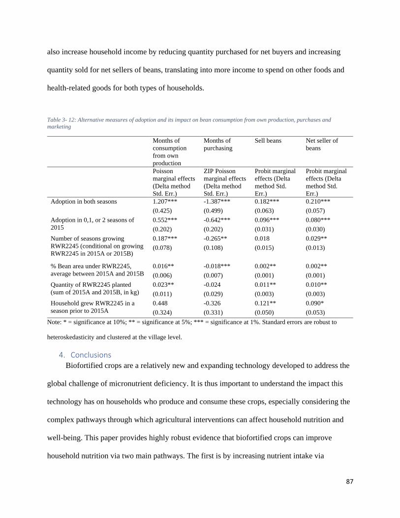
87
also increase household income by reducing quantity purchased for net buyers and increasing
quantity sold for net sellers of beans, translating into more income to spend on other foods and
health-related goods for both types of households.
Table 3- 12: Alternative measures of adoption and its impact on bean consumption from own production, purchases and
marketing
Months of
consumption
from own
production
Months of
purchasing
Sell beans Net seller of
beans
Poisson
marginal effects
(Delta method
Std. Err.)
ZIP Poisson
marginal effects
(Delta method
Std. Err.)
Probit marginal
effects (Delta
method Std.
Err.)
Probit marginal
effects (Delta
method Std.
Err.)
Adoption in both seasons 1.207*** -1.387*** 0.182*** 0.210***
(0.425) (0.499) (0.063) (0.057)
Adoption in 0,1, or 2 seasons of
2015
0.552*** -0.642*** 0.096*** 0.080***
(0.202) (0.202) (0.031) (0.030)
Number of seasons growing
RWR2245 (conditional on growing
RWR2245 in 2015A or 2015B)
0.187*** -0.265** 0.018 0.029**
(0.078) (0.108) (0.015) (0.013)
% Bean area under RWR2245,
average between 2015A and 2015B
0.016** -0.018*** 0.002** 0.002**
(0.006) (0.007) (0.001) (0.001)
Quantity of RWR2245 planted
(sum of 2015A and 2015B, in kg)
0.023** -0.024 0.011** 0.010**
(0.011) (0.029) (0.003) (0.003)
Household grew RWR2245 in a
season prior to 2015A
0.448 -0.326 0.121** 0.090*
(0.324) (0.331) (0.050) (0.053)
Note: * = significance at 10%; ** = significance at 5%; *** = significance at 1%. Standard errors are robust to
heteroskedasticity and clustered at the village level.
4. Conclusions Biofortified crops are a relatively new and expanding technology developed to address the
global challenge of micronutrient deficiency. It is thus important to understand the impact this
technology has on households who produce and consume these crops, especially considering the
complex pathways through which agricultural interventions can affect household nutrition and
well-being. This paper provides highly robust evidence that biofortified crops can improve
household nutrition via two main pathways. The first is by increasing nutrient intake via

88
increased consumption of the own produced biofortified crop. The second pathway occurs by
increasing household income available for the purchase of other nutritious foods via reductions
in purchases and increased sales of the targeted crop. These benefits arise from the enhanced
nutritive value of the biofortified crops and their high-yielding properties which boost harvested
quantity.
More specifically, we find that adoption of the most popular iron-biofortified bean variety,
RWR2245, increases yields by 20-49% over traditional bush bean varieties in Rwanda; this
range of estimates from different estimation methods likely provides a lower and upper bound of
the yield effect. This productivity advantage is crucial for sustained adoption of RWR2245 and a
critical determinant of overall impacts. Having rigorously quantified the productivity gain
strengthens the attribution of the higher-order impacts to the adoption of RWR2245. Households
who grow RWR2245 in one or two seasons consume beans from own production for an
additional 0.62-0.64 months (about 19-20 days) per year compared to those that did not grow
RWR2245. RWR2245 adoption also reduces the need to purchase beans by 0.66-0.92 months
(about 20-28 days) over a 12-month period. Adoption does not change total quantity consumed,
but rather allows households to shift the source of bean consumption away from purchases
toward own production. In addition, adoption increases the likelihood that a household sells
beans by 12-14%. The results are robust to a variety of estimation methods and specifications for
the adoption decision, which provides a high level of confidence in our findings.
Women aged 19-50 need to consume about 18 mg of iron per day (Institute of Medicine,
2018). For an average household, switching all beans consumed from own production from non-
biofortified to biofortified would lead to a substantial increase in iron intake. Glahn et al. (2017)
estimate that one kg of non-biofortified beans contains 47.5 mg/kg of iron while iron-biofortified

89
beans contain 82.5 mg/kg. Adopting households consume on average 4.07 kg of beans per adult
equivalent per month when beans are sourced from own production, which is equivalent to 135
g/day. This consumption level would provide 6.42 mg of iron per adult equivalent per day if
beans consumed are non-biofortified compared to 11.15 mg for biofortified beans. This
additional 4.7 mg of iron would bring women much closer to their daily requirement of 18 mg
per day, lowering their risk of iron deficiency. Iron deficiency can result in reduced cognitive
performance and worker productivity, increased maternal mortality, and impaired immune
systems, among other consequences, and improving iron status has been found to reverse many
of these negative effects (World Health Organization, 2001).
Policy makers and researchers can use these results to inform the promotion and targeting
of biofortified crop delivery in Rwanda and elsewhere. By increasing consumption from own
production, adoption of iron-biofortified beans directly boosts nutrient intakes among adopting
households. This means that targeting households with high nutritional needs during
dissemination efforts would further increase the health benefits associated with biofortification.
Adoption also increases income available to spend on other foods regardless of whether the
household is a net purchaser or net seller of beans and leads to nutritional spillover benefits
because of the surplus sold in the marketplace, indicating that biofortified crops can enhance
nutrition through several channels.
Our paper provides evidence that biofortification is a promising intervention for improving
nutrition and health of rural populations, and supports the need for further research to quantify
the impacts of adoption on food consumption patterns and nutrient intake. In countries such as
Rwanda where households have both high consumption and production of the targeted crop,

90
biofortification has the potential to provide substantial benefits for both adopting households and
their surrounding communities.

91
Chapter 3 References Alderman, H., Hoddinott, J., Kinsey, B., 2006. Long Term Consequences of Early Childhood
Malnutrition. Oxford Economic Papers 58, 450-474.
Asare-Marfo, D., Herington, C., Alwang, J., Birachi, E., Birol, E., Tedla Diressie, M., Dusenge,
L., Funes, J., Katungi, E., Labarta, R., Larochelle, C., Katsvairo, L., Lividini, K., Lubowa, A.,
Moursi, M., Mulambu, J., Murekezi, A., Musoni, A., Nkundimana, J., Oparinde, A., Vaiknoras,
K., Zeller, M., 2016a. Assessing the Adoption of High Iron Bean Varieties and Their Impact on
Iron Intakes and Other Livelihood Outcomes in Rwanda. Listing Exercise Report. HarvestPlus,
Washington, D.C.
Asare-Marfo, D., Herington, C., Alwang, J., Birachi, E., Birol, E., Tedla Diressie, M., Dusenge,
L., Funes, J., Katungi, E., Labarta, R., Larochelle, C., Katsvairo, L., Lividini, K., Lubowa, A.,
Moursi, M., Mulambu, J., Murekezi, A., Musoni, A., Nkundimana, J., Oparinde, A., Vaiknoras,
K., Zeller, M., 2016b. Assessing the Adoption of High Iron Bean Varieties and Their Impact on
Iron Intakes and Other Livelihood Outcomes in Rwanda. Main Survey Report. HarvestPlus,
Washington, D.C.
Austin, P.C., 2011. An Introduction to Propensity Score Methods for Reducing the Effects of
Confounding in Observational Studies. Multivariate Behavioral Research 46, 399-424.
Baum, C.F., Schaffer, M.E., Stillman, S., 2002. IVREG2: Stata module for extended
instrumental variables/2SLS and GMM estimation, Statistical Softward Components S425401.
Boston College Department of Economics, revised 19 April 2018.
Besamusca, J., Tijdens, K., Kahyarara, G., Ngeh Tingum, E., 2012. Wages in Uganda. Wage
Indicator Foundation, Amsterdam, The Netherlands.

92
Burke, W., 2009. Fitting and interpreting Cragg's tobit alternative using Stata. The Stata Journal
9, 584-592.
Caliendo, M., Kopeinig, S., 2005. Some Practical Guidance for the Implementation of Propensity
Score Matching, IZA Discussion Paper. Institute for the Study of Labor (IZA), Bonn, Germany.
Dary, O., Hainsworth, M., 2008. The Food Fortification Formulator: Technical Determination of
Fortification Levels and Standards for Mass Fortification. USAID, Washington, DC.
De Moura, F.F., Palmer, A.C., Finkelstein, J.L., Haas, J.D., Murray-Kolb, L.E., Wenger, M.J.,
Birol, E., Boy, E., Pena-rosas, J.P., 2014. Are biofortified staple food crops improving citamin A
and iron status in women and children? New evidence from efficacy trials. Advanced Nutrition
5, 568-570.
Desmarais, B.A., Harden, J.J., 2013. Testing for zero inflation in count models: Bias correction
for the Vuong test. The Stata Journal 4, 810-835.
Finkelstein, J.L., Haas, J.D., Mehta, S., 2017. Iron-biofortified staple food crops for improving
iron status: a review of the current evidence. Current Opinion in Biotechnology 44, 138-145.
Glahn, R., Tako, E., Hart, J., Haas, J., Lung'aho, M., Beebe, S., 2017. Iron Bioavailability
Studies of the First Generation of Iron-Biofortified Beans Released in Rwanda. Nutrients 9, 787.
Harder, V.S., Stuart, E.A., Anthony, J.C., 2010. Propensity score techniques and the assessment
of measured covariate balance to test causal associations in psychological research.
Psychological Methods 15, 234-249.
Imbens, G., Wooldridge, J.M., 2007. Control function and related methods.

93
Institute of Medicine, F.a.N.B., 2018. Dietary Reference Intakes for Vitamin A, Vitamin K,
Arsenic, Boron, Chromium, Copper, Iodine, Iron, Manganese, Molybdenum, Nickel, Silicon,
Vanadium, and Zinc, Washington, D.C.
Katsvairo, L., 2014. Delivery of Iron Beans in Rwanda, The 2nd Global Conference on
Biofortification: Getting Nutritous Foods to People, Kigali, Rwanda.
Katungi, E., Larochelle, C., Mugabo, J.R., Buruchara, R., 2018. The effect of climbing bean
adoption on the welfare of smallholder common bean growers in Rwanda. Food Security 10, 61-
79.
Kolstad, J., 2011. How to make rural jobs more attractive to health workers. Findings from a
discrete choice experiment in Tanzania. Health Economics 20, 196-2011.
Leuven, E., Sianesi, B., 2003. PSMATCH2: Stata module to perform full Mahalanobis and
propensity score matching, common support graphing, and covariate imbalance testing:.
Luna , S.V., Lung'aho, M.G., Gahutu, J.B., Haas, J.D., 2015. Effects of an iron-biofortification
feeding trial on physical performance of Rwandan women. European Journal of Nutrition &
Food Safety 5, 1189.
Meenakshi, J.V., Johnson, N., Manyong, V.M., De Groote, H., Javelosa, J., Yanggen, D., Naher,
F., Gonzalez, C., Garcia, J., Meng, E., 2007. How cost-effective is biofortification in combating
micronutrient malnutrition? An ex-ante assessment. HarvestPlus Working Paper No. 2.
Meyer, C., 2018. Biofortification's Growing Global Reach. HarvestPlus, Washington, D.C.

94
Mulambu, J., Andersson, M., Palenberg, M., Pfeiffer, W., Saltzman, A., Birol, E., Oparinde, A.,
Boy, E., Asare-Marfo, D., Lubobo, A., Mukankusi, C., Nkalubo, S., 2017. Iron beans in Rwanda:
crop development and delivery experience. African journal of food, agriculture, nutrition and
development 17.
Murray-Kolb, L.E., Wenger, M.J., Scott, S.P., Rhoten, S.E., Lung'aho, M.G., Haas, J.D., 2017.
Consumption of Iron-Biofortified Beans Positively Affects Cognitive Performance in 18-to 27-
Year-Old Rwandan Female College Students in an 18-Week Randomized Controlled Efficacy
Trial. Journal of Nutrition 147, 2109-2117.
Noromiarilanto, F., Brinkmann, K., Faramalala, M.H., Buerkert, A., 2016. Assessment of food
self-sufficiency in smallholder farming systems of south-western Madagascar using survey and
remote sensing data. Agricultural Systems 149, 139-149.
Nsengiyumva, A., Mbabazi, M.P., Rurangwa, E., Shukla, J., Ntaganira, E., 2017. Effect of
Biofortified Beans Adoption on Socio-Economic Welfare of Farmers in Eastern Rwanda.
International journal of Scientific & Technology Research 6.
Pandey, J.L., Dev, S.M., Jayachandran, U., 2016. Impact of agricultural interventions on the
nutritional status in South Asia: A review. Food Policy 62, 28-40.
Rufino, M.C., Thornton, P.K., Ng'ang'a, S.K., Mutie, I., Jones, P.G., van Wijk, M.T., Herrero,
M., 2013. Transitions in agro-pastoralist systems of East Africa: Impacts on food security and
poverty. Agriculture, Ecosystems & Environment 179, 215-230.

95
Traore, B., Descheemaeker, K., Van Wijk, M.T., Corbeels, M., Supit, I., Giller, K.E., 2017.
Modelling cereal crops to assess future climate risk for family food self-sufficiency in southern
Mali. Field Crops Research 201, 133-145.
Vaiknoras, K., Larochelle, C., Birol, E., Asare-Marfo, D., Herrington, C., 2017. The Roles of
Formal and Informal Delivery Approaches in Achieving Fast and Sustained Adoption of
Biofortified Crops: Learnings from the Iron Bean Delivery Approaches in Rwanda, AAEA
Annual Meeting, Chicago, Illinois.
Webb, P., 2013. Impact Pathways from Agricultural Research to Improved Nutrition and Health:
Literature Analysis and Research Priorities. FAO and WHO.
Wooldridge, J.M., 2010. Econometric Analysis of Cross Section and Panel Data. The MIT Press,
Cambridge, MA and London, England.
Wooldridge, J.M., 2014. Quasi-maximum likelihood estimation and testing for nonlinear models
with endogenous explanatory variables. Journal of Econometrics 182, 226-234.
World Health Organization, 2001. Iron Deficiency Anaemia Assessment, Prevention and Control
A guide for programme managers. WHO, Geneva, Switzerland.
World Health Organization, 2018. Micronutrient deficiencies. WHO, Geneva, Switzerland.

96
Chapter 4: The spillover effects of seed producer groups on non-
member farmers in local communities in Nepal
1. Introduction Rice is the staple food for billions of people in Asia; however, over half of all rice lands on
the continent are in unfavorable environments that are vulnerable to weather shocks such as
drought and flood, and suffer from low productivity (Manzanilla et al., 2017). One such
unfavorable environment is the mid-hills region of Nepal, where upland farmers lack irrigation,
use poor crop management practices, and rely heavily on recycled seed of old varieties, all of
which contribute to low yield and can exacerbate vulnerability to climate shocks. Seed that is not
replaced frequently can harbor microorganisms including nematodes, fungi, viruses, or bacteria,
which cause disease. Some of these diseases are seedborne, and will pass on to the next
generation of seed (Gonzales and Huelma, 2013). In addition, poor management practices can
reduce yields and old varieties often lack tolerance to adverse climate conditions.
Fortunately, agricultural technologies including stress-tolerant rice varieties (STRVs) and
best management practices (BMPs) as well as replacing seed frequently with high-quality seed
have the potential to improve livelihoods by increasing yield and reducing vulnerability of rice
farmers. High-quality seed can improve yield by 5-20% (IRRI Rice Knowledge Bank, 2012).
STRVs are bred to withstand climate stress conditions better than non-STRVs; for instance, yield
of drought-tolerant varieties suffer less from reduced rainfall than other varieties.
The Consortium of Unfavorable Rice Environments (CURE), an International Fund for
Agricultural Development (IFAD) project developed in 2002 with support from the Asian
Development Bank, promotes STRVs, BMPs and seed replacement in several Asian countries,
including Nepal, to increase yields and reduce the environmental vulnerability of rice crops. In
Nepal, CURE took over after another IFAD program, IFAD Technical Assistance Grant (TAG)

97
706, which operated from 2005-2008, ended. IFAD TAG 706, in collaboration with the Nepal
Agriculture Research Council (NARC) and the Institute of Agriculture and Animal Science
(IAAS) located in Lamjung district, Nepal, assisted in the validation of over 30 improved
technologies for rice and other crops in the mid-hills region of Nepal. Participatory varietal
selection (PVS) was conducted on upland and rainfed rice, which led to high demand of seeds
among participating farmers. However, supply of these varieties was not high enough to meet
this demand. This was a reflection of the seed system nationally; according to the Nepal
Agricultural Research Council, insufficient quality rice seed is multiplied in the country
(Gauchan et al., 2014). As a result, the seed replacement rate (SRR) is around 12%, much lower
than the recommended rate of 25-30%, and the informal seed sector in which farmers save and
trade seeds within their social networks makes up about 90% of planted rice seed. The remaining
10% comes from the formal sector, which consists of public sector agencies, the private sector,
and community led seed production (Gauchan et al., 2014).
To facilitate multiplication of these newly validated varieties, IFAD TAG 706, and later the
CURE project, along with the Gates Foundation-funded Stress Tolerant Rice for Africa and
South Asia (STRASA) project, established 12 seed producer groups (SPGs) between 2007 and
2013 in three neighboring districts in the Western development region of Nepal: Lamjung,
Tanahu, and Gorkha. The SPGs were community-based organizations which received extensive
training in rice production and sales, and in which members produced and sold improved rice
seed, including that of STRVs. These districts were chosen because they are prone to drought
and they are in close proximity to IAAS. Three groups were also established in Bajhang district
in the Far Western development region, but given this district’s distance from the IAAS campus
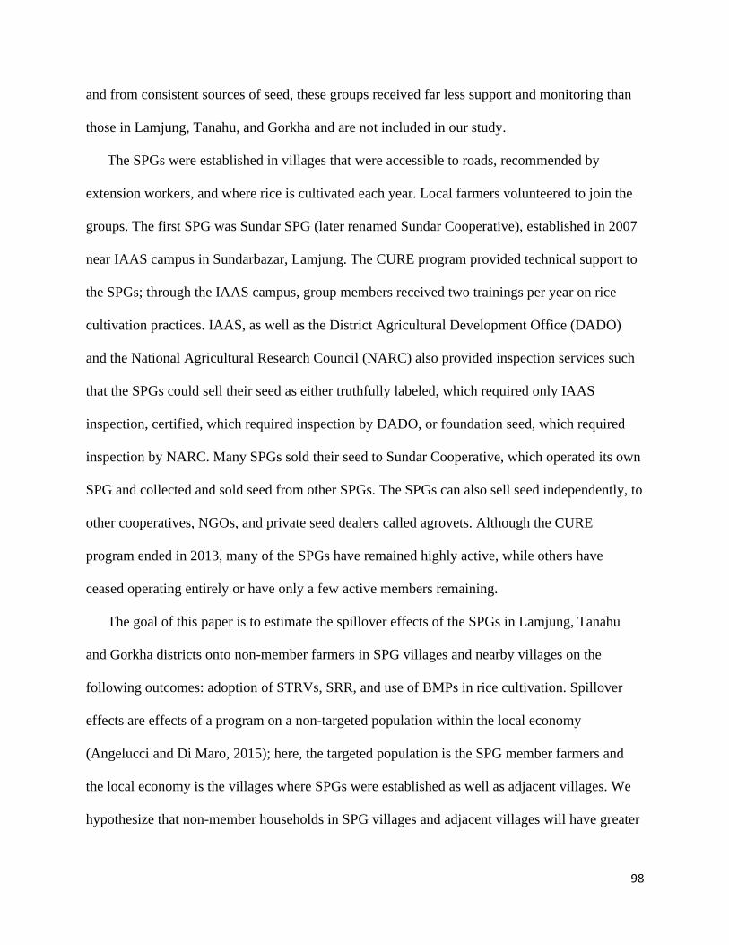
98
and from consistent sources of seed, these groups received far less support and monitoring than
those in Lamjung, Tanahu, and Gorkha and are not included in our study.
The SPGs were established in villages that were accessible to roads, recommended by
extension workers, and where rice is cultivated each year. Local farmers volunteered to join the
groups. The first SPG was Sundar SPG (later renamed Sundar Cooperative), established in 2007
near IAAS campus in Sundarbazar, Lamjung. The CURE program provided technical support to
the SPGs; through the IAAS campus, group members received two trainings per year on rice
cultivation practices. IAAS, as well as the District Agricultural Development Office (DADO)
and the National Agricultural Research Council (NARC) also provided inspection services such
that the SPGs could sell their seed as either truthfully labeled, which required only IAAS
inspection, certified, which required inspection by DADO, or foundation seed, which required
inspection by NARC. Many SPGs sold their seed to Sundar Cooperative, which operated its own
SPG and collected and sold seed from other SPGs. The SPGs can also sell seed independently, to
other cooperatives, NGOs, and private seed dealers called agrovets. Although the CURE
program ended in 2013, many of the SPGs have remained highly active, while others have
ceased operating entirely or have only a few active members remaining.
The goal of this paper is to estimate the spillover effects of the SPGs in Lamjung, Tanahu
and Gorkha districts onto non-member farmers in SPG villages and nearby villages on the
following outcomes: adoption of STRVs, SRR, and use of BMPs in rice cultivation. Spillover
effects are effects of a program on a non-targeted population within the local economy
(Angelucci and Di Maro, 2015); here, the targeted population is the SPG member farmers and
the local economy is the villages where SPGs were established as well as adjacent villages. We
hypothesize that non-member households in SPG villages and adjacent villages will have greater

99
adoption of STRVs and a higher SRR due to their improved access to STRV and other improved
rice seed varieties. We also hypothesize that non-member households in SPG villages will have
higher rates of BMP use, as their close proximity to SPG members may expose them to greater
knowledge of BMPs. This increase in BMP utilization may not extend to neighboring villages
however, as they are more likely to spread amongst farmers who either know one another or who
observe one another’s rice fields. We do not examine the impacts of the SPGs that were
established in Bajhang because these had little support from the CURE program.
We are interested in the spillover effects of SPGs because the technologies that they use
(BMPs) and produce (STRVs, other improved rice seed) are highly transferrable to other farmers
within their communities, which can enhance spillover effects (Winters et al., 2011). In fact,
when technologies are highly transferrable, spillover effects can exceed direct program impacts,
and ignoring these spillover effects can drastically underestimate the impact of a program
(Winters et al., 2011). In addition, while existing literature has documented the benefits of SPGs
and other organized forms of seed production such as contracts on producing farmers (Simmons
et al., 2005; Winters et al., 2010; Katungi et al., 2011; Mishra et al., 2016; Tebeka et al., 2017),
there is no research to our knowledge that examines spillover benefits of seed production, which
is surprising given that the main technology produced by SPGs, seed, is designed to be
sold/transferred to other households.
Previous studies found that SPGs and other forms of seed production are beneficial for
producers. Katungi et al. (2011) found that farmer-based bean seed production in Kenya was
profitable for producer farmers, despite the higher costs of producing bean seed over bean grain.
Tebeka et al. (2017) examined community-based seed multiplication of common bean in
Ethiopia and found that producing and selling seed is more profitable for farmers than producing

100
and selling grain. Contracts to produce hybrid maize seed and broiler chickens have proven
beneficial for smallholder farmers in Indonesia, improving returns to farm capital, although
contracts to produce rice seed did not increase returns (Simmons et al., 2005). In Nepal, Mishra
et al. (2016) found that farmers who entered into contracts with private seed companies for the
production of high yielding rice varieties earned higher profits than farmers who produced high
yielding varieties independently.
There is a significant literature arguing the importance of estimating spillover effects, due to
the fact that indirect effects of interventions, particularly agricultural and health interventions,
can arise for many reasons (Winters et al. 2011; Benjamin-Chung et al., 2015). For agricultural
programs, positive externalities exist if agricultural practices can be transferred from farmer to
farmer, and general equilibrium effects can occur if a project changes input or output prices
(Winters et al. 2011). Benjamin-Chung et al. (2015) outline many ways in which spillover effects
can arise from health interventions: learning/imitation effects (the untreated population may
learn new skills or behaviors from the treated), norm shaping (the treated population may change
social norms, which the untreated follow passively), and general equilibrium effects (changes in
prices or other aspects of the economy that change economic behaviors of community members).
Although these authors focus on health interventions, the same effects could arise from
agricultural interventions, including SPGs.
Empirical studies have found evidence of spillover effects of many different types of
development programs. Miguel and Kremer (2004) investigated a project in Kenya that provided
deworming medicine to some students in randomly selected schools and found high evidence of
spillover effects: untreated students in selected and neighboring schools also experienced
improved health and school participation due to treatment externalities that likely arose from a

101
reduced number of worms in the environment. Thome et al. (2013) found evidence of spillover
effects on the value of local agricultural production arising from general equilibrium impacts of a
cash transfer program in Kenya. Wanjala and Muradian (2013) found that spillover effects on
production margins and household income arose from the Millennium Village Project in Kenya.
Finally, Haile et al. (2017) estimated the impacts on households who participated in a
participatory action research program in Malawi. This program selected villages, and households
within those villages volunteered to participate, similar to how the CURE program selected
villages for SPGs in Nepal. The authors found evidence of positive program impacts, but noted
the difficulty of evaluating the effectiveness of the program due to possible spillover effects onto
other households within the program villages. Because we hypothesize that spillover effects of
the CURE SPGs could be very high for non-members within and near SPG villages, we estimate
these effects explicitly.
Haile et al. (2017) note another difficulty in estimating program impacts: the possibility that
unobserved village characteristics could bias effect estimates. This is a potential problem in our
study, as well, because villages were not chosen randomly for the establishment of SPGs. We
control for potential selection bias by using two different propensity-score weighted regression
adjustment estimation methods. These methods estimate both the treatment model (generating
propensity scores, or the probability that each village was treated), and the outcome model. By
weighting the outcome model using the propensity scores, these estimation methods improve the
balance between treated and untreated groups, and are considered to be “doubly-robust,” as they
are valid if either the treatment or outcome model is incorrectly specified (Wooldridge, 2010).
They also allow for multi-valued treatment effects, which we need as we are interested in
spillover effects onto two separate groups: non-members in SPG villages and non-members in

102
adjacent villages. These methods only reduce bias arising from observed village characteristics.
In the case of SPG village selection, some traits that were considered for selection are easily
observable: distance to roads and rice being grown each year. However, unobserved bias could
arise as if we cannot observe all factors that influenced extension workers’ village
recommendations. While we include several village-level covariates that could have influenced
these recommendations, we also perform statistical tests to examine whether unobserved bias, or
endogeneity, is likely to bias our results.
This research has implications for policy makers in Nepal and other Asian countries who
wish to increase the supply and adoption of improved agricultural technologies. It will provide
evidence as to whether the scaling up of similar IFAD-funded or other projects that focus on
community-based seed production is an effective way to protect communities from drought and
other climate stressors through the spread of agricultural technologies.
2. Data We conducted three types of surveys in Lamjung, Tanahu and Gorkha districts of Nepal
(shown in Figure 4-1) for the CURE impact evaluation. The first was an SPG leader survey, in
which we interviewed executive committee members of the 12 SPGs established by CURE in
Lamjung, Gorkha, and Tanahu districts in September-October, 2018. The second was a
household survey in which we interviewed randomly selected households in the three districts
regarding their 2018 monsoon season rice production, household demographics, credit usage and
asset ownership. Finally, we conducted a community survey in which we interviewed village
leaders in each selected village about village amenities, access to extension, sources of rice seed,
etc. The household and community surveys were administered between November 26, 2018 and

103
December 20, 2018. The monsoon season runs from July to November each year, so data
collection occurred shortly after the end of the season.
Figure 4- 1: Map of Nepal showing CURE districts
The SPG leader survey was a focus group survey in which we interviewed 3-6 executive
committee members from each SPG. It was conducted a month prior to the household and
community surveys so that it could inform the household survey regarding specific rice varieties
and best management practices about which to collect data. The SPG leader survey collected
basic information on year that the group was established, membership history, and services
available to members. A detailed module on training asked questions on when, where, and by
whom SPG members were/are trained. We also asked specific questions regarding how SPG
members were trained on planting methods, fertilizer application, weed and pest management,
and processing seed after harvest. Finally, we collected the complete list of varieties each SPG
has ever grown and which of these varieties are STRVs. The purpose of this was to put together
a list of BMPs and STRVs to ask about in the household survey. Information on the quantity of

104
seed produced in 2017 and sold in 2018, the most recent years of production and sales, and
quantities sold to different buyers in different locations (for instance, agrovets, extension
agencies, and local markets) was collected. We also collected information on rice storage:
whether the SPG has a storage facility, its capacity and the year it was built, and the location(s)
where the SPG members stored rice in 2018. Finally, the survey asked about current challenges
the SPGs face and what resources could help them overcome these challenges.
For the household survey, we interviewed 900 households in 75 villages (12 households per
village) across Lamjung, Tanahu and Gorkha districts. These 75 villages included the 12 villages
with SPGs. We also randomly selected one adjacent village to each of these (12 in total) in order
to capture spillover effects of the SPGs onto neighboring villages. The remaining 51 villages
were randomly selected to be representative of rice-growing households in the surrounding
Village Development Committees (VDCs)15. Our sampling frame included VDCs that contained
the SPG villages as well as each VDC that was adjacent to these or that connected them into one
continuous area, for a total of 41 VDCs (Figure 4-2). We chose this study area because it covers
a range where dissemination of SPG seeds is realistic, while still containing villages that vary by
distance to SPGs, access to roads, elevation, and other factors that could affect adoption of
STRVs.
We determined the number of villages to randomly sample from each district based upon
district total population, leading to 14 randomly selected villages in Gorkha, 22 in Lamjung, and
27 in Tanahu. Because lists of villages and households were not available, staff from a local
NGO called CHESS Nepal collected this information. To ease this process, we first randomly
selected wards in our study area using proportional to population size sampling (each VDC
15 VDCs are administrative units in Nepal that are smaller than districts but larger than villages.

105
contains wards numbered 1-9 and each ward contains about 3-6 villages). Once the names of
villages and their approximate number of rice-growing households from each of the selected
wards was collected, we randomly sampled one village per ward, again using proportional to
population size sampling. These randomly selected villages and the SPG/SPG-adjacent villages
are located in 37 of the 41 VDCs in our study area; thus, our sample covers a wide range of the
study area.
Once villages were selected, CHESS Nepal collected a list of all rice-growing households
within each sampled village. Twelve households were randomly selected from each village in
addition to five alternate households in case selected households were not available on the day of
survey enumeration. The study area VDCs as well as locations of SPGs and sampled households
are shown in Figure 4-2.
Figure 4- 2: Map of Lamjung, Tanahu and Gorkha districts showing study area:
Note: Some households appear to be outside of study area VDCs; this is likely due to fuzziness of border
boundaries on the ground
#
#
#
#
#
#
#
#
#
##
#
Study Area
Legend
# SPG Locations
Households
Study Area VDCs
Lamjung, Tanahu, and Gorkha Districts

106
To administer the household and community surveys, we hired twelve enumerators. Each
enumerator had or was pursuing an undergraduate degree related to agriculture. Most of the
enumerators had previous survey experience, and many had worked previously with our partner
organization, iDE Nepal. The remaining enumerators were selected for interviews based on the
recommendations of faculty at IAAS.
The household survey began with a household roster, followed by a module on STRV
adoption. Households were asked if they had ever heard of each of the improved drought-tolerant
varieties grown by SPGs. If the household reported having heard of the variety, we asked when
they first heard of it and from where/whom, if they had ever grown it, in which season they first
grew it, and where they obtained their initial planting material.
The bulk of the remaining survey collected detailed information on rice cultivation during the
2018 monsoon season, as well as some information on rice cultivation in the 2017 monsoon
season. The plot roster module collected basic information on all plots cultivated by the
household in the 2018 monsoon season such as size, land ownership, crops grown, and whether
the crops have suffered from insufficient water availability in the past five years. For plots under
rice cultivation that season, more detailed questions regarding irrigation, fertilizer and pesticide
use, and paid and unpaid labor were asked. Half of the households received an extended version
of this module, which included questions regarding the type of fertilizer applied, timing of
fertilizer application and weeding, and more detailed questions about labor activities. The next
module collected information on each rice variety grown by the household in the 2018 monsoon
season, including the source of planting material, the year the household first grew the variety,
and whether they identify it as an improved and/or drought-tolerant variety. To assist in varietal
identification, we asked a series of questions including when the household first grew the variety

107
and where they obtained the planting material, whether they thought it was improved or local,
and drought-tolerant. The survey then collected information at the variety-plot level for both
2018 and 2017, since more than one rice variety can be grown per plot; specifically, plot area
cultivated under each variety, quantity of seed planted, method of planting, and quantity
harvested.
Remaining household survey modules asked about social capital, access to agricultural
extension, and asset ownership. We collected GPS coordinates for all interviewed households,
which we combined with Landsat data (National Center for Atmospheric Research Staff, 2018)
to calculate the Normalized Difference Vegetation Index (NDVI), a measure of the extent of
green vegetation that ranges from -1 (a body of water) to 1 (rain forest), OpenStreetMap
(OpenStreetMap contributors, 2018) road data to calculate the distance from each household to
the nearest road, and elevation data to calculate the slope of land on which each household
resides.
The community survey, administered at the same time as the household survey, collected
information from village leaders on amenities and services availability within the villages. This
included distance to the nearest asphalt road, agrovet, and DADO, which provides extension
services. We also asked about adoption of STRVs at the village level and whether local names
were used for any of the STRVs varieties to further assist in correct varietal identification.
The success of our study relies on households accurately identifying the rice varieties they
cultivated, particularly the STRVs. Prior to conducting the household survey, we asked local
extension agents, agrovets, other individuals knowledgeable about rice production within the
study area about farmers’ ability to identify varieties. All reported that farmers are well aware of
the official names of the varieties they cultivate, particularly the more recently released improved

108
varieties including the STRVs. They stated that the only problem that could arise was that
farmers in different villages could have different names for local varieties. To help in proper
varietal identification during data collection, we put together a list of variety names from which
enumerators could select. This list came from the SPG leader survey and government documents
on rice varieties (Crop Development Directorate, 2015). For varieties named but not on our pre-
defined list, local experts helped classify whether they were improved, hybrid, or STRV. For the
purposes of this study, identification of STRVs is most crucial, and we feel very confident that
households were able to correctly identify these varieties.
3. Conceptual Framework A farmer is more likely to adopt a new agricultural technology (e.g. a new rice variety or
management practice) if he/she is aware of the technology and the benefits from doing so
outweigh the costs. Probability of awareness can depend on many factors, including access to
information within the community (from formal and informal sources) level of education, and
gender, as preferences and access to resources can vary by gender (Doss, 2001). The costs and
benefits of adoption also vary by community and household and can depend on the actual cost of
the technology, ease of accessing the technology, farmer’s land type and size, and the availability
of complementary resources such as knowledge or agricultural inputs (Feder et al, 1985; Foster
and Rosenzweig, 2010).
SPGs bring resources into their communities including improved rice seed of STRV and
other varieties, as well as knowledge of improved management practices members receive as part
of their training. SPGs can have spillover effects onto local farmers through the following
mechanisms (Benjamin-Chung et al., 2015; Winters et al., 2011):

109
1. Improved rice seed becoming easier (and thus, less costly) to obtain for farmers
near SPGs. Similarly, general equilibrium effects can lower the price of seed
within the local economy due to increased production;
2. Learning/imitation effects: local farmers learn about new varieties and BMPs
from SPG members, either by talking with them or by observing them;
3. Norm-setting effects: SPG farmers may establish new social norms within the
village surrounding cultivation practices;
We hypothesize that non-SPG member farmers in SPG villages and nearby villages will have
a higher rate of adoption of STRVs than other farmers in the area, due to their proximity to SPGs
which increase farmers’ access to (and lower the costs of obtaining) STRV seed. Similarly, they
will have an increased SRR due to their improved access to STRV and other seed.
Learning/imitation, norm-setting, and general equilibrium effects could also contribute to this.
We also hypothesize that non-member farmers who live in SPG villages will be more likely
to adopt BMPs than farmers in all other villages, due to their proximity to SPG members who
received CURE training. These impacts arise primarily through learning/imitation and norm-
setting effects. This effect could be greater for practices that are more “visible” (e.g. crop
rotations) than those that are less visible (e.g. rice cleaning and drying), are easy and/or cheap to
implement, and/or are very profitable. The increase in BMP usage may not spread to adjacent
villages, as learning and norms may not extend as easily across villages compared to rice seed.
4. Empirical Framework
4.1. Outcomes of Interest and Treatment Variable
Table 4-1 defines our outcomes of interest in evaluating the spillover effects of SPGs. We
examine adoption of STRVs in three time periods: any season up to and including the 2018
monsoon season; the 2017 monsoon season; and the 2018 monsoon season. This is to capture

110
trends over time, allowing us to examine whether impacts of SPGs have become stronger or
weaker over time. The SRR is calculated as the percentage of seed grown by the household in
2018 that came from certified or truthfully labeled seed. Our list of BMPs comes from interviews
with SPG executive committee members about topics on which they were trained, and span
practices from the beginning of the rice season (pre-transplanting) to the end (post-harvest
processing). More information on these practices is provided in Section V.a of this paper, which
describes the results from the SPG leader survey.
Table 4- 1: Dependent variables
Outcome variable Description
STRV adoption Household has grown an STRV in the current or any previous season
STRV adoption (2018) Household grew an STRV in monsoon season of 2018
STRV adoption (2017) Household grew an STRV in monsoon season of 2017
SRR Seed Replacement Rate of rice at the household level, measured by the
% of seed that was grown from certified or truthfully labeled seed in
the 2018 monsoon season
Use of BMPs: Household practiced the following in 2018:
o Clean rice seed prior
to planting
Rice seed was cleaned prior to planting; either by floating it in water
and removing seeds that float to the top and/or picking through it to
remove damaged seeds
o Seeding ratio Quantity of rice seed planted in kg/hectare of land cultivated under rice
o Age of seedlings Age of seedlings in days when they were transplanted into rice fields
o Organic fertilizer Quantity of organic fertilizer in kg applied per hectare of rice land
o Chemical fertilizer Quantity of chemical fertilizer in kg applied per hectare of rice land
o Roguing Number of times the household rogued their rice fields
o Moisture testing Moisture of seed was checked prior to storage, either using a moisture
control machine or by biting the seed to determine if it snaps in half
o Legume cultivation Household grew lentils
o Vegetable cultivation Household grew vegetables
We quantify the impact of living in an SPG village or an adjacent village on the outcome
variables defined in table 4-1 using multivalued treatment effects models. We specify the
treatment variable as the multi-valued categorical treatment variable 𝑆𝑃𝐺𝑚, where m refers to
individual villages. 𝑆𝑃𝐺𝑚 = 0 for control villages, i.e. those that were randomly selected. 𝑆𝑃𝐺𝑚
is equal to 1 if village m is adjacent to an SPG village and 2 if village m is an SPG village.

111
4.2. Doubly-Robust Weighted Regressions
The challenge of estimating the impact of 𝑆𝑃𝐺𝑚 on our outcomes of interest is that SPG
villages were not chosen randomly by CURE program staff. Therefore, we would expect that
SPG villages, and possibly adjacent villages, may vary systematically from randomly selected
villages. If some of this variance is correlated with our outcome variables, then our treatment
effect estimates will be biased.
To control for this bias, and to ensure that our treatment and control villages are comparable,
we use two weighted regression estimators: the augmented inverse-probability weighted (AIPW)
estimator and the inverse-probability weighted regression adjustment (IPWRA) estimator. We
also estimate unweighted regression adjustment (RA) estimators as is commonly done in the
weighted regression estimator literature (Smale et al. 2018; Haile et al. 2017).
Weighted estimators work similarly to RA estimators, but involve an extra step (the
weighting). RA estimates the outcome model using a linear, logit, probit, or Poisson model,
where the outcome variable 𝑌𝑖 is regressed on covariates 𝑋𝑚𝑖 which vary by village m and
household i, and 𝑍𝑚, which vary by village m.
𝑌𝑖 = 𝑓(𝑋𝑚𝑖, 𝑍𝑚, Β) + 𝜖𝑚𝑖 + 𝜖𝑚 (1)
The error terms 𝜖𝑚𝑖 and 𝜖𝑚 are the household and village level error terms, which are
assumed to be independent and, in our models, robust to heteroskedasticity. Then, RA involves
averaging the predicted outcomes for each treatment level (0-2) of 𝑆𝑃𝐺𝑚. The third step of the
RA consists of calculating the difference between the two treatment groups (1-2) and the control
group, which gives the average treatment effect for each level of treatment.
Weighted estimators add the weighting which involves the following steps. First, the
treatment model is estimated using a multinomial logit model for multi-valued treatments, where

112
the treatment is regressed on a set of village characteristics represented by the vector 𝑍𝑚 in
equation (2)
𝑆𝑃𝐺𝑚 = ℎ(𝑍𝑚, Λ) + 𝑤𝑚 (2)
The error term 𝑤𝑚 includes any village heterogeneity in treatment not captured by 𝑍𝑚, and Λ
is a vector of parameters to be estimated. Then, the generalized propensity score is calculated:
this is the conditional probability that a village receives each specific level of treatment (𝑆𝑃𝐺𝑚
= 0, 1, 2) given 𝑍𝑚. The outcome regression models (in IPWRA) for each treatment level or the
computed averages for each treatment level (in AIPW) are then weighted by the inverse of the
propensity score for the respective treatment level (McCaffrey et al., 2013). The variables in 𝑍𝑚
can overlap with the variables in 𝑋𝑚𝑖, but they do not have to. In our models, 𝑍𝑚 only includes
variables captured at the village level because treatment is at the village level.
Weighted estimators create a more balanced data set based on observable characteristics than
RA or other unweighted regression methods such as OLS or logit outcome models, making
treatment and control observations more comparable to each other and further reducing the bias
that arises from observables (Austin, 2011). Weighted estimators are called “doubly robust”
because they only require that either the outcome model or the treatment model be correctly
specified (Wooldridge, 2010). An additional advantage is that they allow for multi-valued
treatment effects, which our regressions require (Cattaneo, 2010; Smale et al. 2018). Both
IPWRA and AIPW have been used in recent literature evaluating the impacts of agricultural
interventions. Smale et al. (2018) use multivalued AIPW and IPWRA estimators to evaluate the
effects of hybrid sorghum adoption on household sorghum yields and purchases, and dietary
diversity. Esposti (2017) uses multivalued AIPW to estimate the impacts of the Common
Agricultural Policy on farm production choices of farmers in Italy. Haile et al. (2017) use the

113
AIPW estimator to determine the effects of participatory action research in Malawi. Finally,
Cavatassi et al. (2011) use inverse propensity score weighted least squares (a different type of
weighted estimator) to evaluate the impacts of Plataformas, a program in Ecuador that links
smallholder potato producers with agricultural support service providers.
Weighted regression estimators rely on two major assumptions: overlap and
unconfoundedness. The overlap assumption requires that the values of the weighting variables
𝑍𝑚 are similar enough between treatment and control villages that these villages can be
meaningfully compared. We assess the overlap assumption by examining the distribution of the
propensity scores for treatment and control groups. When a group has a high density of
propensity scores in the same range as the other groups, there is a high level of overlap (Imbens
and Wooldridge, 2007).
The unconfoundedness assumption stipulates that there are no unobserved village
characteristics that are both correlated with being selected for an SPG and our outcomes of
interest. We control for observed characteristics known to have influenced selection of SPG
villages, but if unobserved characteristics exist then selection bias could arise. A common way to
assess the validity of the unconfoundedness assumption is to verify that the weighting models
properly balance the covariates (Haile et al., 2017; Esposti, 2017). We do this using a balance
test derived by Imai and Ratkovic (2014).
Our set of weighting and control variables (𝑍𝑚) include village-level variables that likely had
an impact on selection of villages for SPGs (table 4-2). Proximity to roads was an explicit
criterion for SPG location; we therefore include distance from the village center to asphalt road
in minutes travel time using the most common mode of transportation. In addition, all SPG
villages were villages in which farmers grew rice every year. While all of our villages (SPG,

114
adjacent, and randomly selected) are villages where rice is grown each monsoon season, we
include a few agro-ecological variables to control and weight for suitability of rice production.
These include village averages for altitude, NDVI, and slope. We also include distance to IAAS
campus in minutes travel time, as CURE program implementers may have been more familiar
with, and thus more likely to select, nearby villages. Similarly, we include distance to the nearest
DADO, as extension agents may have been more likely to recommend villages near their offices.
Finally, we include distance to the nearest agrovet. Villages close to agrovets may be more likely
to experiment with different varieties, and thus be assessed as more likely to sustain a successful
SPG by CURE.
Our set of variables 𝑋𝑚𝑖 includes one village characteristic and several household
characteristics that could be correlated with both treatment and the outcome variables (table 4-2).
The village level variable used as a control is a dummy variable equal to one if the village had a
farmer’s association 6-10 years ago, around the time of the SPG establishment. We initially
wanted to include it as a weighting variable but it impaired overlap significantly. Moving it to
the control variable list 𝑋𝑚𝑖 did not change results substantially, thus we removed the presence
of a farmer’s association 6-10 years ago from the 𝑍𝑚vector. We believe it is an important to
control for this variable as farmer’s associations can improve access to information within a
village that could influence adoption of STRVs, SRR, and BMPs (Foster and Rosenzweig, 2010;
Beyene and Kassie, 2015).
We control for a number of household characteristics. The first is whether any household
member has ever been a member of an SPG. Controlling for membership is essential to separate
out the direct impact of belonging to a SPG from the spillover effects onto non-members. We
also control for the age, sex, and education of the head of household, as these traits could

115
influence access to information and other resources related to our outcomes of interest.
Households whose head is more educated may be more likely to replace rice seed according to
the recommended rate and adopt improved varieties and BMPs since they likely have greater
access to and ability to process information. Education enters the models as a binary variable
indicating whether the household head has completed primary education. The number of adults
in the household aged 15 and older is included as a measure of household labor availability as
labor availability could influence rice cultivation decisions including what varieties and practices
to use. We control for household wealth and resources using two variables: a wealth index
created using polychoric principal components analysis based on housing characteristics and
asset ownership in 2008, and a variable for land owned (in hectares) in 2008. Wealthier
households and households owning more land may be more likely to replace rice seed and to
adopt new varieties, as they have a greater ability to purchase seeds, and have access to more
resources that may promote adoption (Feder et al., 1985). We use information from 2008 to
avoid any potential endogeneity problem that could arise if SPGs have increased household
wealth or land ownership over time. Finally, distance to the nearest road can influence household
rice cultivation by affecting how easy it is for households to access new planting material as well
as information.

116
Table 4- 2: Village and household level covariates
Variable Description
Weighting variables (𝑍𝑚)
Altitude Average village altitude
NDVI Average village NDVI
Slope Average village slope
IAAS Average village distance to IAAS in minutes traveling by car
DADO Distance from the village center to the nearest DADO office in km
Agrovet Distance from the village center to the nearest agrovet in minutes
traveling using the most popular mode of transportation
Asphalt road Distance from the village center to the nearest asphalt road in
minutes traveling by the most popular mode of transportation
Control variables (𝑋𝑖𝑚)
SPG Member Has anyone in the household ever been a member of an SPG?
Sex Sex of the head of household
Age Age of the head of household
Education Did the head of household complete at least a primary education? (1
= yes)
Land owned, 2008 Quantity of land owned, in ha, in 2008
Wealth index quintile, 2008 Wealth index created using polychoric principal components
analysis based on asset ownership and housing characteristics in
2008
Distance to road Distance from household to the nearest road
Farmer’s association Did the village have a farmer’s association at least 6 years ago?
4.3. Robustness Checks
We perform several robustness checks to assess the sensitivity of our results to model and
treatment variable specification. As first robustness check, we estimate unweighted OLS, logit,
Poisson and fractional logit models, depending on the outcome variable, controlling for variables
in 𝑍𝑚 and 𝑋𝑖𝑚 and using as treatment variable distance to the nearest SPG measured in km and
then in minutes travel time. Having two measures for distance to the nearest SPG serves as a
sensitivity check of the results to the treatment variable specification. Moreover, using a
continuous variable sheds light on how far spillovers effects can occur. Spillovers could
potentially reach beyond adjacent villages, particularly for adoption of STRVs as the transfer of
seeds can occur along marketing channels which can extend past neighboring villages.
We also estimate the direct effects of SPG membership on members using RA; our treatment
variable is a dummy variable equal to one if a household member has ever been a member of an

117
SPG and zero otherwise. It is more difficult to deal with the problem of unobserved bias when
examining direct effects of membership because members volunteered to join SPGs and are very
likely to be the most capable or entrepreneurial farmers within their villages. However,
examining the effects of SPG membership can shed light on whether the magnitude of the
estimated indirect effects are plausible by serving as upper bounds for spillover effects. For
example, if SPG members did not follow recommended BMPs, then it is unlikely that SPGs
would have an impact on the adoption of BMPs among non-members based on our conceptual
framework of how spillover effects arose.
5. Descriptive Statistics In this section, we first present key findings from the SPG leader interviews. Then,
descriptive statistics from the community surveys disaggregated by SPG villages, adjacent
villages, and randomly selected villages are discussed. This section concludes with descriptive
statistics from the household survey broken down by SPG members from any village, non-
members in SPG villages, non-members in adjacent villages, and non-members in randomly
selected villages.
5.1. SPG Leader Survey Statistics
Our SPG survey results yield extensive descriptive information on the SPGs. Each SPG had
active membership (figure 4-3), even the groups that did not produce rice in the 2017/2018
season (figure 4-4). Membership numbers ranged from 7 to 75. In some groups, not all members
sold rice seed in 2018 (the number of members who sold rice ranged from 7 to 52). Most
members live within the same village as their SPG, though some SPGs have members that come
from neighboring villages.

118
Figure 4- 3: SPG membership, 2018
The SPGs varied in how active they were as of 2018 (figure 4-4). Nine of the groups still
actively produce and sell rice seed (one in Gorkha, two in Tanahu, and six in Lamjung). The
remaining three groups did not sell any rice seed in 2018 (two in Gorkha and one in Tanahu).
The active groups produced between 200 kg and 16 mt of rice seed in 2017 to be sold in 2018.
Seven out of the twelve groups had their own (or a shared) storage facility. The three inactive
groups did not have dedicated storage facilities.
Not all groups provided information from the year prior (2016 production/2017 sales), but
judging by the information we recieved, it appears that production in 2016/2017 was higher than
in 2017/2018. Production in many of the groups was significantly higher in 2016/2017 compared
to 2017/2018. Bhrikuti produced over 9,000 kg; Saghan Bali produced 21,500 kg; Sundar
produced 20,500 kg; Pragati produced 15,000 kg. Even two of the smaller groups from
2017/2018 produced more in 2016/2017: Jaya Buddha produced 1800 kg and Chardi/Ramgha

119
produced 20,000 kg. We do not know why 2016 production tended to be higher than 2017
production.
Figure 4- 4: SPG production and sales in 2017/2018
We asked each SPG to list all rice seed varieties its members had ever produced. The groups
had cultivated nine drought-tolerant varieties: Sukkha-1, Sukkha-2, Sukkha-3, Sukkha-4,
Sukkha-5, Sukkha-6, DRR 44, Hardinath, and Radha-4 and one submergence tolerant variety,
Swarna Sub-1. Members also grew Sabitri, Ramdan, and Loktantra, which are varieties suitable
for rainfed conditions but not considered drought-tolerant (Adhikari, 2017). Additional varieties
produced and sold by SPGs are Makwanpur, Sunaula Sagunda, CR Sub-1, Kirbhan Sub-1, Chait-
5, Radha-9, Bindeswore, and Mansuli, which are other improved varieties.
Groups most commonly sold to farmers directly from the SPG storage facilities, to the
district agricultural development offices (DADO) located in district capitals, and to Sundar
Cooperative in Sundarbajar, Lamjung. Only two groups sold to agrovets in 2018. We spoke to

120
two local agrovets who reported that they used to purchase SPG varieties but have recently
stopped because they can buy cheaper seed from producers in the plains, or terai, region of
Nepal, particularly from nearby Chitwan district.
SPG leaders also reported what they learned about rice cultivation from their IAAS trainings.
They were trained on many topics, including nursery bed preparation, seeding ratio, land
preparation, weeding, input use, seed cleaning and storage. Respondents also reported that, prior
to training, the members of their SPGs did not follow many of these practices. Information from
these surveys, as well as supporting information from Bishnu Bilas Adhikari of IAAS, who was
responsible for training the SPGs, allowed us to put together the list of BMP outcome variables
(table 1).
Training topics considered for our BMPs ranged from the beginning of the rice season to the
end. Prior to planting seed in nursery beds, SPG members were trained to clean their rice seed by
floating it in water and removing seeds that float to the top. When planning how much seed to
plant and subsequently transplant into their rice fields, SPG members were trained to plant 2-3
kg of seed per one ropani of land (40-60 kg/ha). Prior to training, SPG members reported
planting over twice as much, and sometimes three times as much. SPG members were also
trained to transplant seedlings when they are 18-22 days old, and prior to June 30. They were
trained on fertilizer use for both nurseries and fields, although they were not given precise
fertilizer recommendations, as fertilizer needs can vary by soil type and quality. Specifically,
they were trained that there are no limits on the quantity of organic fertilizer they could apply,
and that if chemical fertilizer was required, the rice plants needed phosphorous and potassium in
addition to nitrogen. This was contrary to common practice, which was to apply only urea as a
chemical fertilizer, which supplies only nitrogen. After harvest, farmers were trained to ensure

121
that seed is dried prior to storage; they could do this using a moisture testing machine if
available, or a “bite-test”: if the seed snaps when bitten, it is dry enough to be stored. Finally, in
addition to rice cultivation, SPGs were also trained in cropping patterns; specifically, they were
trained on the benefits of growing lentils and vegetables on rice fields after the rice was
harvested. The ability to do this was enhanced by cultivating short-duration rice varieties, which
includes STRVs.
Finally, SPG leaders were asked about their group’s challenges regarding rice cultivation and
sales. The most commonly listed cultivation problems were lack of labor and lack of machinery.
These are exacerbated by the high level of migration from rural areas to urban areas in Nepal and
to other countries. The biggest problem, however, related to finding consistent buyers for their
rice seed. Some groups used to sell to Sundar Cooperative, but said that Sundar could no longer
purchase their seed. Some noted communication difficulties with Sundar. It was not entirely
clear what the problem was between the groups and Sundar. Sundar noted that a lack of labor
made it challenging to manage their cooperative. This problem relates to what the agrovets had
mentioned to us; seed production is cheaper in the terai region of the country, and the SPGs face
competition from seed producers there. Two of the more remote, inactive groups (Jaisitar and
Shree Radha) also noted transportation difficulties for selling seed, but other groups did not
mention this as a challenge.
5.2. Community Survey Descriptive Statistics
Villages where SPGs were established differ from other villages in terms of agroecology and
access to other resources and seed sources (roads, IAAS, farmer’s associations more than 5 years
ago, agrovets), which is not surprising since these villages were not chosen randomly. SPG
villages are at lower elevation than randomly selected villages, and have somewhat flatter slopes
than randomly selected villages (table 4-3). They also have a slightly lower average NDVI value

122
than adjacent and randomly selected villages, denoting less vegetation. SPG villages and
adjacent villages are closer to asphalt roads on average than randomly selected villages. Finally,
SPG villages are closer to IAAS than randomly selected villages.
Table 4- 3: Community Survey Descriptive Results
Randomly
selected villages
(Group 0)
Adjacent
villages
(Group 1)
SPG villages
(Group 2)
Statistically significant
differences
Average household altitude
(masl) 629.05 (33.56) 577.56 (41.62) 523.62 (24.89) 5% difference 0 vs 2
Average household slope 10.27 (0.78) 10.42 (1.24) 7.81 (1.19) 1% difference 0 vs 2
Average village NDVI 0.34 (0.01) 0.34 (0.01) 0.32 (0.01)
1% difference 0 and 1
vs. 2
Distance from village to
asphalt road, minutes travel
time 55.39 (9.11) 25.83 (6.57) 20.00 (10.44)
5% difference 1 and 2 vs
0
Average household distance
to IAAS campus, minutes
travel time 56.74 (4.03) 41.21 (10.00) 35.69 (8.78) 5% difference 0 vs 2
Village had a farmer’s
association more than 5 years
ago (1 = yes) 0.29 (0.06) 0.33 (0.14) 0.75 (0.13)
1% difference 0 vs 2;
5% difference 1 vs. 2
Distance to agrovet, minutes
travel time 87.06 (14.25) 32.08 (8.47) 23.75 (0.11)
1% difference 0 vs 1 and
2
Distance to DADO, km 16.75 (3.96) 11.00 (3.11) 14.47 (1.87) n 51 12 12
5.3. Household Survey Descriptive Results
SPG villages have a higher percentage of SPG members than adjacent and randomly
selected villages (figure 4-5). The difference between adjacent and randomly selected villages is
not significant. This is not surprising, as SPGs reported that most of their members live within
their villages. We present the remaining household descriptive statistics broken into four
categories in order to examine differences by both membership and village: SPG members from
any village (9.7% of the sample), non-members in SPG villages (10.1%), non-members in
adjacent villages (14.7%), and non-members in randomly selected villages (65.56%).

123
Figure 4- 5: SPG membership by village type
Adoption of STRVs varies greatly by membership and village type (figures 4-6 to 4-8).
Overall adoption rates among SPG members (76%) and non-members in SPG villages (59%) do
not vary significantly but all other groups have differences that are significant at the 5% level or
lower; adoption of STRVs is 50% for non-members in adjacent villages and 40% for non-
members in randomly selected villages. Adoption in individual seasons (2017 and 2018) is lower
than adoption overall. In 2017, non-members in randomly selected villages, who had the lowest
level of adoption at 19%, vary significantly from non-members in adjacent villages (29%) and
SPG members (37%) at a 5% level or lower. Other differences are not statistically significant. In
2018, adoption of STRVs among non-members in randomly selected villages (28%) and non-
members in adjacent villages (33%) is significantly lower than for SPG members (48%), while
the adoption rate of non-members in SPG villages (36%) do not vary significantly from that of
other groups.

124
Figure 4- 6: STRV adoption by membership and village type
The SRR is highest for SPG members (79%), followed by non-members in SPG villages
(64%) while non-members in adjacent and randomly selected villages have the lowest SRR
(about 52% each) (figure 4-7). SPG members plant their seedlings when they are about 1.3 days
younger than any other group (this difference is significant at a 5% level against all groups).
Non-members in SPG and adjacent villages plant their seedlings when they are about 0.7 days
younger than non-members in randomly selected villages (significant at a 5% level). SPG
members have the lowest seeding rate (47.9 kg/ha), which differs from the seeding rate of all
other groups at a 5% level or lower. Non-members in SPG villages also have a lower seeding
rate (80.9 kg/ha) than households in adjacent villages, a difference that is significant at 5%. SPG

125
members rogue their rice fields more times (1.83 compared to 1.46-1.53) in a season than any
other group (significant at 1%).
Figure 4- 7: Best management practices and SRR
Households use 135.88 kg of chemical fertilizer and 8,163.51 kg of organic fertilizer per ha
of rice land on average. There are no significant differences between groups for chemical
fertilizer (figure 4-8). However, SPG members use more organic fertilizer than any other group,
although the difference between SPG members and non-members in SPG villages is significant
at just the 10% level (figure 4-8).

126
Figure 4- 8: Fertilizer use
About 60-65% of households in our sample cleaned their seeds prior to planting; there are
no significant differences between groups (figure 4-9). By contrast, 39% of SPG members test
their seed moisture prior to storage which is over twice as likely as any other group; there are no
significant differences between the other groups (figure 4-10). SPG members and non-members
in SPG villages are equally likely to plant legumes (51 – 60%), and more likely to plant legumes
than non-members in adjacent and randomly selected villages, who are equally likely to do so
(about 40% in each group). SPG members are more than twice as likely than any other group to
plant vegetables (figure 4-11); 22% compared to 10% or less for the other groups (this difference
is statistically significant for each group).
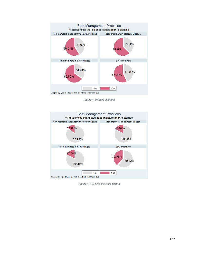
127
Figure 4- 9: Seed cleaning
Figure 4- 10: Seed moisture testing

128
Figure 4- 11: Legume and vegetable cultivation
Half of the respondents, selected at random, were asked more detailed questions about
fertilizer use and labor use on rice fields. We present descriptive statistics for these questions
disaggregated by membership status and village type, although we do not estimate econometric
models for these outcome variables. CURE training taught farmers that plants need more
nutrients than just nitrogen, and there is evidence that SPG members and non-members in SPG
villages are more likely to use additional inorganic fertilizers compared to non-members in other
villages; 83% of members and 89% of non-members in SPG villages used inorganic fertilizer
other than urea. This is significantly higher than for non-members in adjacent and randomly
selected villages, where 78% and 76% of respondents used non-urea chemical fertilizer,
respectively.
We examine labor requirements descriptively to explore whether the differences in
management practices lead to an overall increase or decrease in labor usage in rice cultivation for
SPG members. We find that labor usage varies somewhat by membership status and village type.
SPG members use less unpaid labor (138.5 person hours/ha) than non-members in randomly
selected (179.1) and adjacent villages (191.0), but a statistically equivalent quantity as non-

129
members in SPG villages. Non-members in SPG villages use the most paid labor (167.8 person
hours/ha); this varies significantly from non-members in adjacent villages (104.7); SPG members
and non-members in randomly selected villages fall in between. However, total labor usage
(unpaid plus paid) does not vary significantly by group. Therefore, changes in management
practices adopted by SPG members do not change total labor requirements; though they use less
unpaid labor than some other groups, their use of paid labor falls between that of the other
groups.
Table 4- 4: Household Characteristic Descriptive Statistics
Non-members in
randomly
selected villages
(Group 0)
Non-members in
adjacent villages
(Group 1)
Non-members
in SPG Villages
(Group 2)
SPG Members
(Group 3)
Statistically significant
differences
Sex of HoH (1 =
female)
0.21 (0.02) 0.17 (0.03) 0.27 (0.05) 0.29 (0.05) 10% difference 1 vs 2;
5% difference 1 vs 3
Age of HoH 51.99 (0.55) 52.80 (1.13) 51.03 (1.52) 52.21 (1.42)
HoH has primary
education (1 = yes)
0.68 (0.02) 0.71 (0.04) 0.82 (0.04) 0.77 (0.05) 1% difference 0 vs 2;
10% difference 0 vs 3;
10% difference 1 vs 2
Number of adults
in household
2.90 (0.05) 3.11 (0.12) 2.82 (0.15) 2.93 (0.14)
n 576 129 90 87 882
Land owned in
2008, m2
5560.81 (313.81) 5468.69 (455.61) 5268.08
(371.02)
6156.19
(640.33)
Wealth index in
2008
2.87 (0.06) 2.87 (0.12) 3.57 (0.15) 3.46 (0.14) 1% difference 0 vs 2 and
3; 1% difference 1 vs 2
and 3
n 587 128 90 87 892
Distance to road,
meters
46.82 (2.86) 47.53 (5.35) 27.52 (3.05) 40.83 (4.82) 1% difference 0 vs 2, 1%
difference 1 vs 2; 5%
difference 2 vs 3
n 590 132 91 87 900
Note: Differences in n across characteristics are due to missing observations.
Households in SPG villages tend to be better educated and were wealthier in 2008 than
households in other villages (table 4-4). They also lived closer to roads than non-members in
adjacent and randomly selected villages, though non-members in SPG villages live closer to
roads than SPG members. This result does not change if we look at only SPG members within

130
SPG villages, who live an average of 39.0 meters from roads. Non-members in adjacent villages
have a lower percentage of female-headed households than SPG member households. Non-
members in randomly selected villages have the lowest level of education, while non-members in
SPG villages have the highest. The differences that exist between these groups highlight the
importance of controlling for these factors and weighting our results to improve comparability of
villages.
6. Econometrics Results
6.1. Statistical Test Results
Propensity score overlap graphs are presented in the Appendix. For each treatment level (0-
2), a high proportion of villages from each group are in the area of common support (i.e. the area
where all groups have an above zero density of propensity scores), indicating that the overlap
assumption is met and our villages are comparable (Imbens and Wooldridge, 2007).
The Imai and Ratkovik test used to check balance between groups can only be estimated with
binary treatment variables. Therefore, to check balance, we specify treatment in three different
ways: SPG villages vs. randomly selected villages (we dropped adjacent village observations);
adjacent villages vs randomly selected villages (we dropped SPG village observations); SPG and
adjacent villages vs. randomly selected villages. For each specification, we fail to reject the null
hypothesis that our treatment model balances covariates between treatment groups (p = 0.178, p
= 0.390, and p = 0.999, respectively). This provides evidence that covariates are well balanced
and that the unconfoundedness assumption holds (Haile et al., 2017; Esposti, 2017).
6.2. STRV Adoption
Living in a village with an SPG raises the probability that a non-member household has
adopted an STRV at some point in the past by 17-18% above non-member households in
randomly selected villages (table 5), indicating the presence of spillover effects within villages

131
where SPGs were established. But there is no evidence that SPGs have spillover effects on
overall STRV adoption in adjacent villages. In 2018, non-members in SPG villages were about
15% more likely to have adopted STRVs than non-members in randomly selected villages
(though the IPWRA results were not significant). Compared to 2018, the effect of SPGs in 2017
on adoption of STRVs among non-members in SPG villages was stronger and spilled over onto
adjacent villages; SPGs raised adoption levels by 23-24% and 19-22% for non-members in SPG
villages and adjacent villages, respectively compared to non-members in randomly selected
villages. It is not surprising that spillover effects were greater in 2017 compared to 2018, as rice
seed production of SPGs was higher in 2017 than 2018. Our conceptual framework predicts that
the spillover effects of increased adoption will extend along market channels as far as SPG seed
is commonly sold, likely to adjacent villages. Given our results, there is evidence that spillover
effects may extend farther in years of high production.
Table 4- 5: Results for ra, ipwra, aipw models on impacts of SPGs on adoption of STRVs
Adoption in any season Adoption in 2018 Adoption in 2017
RA
ATE
IPWRA
ATE
AIPW
ATE
RA
ATE
IPWRA
ATE
AIPW
ATE
RA
ATE
IPWRA
ATE
AIPW
ATE
SPG
Village
0.17
(0.04)
***
0.18
(0.04)
***
0.18
(0.04)
***
0.15
(0.06)
***
0.13
(0.09)
0.15
(0.06)
***
0.23
(0.06)
***
0.24
(0.06)
***
0.23
(0.06)
***
Adjacent
village
0.02
(0.07)
0.06
(0.11)
0.02
(0.07)
0.11
(0.07)
0.17
(0.10) *
0.12
(0.07)
0.19
(0.10)
*
0.22
(0.07)
***
0.19
(0.10)
**
N 872 872 872 872 872 872 872 872 872
Note: */**/*** denotes statistical significance at 10%/5%/1% respectively. All standard errors are robust to
heteroskedasticity. Results provide comparison with SPG villages/adjacent villages to randomly selected villages.

132
6.3. Seed Replacement Rate
Results from the SRR estimation (table 4-6) indicate that the seed replacement rate is 52-53
percentage points higher for non-members in SPG villages compared to non-members in
randomly selected villages. Given our conceptual framework, we expected spillover effects onto
adjacent villages as well, but there is no evidence that this occurred. However, these results are
in line with the previous findings that SPGs did not stimulate STRV adoption in adjacent villages
in 2018; it would be interesting to determine if SPGs had an effect on SRR in 2017 but we only
have this data for 2018.
Table 4- 6: Results for ra, ipwra, aipw models on impacts of SPGs on SRR
SRR
RA ATE IPWRA ATE AIPW ATE
SPG Village 0.52 (0.20) *** 0.52 (0.21) ** 0.53 (0.20) ***
Adjacent village -0.03 (0.14) -0.10 (0.13) -0.03 (0.14)
N 869 869 869
Note: */**/*** denotes statistical significance at 10%/5%/1% respectively. All standard errors are robust to
heteroskedasticity. Results provide comparison with SPG villages/adjacent villages to randomly selected villages.
6.4. Best Management Practices
Non-members in SPG villages plant 56-59 fewer kg of seed per ha and rogue their rice seeds
almost one complete additional time compared to non-members in randomly selected villages.
Given the nature of the roguing outcome variable, which ranges from 0 to 5 times, estimating a
Poisson model would be most appropriate. However, given that these models would not
converge, a linear model was used to explain the number of time seeds were rogued. If we
remove the variable distance to agrovet, the Poisson models converge and results indicate that
non-members in SPG villages rogue their rice fields 0.59-0.64 times more than non-members in
randomly selected villages, though this difference is significant at the 10% level only. SPGs
increase the likelihood that non-members in adjacent villages will test the moisture of their seeds
by 13% compared to non-members in randomly selected villages. This effect on non-members in

133
SPG villages is not statistically significant but of greater magnitude than that in adjacent villages.
Finally, SPGs increase the likelihood that non-member households in SPG villages will grow
lentils during the monsoon season by 16-17% compared to non-members in randomly selected
villages.
Table 4- 7: Results for ra, ipwra, aipw models on impacts of SPGs on seeding ratio, roguing, moisture testing and legume
cultivation
Seeding Ratio Number of times
household rogued rice
fields
Tested moisture of seed
prior to storage
Grew legumes during
monsoon season 2018
RA
ATE
IPWRA
ATE
AIPW
ATE
RA
ATE
IPWRA
ATE
AIPW
ATE
RA
ATE
IPWRA
ATE
AIPW
ATE
RA
ATE
IPWRA
ATE
AIPW
ATE
SPG
Vill.
-59.60
(28.90)
**
-56.40
(26.35)
**
-59.37
(23.83)
**
1.16
(0.35)
***
1.26
(0.40)
***
1.16
(0.35)
***
0.25
(0.15)
*
0.23
(0.14)
0.24
(0.15)
0.17
(0.04)
***
0.16
(0.04)
***
0.16
(0.04)
***
Adj.
Vill.
23.84
(24.49)
25.26
(26.35)
23.83
(24.55)
0.03
(0.23)
-0.04
(0.23)
0.04
(0.23)
0.13
(0.03)
***
0.13
(0.04)
***
0.13
(0.03)
***
-0.10
(0.10)
-0.13
(0.08) *
-0.11
(0.10)
N 868 868 868 872 872 872 871 871 871 872 872 872
Note: */**/*** denotes statistical significance at 10%/5%/1% respectively. All standard errors are robust to
heteroskedasticity. Results provide comparison with SPG villages/adjacent villages to randomly selected villages.
Table 4- 8: Results for ra, ipwra, aipw models on impacts of SPGs on probability of cleaning seeds, quantity of chemical
fertilizer applied to rice fields, and age of seedlings at time of transplantation
Clean seeds Chemical Fertilizer Age of Seedlings
RA
ATE
IPWRA
ATE
AIPW
ATE
RA ATE IPWRA
ATE
AIPW
ATE
RA
ATE
IPWRA
ATE
AIPW
ATE
SPG
Village
0.01
(0.04)
0.01
(0.12)
0.00
(0.04)
95.75
(66.05)
135.87
(75.96)
-303.89
(252.72)
-1.63
(1.55)
-1.16
(1.53)
-1.67
(1.55)
Adj.
Village
-0.05
(0.07)
-0.02
(0.12)
-0.04
(0.07)
-308.66
(256.38)
-202.31
(172.0)
95.26
(66.32)
0.26
(0.75)
0.55
(0.75) *
-0.24
(0.75)
N 868 868 868 866 866 866 854 854 854
Note: */**/*** denotes statistical significance at 10%/5%/1% respectively. All standard errors are robust to
heteroskedasticity. Results provide comparison with SPG villages/adjacent villages to randomly selected villages.
For the Age of Seedlings regression, one randomly selected village had to be dropped because its propensity score
was too low for estimation.

134
There is no evidence of significant SPG spillover effects on non-member households in SPG
villages and adjacent villages for the probability that a household cleans seeds prior to planting,
the age of seedlings at time of transplantation, and the quantity of chemical fertilizer applied to
rice fields. Finally, the models examining whether SPGs impact the quantity of organic fertilizer
applied to rice fields and the probability that a household grows vegetables did not converge.
6.5. Robustness Checks
6.5.1. Distance to SPGs
To assess the sensitivity of the results to the treatment variable specification and explore how
far SPG spillover effects might travel, we estimated unweighted regressions with distance to the
nearest SPG as the treatment variable (controlling for the same variables). For continuous
outcome variables, we used OLS, for binary outcome variables, we used logit (marginal effects
are presented), and for outcome variables measured as a percentage, we used fractional logit
models. Living one km (one minute in travel time) farther from an SPG reduces the probability
that a non-member has adopted an STRV by about 2% (0.1-0.2%) at any point in time, in 2018
and in 2017. All effects are significant at the 5% level or lower except for the effect of one-
minute travel time in 2018 (table 4-9). This provides additional evidence that living in or nearby
an SPG village increases the likelihood of STRV adoption among non-members and indicates
that results are robust to treatment variable specification. These results also indicate that we may
have underestimated the spillover effects of SPG on STRV adoption if access to these seeds have
improved beyond adjacent villages. However, the spillover effect of SPGs on SRR in 2018 is not
significant when using distance to the nearest SPG as treatment variable. This is consistent with
the weighted results that suggest that SPGs spillover effects on SRR do not extend beyond SPG
villages, at least in 2018.
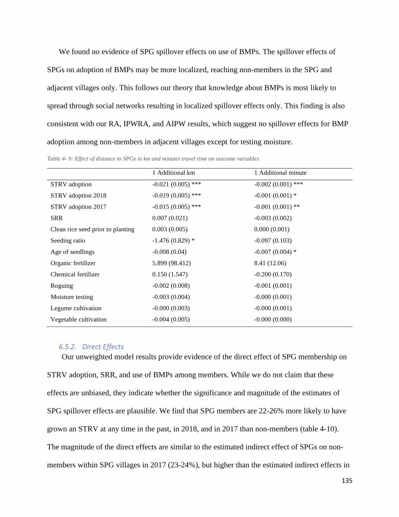
135
We found no evidence of SPG spillover effects on use of BMPs. The spillover effects of
SPGs on adoption of BMPs may be more localized, reaching non-members in the SPG and
adjacent villages only. This follows our theory that knowledge about BMPs is most likely to
spread through social networks resulting in localized spillover effects only. This finding is also
consistent with our RA, IPWRA, and AIPW results, which suggest no spillover effects for BMP
adoption among non-members in adjacent villages except for testing moisture.
Table 4- 9: Effect of distance to SPGs in km and minutes travel time on outcome variables
1 Additional km 1 Additional minute
STRV adoption -0.021 (0.005) *** -0.002 (0.001) ***
STRV adoption 2018 -0.019 (0.005) *** -0.001 (0.001) *
STRV adoption 2017 -0.015 (0.005) *** -0.001 (0.001) **
SRR 0.007 (0.021) -0.003 (0.002)
Clean rice seed prior to planting 0.003 (0.005) 0.000 (0.001)
Seeding ratio -1.476 (0.829) * -0.097 (0.103)
Age of seedlings -0.008 (0.04) -0.007 (0.004) *
Organic fertilizer 5.899 (98.412) 8.41 (12.06)
Chemical fertilizer 0.150 (1.547) -0.200 (0.170)
Roguing -0.002 (0.008) -0.001 (0.001)
Moisture testing -0.003 (0.004) -0.000 (0.001)
Legume cultivation -0.000 (0.003) -0.000 (0.001)
Vegetable cultivation -0.004 (0.005) -0.000 (0.000)
6.5.2. Direct Effects
Our unweighted model results provide evidence of the direct effect of SPG membership on
STRV adoption, SRR, and use of BMPs among members. While we do not claim that these
effects are unbiased, they indicate whether the significance and magnitude of the estimates of
SPG spillover effects are plausible. We find that SPG members are 22-26% more likely to have
grown an STRV at any time in the past, in 2018, and in 2017 than non-members (table 4-10).
The magnitude of the direct effects are similar to the estimated indirect effect of SPGs on non-
members within SPG villages in 2017 (23-24%), but higher than the estimated indirect effects in
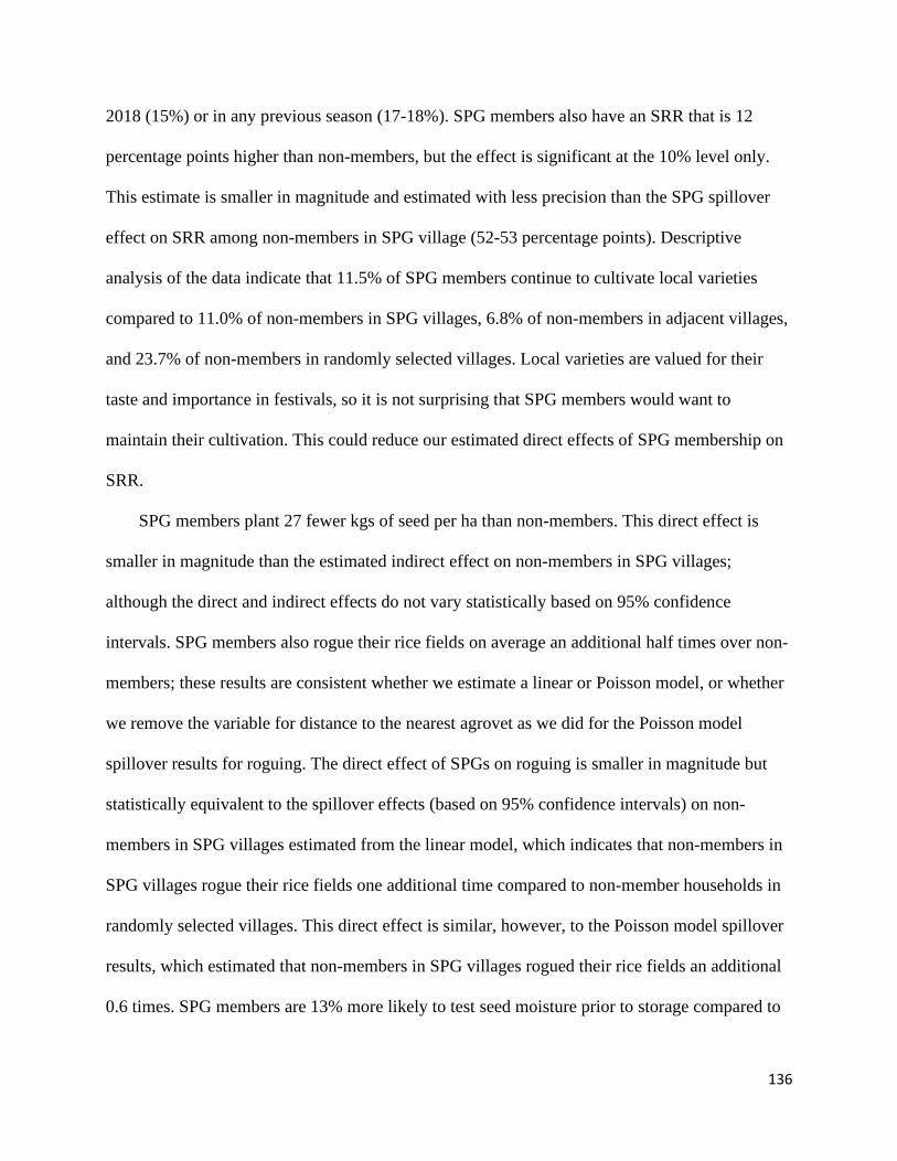
136
2018 (15%) or in any previous season (17-18%). SPG members also have an SRR that is 12
percentage points higher than non-members, but the effect is significant at the 10% level only.
This estimate is smaller in magnitude and estimated with less precision than the SPG spillover
effect on SRR among non-members in SPG village (52-53 percentage points). Descriptive
analysis of the data indicate that 11.5% of SPG members continue to cultivate local varieties
compared to 11.0% of non-members in SPG villages, 6.8% of non-members in adjacent villages,
and 23.7% of non-members in randomly selected villages. Local varieties are valued for their
taste and importance in festivals, so it is not surprising that SPG members would want to
maintain their cultivation. This could reduce our estimated direct effects of SPG membership on
SRR.
SPG members plant 27 fewer kgs of seed per ha than non-members. This direct effect is
smaller in magnitude than the estimated indirect effect on non-members in SPG villages;
although the direct and indirect effects do not vary statistically based on 95% confidence
intervals. SPG members also rogue their rice fields on average an additional half times over non-
members; these results are consistent whether we estimate a linear or Poisson model, or whether
we remove the variable for distance to the nearest agrovet as we did for the Poisson model
spillover results for roguing. The direct effect of SPGs on roguing is smaller in magnitude but
statistically equivalent to the spillover effects (based on 95% confidence intervals) on non-
members in SPG villages estimated from the linear model, which indicates that non-members in
SPG villages rogue their rice fields one additional time compared to non-member households in
randomly selected villages. This direct effect is similar, however, to the Poisson model spillover
results, which estimated that non-members in SPG villages rogued their rice fields an additional
0.6 times. SPG members are 13% more likely to test seed moisture prior to storage compared to

137
non-members, which is similar in magnitude to the spillover effect on non-members in adjacent
villages. SPG members are 19% more likely to grow lentils and 25% more likely to grow
vegetables than non-members. This direct effect for growing lentils is similar to the indirect one
for non-members in SPG villages. SPG members also transplant seedlings when they are on
average one day younger than non-members and use over 6,000 kg/ha more organic fertilizer on
rice plots than non-members. However, the effect of SPG membership on chemical fertilizer is
not significant. For age of seedlings, organic and chemical fertilizer use, we found no evidence
of spillover effects. Increasing organic fertilizer use could be costly for farmers, and this is why
this practice has not spilled over. In the case of seedling age, it could be that SPG members
transplant seedlings one day earlier than non-members but there is a lack of spillover effects
because this practice is not easily visible to other farmers.

138
Table 4- 10: RA direct effects of SPGs on SPG members for all outcome variables
SPG Membership
STRV adoption 0.22 (0.08) **
STRV adoption 2018 0.26 (0.08) ***
STRV adoption 2018 0.23 (0.06) ***
SRR 0.12 (0.06) *
Clean rice seed prior to planting -0.08 (0.06)
Seeding ratio -26.87 (7.13) ***
Age of seedlings -1.00 (0.50) **
Organic fertilizer 6667.05 (2673.16) **
Chemical fertilizer -37.42 (49.60)
Roguing 0.41 (0.11) ***
Moisture testing 0.13 (0.06) **
Legume cultivation 0.19 (0.05) ***
Vegetable cultivation 0.25 (0.07) ***
7. Conclusions Although the CURE program officially ended in Nepal in 2013, most SPGs in Lamjung,
Tanahu and Gorkha districts (9/12) are still actively producing and selling rice seeds, and
members still follow many of the BMPs they learned from their CURE training. SPGs that
struggled had trouble finding buyers for their seed. Seed produced in the Terai region is sold in
the districts at a lower price; as a result, agrodealers are less willing to purchase SPG seed.
Sundar Cooperative, a major buyer of SPG seed, no longer buys from some of the SPGs. The
reasons for this are not entirely clear, but may be due to a lack of labor.
Our qualitative analysis of the SPG interviews suggests that helping groups establish and
maintain buyers may be crucial for group success. Sundar Cooperative was initially established
to both produce seed and serve as a buyer of the other CURE SPGs, but it no longer purchases
from some of the groups. Follow-up discussions with Sundar Cooperative could inform on the
types of initial and ongoing support that would be most helpful for them to continue purchasing

139
seed from other SPGs. It is clear from our qualitative interviews with SPG executives that it is
important to ensure that seed buying networks are well-established by the end of program to
increase the likelihood that SPGs will remain active once the program ends.
Our analysis provides evidence that the SPGs had several spillover effects, benefiting local
and adjacent communities. This includes greater adoption of STRVs and increased SRR among
non-members in SPG villages, and increased STRV adoption for non-members in adjacent
villages in 2017 compared to non-members in randomly selected villages We also find that SPGs
induced greater use of some, but not all BMPs, including reduced seeding ratios, increased
roguing, and increased legume cultivation among non-members in SPG villages compared to
non-members in randomly selected villages. Non-members in adjacent villages were also more
likely to test seed moisture prior to storage than non-members in randomly selected villages. We
hypothesize that legume cultivation and roguing may have spread due to the fact that they are
highly visible practices while seeding ratios and seed moisture checking may have spread
because they are easy to implement and have no-cost. However, more research is needed to
understand how/why some BMPs have spread and catch on locally, while others have not.
Our study provides evidence that a short-term program to establish and support SPGs can
have long-lasting impacts on members; in this case study, SPG members have continued to
produce and sell seed and use BMPs. Technology transfer also occurred, generating spillover
benefits onto non-member households in SPG and adjacent villages. This indicates that if we had
considered only direct effects of the CURE project, we would have significantly underestimated
its benefits (Winters et al., 2011). SPGs can help improve communities’ resilience to climate
change if climate-smart technologies are targeted. Members of future established groups could
be explicitly encouraged to share their knowledge of BMPs in order to enhance project benefits.

140
Chapter 4 Appendix
Figure A4- 1: Propensity score overlap graph: SPG village
Figure A4- 2: Propensity score overlap graph: SPG-adjacent village
Figure A4- 3: Propensity score overlap graph: Randomly selected village

141
Chapter 4 References Angelucci, M., Di Maro, V., 2015. Program Evaluation and Spillover Effects. Policy Research
Working Paper. World Bank, Washington, D.C.
Austin, P.C., 2011. An Introduction to Propensity Score Methods for Reducing the Effects of
Confounding in Observational Studies. Multivariate Behavioral Research 46, 399-424.
Benjamin-Chung, J., Abedin, J., Berger, D., Clark, A., Falcao, L., Jimenez, V., Konagaya, E.,
Tran, D., Arnold, B., Hubbard, A., Luby, S., Miguel, E., Colford, J., 2015. The identification and
measurement of health-related spillovers in impact evaluations A systematic review.
International Initiative for Impact Evaluation (3ie), London.
Beyene, A.D., Kassie, M., 2015. Speed of adoption of improved maize varieties in Tanzania: An
application of duration analysis. Technological Forecasting & Social Change 96, 298-307.
Cattaneo, M., 2010. Efficient semiparametric estimation of multi-valued treatment effects under
ignorability. Journal of econometrics 155, 138-154.
Cavatassi, R., Salazar, L., Gonzalez-Flores, M., Winters, P., 2011. How do Agricultural
Programmes Alter Crop Production? Evidence from Ecuador. Journal of Agricultural Economics
62, 403-428.
Crop Development Directorate, 2015. Rice Varietal Mapping in Nepal: Implication for
Development and Adoption. Department of Agriculture Hariharbhawan, Lalitpur.
Doss, C., 2001. Designing agricultural technology for African Women Farmers: Lessons from 25
Years of experience. World Development 29, 2075-2092.

142
Esposti, R., 2017. The heterogeneous farm-level impact of the 2005 CAP-first pillar reform: A
multivalued treatment effect estimation. Agricultural Economics 155, 373-386.
Feder, G., Just, R.E., Zilberman, D., 1985. Adoption of agricultural innovations in developing
countries: A survey. Economic development and cultural change 33, 255-298.
Foster, A.D., Rosenzweig, M.R., 2010. Microeconomics of technology adoption. Annual Review
of Economics 2, 395-424.
Gauchan, D., Thapa Magar, D.B., Gautam, S., Singh, S., Shankar Sing, U., 2014. Strengthening
Seed System for Rice Seed Production and Supply in Nepal. Nepal Agricultural Research
Council Socioeconomics and Agricultural Research Policy Division, Khumultar, Lalitpur.
Gonzales, P.G., Huelma, C.C., 2013. Module 5 Seed Health Improvement for Crop and Pest
Management. In: Manzanilla, D.O., Janiya, J.D., Johnson, D.E. (Eds.), Establishing community-
based seed systems: A training manual. IRRI, Los Banos (Philippines).
Haile, B., Azzarri, C., Roberts, C., Spielman, D.J., 2017. Targeting, bias, and expected impact of
complex innovations on developing-country agriculture: evidence from Malawi. Agricultural
Economics 48, 317-326.
Imai, K., Ratkovic, M., 2014. Covariate balancing propensity score. Journal of the Royal
Statistical Society Series B 76, 243-263.
Imbens, G., Wooldridge, J.M., 2007. Estimation of Average Treatment Effects Under
Unconfoundedness. What's new in Econometrics. NBER.
IRRI Rice Knowledge Bank, 2012. Quality Rice Seed. IRRI, Los Banos, Philippines.

143
Katungi, E., Karanja, D., Wozemba, D., Mutuoki, T., Rubyogo, J.C., 2011. A cost-benefit
analysis of farmer based seed production for common bean in Kenya. African Crop Science
Journal 19, 409-415.
Manzanilla, D.O., Johnson, D.E., Castillo, G.T., 2017. Overview. In: Manzanilla, D.O., Singh,
R.K., Kato, Y., Johnson, D.E. (Eds.), Climate-ready technologies: Combating poverty by raising
productivity in rainfed rice environments in Asia. International Rice Research Institute, Los
Banos, Philippines.
McCaffrey, D.F., Griffin, B.A., Almirall, D., Slaughter, M.E., Ramchand, R., Burgette, L.F.,
2013. A Tutorial on Propensity Score Estiamtion for Multiple Treatments Using Generalized
Boosted Models. Statistics in Medicine 32, 3388-3414.
Miguel, E., Kremer, M., 2004. Worms: Identifying Impacts on Education and Health in the
Presence of Treatment Externalities. Econometrics 72, 159-217.
Mishra, A.K., Kumar, A., Joshi, P.K., D'souza, A., 2016. Impact of contracts in high yielding
varieties seed production on profits and yield: The case of Nepal. Food Policy 62, 110-121.
National Center for Atmospheric Research Staff (Eds), 2018. The Climate Data Guide: NDVI:
Normalized-difference-vegetation-index: NOAA AVHRR.
OpenStreetMap contributors, 2018. Humanitarian Data Exchange OpenStreetMap Team Roads
(OpenStreetMap Export). licensed under the Open Data Commons Open Database License
(ODbL) by the OpenStreetMap Foundation (OSMF).
Simmons, P., Winters, P., Patrick, I., 2005. An analysis of contract farming in East Java, Bali,
and Lombok, Indonesia. Agricultural Economics 33, 513-525.

144
Smale, M., Assima, A., Kergna, A., Thériault, V., Weltzien, E., 2018. Farm family effects of
adopting improved and hybrid sorghum seed in the Sudan Savanna of West Africa. Food Policy
74, 162-171.
Tebeka, Y.A., Katungi, E., Rubyogo, J.C., Sserunkuuma, D., Kidane, T., 2017. Economic
performance of community based bean seed production and marketing in the central rift valley of
Ethiopia. African Crop Science Journal 25, 189-205.
Thome, K., Filipski, M., Kagin, J., Taylor, J.E., Davis, B., 2013. Agricultural Spillover Effects of
Cash Transfers: What does LEWIE have to say? American Journal of Agricultural Economics
95, 1338-1344.
Wanjala, B.M., Muradian, R., 2013. Can Big Push Interventions Take Small-Scale Farmers out
of Poverty? Insights from the Sauri Millennium Village in Kenya. World Development 45, 147-
160.
Winters, P., Maffioli, A., Salazar, L., 2011. Introduction to the Special Feature: Evaluating the
Impact of Agricultural Projects in Developing Countries. Journal of Agricultural Economics 62,
393-402.
Winters, P., Simmons, P., Patrick, I., 2010. Evaluation of a Hybrid Seed Contract between
Smallholders and a Multinational Company in East Java, Indonesia. The Journal of Development
Studies 41, 62-89.
Wooldridge, J.M., 2010. Econometric Analysis of Cross Section and Panel Data. The MIT Press,
Cambridge, MA and London, England.

145
Chapter 5: Conclusion Agricultural technologies can help address many of the world’s rural development
challenges. The goal of this dissertation is to examine how policy makers can implement
effective strategies to encourage adoption of these technologies, and how the technologies
themselves impact the well-being of rural households. It evaluates the effectiveness of different
distributional strategies for iron-biofortified beans, which are designed to improve nutrition, as
well as STRVs and BMPs in rice production, which aim to reduce vulnerability to climate
change. It also evaluates how adoption of an iron-biofortified bean variety can improve
household nutrition and food security through its impacts on bean yields, bean consumption, and
bean sales. Overall, it finds evidence that strategies to distribute agricultural technologies
influence adoption decisions of producer households, and that adoption can improve a number of
household outcomes.
The first paper provides evidence of the effectiveness of different delivery approaches at
speeding up adoption and reducing disadoption speed of iron-biofortified bean varieties in
Rwanda. This is important, as fast and sustained consumption of high iron beans is necessary to
achieve health improvements of iron-deficient household members. This paper contributes to the
literature on technology adoption by using duration models to analyze adoption, disadoption, and
readoption speed, allowing us to model adoption as a complex and dynamic process. We find
that the direct marketing delivery approach, which delivers small quantities of seed to a large
number of farmers, speeds up adoption, while mechanisms that delivery larger quantities of seed
to fewer farmers reduce disadoption speed. In addition, informal dissemination also speeds up
adoption, supplementing formal delivery approaches. We also find evidence that plant breeding
efforts to incorporate traits that female farmers prefer into the iron-biofortified bean varieties
have been successful, as female farmers disadopt the varieties more slowly than male farmers.

146
Policy makers or program implementers who wish to disseminate biofortified or other improved
crops can learn from this research and develop similar strategies adapted for their own contexts.
The second paper examines the impacts of the most widely adopted iron-biofortified
variety, RWR2245, on bean yield, bean consumption from own production and purchases, and
bean sales of adopting households. This is important for policy makers, who need to know if
biofortified crops are good investments for health improvements, and contributes to the literature
on agriculture-nutrition impact pathways. By using a control function approach with IVs related
to iron-biofortified bean delivery, we control for endogeneity in adoption to obtain causal
impacts. First, we provide evidence that RWR2245 adoption improves bean yields without
reducing land under bean cultivation, thus increasing the overall quantity of bean harvested. We
then examine how households use this increased harvest, which influences who will benefit from
these high iron bean varieties. We find that adoption increases household consumption of own-
produced beans while reducing purchases of beans. Adopters are also more likely to sell beans,
increasing farm income for these households while also providing nearby purchasing households
with high-iron beans for consumption. These findings provide evidence that adoption of an iron-
biofortified bean variety can improve household nutrition and food security through two major
impact pathways: first by increasing iron intake through the consumption of own-produced iron-
biofortified beans, and second by freeing up or increasing household income that can be used to
purchase other healthy foods. Policy makers should thus primarily target households that have
high iron needs with distribution of iron-biofortified beans.
Agricultural technologies can reduce farmers vulnerability to climate change. Our final
paper demonstrates that the IFAD-funded CURE program in Nepal has been successful in
promoting the adoption of these technologies, including STRVs and BMPs, through the

147
establishment of SPGs in a drought-prone area of the country. We contribute to the literature on
the impacts of agricultural technologies by estimating the spillover benefits of the SPGs, which
produce technologies that are highly transferrable to non-targeted farmers (i.e. non-SPG
members) within their local economies (villages that contain SPGs and adjacent villages). We
find that the SPGs have increased adoption of STRVs among non-members in SPG villages and
adjacent villages, and have also increased the SRR and use of BMPs among non-members in
SPG villages. The CURE program officially ended in Nepal in 2013, but most of the SPGs are
still active and still generating spillover benefits. This is encouraging and implies that short-term
projects can have long-term impacts on reducing vulnerability to climate change.
The three papers of this dissertation explore the link between agricultural technology
distribution, technology adoption, and technologies’ impact on household well-being. The first
paper finds that formal delivery and informal dissemination of iron-biofortified beans have sped
adoption while reducing the speed of disadoption. The second paper finds that the most widely
adopted of these varieties has the potential to improve household nutrition by increasing
household consumption of own-produced beans and increasing household income that can be
spent on other healthy foods. Finally, the third paper finds that a short-term IFAD project to
establish SPGs in Nepal has had long-lasting spillover effects on local household’s adoption of
STRVs, SRR, and use of some BMPs in rice production. Altogether, these results are promising
for the future of rural development in Africa and Asia. Researchers, policy makers, and program
implementers should continue to work together to develop and release agricultural technologies.
These efforts can improve adoption of new varieties, management strategies, and other
innovations that can not only increase farmer’s crop yields, but also contribute to crucial
development goals such as improving health and reducing vulnerability to climate change. By

148
having the opportunity to update their farm inputs and practices, farmers in the developing world
will improve their livelihoods and contribute to the development of their countries.