UNIVERSITY OF HAWAI'I LIBRARY

THREE ESSAYS IN ECONOMETRICS

A DISSERTATION SUBMITTED TO TIIE GRADUATE DIVISION OF TIIE UNIVERSITY OF HA WAI'I IN PARTIAL FULFILLMENT

OF TIIE REQUIREMENTS FOR TIIE DEGREE OF

DOCTOR OF PlllLOSOPHY

IN

ECONOMICS

AUGUST 2008

By

HuChe

Dissertation Committee

Eric 1m, Chairperson

Lee-JayCho

James Moncur

Gerard Russo

Allison Conner

We certify that we have read this dissertation and that, in our opinion, it is satisfactory in

scope and quality as a dissertation for the Degree of Doctor of Philosophy in Economics.

Dissertation Committee

-

Chairperson

ii

© Copyright 2008 by

RuChe

iii

ACKNOWLEDGEMrnNTS

First and foremost, I am immensely grateful to my advisor, Professor Eric 1m, for

successful finish of my dissertation which was seemingly a mission impossible at the

outset. His insights, motivation, and stewardship were truly unusual and driving forces

behind the success of my dissertation and doctoral study.

I am also grateful to the other members of the committee: Dr. Lee-Jay Cho, Dr.

James Moncur, Dr. Gerard Russo, and Dr. Allison Conner. I extend my sincerest thanks

to Dr. Lee-Jay Cho, for his insightful comments; to Dr. James Moncur, for his

willingness to help; to Dr. Gerard Russo, for his constructive critiques and suggestions; to

Dr. Allison Conner, for her willingness to serve as the outside member of the committee

and her continuous support throughout this project. Additionally, I would like to thank

Dr. Tam Vu for her willingness to stand by as a contingency committee member and for

extending helps on the applied economic aspect of the dissertation.

During my time as a graduate student I was fortunate to be supported by funding

from the East West Center and the University of Hawai'i. Their financial support is

acknowledged with my special thanks. I thank my friends at the East West Center and the

University ofHawai'i for their support andjoy they gave me. I also want to thank my

colleagues and friends in Beijing for their support and friendship.

Last but not least, I want to thank my parents for their love and encouragement.

iv

ABSTRACT

This dissertation has three essays on econometrics. Essay one is about the gravity

model, which is one of the most popular applied econometric models in trade litemture.

The existing theory predicts that the coefficients of the national income variables should

be unity. In the empirical application, either export or import flow are often used as the

dependent variable. However, their estimated coefficients are different from unity. This

essay shows that the conflicting results could be caused by misspecifications, which are

the results of improper choice of dependent variables and simultaneous equation bias.

Essay two considers an alternative cointegration test when the error term consists

of two independent components, a white noise and a random walk. Such a dual

composition of the error term is known as the adaptive regression model, which is a

special case of the stochastic parameter variation model. This essay develops alternative

test statistics and show they are distributed asymptotically as chi-square.

Essay three introduces the nested AR (1) model which synthesizes two types of

specifications of the residual term, the first-order autoCorrelation and the adaptive

regression model. The nested AR(l) model introduced in this essay has never been

considered in econometric literature. In addition to exploring the theoretical properties of

this specification, this essay also derives the critical values of the test statistics.

v

TABLE OF CONTENTS

Ackn.owled.gements ............................................................................................................ iv

Abstract ................................................................................................................................ v

List of Tables ................................................................................................................... viii

List of Figures .................................................................................................................... ix

Essay One: Estimation Biases in the Gravity Model .......................................................... 1

1.1 Introd.uction ........................................................................................................ 1

1.2 Literature Review ............................................................................................... 2

1.3 Misspecifications .............................................................................................. 15

1.4 Simulation Analysis .......................•...•..........•...•...................•••.••••.••••..........•... 26

1.5 Conclusion ........................................................................................................ 29

Appendix A ................................................................................................................ 30

References .................................................................................................................. 34

Essay Two: An Alternative Approach to the Co-integration Test ................................... 38

2.1. Introduction ...................................................................................................... 38

2.2. Literature Review ............................................................................................. 40

2.3. Adaptive Regression Model ............................................................................. 47

2.4. Range and Skewed Distribution of g ........•..........•.......•.••••••••.••••...•..•............ .53

vi

2.5. Alternative Test Statistics ..•.•.••.•.•...••................................................................ 56

2.6. Simulation Analysis ...............•....•.••.••.••...•...•.•................................................. 62

2.7. Conclusion ........................................................................................................ 68

Appen.dix B ................................................................................................................ 69

Appen.dix C ................................................................................................................ 71

Appen.dix D ................................................................................................................ 73

Appen.dix E ................................................................................................................ 75

References .................................................................................................................. 77

Essa.y Three: Nested AR (1) Disturbance Mod.el ............................................................ 80

3.1. Introduction ...................................................................................................... 80

3.2. Litemture Review ............................................................................................. 83

3.3. Nested Autocorrelation .................................................................................... 90

3.4. DiagoDalj:zation of O(y,p) .............................................................................. 92

3.5. Maximum Likelihood Estimation .................................................................... 94

3.6. Information Matrix and the Cratner-Rao Lower Bounds ................................. 98

3.7. Simulation Analysis ....................................................................................... 103

3.8. Conclusion ...................................................................................................... 104

Appen.dix F .............................................................................................................. 105

References ................................................................................................................ 108

vii

LIST OF TABLES

Table 1. Averages of 10,000 Coefficient Estimates ................•.•............................•.. 28

Table 2. Statistical Inference ....•...•.............................•...•.•..•...•.......................•......... 61

Table 3. Standardized Chi-square Statistic H.: r. = 0 for N= 100 .......................... 64

Table 4. Standardized Chi-square Statistic H.: r. = 0 for N=1 000 ......................... 65

Table 5. Critical Values for Standardized Chi-Squares Statistics ............................. 67

Table 6. Nested AR (1) Disturbance Model .............................................................. 91

Table 7. Standardized Chi-square Statistic H.: r. =0; P. = 0 for N=100 ••..••.••.. 103

Table 8. Standardized Chi-square Statistic H.: r. = 0; P. = 0 for N=1000 •....... .104

viii

LIST OF FIGURES

Figure

Figure 1. Range and Skewed Distribution of g ....................................................... 55

Figure 2. Probability Distribution for 500 Iterations with df=100 ........................... 65

Figure 3. Probability Distribution for 1000 Iterations with df=100 .....•••••••••••••.•••••• 66

ix

Essay One

Estimation Biases in the Gravity Model

1.1 Introduction

The gravity model is one of the most widely applied econometric models in the

trade literature. However, its application started without a formal economic theory, i.e.,

its theoretical foundation is still in making. As summarized by Anderson (2003),

"contrary to what is often stated, the empirical gravity equations do not have a theoretical

foundation. n He was the first economist to lay some theoretical basis for the gravity

model.

Anderson (1979) started from a simple import demand function

(1)

where mq denotes country j's import of commodity i, y) country j's income, and bl

the proportion of country j's income spent on i.

Assume that each country is completely specialized in the production of its own

good, the requirement that income must equal sales implies that

1

(2)

Substitute the solution of (2) for hi into (1),

(3)

Equation (3) provides a crude justification for the application of the gravity model.

In the empirical application of the gravity model, many researchers have used

either export or import flow as the dependent variable. Their estimates of the coefficients

for YI and Y, are not only widely different from unity but also significantly different

from each other, which does not support Anderson's theory. This motivates this essay to

look into the econometric aspect of the gravity model with a focus on specification errors

and the estimation biases thereof.

This essay is organized as follows. Section 1.2 reviews the literature. Section 1.3

discusses possible misspecifications that could lead to biases. Section 1.4 presents the

estimation results. Section 1.5 is the simulation analysis. Section 1.6 concludes.

1.2 Literature Review

Gravity models are widely used in different areas of social sciences to describe

patterns of events such as tourism and migration. The gravity equation is borrowed from

2

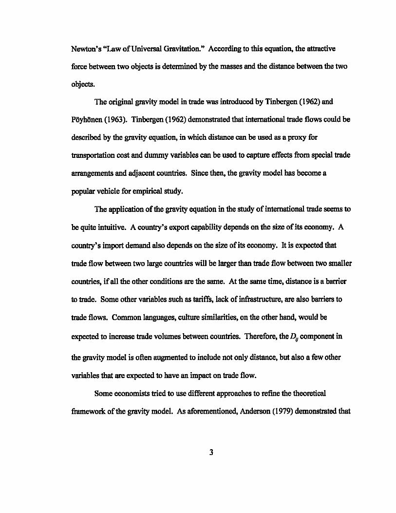
Newton's "Law of Universal Gravitation." According to this equation, the attractive

force between two objects is determined by the masses and the distance between the two

objects.

The original gravity model in trade was introduced by Tinbergen (1962) and

P6yhllnen (1963). Tinbergen (1962) demonstrated that international trade flows could be

described by the gravity equation, in which distance can be used as a proxy for

transportation cost and dummy variables can be used to capture effects from special trade

arrangements and adjacent countries. Since then, the gravity model has become a

popular vehicle for empirical study.

The application of the gravity equation in the study of international trade seems to

be quite intuitive. A country's export capability depends on the size ofits economy. A

country's import demand also depends on the size of its economy. It is expected that

trade flow between two large countries will be larger than trade flow between two smaller

countries, if all the other conditions are the same. At the same time, distance is a barrier

to trade. Some other variables such as tariffs, lack of infrastructure, are also barriers to

trade flows. Common languages, culture similarities, on the other hand, would be

expected to increase trade volumes between countries. Therefore, the Dy componeot in

the gravity model is often augmeoted to include not only distance, but also a few other

variables that are expected to have an impact on trade flow.

Some economists tried to use differeot approaches to refine the theoretical

framework of the gravity model. As aforemeotioned, Anderson (1979) demonstrated that

3

the gravity model can be derived from the pure expenditure system. He showed that a

simple gravity model is a rearrangement of a Cobb-Douglas expenditure function. In his

model. each country is completely specialized in producing one good and there is no

transport cost. Cobb-Douglas preferences are identical among the countries so that the

fraction of income spent on country i's product is the same in all countries. Anderson

(1979) stated that the expenditure model provides the functional form and most of the

explanatory power of the gravity model.

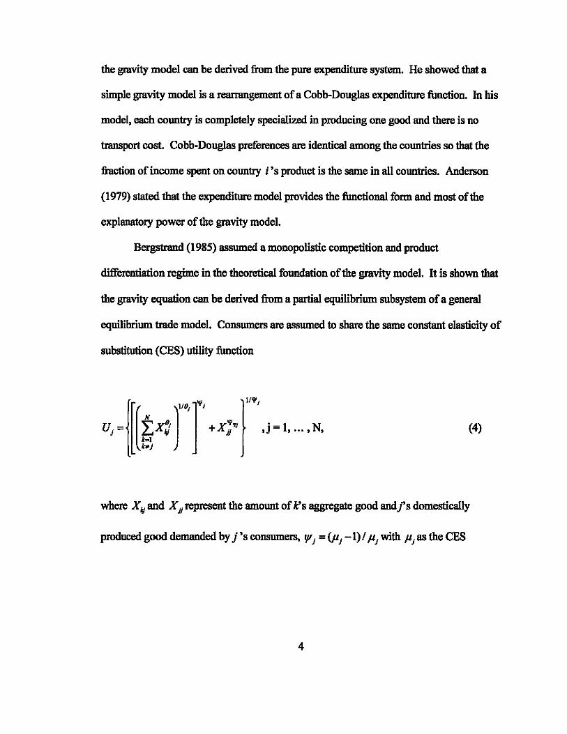
Bergstrand (1985) assumed a monopolistic competition and product

differentiation regime in the theoretical foundation of the gravity model. It is shown that

the gravity equation can be derived from a partial equilibrium subsystem of a general

equilibrium trade model. Consumers are assumed to share the same constant elasticity of

substitution (CBS) utility function

.j=I •...• N. (4)

where X Id and X D represent the amount of Ks aggregate good andfs domestically

produced good demanded by j's consumers. 'l'j =(Pj -1)/ Pj with pjas the CBS

4

between domestic and importable goods in}. 9J =(O'J -1)/ O'J with O'Jas the CBS among

importable goods in}.

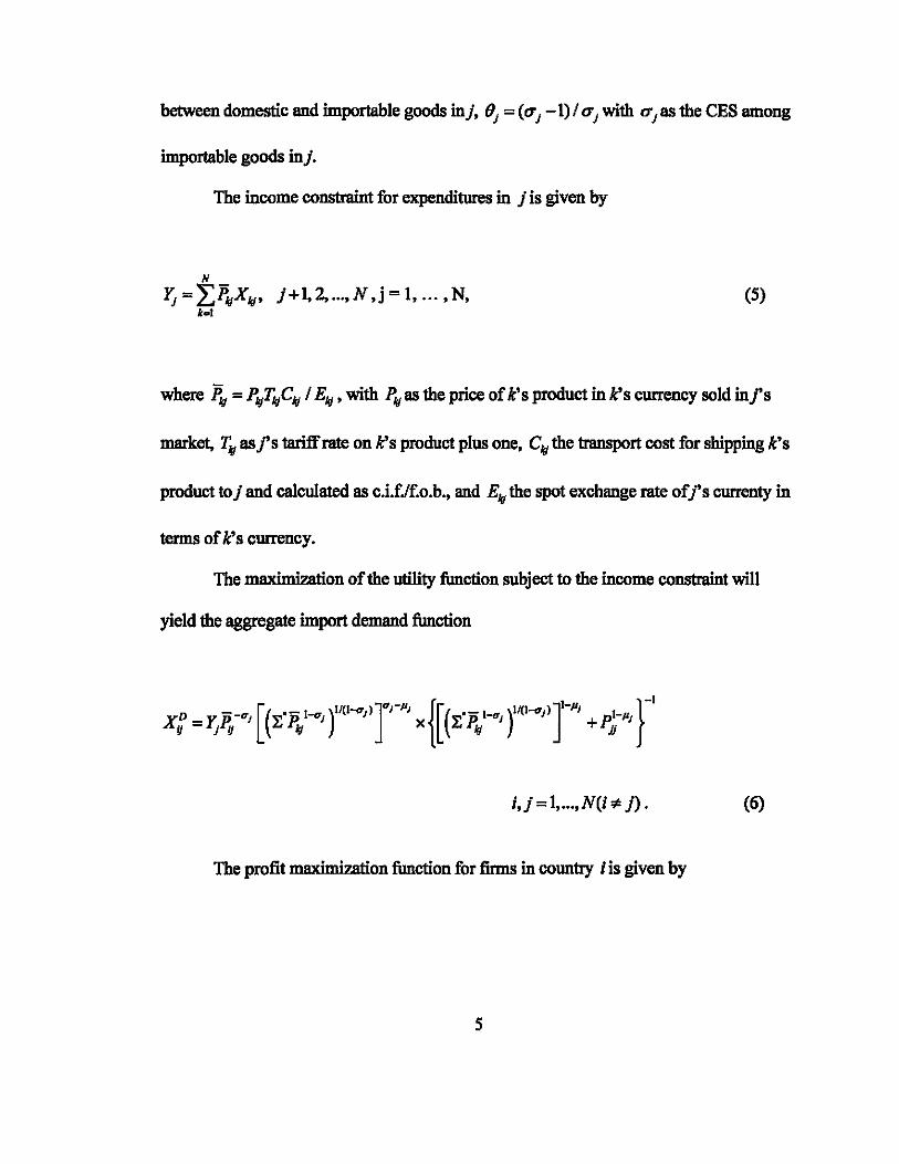
The income constraint for expenditures in } is given by

N

~=L~XIg' }+I.2, ...• N.j=I •...• N. (5) k.t

where ~ = PIgTIgCIg / Elg' with Pig as the price of k's product in k's currency sold in/s

market, TIg as/s tariffrate on k's product plus one. CIg the transport cost for shipping k's

product to} and calculated as c.i.fJf.o.b., and EIg the spot exchange rate of Is currenty in

terms of k's currency.

The maximization of the utility function subject to the income constraint will

yield the aggregate import demand function

i.} = 1 •...• N(i ¢ }) • (6)

The profit maximj7J!tion function for firms in country i is given by

s

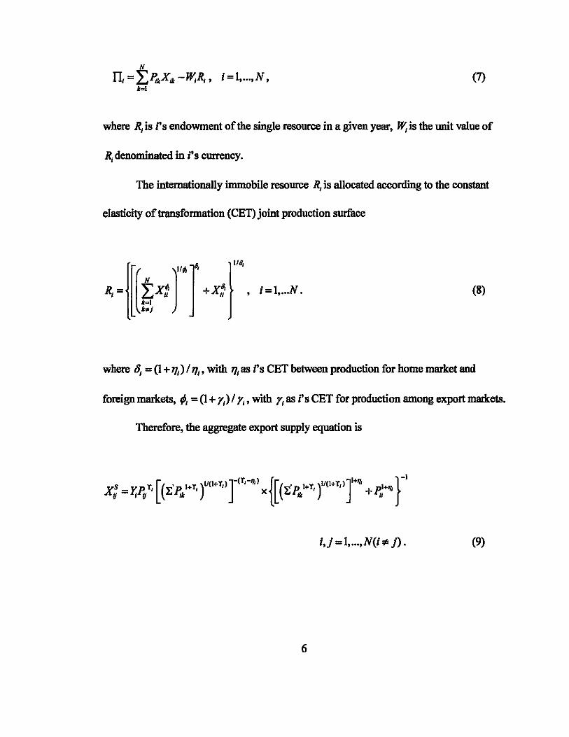
N

II, = LP/kX/k -w.R" i=I, ... ,N, (7) kQ(

where R, is i's endowment of the single resource in a given year, W. is the unit value of

R, denominated in i's currency.

The internationally immobile resource R, is allocated according to the constant

elasticity of transformation (CET) joint production surface

~ = [[~x: rr + x: ''', I=~ .. N (8)

where S. = (I + 'It) / 1f1' with 1f1 as i's CET between production for home market and

foreign markets, fA = (I + YI) / Y1 , with YI as i's CET for production among export markets.

Therefore, the aggregate export supply equation is

i,j = 1, ... ,N(1 ¢ j). (9)

6

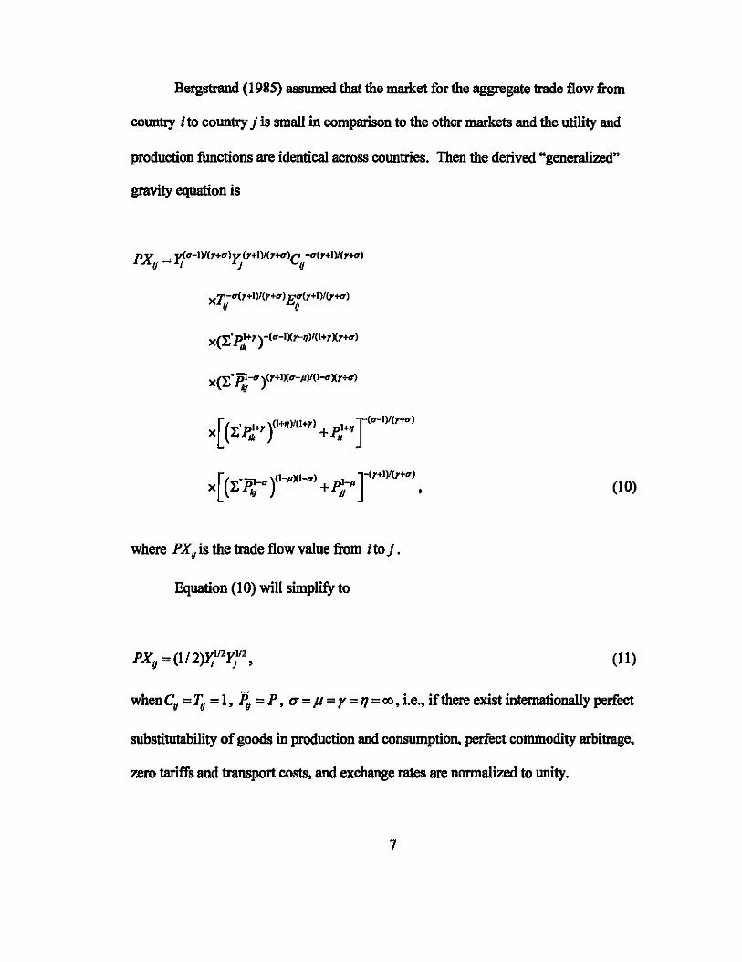
BeIgstllmd (1985) assumed that the marlcet for the aggregate trade flow from

country Ito country j is small in comparison to the other markets and the utility and

production functions are identical across COlDltries. Then the derived "generalized"

gravity equation is

xT.-u(r.I)/(y.CT) Eu(r+I)I(r.CT) If If

xCE'p~·r)-(CT-IXr-q)/(I.rxr ... )

x(E" ~ -cr )'r.1x tr-fl )I(I-cr Xr-)

X EP'+r +p'+q [( • 1 )(I+q)l(l+r) 1 J(tr-I)I(r+tr)

Ik u

[( "ii1-cr)(I-flXI-cr) l_fl]-(r+I)I(r+tr)

x EPo\'! +PD ' (10)

where PXg is the trade flow value from I to j .

Equation (10) will simplify to

(11)

when eg = 1U = 1, Py = P, u = J.l = r = T/ = co, i.e., if there exist internationally perfect

substitutability of goods in production and consumption, perfect commodity arbitrage,

zero tariffs and transport costs, and exchange rates are normalized to unity.

7

Bergstrand (1989) further considered the factor endowment, income and per

capital income variables in the gravity model. It combined the Hechscher-Ohin model

and the monopo1istically competitive model to derive a generalized gravity equation.

Deardorff (1998) established two different gravity models, one for "frictionless trade"

and the other for "impeded trade." As its name would suggest, the "frictionless trade"

model assumes away all transportation costs and other trade barriers. The "impeded

trade" model reintroduces transport costs into the equation.

In its empirical application, the gravity model is often used to study how transport

costs and trade costs affect trade. Transport costs historically exerted a large influence

over international trade, even though its importance has been declining over time

(Estevadeorclal et aI. 2003). But transport costs can still be economically significant for

some manufacturing industries. The transport costs of Japan's major manufacturing

firms accounted for 8.69 percent of their total sales value (Mori and Nishikimi 2002).

These firms also have to bear the time costs (interest costs) associated with the time spent

by goods in transit In addition, lower transport costs facilitate trade in indirect manners,

e.g., more frequent travel across borders increase bilatera1 trade flows (Gould 1994). It is

therefore necessary to understand how transport costs are determined and how transport

costs affect trade.

The concept of transport costs is important for economic studies. However,

spatial issues were avoided by economists for a long time (Siebert 1969). According to

8

Krugman (1991a, 1991b, 1995), mainstream economists neglected the economics of

space to avoid confronting the problem of market structure with increasing returns.

Trade costs are not limited to transport cost Trade costs include transport costs

(both freight costs and time costs), policy barriers (tariffs and non-tariff barriers),

infonnation costs, contract enforcement costs, costs associated with the use of different

currencies, legal and regulatory costs, and local distribution costs (wholesale and retail).

Anderson and Wincoop (2004) carried out a comprehensive survey of various aspects of

trade costs and concluded that trade costs are large. They asserted that trade barriers

dominate production costs, even though the latter have been the focus of most trade

theory. The pure international component of trade barriers, including transport costs and

border barriers but not local distribution margins, is estimated to be in the range of forty

to eighty percent for industrialized countries.

Hmnmels (1999) classified trade costs into three categories: explicit measured

costs (e.g., tariffs and freight rates), costs associated with common proxy variables such

as distance, sharing a language, sharing a border or being an island, and implied but

unmeasured trade costs, given by geographical position, cultural ties or political stability.

His results indicated that explicit measured costs were the most important component.

Differences in geographic location and access to water transportation can help to

explain differences in trade flows across countries. Baier and Bergstrand (2001) found

that falling transportation costs explain about eight percent of the average world trade

growth for several OECD countries since WWII. Raballand (2003) estimated the impact

9

of Iand-lockedness on trade for a panel database. Using a sample of 46 countries over a

five-year period and over 10,000 observations, he concluded that being landlocked would

reduce trade by more than eighty percent.

The negative impact of transport costs on trade is not limited to the landlocked

situation. Nicolini (2003) investigated regional trade flows between certain European

regions in a cross-section study and showed that physical distance reduces trading flows

while local transportation facilities as well as local demand increase them. Using data on

maritime and overland transport of products from the ceramic sector (tiles), Martinez­

Zarzoso et al. (2003) estimated a transport cost function to study the relationship between

transport costs and trade. Their results showed that higher transport costs significantly

reduce trade. Hummels (2001) suggested that, to some extent, import choices are made

in order to minimize transport costs.

Transport costs also depend on the weight, value, and consistency of goods.

Rauch (1999) divided production into homogeneous, near-homogeneous, and

differentiated goods. He showed that the insurance and freight costs as a percentage of

the total value are about twice as high for homogeneous and near-homogeneous goods

than for differentiated goods. Limao and Venables (2001) emphasized the role that

infrastructure plays in determining the cost of trade. A deterioration of infrastructure

from the median to the 75th percentile of destinations raises transport costs by twelve

percent. At the same time, the e1asticity of trade volume with respect to transport costs is

large. A ten percent increase in transport costs reduces trade volume by twenty percent.

10

Using transport costs data from five Latin-American countries, Martfnez-Zarzoso

(2002) estimated a transportation cost function to explore the determinants of transport

costs and the relationship between trade and transport. He showed that importer and

exporter income variables have a positive influence in bilateral trade flows, while

distance and poor infrastructure notably increase transport costs. He estimated the trade

elasticity with respect to transport costs to be 2.29.

One main obstacle in these studies is the difficulties in obtaining reliable data.

There are direct and indirect methods for obtaining data. Obtaining data from industry

associations or shipping firms is direct acquisition. Limao and Venables (2001) obtained

quotes from shipping firms for a standard container shipped from Baltimore to various

destinations. Hummels (2001) used indices of ocean shipping from trade journals and

air-freight rates from survey data. Direct methods are not always feasible due to data

limitations and the large size of the resulting datasets.

Some countries and international organizations provide data on trade flows that

allow detailed unit values to be constructed indirectly. For example, the U.S. Census

reports U.S. imports valued at f.o.b. and c.i.f. bases. Researchers can get a unit value

estimate of bilateral transport cost from this dataset Hummels (2001) made use of this

method for data from the U.S.A., New Zealand and five Latin-American countries.

Harrigan (1993) and Baier and Bergstrand (2001) used the aggregate bilateral c.i.fJf.o.b.

ratios produced by the IMP. Since most importing countries report c.i.f. trade flows and

11

exporting countries report f.o.b. trade flows, transport costs can be estimated as the

difference of both flows for the same aggregate trade.

Limao and Venables (2001) provided a revised version of the transport costs

model. The authors showed that the transport costs for commodity Ie, shipped between

countries i and}, can be written as

TCllk = F(X4 Xi. VII. eIj) , (12)

where Xi and Xi are country-specific characteristics, e.g., geographical and infrastructure

measures; VII is a vector of characteristics relating to the shipping condition between t

and} , e.g., distance between trading countries, volume of imports that go trough a

particular route, and dummy variables for common language and common border; and eIj

represents unobservable variables.

A simplified transport cost function in the multiplicative form is

where TCllk denotes freight ad-valorem rates, with t as the importer country,} the exporter

country and k the commodity. DII denotes distance. Islandl and IslandJ are dummy

variables that take the value of one when the importer or the exporter is an island, zero

12

otherwise. Landlockedl and Landlockec(j are dummy variables used to describe if

importer and exporter are landlocked or not Languageqtakes the value of one when

cOImtries i and} speak a common language, zero otherwise. Colony takes the value of

one if the trading countries had a colonial relationship. The error term is assumed to be

independently and identically distributed.

The general specification in log form is

InTCUk =~ inDy +azlsland, +a3Island}, +a.Land,

+asLand} + a 6Lang + a,Conoly + 8U' (14)

After a discussion of the determinants of transport costs, the question is then how

much transport costs affect trade volume. The gravity model is the main device that has

been used to link trade barriers to trade volume. In Limao and Venables (2001), the

volume of imports (exports) between pairs of countries, Mq, is a function of their incomes

(GDPs), transport costs and a set of dummies and can be expressed as

(15)

where y, and ~represent GDPs of the exporting country and importing country

respectively, rCq measures the transport costs between the two countries, and 11/1 is the

13

error term. Trade is expected to be positively related to economic mass and negatively

related to transport costs.

A log-linear transformation of equation (15) is

(16)

Substituting equation (14) for transport cost, equation (16) becomes an augmented

gravity equation relating trade to distance and other variables,

InMu = Po + P.lnJ; + P21n~ + A inDy + Pislandj + PsIslandJ

+ P6Lantij + P7LandJ + p7Lang + PgCO/ony + By (17)

This is the typical econometric version of the gravity model in the existing trade

literature. Even though this model has been generally quite successful, the following

section will demonstrate that it may have misspecification problems due to several factors.

14

1.3 Misspeeifications

The original gravity equation is

(18)

where q is the gravitation constant, m, and m J are mass of object i and object J. and

dq is the distance between them. The counterpart of the gravity equation in international

trade may be expressed as

(19)

where Vq measures bilateral trade volume between countries I and J, y, is the GDP of

country i. YJ

is the GDP of country j. and dq are variables that measure trade-resisting

factors including geographical as well as non-geographical factors such as cultural and

legal dissimilarities.

A possible misspecification in the gravity model is the choice of the dependent

variable. In the original gravity equation. the force is bidirectional rather than

unidirectional and its primary detenninjng factor is the product of two masses or

composite mass~11Ia in Equation (18). To stay within this framework, the trade volume

15

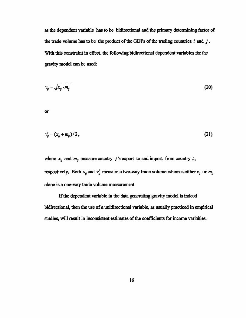
as the dependent variable has to be bidirectional and the primary determining factor of

the trade volume has to be the product of the ODPs of the trading countries i and j.

With this constraint in effect, the following bidirectional dependent variables for the

gravity model can be used:

(20)

or

(21)

where Xu and mu measure country j's export to and import from country i.

respectively. Both vuand v~ measure a two-way trade volume whereas either Xu or my

alone is a one-way trade volume measurement

If the dependent variable in the data generating gravity model is indeed

bidirectional, then the use of a unidirectional variable, as usually practiced in empirical

studies, will result in inconsistent estimates of the coefficients for income variables.

16

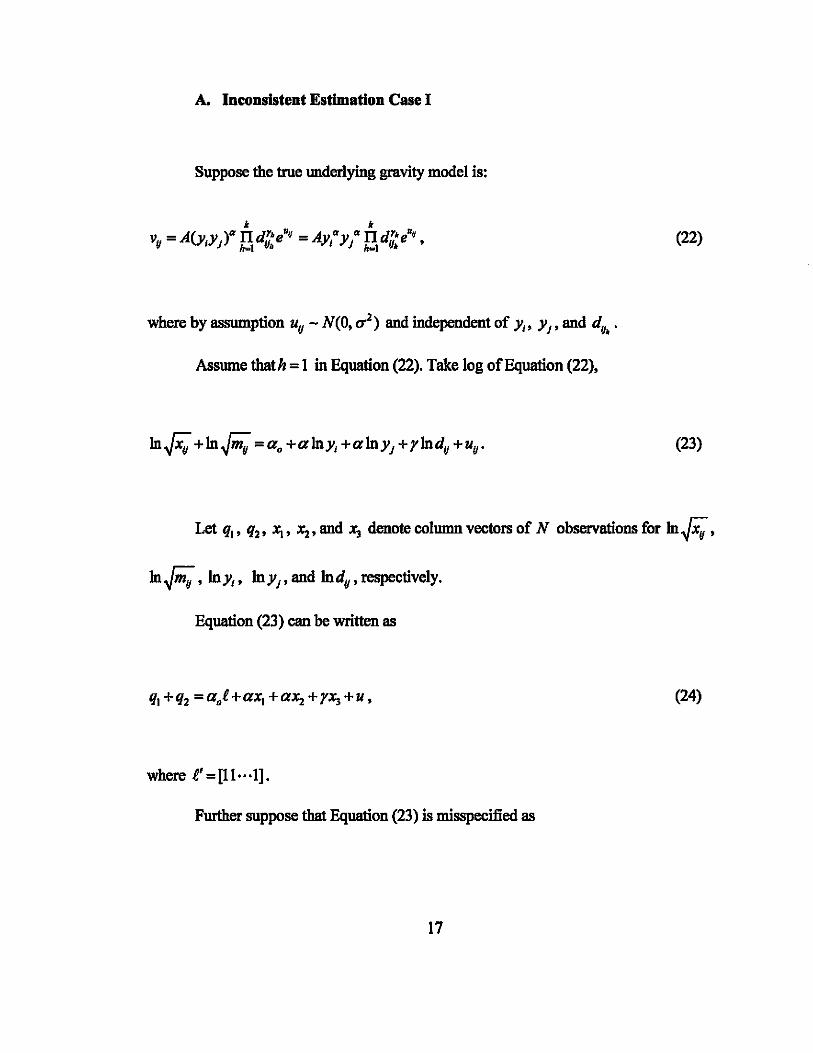
A. Inconsistent Estimation Case I

Suppose the true underlying gravity model is:

k k

A'" )a ITd"·u A a a ITd" Uu v" = V'IYj "e = Jil Yj "e, tI' h .. t Vb /tal Vi

(22)

where by assumption UIJ - N(O, 0'2) and independent of YI' Yj' and dlJ ••

Assume thath = 1 in Equation (22). Take log of Equation (22),

(23)

Let q .. Q2' Xt, ~. and ~ denote column vectors of N observations for In,Ji; ,

Equation (23) can be written as

(24)

where £'=[11 .. ·1].

Further suppose that Equation (23) is misspecified as

17

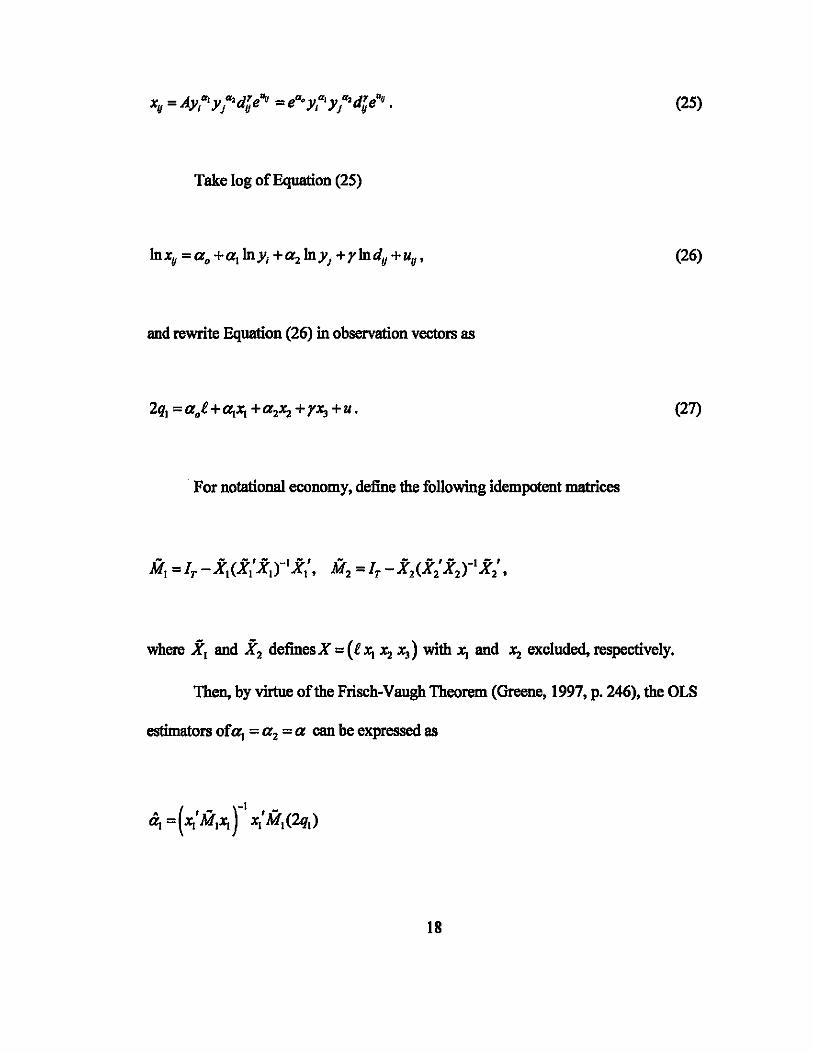
(25)

Take log of Equation (25)

(26)

and rewrite Equation (26) in observation vectors as

(27)

For notational economy, define the following idempotent matrices

where Xl and X2 definesX=(l.li.l2 Xl) with.li and .l2 excluded, respectively.

Then, by virtue of the Frisch-Vaugh Theorem (Greene, 1997, p. 246), the OLS

estimators of~ = a2 = a can be expressed as

18

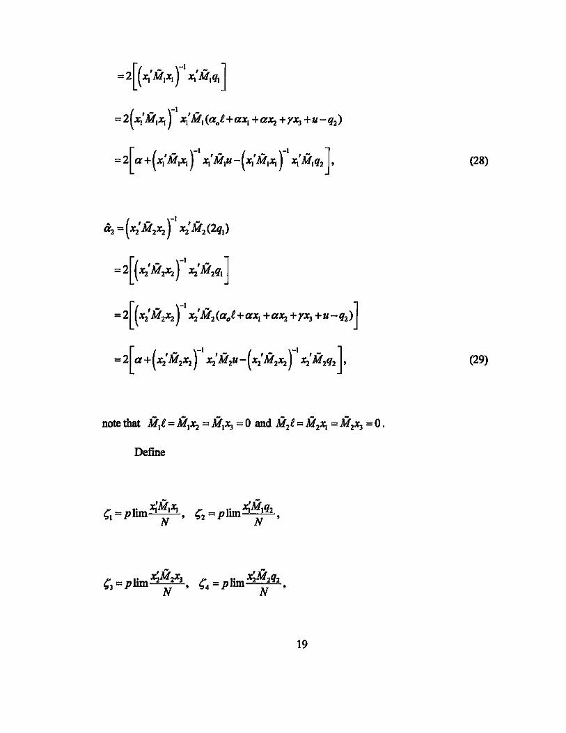
(28)

(29)

Define

19

(30)

(31)

note that Uy is by assumption independent of all regressors, by the law of large numbers,

estimators ofa. Further, unless(2 / ~ = (4 / (3' which is unlikely either,

20

B. Inconsistent Estimation Case n

Suppose the data generating process for the gravity model is:

, -At,. )adT u. a.(y )ad T u. Vy - U'IYj Y e = e IYj Y e • (32)

Take log of Equation (32).

(33)

With q3 denoting the observation vector forln[(xy +my)/2]. the full model in

Equation (33) can be written as

Suppose Equation (33) is misspecified as

y _ A"a,y a'dTeu• ~y - >1'1 j Y , (34)

take log of Equation (34).

21

(35)

Equation (35) can be written as

(36)

Define fl as the colmnn vector for observationsfl, aln«(l+my / xy)/2). the OLS

estimators of a. and a2 can be expressed as

~ =(X/MI~ r ~'MI(2qI) =(x/MI~ r ~'MI (q3 -fl)

=a+(~'MI~ r ~'MIU-(~'MI~r ~'Mlfl.

el2 =(~'M2~ r ~'M2(2qI) =(~'M2~ r ~'M2(q3 -fl)

=a+(~'M2X2r ~'M2U-(~'M2~r ~'M2fl.

22

(37)

(38)

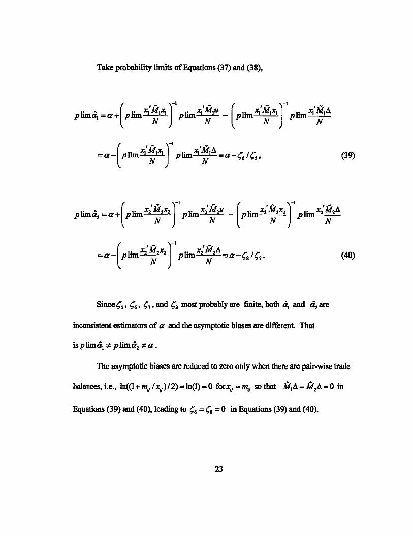
Take probability limits of Equations (37) and (38),

(39)

(40)

inconsistent estimators of a and the asymptotic biases are different. That

The asymptotic biases are reduced to zero only when there are pair-wise trade

Equations (39) and (40), leading to '6 = '8 = 0 in Equations (39) and (40).

23

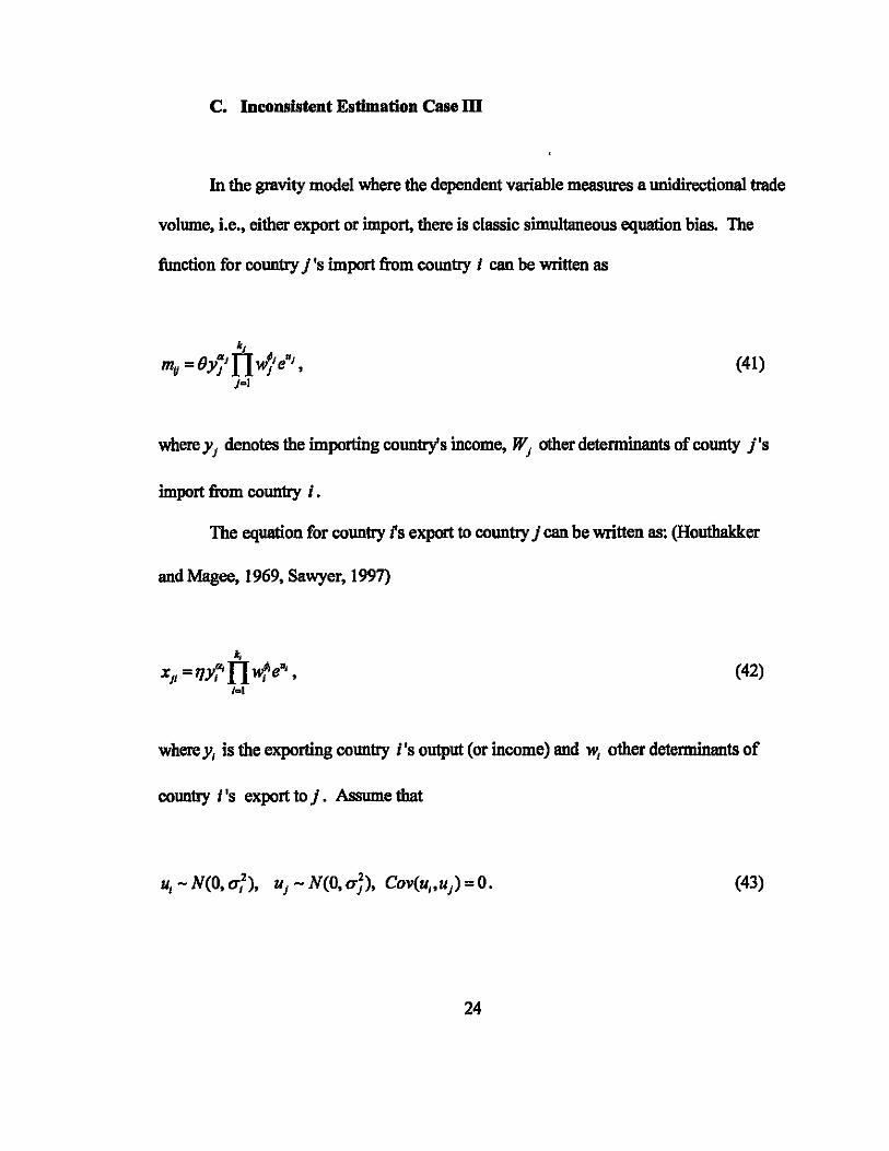
C. Inconsistent Estimation Case m

In the gravity model where the dependent variable measures a unidirectional trade

volume, i.e., either export or import, there is classic simultaneous equation bias. The

function for country j 's import from country i can be written as

(41)

where Yj denotes the importing country's income, Wj other determinants of county j's

import from country i.

The equation for country fs export to country j can be written as: (Houthakker

and Magee, 1969, Sawyer, 1997)

(42)

where YI is the exporting country i's output (or income) and WI other determinants of

country i's export to j. Assume that

(43)

24

Multiply the corresponding sides of Equations (41) and (42), then reflect the

(44)

take square root of both sides of Equation (44),

(45)

which is the gravity model.

Take the log of both sides of Equation (45),

It, k

+L9V2lnw,+ I:¢/2lnwj +(u,+u}12 , j

(46)

However, in Equation (46) both y, and Yj are correlated with fly due to the

identity:my = xJI'

Equate log of Equations (41) and (42), and write In y, and In YJ as

25

It is clear from Equation (47) that E(ullnYI)=-u! lal ¢O and

E(uj lny) = -u;, I a j ¢ O. Therefore, the OLS estimators of fJ. and fJ2 in the gravity

model in Equation (46) are inconsistent

1.4 Simulation Analysis

The previous section has shown that the identity of country i 's import from

country j with county j 's export to country i could cause a serious simultaneous

equation bias. Furthermore, the coefficient estimates for the real ODPs of destination and

originating countries in the gravity model are expected to be only half of the value of

their counterparts in the export and import equations.

An interesting observation in trade literature is that the estimatOO coefficients for

real ODP variables in the gravity model are no less in magnitude and sometimes even

26

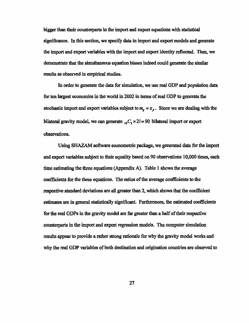
bigger than their counterparts in the import and export equations with statistical

significance. In this section, we specify data in import and export models and generate

the import and export variables with the import and export identity reflected. Then, we

demonstrate that the simultaneous equation biases indeed could generate the similar

results as observed in empirical studies.

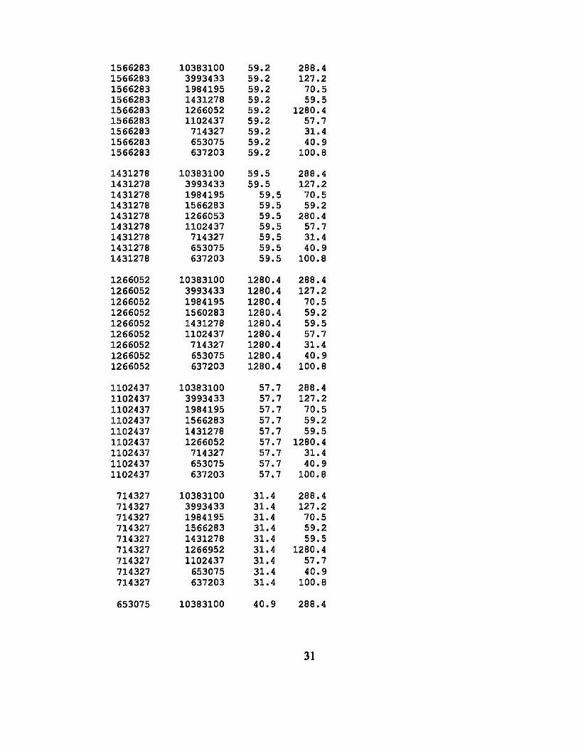
In order to generate the data for simulation, we use real GOP and population data

for ten largest economies in the world in 2002 in terms of real GOP to generate the

stochastic import and export variables subject to mil = XJI • Since we are dealing with the

bilateral gravity model, we can generate 10 C2 X 21 = 90 bilateral import or export

observations.

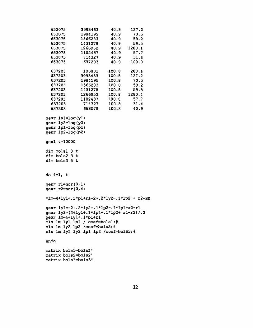
Using SHAZAM software econometric package, we generated data for the import

and export variables subject to their equality based on 90 observations 10,000 times, each

time estimating the three equations (Appendix A). Table 1 shows the average

coefficients for the three equations. The ratios of the average coefficients to the

respective standard deviations are all greater than 2, which shows that the coefficient

estimates are in general statistically significant Furthermore, the estimated coefficients

for the real OOPs in the gravity model are far greater than a half of their respective

countetparts in the import and export regression models. The computer simulation

results appear to provide a rather strong rationale for why the gravity model works and

why the real GOP variables of both destination and origination countries are observed to

27

have as strong effects on the bilateral trade between the countries as when they appear

separately in import and export models.

Table 1. Averages of 10,000 Coefficient Estimates

Equation I: Import Equation

Coefficient Meatl standardDev . . .

Maximl,Jln mmunum

y, 0.96301 0.39301 -0.56542 2.4351

pop, 31.873 0.19740 30.377 33.155

consl -121.19 0.92402 -127.64 -114.65

Equation II: Export Equation

• Coefficient Mean standard Dev . minimum Maximum

YJ 2.2526 0.52499 0.29389 4.0424

pOPJ -4.1951 0.23306 -5.7495 -2.6510

consJ 12.358 7.0419 -11.992 40.821

Equation m: Gravity Model

Coefficient Mean standard Dev minimum Maximum

y, 0.94476 0.39890 -0.62111 2.4038

YJ 2.4303 0.26262 0.58634 4.2974

pop, 31.888 0.20052 30.419 33.252

pOPJ -0.67167 0.21189 -2.0671 0.59840

cons -152.68 3.5771 -178.78 -127.62

28

1.5 Conelusion

This essay explores some existing problems associated with the gravity model in

terms of estimation bias. In particular, this essay explains why the gravity model works

in general, i.e., why the impact ofreal ODPs of both importing and exporting countries in

the gravity model always matter. This phenomenon is caused by simultaneous equation

biases, which is further proved by the simulation results. Another issue may well be how

to eliminate those biases off the gravity model, which is beyond the scope of this essay.

29

Appendix A

The Monte Carlo Programs

(Using the Shazam econometric package)

* GDP and population for ten largest economies of the world in 2002 were used to generate other variables for Monte Carlo experiments.

set ranseed=1000000 set noecho

sample 1 90 read y1 y2 pI p2

10383100 3993433 288.4 127.2 10383100 1984195 288.4 70.5 10383100 1566283 288.4 59.2 10383100 1431278 288.4 59.5 10383100 1266052 288.4 1280.4 10383100 1102437 288.4 57.7 10383100 714227 288.4 31.4 10383100 653075 288.4 40.9 10383100 637203 288.4 100.8

3993433 10383100 127.2 288.4 3993433 1984195 127.5 70.5 3993433 1566283 127.5 59.2 3993433 1431278 127.5 59.5 3993433 1266052 127.5 1280.4 3993433 1102437 127.5 57.7 3993433 714327 127.5 31.4 3993433 653075 127.5 40.9 3993433 637203 127.5 100.8

1984195 10383100 70.5 288.4 1984195 3993433 70.5 127.5 1984195 1566283 70.5 59.2 1984195 1431278 70.5 59.5 1984195 1266052 70.5 1280.4 1984195 1102437 70.5 57.7 1984195 714327 70.5 31.4 1984195 653075 70.5 40.9 1984195 637203 70.5 100.8

30

1566283 10383100 59.2 288.4 1566283 3993433 59.2 127.2 1566283 1984195 59.2 70.5 1566283 1431278 59.2 59.5 1566283 1266052 59.2 1280.4 1566283 1102437 59.2 57.7 1566283 714327 59.2 31.4 1566283 653075 59.2 40.9 1566283 637203 59.2 100.8

1431278 10383100 59.5 288.4 1431278 3993433 59.5 127.2 1431278 1984195 59.5 70.5 1431278 1566283 59.5 59.2 1431278 1266053 59.5 280.4 1431278 1102437 59.5 57.7 1431278 714327 59.5 31.4 1431278 653075 59.5 40.9 1431278 637203 59.5 100.8

1266052 10383100 1280.4 288.4 1266052 3993433 1280.4 127.2 1266052 1984195 1280.4 70.5 1266052 1560283 1280.4 59.2 1266052 1431278 1280.4 59.5 1266052 1102437 1280.4 57.7 1266052 714327 1280.4 31.4 1266052 653075 1280.4 40.9 1266052 637203 1280.4 100.8

1102437 10383100 57.7 288.4 1102437 3993433 57.7 127.2 1102437 1984195 57.7 70.5 1102437 1566283 57.7 59.2 1102437 1431278 57.7 59.5 1102437 1266052 57.7 1280.4 1102437 714327 57.7 31.4 1102437 653075 57.7 40.9 1102437 637203 57.7 100.8

714327 10383100 31.4 288.4 714327 3993433 31.4 127.2 714327 1984195 31.4 70.5 714327 1566283 31.4 59.2 714327 1431278 31.4 59.5 714327 1266952 31.4 1280.4 714327 1102437 31.4 57.7 714327 653075 31.4 40.9 714327 637203 31.4 100.8

653075 10383100 40.9 288.4

31

653075 3993433 653075 1984195 653075 1566283 653075 1431278 653075 1266952 653075 1102437 653075 714327 653075 637203

637203 103831 637203 3993433 637203 1984195 637203 1566283 637203 1431278 637203 1266952 637203 1102437 637203 714327 637203 653075

genr ly1=10g(y1) genr ly2=10g(y2) genr lp1=log(p1) genr lp2=10g(p2)

gen1 t=10000

dim bolsl 3 t dim bols2 3 t dim bols3 5 t

do 11=1, t

genr r1=nor(0,1) genr r2=nor(0,4)

40.9 127.2 40.9 70.5 40.9 59.2 40.9 59.5 40.9 1280.4 40.9 57.7 40.9 31.4 40.9 100.8

100.8 288.4 100.8 127.2 100.8 70.5 100.8 59.2 100.8 59.5 100.8 1280.4 100.8 57.7 100.8 31.4 100.8 40.9

*lm=4+1y1+.1*pl+r1=2+.2*ly2-.1*lp2 + r2=EX

genr ly1=-2+.2*ly2-.1*lp2-.1*lp1+r2-r1 genr ly2=(2+ly1+.1*lp1+.1*lp2+ rl-r2)/.2 genr 1m=4+ly1+.1*p1+r1 ols 1m ly1 lp1 / coef=bols1:i ols 1m ly2 lp2 /coef=bols2:# ols 1m ly1 ly2 Ip1 lp2 /coef=bols3:#

endo

matrix bols1=bols1' matrix bols2=bols2' matrix bols3=bols3'

32

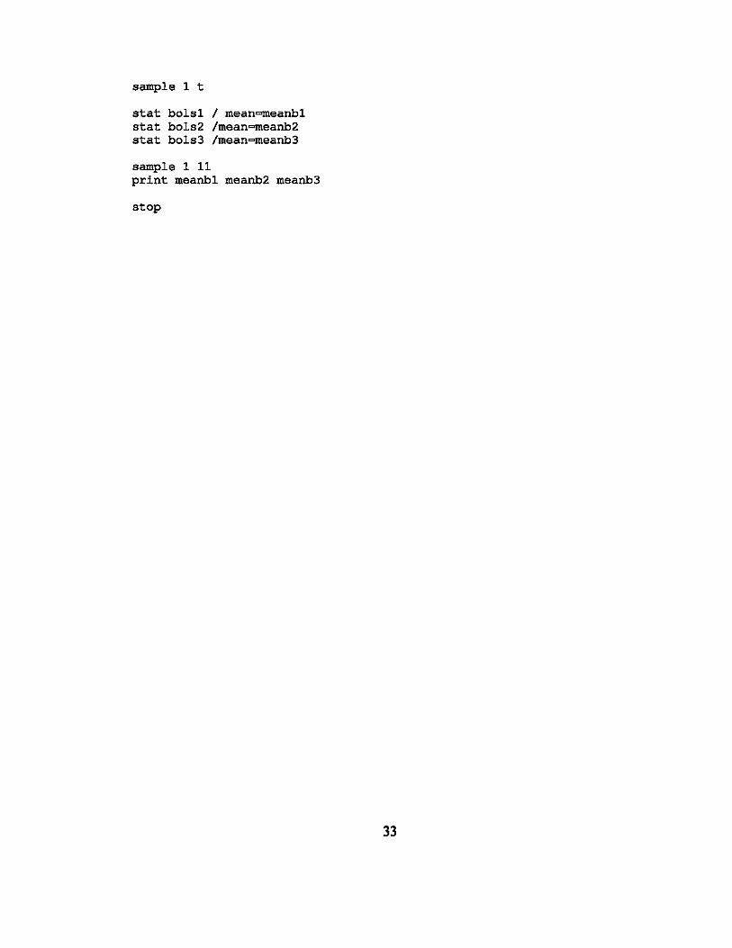
sample 1 t

stat bolsl I mean=meanbl stat bols2 Imean=meanb2 stat bols3 Imean=meanb3

sample 1 11 print meanbl meanb2 meanb3

stop

33

References

Anderson, J. E. (1979) "A Theoretical Foundation for the Gravity Equation," American Economic Review, Vol. 69, I, 106-16.

Anderson, J. E., E. von Wincoop (2003) "Gravity with Gravitas: A Solution to the Border Puzzle," American Economic Review, Vol. 43, , 170-92.

Anderson, J.E., E. von Wmcoop (2004) "Trade Costs," Journal o/Economic Literature, 42(3),691-751.

Baier, S. L., J. H. Bergstrand (2001) "The Growth of World Trade: Tariffs, Transportation Costs, and Income Similarity," Journal o/Internotionol Economics, 53(1), 1-27.

Bergstrand, J. H. (1985) ''The Gravity Equation in International Trade: Some Microeconomic Foundations and Empirical Evidence," Review 0/ Economics and Statistics, 67(3), 474-81.

Bergstrand, J. H. (1989) "The Generalized Gravity Equation, Monopolistic Competition, and the Factor-Proportions Theory in International Trade," Review o/Economics and Statistics, 71(1),143-53.

Cheng, I., H. Wall, (2005) "Controlling for Heterogeneity in Gravity Models of Trade and Integration," Federal Reserve Bank St. Louis Review, 87(1),49-63.

Deardorff, A. V. (1998) "Determinants of Bilateral Trade: Does Gravity Work in a Neoclassical World?" in THE REGIONALIZA TION OF THE WORLD ECONOMY (Frankel, J. A., ed.).

Donald, D., D. Weinstein (1996) "Does Economic Geography Matters for International Specialisation?" NBER Working Paper 5706.

Egger, P., M. Pfaffermayr (2003) "The Proper Panel Econometric Specification of the Gravity Model: a Three-Way Model with Bilateral Integration Effects," Empirical Economics, 28, 571-80.

Estevadeordal, A., Frantz, B., A. M. Taylor (2003) "The Rise and Fall of World Trade, 1870-1939," Quarterly Journal o/Economics, 118 (2), 359-407.

34

Fratianni, M., H. Kang (2006) "Heterogeneous Distance-Elasticities in Trade Gravity Model," Economics Letters, 90, 68-71.

Glaeser, E. L., J. E. Koblhase (2003) "Cities, Regions and the Decline of Transportation Costs," NBER Working Paper 9886.

Gould. D. M. (1994) "Immigration Link to the Home Country: Empirical Implications for U.S. Bi1ateraI Trade Flows," The Review o/Economics and Statistics, 76, 302-16.

Greene, W. H. (1997) ECONOMETRIC ANALYSIS (3rd ed.), Prentice Hall, New Jersey.

Harrigan, J. (1993) "OECD Imports and Trade Barriers in 1983," JouranI of International Economics, 35, 91-111.

Helpman, E. (1987) "Imperfect Competition and International Trade: Evidence from Fourteen Industrial Countries," J01l17ll1l o/the Japanese and International Economies, 1(1),62-81.

Henderson, J. V., Shalizi, Z., A. J. Venables (2001) "Geography and Development," Journal o/Economic Geography, 1,81-106.

Houtbakker, H. S., S. P. Magee, 1969, "Income and Price Elasticities in World Trade," The Review 0/ Economics in World Trade, LI (2), 111-25.

Hummels, D. (1999) "Towards a Geography of Trade Costs," mimeo.

Hummels, D. (2001) "Have International Transportation Costs DeclinedT' J01l17ll1l 0/ International Economics, 54 (I), 75-96.

Jones, vi J., E. Berglas (1977) "Import Demand and Export Supply: An Aggregation Theorem," American Economic Review, 67(2), 183-7.

Justman, M. (1994) "The Effect ofLoca1 Demand on Industry Location," The Review 0/ Economics and Statistics, 76(4), 742-53.

Knlgman, P. (1991a) GEOGRAPHY AND TRADE, MIT Press.

Knlgman, P. (1991b) "Increasing Returns and Economic Geography," Journal 0/ Political Economy, 99 (3), 483-99.

Kmgman, P. (1995) DEVELOPMENT, GEOGRAPHY, AND ECONOMIC THEORY.

35

Leamer, E. E., R. M. Stern (1970) QUANTITATIVE INTERNATIONAL ECONOMICS, Aleline Publishing Company, Chicago.

Limao, N., A. J. Venables (2001) "Infrastructure, Geographical Disadvantage and Transport Costs," World Bank Economic Review, 15 (3), 451-79.

Markusen. J., A. J. Venables (1996) "The Theory of Endowment, Intra-Industry and Multinational Trade," NBER Working Paper 5529.

Martfnez-Zarzoso, I. (2002) "T}.'atlSportation Costs and Trade: Empirical Evidence for LatinoAmerican Imports from the European Union," mimeo.

Martinez-Zarzoso, I. (2003) "Gravity Model: An Application to Trade between Regional Blocks," Atlantic Economic Journal, 31 (2), 174-87.

Matyas. L. (1997) "Proper Econometric Specification of the Gravity Model," The World Economy, 20, 363-9.

Martinez-Zarzoso, I., Garcia-Menendez, L., C. Suarez-Burguet (2003) "Impact of Transportation Costs on International Trade: The Case of Spanish Ceramic Exports," Maritime Economics and Logistics, 5(2), 179-98.

Morl, T., K. Nishikimi (2002) "Economies ofTransportation Density and Industrial Agglomeration," Regional Science and Urban Economics, 32, 167-200.

Nicolini, R. (2003) "On the Determinants of Regional Trade Flows," International Regional Science Review, 26(4), 447-65.

Nozick, L. K., M. A. Turnquist (2001) "Inventory, Transportation, Service Quality and the Location of Distribution Centers," European Journal of Operational Research, 129(2),362-71.

Oguledo, V.I., C. R. Macphee (1994) "Gravity Models: A Reformulation and an Application to Discriminatory Trade Arrangements," Applied Economics, 26, 107-120.

PlIyh1lnen, P. (1963) "A Tentative Model for the Vohnne ofTrade between Countries," Weltwirtschqftliches Archlv, 90, 93-9.

36

Raballand, G. (2003) "Determinants of the Negative Impact of Being Landlocked on Trade: An Empirical Investigation through the Central Asian Case," Comparative Economic Studies, 45(4), 520-36.

Rauch, J. E. (1999) "Networks Versus Markets in International Trade." Journal of International Economics, 48, 7-35.

Roberts, B. A. (2004) "A Gravity Study of the Proposed China-ASEAN Free Trade Area," International Trade Journal, XVIII (4), 335-53.

Sawyer, W. C. (1997) "Communication: The Demand for Imports and Exports in Japan: A Survey,· Journal of the Japanese and International Economics, 11,247-59.

Saxonhouse, G.R. (1989) "Differentiated Products, Economies of Scale, and Access in the Japanese Market," in TRADE POLICIES FOR INTERNATIONAL COMPETITIVENESS (Freenstra, R. C., ed.), University of Chicago Press for NBER, 145-74.

Siehert H. (1969) REGIONAL ECONOMIC GROwm, THEORY AND POLICY, International Textbook Company, Scranton, USA.

Tinbergen, J. (1962) "An Analysis of World Trade Flows," in SHAPING THE WORLD EcONOMY (Tinbergen, J. ed.). The Twentieth Centwy Fund, New York.

Venables, A. (2001) "Geography and International Inequalities: The Impact of New Technologies," Journal of Industry , Competition and Trade, 1(2), 135-59.

Venables, A., N. Limao (2002) "Geographical Disadvantage: a Heckscher-Ohlin-Von­Tunen Model of International Specialization," Journal of International Economics, 58(2), 239-63.

Yamarik S., S. Ghosh, (2005) "A Sensitivity Analysis of the Gravity Model," The International Trade Journal, XIX (1), 83-126.

37

Essay Two

An Alternative Approach to the Co-integration Test

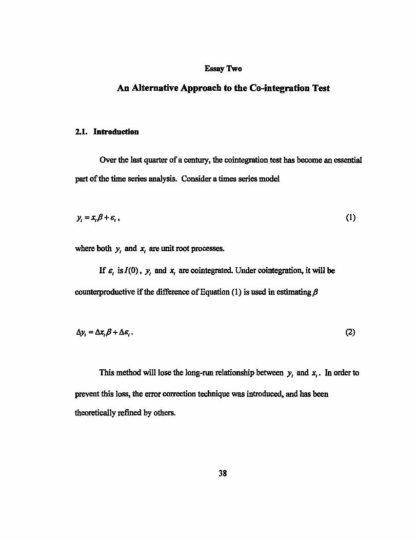
2.1. Introduetion

Over the last quarter of a century, the cointegration test has become an essential

part of the time series analysis. Consider a times series model

where both y, and x, are unit root processes.

If s, is 1(0), y, and x, are cointegrated. Under cointegration, it will be

counterproductive if the difference of Equation (1) is used in estimatingp

Ay, = Ax,P + As,.

(1)

(2)

This method will lose the long-run relationship between y, and x,. In order to

prevent this loss, the error correction technique was introduced, and has been

theoretically refined by others.

38

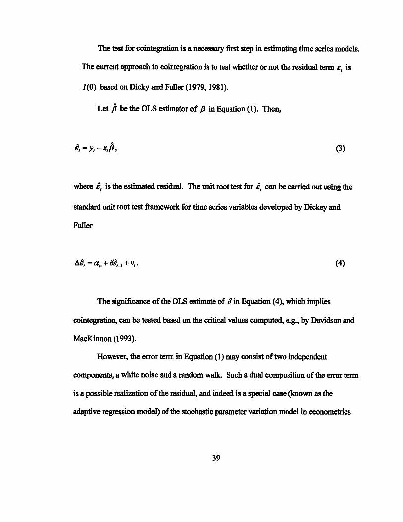
The test for cointegration is a necessary first step in estimating time series models.

The current approach to cointegration is to test whether or not the residual term s, is

1(0) based on Dicky and Fuller (1979,1981).

Let P be the OLS estimator of P in Equation (1). Then,

8,=y,-X,p, (3)

where 8, is the estimated residual. The unit root test for 8, can be carried out using the

standard unit root test framework for time series variables developed by Dickey and

Fuller

(4)

The significance of the OLS estimate of 0 in Equation (4), which implies

cointegration, can be tested based on the critical values computed, e.g., by Davidson and

MacKinnon (1993).

However, the error term in Equation (1) may consist of two independent

components, a white noise and a random walk. Such a dual composition of the error term

is a possible realization of the residual, and indeed is a special case (known as the

adaptive regression model) of the stochastic parameter variation model in econometrics

39

literature. If the true realization of the residual is dual, then the Dickey-Fuller unit root

test framework in Equation (4) will be a misspecification, rendering the test results

invalid.

This essay is organized as follows. Section 2.2 is the literature review. Section

2.3 introduces the adaptive regression model. Section 2.4 explores the range and

distribution of g. Section 2.5 offers an alternative cointegration test. Section 2.6 is the

simulation analysis. The last section concludes.

2.2. Literature Review

One important aspect of time series models is the methodology through which the

stochastic process is incorporated into the model. In a typical stochastic process, it is

assumed that eachYl.Y2 .... J;.in the series is a random value from a probability

distribution. The representation of this randomness is the core of the modeling. The

predicting power of the model depends on how the probability distribution function is

specified. Since it is generally impossible to specifY this function completely. a

simplified model is often used in its place to approximate the actual distribution.

It is not always justifiable to assume that the process is stationary. A process is

stationary if it is invariant with respect to time. If the process changes over time. it is

nonstationary. According to Kennedy (1992). for a long time. econometricians simply

40

asswned that economic data are stationary. They were primarily concerned about issues

such as autocorrelated errors and simultaneity. However, the nonstationarity could cause

many problems in data analysis because of the stochastic nature of a series.

A mndom walk process is an example of such stochastic model. Pindyck and

Rubinfeld (1998) offered a straightforward and useful illustration of this process, in

which y, is determined by

y, = Y,-l +s" (5)

where E(s,) = o and E(s,ss) = o when I,#s.

The expected values for y in the following periods will be

(6)

However, the error variance and the standard error of forecast will increase with the

forecast periodl and the error variance becomes lu.2 •

Many macroeconomic variables follow mndom walk, e.g., consumption follows a

rsndom walk. Hall (1978) was the first author to state that consumer nondurable goods

follow an autoregressive process of order one, an AR(J). In his famous mndom walk

model, he predicted that the dependent variable in the current period depends on its past

41

value and a stochastic error term. If the lagged dependent variable has a unit root, then

the process is nonstationary.

Mankiw (1982) applied Hall's framework to durable goods, which has a

depreciation rate less than one. Based on the foundation of Hall (1978)'s optimization

framework, he showed consumer durables expenditures display an ARMA(1,1) process.

The empirical results give Mankiw an autoregressive process, an AR(1), instead. This

implies that data analysis yields a random walk process for durable expenditure as well.

Hansen and Singleton (1983) showed that nondurable goods in log-linear form

also follow a random walk. Mankiw (1985) employed a Taylor series approximation to

obtain a log linear model for consumer durables as a function of consumer nondurables.

He points out that if the log of consumer nondurables follows a random walk as shown in

Hansen and Singleton (1983), then the log of consumer durables also follows a random

walk. Romer (2001) analyzed the stock of consumer durables and concluded that the

stock of consumer durables follows a random walk.

In the random walk model, ifupward or downward trend is taken into

consideration. then we will get what is called a random walk with drift. It is represented

by:

y, =Y'-1 +d+s,. (7)

42

In this case, for d > 0, both the forecasts and the standard error of forecast will increase

with I.

On the other hand, if the stochastic process is

Y,=&" (8)

and &, is an independently distributed random variable with zero mean, this process is

referred to as white noise. The forecast will be YT., = 0 •

Time series analysts use differencing methods to deal with the stationarity

problem. Box and Jenkins (1970) proposed what would become known as the ARlMA

(p,d,q) or n Auto-Regressive Integrated Moving Average" models. In this model, p is the

number of autoregressive terms, d is the number of nonseasonal differences, and q is the

number oflagged forecast errors in the prediction equation (moving average terms). The

lags of the differenced series and lags of the forecast errors are added to the model

specification to remove autocorrelation problems from the forecast errors. Through

differencing and logging, the series become stationarized. Random-walk models,

random-trend models, and autoregressive models are all special cases of ARlMA models.

The Box-Jenkins process creates a new data series, Y,* and

(9)

43

where thee are independently and identically distributed normal errors with zero mean.

The methodology used in the single variable Box-Jenkins model can also be

extended to multivariate Box-Jenkins model, where ARIMA process is chosen for an

entire vector of variables. On the other hand, the structural econometric time series

approach (SEMTSA) is based on the theory that multivariate time series processes are

genera1izations of the dynamic structural equation econometric models. Despite the fact

that ARIMA models out-forecast the traditional method, many econometricians do not

want to give up their traditional structural modeling since the ARIMA models do not

explain how the economy works.

The error-correctlon model (ECM) is a major step forward for the

econometricians. A simple example of this model can be expressed as

where y andx are expressed in logarithms. Since economic theory demands that

(10)

y and x will grow at the same rate in the long run. we can set y, = Y,_I , and x, = X,_I. It

can be derived that f3.. + P2 + P2 = 1.

We can also get

(11)

44

which is the ECM expression with the error-correction term. If the level variables

y and x are indeed integrated of order one, (Yt-l - X'_l) is integrated of order zero.

If the series ifnot stationary, the Box-Jenkins is not valid. However, Box and.

Jenkins used differencing to remove any nonstationarity. Econometricians

underestimated the detrimental effect of nonstationarity until it is proven that traditional

t and DW statistics will not work with nonstationary data. Through a Monte Carlo

experiment, Granger and Newbold (1974) discovered that conventional significance test

tends to accept a spurious relationship when researchers fail to consider the existence of

stochastic trends in time series data. Phillips (1986) provided a rigorous proof for their

discoveries.

In the last few decades, researchers have considered different types of regression

and different types of data generating process. Many researchers focused on the linear

specification. The most prominent ones include the driftless random walks in Granger

and Newbold (1974) and Phillips (1986), two independent random walks with non-zero

drifts in Entorf(1997), 1(2) processes in Haldrup (1994), nonstationary

fractionally integrated processes in Marmol (1998), and stochastic unit root processes in

Granger and Swanson (1997).

Some researchers also considered the possibility of spurious nonlinear

relationship, such as Lee et al. (2005). Using both finite sample and large sample, their

45

paper showed that spurious nonlinear regressions can occur in nonlinear estimation where

two independent random wa1ks are used.

Phillips (1986, 1987) is a pioneer in the establishment of asymptotic theory for

regressions with stochastic trends. Phillips and Durlauf (1986) extended this approach to

the multivariate setting. The asymptotic methods provided by these authors have served

as main tool to derive most of the limit results in the context of unit root nonstationarity.

Instead of being satisfied with just removing trends by differencing in univariate

time series modeling, researchers turned to focus on the autoregressive (AR) unit roots

and the development of statistical procedures to detect them. Dickey and Fuller (1979)

and Fuller (1976) were among the first in developing the most popular tests for unit roots.

They tabulated special critical values for the t statistics in the unit root test. Guilkey and

Schmidt (1989) and Schmidt (1990) also tabulated these special critical values for

different sample sizes and special cases.

In the error-correction models mentioned above, if the level data are 1(1), the

ECM equation will not generate the right results. Only if the combination of these level

data are 1(0), ECM equation will not generate spurious results. Kennedy (1992)

recommended the following methodology for econometricians. First, find out the order

of integration of the raw data series by using unit root tests. Second, run cointegration

regression and test for cointegration by using unit root tests. Third, use an ECM if

cointegration is accepted.

46

However, none of the existing paper has studied the cointegration test statistics in

the context of the adaptive regression model. Since the Dickey-Fuller unit root test

framework will not function in such a specification, the test results are invalid. Therefore,

this paper will attempt to develop new test statistics for the adaptive regression model.

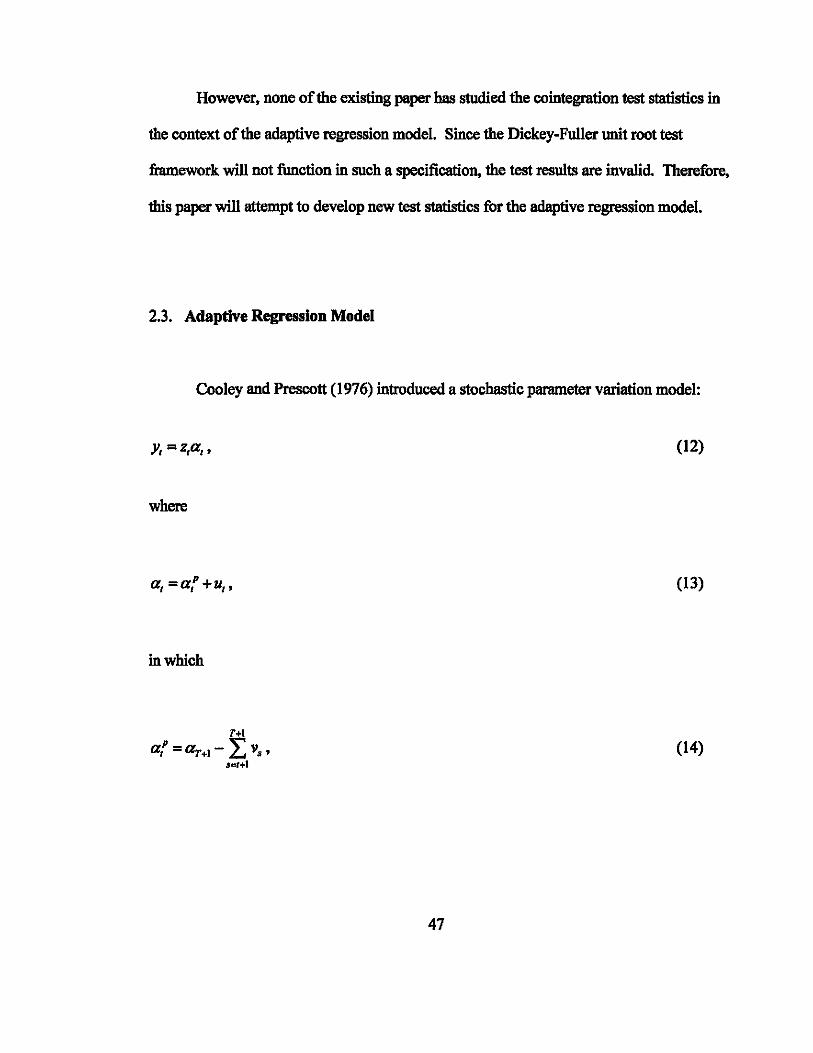
2.3. Adaptive Regression Model

Cooley and Prescott (1976) introduced a stochastic parameter variation model:

y, =z,a"

where

a, =ai+u"

in which

T+l

a'p =aT+1 - L Va' Sat+.

(12)

(13)

(14)

47

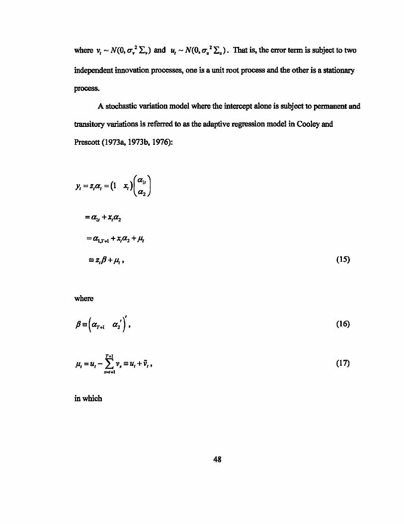
where v, - N(O, 0'.2 ~.) and u, - N(O, 0'.2 ~.). That is, the error term is subject to two

independent innovation processes, one is a unit root process and the other is a stationary

process.

A stochastic variation model where the intercept alone is subject to permanent and

transitory variations is referred to as the adaptive regression model in Cooley and

Prescott (1973a, I973b, 1976):

Y, =z,a, =(1 XI >(::)

az,fi+p"

where

T.l

P, =u, - LV. au, +;;" 8.,+1

in which

(15)

(16)

(17)

48

scr (r Min(T -i+l.T- j+l) + (l-r». (i.j = 1.2 •..•• T) (18)

where

(19)

In term of matrices

y=ZP+P. (20)

where

(21)

(22)

49

T T-l 2 1

T-l T-l ... 2

Q= 1

2 2 1

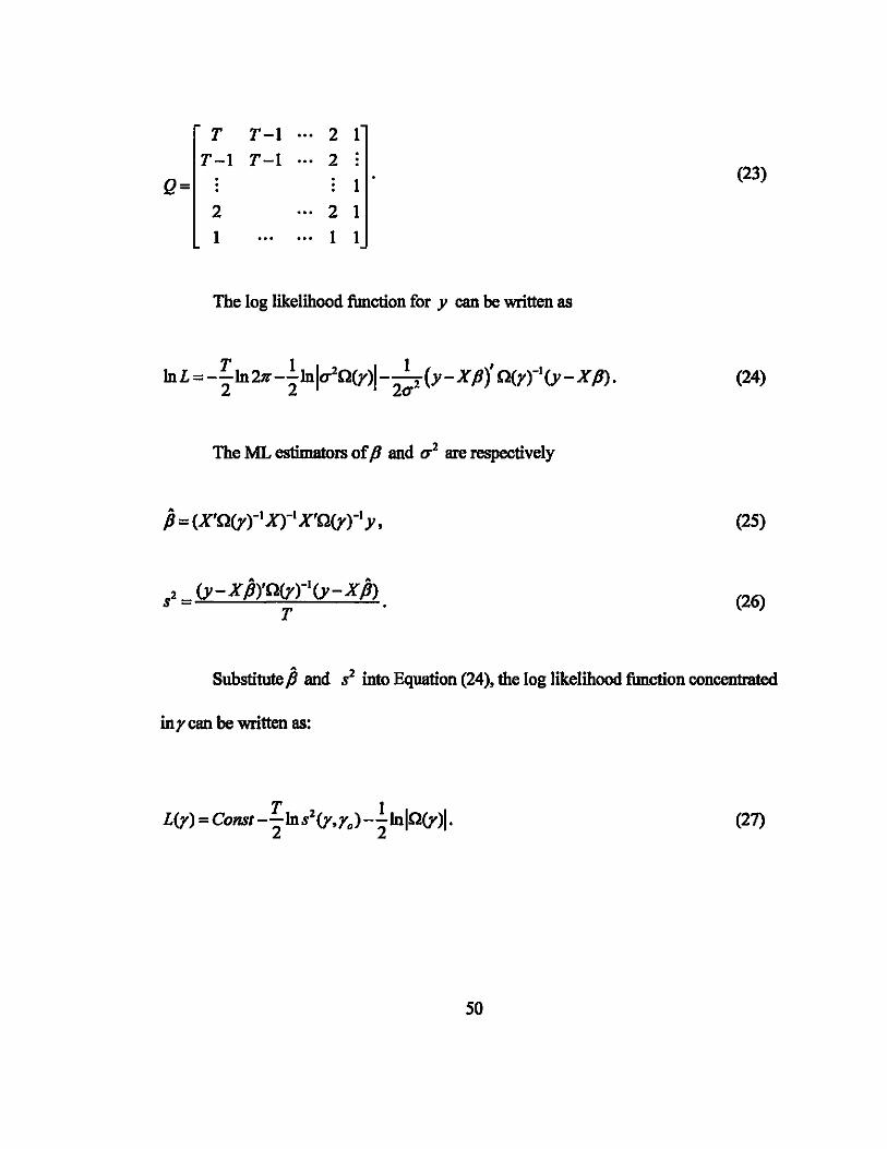
1 1 1

The log likelihood fimction for y can be written as

T 1 1_2 1 1 ( )' -I lnL=--ln211'--ln u-O(y) -- y-XfJ O(r) (y-XfJ). 2 2 2u2

The ML estimators of fJ and u 2 are respectively

?- (y-XP)'O(Yfl(y-XP) T

(23)

(24)

(25)

(26)

Substitute P and 82 into Equation (24), the log likelihood fimction concentrated

inrcan be written as:

T 1 L(y) = Const --ln82(Y,r.)--lnl0(Y)I.

2 2 (27)

50

For analytical ease, Q(y) is diagona1ized by premultiplying C to y=ZP+ f.l

where C is such that CC' = e'c = IT and C'QC = D. C is the matrix whose columns are

the characteristic vectors of Q, and D is the diagonal matrix of characteristic roots of Q.

d _ 1 , !ft(t) n(T-t+l) I 4cos2 !ft(/) 2T + 1

(28)

For economies of notations, Cy, CX , and C f.l are written as y, X, and f.l

respectively. Then

(29)

(30)

dl 0 0 0

0 d2 0

D= 0 0 (31)

0 dT

_1 0

0 0 dT

51

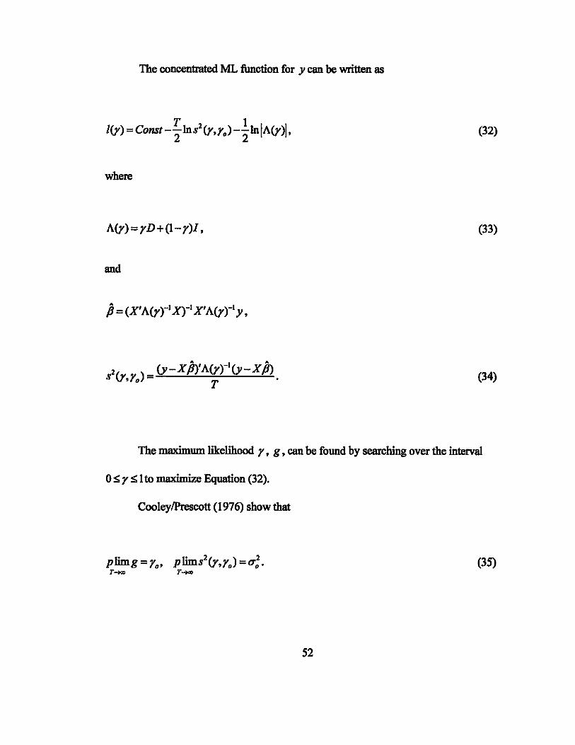
The concentrated ML function for y can be written as

(32)

where

A(Y)=rD+(I-r)I, (33)

and

P = (X'A(Yrl X)-I X'A(rrl y,

(34)

The maximum likelihood r, g, can be found by searching over the interval

OS r S 1 to maximize Equation (32).

CooleylPrescott (1976) show that

plimg=r., plims2(Y,r.) =0';. (35) T-')(1J T~

52

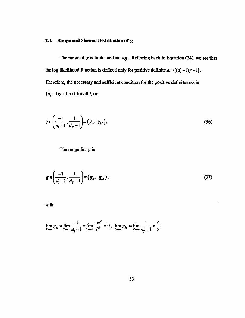
2.4. Range and Skewed Distribution of g

The range of r is finite, and so is g. Referring back to Equation (24), we see that

the log likelihood function is defined only for positive definite A = [(dt -I)y+ 1].

Therefore, the necessary and sufficient condition for the positive definiteness is

(d, -1)r + 1> 0 for all t, or

(36)

The range for g is

(37)

with

S3

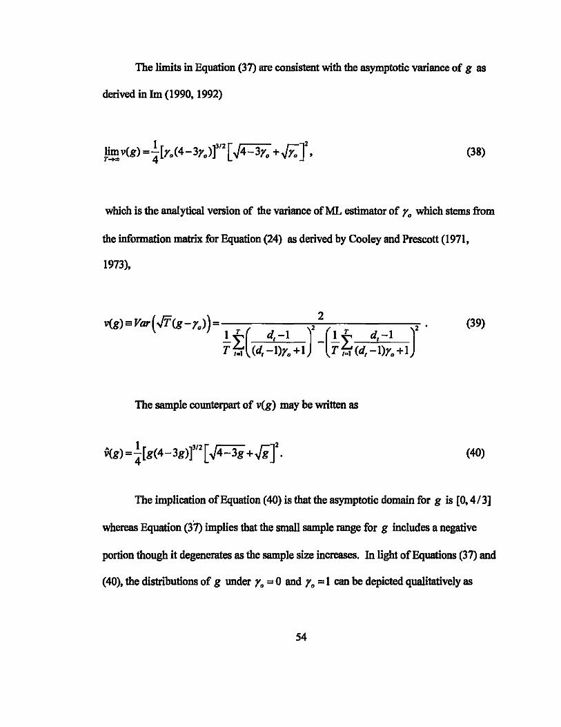
The limits in Equation (37) are consistent with the asymptotic variance of g as

derived in 1m (1990,1992)

Iimv(g) =.!.[r.(4-3r.)f/2[~4-3r. +Ji;]2. T_ 4

(38)

which is the analytical version of the variance ofML estimator of r. which stems from

the information matrix for Equation (24) as derived by Cooley and Prescott (1971,

1973),

v(g) a Var(.JT"(g-r.») = 2 2 2 • (39) It( d,-I ) (It d,-I ) T to\ (d, -I)r. +1 T M (d,-I)r. +1

The sample counterpart of v(g) may be written as

v(g) = ![g(4-3g)t[ ~4-3g+~r. (40)

The implication of Equation (40) is that the asymptotic domain for g is [0,4/3]

whereas Equation (37) implies that the smaIl sample range for g includes a negative

portion though it degenerates as the sample size increases. In light of Equations (37) and

(40), the distributions of g under r. = 0 and r. = 1 can be depicted qualitatively as

54

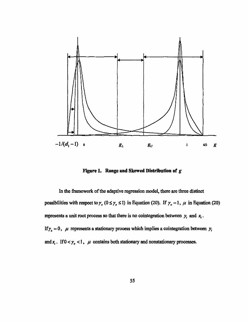
-1/(d. -1) 0 gu 413 g

Figure 1. Range and Skewed Distribution of g

In the framework of the adaptive regression model, there are three distinct

possibilities with respect to Yo (0 s Yo S 1) in Equation (20). If Yo = 1, II in Equation (20)

represents a unit root process so that there is no cointegration between y, and x,.

Ifro = 0, II represents a stationary process which implies a cointegration between y,

andx,. If 0 < ro <1, II contains both stationary and nonstationary processes.

55

The significance of the analytical expression in Equation (38) is that the variance

of g is zero, which violates the conditions in the Central Limit Theorem, therefore the

probability distribution ofg is non-normal. Han (1997) computationally confirmed the

non-normality of g. However, an exact distribution formula for g has not been

introduced in econometric literature. The following section will introduce analytical test

statistics for H. : r. = 0 and H. : r. = 1.

2.5. Alternative Test Statistics

The first order condition for maximizing

(41)

can be written as

(42)

where

56

P=(X'A<rflX)-IX'A<rrly,

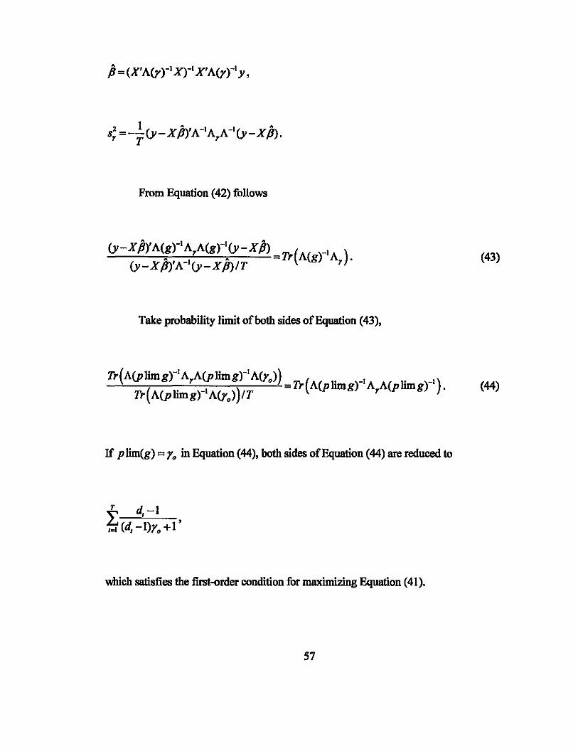
From Equation (42) follows

(y- X PY A(grl A,A(grl(y- X iJ)

(y-XP)'A-I(y-XiJ)IT

Take probability limit of both sides of Equation (43),

(43)

Tr(A(pJim rIA A( Jim rIA(~») g ,P g Vo =Tr(A(p1im )-IA A(plim )-1). (44)

Tr(A(plimgfIA<ro»)IT g, g

If plim(g) ='0 in Equation (44), both sides of Equation (44) are reduced to

± d,-I , ,al (d, -1)'0 + 1

which satisfies the first-order condition for maximizing Equation (41).

57

Since L17 (r) < 0 (See Appendix B for proof), g is a unique consistent estimator

of Yo'

Now define a new statistic q:r :

Equation (45) can be written in terms of scalars as

T f.. p")2 T "2 L v,-X, L Il,

( ) _ Icl (d, -I)yo + 1 _ ,=1 (d, -I)yo + 1

q:r g,yo - 1 T (y, -x,Pi -1.. T p,2 Tt;:(d,-I)g+1 Tt;:(d,-I)g+1

Since

pJimg=yo'

(d, -I)yo +1 -+ [(d, -I)yo + 1]8,2 82

T__ (d,-I)Yo+1 '

58

(45)

(46)

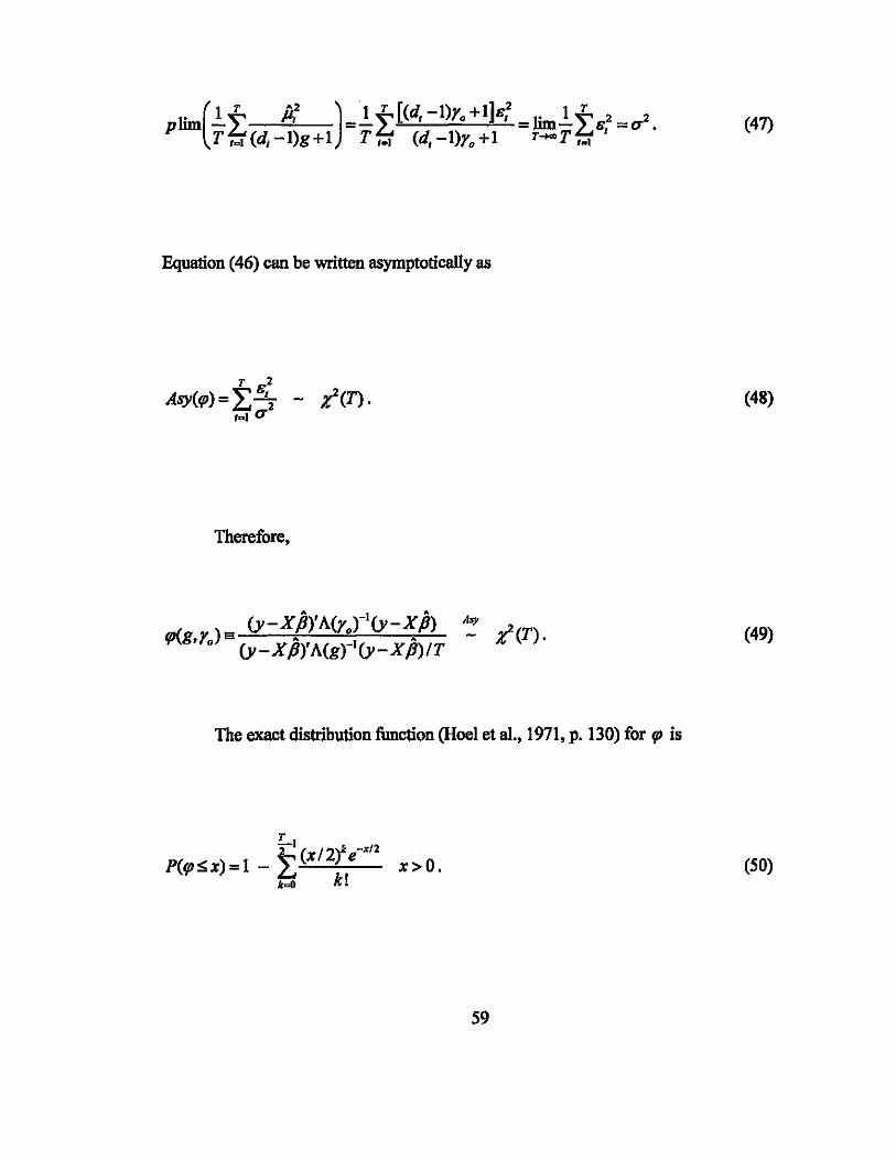
Equation (46) can be written asymptotically as

(48)

Therefore,

(49)

The exact distribution function (Hoet et aI., 1971, p. 130) for rp is

(SO)

59

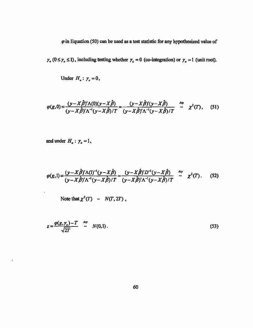
rp in Equation (SO) can be used as a test statistic for any hypothesized value of

r. (0 S r. S 1), including testing whether r. = 0 (co-integration) or r. = 1 (unit root).

Under H.: r. =0,

and under H.: r. =1,

NotetbatZ2 (T) - N(T,2T),

rp(g,r.)-T A.\Y N(O 1) z .J2T - ,. (53)

60

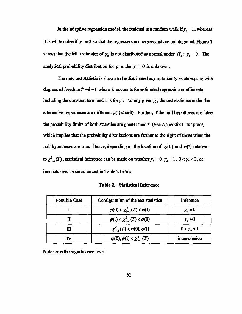
In the adaptive regression model, the residual is a random walk if r. = I, whereas

it is white noise if r. = 0 so that the regressors and regressand are cointegrated. Figure 1

shows that the ML estimator of r. is not distributed as normal under H.: r. = O. The

analytical probability distribution for g under r. = 0 is unknown.

The new test statistic is shown to be distributed asymptotically as chi-square with

degrees of freedomT - k -1 where k accounts for estimated regression coefficients

including the constant term and 1 is for g. For any given g , the test statistics under the

alternative hypotheses are different: 9'(1) ¢ 9'(0). Further, if the null hypotheses are false,

the probability limits of both statistics are greater thanT (See Appendix C for proof),

which implies that the probability distributions are farther to the right of those when the

null hypotheses are true. Hence, depending on the location of 9'(0) and qJ(l) relative

to zt-«(T) , statistical inference can be made on whether r. = 0 ,r. = I, 0 < r. < I, or

inconclusive, as summarized in Table 2 below

Table 2. Statistical Inference

Possible Case Configuration of the test statistics Inference

I 9'(0) < Zl:a (T) < 9'(1) r. =0

II 9'(1) < Z't-a(T) < 9'(0) r. =1

m Zl:a (T) < 9'(0), 9'(1) O<r. <1

IV 9'(0),9'(1) < Zl:a(T) inconclusive

Note: a is the significance level.

61

2.6. Simulation Analysis

The maximum likelihood estimator of the instability parameter r. is not normally

distributed. In addition, under the null r. = 0, the ML estimator of r. converges to

r. = 0 with the order ofO(T2). Therefore, we expect tbat the normalized Chi-squares do

not degenerate to zero or explode as T increase. This section will show how the

normalized Chi-squares statistic for g, the ML estimator ofr., behaves under

H. : r. = O. To make it as simple as possible without loss of generality, we generated the

dependent variable as N(O, 1) process under r. = O. Hence, the normalized Chi-square

test statistic can be expressed as

(54)

where g denotes r such tbat

T 1 1(g):1:1(y)=Cons--lns2(Y)--ID(Y)1 V r.

2 2 (55)

62

We iterated the data generation and grid search for g over r E [-lI(d\ -1).1] 100

times for different sample sizestif E [1,100] (Appendix E). Since the lower bound for g

rapidly approach 0 from below, r was increased at an increasing rate lIS it approaches.

Table 3 shows how the critical points for four different levels of cumulative probabilities

vary lIS the degrees of freedom increase given the number of iteration at 100. There is no

sign for either convergence to zero or divergence to infinity, which implies that the

critical points are finite.

Though 98% confidence level of the statistic defined by [ 10\' ~99] is a bit

volatile, 95% confidence level defined by [ ~05'~9S] is relatively stable. There may be

two reasons for this observation. First, the left tail of the probability distribution is

extremely thin so that the left-hand critical point is extremely sensitive to a slight shift of

the probability mass either to the left or to the right. Second. the number of iterations is

rather small. This appears to be apparent from Table 4 which shows more stable critical

points for N=l 000 for a selected number of sample sizes.

As the sample size increases, the probability distribution becomes smoother lIS we

compare Figure 2 for N=500 and Figure 3 for N=IOOO.

63

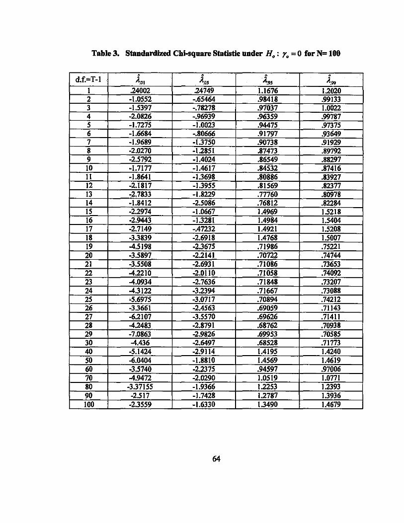
Table 3. Standardized Chi-square Statistic under H.: Y. = 0 for N= 100

d.f.=T·l I 2

4

I

13 .4

·1.53

·1.72 .11; .1

·2. 0 .; .

·2.1817 ·2.7833

95

.247'19 76 R

·.78278

.1

.

.882' • il~ .874 .L'169! .83927

.82377 .77760

_" ,0<; 76R 2

19 4.5198 ·2.3675 .71986 ., 5221 20 .; ;.5897 .221.41 .7072 47'

~-2~ill~~--~,~~,~~nR--~--~~~~6~+---~--~.771~10~8---+---~.,J~6~--~ 22 ,_221n ·2.0110 .7105 .740! 2: .(~'l.4 .~ 7636 .71848 .732' 2 ~In ''l~ '166' .na 2: .: ,975 .: 171' 1089< _742 21 1661 L~6' .on~4 .711' 27 ·6.2107_ ·3.5571 0<;00<;", .71411 28 ...d "AR~ .2.8791 O<;R70<;" .70938 29 .7_nIl61 .2,91126 o<;oo,,~ .. 585 30 4 .26< Q7 0<;' 'R "~I

41 ·5. ·2.9: I' 51 ..r. ·1.81 H 1.- i9 61 ·3.5740 ·2.237~ .9701 71 -'1.9<172 -" ,on 1.0519 1.0771 81 ·3 37155 .1 166 1 "~1 1.2393 91 ·2.5 17 .1. 12~ 1.2781 1.3936 100 ·2.3559 .161'1n 1.4679

64

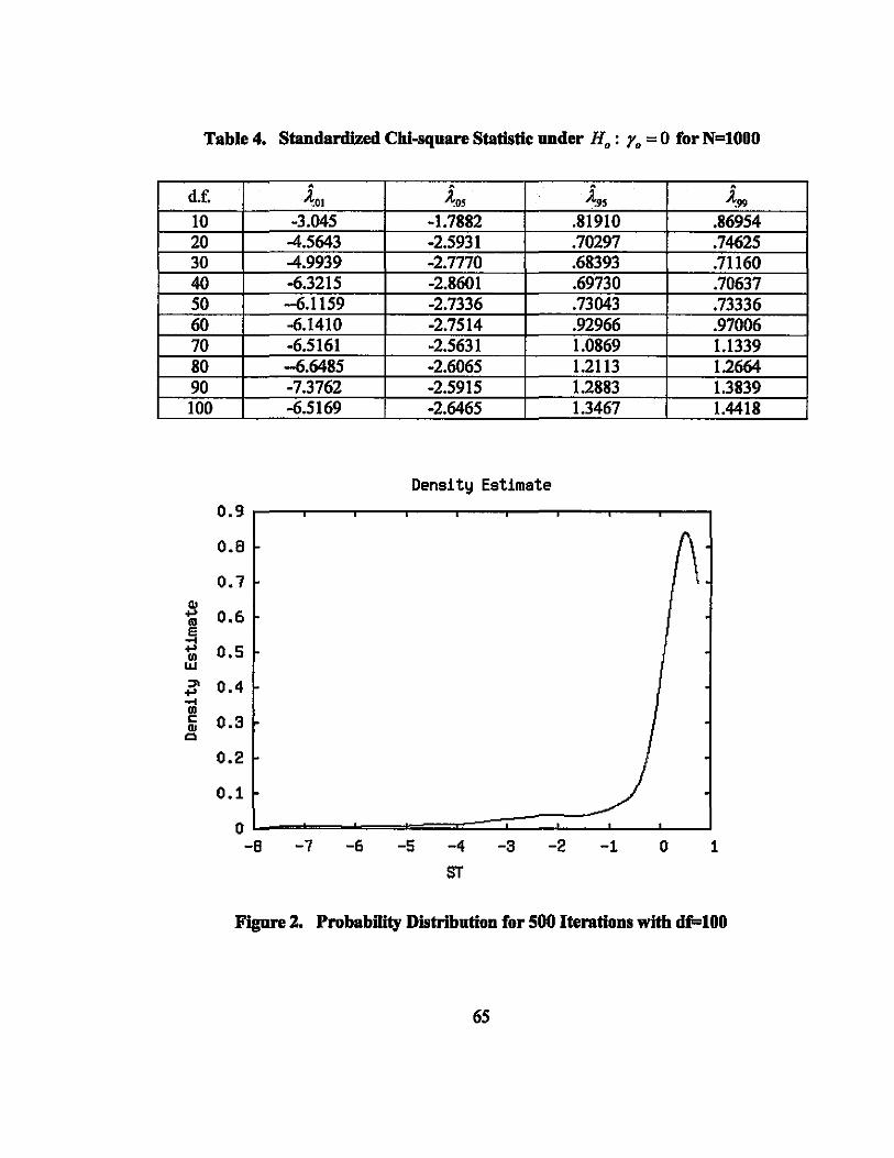
Table 4. Standardized Chi-square Statistic under Ho: Yo = 0 for N=lOOO

• • . • • d.f. .lOI .los .l95 A:!>9 10 -3.045 -1.7882 .81910 .86954 20 -4.5643 -2.5931 .70297 .74625 30 -4.9939 -2.7770 .68393 .71160 40 -6.3215 -2.8601 .69730 .70637 50 -6.1159 -2.7336 .73043 .73336 60 -6.1410 -2.7514 .92966 .97006 70 -6.5161 -2.5631 1.0869 1.1339 80 -6.6485 -2.6065 1.2113 1.2664 90 -7.3762 -2.5915 1.2883 1.3839 100 -6.5169 -2.6465 1.3467 1.4418

Density Estimate 0.9

0.8 " 0.7 \ CII +' 0.6 lIJ e .... +' 0.5 CD UJ

~ 0.4 +' .... CD c: 0.3 01

Q

0.2

0.1

0 .. -8 -7 -6 -5 -4 -3 -2 -1 0 1

ST

Figure 2. Probability Distribution for 500 Iterations with cJtl=lOO

65

Densi ty Estimate

0.6

0.5

CIJ .... 0.4 OJ e ..... .... '" UJ 0.3 ::>\ .... ..... '" c: 0.2 CIJ

0

0.1

0 -12 -10 -8 -6 -4 -2 o 2

ST

Figure 3. Probability Distribution for 1000 Iterations with df.=IOO

As the sample size increases, ..i -+ A. in probability distribution. Therefore, the

standardized Chi-squares distribution in Table 5 can be used for testing Ho: Yo = 0 as an

approximation for large sample cases. The advantage of using the standardized Chi-

squares are in two-fold: (1) it converges to the standard normal distribution though the

convergence is very slow as the sample size increases (as can be seen in Table 5); (2) its

values are finite instead of increasing as the degrees of freedom increase.

66

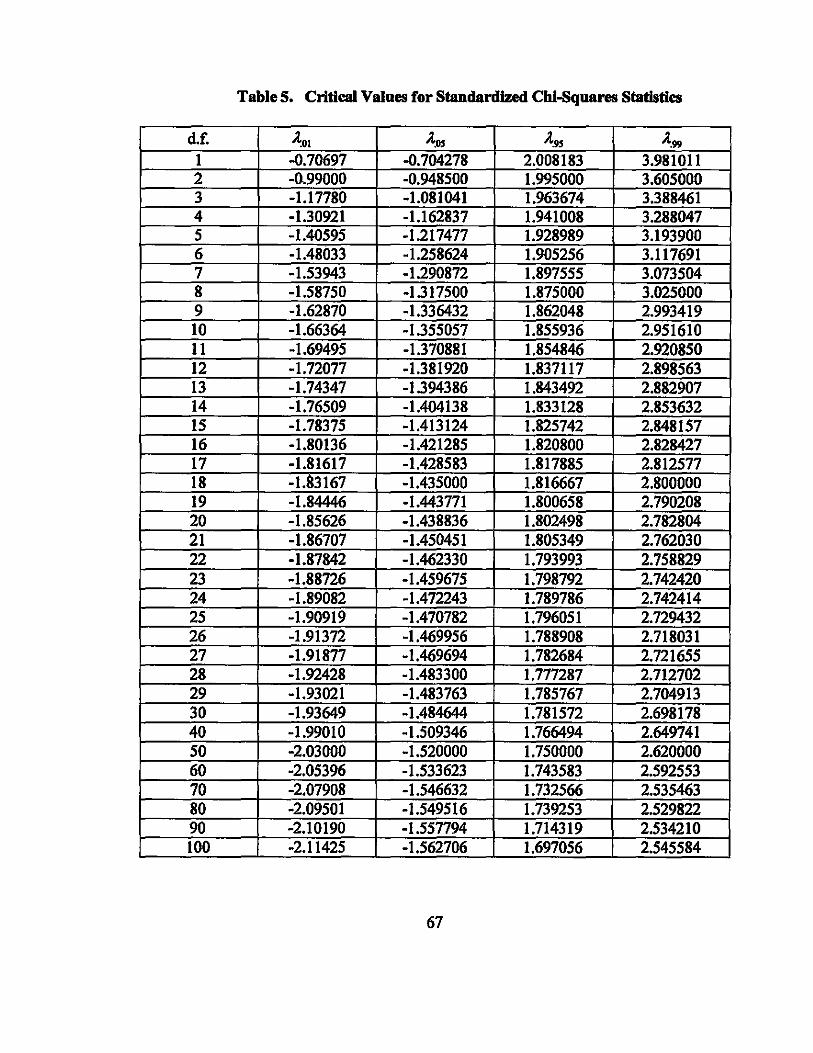
Table 5. Critieal Values for Standardized Chi-Squares Statisties

d.£ A:OI .4os .4.9, .4.99

1 -0.70.697 -0.704278 2.0.0.8183 3.9810.11 2 -0..990.0.0. -0.94850.0 1.995000 3.60.50.00. 3 -1.17780 -1.0.81041 1.963674 3.388461 4 -1.30.921 -1.162837 1.9410.08 3.288047 5 -1.40595 -1.217477 1.928989 3.19390.0. 6 -1.480.33 -1.258624 1.90.5256 3.117691 7 -1.53943 -1.290.872 1.897555 3.0.7350.4 8 -1.58750 -1.31750.0 1.87500.0. 3.0250.0.0. 9 -1.62870. -1.336432 1.862048 2.993419 10. -1.66364 -1.355057 1.855936 2.951610. 11 -1.69495 -1.370.881 1.854846 2.920850. 12 -1.720.77 -1.381920 1.837117 2.898563 13 -1.74347 -1.394386 1.843492 2.88290.7 14 -1.7650.9 -1.404138 1.833128 2.853632 15 -1.78375 -1.413124 1.825742 2.848157 16 -1.80.136 -1.421285 1.820.80.0. 2.828427 17 -1.81617 -1.428583 1.817885 2.812577 18 -1.83167 -1.43500.0. 1.816667 2.800.0.00. 19 -1.84446 -1.443771 1.80.0658 2.79020.8 20. -1.85626 -1.438836 1.80.2498 2.782804 21 -1.8670.7 -1.450451 1.80.5349 2.762030. 22 -1.87842 -1.462330. 1.793993 2.758829 23 -1.88726 -1.459675 1.798792 2.742420. 24 -1.890.82 -1.472243 1.789786 2.742414 25 -1.90.919 -1.470782 1.796051 2.729432 26 -1.91372 -1.469956 1.788908 2.7180.31 27 -1.91877 -1.469694 1.782684 2.721655 28 -1.92428 -1.483300. 1.777287 2.71270.2 29 -1.930.21 -1.483763 1.785767 2.704913 30 -1.93649 -1.484644 1.781572 2.698178 40. -1.990.10. -1.50.9346 1.766494 2.649741 50. -2.0.30.0.0. -1.520.0.0.0. 1.750.0.0.0 2.620.0.0.0. 60. -2.05396 -1.533623 1.743583 2.592553 70 -2.07908 -1.546632 1.732566 2.535463 80 -2.0.9501 -1.549516 1.739253 2.529822 90 -2.10190 -1.557794 1.714319 2.534210. 100 -2.11425 -1.56270.6 1.697056 2.545584

67

2.7. Conclusion

This essay added some theoretical rigor to the exiting analysis of the adaptive

regression model. and introduced a new approach for testing the statistical significance of

the instability parameter. The test statistic herein introduced is a new approach in the

sense that it is not directly based on ML estimator of the instability parameter. Rather, it

is a residual based statistic to avoid the problems associated with the direct approach. As

theoretically expected, the test statistic tends towards the standardized Chi-square as the

sample size and iteration number increase. A refined table for critical values may be a

useful reference for the significance test in small sample cases. If the sample size is

sufficiently large, the standardized Chi-square table shown in this essay can be used.

68

AppendixB

The first-order condition for lI18.Yimizjng L(y) is

(BI)

Notetbat

I -2tr( KIA,A-IArA-lse')tr( A-1se')+[ tr(A -lArA -lse')1 L71 = 2 [tr(A- lse')1

(B2)

Substitute Equation (BI) into Equation (B2).

69

= (B3)

= _T[.!.t( d,-l It d,-l )2]<0 2 T/ol (d,-l)r+l T,al(d,-l)r+l .

(B4)

70

AppendixC

If r. = 0 is false,

T ~ -2 £,..p,

m(O) = '~1 TIT -2 -L p,

T '~1 (d,-I)g+1

sotbat

T

,

pJimrp(O) = L[(d,-I)r. +IJ '~1

T T(T 1) =r.L(d,-I)+T= - r.+T > T.

M 2

If r. = 1 is false, then

T _2

L P,

(1) M d, rp = I T -2 ' -L p,

T M (d,-I)g+1

sotbat

71

(el)

plimtp(I)= t (d,-I)y. +1 ,.1 d,

T T

= y.L (1-d,-I)+ Ld,-I =-Ty. +2T =T(2-y.) ~ T. (C2) let 1 ... 1

T

note that L d,-I = 2T as shown in Appendix D. '·1

72

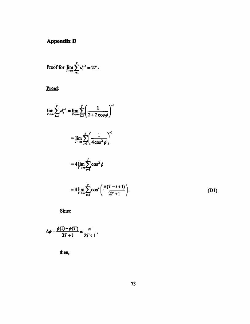
AppendixD

T

Prooffor lim Ld;1 = 2T. T-t<ID 1 ... 1

Proof:

lim d-I - lim 1 T T ( )-1 T __ ~ , - T __ ~ 2+200891

= 4 lim toos2(Il(T-t+l)). r_,al 2T+l

Since

!J.¢- ¢(I)-¢(T) 2T+l

then,

Il 2T+l'

(Dl)

73

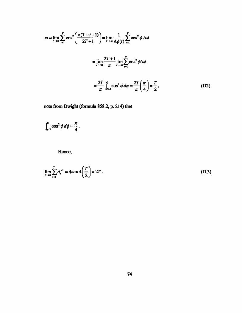
W slim ±COS2 (g(T -1+ 1)) = 1im_1_±cos2 ¢ l\¢ T ...... • =1 2T + 1 T __ l\¢(/) .=1

(D2)

note from Dwight (formula 858.2, p. 214) that

Hence,

lim ±d,-I =4W=4(T) =2T. r_.=1 2

(D.3)

74

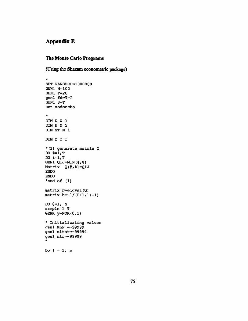
AppendixE

The Monte Carlo Programs

(Using the Sbazam econometric package)

* SET RANSEED=lOOOOOO GENl N=lOO GENl T=20 gen1 fd=T-l GEN1 S=T set nodoecho

* DIM U N 1 DIM W N 1 DIM ST N 1

DIM Q T T

*(1) generate matrix Q 00 1I=l,T 00 %=l,T GEN1 QIJ=MINCi,%) Matrix QCi,%)=QIJ ENOO ENOO *end of (1)

matrix D=eigvalCQ) matrix h=-1/CDC1,l)-1)

DO $=1, N sample 1 T GENR y=NORCO,l)

* Initializating values gen1 MLF =-99999 gen1 mltst=-99999 gen1 mlr=-99999 *

Do ! = 1, s

75

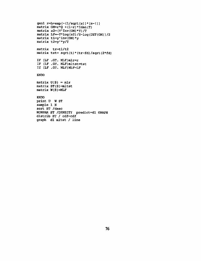
genl r=h+exp(-(l/sqrt(s»*(s-!» matrix OM=r*Q +(l-r)*Iden(T) matrix s2=(Y'Inv(OM)*Y)/T matrix LF=-T*log(s2)/2-log(DET(OM»/2 matrix tl=y'inv(OM)*y matrix t2=y'*y/T

matrix tr=tl/t2 matrix tst= sqrt(t)*(tr-fd)/sqrt(2*fd)

IF (LF .GT. MLF)mlr=r IF (LF .GT. MLF)mltst=tst If (LF • GT. MLF) MLF=LF

ENDO

matrix U($) = mlr matrix ST($)=mltst matrix W($)=MLF

ENDO print U W ST sample 1 N sort ST /desc NONPAR ST /DENSITY predict=dl GRAPH distrib ST / cdf=cdf graph dl mltst / line

76

References

Box, G., G. Jenkins (1970) TIME SERIES ANALYSIS: FORECASTING AND CONTROL, San Francisco: Holden-Day.

Cooley, T. F. (1971) "Estimation in the Presence of Sequential Parameter Variation," Ph.D. Thesis, University of Pennsylvania.

Cooley, T.F., E.C. Prescott (1973a) "Adaptive Regression Model," International Economics Review, 14,364-71.

Cooley, T.F., E.C. Prescott (1973b) "Test of an Adaptive Regression Model," Review of Economics and Statistics, 55, 248-56.

Cooley, T. F., E.C. Prescott (1973c) "Systematic (Nonrandom) Variation Models Varying Parameter Regression: a Theory and Some Applications," Annals of Economic and Social Measurement, 2, 463-73.

Cooley, T. F., E. C. Prescott (1976) "Estimation in the Presence of Stochastic Parameter Variation," Econometrica, 44, 167-75.

Cooley, T. F., S. J. DeCarno (1977) "Rational Expectations in American Agriculture, . 1867-1914," Review of Economics andStatistics, 59, 9-17.

Davidson, R., J.G. MacKinnon (1993) EsTIMATION AND INFERENCE IN EcONOMETRICS, Oxford University Press, New York.

Dickey, D.A., W. A. Fuller (1979) "Distribution of the Estimators for Autoregressive Time Series with a Unit Root," Journal of American Statistical Association, 74, 427-31.

Dickey, D.A., W. A. Fuller (1981) "Likelihood Ratio Statistics for Autoregressive Time Series with a Unit Root," Econometrica, 49, 1057-72.

Dwight, H.B. (1961) TABLES OF INTEGRALS AND OTHER MATHEMATICAL DATA, Macmillan, New York.

77

Engle, R.F., C. W J. Granger (1987) "Cointegration and Error Correction; Representation Estimation and Testing," Econometrica, 55 (2), 251-76.

Entorf, H. (1997) "Random Walks with Drifts: Nonsense Regression and Spurious Fixed­Effect Estimation," Journal o/Econometrics, 80, 287-96.

Fuller, W. (1976) INTRODUCTIoN TO STATISTICAL TiME SERIES. New York: John Wiley.

Granger, C., P. Newbold (1974) "Spurious Regression in Econometrics," Journal 0/ Econometrics, 2, 111-20.

Granger, C.W.J., N., Swanson (1997) "An Introduction to Stochastic Unit-root Processes," Journal o/Econometrics, 80, 35-62.

Guilkey, D. K., P. Schmidt (1989) "Extended Tabulations for Dickey-Fuller Tests," Econometrics Letters, 31, 355-7.

Haldrup, N. (1994) "The Asymptotics of Single -equation Cointegration regressions with 1(1) and 1(2) Variables," Journal o/Econometrics, 63,153-81.

Hall, R. E. (1978) "Stochastic Implications of Life Cycle-Permanent Income Hypothesis: Theory and Evidence," The Journal 0/ Political Economy, 86 (6), 971-87.

Hamilton, J.D. (2000) "A Parametric Approach to Flexible Nonlinear Inference," Econometrica, 69, 801-12.

Han, K. T. (1997) "Three Essays in Econometrics: Idempotent Matrix, Adaptive Regression, and Unit Root Test," Ph.D. Thesis, University of Hawai'i at Manoa.

Hansen, L. P., K. J. Singleton (1983) "Stochastic Consumption, Risk Aversion, and Temporal Behavior of Asset Returns," The Journal 0/ Political Economy, 91(2), 249-65.

Hoel, P.G., Port, S.C., CJ. Stone (1971) INTRODUCTION TO PROBABILITY THEORY, Houghton Miftlin, Boston.

1m, E. (1990) "Limit Variance ofg: Problem," Econometric Theory, Vol. 6,486-87.

1m, E. (1992) "Limit Variance of g: Solution," Econometric Theory, Vol. 8,250-53.

Kennedy, P. A. (1992) GUIDE TO EcONOMETRICS (3R1 cd.), the MIT Press.

78

Lee, T.H., White, H., C.W J., Granger (1993) "Testing for Neglected Nonlinearity in Time Series Models," Journal o/Econometrics, 56, 269-90.

Lee, Y.S., Kim, T.H., P. Newbold (2005) "Spurious Nonlinear Regressions in Econometrics," Economics Letters, 87(3), 301-06.

Leung, S.F., S. Yu (2001) "The Sensitivity of the RESET Tests to Disturbance Autocorrelation in Regression Analysis," Empirical Economics, 26, 721-26.

Mankiw, N. G. (1982) "Hall's Consumption Hypothesis and Durable Goods," Journal 0/ Monetary Economics, 10, 417-25.

Mankiw, N. G. (1985) "Consumer Durables and the Real Interest Rate," The Review 0/ Economics and Statistics, 67(3), 353-62.

Marmol, F. (1998) "Spurious Regression Theory with Nonstationary Fractionally Integrated Processes," Journal o/Econometrics, 84, 233-50.

Park, J.Y., P.C.B. Phillips (2001) "Nonlinear Regressions with Integrated Time Series," Econometrica,69,117-61.

Pindyck, R. S., D.L. Rubinfeld (1998) EcONOMETRIC MODELS AND EcONOMIC FORECASTS (4th ed.).

Phillips, P .C.B. (1986) "Understanding Spurious regressions in Econometrics," Journal 0/ Econometrics, 33, 311-40.

Phillips, P.C.B. (1987) "Time Series Regression with a Unit Root," Econometrica, 55, 277-301.

Phillips, P .C.B., S.N. Durlauf (1986) "Multiple Time Series Regressions with Integrated Processes," Review o/Economic Studies, 53, 473-95.

Porter, R.D., A.K. Kashyap (1984) "Autocorrelation and the Sensitivity of RESET," Economics Letters, 14,229-33.

Romer, D. (2001) ADVANCED MACROECONOMIcs, McGraw-Hill Higher Education, Boston.

Schmidt, P. (1990) "Dickey-Fuller Tests with Drifts," in ADVANCES IN EcONOMETRICS Vol. 8. (Fomby, T. B., G. F. Rhodes, eds.), Greenwich, CT: JAI Press.

79

Essay Three

Nested AR (1) Disturbance Model

3.1. Introduction

Nested model has been gaining popularity in econometric studies. Greene (2006)

gives an introduction of the nested models. In econometrics, a model can be written as a

special case of another mode. In this case, the two models are nested, in which some

restrictions are imposed on the parameters of one model.

In nested AR(1) disturbance model, there are two types of simple specifications of

the residual term, one is the first-order autocorrelation and the other the adaptive

regression model. This essay synthesizes these two types of residual specifications,

which may better represent the actual reaIization of the residual.

The adaptive regression model is a model where only intercept is subject to

transitory and permanent changes,

y, =a, +x,P, (1)

where

80

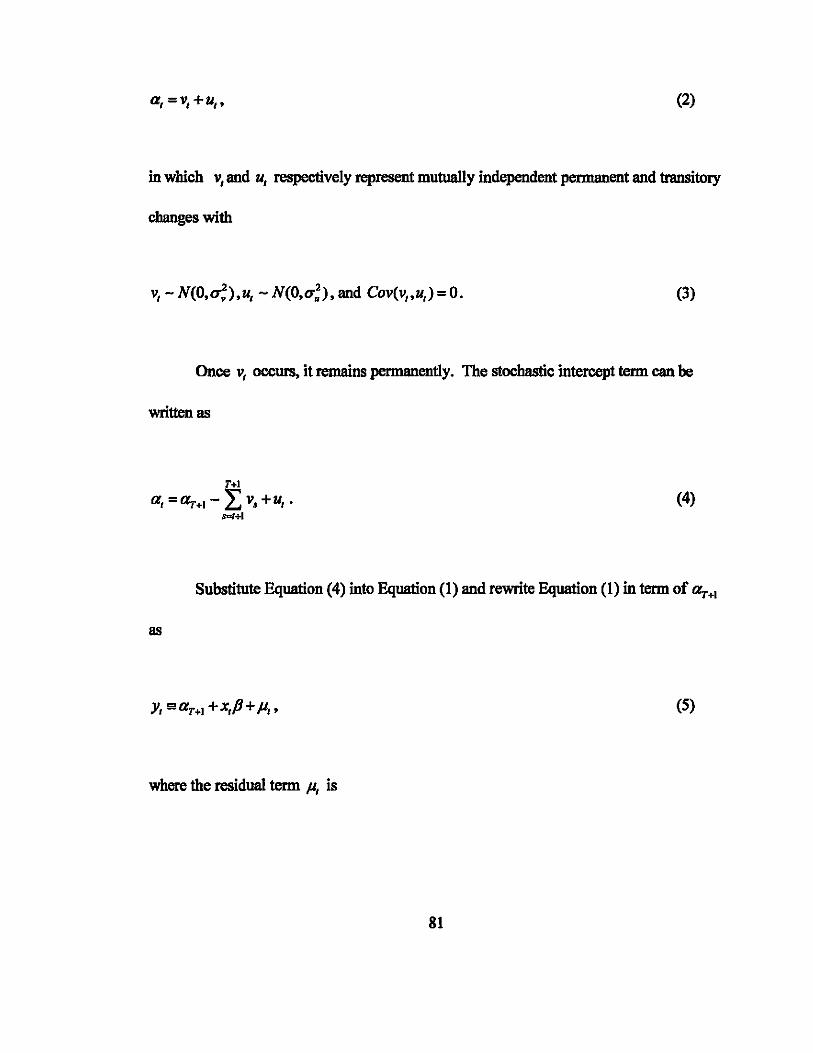
a, =v,+u" (2)

in which v, and u, respectively represent mutually independent permanent and transitory

changes with

v, -N(O,u;),u, -N(O,O";), and Cov(v"u,) =0. (3)

Once v, occurs, it remains permanently. The stochastic intercept term can be

written as

T+1

a, =aT+1 - L v, +u,. "",,+1

(4)

Substitute Equation (4) into Equation (1) and rewrite Equation (1) in term of aT+1

as

y, a aT+1 + x,fJ + /I" (5)

where the residual term /I, is

81

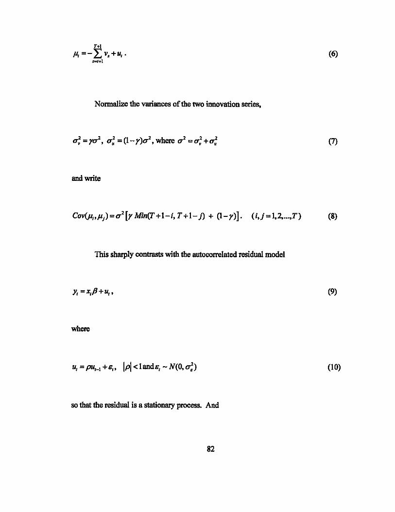
T+I

JI, =-LV. +U,. s,,",+1

Normalize the variances of the two innovation series,

and write

(6)

(7)

Cov{J.l"JlJ)=u2 [r Min(T+l-/, T+l- j) + (l-r)]. (i,j = l,2, ...• T) (8)

This sharply contrasts with the autocorrelated residual model

y, =x,P+u" (9)

where

(10)

so that the residual is a stationary process. And

82

E[u,]=O forallt.

0'2 Var[u,]=~.

I-p (11)

Cov[u,.u.]

This essay is organized as follows. Section 3.2 is the literature review. Section

3.3 introduces nested autocorrelation. Section 3.4 diagonalizes O(Y.p). Section 3.5

develops the maximwn likelihood estimation. Section 3.6 discusses the information

matrix and the Cramer-Rao Lower Bounds. Section 3.7 is the simulation analysis.

Section 3.8 concludes.

3.2. Literature Review

An autoregressive process of order p can be written as

83

(12)

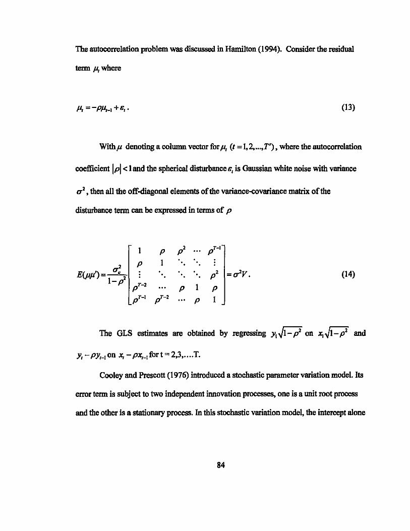
The autocorrelation problem was discussed in Hamilton (1994). Consider the residual

term lit where

(13)

Withp denoting a column vector for P, (t = 1.2, ...• T'). where the autocorrelation

coefficient Ipi < 1 and the spherical disturbance H, is Gaussian white noise with variance

0'2. then all the off-diagonal elements of the variance-covariance matrix of the

disturbance term can be expressed in terms of p

1 P p2 pT-1

P 1 . . 2

E(pp') = 1 0'. 2 . . p2 - 2V (14) . . . . . -0' •

-p pT-2 1 p P pT-1 pT-2 ... P 1

The GLS estimates are obtained by regressing YI ~1- p2 on -Xi ~1- p2 and

Y, - PYt-I on x, - pXt-I for t = 2.3 •.... T.

Cooley and Prescott (1976) introduced a stochastic parameter variation model. Its

error term is subject to two independent innovation processes. one is a unit root process

and the other is a stationary process. In this stochastic variation model. the intercept alone

84

is subject to permanent and transitory variations. It is referred to as the adaptive

regression model in Cooley and Prescott (1973a, 1973b, 1976).

McCabe et aI. (2003) discussed the persistence element of the autoregression

process. A persistent series contains a permanent component, in which the impact of a

shock will continue indefinitely. A transitory series contains only a transitory component,

in which the impact of a shock will dissipate over time.

There are three kinds of standard measures for persistence. First, the long-run

impulse response function measures the impact of a shock on the level of a time series.

Second, the long-run variance ratio function measures how much the permanent

component in the series will cause to the variation in the first differenced time series.

Third, the long-run autocorrelation function measures the correlation between two

periods of the time series that are infinitely far apart. An integrated I( d) model is

nonpersistent if d is less than unity and persistent if it is equal to one. Brockwell and

Davis (1991) and Baillie (1996) suggested that a decay in both the impulse response and

autocorrelation functions indicate a lack of persistence for stationary fractional models,

where d < 0.5.

Cramer (1961) provided a useful decomposition of both stationary or

nonstationary time series, which is a generalization of the decomposition of Wold (1938)

for stationary time series. In his approach, a nondeterministic series is described in terms

of a linear process, where the coefficients are uncorrelated with zero mean and possibly

different variance, but may depend on time and the disturbances. 1jsstheim (1976)

85

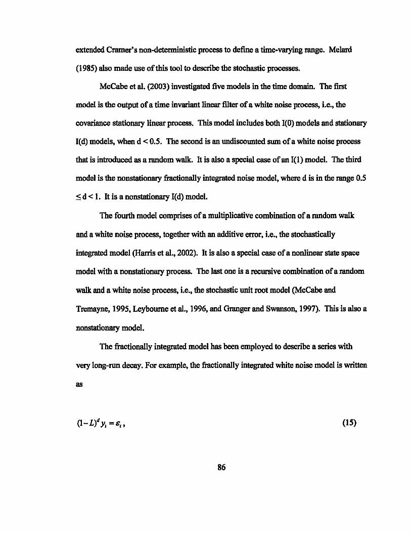
extended Cramer's non-deterministic process to define a time-varying range. Melard

(1985) also made use of this tool to describe the stochastic processes.

McCabe et aI. (2003) investigated five models in the time domain. The first

model is the output of a time invariant linear filter of a white noise process, i.e., the

covariance stationary linear process. This model includes both I(O} models and stationary

I(d} models, when d < 0.5. The second is an undiscounted sum of a white noise process

that is introduced as a random walk. It is also a special case of an I(I} model. The third

model is the nonstationary fractiona1ly integrated noise model, where d is in the range 0.5

~ d < 1. It is a nonstationary I( d} model.

The fourth model comprises of a multiplicative combination of a random walk

and a white noise process, together with an additive error, i.e., the stochastically

integrated model (Harris et aI., 2002). It is also a special case of a nonlinear state space

model with a nonstationary process. The last one is a recursive combination of a random

walk and a white noise process, i.e., the stochastic unit root model (McCabe and

Tremayne, 1995, Leybourne et aI., 1996, and Granger and Swanson, 1997). This is also a

nonstationary model.

The fractionally integrated model has been employed to describe a series with

very long-run decay. For example, the fractionally integrated white noise model is written

as

(I-Lty, =&" (IS)

86

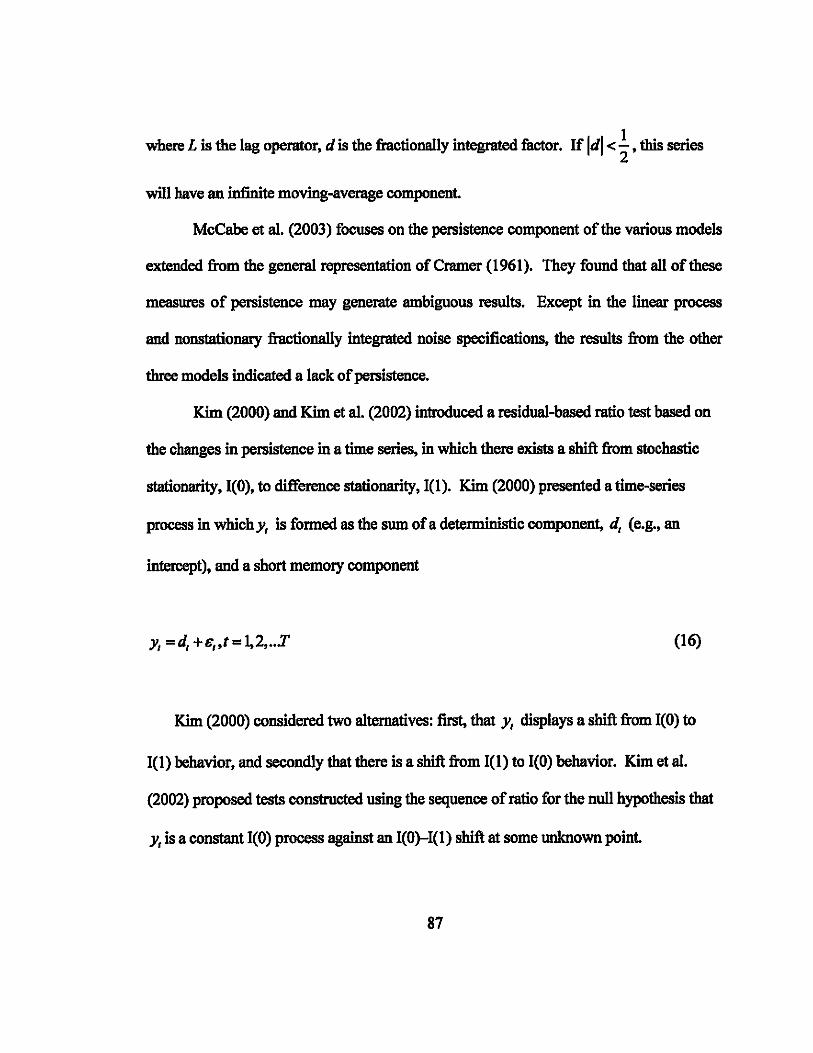
where L is the lag operator, d is the fractionally integrated factor. If Idl < 1., this series 2

will have an infinite moving-average component.

McCabe et aI. (2003) focuses on the persistence component of the various models

extended from the general representation of Cramer (1961). They found that all of these

measures of persistence may generate ambiguous results. Except in the linear process

and nonstationary fractionally integrated noise specifications, the results from the other

three models indicated a lack of persistence.

Kim (2000) and Kim et aI. (2002) introduced a residual-based ratio test based on

the changes in persistence in a time series, in which there exists a shift from stochastic

stationarity, 1(0), to difference stationarity, 1(1). Kim (2000) presented a time-series

process in whichy, is formed as the sum of a deterministic component, d, (e.g., an

intercept), and a short memory component

y, = d, +&"t = 1,2, .. .7' (16)

Kim (2000) considered two alternatives: first, that y, displays a shift from 1(0) to

1(1) behavior, and secondly that there is a shift from 1(1) to 1(0) behavior. Kim et aI.

(2002) proposed tests constructed using the sequence of ratio for the null hypothesis that

y, is a constant 1(0) process against an I(O}-l(I) shift at some unknown point.

87

Leybournea and Taylor (2004) extended Kim et al. (2002)'8 methodology of the

residual-based ratio tests using a non-parametric approach. They used Monte Carlo

simulation to compare the power properties of the non-parametrically modified ratio­

based tests and the corresponding unmodified tests for a finite-sample size. They

investigated ARMA(I, 1) process in a time series.

The ARMA(I, I) process can be derived from many dynamic optimi7}!tion

framework. For example, the first order condition for a consumption model with the

stock of consumer durables, Kb can be written as an Euler equation

(17)

Assuming an additive error term, we then obtain:

(18)

After several algebraic manipulations, we obtain the optimal capital stock of

durable goods as

(19)

88

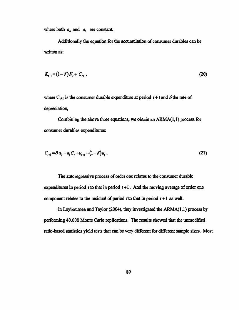
where both a. and a l are constant

Additionally the equation for the accumulation of consumer durables can be

written as:

where Ct.. is the consumer durable expenditure at period 1+ 1 and 8the rate of

depreciation,

(20)

Combining the above three equations, we obtain an ARMA(I,I) process for

consumer durables expenditures:

C"I =8 Do +"tC, +u'+I-(1-8)u, .. (21)

The autoregressive process of order one relates to the consumer durable

expenditures in period Ito that in period I + I. And the moving average of order one

component relates to the residual of period I to that in period I + 1 as well.

In Leybournea and Taylor (2004), they investigated the ARMA(I,I) process by

performing 40,000 Monte Carlo replications. The results showed that the unmodified

ratio-based statisties yield tests that can be very different for different sample sizes. Most

89

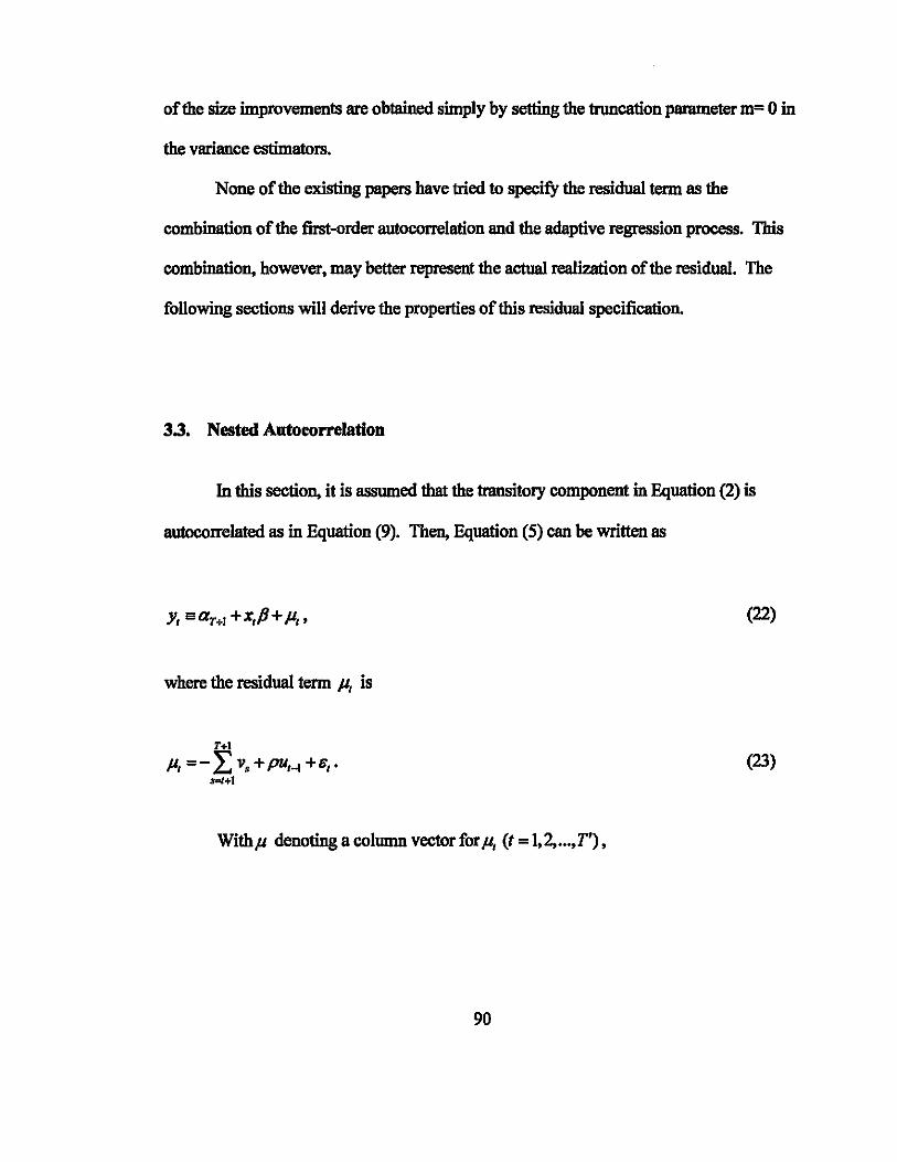
of the size improvements are obtained simply by setting the truncation parameter m= 0 in

the variance estimators.

None of the existing papers have tried to specify the residual term as the

combination of the first-order autocorrelation and the adaptive regression process. This

combination. however. may better represent the actuaI realization of the residual. The

following sections will derive the properties of this residual specification.

3.3. Nested Autocorrelation

In this section. it is assumed that the transitory component in Equation (2) is

autocorrelated as in Equation (9). Then, Equation (5) can be written as

where the residual term #, is

T+1

#, =-L V.+PUH +&,. ....,+1

With # denoting a column vector for #, (1 = 1.2, .... T') •

90

(22)

(23)

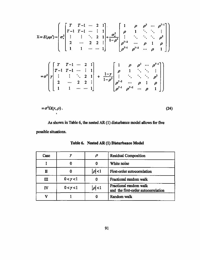
T T-l 2 1 1 P p2 pT-t

T-l T-l 1 p 1 2

r. a E(pp') = U2 . 2 1 U. . . p2 . +--• I_p2 2 2 2 pT-2 P 1 p 1 1 1 pT-t pT-2 p 1

T T-I 2 1 1 P p2 pT-t

T-I T-I 1 1 . . p .

=u2 . . 2 1 I-r . p2 r + l_p2 . .

2 2 2 pT-2 P I p 1 I I pT-t pT-2 p 1

au2n(y,p) . (24)

As shown in Table 6, the nested AR (1) disturbance model allows for five

possible situations.

Table 6. Nested AR (1) Disturbanee Model

Case r p Residual Composition

I 0 0 Whitenolse

n 0 Ipl<1 First-order autocorrelation

m O<r<1 0 Fractioual random walk

IV O<r<1 Ipl<1 Fractional random walk and the first-order autocorrelation

V 1 0 Random walk

91

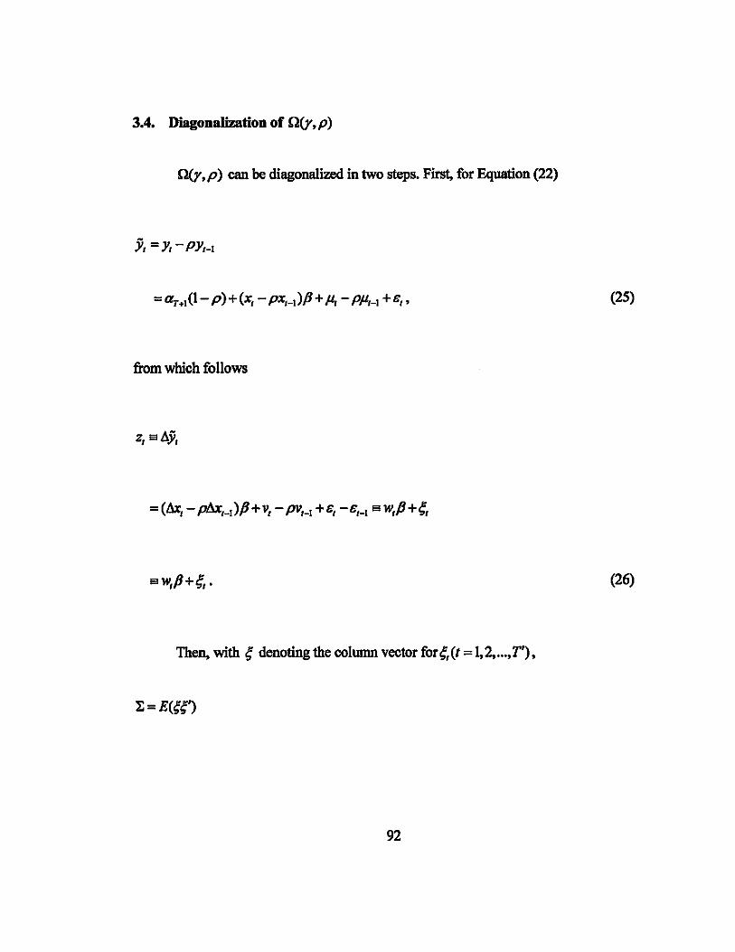
3.4. Diagonalization of Q(y.p)

Q(y.p) can be diagonaIized in two steps. First, for Equation (22)

Yt = Yt - PYt-1

(25)

from which follows

Zt 5l AYt

(26)

Then. with q denoting the colwnn vector for" (t = 1.2. .•.• T') •

92

I+p' -p 0 0 2 -I 0 ... 0

-p I+p' -I 2 . =0'2 r 0 . 0 +(1-r) 0 0 . . I+P' -p 2 -I

0 0 -p I+p' 0 ... 0 -I 2

yp2 -r+2 -rp+r- i 0 0

-rp+r- i rp2-r+2 . · . . =0-

2 0 . . · .

0 . . . . . · rp2-r+2 -rp+r- i 0 0 -rp+r-I rp2-r+2

(27)

Write Equation (26) in matrices.

z=WP+~. (28)

There exists C such that CC' = C'C = IT' and C'QC = A where A denotes the

diagonal matrix consisting of eigenvalues of r(y. p). The eigenvalues for the type of

matrix as r(y,p) can be analytically expressed as (Bellman, 1960. p. 215)

,t(t) = rp2 -r-2+2(yp-r+ I)COS(j6t). (t = 1. 2, .... T' ) (29)

93

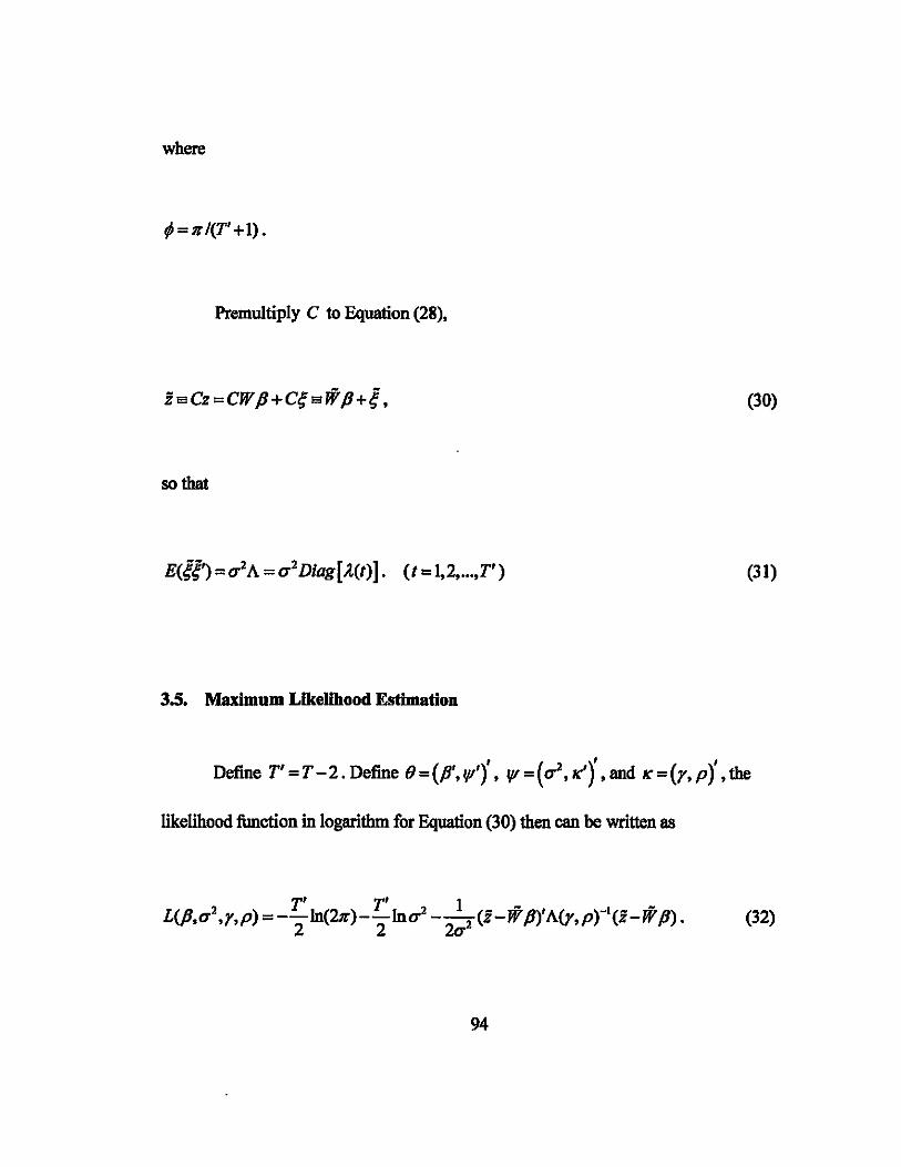
where

;=nl(T'+I).

Premultiply C to Equation (28),

(30)

sotbat

-- 2 2 [ ] , E(~f) = 0' A = 0' Diag l(t). (t = 1,2, ... ,T ) (31)

3.5. Maximum Likelihood Estimation

Define T' = T -2. Define (J = (P', /fI')' , /fI =(0'2, K')' ,and K =(r, p)' , the

likelihood function in logarithm for Equation (30) then can be written as

94

The first and second derivatives of Equation (32) are as follows

(33.1)

L olnL T 1 (- W-P)'A-1(- W-P) 8---=---+--Z- Z- • .., 00'2 20'2 20'4 (33.2)

(33.3)

(33.4)

(33.5)

(33.6)

(33.7)

95

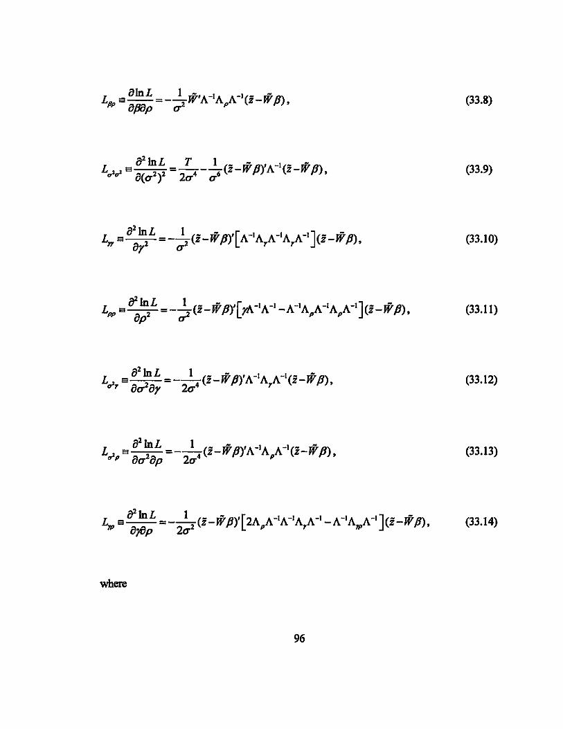
(33.8)

(33.9)

(33.10)

(33.11)

(33.12)

(33.13)

(33.14)

where

96

A = Diag[l(t)] = Diag[yp2 - y+2+2(2yp-y+ I)COS(¢t)]. (33.15)

Ap = Diag[ l(t)p] = 2yDiag[p+COS(¢t)]E32yDiag[ 1(t)]. (33.16)

Ar = Diag[ l(t)r] = Diag[p2 -1 + 2(p-l)COS(¢t) ]. (33.17)

APr = Ayp = Diag[ l(t)yp] = Diag[2p+2COS(¢t)]. (33.18)

From Equations (33.1) and (33.2).

2 1 (- Wb-)'A-1(- Wb-) s =- z- z-. T

(34)

Substitute b and S2 into Equation (21). the likelihood function concentrated

inV'becomes:

97

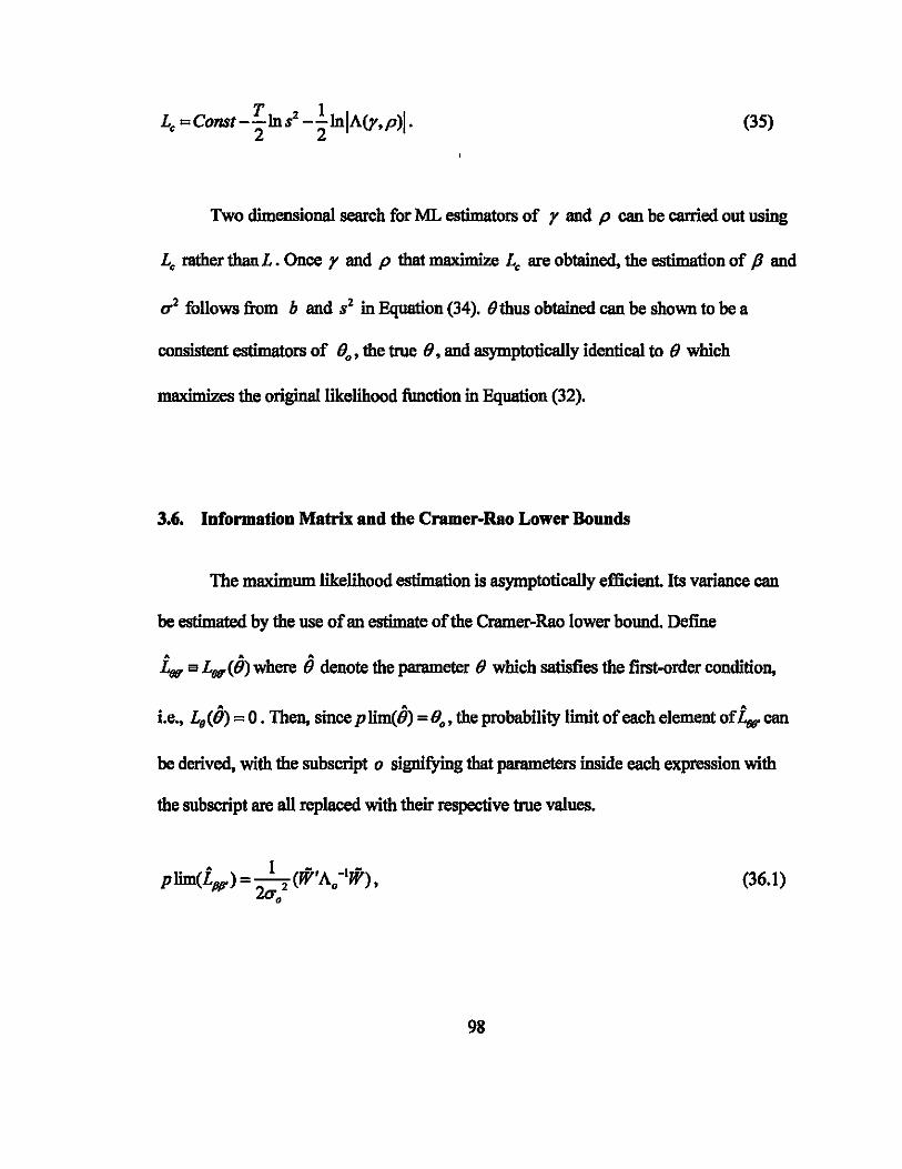
(35)

Two dimensional search for ML estimators of r and p can be carried out using

Lc rather thanL. Once r and p that maximize Lc are obtained, the estimation of p and

0-2 follows from b and 82 in Equation (34). Othus obtained can be shown to be a

consistent estimators of 0., the true 0, and asymptotically identical to 0 which

maximizes the original likelihood function in Equation (32).

3.6. Information Matrix and the Cramer-Rao Lower Bounds

The maximum likelihood estimation is asymptotically efficient. Its variance can

be estimated by the use of an estimate of the Cramer-Rao lower bound. Define

LQII a LQII (0) where 0 denote the parameter 0 which satisfies the first-order condition,

i.e., Lo(O) = O. Then, since plim(O) =0., the probability limit of each element ofLQII can

be derived, with the subscript 0 signifying that parameters inside each expression with

the subscript are all replaced with their respective true values.

lim(L )=_l_(W'A -·W) p 'fJfJ' 20"2 • , •

(36.1)

98

(36.2)

• A T' plim(L .... )=--2 4'

O'. (36.3)

plim(i, )=-~Tr(A-IA7).' er7 20' •

(36.4)

plim(i .. p )=-~ 2 Tr(A-1Ap ).,

• (36.5)

(36.6)

(36.7)

(36.8)

Based on the information matrix, the Cramer-Rao lower bounds for the variances

of r and p can be found from

Cov(D) =[ COVcft~ COV(P,,p)] Cov(,p,P} Cov(,p)

99

(37)

From Equation (37) readily follows:

(38)

Use the formula for partitioned matrix (Greene, 1997, p.33),

100

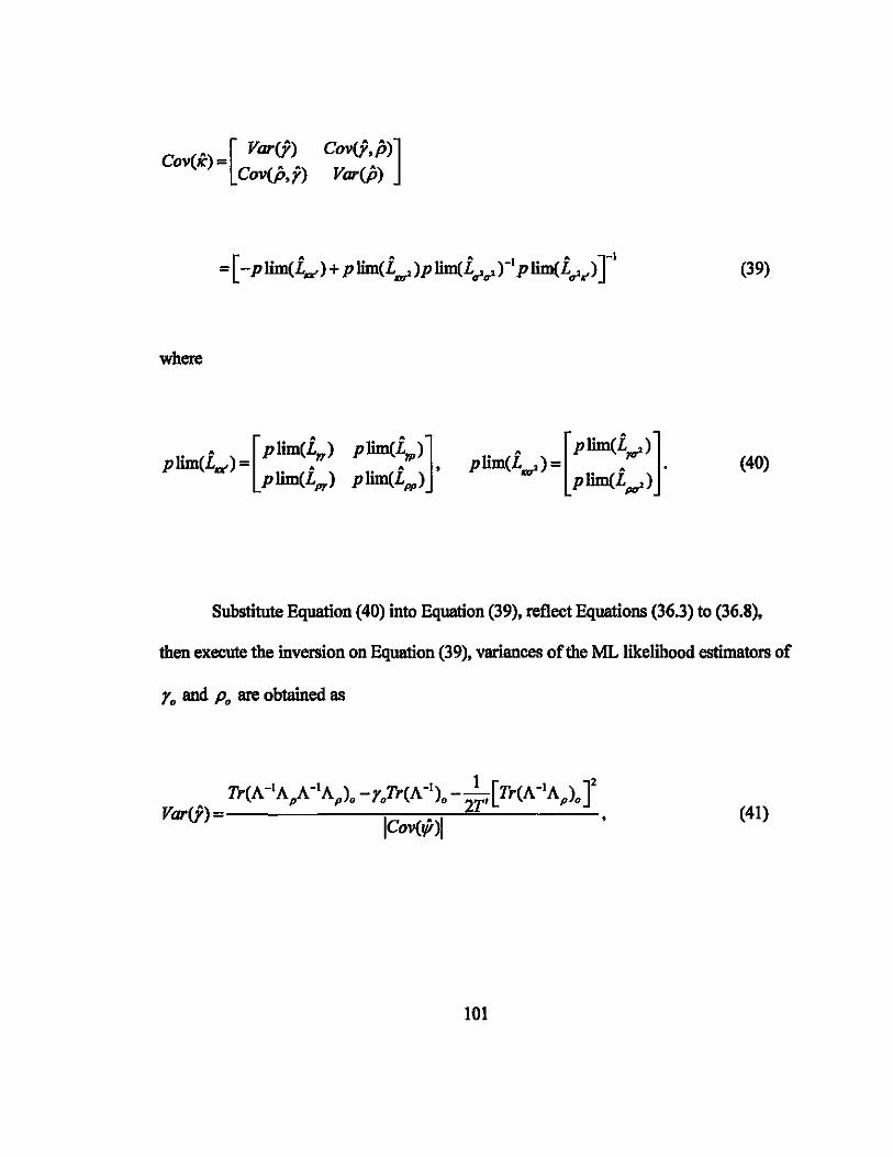
COV(K}=[ Var'!}. cov(f:P}] COV(p,r} Var(p}

(39)

where

.' [plim(ira'}] plim(L...,,) = •. p lim( L"", )

(40)

Substitute Equation (40) into Equation (39), reflect Equations (36.3) to (36.8),

then execute the inversion on Equation (39), variances of the ML likelihood estimators of

r. and p. are obtained as

VarCi) 7r(A-1ApA-1Ap ). -r.Tr(A-1

). -fr,[7r(A-1Ap}.J ICov(v;)1

101

(41)

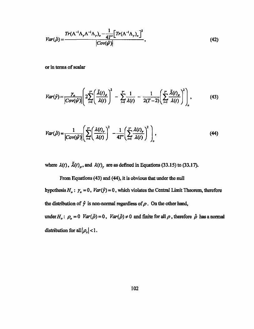
(42)

or in terms of scalar

Var(j) = Yo 2£ .iI.(t)p _ £-1- _ 1 £ .iI.(t)p [ ( - )2 ( _ )2) iCov(lfr)i /Q\ .iI.(t) /~\ .iI.(t) 2(T -2) /Q\ .iI.(t) 0 '

(43)

• 1 ( l' (.iI.(I),)2 1 (1' .iI.(t),)2 ) Var(jJ) = iCov(lfr)i fr .iI.(t) - 4T' fr .iI.(t) o'

(44)

where .iI.(t), 1(1) p' and .iI.(t), are as defined in Equations (33.15) to (33.17).

From Equations (43) and (44). it is obvious that under the null

hypothesis Ho: Yo = O. Var(j) = O. which violates the Central Limit Theorem, therefore

the distribution of r is non-normal regardless of p. On the other hand,

under Ho: Po = 0 Var(p) = O. Var(p) ¢ 0 and finite for all P. therefore p has a normal

distribution for alliPoi < 1.

102

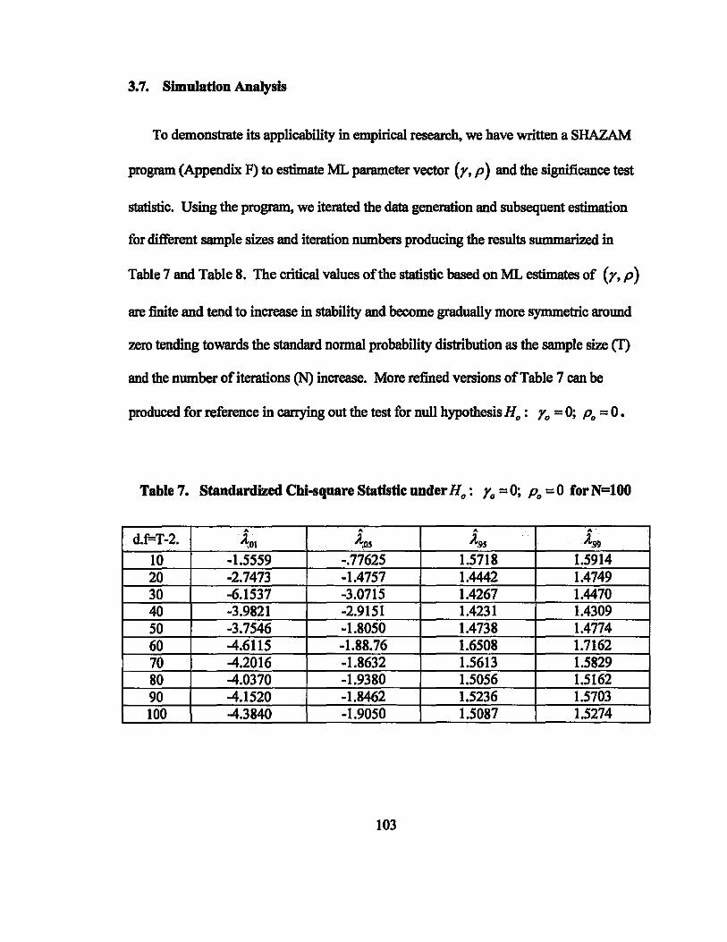
3.7. Simulation Analysis

To demonstrate its applicability in empirical research. we have written a SHAZAM

program (Appendix F) to estimate ML parameter vector (y. p) and the significance test

statistic. Using the program, we iterated the data generation and subsequent estimation

for different sample sizes and iteration numbers producing the results summarized in

Table 7 and Table 8. The critical values of the statistic based on ML estimates of (y. p)

are finite and tend to increase in stability and become gradually more symmetric around

zero tending towards the standard normal probability distribution as the sample size (T)

and the number ofiterations (N) increase. More refined versions of Table 7 can be

produced for reference in carrying out the test for null hypothesis Ho: Yo = 0; Po = 0 •

Table 7. Standardized Chi-square Statistic under Ho: Yo =0; Po =0 forN=l00

• • • • d.f-=T-2. A:ol A:o, A:95 ~

10 -1.5559 -.77625 1.5718 1.5914 20 -2.7473 -1.4757 1.4442 1.4749 30 -6.1537 -3.0715 1.4267 1.4470 40 -3.9821 -2.9151 1.4231 1.4309 50 -3.7546 -1.8050 1.4738 1.4774 60 -4.6115 -1.88.76 1.6508 1.7162 70 -4.2016 -1.8632 1.5613 1.5829 80 -4.0370 -1.9380 1.5056 1.5162 90 -4.1520 -1.8462 1.5236 1.5703 100 -4.3840 -1.9050 1.5087 1.5274

103

Table 8. Standardized Chi-square Statistic under Ho: Yo = 0; Po = 0 for N=1000

cLFT-2. A • A

199 A:OJ A:05 A..9S 10 -3.0942 -1.2583 1.5738 1.6220 20 -3.2685 -1.5273 1.5074 1.5478 30 -4.3714 -1.9532 1.4725 1.5206 40 -5.0227 -1.8645 1.4569 1.4943 50 -4.2631 -1.6520 1.4971 1.4857 60 -3.5246 -1.7024 1.6255 1.5982 70 -3.7625 -1.7534 1.5564 1.4194 80 -3.9437 -1.8068 1.5396 1.5037 90 -3.8264 -1.7603 1.5471 1.4625 100 -3.9825 -1.8214 1.5538 1.4869

3.S. Conclusion

The nested AR (1) model introduced and discussed in this essay has never been

considered e1sewhere in econometric literature. This essay provides a theoretical

framework and what appears to be a very promising statistic for testing whether adaptive

and autoregressive processes coexist in the residual term. The adaptive process herein

discussed deals with the unit root process in all possible fractions. Ignoring even a small

fraction of unit root process may lead to seriously incorrect statistical inferences as the

sample size increases.

104

AppendixF

The Monte Carlo Programs

(Using the Sba7JllD econometric package)

SET RANSEED=lOOOOOO GENl N=lOO GENl T=40 genl df=T-2 GENl C=T GENl A=T * DIM U N 1 DIM V N 1 DIM S N 1

DIM Q T T

*(1) generate matrix Q

00 i=l,T 00 %=l,T GEN1 QIJ=MIN(i,%) Matrix Q(#,%)=QIJ ENOO ENOO

*end of (1)

matrix D=eigval(Q) genl h=-l/(D(l,l)-l)

* (2) Generate Matrix P

Do #=1, T DIM Pi T T genl rho= 1- exp(-l/sqrt(T)*(T-i» 00 %=l,T 00 $=l,T genl pij=rho**abs(%-$) matrix P#(%,$)=pij endo endo endo

lOS

* end (2)

DO 41=1, N

sample 1 T GENR y=NOR (0, 1)

* Initializating values

genl mlrho=-9999999 genl mlr=-9999999 genl mlst=-9999999 gen1 MLF =-9999999

*

Do %=l,A

genl r=h+exp(-1/sqrt(t)*(C-%))

DO $=1, C

genl rho= 1- (1/T)*$

matrix M=r*Q + ((1-r)/(1-rho**2))*P$ matrix s2=(Y'Inv(M)*Y)/T matrix LF=-T*log(s2)/2-10g(DET(M))/2

matrix t1=y'inv(M)*y matrix t2=y'*y/T matrix tr=t1/t2 matrix st= sqrt(t)*(tr-df)/sqrt(2*df)

IF (LF .GT. MLF) mlrho=rho IF (LF .GT. MLF) mlr=r IF (LF .GT. MLF) mlst=st If (LF .GT. MLF)MLF=LF

ENDO ENDO

matrix U(4I) = mlr matrix V(4I)=mlrho matrix S(i)=mlst

ENDO

print U V S

106

sample 1 N sort S /dese NONPAR S /DENSITY prediet=dl GRAPH distrib S / edf=edf graph dl mIst / range line

107

References

Baillie, R.T. (1996) "Long Memory Processes and Fractional Integration in Econometrics," Journal o/Econometrics, 73, 5-59.

Bellman, R. (1960) INI'RODUCfION TO MATRIX ANALYSIS, McGraw-Hill, New York.

Box, G., G. Jenkins (1984) TIME SERIES ANALYSIS: FORECASTING AND CONI'ROL (2nd ed.) Holden Day, San Francisco.

Brockwell, P J., R.A. Davis (1991) TIME SERIES: THEORY AND METHODS (2nd Ed.), Springer Verlag, New York.

Cooley, T. F. (1971) "Estimation in the Presence ofSequentiaI Parameter Variation." Ph.D. Thesis, University of Pennsylvania.

Cooley, T.F., E.C. Prescott (1973a) "Adaptive Regression Model," International Economics Review, 14,364-71.

Cooley, T.F., E.C. Prescott (1973b) "Test of an Adaptive Regression Model, " Review 0/ Economics and Statistics, 55, 248-56.

Cooley, T. F., E.C. Prescott (1973c) "Systematic (Nonrandom) Variation Models Varying Parameter Regression: a Theory and Some Applications," Annals 0/ Economic and Social Measurement, 2, 463-73.

Cooley, T. F., E. C. Prescott (1976) "Estimation in the Presence of Stochastic Parameter Variation." Econometrica, 44, 167-75.

Cooley, T. F., S. J. DeCarno (1977) "Rational Expectations in American Agriculture, 1867-1914," Review o/Economics and Statistics, 59, 9-17.

Cramer, H. (1961) "On Some Classes ofNonstationary Stochastic Processes," Proceedings 0/ the Fourth Berkeley Symposium on Mathematical Statistics and Probability, Berkeley.

Greene, W. H. (1997) EcONOMETRIC ANALYSIS (3rd ed.), Prentice Hall, New Jersey.

Greene, W. H., (2006) ECONOMETRIC ANALYSIS (5th ed.), Prentice HaIl, New Jersey.

108

Dwight, H.B. (1961) TABLES OF INTEGRALS AND OTHER MATHEMATICAL DATA, Macmillan, New York.

Granger, C.W J., N.R. Swanson (1997) "An Introduction to Stochastic Unit-root Processes, " Journal of Econometrics, 80, 35-62.

Hamilton. J.D. (1994) TIME SERIES ANALYSIS, Princeton University Press, Princeton. NJ.

Harris, D., Mccabe, B.P.M., SJ. Leybourne (2002) "Stochastic Cointegration: Estimation and Inference," Journal of Econometrics, 111,363-84.

Kim, J. Y. (2000) "Detection of Change in Persistence of a Linear Tunes Series," Journal of Econometrics, 95, 97-116.

Kim, J. Y., Belaire Franch, J., R. Badilli Amador (2002) "Corrigendum to "Detection of Change in Persistence of a Linear Tunes Series," Journal of Econometrics, 109, 389-92.

Leybournea, SJ., A.M.R. Taylorb (2004) "On Tests for Changes in Persistence," Economics Letters, 84, 107-15.

Leybourne, SJ., Mccabe, B.P.M., A.R. Tremayne (1996) "Can Economic Time series Be Differenced to Stationarity?" Journal of Business and Economic Statistics, 14, 435-46.

McCabe, B.P.M, Martin, G.M., A.R. Tremayne (2003) "Persistence and Nonstationary Models," Monash Econometrics and Business Statistics Working Papers: 1612003.

Mccabe, B.P.M., A.R. Tremayne (1995) "Testing a Time Series for Difference Stationarity," The Annals of Statistics, 23, 1015-28.

Melard, G. (1985) "Examples of the evolutionary Spectrum Tbeory," Journal of Time Series Analysis, 6, 81-90.

Tj0stheim. D. (1976) "Spectral Generating Operators for Non-stationary Processes," Advances in Applied Probability, 8, 831-46.

Wold, H. (1938) A STUDY IN THE ANALYSIS OF STATIONARY TIME SERIES, Almqvist and Wiksell. Sweden.

109