three-dimensional simulations of stratospheric no' - … · 2016-05-09 · three-dimensional...

JOURNAL OF GEOPHYSICAL RESEARCH, VOL. 91, NO. D2, PAGES 2687-2707, FEBRUARY 20, 1986

Three-Dimensional Simulations of Stratospheric NO' Predictions for Other Trace Constituents

J. D. MAHLMAN, H. Levy II, AND W. J. MOXIM

Geophysical Fluid Dynamics Laboratory, Princeton University, Princeton, New Jersey

The Geophysical Fluid Dynamics Laboratory (GFDL) three-dimensional general circulation/tracer model has been used to investigate the stratospheric behavior of N20 under a range of photodestruction hypotheses. A comparison of observations with these simulations shows that the atmospheric N20 lifetime lies between 100 and 130 years. For the three experiments conducted, it was found that the model-derived global one-dimensional eddy diffusion coefficients K z for one experiment are appropriate for the other two experiments as well. In addition, the meridional slopes of N20 mixing ratio isolines are virtually identical in the lower stratosphere for all three experiments. The generality of these two results was explored with a simple "two-slab" model. In this model the equilibrium meridional slopes of trace gas isolines and Kz values are solved directly. The model predicts that long-lived gases with weak photodestruction rates should have similar meridional slopes, but the effect of faster destruction is to flatten the meridional slopes. The simple model also predicts that K• depends upon chemical processes through a direct dependence upon the meridional slope for a given gas as well as upon the intensity with which upward propagating tropospheric disturbances force the stratospheric zonal winds. The three N20 experiments have been compared against detailed observational analyses. These analyses show that the model meridional N20 slopes are too flat by about 30%. The simple two-slab model indicates that this results from a somewhat weak forcing of the model stratospheric zonal winds. A comparison of the temporal variability of model N20 against the "A" statistics of Ehhalt et al. (1983) shows good agreement. Another simple theoretical model is proposed that shows why A statistics are so useful and predicts the circumstances under which different destruction chemistries should lead to different A statistics. These results have allowed a very general extrapolation of the three N20 numerical experiments to predicted structure for a wide class of long-lived trace gases. Specifically, the supporting theoretical developments allow predictions for the effect of chemistry on the global (one-dimensional) behavior, meridional-height (two-dimensional) structure, and local temporal variability. Finally, some examples of transient behavior are presented through model time series at points corresponding to available measurements. These time series, with the support of horizontal N20 charts, show complex behavior, including pronounced seasonal cycles, transport-produced N20 "inversions," and detailed meridional transport events associated with transient stratospheric disturbances.

1. INTRODUCTION

An understanding of atmospheric N20 is of great interest because of its fundamental role in the budget of stratospheric ozone. N20 is produced in the lower troposphere by various processes (for a review and relevant literature, see Levy and Mahlman 1-1980• and McElroy 1-1980•). It eventually is transported to the middle stratosphere, where it is destroyed by photodissociation and by reaction with O(•D).

N20 is also of special concern because of its rather close similarity to a large class of long-lived gases with sources in the troposphere and photodestruction-related sinks in the stratosphere. Most notable among these are N20, CH 4, CF:CI:, and CFC13 because of their direct and indirect effects on ozone as well as their contributions to the climate green- house effect. Thus a proper simulation and understanding of the behavior of N20 may be regarded as a key to understanding the behavior and influence of a wider variety of long-lived trace gasses.

It is the three components of production, transport, and destruction which must be properly accounted for in a suc- cessful simulation of N20. In 1976 we began to study this problem through use of the GFDL three-dimensional general circulation/tracer model [Mahlrnan and Moxirn, 1978]. At that time virtually nothing was known about the tropospheric sources of N•O, while the observed "climatology" of N•O was extremely uncertain.

Accordingly, we designed an experiment which built upon

This paper is not subject to U.S. copyright. Published in 1986 by the American Geophysical Union.

Paper number 5D0862.

the best available information. First, we assumed that current methodology was sufficient to calculate the stratospheric destruction of N20. Then, we assumed that the tropospheric mixing ratio of N•O was a value of about 295 parts per billion by volume (ppbv) (halfway between the "observed" extremes of 260-330 ppbv at that time). The consistent global mean surface source strength was then estimated iteratively to be about 1.3 x 10 9 molecules cm -2 s-•. Some results of that

experiment are given by Levy et al. [1979]. The parts of that work applicable to the stratosphere will be reviewed later in this paper. Generally, however, the stratospheric NeO simulation in that experiment showed encouraging agreement with available observations.

Using this framework, a series of experiments was conducted to investigate the impact of possible surface NeO source distributions on the tropospheric N20 structure. Results from those experiments are available in work by Levy and Mahlrnan [1980] and Levy et al. [1982]. For this study, which empha- sizes the stratosphere, the important result of those experiments is that the stratospheric model N20 structure is almost completely independent of the surface NeO source distribution. Thus the remaining uncertainties concerning the nature of the surface NzO source need not concern us here.

After our first N•O experiment was completed we learned that improved measurements of the photodissociation of NeO (including temperature dependence) had been reported by Selwyn et al. [1977]. These newer measurements indicated generally slower destruction rates for stratospheric N•O. In response to this we decided to design a new NeO model experiment which incorporated the newer photodissociation cross sections. The results and implications of that experiment are analyzed here.

2687

2688 MAHLMAN ET AL.: SIMULATION OF STRATOSPHERIC N:O

As shall later become clear, the above "correct" experiment (which we will designate "Slow-Sink" N20) reveals a large sensitivity of the results to the effective stratospheric N20 destruction rate. This led us to design a third experiment which helps explore this sensitivity. Here we have examined the impact of more rapid destruction rates by arbitrarily dou- bling the removal coefficients in the control ("Uniform Source" N20) experiment. This "Fast-Sink" N:O experiment thus allows us to examine the effect of a reasonably wide range of stratospheric destruction rates on the three- dimensional distribution of long-lived trace gases. These experiments thus may be applicable to gases with overall characteristics similar to N20.

A major goal of this work is to seek a generalized understanding of the impact of chemical destruction on the transport and distribution of a wide class of long-lived trace gases. In the first three sections we will begin by examining the three N20 numerical experiments and their relation to each other as well as to available observations. The generality of the model behavior and its dependence on chemical processes will be examined through a companion theoretical development described in section 4, used in section 5, and developed in detail in the appendix.

In section 6 the simulated variability of N:O and its relationship to available observations will be addressed. Finally, theoretical insights developed in section 4 are used to develop a diagnosis of the expected role of chemical processes in understanding the temporal variability of various trace gases.

This sequence of developments will provide a unifying perspective on the generalized interpretation of observed and simulated trace gas behavior for a wide range of source and sink chemistries. Accordingly, this work should prove useful in the design and interpretation of numerical trace constituent models in one, two, and three dimensions.

2. DESIGN OF N20 EXPERIMENTS

2.1. "Regular-Sink" N20

This experiment is the same as the "Uniform Source" integration described by Levy et al. [1979, 1982]. (The nomencla- ture has been changed here because it is only the stratospheric destruction characteristics that are relevant in the set of experiments reported here.) The surface source is uniform over the globe, with its final magnitude being determined iteratively so as to give a tropospheric mixing ratio of about 295 ppbv and to balance the stratospheric destruction calculation as described in the work by Levy et al. cited above.

This experiment has been run through 7¬ annual cycles. By using the reinitialization technique described by Levy et al. [1982] the end of the integration has been determined to be less than 0.3% below the equilibrium value at any point in the model atmosphere. The surface source strength corresponding to a final "best estimate" of N20 equilibrium is 1.442 x 109 molecules cm-2 s-x. This value is nearly 11% higher than the estimate of 1.3 x 109 molecules cm -2 s- x described in the

preliminary report of Levy et al. [1979] after a few years of model integration. The model-determined global mean "residence time" corresponding to this source is 131.2 years.

2.2. "Slow-Sink" N20

In this experiment the global uniformity of the surface source, the strategy for obtaining its self-consistent magnitude, and the tropospheric N20 mixing ratio are all the same as in the Regular-Sink N20 experiment. The calculation of stratospheric N20 destruction is the same as described by Levy et al. L1982], with the following exceptions' we use the

temperature-dependent N20 absorption cross-section values of Selwyn et al. [1977]; the temperature-dependent form of the O(•D) quantum yield [Moortgat and Kudszus, 1978] are used with an upper limit of 0.88 rather than 1.0; updated O(•D) reaction rate coefficients are taken from the compilation by Hampson [1980]; and the revised solar flux data of Simon [1978] replace that of Ackerman [1971].

To save computer resources, a "good guess" initial condition for this experiment was determined in the following manner. First, a one-dimensional model was utilized which is designed to provide a self-consistent subset of the three- dimensional model in terms of model levels, computational algorithms, etc. The one-dimensional vertical eddy diffusion coefficients K: were calculated from the three-dimensional model's annual mean vertical transport for Regular-Sink N:O. The one-dimensional model was then set up to reproduce the height-dependent, horizontal, averaged N20 mixing ratio obtained in the regular-sink experiment.

Once this one-dimensional model of N20 could reproduce the three-dimensional horizontally averaged profile for Regular-Sink, the revised Slow-Sink destruction parameterization described above was inserted into the one-

dimensional model, followed by a 2000-year integration to the new equilibrium. The one-dimensional source strength was then scaled to bring the one-dimensional tropospheric mixing ratios into agreement for both the Regular-Sink and Slow- Sink NaO experiments.

The initial field for the Slow-Sink three-dimensional inte-

gration was constructed on each model isobaric surface through multiplication of the three-dimensional regular-sink N20 field by the ratio (Slow-Sink/Regular-Sink) of the one- dimensional mixing ratios at the appropriate pressure levels. The new three-dimensional surface source was initially set to equal the stratospheric sink determined from the one- dimensional Slow-Sink experiment.

Even though much of the adjustment to the revised stratospheric destruction rates is three-dimensional, we found this initial condition shortened the required integration time considerably by starting with a reasonable one-dimensional profile. This was the case even though the horizontal N20 gradients corresponded to those of the previous experiment.

This Slow-Sink N20 experiment was run for 3 years. We found that very little further adjustment of the vertical N20 profile was required to obtain a result satisfactorily close to the final equilibrium solution. This implies that one- dimensional eddy diffusion coefficients determined self consis- tently for a given long-lived trace constituent (Regular-Sink) may be applicable to the one-dimensional transport of other sufficiently long-lived constituents. This of course requires that the chemical destruction is modeled properly for both constituents. Otherwise, the derived coefficients would implicitly con- tain effects other than horizontally averaged vertical transport. However, the theoretical development in the appendix will show circumstances under which this alleged "universality" of K: is no longer true.

At the end of the 3-year integration of Slow-Sink N20, the solution has been determined to be at most 0.15% below the

equilibrium value everywhere in the model domain. The estimates of the degree of departure from final equilibrium are determined by the "shooting" to equilibrium method described by Levy et al. [1982, equation (6)]. The surface source( strength corresponding to the final "best estimate" of N20 equilibrium is 1.056 x 109 molecules cm -2 s-•. The model global mean residence time corresponding to this source is 180.2 years.

It should be pointed out that in calculating behavior of such

MAHLMAN ET AL.: SIMULATION OF STRATOSPHERIC N 20 2689

long-lived trace constituents we have to be especially mindful of global conservation properties. For example, an N20 mass loss of 0.5% per year due to computer round off error or coding inconsistencies would be as large in magnitude as the Slow-Sink N20 destruction itself. In this model, care has been taken to insure that the mass change due to machine round off is always 2 to 3 orders of magnitude smaller than that of the net source or sink.

2.3. "Fast-Sink" N20

The basic design and strategy for this Fast-Sink N20 experiment is the same as described above for the previous two experiments. The only difference is that the N20 removal coefficients derived for the Regular-Sink N20 experiment have been doubled. This choice has no direct physical justification other than to evaluate the model's sensitivity to faster destruction rates than those of the first two experiments. This allows us to explore the applicability of the insights gained here to other long-lived trace gases. Also, it allows consideration of the possibility that N20 might be experiencing faster stratospheric destruction than implied at the current level of knowl- edge.

This Fast-Sink N20 experiment has been run for 3-} years and has been determined to be everywhere less than 0.1% below the final equilibrium value. There is no special significance to the fact that all three experiments were terminated at values slightly smaller than their "true equilibrium" values. The surface source strength corresponding to the final "best estimate" of equilibrium for the Fast-Sink N20 experiment is 1.965 x 109 molecules cm-2 s-•. This source corresponds to a model residence time of 96.3 years.

3. TIME MEAN BEHAVIOR

3.1. Comparison of Experiments

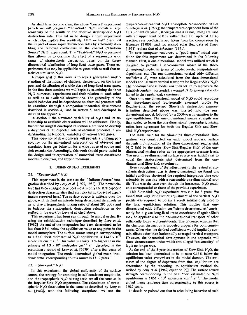
In comparing the behavior of the three N20 model experiments we first concentrate on the zonal mean structure. Figure 1 shows cross sections of zonal mean N20 mixing ratio from the Fast-Sink and Slow-Sink experiment for the months of January, April, July, and October as well as the January and July fields for the Slow-Sink experiment. The Regular-Sink experiment is not shown because its structure is midway between these extremes.

Many of the results displayed in Figure 1 show the same features already noted by Levy et al. [1979]: the upward equatorial bulge; pronounced meridional slopes of isolines, with steeper slopes present in the northern hemisphere at every comparable season; and pronounced downward depressions of lower values in the winter higher latitudes. In April and October the downward depressions show clearly the "lag" effect of the winter season in each hemisphere. Note also that the equatorial bulge shows some tendency to follow the sun's overhead position with some seasonal lag.

In the lower stratosphere and upper troposphere, Figure 1 shows a pronounced interhemispheric asymmetry, with smaller northern hemisphere than southern hemisphere values at corresponding latitudes during every month. This asymmetry was noted earlier in the tropospheric N20 study by Levy et al. [1982]. The explanation for this effect appears to be related to a surprising, but understandable, model phenomenon. Dynamical analysis of this model [Manabe and Mahl- man, 1976] shows a significantly higher eddy activity in the northern hemisphere stratosphere in comparison to the southern hemisphere. Associated with this extra eddy activity is a larger departure from radiative equilibrium and a net stratospheric radiative cooling in the northern hemisphere over the

annual cycle. This cooling is balanced by a very weak interhemispheric meridional circulation with hemispheric averaged vertical velocities of ,-• 3 km yr- • (,-• 0.01 cm s- •) (sinking in northern hemisphere). This differential mean vertical velocity of 6 km yr-• is sufficient to explain the model's interhemispheric N20 asymmetry. It remains to be determined whether or not this degree of asymmetry is present in the real atmosphere.

A comparison of the Fast-Sink against the Slow-Sink N20 fields in Figure 1 shows a very significant difference in the vertical gradients of N20 , with weaker gradients being associated with weaker destruction (Slow-Sink). Comparison of the 10 mbar meridional variations of N20 shows the strongest gradients in Fast-Sink N20. Its annual average north polar value is 68 ppbv, and the corresponding equatorial value is 141. In Slow-Sink N20 the north polar and equatorial annual mean 10 mbar values are 153 and 205 ppbv, respectively.

The above results indicate that a change in vertical gradient is associated with a concomitant change in horizontal gradient. This is visually obvious in Figure 1 by noting that the meridional slopes of the RN2 o surfaces are virtually unchanged over the two experiments shown at any given time of year. This observation, when combined with the predictable one- dimensional behavior already noted in sections 2.1 and 2.2, provides a means of predicting the behavior of a wide class of long-lived trace constituents independent of the magnitude of their vertical mixing ratio gradients. That is, if the nature of the stratospheric destruction (or production) is known, the global average vertical profile can be predicted with some accuracy using a simple one-dimensional model. Once this is known, the above information on the generalized meridional slopes of trace constituent isolines might be used to predict the latitude-height distribution (in principle, at least) for the zonal mean mixing ratio of the constituent of interest.

This prediction can be evaluated if real data is present in sufficient quantities. It is also possible that this approach can be used to evaluate possible measurement inaccuracies in the "observed" data set for similar trace constituents. We will address this in the next section.

The apparent validity of these relationships lends some support to the one-dimensional modeling approach of Wofsy [1976] in which the global model mixing ratios are spread out along "mixing surfaces," paralleling the observed tracer meridional slopes. However, a careful analysis shows that such slopes cannot be regarded as "mixing surfaces" but rather appear as a balance among competitive processes [-see Mahl- man et al., 1980, 1984]. Nevertheless, such a procedure could prove to be empirically useful, irrespective of the physical processes responsible for producing the equilibrium slopes.

As with most "general" relationships, there are limits to the useful range of application. It should not be expected to apply for a trace constituent which is far from its transport-chemical equilibrium. See, for example, the early evolution of the "In- stantaneous Source" experiment of Mahlman and Moxim [1978, Figure 5.1a]. Further, it should not apply for a trace constituent in which the production or destruction time scales are of comparable order (or shorter) to the time required for meridional or vertical exchange. An instructive example can be found in Figure 3.3 of Mahlman et al. [1980]. In the lower stratosphere the meridional slopes of ozone in that experiment are very similar to the N20 slopes seen here in Figure 1. This is because the chemical sources and sinks are essentially zero there for both modeled constituents. However, in the middle stratosphere the ozone isoline slopes are totally unlike the N20 slopes because the ozone production-destruction time scale is much faster than that of N20 destruction. In fact, the

2690 MAHLMAN ET AL.' SIMULATION OF STRATOSPHERIC N20

JANUARY FAST-SINK N20 (ppbv)

JULY FAST-SINK N:•O (ppbv) OCTOBE• FAST-SINK N20 (ppbv)

,o ::::::::::::::::::::: • ;<.:: • • :•...?...........•_.• • :..........• ...: .<•....... • • :: • :: • • • :: • :: • .•o '0::-.--:' •'---:--J :.•ii ::• i:-•'•-:.:-!::• •:: :-.....-• • i •?:. Z i. :./i ! i i i i •o : :.. :. :' :..... :•• • • i i '•.,'! i :.• •':. ::'.'• • :X• i ! i :• i.-Xi • ! • •-'•i :'• :• " ::::::::::- .::9•0:::::- ::! ::::::::•.!.u..:... ....... : ....... i!i'•,•::iiiiiiii•i• ' • :::• •'"' ""::: '•'••• -• .-ø•ii::::il •Ji :--".• :::::::::::-'"::::•:: '"":"::::' "::'• ::'""• •::' •::::::: :•'::::::'•

...... . . ........ .............

lO

$•o•:::::.•:::. :...____ ..•!:::::.. .:s :::::' ..::::::::::::::: ::::::::: ::::::::::::::::::::::::::::::::::::::: 90øN 60 ø 30 ø 0 o 30 ø • • • 6{) ø 30 ø 0 o 30 ø 60 ø 90øS

JANUARY SLOW-SINK N20 {ppbv) JULY SLOW-SINK N:zO {ppbv}

............ o •9o 2• 2s

38 . 250

ß g 65. •'•

• I ' ' ' • 990 • 90øN 60 ø 30 ø 0 o 30 ø 60 ø 90os 90ON 60 ø 30 ø 0 o 30 ø 60 ø 90øS

Fig. 1. Zonal mean N20 mixing ratio (ppbv) for January, April, July, and October for the Fast-Sink experiment and January and July for the Slow-Sink model experiment.

MAHLMAN ET AL.' SIMULATION OF STRATOSPHERIC N20 2691

N20 destruction is always so weak that midstratospheric mixing ratios are largest in the tropics, where the destruction rate is the fastest. We note that these chemical circumstances

which break the "constant slope" result are essentially the same as those qualitatively demonstrated by Mahlman [1975] to lead to species-dependent effective one-dimensional eddy diffusion coefficients for various modeled trace constituents.

We have not yet established, however, how slow the chemical destruction must be to retain the validity of this "constant slope" result. This question is examined carefully in section 4 and the appendix.

An additional examination of the model experiments shows that the above result can be generalized to three dimensions. The topography of surfaces of the time-averaged mixing ratio is essentially the same for all similarly long-lived trace constituents. This means that the local meridional and longitudinal slopes of time mean mixing ratio surfaces tend to be the same for trace substances in transport/chemical equilibrium as long as their source-sink chemistries are similar or are weak rela-

tive to transport. This property will prove useful for the analysis of N20 variability presented in sections 6 and 7.

3.2. Comparison With Observations

It is fortunate for this study that detailed measurements of long-lived species have been conducted by the National Oceanic and Atmospheric Administration (NOAA) Aeronomy Laboratory scientists at some selected geographical sites [Sch- meltekopfet al., 1977; Goldan et al., 1980]. Partly in support of the present study, these data have been analyzed in greater detail by J. T. Bacmeister et al. (unpublished manuscript, 1986) (hereafter referred to as BAM86). The measurements obtained include the ½hlorofluorcarbons CC13F and CC12F2 in addition to N20. This provides an opportunity to evaluate some of the "tracer slope" model results of the previous section.

Figure 2 shows the BAM86 annual mean N20 mixing ratio (in ppbv) at Laramie, Wyoming (41øN, 105øW). Also shown are annual mean vertical profiles at the same location from the three model experiments described in section 2. Note that the observed profile agrees closest with the Fast-Sink N:O experiment. Recall that the Slow-Sink N20 experiment is the one designed to reflect the best calculation of N:O destruction as of 1980. This destruction rate appears to be much too slow. Furthermore, recent observations of solar flux in the middle

N 2 0 AT LARAMIE

N 2 0 AT ANTARCTICA

110 -

190 -

315 -

500 -

685 -

o

15 z

-5

•20

MIXING RATIO (PPBV)

Fig. 3. Same as Figure 2, except at Antarctica (80øS, 120øW).

stratosphere [Frederick and Mentall, 1982] support a faster destruction rate than used in Slow-Sink N:O.

Given in Figure 3 are the summer (December-January- February) profiles of N:O at Antarctica (80øS, 120øW) (BAM86) and the model results for the three experiments at the same location and time interval. Again, the observed profile is most like that of the Fast-Sink N:O experiment. Note that the Antarctica mixing ratio decrease with altitude is rather similar to that of Laramie in Figure 2 for both model and observations.

Figure 4 shows the BAM86 combined averages for the Canal Zone (9øN, 80øW) and Brazil (5øS, 38øW). Here the samples were combined to enhance statistical significance. The three model experiments shown are from the model grid point encompassing the Canal Zone location. In this figure the observed profile is closest to that of Regular-Sink N:O.

While the "best" calculation of N:O as of 1980 is clearly too slow, all the discrepancies cannot be explained away by a judicious choice of the N:O removal efficiency in the three- dimensional model. Rather, for a given choice of tropical profile it is clear that the higher-latitude points of the model do not decrease with altitude rapidly enough. From another perspective the meridional slopes of the mean isolines of Rs2o are not as steep in the model (see Figure 1) as they are in the

110

190 -

315 -

500 -

685 -

- 35

15 z

-5

o MIXING RATIO (PPBV)

Fig. 2. Annual mean N20 mixing ratio (ppbv) profile at Laramie, Wyoming (41øN, 105øW) from BAM86 (heavy line). Also shown are model annual mean N20 profiles for the "Laramie" location from the •ast-Sink (F), Regular-Sink (R), and Slow-Sink (S) NeO experiments.

110 -

190 -

315 -

500 -

685 -

N 2 0 AT CANAL ZONE

o

15 z

-5

•20

MIXING RATIO (PPBV)

Fig. 4. Same as Figure 2, except at average of Canal Zone (9øN, 80øW) and Brazil (5øS, 38øW).

2692 MAHLMAN ET AL.: SIMULATION OF STRATOSPHERIC N20

observations. Roughly, the data suggest that the hemispheric mean observed meridional slopes are perhaps 30% steeper than those simulated by the model.

This result showing a model deficiency is surprisingly clear considering the severe geographical and temporal limitations of the observed data. The difference in slope shows up in the BAM86 CF2C12 data as well. This is a good example of how useful local data sets can be for three-dimensional model

evaluation. Discussion on the probable cause of this modeling discrepancy is given in section 5.

4. THEORETICAL INTERPRETATION OF MERIDIONAL

TRACER SLOPES

The simulated results showing strong similarities among the meridional slopes of N20 isolines for the three experiments leads us to pursue a more quantitative diagnosis of such behavior. In particular, we wish to examine the role of chemical destruction processes relative to that of dynamical mechanisms in determining meridional trace constituent slopes.

Briefly restated, the model experiments indicate that for sufficiently weak photodestruction chemistries, the spatial slopes of the time mean equilibrium mixing ratio isolines are essentially the same for all such long-lived trace constituents. The data of BAM86 shows clearly that this result is verified in the comparison of N20 and CF2Cl 2 slopes. However, the slopes of CFCl 3 are significantly flatter than those for N20 and CF2Cl 2. This implies that the destruction rate of CFCl 3 is sufficiently fast so as to impede the net dynamical tendency to establish similar time mean slopes for vertically stratified tracers.

How fast is sufficiently fast ? In an attempt to answer this in a straightforward way, a simple "two-slab" model is developed in the appendix. The simple model distills the insights offered by Mahlman et al. [-1984], Mahlman [1985], and Plumb and Mahlman [1986] on the essential processes governing the observed poleward-downward slopes of mean mixing ratio isolines in the lower stratosphere.

To a very crude approximation those results indicate that the two-dimensional equilibrium slope exists as a balance between zonal mean advection by the "diabatic" circulation and an effective meridional diffusion. This balance is used as a

basis for the governing equation to develop the two-slab model. It is given as equation (A1) in the appendix, along with more complete descriptions.

The use of the two-slab approximation (dividing the hemisphere into two equal area boxes) allows a straightforward solution to the simplified equations: a meridional structure (slope) part and a vertical structure of the horizontal average part (one-dimensional behavior). As demonstrated in the appendix, each of these solutions depends upon the nature of chemical processes in a readily understandable fashion.

We must point out here that this two-dimensional model should not be interpreted as a viable substitute for more complete two-dimensional transport parameterizations such as that given by Plumb and Mahlman [1986]. Rather, the goal is to isolate mechanisms determining the impact of chemical destruction processes on the global distribution of long-lived trace gases. A bonus from this analysis is that the relationship between one-dimensional and two-dimensional models is significantly clarified.

Because of the mathematical complexity of the analysis, the details of the two-slab model and its accompanying physical insights are presented in the appendix. The reader uninteres- ted in such details can skip the appendix and still examine the major implications of that development in the following two

paragraphs. For details and their implications for understanding one-dimensional and two-dimensional transport models, refer directly to the appendix.

The two-slab model of the appendix shows that the equilibrium poleward-downward slopes of mixing ratio isolines depend importantly on the photodestruction efficiency. Equa- tion (A36) shows that as the destruction efficiency increases, the meridional slope (•z/c•yR) flattens. However, for longer destruction times (inverse of destruction coefficient) greater than, say, 700 days, the meridional slopes are essentially independent of chemistry (see Figure A1). This result suggests that the slope prediction of Figure A1 can be tested against the results of the Fast-Sink and Slow-Sink N20 experiments. For the Fast-Sink experiment the tropical destruction rate (C) tr at 10 mbar is about 3.9 x 10 -8 s -• (•297 days). ((C) tr is the destruction parameter appearing in the slope equation (A36)). For the Slow-Sink N20 experiment, (C) '• is about 1.16 x 10- 8 s- • ( • 1000 days). The two-slab model results shown

in Figure A1 predict 10-mbar meridional slopes of -0.665 x 10 -3 and -0.855 x 10 -3, respectively, for a difference of about 22%. Comparisons of the actual slopes near 10 mbar for these two three-dimensional experiments show differences ranging from ,-• 15-25%. Thus this two-dimensional mechanistic model appears to capture the effect of faster chemistry on the three-dimensional model's meridional slopes. These predictions should be tested more carefully against available data and against three-dimensional model experiments using faster destruction rates, such as those for CFC13.

The second major conclusion of the appendix is that the effective global average eddy diffusion coefficient Kz depends indirectly upon the photodestruction coefficient in a predictable way (see Figure A1). In particular, equation (A32) shows that Kz depends directly upon the magnitude of the meridional slope (•z/c•yR). A plot of the predicted dependence of Kz on the tropical photodestruction rate is given in Figure A1. Thus in the two-slab model the effect of faster destruction chem-

istries is to slow down the global mean vertical tracer flux for a given mean gradient. How this variable Kz effect could change the ozone photochemical predictions for global one- dimensional models remains to be determined.

Both major conclusions gained from the two-slab model of the appendix thus refute the tentative implications of sections 2 and 3. Instead, (A32) and (A36) show the apparent "universality" of the meridional slopes and one-dimensional Kzs to be true only for rather slow destruction chemistries. The effect of faster chemistries is to flatten the meridional slope and therefore to reduce the effective one-dimensional K z value.

5. CAUSE OF THE "FLATTENED SLOPE" MODEL

DISCREPANCY

In section 3 it was shown that the meridional slopes of N•O isolines in the three-dimensional experiment were too flat by ,-•30% in comparison with available observations from BAM86. For understanding the biases of this model, as well as for designing future models, it is of interest to try to understand the cause of this discrepancy. The insights gained in section 4 and the appendix allow such an assessment.

The simple two-slab model given in the appendix suggests that the only significant mechahism leading to a slope- steepening effect is that of the diabatic (or similar) meridional circulation. Thus in the context of that simple model the three-dimensional model apparently needs a stronger meridional gradient of diabatic heating (more tropical heating and polar cooling).

This prediction is quite compatible with a well-known bias

MAHLMAN ET AL.' SIMULATION OF STRATOSPHERIC N :•O 2693

of this general circulation model (GCM) (e.g., see Manabe and Mahlman [1976]). The model polar regions (except summer) are significantly too cold relative to observations. Thus one can readily conclude that the model temperature fields are too close to their radiative equilibrium values [-see Mahlman and Umscheid, 1984]; therefore the magnitude of the model's meridional gradient of net diabatic heating is indeed to6 weak.

This is simply another verification of the often under- appreciated fact that the annual mean net diabatic heating of the stratosphere must ultimately be due to dynamical processes [Fels et al., 1980]. This perspective is compatible with the "transformed Eulerian" mean framework of Andrews and

Mcintyre [1976]. As shown, for example, by Andrews et al. [1983, equation (B13)], the role of tropospheric disturbances propagating into the stratosphere is to produce a convergence of "Eliassen-Palm flux," a measure of the net decelerative force produced by nonzonal disturbances. The decelerative effect produced by this zonal force acts to excite a "residual" circulation (which is qualitatively similar to the diabatic circulation), manifested by rising motion (and adiabatic cooling) in lower latitudes and sinking motion (and adiabatic heating) in higher latitudes. This high-latitude dynamical heating is balanced in the annual mean by net radiative cooling. Thus the stratosphere can be thought of as being driven from radiative equilibrium by the dissipation of tropospheric disturbances propagating into the stratosphere. Without such disturbances, the system would be very close to radiative equilibrium, with accompanying small values of net diabatic heating.

In the context of the transport discrepancy found in the three-dimensional model it can be concluded that the magnitude of the dynamical drive for this model stratosphere is somewhat deficient. The validity of this argument is already suggesteO in the present model in the sense that the northern hemisphere isoline slopes are noticeably larger than the equivalent southern hemisphere slopes (see Figure 1). This is compatible with the observation that the northern hemisphere of this model is considerably more dynamically active than its southern hemisphere [see Manabe and Mahlman, 1976].

These arguments strongly indicate that improvement of this discrepancy is directly dependent upon a solution of the "cold- bias" deficiency of these models. Experience with N20 modeling in more recent versions of the GFDL "SKYHI" GCM [e.g., Mahlman and Umscheid, 1984] has already shown these arguments to be essentially correct; as the cold bias is reduced, the meridional N20 slopes become steeper.

6. VARIABILITY OF STRATOSPHERIC N20

6.1. Longitudinal Variability

In previous N20 modeling studies we have investigated the spatial and temporal variations of N20 in the troposphere [-Levy and Mahlrnan, 1980; Levy et al., 1982]. Here we examine the nature of stratospheric N:O variations and their meteorological and statistical interpretation. Such an analysis can prove to be of much theoretical and practical value.

As in the work by Levy et al. [1979], we define the longitudinal (percent) standard deviation as •

100

U = - where ( ) x is the zonal mean.

Figure 5 shows meridional cross sections of Vx for the months of January, April, July, and October for the Fast-Sink and January and July for the Slow-Sink N20 experiments. In this figure, Vx shows very similar structure to that given by

Levy et al. [1979]. In particular, as Levy et al. pointed out, the largest values of V x appear in those regions where the vertical gradient of (R) '• is the largest. Thus values of the order of 10% appear in the stratosphere, while tropospheric values are less than 1% (much less in the tropics). This wide range in variability for a particular global lifetime demonstrates a serious limitation of the Junge [1974] rule relating variability to global lifetime. The association of variability and mean vertical gradient has been made in a more specific and usable way by Ehhalt et al. [1983] for temporal variability. This will be addressed in detail later.

Comparison of the N20 results in Figure 5 shows that the Fast-Sink Vxs are about twice as large as those of the Slow- Sink Vxs (actual range • 1.5-2.7). These results suggest a simple modification of the Junge [1974] rule. A particular form of variability (V,• here) and the global lifetimes for two trace gases a and b have the following approximate relationship for local variability'

Vx(a ) z(b) c (2)

Vx(b) r(a)

where r represents global lifetime (global amount/global chemical destruction) and C is a constant of order 1. Empiri- cally, here the best fit that encompasses the model data is C • 1.15 _+ 0.35 (As r(a)--} r(b), we expect C--} 1.). Thus (2) can be thought of as a modified Junge rule but one which retains its extremely simplified character. The limitations of such a simple-type rule will be investigated in the next section.

6.2. Temporal Variability

We now turn toward the problem of understanding the temporal variations of long-lived trace gases. Perhaps the simplest statistical quantity is the temporal (percent) standard deviation Vt, where

100

V, = (--• [((R -- (R)t)2)'] •/2 (3) and ( )t is the time average over an arbitrary interval.

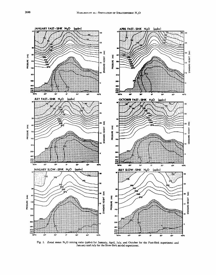
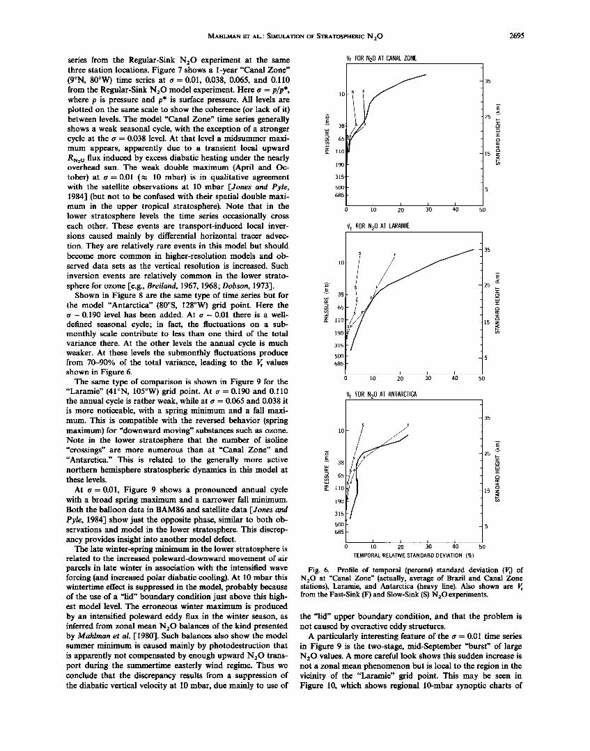
Shown in Figure 6 are annual N20 V, from BAM86 for "Canal Zone" (actually an average of Brazil and Canal Zone), Laramie, and Antarctica compared to the same quantity from model grid points corresponding to these locations for the Fast-Sink and Slow-Sink N20 experiments. Generally, Figure 6 shows that the "observed" V,s are greater than the Slow-Sink and Fast-Sink model values. Exceptions to this occur in the lower stratosphere at Canal Zone and Antarctica.

At this time we can only speculate on the cause of these discrepancies. The BAM86 tropospheric V•s appear to be too large relative to other studies. Whether this is a precision error problem or an analysis inconsistency remains to be determined. The smaller •s relative to BAM86 observed near 10 mbar are probably related to the model's too slow decay of N20 with altitude, especially in mid-latitudes (for further analysis, see section 6.3). It is also possible that vertical velocity fluctuations in the model are suppressed at 10 mbar by the "lid" bo?ndary condition. In addition, measurement errors could be adding significant contamination near 10 mbar. Fi- nally, the better agreement in V, near 50 mbar at Antarctica is likely to be fortuitous as a result of insufficient sampling at this site. Both (R) • and V, exhibit fluctuations in the vertical at Antarctica that seem to be related to insufficient sampling (BAM86).

In order that future observational analysis efforts may have some rough guidance on the type of variability to be expected at a given station location, we next present stratospheric time

2694 MAHL•AN ET AL.: SIMULATION OF STRATOSPHERIC N20

JANUARY FAST-SINK V x (%)

90ON 60 ø 30 ø 0 o 30 ø 60 ø

10 -30

-25

38-

-20 •' '"" •E 65-

-15 • • 11o-

•Z •- 190- -10 •

315-

500- 5

685-

835- 940- 99•

•0os

z

60 ø 30 ø 0 o 30 ø 60 ø 90øS

JULY FAST-SINK V x (%)

"•' '"• 25 38 :

...... 190-

• -•0

500- -5

835- • 940- • 990

90ON 6• ø 30 ø 0 o 30 ø 60 ø 90ø5

OCTOBER FAST-SINK V x (%) 10

38-

•'E 65- • 110-

• 190- 315-

500-

685-

835- 940- 990

90øN

5

60 ø 30 ø 0 o 30 ø 60 ø 90os

JANUARY SLOW-SINK Vx (%) JULY SLOW-SINK Vx (%)

'"' o '"' • • • 11o. "'

,,o .,• • •':••:•:.- • ,,o•11..:...::.......:•i7 •//.: :'•,'•'• • • • ,,o .

::::: ........ ::.02::::::.'": 5

835 ......... :'-.::'.:: ......

90ON 60 ø 30 ø 0 o 30 ø 60 ø 90os 90øN 60 ø 30 ø 0 o 30 ø 60 ø 90ø$

Fig. 5. Longitudinal (percent) standard deviations (V•) of NaO for January, April, July, and October for the Fast-Sink experiment and January and July for the Slow-Sink model experiment.

MAHLMAN ET AL..' SIMULATION OF STRATOSPHERIC N 20 2695

series from the Regular-Sink N20 experiment at the same three station locations. Figure 7 shows a 1-year "Canal Zone" (9øN, 80øW) time series at a--0.01, 0.038, 0.065, and 0.110 from the Regular-Sink N20 model experiment. Here a -- p/p*, where p is pressure and p* is surface pressure. All levels are plotted on the same scale to show the coherence (or lack of it) between levels. The model "Canal Zone" time series generally shows a weak seasonal cycle, with the exception of a stronger cycle at the a = 0.038 level. At that level a midsummer maximum appears, apparently due to a transient local upward RN2o flux induced by excess diabatic heating under the nearly overhead sun. The weak double maximum (April and Oc- tober) at • = 0.01 (• 10 mbar) is in qualitative agreement with the satellite observations at 10 mbar [Jones and Pyle, 1984'1 (but not to be confused with their spatial double maximum in the upper tropical stratosphere). Note that in the lower stratosphere levels the time series occasionally cross each other. These events are transport-induced local inversions caused mainly by differential horizontal tracer advection. They are relatively rare events in this model but should become more common in higher-resolution models and observed data sets as the vertical resolution is increased. Such

inversion events are relatively common in the lower stratosphere for ozone [e.g., Bredand, 1967, 1968; Dobson, 1973].

Shown in Figure 8 are the same type of time series but for the model "Antarctica" (80øS, 128øW) grid point. Here the a = 0.190 level has been added. At a = 0.01 there is a well-

defined seasonal cycle; in fact, the fluctuations on a submonthly scale contribute to less than one third of the total variance there. At the other levels the annual cycle is much weaker. At these levels the submonthly fluctuations produce from 70-90% of the total variance, leading to the V, values shown in Figure 6.

The same type of comparison is shown in Figure 9 for the "Laramie" (41øN, 105øW) grid point. At a = 0.190 and 0.110 the annual cycle is rather weak, while at a = 0.065 and 0.038 it is more noticeable, with a spring minimum and a fall maximum. This is compatible with the reversed behavior (spring maximum) for "downward moving" substances such as ozone. Note in the lower stratosphere that the number of isoline "crossings" are more numerous than at "Canal Zone" and "Antarctica." This is related to the generally more active northern hemisphere stratospheric dynamics in this model at these levels.

At a- 0.01, Figure 9 shows a pronounced annual cycle with a broad spring maximum and a narrower fall minimum. Both the balloon data in BAM86 and satellite data [Jones and Pyle, 1984] show just the opposite phase, similar to both observations and model in the lower stratosphere. This discrepancy provides insight into another model defect.

The late winter-spring minimum in the lower stratosphere is related to the increased poleward-downward movement of air parcels in late winter in association with the intensified wave forcing (and increased polar diabatic cooling). At 10 mbar this wintertime effect is suppressed in the model, probably because of the use of a "lid" boundary condition just above this high- est model level. The erroneous winter maximum is produced by an intensified poleward eddy flux in the winter season, as inferred from zonal mean N:O balances of the kind presented by Mahlman et al. r1980'1. Such balances also show the model summer minimum is caused mainly by photodestruction that is apparently not compensated by enough upward N:O transport during the summertime easterly wind regime. Thus we conclude that the discrepancy results from a suppression of the diabatic vertical velocity at 10 mbar, due mainly to use of

V FOR N20 AT CANAL ZONE

lO

E • 38[

• •o

190

315 -

500 •

685 -

0 I I I , 1

10 20 30 40 50

V t FOR N20 AI LARAMIE

15 z

65

•o

190

315

500 -

685 -

I i J • . J 0 lO 20 30 40 50

V t FOR N20 AT ANTARCTICA

sF

5500 • -- 685

15 z _

5

15 z

0 10 20 30 40 50

TEMPORAL RELATIVE STANDARD DEVIATION (%)

Fig. 6. Profile of temporal (percent) standard deviation (Vt) of N20 at "Canal Zone" (actually, average of Brazil and Canal Zone stations), Laramie, and Antarctica (heavy line). Also shown are V t from the Fast-Sink (F) and Slow-Sink (S) N20 experiments.

the "lid" upper boundary condition, and that the problem is not caused by overactive eddy structures.

A particularly interesting feature of the a -- 0.01 time series in Figure 9 is the two-stage, mid-September "burst" of large N:O values. A more careful look shows this sudden increase is not a zonal mean phenomenon but is local to the region in the vicinity of the "Laramie" grid point. This may be seen in Figure 10, which shows regional 10-mbar synoptic charts of

2696 MAHLMAN ET AL.' SIMULATION OF STRATOSPHERIC N :,O

300

275

250

225

200

175

150

125

100

75

5O

CANAL ZONE

I I I I I I I I I I I

J F M A M J J A S O N D

Fig. 7. One-year model N20 time series from the Regular-Sink N20 experiment for "Canal Zone" (actually, average of Brazil and Canal Zone stations) at model a levels 0.01, 0.038, 0.065, and 0.110. Here a -- p/p* where p is pressure and p* is surface pressure.

0'=.110

0':.065

0'=.038

0':.010

RN2O and model streamlines for the model dates of September 6, 10, 14, and 18. During this period the weak summertime circulation is giving way to the stronger, planetary wave- dominated winter westerlies. Accompanying this transition, an anticyclone forms over the eastern United States. Associated with this formation, a region of tropical N20 values is drawn poleward over the western United States. Figure 10 for Sep- tember 10 shows larger N20 values moving into the western United States as a result of this transient disturbance. These

larger N20 values are sustained over the western half of the United States until an even larger N20 burst appears on Sep- tember 18, associated with more southerly flow as the anticyclone over the eastern United States reintensifies. This burst of N20 is transported irreversibly into mid-latitudes and is associated with transient growth of the subtropical anti-

cyclones separating tropical easterlies from mid-latitude westerlies.

Presently, the observed local N20 data are not good enough to verify or disallow the occurrence of such phenome- na in the actual atmosphere. However, the nature of this model phenomenon is such that there is no reason not to expect such transport events to occur in the real atmosphere as well. Depending on its spatial scale, a specific event may or may not be visible from satellite data. The event described here would be just below the sampling resolution of a typical polar-orbiting satellite (,-, 30 ø longitude).

6.3. "A" Diagnostics

Recently, Ehhalt et al. [1983] expanded upon the observation that tracer variability tends to be largest in regions of

ANTARCTICA

[ I I I I I I I I .... I i ', 300 1.^,.•,• '• •'•"•' .... • '• . 7. .... • .... ,•,•/•Vl• .• ,h,,', - ".,, ' ',',• -., ' , '•. • J•=.190 275 v ' 5 ' •j .... _

200

175 •=.0•8 150

75

50 J F M A M J J A S O N D

Fig. 8. Same as Figure 7, except at the model grid box corresponding to Antarctica (80øS, 120øW).

MAHLMAN ET AL..' SIMULATION OF STRATOSPHERIC N20 2697

300

275

250

•' 225 200

•C• 175 • •5o

o• 125

z looJ J

LARAMIE

Fig. 9.

I I I I I I I I I I

M A M J J A S O N D

Same as Figure 7, except at the model grid box corresponding to Laramie, Wyoming (41øN, 105øW).

largest vertical tracer gradient [e.g., Levy et al., 1979]. They defined a new quantity, the "equivalent displacement height,"

[((R - (R)'):)'] A = (4)

Thus A is simply the temporal standard deviation divided by the time mean vertical gradient. Alternatively, it can be defined as Vt/8 In (l•t)/Sz.

Shown in Figure 11 are N20 A values calculated for Laramie, Wyoming, from BAM86 and from the three N20 experiments described here. These A values have been compared against As for the same conditions from the "Slow- Destruction" three-dimensional ozone model experiment of Levy et al. [19851. The results are very similar to those of Figure 11; an exception appears at 10 mbar, where the ozone chemistry is very fast. Thus the model shows an even stronger agreement of As than that given in the more limited data sets used by Ehhalt et al. [1983]. We conclude that their original assertion on the usefulness of A is indeed correct. Fur-

thermore, Figure 11 shows that the model A values agree reasonably well with the As from the BAM86 analysis. In each case, A has a minimum of about 1 km in the lower stratosphere, rising to several kilometers in the upper troposphere and in the middle stratosphere. The striking agreement of the model As with the observational results of BAM86 suggests strongly that the model Vt deficiency shown in Figure 6 arises mainly from the model's excessively weak vertical gradients at Laramie (too weak meridional slopes).

Note also that the A values in Figure 11 are not identical, even for the "perfect" model data. The three N20 experiments are very similar, but the midstratospheric As for the Fast-Sink N20 are generally smaller than for Regular-Sink and Slow- Sink N20. The largest A values are found in Slow-Sink N20. These small but systematic differences in A for different trace constituents lead us to seek an explanation for such differences.

7. THEORETICAL INTERPRETATION OF "A"

STATISTICS

The numerical results of section 6 show small but noticeable

differences in A magnitudes for different modeled N20 de-

struction scenarios. Because of the availability of detailed re- suits from the three-dimensional model as well as insights from the previous analyses in this paper, we offer a different perspective on the significance of A than that given by Ehhait et al. r 1983]. In particular, we emphasize the factors leading to differences in A for different trace constituents.

First, we write the general trace constituent continuity equation in log pressure coordinates as

8R __- _V3 ß V3R + V 2 ß K H V2R

1 8 + • psK,; + SMS (5)

where the log pressure coordinate and associated variables z and Ps are defined as in the appendix, Kn and K v are horizontal and vertical subgrid-scale diffusion coefficients used in the three-dimensional model, V3 and V3 the three-dimensional vector velocity and gradient operator in log pressure coordinates, V2 the horizontal gradient operator and SMS is the net of all chemical/physical sources minus sinks.

Multiplying (5) by R'= R- (R) t and time averaging, we obtain the trace constituent eddy variance equation

+ (R'V•. KnVR'}' + • psK, • R' + (R'SMS' (6) In (6) the right-hand side terms from leR to right are the temporal variance production, the variance advection by mean and transient motions, the horizontal variance dissipation, the vertical variance dissipation, and the variance production or dissipation by chemical changes (usually dissipation), respectively.

It is worth noting that the conceptual model developed below is fundamentally different from the usual mechanistic approaches [e.g., Plumb, 1979]. In that type of development the transient tracer R' is viewed as evolving in time from a small amplitude perturbation on a time mean background state. In this work we visualize the transient tracer field as

2698 MAHLMAN ET AL.' SIMULATION OF STRATOSPHERIC N 20

lomb N20 MIXING RATIO (ppbv) SEPT.6 •oN 'iii'ii:::iiiiiii.::•iiii:•..'iii!i!!:.:i•'-:.' '":i i!i!i:::•: .... "::

I:: :-: :. :• t.'.ø..•• i i i i i ili i• i iii i :: i• ...../...:• • :•i :: i ! i i i :: i i i i i i i ..."... /

1800W 150 ø 120 ø 900 •00

lomb N20 MIXING RATIO (ppbv) SEPT.10

72øN i• "• ......... -(• ................................... :

.... "'••2ø2• v•-'-'•::::::::::" '•'/ 30 o- 130

EQ . 180øW 150 ø 120 ø 90 ø 60 ø 30øW

lomb N20 MIXING RATIO (ppbv) SEPT. 14 72øN

60 ø -

30 o-

72øN

60 ø -

30 o.

EQ.

180øW 150 ø 120 ø 90 ø 60 ø 30ow

lomb N20 MIXING RATIO (ppbv) SEPT. 18

lomb VECTOR STREAMLINES SEPT. 6

...... ß •• •--•• - . ....... 30 ø

180øW 150 ø 120 ø 90 ø 60 ø 30ow

lomb VECTOR STREAMLINES SEPT. lO 72øN

•••-'-•, •; __J_• (', ,,/"!.-,4-J...•.-d___:• 600

................. •. .

180øW 150 ø 120 ø 90 ø 60 ø 30ow

lomb VECTOR STR•MLINES SEPT. 14

• -- . 30 ø

180øW 150 ø 120 ø 90 ø 60 ø 30ow

lomb VECTOR STR•MLINES SEPT. 18 72ON

60 ø

30 ø

•:Q 180øW 150 ø 120 ø 90 ø 60 ø •30øW 180øW 150 ø 120 ø 9-0 ø 60 ø 30ow

Fig. 10. Instantaneous 10-mbar charts of N20 mixing ratio (left, ppbv) and wind vector/streamlines (right). Each wind barb equals 10 ms-•. Dates shown are for September 6, 10, 14, and 18. Small "L" marks Laramie location.

being ever present at nonnegligible amplitude. Accordingly, the approximate long-term balance is between production/advection of transient variance and its dissipation. For time-averaged statistics the temporal evolution term in (6) is negligible.

Now we proceed by introducing the following definitions:

(R'V2 ß Ki-iV2R')t + ((R'/ps)t•/t•z psK,, (t•R'/t•z)) t C m = (R,2)t (7)

(R'SMS') t

Ca • (•,•), (8)

Here C m - 1 can be thought of as a mechanical dissipation time and Cc- • as a chemical-damping time. These quantities, Cm and Cc, can be visualized as being computed in advance by the three-dimensional model for a given trace constituent. A priori, there is no proof that Cm, let along Cc, should be the same for different trace constituents. Nevertheless, we make conceptual progress by condensing these intrinsically difficult terms, substituting (7) and (8) into (6) to obtain

c3t 2 -- (V3'R')t' V3(R)t- V3' V3 • --(C m -Jr- Cc)(g'2) t (9)

MAHLMAN ET AL.' SIMULATION OF STRATOSPHERIC N •.O 2699

DELTA FOR N20 AT LARAMIE

a_ 110

190

315

5OO

685

35 F RS

MODEL

i I I

2 5 7 10

SCALED DISPLACEMENT LENGTH (km)

Fig. 11. Annual mean N20 "A" profile (scaled displacement length) at Laramie, Wyoming (41øN, 105øW) from the BAM86 analysis (For definition, see (4)). Also shown are model N20 A profiles for the "Laramie" location from the Fast-Sink (F), Regular-Sink (R), and Slow-Sink (S) N20 experiments.

At statistical equilibrium (or with sufficiently long time averaging), (9) becomes

--(V3'R') t ß V3(R) e-- (V 3 ß V3(R'2/2)) ' ' =

Cm + C•

The first term in the numerator of (10) is the familiar production of temporal variance by a net transient flux of R down the time mean gradient of R. The second term represents the average advection of transient variance into a given region by mean and transient winds. Roughly speaking, if upstream of a chosen point is a region of large production of (R':)', the tendency of this R': to be "blown downstream" would act to increase the local transient variance. Conversely, if the upstream area is a quiet one in terms of transient variance production, then this advection would act to decrease the local variance. Thus this term can readily be either positive or nega- tive, depending on location. Here we will simplify the treatment of this term by considering only the advection of temporal variance by the time mean state (or equivalently, that the triple product term in equation (10) is negligible). Also, we will assume for convenience that the spatial gradients of are small relative to spatial gradients of (R'2) t. These assumptions lead to essentially the same result as using linear theory directly to derive (10).

Now working on the first term in (10), we note that the only transient eddy flux of R of interest here is the statistically averaged component normal to the gradient of (R)'. Accord- ingly, we describe this statistical quantity (generated explicitly by the three-dimensional model) as an effective symmetric diffusion process. We thus assume that locally

(u'R')t=--Kx* &-•• (v'R')t=--KY* c3y ß c•(R )' (11) (w'R')' = --K:

•z

Note that these K*s are not the same as the subgrid-scale coefficients used in the three-dimensional model, nor are they at all similar to the effective Ks defined in the appendix. Here these K*s represent the net statistical effect of transient motions to transfer R down its time mean gradients. The actual physics of this process is an extremely complicated mix of advective processes setting up diffusive processes and can only

rationally be attacked in a reasonably high-resolution three- dimensional GeM (if then !). Note, in principle, that these K*s can vary for different trace constituents.

We now substitute the definitions (11) into (10), divide by (•(R)e/•z) 2 and use the simplifications indicated above to obtain

A 2 = (R'2) ' [(c•(R)e/cqz)]2 • Kx*E(c•z/cqx<R>,)] 2 + K•,*E(c•z/cqY<R>,)]2 -Jr- Kz* --«(V3> t' V3(A 2) + '" (C m -Jr- Cc) -1 (12)

In (12) we have used the definitions

c3z (c3(R)7t•y) c3z (•(R)t/•x) - - (13)

C3y(R), (c3(R)t/c3z) C•X<R>,

which, similar to the appendix, define the time mean slopes of equilibrium trace constituent mixing ratio surfaces.

The quality A in (12) is the same as that defined by Ehhalt et al. [1983]. Thus we are now in a position to investigate more carefully why A, the "equivalent displacement height," exhibits such useful properties. Furthermore, it allows us to carry into the time domain our effort in this paper to predict future trace constituent behavior on the basis of a small number of GeM

integrations to statistical equilibrium. Inspection of (12) tells us that if trace constituents a and b

are: (1) almost chemically conservative (Cc << C,•), (2) have the same effective K's, (3) have the same (R)' "topography," and (4) omitted higher-order terms are negligible, then

Aa 2 -- Ab2

provided we further note that if the As are equal, then the advection of As in (12) would also be equal.

The above arguments provide an explanation for why A is essentially the same in the lower stratosphere for the three model experiments, as shown in Figure 11. In that altitude range, Cc•0 and the "topography" of the (R) ' surfaces is essentially identical, as pointed out in section 3. Further, we expect the K*s to be more or less the same for different trace constituents as long as the chemistry is sufficiently slow (and perhaps the mechanical dissipation of R variations has the same character for each trace gas).

Inspection of (12) also justifies the caution of Ehhalt et al. [1983] in interpreting A literally as a vertical displacement, as might be superficially inferred from the vertical gradient dependence. As shown in the appendix, the equilibrium tracer slopes represent a tight coupling between horizontal and vertical transport/chemical processes. Evaluation of (12) and the basic components of (--V3'R') t. V3(R) t from the GCM suggests a crude isotropy in the production of A2; the east-west and north-south tracer slopes approximately compensate for the large differences in effective K*s (Kx* > Ky* >> K:*). An- other way to illustrate this is to redefine a A leading to (12) by dividing by the meridional gradient (c•(R)t/c•y). In this case the modified As so produced have magnitudes of ,-• 1000 km. Therefore we conclude that A should be thought of as a "scaled displacement length," because the definition of A carries no implications of dominance of displacement from one coordinate direction over another. However, "equivalent displacement height" remains an appropriate description for A as long as it is recognized that transient R perturbations can come from any coordinate direction with more or less equal probability for a tracer in statistical equilibrium.

Next we explore circumstances under which Aa is predicted to be different than At,. First, in (12) if Cc > C,,, it would have a direct damping effect on the calculated A as a result of this accelerated temporal variance destruction. Superficially, this is

2700 MAHLMAN ET AL.' SIMULATION OF $TRATOSPHERIC N 20

a rather weak constraint, since Cm-• ~ 10--20 days (at least in this GCM for the lower stratosphere). Thus two trace constituents, one with Cc-•~ 50 days and one with Cc-•= 500 days, would appear to be predicted to exhibit very nearly the same A value. However, this apparently is not the case. Even slower chemical destructions enter the problem indirectly through their influence on the equilibrium R slope appearing in the numerator of (12). The theoretical model of the appendix (as illustrated in Figure A1) shows that significant tracer slope flattening is expected for chemical destruction times ranging from ~ 1 0-1000 days.

Thus the combined analyses of the appendix and (12) predict an observable decrease in A for a "shorter" long-lived trace constituent such as CFC13, relative to other gases such as N20 or CF2C12. The physical interpretation of this predicted A reduction for gases such as CFC13 is straightforward in the sense that as the equilibrium (R) t surfaces become flatter, the opportunity for horizontal displacements to contribute to A become reduced.

Finally, as the chemical destruction becomes fast.relative to Cm, it is likely that the K*s and the gradients of A 2 in (12) would also change. At this fast destruction limit it is not presently possible to predict the influence these additional processes would have on the determination of A.

The predictive capability implied in (12) has been tested in the three-dimensional model for the Fast-Sink and Slow-Sink

experiments, using the •20% Fast-Sink reduction in slope between 38 and 10 mbar, as noted at the end of section 3.2. This calculation predicts that Fast-Sink N20 at Laramie over this layer should have a A of about 15% lower (for a factor of 3 increase in photodestruction rate) than that for Slow-Sink N20. The actual difference in the three-dimensional model is about 20%. Given the crudeness of the calculations, this agreement is rather close.

The above prediction of a reduced A for long-lived gases with faster-destruction times was also tested in the observa-

tional study of BAM86. Unfortunately, their results were in- conclusive. If anything, the A values for (faster destruction) CFC13 might be greater than for CF2C12 and N20. However, they point out that the sampling error for calculation of A is so large (especially for CFC13) that no statistically significant identification of A differences can be made from their data set.

Thus the prediction of small, but illuminating, differences in A statistics must await more complete data sets with higher- precision measurements.

Finally, we note the possibility of circumstances in which the simple equilibrium A 2 model of (12) may be inappropriate. For short sampling intervals or circumstances following seasonal transitions the assumptions leading to (12) may not hold.

An important example of such a possibility is given by Hess and Holton ['1985]. They address the relatively large A 2 values measured by Ehhalt et al. [1983] for summer mid-latitudes. Using a mechanistic model, they hypothesize that the relatively large A 2 values are "frozen" in the zonal flow following the large meridional exchange near the descending zero zonal wind line associated with the transition to summertime east-

erlies (e.g., see Dickinson [1969]' Mahlman and Moxim [1978]). These large tracer perturbations thus get caught in the easterly flow and are simply advected zonally.

Such a localized circumstance suggests a more complex interpretation of the framework given in (6)-(12). During the zonal wind reversal, A 2 values would be increased substan- tially as a result of enhancements of the variance production terms. In the summertime easterlies, both production and dis-

sipation C,, are rather weak; the high A 2 values are simply advected past a point by the zonal easterly flow. For such a short period the direct balance between production and dissipation controlling the A 2 amounts in (12) is not realized. However, for annual statistics the balance in (12) should be a good approximation.

8. SUMMARY AND CONCLUSIONS

In this paper we have described three stratospheric N•O experiments using the GFDL general circulation/tracer model. The first experiment (Regular-Sink N:O) uses stratospheric photodestruction coefficients thought to be correct in the mid- 1970's. The second experiment (Slow-Sink NeO) uses the temperature-dependent absorption cross sections introduced by Selwyn et al. [1977] as well as other chemical data current in 1980. However, this choice produces too much NeO in the middle stratosphere. To investigate the possibility of the modeled stratospheric N20 losses being too weak, a third experiment (Fast-Sink N20 ) was run which uses doubled values of the photodestruction coefficients from the Regular-Sink N20 experiment.

The three N20 three-dimensional model experiments have been compared in detail against the detailed observational analysis of J. T. Bacmeister et al. (unpublished manuscript, 1986) (BAM86). In terms of one-dimensional structure, the observations are most like a model somewhat midway between the Regular-Sink and Fast-Sink N20 experiments. This suggests the possibility of required faster N20 removal, as indicated by the inferences of lower O2 absorption cross sections by Frederick and Mentall [1982].

Integration and analysis of these three N20 experiments revealed some interesting behavior. It was found that the Fast- Sink and Slow-Sink N20 experiments exhibit predictable globally averaged (one-dimensional) behavior, given the results from the Regular-Sink N20 experiment. Specifically, the set of global one-dimensional eddy diffusion coefficients (K•s) producing consistent globally averaged behavior for one experiment were found to produce excellent predictions of the one- dimensional behavior of the other two experiments. Fur- thermore, it was found that the meridional slopes of N20 isolines are virtually identical in the lower stratosphere for the three N20 experiments.

The generality of the above two results was investigated through use of a simple theoretical two-slab model. In this model the transport balances leading to equilibrium meridional mixing ratio slopes are solved explicitly. Specifically, the simple model shows that meridional mixing ratio slopes are the same for a wide class of trace constituents, given a very slow destruction (or production) chemistry. For gases with moderate to fast photodestruction rates, the effect is to flatten the meridional slopes.

In addition, the two-slab model shows a physical basis for the one-dimensional global eddy diffusion coefficient K•. In this model, K• depends upon the meridional slope of a given constituent (which in turn depends upon the chemical destruction rate). Also, Kz depends upon the intensity in which upward propagating disturbances from the troposphere force the stratospheric zonal winds. Finally, the two-slab model shows that the meridional isoline slope in turn depends upon the Kz value, although in most cases the dependence is com- paratively weak. The two-slab model thus predicts that the apparent "universality" of meridional slopes and Kz for N20 fortuitously arise from the relative weakness of the prescribed destruction chemistries. Tracers with stronger chemistries are predicted to exhibit noticeably different behavior. Conse-

MAHLMAN ET AL.' SIMULATION OF STRATOSPHERIC N2 ̧ 2701

quently, this simple theoretical model can be used to predict meridional slopes and effective one-dimensional Kzs for a wide class of longer-lived trace gases.

Comparison of the model meridional mixing ratio slopes against the climatologies of BAM86 indicate that the model slopes are too flat by about 30%. By using the predicted slope structure from the simple two-slab model we infer that the basic cause of this deficiency is a too weak dynamical forcing of the zonal winds in the model stratosphere. This leads to a situation in which the polar temperatures are too cold, and the model temperatures are too close to their radiative equilibrium limits. Thus we conclude that this discrepancy has the same roots as that of the well-known polar cold bias of this and other GCM's.

A detailed comparison of the model's temporal variability has been made against the BAM86 N20 climatology. Gener- ally, model and observation show reasonable agreement except near 10 mbar, where the observed variabilities are significantly larger, and the higher-latitude seasonal cycle is out of phase. The model temporal standard deviations have been divided by the time mean vertical mixing ratio gradient to yield a quantity "A." This A has been shown by Ehhalt et al. [1983] to reveal a remarkable unity among a wide class of constituents. This model essentially verifies the wide range of applicability of using A statistics.

A simple theoretical model has been developed which shows why A statistics are so often similar for different trace gases. Also, the simple model offers specific predictions of the conditions under which As should differ among various trace constituents. These predictions agree with the three-dimensional model behavior but may disagree with the BAM86 observations. Unfortunately, the observed data are not good enough to isolate any meaningful statistical significance. Thus a full test of this prediction awaits further observations and analysis.

Finally, detailed profile time series are presented from the model for those station locations used in the BAM86 observa-

tional analyses. These time series, along with supporting model horizontal charts, show a complex behavior with pronounced seasonal cycles, local transport induced "inversions," and detailed meridional transport events associated mainly with seasonal transitions and transient disturbances. Such

time series, in addition to the other model results, can allow an evaluation of the sampling required for studies such as BAM86 to resolve fuller details of the local climatologies of various long-lived trace gases.

APPENDIX: A SIMPLE MODEL FOR ASSESSING THE

INFLUENCE OF CHEMISTRY ON MERIDIONAL

TRACER SLOPES AND VERTICAL

TRANSPORT

In section 3 it was shown for this model that suitably long- lived trace gases all exhibit the same equilibrium poleward- downward slopes of mean mixing ratio isolines. The observational study of BAM86 showed this to be true for N20 and CF2C12. However, the mean slope for CFC13 is flatter than those of the other two, apparently because of the faster photodestruction chemistry appropriate for CFC13.

The purpose of this appendix is to develop a simple model that isolates the essential physical processes leading to equilibrium tracer slopes in the presence of chemical destruction. Here we have in mind the rather large class of atmospheric trace constituents characterized by a tropospheric source and a stratospheric destruction. To accomplish this, we introduce a two-slab model which breaks the meridional plane into two equal-area regions, 0-30 ø and 30-90 ø latitude. Here ( )t,

represents a spherical coordinate average over the "tropical" slab and ( )hl is the average over the "high-latitude" slab. The meridional distance between slabs and across slabs is

chosen to be a single, spherical geometry consistent value y. With this we can utilize a Cartesianlike model, while incorpor- ating the important aspects of the spherical geometry. In this model the hemispheric average is given by ._[_( )hi].

Now consider the simplest possible model that captures the essence of the basic processes controlling the meridional slope of zonal, time mean isolines of tracer mixing ratio. Following the physical model of Mahlman et al. [1984], in isentropic coordinates the structure of trace constituent transport in the meridional plane can be thought of crudely as a balance between an advection by the diabatic circulation [Dunkerton, 1978] (ultimately forced by dissipating tropospheric disturbances) and a meridional diffusion (caused by the same tropospheric disturbances) (see also Holton [1980]). For a more detailed numerical justification, see Mahlman [1985]. In this ultrasimplified form, the two-dimensional trace constituent continuity equation can be written as

•(R) ;• •(R) ;• •(R) ;• -

1 • •(R) • + Ky cos C(y, z)(R) • (A1)

a cos • • a34

where ( )x is a zonal average, a is the earth's radius, K• is an effective meridional diffusion coe•cient, and C is a photodestruction coe•cient which, in general, varies with latitude and height. Also, • is the diabatic vertical velocity [• = Q/%/(g/% + •To/•Z)], where Q is the diabatic heating rate, the specific heat at constant pressure, and T0 is a reference temperature assumed to be a constant 240•K. The quantity is the diabatic meridional velocity compatible with the mass continuity equation

1 • 1 •

acos• •cøs•+-- •=0 (A2) expressed in spherical, log pressure coordinates, where z = H0 In •o/P). Here, H is the scale height (H0 = R'To/rag), Po a standard surface pressure of 1013.25 mbar, R* the universal gas constant, • the acceleration of gravity, m the molecular weight of dry air, and p• = mp/R*To the standard density. Note that we use log pressure, rather than isentropic coordinates. Given the simplicity of the model chosen here, there is little to gain through explicit use of isentropic coordinates.

Within the two-slab approximation, we average (A2) by in- tegrating over the area from 0•-30 • and divide by the 0•-30 • area (At, = 2n a 2 sin 30 •) to get

V3o 1 fo • atan30 •= -- ps sin 30 • •ps•Cos4d4 (A3) where V30 is the diabatic meridional velocity at 30 •, and V0 = V90 = 0 by the lateral boundary conditions. In this problem, a x tan 30 • becomes the appropriate length scale. Thus we choose

y = a x tan 30 • = 3678.3 km

With the two-slab model assertion that the only significant vertical velocity in the tropical slab is the average of • (•0, (A3) becomes

y • V3o = - •s • (•4)

Ps •z


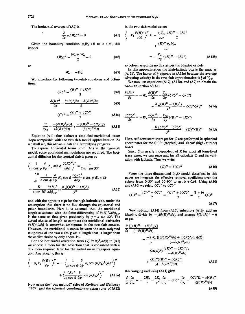
The horizontal average of (A2) is

ps(W•> • = 0 (A5) Oz

Given the boundary condition psW•--•O as z--• oo, this implies

(W•)U = W,r + W•t= 0 (A6) 2

or

W,r = - W•t (A7)

We introduce the following two-slab equations and definitions'

<R>a= <R>'* + <R>m (A8) 2

c?z 2 (A9)

<C> • <C> '*+<C> •t = (A10) 2

& -(o<R>•/Oy) -(<R> •- <R>Wy gYR- (3<R)•/&) • (3<R)a/&) (All)

Equation (All) thus defines a simplified meridional tracer slope compatible with the two-slab model approximation. As we shall see, this allows substantial simplifying progress.

To express horizontal terms from (A1) in the two-slab model, some additional manipulations are required. The horizontal diffusion for the tropical slab is given by

1 • O(R)a• '• _ 1 cos •b O•b Ky cos •b aO•b / - 2•a 2 sin 30 ø

fo ø 1 3 3(R) • acos•b0-•Kycøs•b a0•b acos•bd2ad•b K• o<R> • K,(<R> •'- <R>")

-• (A12) a tan 30 ø ag•b3oo y2

and with the opposite sign for the high-latitude slab, under the assumption that there is no flux through the equatorial and polar boundaries. Here it is assumed that the meridional length associated with the finite differencing of t•R)2t/at•3oo is the same as that given previously by y = a tan 30 ø. The actual choice of length to compute the meridional derivative 3(R)•/ac•& is somewhat ambiguous in the two-slab context. However, the meridional distance between the area-weighted midpoints of the two slabs gives a length that is larger than the earlier choice by only about 3 %.

For the horizontal advection term (V• c•(R)•/ac•qb) in (A1) we choose a form for the advection that is consistent with a

flux form required later for the global mean transport equation. Analytically, this is

--Ps Va gy / -- a cos •b g•b Ps cos •b(Va>a<R> a

+ •a cos •b •-• cos •b(Va) a (A13a)

Now using the "box method" rules of Kurihara and Holloway [1967] and the spherical coordinate-averaging rules of (A12)

in the two-slab model we get

O<R>A•tr psi/30 <R>hl-• - <R> tr -- Va aO• / • p•y 2 <R> tr Ps V3o

4- P•Y

= 2y ((R -- (R) •*) (A13b) as before, assuming no flux across the equator or pole.

In this approximation the high-latitude box is the same as (A13b). The hctor of • appears in (A13b) because the average advecting velocity in the two-slab approximation is • of V3o.

We now use equations (A12), (A13b), and (A7) to obtain the two-slab version of (A1).

0<•> '* •, 0<•> '* V•o ot - 0• • (<•>•'- <•>'•) + K•(<•> •'- <•>'*) y• - <C>'*<R> '* (A•4)

O<R> •' •<R> •' V3o

y2 -- (C)m(R) • (A15)

Here, self-consistent averages for C are performed in spherical coordinates for the 0-30 ø (tropical) and 30-90 ø (high-latitude) boxes.

Since C is nearly independent of R for most all long-lived trace gases, we can once and for all calculate C and its vari- ation with latitude. Thus we write

<C>•t = b<C> '• (A16)

From the three-dimensional N:O model described in this paper we integrate the effective removal coefficient over the sphere from 0-30 ø and 30-90 ø to get b • 0.68. Using (A10) and (A16) we relate (C) n to (C) '•

<C>U = <C> '* + <C>h* __ <C> '* + b<C> '• - (1 + b) <C>, * 2 2 2

(A17)

Now subtract (A14) from (A15), substitute (A16), add an identity, divide by -y(c•(R)a/c•z), and assume c•/c•t(R)a= 0 to get

• [(<R> •'- <R>")/y] gt

-2w,, {[(o<R>•'/&) + (o<R>"/Oz)]/2} Y

((R) •-- -- (2Ky/y 2)

<C)"(<R) '•-- b<R) m) +

y(--3<R)a/3z) (A18)

Rearranging and using (A11) gives

• c3z _ 2Wt,. 2K•, c3z (C)t • •z_ 3t 3yR y y2 3ya 3ya

<C>,r(1 - b)<R> m

(A19)

MAHLMAN ET AL.: SIMULATION OF STRATOSPHERIC N:O 2703

Now eliminate (R)'" from (A8) and (All) to obtain

(R) •'t = (R) H (A20) 2 0z

This is now in terms of globally averaged quantities. Substitute (A20) into (A19) to get

- + (A21) y (Oca)n/Oz) 2 Oya

We now set the left-hand side to zero (assuming long-term transport/chemical equilibrium), and solve for Oz/Oya to obtain

Oz (2•,/y) -- [(1 -- b)(C)"/yO In Oya OKy/y 2 + [(1 + b)/2(C)" (A22)

Before we engage in a more complete analysis, some simple physically useful insights can be gained by inspecting the character of (A22) for the "slow-chemistry limit." That is, the case in which (C)•'• O. The actual range of applicability will be assessed with the more complete solution of the problem. Near this slow chemistry limit (A22) becomes

0z - •, Upward advection velocity • • - (A23) Oye (Ky/y) Meridional diffusion velocity

Near this limit the equilibrium tracer slope must appear as a balance between the slope-steepening effect of the vertical diabatic circulation and slope-flattening effect of quasi- horizontal meridional diffusion. This result for the equilibrium tracer slope is essentially the same as that given in the companion treatment of this approach •ven by Holton [this issue]. The more general expression of (A22) differs somewhat from Holton's equation (12) mainly because of his implicit assumption that b• 1 (latitudinally invariant destruction rate).

We now assign values typical for the lower stratosphere. Assume here that the annual mean, •30 ø latitude diabatic heating rate is (Q)•'/% • 0.3 x 10 -• deg s -• and that O(T)•'/Oz << W%. (This diabatic heating rate is consistent with those obtained from the annual averages of both the GFDL "Zodiac" and "SKYHI" general circulation models at an altitude near 20 km.) This •ves from the thermodynamic equation

(Q)"/cv -• (A24) •, • • +0.03 • s (•0.8 km month -•) •/%

The observed hemispheric mean slope of quasi-conservative tracers in the stratosphere is about -1 x 10 -• [Machta and Tele•adas, 1973]. Using all of these numbers, we solve for K• in (A23) to get

K• • 1.1 x 10 lø cm 2 s -• (A25) This is a value which is reasonably consistent with independent estimates from a number of empirical two-dimensional transport models. However, this value of K• and the balance of (A23) are in sharp contrast to several recent two- dimensional model formulations which have argued that meridional diffusion is of secondary importance [Holton, 1981; Garcia and Soloman, 1983; Tun•, 1984] provided that a "proper" meridional circulation is used (e.g., Lagrangian mean, diabatic, or "residual"). It is also interesting to note that this inferred K• value of 1.1 x 10 •ø cm 2 s -• is in the range

identified in the theoretical/modeling study of R. A. Plumb and J. D. Mahlman (unpublished manuscript, 1986). They find an effective Ky value of about 2 x 10 •ø crn 2 s-• in the subtropical anticyclone "surf zone" area and about 0.3 x 10 •ø cm '• s-• in mid-latitudes. We note that these values may not be strictly comparable, since the two-slab value of Ky is essentially appropriate for flux across the 30 ø latitude circle. This is near the poleward edge of the subtropical "surf zone" identified by R. A. Plumb and J. D. Mahlman (unpublished manuscript, 1986).

A recent study by Ko et al. [1985] on two-dimensional transport modeling in isentropic coordinates suggests a K• value of about 0.3 x 10 •ø cm 2 s-•. This is more than a factor

of 3 lower than that suggested by the above analysis. The explanation for this discrepancy may be due to the local "surf zone" effect mentioned above, the crudity of the two-slab model, or possibly, other factors.

With these preliminary insights gained we now proceed to complete the analysis begun through the derivation of (A22). If the original assertion of section 3 is indeed correct, (A22) can be evaluated directly. That is because the indication was that globally averaged one-dimensional behavior is directly predictable for suitably long-lived, fully equilibrated trace gases (exceptions arising upon violation of these two requirements are given by Mahlman [1975]). This assertion implies that the only R dependence in (A22) (0 In (R)"/Oz) can be solved independently of (A22). We now investigate the global properties of the two-slab model to evaluate that assertion.

To produce a fully self-consistent global mean equation, we first combine the mass continuity equation (A2) in log pressure coordinates with (A1) to obtain the flux form tracer continuity equation in the two-slab model (see equation (A13)).

p$ • •

p$ • •

0(e)"_ _ __0 p,W,,(e)" p,V•o ((e?'+ Ot Oz 2y

+ (K/y2X(•) n'- (e)")- (c)"(l•)" (A26)

O(R) h' t9 psV3o ((R)h, + (R)") Ot - + • psW•'(R)*' + 2y -- (K•,/y2)((R) •a -- (R)"') -- b(C)"'(R) •a (A27)

Here, we have used equations (A7), (A12), and (A16). Now we average (A26) and (A27) to obtain the global average equation

0 ((R)" + (R) •a)

--• ((R)" + b(R) •') (A28)

Next, introduce equation (All) and assume O(R)n/Ot = 0 to obtain

O y tgz tg(R) H O= - •zzpSW,, 2 OyR Oz

2 (1 + b)(R)ht + y 0y• • -] (A29) We then eliminate (R) *t, using (A20) to get after some ma-

nipulation

o=-• p,W,, 5 o•

[(1 + b) --(C)" p$ 2 (R)n + (1 - b)

4 Y ay R •ZZ '3 (A30)

2704 MAHLMAN ET AL.' SIMULATION OF STRATOSPHERIC N20

Note that the form of equation (A30) is equivalent to the global average eddy diffusion equation for equilibrium (in log pressure coordinates)

r3 r3 ( R ) n •-• Ps K: &z ps(CR)"= 0 (A31)

where from (A30), Kz is defined in the two-slab model by

Y W,r &z (A32) i%(R) _= - Near the "slow-chemistry" limit we get from (A23) and (A32) that Kz • y2 Wtr2/2Ky. This is very close to the value obtained by Holton's companion analysis [Holton, this issue, equation (14)3.

With this we are now in a position to gather a number of insights about the chemistry/transport problem under consideration here. First and easiest, note that the global chemical destruction term in (A30) is already considerably more complex than that traditionally used in one-dimensional models. This is because both C and R vary with latitude. Thus (CR) n depends in (A30) upon &/•YI• as well as upon global mean and precomputed quantities (such as b). Further, recall that c3z/c3y R in (A22) can change depending upon the size of the chemical destruction (C) t•. It is of interest to note that the chemistry term in A30 provides a straightforward approach to parameterization of nonlinear chemical effects in a one- dimensional model.

Most significantly for the present development, (A32) shows that the global one-dimensional diffusion coefficient can change with different trace constituents. This is because c3z/c3yl• in (A22) depends upon the efficiency of the chemical destruction. We have yet to determine, however, the relative importance of this effect.

Another useful insight provided by (A32) is a straightforward explanation of the empirical observation that K• increases with altitude in the upper stratosphere. As stated earlier, W,• depends upon the dynamical forcing of the stratosphere away from a radiative equilibrium state. Because this departure increases notably with altitude, K• must also do so.

The most important insight to be gained from this analysis is that in general a complete solution of the meridional tracer slope structure and the global mean vertical structure depends upon a mutually consistent solution of equations (A22) and (A30). Thus r3z/r3y• in (A22) depends upon (R) n, while (R) n in (A30) depends upon r3z/r3ya. Note that this, in principle, refutes both provisional assertions in section 3:(1) that once (R) n is determined for a given tracer with an appropriately determined K: profile, that profile will work for other long- lived constituents, and (2) all long-lived trace constituents exhibit the same meridional slopes.

We now discuss the methods one might utilize to solve equations (A22) and (A30) for 3z/r3ya and (R) n. The most straightforward, of course, is simply to substitute for 3z/3ya in (A30), using (A22). This operation yields a linear second-order differential equation in (R) n with complicated and variable coefficients. Solving this combined equation for (R) n in turn allows direct determination of r3z/r3yl• from (A22).

Because of the direct physical significance of equations (A22) and (A30), greater insight into the relationship between them can be gained by solving them iteratively. A reasonable way to begin is to assume that (C) t'--•0 initially, so that r3z/r3ya(0) is given by (A23). This value is then substituted into (A30), and (A30) is solved for (R)n(z). From this r3 In (R)n/3z (1) is substituted back into (A22) to get r3z/r3ya(1) and so on.

Since here we are only interested in the degree of coupling between (A22) and (A30), for clarity we seek to simplify the problem. A simple analysis of the square-bracketed term in (A30) shows that the scale height of (R) n has to be smaller than 1.8 km before the second term is within 20% of the magnitude of the first term. Later results indicate that such small-scale heights (large gradients) are to be expected only for extremely rapid removal chemistries. At that limit this simple model becomes inappropriate anyway. Thus we neglect the second term within the square brackets of (A30) to give to an excellent approximation

r3 r3(R) n (1 + b) (R)n • 0 (A33) ps(-e ) - ps < C ) '" 2' where K•(R) is given by (A32).

Now for analytical convenience we assume that psKz(R) constant with height and also that ps(C) • (1 + b/2) • constant with height. From the lower to the upper stratosphere these are not bad approximations, at least for the present purpose. Under these restrictive assumptions, (A33) has the analytic solution

(R)U(z) (R) u exp- [(1 + b) (C)t'] - z' (A34)

where z'= z- %op, and Zt•op is some "tropopause" height below which (R) a is assumed well mixed and constant. Under these simple conditions, (A34) gives us

O In (R) n [!1 + b) Oz = - 2 K'-•] (A35) Substituting (A35) into (A22) yields

Oy • -W,. + K:X/2(C)'"x/2(1/2 -- b/2) x/2 (A36) Oya (K•,/y) + y(C)"'(1/2 + b/2)

We recall here that K: is dependent upon Oz/Oya, as shown in (A32). The convenient simplification leading to (A34) and (A35) now allows us to evaluate the effect of chemical destruction on the flattening of meridional tracer slopes, with and without "K• feedback." Here, "K• feedback" simply means that K• depends upon Oz/OyR and that a fully self-consistent calculation must take that into account. However, to clarify the importance of this effect, we solve (A36) in two ways, with and without "K• feedback."

For the no K• feedback case, we set Kz at its "slow- chemistry" limit from (A32), using previously obtained values

- 3.6783 x • 10 • cm -2

K• (slow chem) • 2 x 0.03 cm s ,.

x(-1 x 10 -3 )•5.5 x 103cm

This value is close to those used for the region near 20 km in carefully calibrated one-dimensional models [e.g., McElroy et al., 1974' Hunten, 1975]. We now use this value for K• to solve (A36) for a wide range in values for (C)tL For convenience the other values previously established are' W•,- 0.03 cm K• = 1.1 x 10 TM cm 2 s-X'y- 3.6783 x 108 cm, and b = 0.68. The slope values obtained are given in the thin-dashed "no K: feedback" curve in Figure A1. Figure A1 shows that the predicted slope is within 85% of the maximum value (-1 x 10 -3) for local photodestruction times (1/(C) •') exceeding • 1000 days. However, for 1/(C)"'• 100 days, the predicted slope is only about 42% of the "slow-chemistry" value. Thus for chemical destructions of intermediate time scale we already expect a noticeable flattening of the equilibrium slopes. A

MAHLMAN ET AL.' SIMULATION OF STRATOSPHERIC N20 2705

lxlO -6 -.lx10 -3 -.2

EQUILIBRIUM TRACE CONSTITUENT SLOPE ( a z -.3 -.4 -.5x10 -3 -.6 -.7

I I I I I -.8 -.9 -1.x10 -3

11.6

c3Z

-•YYR with "K z Feedback"

8Z

c3 yR with o "K Z Feedback"

lx10 I I I :1 0 -20% -40% -60% -80% -100%

- 23.1

- 579

- 116

- 232.

579

1158

2315

5787

11574.

% OF Kz FOR INERT TRACER

Fig. Ai. Two-slab model predictions for effect of chemical destruction on global one-dimensional Kzs and meridional trace constituent slopes. The ordinate is (C) tr, the "tropical" mean photodestruction coefficient. The lower abscissa is the percentage reduction of Kz from its "slow-chemistry" limit. The upper abscissa is the equilibrium meridional trace constituent slope.

schematic diagram of these slope-affecting processes is given in Figure A2.

The flattening of these predicted slopes for reasonable chemical destruction time scales implies that K• (from A32) should also be importantly effected. We next introduce the effect of "K• feedback" by substituting (A32) into (A36) and writing the result in the form

-W,, + (-?z/?yR)•/2{,(c},,'/2EyW,/(1 + b)(1/2 - b/2) (K/y) + y< C)"(1/2 + b/2)

(A37)

where the n enclosed in superscript braces represents an iter- ation index. Note that (A37) is formally quadratic in •z/•y, and thus could be solved directly. Here, however, we choose to solve (A37) in the indicated iterative manner to maximize our understanding of the effect of "Kz feedback" on the meridional isoline slopes. This procedure demonstrates that the convergence to the proper solution is very rapid in (A37), typically requiring three or fewer iterations to converge to four-place accuracy. The results for this calculation are given by the heavy solid line in Figure A1. Notice in Figure A1 that the predicted meridional s!opes are very similar to that obtained in the "no K• feedback" limit of (A36).

Thus the meridional slopes of tracer isolines are very depe-

nent upon the chemical destruction rate, but the relative effect of "K• feedback" is small except for very fast destruction chemistries. However, the effect of the more complete calculation is to moderate somewhat the slope-flattening effect of the destruction chemistry.

In the companion analysis of Holton [this issue] the second term in the numerator of (A36 or A37) does not appear, by virtue of his assumption that b • 1. Analysis of the complete solution of (A37) suggests that his simplification of our analysis is indeed reasonable. The largest values of this term occur at high-destruction rates ((C) t• = 10 -6 s-•), where it becomes about 12% of W•,. At (C) '• = 10 -8 s -• the term has about a 4% effectß Thus at this level of approximation the 3z/3y• equation (A37) is effectively decoupled from the K• equation (A32). Remember, however, that the Kz value is strongly affected by the slope-flattening effect of chemical destruction, as determined by (A37).

The lower scale in Figure A1 shows the dependence of K• in this two-slab model on the value of the photodestruction coefficient (C) '• (expressed as a percentage of the K• appropriate for a nearly inert tracer). This shows that the effective K• in this model becomes much smaller in regions where (C) '• becomes quite large. In this context then, one-dimensional models using a fixed K• might calculate too much vertical transport of substances in regions characterized by rapid destruction rates. It would be of interest to evaluate this effect in a comprehensive one-dimensional photochemical model to see


30

20

10

Diffusion

Mixing Ratio Isolines

Pole Equator LATITUDE

EQUILIBRIUM SLOPE MECHANISMS

Fig. A2. Schematic diagram illustrating the three competing processes determining the equilibrium meridional slopes of trace constituent isolines: the slope-steepening effect of the diabatic circulation, and the slope-flattening effects of irreversible meridional diffusion and photochemical destruction.

the model sensitivity to this type of change. This could be readily tested in a one-dimensional model through an iterative coupling of equations (A22) and (A30).

The physical interpretation of this reduced K: effect is quite straightforward. In the two-slab model, the net vertical flux depends upon (for an "upward" tracer) the tracer amount moving upward in the tropical box being larger than the amount moving downward in the high-latitude box. A reduced slope for a given global mean vertical gradient means a reduced value of meridional gradient ((R} tr- (R} ht) (see equation (A28)). It should be noted that this effect could be less in the real atmosphere as a result of the additional presence of local vertical transport events that are somewhat diffusive in character, in contrast to the advective character of the global mean vertical flux in the two-slab model.

Acknowledgments. The authors are grateful to J. Bacmeister, J. R. Holton, R. A. Plumb, J. Sarmiento and an anonymous reviewer for their perceptive comments and suggestions on the work presented here. J. Kennedy, J. Connor, and P. Tunison's group provided valu- able technical assistance.

REFERENCES

Ackerman, M., Ultraviolet solar radiation related to mesospheric processes, in Mesospheric Models and Related Experiments, pp. 149- 159, D. Reidel, Hingham, Mass., 1971.

Andrews, D. G., and M. E. Mcintyre, Planetary waves in horizontal and vertical shear: The generalized Eliassen-Palm relation and the mean zonal acceleration, J. Atmos. Sci., 33, 2031-2048, 1976.

Andrews, D. G., J. D. Mahlman, and R. W. Sinclair, Eliassen-Palm diagnostics of wave, mean-flow interaction in the GFDL "SKYHI" general circulation model, J. Atmos. Sci., 40, 2768-2784, 1983.

Breiland, J. G., Comparison of the vertical distribution of thermal stability in the lower stratosphere with the vertical distribution of ozone, J. Atmos. Sci., 24, 569-576, 1967.

Breiland, J. G., Some large-scale features of the vertical distribution of atmospheric ozone associated with the thermal structure of the atmosphere, J. Geophys. Res., 73, 5021-5028, 1968.

Dobson, G. M. B., The laminated structure of ozone in the atmosphere, Q. J. R. Meteorol. Soc., 99, 599-607, 1973.

Dickinson, R. E., Theory of planetary wave-zonal flow interaction, J. Atmos. Sci., 26, 73-81, 1969.

Dunkerton, T., On the mean meridional mass motions of the stratosphere and mesosphere, J. Atmos. Sci., 35, 2325-2333, 1978.

Ehhalt, D. H., E. P. Roth, and U. Schmidt, On the temporal variance of stratospheric trace gas concentrations, J. Atmos. Chem., 1, 27-51, 1983.

MAHLMAN ET AL.: SIMULATION OF STRATOSPHERIC N20 2707

Fels, S. B., J. D. Mahlman, M.D. Schwarzkopf, and R. W. Sinclair, Stratospheric sensitivity to perturbations in ozone and carbon dioxide: Radiative and dynamical response, J. Atmos. $ci., 37, 2265-2297, 1980.

Frederick, J. E. and J. E. Mentall, Solar irradiance in the stratosphere: Implications for the Herzberg continuum absorption of 02, Geophys. Res. Lett., 9, 461-464, 1982.

Garcia, R. R., and S. Soloman, A numerical model of the zonally averaged dynamical and chemical structure of the middle atmosphere, J. Geophys. Res., 88, 1379-1400, 1983.

Goldan, P. D., W. C. Kuster, D. L. Albritton, and A. L. Schmeltekopf, Stratospheric CFC13, CF212, and N20 height profile measurements at several latitudes, J. Geophys. Res., 86, 413-423, 1980.

Hampson, R. F. (Ed.), Chemical kinetic and photochemical data sheets for atmospheric reactions, FAA Rep. FAA-EE-80-17, 490 pp., Fed. Aviat. Admin., Washington, D.C., 1980.

Hess, P. G., and J. R. Holton, The origin of temporal variance in long-lived trace constituents in the summer stratosphere, J. Atmos. $ci., 42, 1455-1463, 1985.

Holton, J. R., Wave propagation and transport in the middle atmosphere, Philos. Trans. R. $oc. London, $er. A, 296, 73-85, 1980.

Holton, J. R., An advective model for two-dimensional transport of stratospheric trace species, J. Geophys. Res., 86, 11,989-11,994, 1981.

Holton, J. R., A dynamically based transport parameterization for one-dimensional photochemical models of the stratosphere, J. Geo- phys. Res., this issue.

Hunten, D. M., The philosophy of one-dimensional modeling, Pro- ceedings of the Fourth Conference on the Climatic Impact Assess- ment Program, Rep. DOT-TSC-OST-75-38, pp. 147-155, U.S. Dep. of Transp., Washington, D.C., 1975.

Jones, R., and J. Pyle, Observations of CH 4 and N20 by the Nimbus 7 SAMS: A comparison with in situ data and two dimensional model calculations, J. Geophys. Res., 89, 5263-5279, 1984.

Junge, C. E., Residence time and variability of tropospheric trace gases, Tellus, 26, 477-488, 1974.

Ko, M. K. W., K. K. Tung, D. K. Weisenstein, and N. D. Sze, A zonal-mean model of stratospheric tracer transport in isentropic coordinates: Numerical simulations for nitrous oxide and nitric

acid, J. Geophys. Res., 90, 2313-2329, 1985. Kurihara, Y., and J. L. Holloway, Jr., Numerical integration of a

nine-level global primitive equations model formulated by the box method, Mon. Weather Rev., 95, 509-530, 1967.

Levy, H., II, and J. D. Mahlman, Modeling tropospheric N20, in Proceedings of the NA TO Advanced Study Institute on Atmospheric Ozone: Its Variations and Human Influences, edited by A. C. Aikin, pp. 893-907, Federal Aviation Administration, Washington, D.C., 1980.

Levy, H., II, J. D. Mahlman, and W. J. Moxim, A preliminary report on the numerical simulation of the three-dimensional structure and

variability of atmospheric N20, Geophys. Res. Lett., 6, 155-158, 1979.

Levy, H., II, J. D. Mahlman, and W. J. Moxim, Tropospheric N20 variability, $. Geophys. Res., 87, 3061-3080, 1982.

Levy, H., II, J. D. Mahlman, and W. J. Moxim, Tropospheric ozone: The role of transport, J. Geophys. Res., 90, 3753-3772, 1985.

Machta, L., and K. Telegadas, Examples of stratospheric transport, Proceedings of the Second Conference on the Climatic Assessment Program, Rep. DOT-T$C-OST-73-4, pp. 47-56, U.S. Dep. of Transp., Washington, D.C., 1973.

Mahlman, J. D., Some fundamental limitations of simplified transport

models as implied by results from a three-dimensional general- circulation tracer model, Proceedings of the Fourth Conference on the Climatic Impact Assessment Program, Rep. DOT-TSC-OST- 75-38, pp. 132-146, U.S. Dep. of Transp., Washington, D.C., 1975.

Mahlman, J. D., Mechanistic interpretation of stratospheric tracer transport, Issues in Atmospheric and Oceanic Modeling, Advances in Geophysics, vol. 28A, Climate Dynamics, edited by B. Saltzman, pp. 301-320, Academic, Orlando, Fla., 1985.

Mahlman, J. D., and W. J. Moxim, Tracer simulation using a global general circulation model: Results from a mid-latitude instantaneous source experiment, $. Atmos. Sci., 35, 1340-1374, 1978.

Mahlman, J. D., and L. J. Umscheid, Dynamics of the middle atmosphere: Successes and Problems of the GFDL "SKYHI" general circulation model, in Dynamics of the Middle Atmosphere, edited by J. R. Holton and T. Matsuno, pp. 501-525, Terra Scientific, Tokyo, 1984.

Mahlman, J. D., H. Levy II, and W. J. Moxim, Three-dimensional tracer structure and behavior as simulated in two ozone-precursor experiments, J. Atmos. Sci., 37, 655-685, 1980.

Mahlman, J. D., D. G. Andrews, D. L. Hartmann, T. Matsuno, and R. G. Murgatroyd, Transport of trace constituents in the stratosphere, Dynamics of the Middle Atmosphere, edited by J. R. Holton and T. Matsuno, pp. 387-416, Terra Scientific, Tokyo, 1984.

Manabe, S., and J. D. Mahlman, Simulation of seasonal and interhemispheric variations in the stratospheric circulation, J. Atmos. Sci., 33, 2185-2217, 1976.

McElroy, M. B., Sources and sinks for nitrous oxide, in Proceedings of the NATO Advanced Study Institute on Atmospheric Ozone: Its Variations and Human Influences, edited by A. C. Aikin, p. 345-364, Federal Aviation Administration, Washington, D.C., 1980.

McElroy, M. B., S. Wofsy, J. Penner, and J. McConnell, Atmospheric ozone: Possible impact of stratospheric aviation, J. Atmos. Sci., 31, 287-303, 1974.

Moortgat, G. K., and E. Kudszus, Mathematical expression for the O('D) quantum yields from the 0 3 photolysis as a function of temperature (230-320øK) and wavelength (295-320 nm), Geophys. Res. Lett., 5, 191-194, 1978.

Plumb, R. A., Eddy fluxes of conservative quantities by small- amplitude waves, J. Atmos. Sci., 36, 1699-1704, 1979.

Schemltekopf, A. L., et al., Stratospheric nitrous oxide profiles at various latitudes, $. Atmos. Sci., 34, 729-736, 1977.

Selwyn, G., J. Podolske, and H. S. Johnston, Nitrous oxide ultraviolet absorption spectrum at stratospheric temperatures, Geophys. Res. Lett., 4, 427-430, 1977.

Simon, P., Irradiation solar flux measurements between 120 and 400 nm: Current position and future needs, Planet. Space Sci., 26, 355- 365, 1978.

Tung, K. K., Modeling of tracer transport in the middle atmosphere, Dynamics of the Middle Atmosphere, edited by J. R. Holton and T. Matsuno, pp. 417-444, Terra Scientific, Tokyo, 1984.

Wofsy, S.C., Interactions of CH4 and CO in the earth's atmosphere, Annu. Rev. Earth Planet. Sci., 4, 441-469, 1976.

H. Levy II, J. D. Mahlman, and W. J. Moxim, Geophysical Fluid Dynamics Laboratory, Princeton University, P.O. Box 308, Prince- ton, NJ 08542.

(Received April 22, 1985; revised November 19, 1985;

accepted November 22, 1985.)

three-dimensional simulations of stratospheric no' - … · 2016-05-09 · three-dimensional...

Documents