three-dimensional ocean sensor networks: a survey · ocean sensor network (osn), formed by...

J. Ocean Univ. China (Oceanic and Coastal Sea Research) Review DOI 10.1007/s11802-012-2111-7 ISSN 1672-5182, 2012 11 (4): 436-450 http://www.ouc.edu.cn/xbywb/ E-mail:[email protected]

Three-Dimensional Ocean Sensor Networks: A Survey

WANG Yu1), *, LIU Yingjian2), 1), and GUO Zhongwen2)

1) Department of Computer Science, University of North Carolina at Charlotte, Charlotte, North Carolina 28223, USA

2) Department of Computer Science and Technology, Ocean University of China, Qingdao 266100, P. R. China

(Received July 17, 2012; revised September 3, 2012; accepted September 25, 2012) © Ocean University of China, Science Press and Springer-Verlag Berlin Heidelberg 2012

Abstract The past decade has seen a growing interest in ocean sensor networks because of their wide applications in marine re-search, oceanography, ocean monitoring, offshore exploration, and defense or homeland security. Ocean sensor networks are gener-ally formed with various ocean sensors, autonomous underwater vehicles, surface stations, and research vessels. To make ocean sen-sor network applications viable, efficient communication among all devices and components is crucial. Due to the unique character-istics of underwater acoustic channels and the complex deployment environment in three dimensional (3D) ocean spaces, new effi-cient and reliable communication and networking protocols are needed in design of ocean sensor networks. In this paper, we aim to provide an overview of the most recent advances in network design principles for 3D ocean sensor networks, with focuses on de-ployment, localization, topology design, and position-based routing in 3D ocean spaces.

Key words ocean sensor networks; underwater sensor networks; three-dimensional sensor networks; ocean applications; 3D de-ployment; topology design; localization; position-based routing

1 Introduction

Nearly 71% of the Earth’s surface is covered by water. The deep ocean is a vast and mostly unexplored habitat on our planet. Recently, there has been a growing interest in exploring and monitoring ocean environments for scien-tific exploration, commercial exploitation, or defense and security purposes. Ocean sensor network (OSN), formed by underwater networks of distributed sensors, is an ideal system for this type of extensive monitoring and explora-tion tasks.

Ocean sensor network is a type of underwater wireless sensor network (UWSN) (Akyildiz et al., 2005; Cui et al., 2006; Akyildiz et al., 2007; Heidemann et al., 2012), which is generally formed by various ocean sensors, sta-tionary moorings, autonomous underwater vehicles, sur-face research vessels, or even coastal radars and large gliders. Different types of underwater devices in an OSN can communicate with each other via underwater com-munication techniques to form an underwater wireless network, while different types of ocean sensors can per-form various sensing and monitoring tasks for marine applications. With the great potential to enable a wide range of applications and enhance the ability to observe and predict the ocean environments, ocean sensor network has recently become an extremely hot research area around the world.

* Corresponding author. E-mail: [email protected]

However, due to the unique characteristics of under-water communication channels (Sozer et al., 2000; Chitre et al., 2008), such as low communication bandwidth, se-vere fading and multipath effects, large propagation delay, and high error rate, efficient and reliable underwater communication in ocean sensor networks is very chal-lenging and significantly different from the one for ter-restrial wireless sensor networks. The typical underwater communication is based on acoustic wireless communica-tion (Sozer et al., 2000; Chitre et al., 2008). Underwater communication was first used in the military such as in the submarine communication system developed in the United States around the end of the Second World War. With continued research over these years, different new physical layer or link layer techniques (such as modulation, coding, multiple access, media access, error detection and recov-ery) have been developed to improve the performance of acoustic communication in salty ocean water. For more details on these techniques, please refer to survey papers by Sozer et al. (2000), Akyildiz et al. (2007), Chitre et al. (2008) and, Heidemann et al. (2012). In this paper, we instead focus on recent advances of network design prin-ciples (such as deployment, localization, topology control, and routing) for ocean sensor networks.

Notice that most existing wireless sensor network sys-tems and protocols are based on two-dimensional (2D) design, where all sensor nodes are distributed in a two dimensional plane. This assumption is justified for appli-cations where sensor nodes are deployed on earth surface and where the height of the network is smaller than

WANG et al. / J. Ocean Univ. China (Oceanic and Coastal Sea Research) 2012 11 (4): 436-450

437

transmission radius of a node. However, this 2D assump-tion may no longer be valid in ocean sensor networks, where sensors are distributed over a three-dimensional (3D) space and the difference in the third dimension (depth) is too large to be ignored. Sensor network prob-lems in 3D have not been adequately analyzed until re-cent. Unfortunately, the design of 3D networks is surpris-ingly more difficult than the design in 2D (Wang, 2013). Many properties of the 3D network require additional computational complexity, and many problems cannot be solved by extensions or generalizations of 2D methods. In facing up to these challenges, there have been new net-work protocols and algorithms specifically designed for 3D sensor networks by exploring rich geometric proper-ties of 3D sensor networks. In this paper, we aim to pro-vide an overview of the most recent advances in network design principles for 3D ocean sensor networks, with focuses on deployment, localization, topology design, and position-based routing in 3D ocean spaces.

The remainder of this paper is organized as follows. In Section 2, we introduce some examples of current appli-cations or systems of ocean sensor networks. In Sections 3, 4, 5 and 6, we discuss 3D deployment, localization, topology design, and position-based routing for 3D ocean sensor networks in detail, respectively. Finally, we con-clude the paper in Section 7.

2 Ocean Sensor Network Applications

Applications of ocean sensor networks include oceano-graphic data collection, scientific ocean sampling, pollu-tion and environmental monitoring, ocean climate re-cording, marine commercial operations, offshore oil ex-ploration, disaster prevention, assisted navigation, dis-tributed surveillance, etc. These applications can be roughly categorized into three classes: scientific applica-tions, industrial applications, and defense applications (Heidemann et al., 2012). Since many new applications are emerging, it is infeasible to give an exhaustive list of ocean sensor network applications. Next, we briefly re-view some representative examples in each class.

2.1 Scientific Applications

Scientific applications of ocean sensor networks mainly serve to observe the ocean environment for various scien-tific research purposes. Possible sensing objectives of ocean sensor networks include geological processes on the ocean floor, ocean water characteristics (temperature, salinity, oxygen levels, bacterial and other pollutant con-tent, etc.), activities of marine animals (microorganisms, fish, or mammals). Next, we describe two example sys-tems of ocean sensor networks in scientific applications.

Autonomous Ocean Sampling Network (AOSN): Ocean phenomena such as fronts, wind-driven red tides and mixing upwelling are rapidly changing dynamic proc-esses with highly spatial and temporal characteristics. With the regular static mooring sensing system, it is dif-ficult to observe these dynamic ocean phenomena (Zhang

et al., 2012). Curtin et al. (1993) proposed the AOSN concept which leverages autonomous mobile platforms to observe dynamic ocean fields. Sampling of the high gra-dients associated with the front is done with several autonomous underwater vehicles (AUVs) as well as with distributed acoustic and point sensors. The vehicles trav-erse the network recording temperature, salinity, current velocity, and other items, relaying key observations to the network nodes in real time and transferring more com-plete data sets after docking at a node. Each network node consists of a base buoy or mooring containing an acoustic beacon, an acoustic modem, point sensors, an energy source and a selectable number of AUV docks. Acoustic transmission loss along the many inter-nodal paths is measured periodically. A central location, either one of the nodes and/or onshore, processes the information in nearly real time to guide vehicle sampling. One of the major milestones for AOSN is the automated control of multiple, mobile sensors for weeks using spatial coverage metrics (Curtin and Bellingham, 2009). Control of an array of platforms (gliders) constrained to a fixed sam-pling pattern for a month has been demonstrated with no person in the loop (Paley et al., 2008).

Coastal Ocean Monitoring and Prediction System (COMPS): The COMPS (Weisberg et al., 2009) is a con-tributor toward an emergent Regional Coastal Ocean Ob-serving System for the southeastern United States. The system is intended to provide a supportive framework for red-tide prediction as well as for other coastal ocean mat-ters of societal concern. The coastal ocean element of COMPS is comprised of: 1) buoys with acoustic Doppler current profilers for full water column currents, tempera-ture and salinity sensors at a few discrete depths, and sur-face meteorological sensors; 2) high frequency radar for surface current mapping; 3) bottom stationed ocean pro-filers (BSOP) for discrete profiles of temperature and salinity; and 4) various data analysis products. A total of six buoys with real-time telemetry are presently main-tained, five with surface meteorological measurements in addition to in-water sensors. In addition to these surface moorings with telemetry four other (subsurface) moorings are also maintained. The subsurface wave sensors are linked by acoustic modems to either a surface buoy or a fixed tower at two experimental near shore sites. COMPS is also planning to deploy BSOP in conjunction with gliders. By combining the attributes of BSOP (synoptic sampling at high vertical resolution, but limited horizon-tal resolution) with those of gliders (high spatial resolu-tion, but non-synoptic sampling), the intention is to pro-vide three dimensional maps of temperature, salinity and other data fields for description and assimilation into models.

2.2 Industrial Applications

Industrial applications of ocean sensor networks are mainly associated with monitoring and controlling un-derwater commercial activities, such as installation of underwater equipment related to oil or mineral extraction,


438

underwater pipelines, or commercial fisheries. Different from scientific applications, industrial applications usu-ally involve control and actuation components (Heide-mann et al., 2012). Here, we just review an example sys-tem used for pipeline monitoring.

With the increasing demand for energy and water in the world, petroleum, natural gas, and water resources and facilities have become important assets for most countries. One of the major facilities for using these resources is pipelines and a large portion of these pipelines are de-ployed under ocean water. Two types of threats may occur in pipeline-laying infrastructures: intentional and non-

intentional (Mohamed et al., 2011). Intentional threats include terrorist attacks or illegal tapping. Non-intentional threats may occur due to accidents such as ships crashing onto a pipeline, human mistakes in the pipeline operation or maintenance, or natural disasters such as those associ-ated volcanoes and earthquakes. Therefore, it is crucial to keep monitoring the health of every underwater pipeline and preventing or detecting any possible threat. Manum and Schmid (2007) reported an acoustic ocean sensor network used for monitoring vibrations in the Langeled Pipeline installed at a depth of 800–1100 meters on a hilly and rocky seabed. Several segments of the pipeline are not in contact with the seabed. With strong sea currents, high vibrations may be induced in these free segments. This introduces high and risky pressure on the pipeline segments. The monitoring network consists of autono-mous synchronized wireless acoustic nodes. These nodes use acoustic Clamp Sensor Packages (CSP) mounted on the pipeline at regular intervals and Master Sensor Pack-ages (MSP) for monitoring the vibrations in longer pipe-line free segments. The CSPs are equipped with batteries that last for six months. Remote operating vehicles are used to replace dead nodes.

2.3 Defense Applications

Defense applications of ocean sensor networks include safeguarding or monitoring port facilities or ships in har-bors, detecting and removing sea mines, providing com-munication with submarines and divers, and assisting navigation of battle ships or submarines in enemy’s sea areas.

Detecting, classifying, and tracking underwater targets are indispensable components of modern underwater de-fense systems. Using traditional sonar arrays may be dif-ficult and impractical in some mission-critical scenarios, because they should be mounted on or towed by a ship or a submersible. Alternatively, acoustic ocean sensor net-works offer a promising approach (Isbitiren and Akan, 2011). Cayirci et al. (2006) introduced a classification-

mining-based detection and classification scheme for tac-tical ocean sensor networks, in which mechanical, radia-tion, magnetic and acoustic micro-sensors are used. Their scheme first detects a target in the vicinity based on the readings of radiation and mechanical sensors. Then the detected target is classified into one of the following tar-get types based on the data coming from acoustic and magnetic micro-sensors: a diver, a SEAL delivery vehicle, a submarine or a mine. Barr et al. (2011) presented the first set of results for constructing a barrier to detect in-truding submarines in a 3D sensor network where sensor nodes are distributed randomly and uniformly. Their de-ployment method guarantees to create a vertical barrier without any hole.

Seaweb (Rice, 2007) is an example of a large-scale ocean sensor network used for defense, which is being developed by the US Navy since the 1980s. It employs AUVs, gliders, buoys, repeaters and ships where the component devices communicate via telesonar, radio or satellite links (see Fig.1 for an illustration). Telesonar

Fig.1 Seaweb network in the Eastern Gulf of Mexico, including three AUVs, six repeater nodes, and two gateway buoys (Rice, 2007).


439

links enable underwater communication, radio links are used only by the devices on the surface to communicate with the command center on the ship, and the on-shore command center is accessed via satellite links.

3 3D Deployment of Ocean Sensor Networks

Ocean sensor networks are usually deployed in 3D un-derwater spaces, except for a few sensor networks de-ployed only on the surface (Guo et al., 2008) or at the bottom (Akyildiz et al., 2007) of the ocean. Due to the wide range of applications of ocean sensor networks, there are different ways to deploy underwater sensors in ocean environment. Based on the mobility of nodes, we can roughly categorize them into three groups: static de-ployment, semi-mobile deployment, and mobile deploy-ment. We will review several different 3D deployment methods of ocean sensor network in this section.

Besides mobility, other important parameters that char-acterize a deployment include network density, coverage, and number of nodes. Compared to those for terrestrial sensor networks, underwater deployments are generally less dense, of longer range, and with significantly fewer nodes. However, it is also envisioned that a large scale of 3D ocean sensor network can become a reality in near future and be useful for more complex tasks and applica-tions.

3.1 Static Deployment

In the 3D ocean environment, ocean sensors can float at different depths to observe a given phenomenon. One possible deployment method (Cayirci et al., 2006) is to attach each ocean sensor to a surface buoy and control the length of the wire to adjust the depth of each sensor. This solution enables an easy and quick deployment of a 3D sensor network, but also suffers from certain weaknesses; for instance, multiple floating buoys may obstruct ships navigating on the sea surface or they can be easily de-tected and deactivated by enemies in military settings. Furthermore, floating buoys are vulnerable to weather and tampering or pilfering (Pompili et al., 2009). Akyildiz et al. (2005) proposed another solution that sensors can be anchored to the seafloor and equipped with a floating buoy that can be inflated by a pump. The buoy pulls the sensor towards the ocean surface. The depth of the sensor can then be regulated by adjusting the length of the wire that connects the sensor to the anchor, by means of an electronically controlled engine that resides on the sensor. In both of these solutions, ocean sensors are static after the initial deployment.

3.2 Semi-Mobile Deployment with Depth Adjustment

If the sensor nodes have the ability to adjust their posi-tions underwater, it will be easier for water column pro-filing and 3D network deployment. Although the mobility of ocean sensors is limited with the current technology, some devices have been constructed to implement depth

adjustment. For example, Howe and McGinnis (2004) developed a water column profiler which travels along the mooring cable of their system and is able to be re-charged inductively on the surface platform. The LEO-15 platform developed jointly by WHOI and Rutgers Uni-versity has a bottom-mounted winch system for water column profiling (Glenn et al., 2006). Detweiler et al. (2012) developed a depth adjustment system that is a winch-based module and can be incorporated into the core AquaNode system to enable depth adjustment in water of up to 50 m deep. The depth adjustment system enables the ocean sensors to be deployed with a desired geometry which can improve sensing and communication over the whole region. Moreover, this system makes localization and recovery/deployment of large systems much easier than traditional static ocean sensor networks.

One of the ocean monitoring systems employing such profiling floats is the Argo Project (Argo Science Team, 1998). Argo is a global array of 3000 free-drifting profiling floats that collect high-quality temperature and salinity profiles from the upper 2000 m of the ice-free global ocean and current profiles from intermediate depths. The de-ployments began in 2000 and continue today at the rate of about 800 floats per year. The floats will cycle to 2000 m depth every 10 d, with 4–5 year lifetimes for individual instruments. At typically 10-day intervals (as shown in Fig.2), the floats pump fluid into an external bladder and rise to the surface over about 6 h while measuring tem-perature and salinity. Satellites determine the position of the floats when they surface, and receive the data trans-mitted by the floats. The bladder then deflates and the float returns to its original density and sinks to drift until the cycle is repeated. Floats are designed to make about 150 such cycles. Although Argo floats do not form a net-work because there is no communication between the floats. Their depth adjustment system is quite mature and can be transformed to 3D ocean sensor nodes.

Fig.2 Park and profile mission operation in Argo project (http://www.argo.ucsd.edu/How_Argo_floats.html).

3.3 Mobile Deployment

In mobile ocean sensor networks, sensors can be at-


440

tached to AUVs, low-power gliders, or unpowered drift-ers. Therefore, the sensors can move vertically and hori-zontally in the ocean. Since the underwater instruments are fairly expensive and the costs quickly rise for deep water, mobility is useful to maximize sensor coverage with limited hardware. For example, inexpensive AUVs can carry multiple ocean sensors and reach any depth in the ocean. But mobility also raises challenges for local-ization and maintaining connectivity. Recently, there are several new studies on how to intelligently control multi-ple AUVs to coordinate with ocean sensors and perform sensing, localization, and communication tasks. Since energy for communications is usually plentiful in AUVs compared with ordinary sensors, they can play more im-portant roles than ordinary ocean sensors in collecting, processing, and managing the desired data. One of such examples is a marine vehicle sensor network proposed by Zhang et al. (2012). Their overall integration of ocean phenomena observation system includes multiple marine AUVs equipped with various sensors. Multiple AUVs can transmit information to each other through acoustic communications. They are smartly controlled and work together to complete the overall observation mission.

3.4 Hierarchical and Heterogeneous Deployment

Due to the variety of ocean environment and applica-tions, different deployment methods of ocean sensor net-work could be used. In many applications, multiple het-erogeneous deployment methods can be combined and co- exist in large-scale ocean sensing platforms. For ex-ample, in Seaweb network (Rice, 2007), as shown in Fig.1, multiple AUVs, underwater repeater nodes, and gateway buoys are used in 3D ocean networks. In addi-tion, hierarchical architecture can be used to form the 3D ocean sensor network. For example, Alam and Haas (2010) described a hierarchical ocean sensor network where a small number of robust and powerful nodes form the backbone to route sensing data towards a sink node while actual sensing is done by a large number of inex-pensive and failure-prone sensor nodes. A placement strategy is provided to minimize the number of backbone nodes while keeping the network fully functional. In summary, hierarchical and heterogeneous deployment is envisioned more suitable for large-scale ocean sensor networks.

4 3D Localization

Localization is one of the fundamental tasks in design-ing ocean sensor networks (Erol-Kantarci et al., 2011; Tan et al., 2011) or general wireless sensor networks (Wang and Li, 2009). Location information can be used in many tasks of ocean sensor networks such as event de-tecting, target/device tracking, environmental monitoring, tagging raw sensing data, and network deployment. Moreover, location information can also be used by net-working protocols to enhance the performance of ocean sensor networks, such as routing packets using posi-

tion-based routing or controlling the network topology and coverage using geometric methods.

It is more challenging to locate nodes in underwater environments than in terrestrial environments. First, GPS signal does not propagate through water and RF signal cannot be used since it will be absorbed by water. Thus, acoustic signal is usually the best choice in underwater environments. Second, several alternative cooperative positioning schemes are not applicable in practice due to acoustic channel properties (such as low bandwidth, high propagation delay and high bit error rate). Since the ve-locity of acoustic signal can change with salinity, pressure and temperature, it is difficult to get quite precise ranges between nodes underwater. Last, the 3D deployment of ocean sensor network requires more anchor nodes to lo-cate nodes in 3D ocean space. All these make accurate localization in the ocean a challenging task.

Recently, a large number of localization techniques have been proposed for ocean senor networks or under-water sensor networks. Most of these methods can be classified into two categories: range-based methods and range-free methods. Range-based methods utilize time of arrival (ToA), time difference of arrival (TDoA), or angle of arrival (AoA) to measure distances or angles between nodes and then use these distance or angle estimations to compute positions of nodes. Usually, in range-based methods, a certain number of anchor nodes (or called reference nodes) are used, with their positions known beforehand and the capacity to send beacon messages to other nodes being given. However, in some applications, the cost and limitations of the hardware on sensing nodes prevent the use of range-based localization schemes, de-pending on absolute point-to-point distance estimates. Therefore, the other type of localization methods, range-

free method, does not employ accurate measurement techniques; instead, it uses alternative methods such as hop-count or areas to locate nodes with less expense. Such coarse accuracy is sufficient for some of ocean sen-sor network applications.

Depending on the mobility of anchor nodes, localiza-tion methods can also be categorized into static localiza-tion methods and mobile localization methods. In static localization methods, all anchors are stationary and the estimated distances from sensors to anchors are used for determining locations of sensors. However, in such methods, some sensor nodes may not be uniquely deter-mined because there are no sufficient anchor nodes. One possible solution is deploying a great number of anchors to avoid such situation. However, this brings high cost, especially for ocean sensor networks. One efficient way to address this problem is to introduce mobile anchor nodes. These mobile anchors can move around in the network and know their positions at a certain or any time. The beacon signals sent by the mobile anchor include its position. When a sensor hears the beacon signals from mobile anchors, more information can be obtained for localization, thus this improves the accuracy of localiza-tion. Several AUV-aided localization methods use AUVs as the mobile anchors. For example, Erol et al. (2007b)


441

proposed to use a single AUV to aid the localization of underwater sensors. When AUV is on the surface of water, it can receive signals from GPS and get its position. Then the AUV dives into water and follows a known trajectory. While AUV is moving among sensor nodes, it broadcasts some information containing the present position of AUV. When a sensor node receives a signal from AUV, it can measure the distance to AUV and get the position of AUV. If the node obtains enough distances to AUV and posi-tions of AUV, it can compute its position by using trilat-eration. A similar method (called Dive’N’Rise, where the mobile anchors are sinking and rising in the water and broadcast their positions) was adopted by Erol et al. (2007a).

Finally, localization algorithms can also be grouped under centralized methods and distributed methods. Cen-tralized methods usually collect all kinds of information

and send them to a centralized entity (a sink or command center) where the location of each sensor is calculated. Then the location information can be sent to each sensor or used for data analysis. Distributed methods allow each sensor to perform localization individually and collabora-tively. There is no single centralized entity and algorithms are executed distributively without a global infrastructure. Usually, distributed methods are preferred over central-ized methods since the former can provide real-time dy-namic location information for large-scale ocean sensor networks.

To fulfill different requirements of localization tasks in ocean sensor networks, various 3D localization methods have been proposed. Table 1 summaries some of them. For more detailed techniques, please refer to more com-prehensive surveys (Erol-Kantarciz et al., 2011; Tan et al., 2011; Han et al., 2012).

Table 1 Summary of existing localization methods for 3D ocean sensor networks

3D localization method Mobile or staticsensor

Anchor Ranging technique

Distributed or centralized

Message fromsensor

Motion-aware self localization (Mirza and Schurgers, 2008)

Mobile No anchors ToA Centralized Active

3D multi-power area localization (Zhou et al., 2009)

Static Surface buoys, DETs Range-free Centralized Active

Collaborative localization (Mirza and Schurgers, 2007)

Mobile No anchors ToA Centralized Active

AUV-aided localization (Erol et al., 2007b)

Static Propelled mobile anchor (AUV) ToA Distributed Silent

Localization with directional beacons (Luo et al., 2010)

Static Propelled mobile anchor (AUV) Range-free Distributed Silent

Dive and rise localization (Erol et al., 2007a)

Mobile or static Non-propelled mobile anchors ToA Distributed Silent

Multi-stage localization (Erol et al., 2008)

Mobile Non-propelled mobile anchors and reference nodes

ToA Distributed Active

Large-scale hierarchical localization (Zhou et al., 2007)

Static Surface buoys, underwater anchorsand reference nodes


Detachable elevator transceiver (DET) localization (Chen et al., 2009)

Static Surface buoys, DETs, underwater anchors and reference nodes

Not specified Distributed Active

3D underwater localization (Isik and Akan, 2009)

Semi-static or mobile

Three initial anchors and reference nodes


Underwater positioning scheme (Cheng et al., 2008)

Static 4 stationary anchors TDoA Distributed Silent

Wide coverage positioning System (Tan et al., 2010)

Static 4 or 5 stationary anchors TDoA Distributed Active

Large-scale localization scheme (Cheng et al., 2009)

Static Stationary anchors TDoA Distributed Active

Underwater sensor positioning (Teymorian et al., 2009)

Static Stationary anchors ToA Distributed Active

Scalable localization with mobility prediction (Zhou et al., 2008)

Mobile Surface buoys, underwater anchorsand reference nodes


5 3D Topology Design

Network topology is always a key functional issue in design of wireless networks. For different applications, network topology can be designed or controlled for dif-ferent objectives (such as power efficiency, fault tolerance, and throughput maximization). Topology design for 2D wireless sensor networks (Wang, 2008) has been well studied. However, 3D environment introduces new chal-lenges to topology design for ocean sensor networks in terms of connectivity, coverage and energy efficiency.

Connectivity of the underlying topology enables ocean sensors to communicate with each other, while sensing coverage reflects the quality of surveillance. Surprisingly, topology design of 3D networks is more difficult than the one in 2D (Wang, 2013). Many desired properties of to-pologies require additional computational complexity, and simple extensions or generalizations of 2D methods may not work in 3D.

5.1 3D Topology Design for Coverage

Providing full coverage of the deployment region or a certain target region is one of the key goals in sensor


442

network design, especially for those surveillance or monitoring applications. Different topologies of a sensor network can provide different levels of coverage to the region. If ocean sensors can adjust their positions, one of topology design tasks is how to control them to provide full coverage. Akkaya and Newell (2009) proposed a self-deployment scheme for underwater sensor nodes in 3D environment. The nodes are assumed to have the abil-ity to adjust their depth. Based on a local agreement to reduce the sensing overlaps among the neighboring nodes, the nodes continuously adjust their depths until there is no room to improve their coverage. Cayirci et al. (2006) introduced a distributed 3D space coverage scheme for tactical underwater sensor networks where sensor nodes transmit their data packets through the antenna in surface buoys. Although sensor nodes are randomly deployed, they can be lowered at any depth. The scheme finds out an appropriate depth for each node such that the maxi-mum 3D coverage of the field is maintained. Their algo-rithm can rearrange the depths of sensor nodes as they are moved by currents, winds or other reasons. Pompili et al. (2009) also proposed three deployment strategies for 3D underwater sensor networks to obtain full coverage of a 3D region: 3D-random, bottom-random, and bottom-grid strategies. In all these deployment strategies, winch-based sensor devices are anchored to the bottom of the ocean in such a way that they cannot drift with currents. Sensors can adjust their depth and float at different depths in order to observe a given phenomenon or coverage. Sensors are assumed to know their positions by exploiting 3D local-ization techniques. Watfa and Commuri (2006a, 2006b) also studied the coverage problem for general 3D sensor networks with high deployment density. Their methods can choose a subset of sensors to be alive and provide full coverage to the whole 3D region.

5.2 3D Topology Design for Connectivity and Coverage

While maximizing the total network coverage is nec-essary for being able to monitor any event at every spot of the region, maintaining connectivity is crucial for con-tinuous data gathering from all sensors. Since today sen-sor nodes deployed in 3D underwater space are expensive, deploying the minimum necessary to achieve both cover-age and connectivity is important for economic reasons. Alam and Haas (2006) first studied the 3D topology problem for both connectivity and coverage, and they proposed a placement strategy based on Voronoi tessella-tion of 3D space, which creates truncated octahedral cells. In their truncated octahedron placement strategy, the transmission range must be at least 1.7889 times the sensing range in order to maintain connectivity among nodes. If the transmission range is between 1.4142 and 1.7889 times the sensing range, then a hexagonal prism placement strategy or a rhombic dodecahedron placement strategy can be used instead. Bai et al. (2009a, 2009b) studied a more general problem of how to construct a 3D topology with k-connectivity and full-coverage by using

the least number of sensors. They design and prove the optimality of 1-, 2-, 6-, 14-connectivity patterns under any value of the ratio of communication range over sens-ing range, among regular lattice deployment patterns. They also proposed a set of patterns to achieve 3- and 4-connectivity patterns and investigate the evolutions among all the proposed patterns. Ammari and Das (2010) extended the coverage and connectivity problem by con-sidering k-coverage in 3D sensor networks and proposed the Reuleaux tetrahedron model to guarantee k-coverage of a 3D field. Based on the geometric properties of Reuleaux tetrahedron, they derived the minimum sensor spatial density to ensure k-coverage of a 3D space. Aslam and Robertson (2010) considered how to find a subset of sensors in a densely deployed 3D sensor network to guarantee the coverage and connectivity. Their distributed coverage algorithm allows sensors to form a 1-covered and connected topology by exchanging messages based on the local information.

5.3 3D Topology Control for Connectivity and Power Efficiency

Topology control technique is to let each sensor node locally adjust its transmission range and select certain neighbors for communication, while maintaining a struc-ture that can support energy efficient routing and improve the overall network performance. For a 3D sensor net-work modeled by a unit ball graph (UBG) where each sensor has the same maximum transmission range, topol-ogy control aims to build and maintain a sparse 3D sub-graph of the UBG as the underlying topology for the network. The constructed 3D topology should preserve connectivity, support energy-efficient routing, and con-serve energy. Here, a 3D topology is energy efficient if the total energy consumption of the least energy cost path between any two nodes in final topology should not ex-ceed a constant factor of the energy consumption of the least energy cost path in the original network modeled by UBG (Li et al., 2001). Such topology and the constant factor are called an energy spanner of UBG and its energy stretch factor, respectively. An energy spanner keeps the possibilities of energy-efficient routing. In addition, the construct algorithm is preferred to be localized, i.e., every node can decide all links incident on itself in the topology by only using local information.

Although geometric topology control protocols (Wang, 2008) have been well studied in 2D networks, current 2D methods cannot be directly applied in 3D networks. There is no embedding method mapping a 3D network onto a 2D plane so that the relative scale of all edge length (or energy) is preserved and all 2D geometric topology con-trol protocols can still be applied for energy efficiency (Wang et al., 2008a). Next, we introduce a few 3D geo-metric topologies for 3D sensor networks.

It is very natural to extend the 2D related neighborhood graph (RNG) (Toussaint, 1980) and Gabriel graph (GG) (Gabriel and Sokal, 1969) to 3D (Wang et al., 2008a). The definitions of 3D RNG and 3D GG are as follows


443

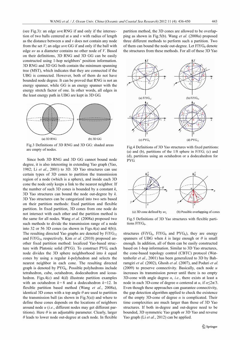
(see Fig.3): an edge uv∈RNG if and only if the intersec-tion of two balls centered at u and v with radius of length as the distance between u and v does not contain any node from the set V; an edge uv∈GG if and only if the ball with edge uv as a diameter contains no other node of V. Based on their definitions, 3D RNG and 3D GG can be easily constructed using 1-hop neighbors’ position information. 3D RNG and 3D GG both contain the minimum spanning tree (MST), which indicates that they are connected if the UBG is connected. However, both of them do not have bounded node degree. It can be proved that RNG is not an energy spanner, while GG is an energy spanner with the energy stretch factor of one. In other words, all edges in the least energy path in UBG are kept in 3D GG.

Fig.3 Definitions of 3D RNG and 3D GG: shaded areas are empty of nodes.

Since both 3D RNG and 3D GG cannot bound node degree, it is also interesting in extending Yao graph (Yao, 1982; Li et al., 2001) to 3D. 3D Yao structures can use certain types of 3D cones to partition the transmission region of a node (which is a sphere), and inside each 3D cone the node only keeps a link to the nearest neighbor. If the number of such 3D cones is bounded by a constant k, 3D Yao structures can bound the node out-degree by k. 3D Yao structures can be categorized into two sets based on their partition methods: fixed partition and flexible partition. In fixed partition, 3D cones from one node do not intersect with each other and the partition method is the same for all nodes. Wang et al. (2008a) proposed two such methods to divide the transmission range of a node into 32 or 56 3D cones (as shown in Figs.4(a) and 4(b)). The resulting directed Yao graphs are denoted by FiYG32 and FiYG56 respectively. Kim et al. (2010) proposed an-other fixed partition method: localized Yao-based struc-ture with Platonic solid (PYG). To construct PYG, each node divides the 3D sphere neighborhood into k equal cones by using a regular k-polyhedron and selects the nearest neighbor in each cone. The resulting directed graph is denoted by PYGk. Possible polyhedrons include tetrahedron, cube, octahedron, dodecahedron and icosa-hedron. Figs.4(c) and 4(d) illustrate partition examples with an octahedron k = 8 and a dodecahedron k =12. In flexible partition based method (Wang et al., 2008a), identical 3D cones with a top angle θ are used to partition the transmission ball (as shown in Fig.5(a)) and where to define these cones depends on the locations of neighbors around node u (i.e., different nodes may get different par-titions). Here θ is an adjustable parameter. Clearly, larger θ leads to lower node out-degree at each node. In flexible

partition method, the 3D cones are allowed to be overlap-ping as shown in Fig.5(b). Wang et al. (2008a) proposed three different methods to perform such a partition. Two of them can bound the node out-degree. Let FlYGθ denote the structures from these methods. For all of these 3D Yao

Fig.4 Definitions of 3D Yao structures with fixed partitions: (a) and (b), partitions of the 1/8 sphere in FiYG; (c) and (d), partitions using an octahedron or a dodecahedron for PYG.

Fig.5 Definitions of 3D Yao structures with flexible parti-tions FlYGθ.

structures (FiYGk, FlYGθ and PYGk), they are energy spanners of UBG when k is large enough or θ is small enough. In addition, all of them can be easily constructed based on 1-hop information. Similar to 3D Yao structures, the cone-based topology control (CBTC) protocol (Wat-tenhofer et al., 2001) has been generalized to 3D by Bah-ramgiri et al. (2002), Ghosh et al. (2007), and Poduri et al. (2009) to preserve connectivity. Basically, each node u increases its transmission power until there is no empty 3D-cone with angle degree α, i.e., there exists at least a node in each 3D-cone of degree α centered at u, if α≤2π/3. Even though these approaches can guarantee connectivity, the gap detection algorithm applied to check the existence of the empty 3D-cone of degree α is complicated. Their time complexities are much larger than those of 3D Yao structures. If both in-degree and out-degree need to be bounded, 3D symmetric Yao graph or 3D Yao and reverse Yao graph (Li et al., 2012) can be applied.


444

So far, we have introduced several localized 3D geo-metric structures. Some of them have bounded node de-gree, and some of them are energy spanners of UBG. No-tice that all listed topologies only need 1-hop neighbor information to be constructed, i.e., all construction algo-rithms are localized algorithms. Thus, when nodes move, the updates of these topologies can be efficiently per-formed in a local area without any global affects.

5.4 Handling Fault Tolerance and Shadow Zone

In order to be power efficient, traditional topology con-trol algorithms try to reduce the number of links, and thereby reduce the redundancy available for tolerating node and link failures. Thus, the topology derived from such algorithms is more vulnerable to node failures or link breakages. Fortunately, most of the 3D structures we introduced so far can be easily extended to support fault tolerance. To achieve both sparseness and fault tolerance, Wang et al. (2009) extended 3D RNG, 3D GG, and 3D Yao structures to support fault tolerance by a simple modification of their definitions. The new 3D topologies not only guarantee k-connectivity of the network, but also ensure the bounded node degree and constant energy stretch factor even under k-1 node failures. A similar idea has been used by Bahramgiri et al. (2002) for 3D CBTC.

The spatially-variant underwater channel can also cause the formation of shadow zones, which are time-variant areas where there is little signal propagation energy due to the refraction of signals by the sound speed fluctuation (Preisig, 2007). Shadow zones can cause high bit error rates, losses of connectivity and dramatically impact communications performance. Domingo (2009) proposed a distributed adaptive topology reorganization scheme that alleviates the effects of energy limitations and is able to maintain connectivity between sensor nodes in 3D un-derwater sensor networks in the presence of shadow zones. It can estimate when the shadow zones have dis-appeared using double sensor units to re-establish com-munication very quickly through the original acoustic wireless links.

6 3D Position-Based Routing

Routing is another challenging task in ocean sensor networks, which aims to delivery packets from a source node to a destination node via multihop relays. Pompili and Akyildiz (2009) have shown that traditional terrestrial routing solutions (such as classical proactive and reactive protocols) may not be suitable for underwater networks due to slow propagation of acoustic signals and high la-tency of path establishment and maintenance. The geo-metric nature of the multi-hop sensor networks provides a promising idea: position-based routing (also called geo-metric routing, georouting, or geographic routing). Posi-tion-based routing protocols do not need the dissemina-tion of route discovery information, and no routing tables are maintained at each node. They only use the local po-sition information at each node and geometric properties

of surrounding neighbors to determine how to route the packet. This leads to lower overhead and higher scalabil-ity, and makes such routing protocols suitable for ocean sensor networks. In this section, we focus on reviewing different 3D position-based routing techniques to achieve sustainability and scalability in large-scale 3D sensor networks. Many of them can be directly used in 3D ocean sensor networks. Notice that there are also other types of routing solutions (no position information is used) for 3D ocean sensor networks; however, due to space limitation we could not include them within this survey.

6.1 3D Greedy Routing

Most classical and widely used position-based routing is greedy routing, in which a packet is greedily forwarded to the closest node to the destination in order to minimize the average hop count. Greedy routing can be easily ex-tended to 3D cases. Actually, several under-water routing protocols (Pompili and Melodia, 2005; Xie et al., 2006) for underwater sensor networks are just variations of 3D greedy routing. Fig.6 illustrates the basic idea of 3D greedy routing. Let t be the destination node. As shown in Fig.6(a), current node u finds the next relay node v that is the closest to t among all neighbors of u. But, it is easy to construct an example (see Fig.6(b)) to show that greedy routing will not succeed to reach the destination but fall into a local minimum (at a node without any ‘better’ or ‘closer’ neighbors). This is true for both 2D and 3D net-works. To guarantee packet delivery of 3D greedy routing is not straightforward and much more challenging than in 2D greedy routing. In 2D networks, face routing can be used on planar topology to recover from the local mini-mum of greedy routing and guarantee the delivery (Bose et al., 1999). However, there is no planar topology con-cept any more in 3D networks, thus, face routing cannot be applied directly to help 3D greedy routing get out of local minimum. Most importantly, Durocher et al. (2008) have proved that there is no deterministic localized rout-ing algorithm for general 3D networks that guarantees the delivery of packets. Here, a routing algorithm is localized if the decision to which node to forward a packet is based only on: the information in the header of the packet and the local information gathered by the node from a small neighborhood (i.e. 1-hop neighbors of the node).

One simple way to guarantee the packet delivery for greedy routing in 3D networks is letting all nodes have sufficiently large transmission range to avoid the exis-tence of local minimum. It is clear that this can be achieved when the transmission range is infinite. Given a set of sensors V in a 3D sensor network, let the critical transmission range (CTR) for 3D greedy routing be the smallest transmission range that can guarantee the deliv-ery of packets between any source-destination pair of nodes among V. Wang et al. (2008b, 2010) studied the CTR of 3D greedy routing in large-scale random 3D networks. When a set V of n sensor nodes uniformly dis-tributed in a compact and convex 3D region with unit-

volume and each node has a uniform transmission range


445

rn , the CTR for 3D greedy routing is asymptotic almost surely at most 3 3 ln /(4π )n nβ for any β > β0 and at least 3 3 ln /(4π )n nβ for any β < β0, where β0 = 3.2. This theo-retical result answers a fundamental question about how large the transmission range should be set in a 3D sensor networks, such that 3D greedy routing guarantees the delivery of packets between any two nodes.

Fig.6 Illustration of 3D greedy routing.

6.2 3D Routing via Mapping and Projection

Since face routing can always find a detour out of the local minimum for greedy routing in planar 2D networks (Bose et al., 1999), it is natural to project the 3D network onto a 2D space (as shown in Fig.7(a)) and use face rout-ing in the 2D plane. Kao et al. (2005) and Abdallah et al. (2007) have proposed several 3D position-based routing protocols using this idea. However, as shown in Fig.7(b) (Kao et al., 2005), a planar graph cannot be extracted from the projected graph. It is clear that removing either v′1v′2 or v′3v′4 will break the connectivity. Kao et al. (2005) and Abdallah et al. (2007) also proposed face coordinate routing (CFace) which first projects the network onto the xy plane and runs face routing on it. If the face routing fails on the projected graph, it will project the network onto the second plane (the yz plane). If the face routing fails again, the network is projected onto the third plane (the xz plane). However, if the face routing fails on the third plane, this method fails. In 2D, several greedy em-bedding algorithms (Kleinberg, 2007; Zhang et al., 2007; Sarkar et al., 2009) can embed the 2D network into cer-tain space such that greedy routing guarantees delivery in the new virtual space. Unfortunately, none of the greedy embedding algorithms in the literature can be extended from 2D to 3D general networks.

Fig.7 Simple projection from 3D to 2D does not work.

6.3 Randomized 3D Greedy Routing

Since no deterministic localized position-based routing can guarantee the packet delivery (Durocher et al., 2008),

randomized algorithms become possible solutions. Ab-dallah et al. (2006) proposed a new randomized posi-tion-based routing for 3D networks, called randomized AB3D routing. AB3D algorithm selects the next hop x randomly from three candidate neighbors of the current node u (the node nearest to the destination t (denoted by a), the node chosen by 3D greedy from all neighbors of u above or below the plane defined by a, u and t. The probabilities to choose x from these three candidates could be the same or related to their angles or distances to the destination. However, such routing method does not have any performance guarantee. Flury and Wattenhofer (2008) explored using random walks to escape from the local minimum and proposed a greedy-random-greedy routing method. The packet is first forwarded greedily until a local minimum is encountered. To resolve the local minimum, a randomized recovery algorithm based on random walks kicks in. Whereas a packet moving around randomly in the network may seem very inefficient and too simplistic, they do propose several techniques to make random walks more efficient. They proved that the expected number of hops needed for the random walk method is in the square of the optimal localized routing algorithm. However, in practice, this randomized method still often leads to high overhead or long delay in 3D networks.

6.4 3D Greedy Routing over Constructed Structures

Guarantee delivery can also be achieved at the cost of more (non-constant-bounded) storage space by construct-ing certain routing structures. For example, Lam and Qian (2011) used a virtual Delaunay triangulation to aid posi-tion-based routing, while Zhou et al. (2010) used hull tree structures (spanning trees) to store possible routes around the void.

Lam and Qian (2011) proposed multi-hop Delaunay triangulation (MDT) routing over a virtual Delaunay tri-angulation. In a d-dimensional Euclidean space, a Delau-nay triangulation is a triangulation such that there is no point in V inside the circum-hypersphere of any d- sim-plex. In 3D space, the 3-simplex is a tetrahedron. Morin (2001) has proved that 2D greedy routing can guarantee the packet delivery on 2D Delaunay triangulation. This is also true in 3D space. However, building the Delaunay triangulation needs global information and the length of a Delaunay edge could be longer than the maximum trans-mission range. The key idea of the MDT method is to relax the requirement that every node be able to commu-nicate directly with its neighbor in Delaunay triangulation. In a MDT, the neighbor of a node may not be a physical neighbor. A virtual link represents a multi-hop path be-tween them. When the current node u has a packet with destination t, it forwards the packet to a physical neighbor closest to t if u is not a local minimum; otherwise the packet is forwarded via a virtual link to a multi-hop De-launay neighbor closest to t. MDT can guarantee the packet delivery using a finite number of hops. However, the construction and maintenance of the MDT at each


446

node are not purely localized. Zhou et al. (2010) also proposed a position-based rout-

ing method (3D Greedy Distributed Spanning Tree Rout-ing, GDSTR-3D), which uses two hull trees (both span-ning trees) for recovery from local minimums. For each tree, each node stores two 2D convex hulls to aggregate the locations of all descendants in the subtrees rooted at the node. The two 2D convex hulls approximate a 3D convex hull at each node to save the storage space. GDSTR-3D forwards packets greedily as long as it can find a neighbor closer to the destination than the current node. If the packet ends up in a local minimum, the node then attempts to forward the packet to a neighbor that has a neighbor closer to the destination than itself. If this 2-hop greedy routing still fails, GDSTR-3D switches to forwarding the packet along the edges of a spanning tree which aggregates the location of the nodes in its subtrees using two 2D convex hulls. Since the spanning tree can always reach the destination if the network is connected, GDSTR-3D can always guide the packet to escape from the local minimum and guarantee the delivery. However, in the worst case routing with the hull tree degrades to depth first search, so the routing path could be long and the storage in a node can be very large. In addition, some nodes (such as the roots of trees) will be heavily loaded.

6.5 Hybrid 3D Greedy Routing

There are also hybrid greedy routing methods which combine various solutions above. For example, Abdallah et al. (2006) also combined their randomized routing method with the projection-based face routing (Kao et al., 2005; Abdallah et al., 2007). Xia et al. (2011) recently proposed a hybrid 3D greedy routing, which uses both a constructed routing structure (unit tetrahedron cell) and a projection method (volumetric harmonic mapping). We now briefly review their routing methods. First, a unit tetrahedron cell (UTC) mesh structure is constructed from all 3D nodes. A UTC is a tetrahedron formed by four network nodes, which does not intersect with any other

tetrahedrons. The union of all UTCs forms the mesh structure. Second, a face-based greedy routing is pro-posed to delivery packets within the internal (non- bound-ary) UTC. The idea is very like the face routing in 2D. The face-based greedy routing will pass a sequence of faces which intersect with the line segment between the source and destination. It can be proved that such face-

based greedy routing does not fail at a non-boundary UTC. Third, to handle the possible failure of greedy routing at boundaries, the proposed method maps the whole UTC mesh using volumetric harmonic mapping under spherical boundary condition so that the boundary nodes are now on a surface of a sphere. This can guaran-tee the node-based greedy routing can reach any bound-ary node successfully. Last, a hybrid greedy routing is proposed, which alternately uses face-based greedy for internal UTCs and node-based greedy for boundary UTCs. Face-based greedy can guarantee the delivery in non-

boundary UTCs. When the packet fails at a boundary UTC, node-based greedy is applied to escape the void. Since the boundary has been mapped to a sphere, node-

based greedy routing always succeeds on a boundary. When it is possible, it switches back to face-based greedy to route the packet towards the destination. However, the complexity of this proposed method (such as spheri-cal/volumetric harmonic mapping) still makes it not very practical. In addition, how to handle multiple inner holes and routing across them is still not clear.

In this section, we briefly review existing geometric solutions for designing 3D position-based routing to guar-antee the packet delivery in 3D wireless sensor networks. Table 2 provides a summary and comparison of these solutions. Most of these techniques can be applied in static 3D ocean sensor networks. Note that certain per-formances of position-based routing protocols are relying on the accuracy of node position information. Therefore, 3D localization techniques we introduced in Section 4 are usually used together with 3D position-based routing in 3D ocean sensor networks. Beyond the goal of delivery

Table 2 Summary of existing geometric solutions for 3D position-based routing aiming to improve or guarantee the packet delivery in 3D wireless sensor networks

3D Position-based routing Enlarging TrX range

Projection-based method

Randomized method

Constructed structure

Hybrid Method

Localized method

Delivery guarantee

3D Greedy routing Yes CTR of 3D greedy routing in random networks (Wang et al., 2008b, 2010)

Yes Yes Yes (with high prob.)

Face coordinate routing (CFace) (Kao et al., 2005; Abdallah et al., 2007)

Yes (mapping to 2D)

Yes

Randomized AB3D routing (Abdallah et al., 2006)

Yes Yes

Hybrid AB3D-CFace routing (Abdal-lah et al., 2006)

Yes (mapping to 2D)

Yes Yes Yes

Greedy-random-greedy (Flury and Wattenhofer, 2008)

Yes Yes Yes

Multi-hop delaunay triangulation routing (Lam and Qian, 2011)

Yes (virtual Delau-nay triangulation)

Yes

Greedy distributed spanning tree routing GDSTR-3D (Zhou et al., 2010)

Yes (spanning trees) Yes

Volumetric harmonic mapping based greedy routing (Xia et al., 2011)

Yes (volumetric harmonic mapping)

Yes (unit tetrahedron cells)

Yes Yes


447

guarantee, there are also other design goals for 3D posi-tion-based routing, such as energy efficiency (Wang et al., 2011), robustness and reliability. In addition, there are other types of 3D routing protocols (such as delay tolerant routing protocols (Guo et al., 2010; Rahim et al., 2011)) for ocean/underwater sensor networks, which may not rely on the position information. Due to space limitation, we could not include them within this survey.

7 Conclusion

With the growing ocean applications, new 3D ocean sensor network systems have been developed and de-ployed in recent years. Due to the unique characteristics of underwater acoustic channels and the complex de-ployment environment in 3D ocean spaces, various effi-cient and reliable 3D communication and networking protocols have been proposed. In this paper, we present an overview of the most recent advances in network de-sign principles for 3D ocean sensor networks, with fo-cuses on deployment, localization, topology design, and position-based routing in 3D ocean spaces. We strongly believe that more promising developments and significant improvements of ocean sensor network systems will be achieved over the next decade. This will greatly enhance humans’ abilities in exploration and exploitation of the ocean.

Acknowledgements

The work of Y. Wang was supported in part by the US National Science Foundation (NSF) under Grant Nos. CNS-0721666, CNS-0915331, and CNS-1050398. The work of Y. Liu was partially supported by the National Natural Science Foundation of China (NSFC) under Grant No. 61074092 and by the Shandong Provincial Natural Science Foundation, China under Grant No. Q2008E01. The work of Z. Guo was partially supported by the NSFC under Grant Nos. 61170258 and 6093301. This work was partially done when Y. Liu visited the De-partment of Computer Science, University of North Caro-lina at Charlotte, with a scholarship from the China Scholarship Council.

References Abdallah, A., Fevens, T., and Opatrny, J., 2006. Randomized 3D

position-based routing algorithms for ad hoc networks. The Third Annual International Conference on Mobile and Ubiq-uitous Systems: Networking & Services. 1-8, DOI: 10. 1109/

MOBIQ.2006.340457. Abdallah, A., Fevens, T., and Opatrny, J., 2007. Power-aware

3D position-based routing algorithm for ad hoc networks. Proceeding of IEEE International Conference on Communi-cations (ICC '07). 3130-3135, DOI: 10.1109/ICC.2007.519.

Akkaya, K., and Newell, A., 2009. Self-deployment of sensors for maximized coverage in underwater acoustic sensor net-works. Computer Communications, 32 (7): 1233-1244, DOI: 10.1016/j.comcom.2009.04.002.

Akyildiz, I. F., Pompili, D., and Melodia, T., 2005. Underwater

acoustic sensor networks: research challenges. Ad Hoc Net-works, 3 (3): 257-279, DOI: 10.1016/j.adhoc.2005.01.004.

Akyildiz, I. F., Pompili, D., and Melodia, T., 2007. State of the art in protocol research for underwater acoustic sensor net-works. Mobile Computing and Communications Review, 11 (4): 11-22, DOI: 10.1145/1347364.1347371.

Alam, S. M. N., and Haas, Z. J., 2006. Coverage and connec-tivity in three-dimensional networks. Proceeding of the 12th annual international conference on Mobile computing and networking (MobiCom '06). 346-357, DOI: 10.1145/ 1161089.

1161128. Alam, S. M. N., and Haas, Z. J., 2010. Hierarchical and nonhi-

erarchical three-dimensional underwater wireless sensor net-works. The Computing Research Repository (CoRR), Vol. abs/1005.3073, 21pp.

Ammari, H. M., and Das, S. K., 2010. A study of k-coverage and measures of connectivity in 3D wireless sensor networks. IEEE Transactions on Computers, 59 (2): 243-257, DOI: 10.

1109/TC.2009.166. Argo Science Team, 1998. On the Design and Implementation

of Argo. http://www.argo.ucsd.edu. Aslam, N., and Robertson, W., 2010. Distributed coverage and

connectivity in three dimensional wireless sensor networks. Proceeding of the 6th International Wireless Communications and Mobile Computing Conference (IWCMC '10). 1141- 1145, DOI: 10.1145/1815396.1815657.

Bahramgiri, M., Hajiaghayi, M.-T., and Mirrokni, V. S., 2002. Fault-tolerant and 3-dimensional distributed topology control algorithms in wireless multi-hop networks. Proceeding of the 11th International Conference on Computer Communications and Networks. 392-397, DOI: 10.1109/ICCCN.2002. 1043097.

Bai, X., Zhang, C., Xuan, D., and Jia, W., 2009a. Full-coverage and k-connectivity (k=14, 6) three dimensional networks. Proceeding of the 28th IEEE International Conference on Computer Communications (INFOCOM 2009). 388-396, DOI: 10. 1109/INFCOM.2009.5061943.

Bai, X., Zhang, C., Xuan, D., Teng, J., and Jia, W., 2009b. Low-connectivity and full-coverage three dimensional wire-less sensor networks. Proceeding of the tenth ACM interna-tional symposium on Mobile ad hoc networking and comput-ing (MobiHoc '09). 145-154, DOI: 10.1145/1530748. 1530768.

Barr, S., Wang, J., and Liu, B., 2011. An efficient method for constructing underwater sensor barriers. Journal of Commu-nications, 6 (5): 370-383, DOI: 10.4304/jcm.6.5.370-383.

Bose, P., Morin, P., Stojmenović, I., and Urrutia, J., 1999. Rout-ing with guaranteed delivery in ad hoc wireless networks. Proceeding of the 3rd International Workshop on Discrete Algorithms and Methods for Mobile Computing and Commu-nications (DIALM '99). 48-55, DOI: 10.1145/313239.313282.

Cayirci, E., Tezcan, H., Dogan, Y., and Coskun, V., 2006. Wire-less sensor networks for underwater surveillance systems. Ad Hoc Networks, 4 (4): 431-446, DOI: 10.1016/j.adhoc.2004.10.

008. Chen, K., Zhou, Y., and He, J., 2009. A localization scheme for

underwater wireless sensor networks. International Journal of Advanced Science and Technology, 4: 9-16, DOI: 10.1.1. 178.3027.

Cheng, W., Thaeler, A., Cheng, X., Liu, F., Lu, X., and Lu, Z., 2009. Time-synchronization free localization in large scale underwater acoustic sensor networks. Proceeding of the 29th IEEE International Conference on Distributed Computing Systems Workshops. 80-87, DOI: 10.1109/ICDCSW.2009. 79.

Cheng, X., Shu, H., Liang, Q., and Du, D. H.-C., 2008. Silent positioning in underwater acoustic sensor networks. IEEE


448

Transactions on Vehicular Technology, 57 (3): 1756-1766, DOI: 10.1109/TVT.2007.912142.

Chitre, M., Shahabudeen, S., and Stojanovic, M., 2008. Under-water acoustic communications and networking: recent ad-vances and future challenges. Marine Technology Society Journal, 42 (1): 103-116, DOI: 10.4031/002533208786861263.

Cui, J.-H., Kong, J., Gerla, M., and Zhou, S., 2006. The chal-lenges of building mobile underwater wireless networks for aquatic applications. IEEE Network, 20 (3): 12-18, DOI: 10.

1109/MNET.2006.1637927. Curtin, T. B., and Bellingham, J. G., 2009. Progress toward

autonomous ocean sampling networks. Deep-Sea Research Part II, 56 (3): 62-67, DOI: 10.1016/j.dsr2.2008.09.005.

Curtin, T. B., Bellingham, J. G., Catipovic, J., and Webb, D., 1993. Autonomous oceanographic sampling networks. Ocean-ography, 6 (3): 86-94.

Detweiler, C., Doniec, M., Vasilescu, I., Basha, E., and Rus, D., 2012. Autonomous depth adjustment for underwater sensor networks: design and applications. IEEE/ASME Transactions on Mechatronics, 17 (1): 16-24, DOI: 10.1109/TMECH.2011.

2175003. Domingo, M. C., 2009. A Topology reorganization scheme for

reliable communication in underwater wireless sensor net-works affected by shadow zones. Sensors, 9 (11): 8684-p8708, DOI: 10.3390/s91108684.

Durocher, S., Kirkpatrick, D., and Narayanan, L., 2008. On routing with guaranteed delivery in three-dimensional ad hoc wireless networks. Proceeding of the 9th Int’l Conference on Distributed Computing and Networking (ICDCN 2008), Lec-ture Notes in Computer Science. Volume 4904/2008, 546- 557, DOI: 10.1007/978-3-540-77444-0_58.

Erol, M., Vieira, L. F. M., and Gerla, M., 2007a. Localization with Dive'N'Rise (DNR) beacons for underwater acoustic sensor networks. Proceeding of the second workshop on Un-derwater networks (WuWNet '07). 97-100, DOI: 10.1145/

1287812.1287833. Erol, M., Vieira, L. F. M., and Gerla, M., 2007b. Auv-aided

localization for underwater sensor networks. Proceeding of International Conference on Wireless Algorithms, Systems and Applications (WASA 2007). 44-54, DOI: 10.1109/WASA.

2007.34. Erol, M., Vieira, L. F. M., Caruso, A., Paparella, F., Gerla, M.,

and Oktug, S., 2008. Multi stage underwater sensor localiza-tion using mobile beacons. Proceeding of the 2nd Interna-tional Conference on Sensor Technologies and Applications (SENSORCOMM '08). 710-714, DOI: 10.1109/SENSORCO

MM.2008.32. Erol-Kantarciz, M., Mouftah, H. T., and Oktug, S., 2011. A sur-

vey of architectures and localization techniques for underwa-ter acoustic sensor networks. IEEE Communications Surveys and Tutorials, 13 (3): 487-502, DOI: 10.1109/SURV.2011.

020211.00035. Flury, R., and Wattenhofer, R., 2008. Randomized 3D Geo-

graphic Routing. Proceeding of the 27th IEEE International Conference on Computer Communications (INFOCOM 2008). 834-842, DOI: 10.1109/INFOCOM.2008.135.

Gabriel, K. R., and Sokal, R. R., 1969. A new statistical ap-proach to geographic variation analysis. Systematic Biology, 18 (3): 259-278, DOI: 10.2307/2412323.

Ghosh, A., Wang, Y., and Krishnamachari, B., 2007. Efficient distributed topology control in 3-dimensional wireless net-works. Proceeding of the 4th Annual IEEE Communications Society Conference on Sensor, Mesh and Ad Hoc Communi-cations and Networks (SECON '07). 91-100, DOI: 10. 1109/

SAHCN.2007.4292821. Glenn, S. M., Schofield, O. M., Chant, R., Kohut, J., McDonnell,

J., and McLean. S. D., 2006. The leo-15 costal cabled obser-vatory – Phase II for the next evolutionary decade of ocean-ography. SSC06-Scientific Submarine Cable, 2006, 1-6.

Guo, Z., Hong, F., Feng, Y., Chen, P., Yang, X., and Jiang, M., 2008. OceanSense: sensor network of realtime ocean envi-ronmental data observation and its development platform. Proceeding of the 3rd ACM International Workshop on Un-der Water Networks (WUWNet). New York, 23-24.

Guo, Z., Wang, B., and Cui, J.-H., 2010. Prediction assisted single-copy routing in underwater delay tolerant networks. Proceeding of the 2010 IEEE Global Telecommunications Con- ference (GLOBECOM 2010). 1-6, DOI: 10.1109/ GLOCOM.

2010.5683232. Han, G., Jiang, J., Shu, L., Xu, Y., and Feng W., 2012. Localiza-

tion algorithms of underwater wireless sensor networks: A sur-vey. Sensors, 12 (2): 2026-2061, DOI: 10.3390/s120202026.

Heidemann, J., Stojanovic, M., and Zorzi, M., 2012. Underwater sensor networks: applications, advances and challenges. Phi-losophical Transactions of the Royal Society A, 370 (1958): 158-175, DOI: 10.1098/rsta.2011.0214

Howe, B., and McGinnis, T., 2004. Sensor networks for cabled ocean observatories. Proceeding of 2004 International Sym-posium on Underwater Technology (UT '04). 113-120, DOI: 10. 1109/UT.2004.1405499.

Isbitiren, G., and Akan, O. B., 2011. Three-dimensional under-water target tracking with acoustic sensor networks. IEEE Transactions on Vehicular Technology, 60 (8): 3897-3906, DOI: 10.1109/TVT.2011.2163538.

Isik, M. T., and Akan, O. B., 2009. A three dimensional localiza-tion algorithm for underwater acoustic sensor networks. IEEE Transactions on Wireless Communications, 8 (9): 4457-4463, DOI: 10.1109/TWC.2009.081628.

Kao, G. S.-C., Fevens, T., and Opatrny, J., 2005. Position-based routing on 3-D geometric graphs in mobile ad hoc networks. Proceeding of the 17th Canadian Conference on Computa-tional Geometry (CCCG’05). 81-91.

Kim, J., Shin, J., and Kwon, Y., 2010. Adaptive 3-dimensional topology control for wireless ad-hoc sensor networks. IEICE Transactions on Communications, E93.B (11): 2901-2911, DOI: 10.1587/transcom.E93.B.2901.

Kleinberg, R., 2007. Geographic routing using hyperbolic space. Proceeding of the 26th IEEE International Conference on Computer Communications (INFOCOM 2007). 1902-1909, DOI: 10.1109/INFCOM.2007.221.

Lam, S. S., and Qian, C., 2011. Geographic routing in d-dimensional spaces with guaranteed delivery and low stretch. Proceeding of the ACM SIGMETRICS joint interna-tional conference on Measurement and modeling of computer systems (SIGMETRICS '11). 257-268, DOI: 10.1145/ 1993744.

1993770. Li, F., Chen, Z., and Wang, Y., 2012. Localized geometric to-

pologies with bounded node degree for three-dimensional wireless sensor networks. EURASIP Journal on Wireless Communications and Networking, Volume 2012, Issue 1, Ar-ticle ID: 157, DOI: 10.1186/1687-1499-2012-157.

Li, X.-Y., Wan, P.-J., and Wang, Y., 2001. Power efficient and sparse spanner for wireless ad hoc networks. Proceeding of the 10th International Conference on Computer Communica-tions and Networks (ICCCN '01). 564-567, DOI: 10. 1109/

ICCCN. 2001.956322. Luo, H., Guo, Z., Dong, W., Hong, F., and Zhao, Y., 2010. LDB:

Localization with directional beacons for sparse 3d underwa-


449

ter acoustic sensor networks. Journal of Networks, 5 (1): 28-

38, DOI: 10.4304/jnw.5.1.28-38. Manum, H., and Schmid, M., 2007. Monitoring in a harsh envi-

ronment. Control & Automation, 18 (5): 22-27. Mirza, D., and Schurgers, C., 2007. Collaborative localization

for fleets of underwater drifters. Proceeding of OCEANS 2007. 1-6, DOI: 10.1109/OCEANS.2007.4449391.

Mirza, D., and Schurgers, C., 2008. Motion-aware self- localiza-tion for underwater networks. Proceeding of the third ACM international workshop on Underwater Networks (WuWNeT '08). 51-58, DOI: 10.1145/1410107.1410117.

Mohamed, N., Jawhar, I., Al-Jaroodi, J., and Zhang, L., 2011. Sensor network architectures for monitoring underwater pipe-lines. Sensors, 11 (11): 10738-10764, DOI: 10.3390/s11111

0738. Morin, P. R., 2001. Online routing in geometric graphs. PhD

Thesis, School of Computer Science, Carleton University. Paley, D. A., Zhang, F., and Leonard, N. E., 2008. Cooperative

control for ocean sampling: the glider coordinated control system. IEEE Transactions on Control System Technology, 16 (4): 735-744, DOI: 10.1109/TCST.2007.912238.

Poduri, S., Pattem, S., Krishnamachari, B., and Sukhatme, G. S., 2009. Using local geometry for tunable topology control in sensor networks. IEEE Transactions on Mobile Computing, 8 (2): 218-230, DOI: 10.1109/TMC.2008.95.

Pompili, D., and Akyildiz, I. F., 2009. Overview of networking protocols for underwater wireless communications. IEEE Communications Magazine, 47 (1): 97-102, DOI: 10.1109/

MCOM.2009.4752684. Pompili, D., and Melodia, T., 2005. Three-dimensional routing

in underwater acoustic sensor networks. Proceeding of the 2nd ACM international workshop on Performance evaluation of wireless ad hoc, sensor, and ubiquitous networks (PE-

WASUN '05). 214-221, DOI: 10.1145/1089803.1089988. Pompili, D., Melodia, T., and Akyildiz, I. F., 2009. Three- di-

mensional and two-dimensional deployment analysis for un-derwater acoustic sensor networks. Ad Hoc Networks, 7 (4): 778-790, DOI: 10.1016/j.adhoc.2008.07.010.

Preisig, J., 2007. Acoustic propagation considerations for un-derwater acoustic communications network development. ACM SIGMOBILE Mobile Computing and Communications Review, 11 (4): 2-10, DOI: 10.1145/1347364.1347370.

Rahim, M. S., Casari, P., Guerra, F., and Zorzi, M., 2011. On the performance of delay-tolerant routing protocols in underwater networks. Proceeding of the 2011 IEEE OCEANS. 1-7, DOI: 10.1109/Oceans-Spain.2011.6003388.

Rice, J. A., 2007. US navy Seaweb development. Proceeding of the Second Workshop on Underwater Networks (WuWNet '07). 3-4, DOI: 10.1145/1287812.1287814.

Sarkar, R., Yin, X., Gao, J., Luo, F., and Gu, X. D., 2009. Greedy routing with guaranteed delivery using ricci flows. Proceeding of the 2009 International Conference on Informa-tion Processing in Sensor Networks (IPSN’09). 121-132.

Sozer, E. M., Stojanovic, M., and Proakis, J. G., 2000. Under-water acoustic networks. IEEE Journal of Oceanic Engineer-ing, 25 (1): 72-83, DOI: 10.1109/48.820738.

Tan, H.-P., Diamant, R., Seah, W. K.G., and Waldmeyer, M., 2011. A survey of techniques and challenges in underwater localization. Ocean Engineering, 38 (14-15): 1663-1676, DOI: 10.1016/j.oceaneng.2011.07.017.

Tan, H.-P., Gabor, A. F., Eu, Z. A., and Seah, W. K. G., 2010. A wide coverage positioning system (WPS) for underwater lo-calization. Proceeding of 2010 IEEE International Confer-ence on Communications (IEEE ICC 2010). 1-5, DOI: 10.

1109/ ICC.2010.5501950. Teymorian, A. Y., Cheng, W., Ma, L., Cheng, X., Lu, X., and Lu,

Z., 2009. 3D underwater sensor network localization. IEEE Transactions on Mobile Computing, 8 (12): 1610-1621, DOI: 10.1109/TMC.2009.80.

Toussaint, G. T., 1980. The relative neighborhood graph of a finite planar set. Pattern Recognition, 12 (4): 261-268, DOI: 10.1016/0031-3203(80)90066-7.

Wang, Y., 2008. Topology control for wireless sensor networks. In: Wireless Sensor Networks and Applications (Chapter 5). Li, Y., et al., eds., Springer, 441pp.

Wang, Y., 2013. Three-dimensional wireless sensor networks: geometric approaches for topology and routing design. In: The Art of Wireless Sensor Networks. Ammari, H. M., ed., Springer, to published.

Wang, Y., and Li, L., 2009. Localization in wireless sensor net-works. In: RFID and Sensor Networks: Architectures, Proto-cols, Security and Integrations. Zhang, Y., et al., eds., Auer-bach Publications, Taylor & Francis Group, 646pp.

Wang, Y., Cao, L., Dahlberg, T. A., Li, F., and Shi, X., 2009. Self-organizing fault-tolerant topology control in large-scale three-dimensional wireless networks. ACM Transactions on Autonomous and Adaptive Systems, 4 (3), Article 19, 21pp. DOI: 10.1145/1552297.1552302.

Wang, Y., Li, F., and Dahlberg, T. A., 2008a. Energy-efficient topology control for three-dimensional sensor networks. In-ternational Journal of Sensor Networks, 4 (1-2): 68-78, DOI: 10.1504/IJSNet.2008.019253.

Wang, Y., Li, X.-Y., Song, W.-Z., Huang, M., and Dahlberg, T. A., 2011. Energy-efficient localized routing in random multi-hop wireless networks. IEEE Transactions on Parallel and Distributed Systems, 22 (8): 1249-1257, DOI: 10.1109/TPDS.

2010.198. Wang, Y., Yi, C.-W., and Li, F., 2008b. Delivery guarantee of

greedy routing in three dimensional wireless networks. Pro-ceeding of International Conference on Wireless Algorithms, Systems and Applications (WASA08), Lecture Notes in Com-puter Science. Volume 5258/2008, 4-16, DOI: 10.1007/ 978-3-

540-88582-5_4. Wang, Y., Yi, C.-W., Huang, M., and Li, F., 2010. Three- dimen-

sional greedy routing in large-scale random wireless sensor networks. Ad Hoc Networks, DOI: 10.1016/j.adhoc.2010.10.

003. Watfa, M. K., and Commuri, S., 2006a. The 3-dimensional

wireless sensor network coverage problem. Proceeding of the 2006 IEEE International Conference on Networking, Sensing and Control (ICNSC '06). 856-861, DOI: 10.1109/ ICNSC.

2006.1673259. Watfa, M. K., and Commuri, S., 2006b. Optimal 3-dimensional

sensor deployment strategy. Proceeding of the 3rd IEEE Consumer Communications and Networking Conference (CCNC 2006). 892-896, DOI: 10.1109/CCNC.2006.1593167.

Wattenhofer, R., Li, L., Bahl, P., and Wang, Y.-M., 2001. Dis-tributed topology control for power efficient operation in multihop wireless ad hoc networks. Proceeding of the 20th IEEE International Conference on Computer Communications (INFOCOM 2001). 1388-1397, DOI: 10.1109/INFCOM. 2001. 916634.

Weisberg, R. H., Barth, A., Alvera-Azcárate, A., and Zheng, L., 2009. Review: A coordinated coastal ocean observing and modeling system for the West Florida Continental Shelf. Harmful Algae, 8 (4): 585-597, DOI: 10.1016/j.hal.2008.11.

003. Xia, S., Yin, X., Wu, H., Jin, M., and Gu, X. D., 2011. Determi-


450

nistic greedy routing with guaranteed delivery in 3D wireless sensor networks. Proceeding of the 12th ACM International Symposium on Mobile Ad Hoc Networking and Computing (MobiHoc '11). 1-10, DOI: 10.1145/2107502.2107504.

Xie, P., Cui, J.-H., and Lao, L., 2006. VBF: vector-based for-warding protocol for underwater sensor networks. Proceedings of IFIP Networking’06, Lecture Notes in Computer Science. Volume 3976/2006, 1216-1221, DOI: 10.1007/11753810_111.

Yao, A. C.-C., 1982. On constructing minimum spanning trees in k-dimensional spaces and related problems. SIAM Journal on Computing, 11 (4):721-736.

Zhang, F., Li, H., Jiang, A., Chen, J., and Luo, P., 2007. Face tracing based geographic routing in nonplanar wireless net-works. Proceeding of the 26th IEEE International Conference on Computer Communications (INFOCOM 2007). 2243-2251, DOI: 10.1109/INFCOM.2007.259.

Zhang, S., Yu, J., Zhang, A., Yang, L., and Shu, Y., 2012. Marine vehicle sensor network architecture and protocol designs for ocean observation. Sensors, 12 (1): 373-390, DOI: 10.3390/ s120100373.

Zhou, J., Chen, Y., Leong, B., and Sundaramoorthy, P. S., 2010. Practical 3D geographic routing for wireless sensor networks. Proceeding of the 8th ACM Conference on Embedded Net-worked Sensor Systems (SenSys '10). 337-350, DOI: 10.1145/

1869983.1870016. Zhou, Y., Gu, B., Chen, K., Chen, J., and Guan, H., 2009. An

range-free localization scheme for large scale underwater wireless sensor networks. Journal of Shanghai Jiaotong Uni-versity, 14 (5): 562-568, DOI: 10.1007/s12204-009-0562-9.

Zhou, Z., Cui, J.-H., and Bagtzoglou, A., 2008. Scalable local-ization with mobility prediction for underwater sensor net-works. Proceeding of the 27th IEEE International Conference on Computer Communications (INFOCOM 2008). 2198-2206, DOI: 10.1109/INFOCOM.2008.287.

Zhou, Z., Cui, J.-H., and Zhou, S., 2007. Localization for large-scale underwater sensor networks. Proceeding of the 6th International IFIP-TC6 Conference on Ad Hoc and Sensor Networks, Wireless Networks, Next Generation Internet (NET- WORKING '07). 108-119.

(Edited by Xie Jun)

three-dimensional ocean sensor networks: a survey · ocean sensor network (osn), formed by...

Documents