three-dimensional magnetotelluric characterization of the ... · of the coso geothermal ﬁeld ......

Geothermics 37 (2008) 369–399

Available online at www.sciencedirect.com

Three-dimensional magnetotelluric characterizationof the Coso geothermal field

Gregory A. Newman a,∗, Erika Gasperikova a,G. Michael Hoversten b, Philip E. Wannamaker c

a Lawrence Berkeley National Laboratory, Earth Sciences Division,Berkeley, CA 94720, USA

b Chevron Energy Technology Company, Seismic Analysis and Property Estimation,San Ramon, CA 94583, USA

c Energy and Geoscience Institute, University of Utah, Salt Lake City,UT 84108, USA

Received 4 February 2008; accepted 5 February 2008Available online 14 April 2008

Abstract

A dense grid of 125 magnetotelluric (MT) stations plus a single line of contiguous bipole array profilinghas been acquired over the east flank of the Coso geothermal system, CA, USA. Due to production relatedelectromagnetic (EM) noise the permanent observatory at Parkfield, CA was used as a remote reference tosuppress this cultural EM noise interference. These data have been inverted to a fully three-dimensional (3D)resistivity model. This model shows the controlling geological structures possibly influencing well productionat Coso and correlations with mapped surface features such as faults and the regional geoelectric strike. The3D model also illustrates the refinement in positioning of resistivity contacts when compared to isolated 2Dinversion transects. The resistivity model has also been correlated with micro-earthquake locations, reservoirfluid production intervals and most importantly with an acoustic and shear velocity model derived by Wu andLees [Wu, H., Lees, J.M., 1999. Three-dimensional P and S wave velocity structures of the Coso GeothermalArea, California, from microseismic travel time data. J. Geophys. Res. 104 (B6), 13217–13233]. This latercorrelation shows that the near-vertical low-resistivity structure on the eastern flank of the producing field isalso a zone of increased acoustic velocity and increased Vp/Vs ratio bounded by mapped fault traces. Overof the Devils’ Kitchen is an area of large geothermal well density, where highly conductive near surfacematerial is interpreted as a smectite clay cap alteration zone manifested from the subsurface geothermalfluids and related geochemistry. Enhanced resistivity beneath this cap and within the reservoir is diagnosticof propylitic alteration causing the formation of illite clays, which is typically observed in high-temperaturereservoirs (>230 ◦C). In the southwest flank of the field the Vp/Vs ratio is enhanced over the production

∗ Corresponding author. Tel.: +1 510 486 6887; fax: +1 510 486 5686.E-mail address: [email protected] (G.A. Newman).

0375-6505/$30.00 © 2008 Elsevier Ltd. All rights reserved.doi:10.1016/j.geothermics.2008.02.006

mailto:[email protected]

dx.doi.org/10.1016/j.geothermics.2008.02.006

370 G.A. Newman et al. / Geothermics 37 (2008) 369–399

intervals, but the resistivity is non-descript. It is recommended that more MT data sites be acquired to thesouth and southwest of Devil’s Kitchen to better refine the resistivity model in this area.© 2008 Elsevier Ltd. All rights reserved.

Keywords: Geothermal resource characterization; 3D magnetotellurics; Coso; USA

1. Introduction

Several geophysical techniques can be used to image the subsurface of a geothermal systemand determine its geometry and physical properties. Such information is critical in char-acterizing the geologic structures that control geothermal fluid flow. The most commonlyimaged rock properties are seismic velocity (acoustic and shear), density and electrical resis-tivity.

The degree to which a geophysical technique can be used successfully to infer geothermal reser-voir properties (fracture orientation, fracture density, temperature and fluid saturations) dependson how uniquely the reservoir parameters are related to the geophysical parameters. Becausethese relationships are often not unique (high water saturation (brines) and high clay contentboth produce low electrical resistivity) it may be necessary to integrate multiple techniques tobetter interpret reservoir parameters from geophysical data (cf. Garg et al., 2007). In this paperwe describe the application of magnetotellurics (MT) at the Coso geothermal field and show thecorrelations (or lack there of) between the derived electrical parameters and seismic velocity fromother experiments.

Magnetotelluric methods have been used in geothermal exploration since the early 1980s.Recently, the introduction of distributed computing has allowed the realistic modeling and inver-sion of three-dimensional (3D) MT data leading to the characterization of the electrical structureof geothermal reservoirs in a single self-consistent manner at presumably optimal accuracy andresolution. Here, we will test this assumption on MT data acquired over the eastern and southernflank of the Coso geothermal field (USA) and investigate whether 3D modeling and imaging canavoid artifacts inherent in 2D data analysis. Demonstrating this in the geothermal context mayadvance MT characterization of geothermal systems beyond the current state and show how thisapproach may provide useful information for siting geothermal wells.

2. Coso geothermal field—Geological setting

The Coso geothermal area (Fig. 1) is located in the Coso Range at the margin between theeastern flank of the Sierra Nevada and the western edge of the Basin and Range tectonic province ofsoutheastern California, and lies within the Walker Lane/Eastern California Shear Zone (WLSZ)(Fig. 2). The Basin and Range province, an area of high heat flow and seismicity, is characterizedby northerly trending fault-block mountains separated by valleys filled with alluvial deposits, thatresult from extensional tectonism. The WLSZ is a tectonically active feature and is characterizedin the Coso region as accommodating approximately 11 mm/yr of N–S trending, right-lateralstrike-slip motion between “stable North America” and the Sierra Nevada (McClusky et al.,2001; Dixson et al., 2000). To the west, the Coso Range is separated from the Sierra Nevada byRose Valley, the southern extension of the Owens Valley. It is bounded to the North by OwensLake, a large saline playa. On the east, the range is bounded by Darwin (Coso) Wash and the

G.A. Newman et al. / Geothermics 37 (2008) 369–399 371

Fig. 1. Simplified geological map of the Coso geothermal area including interpreted reservoir compartmentalization (afterAdams et al., 2000; Whitmarsh, 2002). Shown are the main hydrothermal alteration areas: Devil’s Kitchen (DK), CosoHot Springs (CHS), and Wheeler Prospect (WP). MT data sites acquired in 2003 are indicated by the blue and red opendiamonds.

Argus Range, and on the south by Indian Wells Valley (Fig. 2); a more detailed map of activefault splays covering this region is presented in Fig. 3.

The basement of the Coso Range is dominated by fractured Mesozoic plutonic rocks with minormetamorphic rocks that have been intruded by a large number of NW trending, fine-grained dikes,and partly covered by Late Cenozoic volcanics. These dikes range in composition from felsic tomafic rocks and are believed to be part of the Independence Dike swarm of Cretaceous age. TheLate Cenozoic volcanic rocks consist of basalts and rhyolites. In the last million years, during


Fig. 2. Regional location map of the Coso Range and the southern Walker Lane belt. The extent of the rigid Sierra Nevadamicroplate is indicated by dark shading. Note right-releasing jog along the eastern margin of the Sierran microplate at thelatitude of the Coso Range. The figure is from Unruh et al. (2008).


Fig. 3. Active splays of the northward branching Airport Lake Fault zone in northern Indian Wells Valley, Rose Valley, theCoso Range, and Wild Horse Mesa. Fault splays in Wild Horse Mesa with especially prominent geomorphic expression(and thus possibly accommodating greater slip) highlighted in bold. BR, Basement Ridge, CB, Central Branch, EB, EasternBranch, CWF, Coso Wash Fault, GF, Geothermal Field, HS, Haiwee Spring, LCF, Lower Cactus Flat, MF, McCloud Flat,UCF, Upper Cactus Flat, WB, Western Branch, WHA, White Hills Anticline, WHM, Wild Horse Mesa, WHMFZ, WildHorse Mesa Fault Zone. The figure is from Unruh et al. (2008).

the most recent volcanic phase, 39 rhyolite domes were emplaced in the central region of thefield along with a relatively small amount of basalt on the margins. Over the past 600,000 years,the depth from which the rhyolites erupted has decreased, ranging from ∼10 km depth for the∼0.6 Ma magma, to ∼5.5 km for the youngest (∼0.04 Ma) magma. These results can be explained


by either a single rhyolitic reservoir moving upward through the crust, or a series of successivelyshallower reservoirs, consistent with the recent Ar–Ar geochronology (Kurilovitch et al., 2003).As the magma reservoir has become closer to the surface, eruptions have become both morefrequent and more voluminous (Manley and Bacon, 2000). This partially molten magma chamberis believed to be the heat source that drives the present geothermal system.

Stresses that control the faulting and fracture permeability of the reservoir rocks are believed tobe the result of the location of the Coso Range in the transitional zone between Basin and Rangeextensional tectonics to the east and strike-slip tectonics to the west (Roquemore, 1980; McCluskyet al., 2001). Two major fault orientations have been recognized to control the geothermal system.The first set of faults strike WNW, have a vertical dip, and have strike-slip earthquake solutions,while the other strongly developed system of faults strike NNE and dip to the east. The NNE-striking fault zones have been successfully targeted in the development of the Coso geothermalfield, in particular in the east flank area where wells drilled with a steep westerly dip have beenthe most productive (e.g. Sheridan et al., 2003).

Permeability is high within the individual Coso reservoirs but low in most of the surroundingrock, limiting reservoir fluid recharge and making reinjection important for sustained productivity.A dominantly ESE–WNW to nearly E–W extensional direction is confirmed by recent focalmechanism studies (Unruh et al., 2002). However, this extension is interpreted in the context ofdistributed dextral shear involving important fault zones of truly SE–NW orientation (op. cit.).

3. Magnetotelluric data acquisition

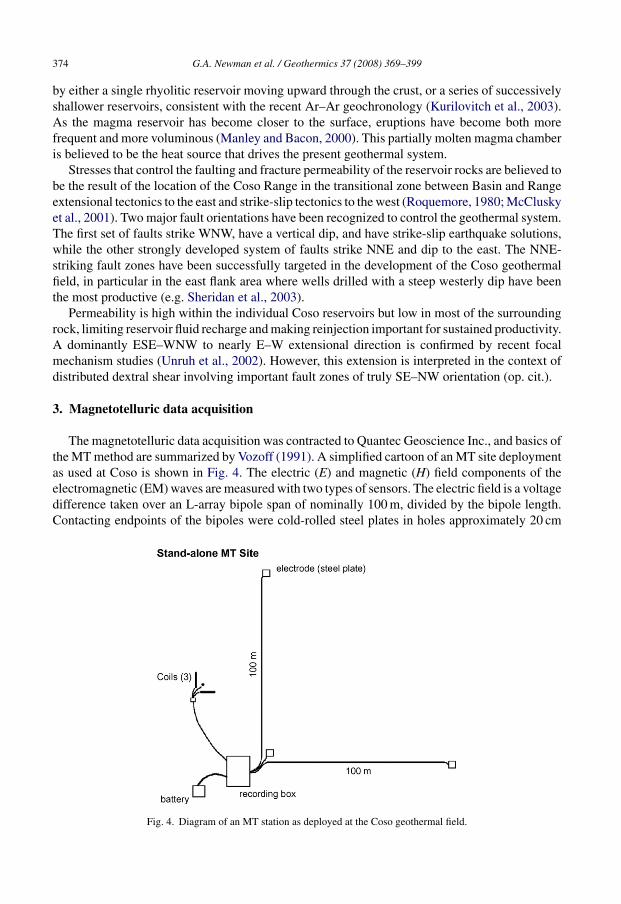
The magnetotelluric data acquisition was contracted to Quantec Geoscience Inc., and basics ofthe MT method are summarized by Vozoff (1991). A simplified cartoon of an MT site deploymentas used at Coso is shown in Fig. 4. The electric (E) and magnetic (H) field components of theelectromagnetic (EM) waves are measured with two types of sensors. The electric field is a voltagedifference taken over an L-array bipole span of nominally 100 m, divided by the bipole length.Contacting endpoints of the bipoles were cold-rolled steel plates in holes approximately 20 cm

Fig. 4. Diagram of an MT station as deployed at the Coso geothermal field.


deep with about one liter of water added to improve contact. The magnetic fields were obtainedusing high-sensitivity solenoids (coils) with built in preamplifiers, manufactured by EMI Inc.These were buried a similar depth for thermal and mechanical stability. Due to the remote natureof the sources and the high index of refraction of the earth relative to the air, the source fieldsare assumed to be planar and to propagate vertically downward. However, two axes of E andthree axes of H are measured because the scattering of EM waves by subsurface structure can bearbitrary in polarization, necessitating a tensor description.

Broadband EM times-series are recorded by these devices, and they are decomposed intoindividual frequency spectra through Fourier transformation. By way of band averaging andratios we arrive at the tensor impedance of the earth to vertically incident, planar electromagneticwave propagation; i.e. the fundamental MT quantity that is interpreted for geological structure.This is expressed as:

E = [Z]H

where Z is a two-rank tensor. Individual elements of the impedance are subject to simple arithmeticto obtain an apparent resistivity and impedance phase, which are more intuitive to inspect andinterpret (Vozoff, 1991). The nominal frequency range recorded was from 250 to 0.01 Hz, whichspans a depth range of several tens of meters to depths greater than 10 km. The assumption ofa planar geometry for the MT fields is crucial in the interpretation of the data and artificial EMsources nearby can invalidate it. An obvious source could be the high-voltage, 60 Hz electricalproduction in the field, which may be strong enough under transmission lines or next to generationplants as to saturate MT recording electronics. Strictly speaking, however, the loss of a very narrowband of results around 60 Hz is generally not serious since the impedances are a smoothly varyingfunction of frequency. More problematic are broadband noises whose causes are often obscure butcan include power system load fluctuations (either within the Coso field or from nearby interstatetransmission lines), rotating machinery, and vibration. These are especially onerous in the so-called MT “deadband”, a frequency band spanning 3–0.1 Hz, where the MT fields are particularlyweak and would correspond to 2–5 km depth at which the geothermal reservoir(s) may be located.

3.1. “Local” remote reference processing attempts

The remote reference method (Vozoff, 1991) is designed to overcome environmental noisethrough coherent detection utilizing simultaneous, remotely recording sensors that are completelyoutside the influence of the noise sources. The reference site of course may have its own noises,but as long as these are uncorrelated with the local site, the detection principle remains valid. Itis required that the remote site is of high fidelity or the final result will be degraded or a greaterlength of averaging time will be needed to achieve equivalent results (e.g. Egbert, 1997).

In the first Coso MT survey of 2003, reference sites were attempted at five locations of varyingdistance from the geothermal field (Wannamaker et al., 2004). The nearer three sites were theCentennial Flat area, Panamint Valley and Amargosa Valley, which are about 24, 48 and 100 kmfrom the Coso field, respectively (Fig. 5). Time series from these sites were downloaded to a fieldcomputer by the local Coso collection crew for processing at essentially the same time as thosein the Coso geothermal field, which is normal survey procedure. For the more distant referenceswe discuss later, more elaborate communications procedures were required.

The MT apparent resistivities corresponding to impedance elements Zxy and Zyx for the refer-ence site at Centennial Flat and in Panamint Valley are shown in Fig. 6. Characteristic of non-MTartificial effects are apparent resistivities which rise with decreasing frequency at an anomalously


Fig. 5. Location of “remote” MT references used in the Coso MT study: Centennial Flat (CEN), Panamint Valley (PAN),Amargosa Valley (AMG) and Parkfield (PKD). Not shown is Socorro, NM, some 1000 km to the east. Also shown arethe trace of the Bonnerville Power Authority (BPA) DC intertie transmission line (bold red line), which was provided byJim Lovekin, and the location of San Francisco (SF), Los Angeles (LA), Las Vegas (LV), and Carson City (CC).

steep rate in the weak MT middle band, and then fall almost discontinuously around 0.1 Hzwhere the MT fields become quite strong again due to solar wind energy. This is apparent atthe Centennial Flat site, as is the case for soundings generally in the Coso area processed usingthese references. These non-MT artificial effects are analogous to that seen in controlled-source(CSAMT) surveys when the transmitter is too close to the survey area (Zonge and Hughes, 1991;Wannamaker, 1997).

The distortion propagates to frequencies lower than 0.1 Hz to an unknown degree so thatstructural images in the pertinent depth range of several km may be unreliable. Essentially onlythe xy-component is affected in the Coso survey, which corresponds to an E-field directed N–S(x-direction). This behavior implicates the Bonneville Power Authority (BPA) DC intertie trans-mission line that runs in this direction nearby to the west of the Coso field (Fig. 5), and whichbroadcasts electric fields roughly parallel to itself. Similar broadband non-plane wave effects dueto interstate DC interties have been observed occasionally in other surveys (e.g. Wannamaker etal., 1997, 2002).

In an attempt to escape the influence of the DC intertie, remote references were tried also inPanamint Valley and Amargosa Valley, about 48 and 100 km distant from the intertie, respectively.The sounding from Panamint is shown in Fig. 6. This good-quality sounding does not show the


Fig. 6. (a) Apparent resistivity soundings taken at Centennial Flat about 24 km north of Coso. (b) Apparent resistivitysoundings taken in eastern Panamint Valley, about 48 km northeast of the field. Note the abrupt change in Rho-xy around0.1 Hz, indicative of a near-field (NF) or non-MT source field effect at Centennial Flat, and its absence at the more distantsite (Panamint Valley). These plots were provided by the contractor (Quantec Geoscience Inc.) before final processingand band-averaging to define inversion data.

cusp-like behavior near 0.1 Hz seen in Centennial Flat, and the site at Amargosa Valley was evencleaner. Initially, we concluded from this that influence of the DC intertie at these distances wasminimal and that the sites would constitute sufficient references. However, other soundings inthe Coso area processed using these references still showed significant cusp-like behavior in thisfrequency range (Fig. 7, site E13 taken ∼1/2 km east of well 34–9; see Fig. 1), although theresults using the more distant Amargosa site were better. This was disappointing as 100 km ofoften winding road was reaching the limit in terms of practical, on-site reference retrieval.

It is evident that a site giving good quality plane-wave (MT) results does not necessarily serveas a good remote reference for soundings taken in a noisy environment. Clearly, EM fields whichare correlated with the DC intertie are persisting at least as far away as the Amargosa Valley ref-erence. This is occurring even though such fields have become planar by this point and only serveto improve the local MT responses at Panamint and Amargosa Valleys (e.g. see Fig. 6). The pow-erline fields in the Coso field area, which are quite non-planar, remain correlated in time with thePanamint and Amargosa sites and thus are not removed by remote reference processing. As empha-sized by Wannamaker et al. (2004), a reference must be established which is completely outsidethe domain of the noise source in a survey, not just placed where the noise has become planar.


Fig. 7. Apparent resistivity data from MT Site E13 (Fig. 10) in the Coso geothermal field processed using Panamint Valley(upper) and in Amargosa Valley (lower) as remote references. Some near-field (NF) effect appears to remain near 0.1 Hz.

3.2. Distant remote references: Parkfield (California) observatory and Socorro (NewMexico)

More than 40 MT soundings had been taken at Coso using the various references describedbefore the far-reaching nature of the noise source was truly recognized. To obtain high-quality results at these locations, we were faced with a complete reoccupation using a yetmore distant reference, which would be expensive, or else locate a reference site of opportu-nity which fortuitously happened to be running while the Coso survey was underway. Sucha reference site in fact exists in the way of the Parkfield, CA (PKD), permanent MT obser-vatory, run by the University of California Berkeley Seismological Laboratory (for info, seehttp://www.ncedc.org/bdsn/em.overview.html) (Fig. 5). Due to power-law falloff and inductivedissipation of EM fields from a line-source, the DC intertie fields at PKD should be weaker thanthose at Amargosa by about a factor of 5, making the attempt to use PKD worthwhile. The EMtime series are available at no charge essentially in real time through an ftp request. They aresampled at a rate which allows their use as a reference for frequencies up to 14 Hz, which coversthe contaminated band at Coso. A plot of the results for MT Site 13 appears in Fig. 8 and indicatesthat the near-field effect has been corrected. The principal frequency range of distinction betweenthe Parkfield-processed and the previous results is 1–0.1 Hz. Similarly good results were obtainedfor reprocessing the other about 40 sites of the Coso area.

http://www.ncedc.org/bdsn/em.overview.html


Fig. 8. Apparent resistivity data from MT Site E13 (Fig. 10) in the Coso geothermal field processed using the ParkfieldMT observatory as a remote reference.

This outcome is very fortunate, but there was concern that Parkfield is barely adequate indistance and that during times of exceptionally low natural MT field activity or large powerlinefluctuations there still could be some soundings whose quality would be compromised. Hence,for the remaining MT Coso soundings taken in 2003, a remote reference near Socorro, NM(SOC), more than 1000 km to the east, was used. Because it is important to recognize surveyingproblems as they may occur, the Coso and the reference time series should be brought togetheras quickly as possible. To achieve this, the field crew at Coso uploaded acquired time series tothe University of Utah/EGI ftp site using the Caithness Energy high-speed computer facilities atCoso Junction, CA. The contractor’s data processor/reference operator in Socorro downloadedthese series from Utah using the high-speed computer facilities of the New Mexico Institute ofMining and Technology. The Coso site and reference time series thereby were combined severalhours after their acquisition.

To verify that the MT time series at Socorro are well correlated with those at Coso, and Park-field, we compare results from MT Site 29 processed with PKD with those processed using SOC(Fig. 9). The sounding curves are essentially identical indicating that Parkfield was an adequatereference in this case, although we view Socorro with more assurance as a quiet site outsidethe influence of the DC intertie. We considered the unusual effort of requiring the establish-ment of a quiet remote reference free from both local and broad-scale artificial EM interferencenecessary.

The fluid producing fractures at Coso are between 1 and 3 km depth (Adams et al., 2000) inplutonic rocks covered by a variable layer of hydrothermally altered overburden. This situationdetermines the first-order character of the soundings shown thus far, namely apparent resistivitiesin the 10–30 � m range for frequencies higher than 3–10 Hz rising to values near 100 � m at lowerfrequencies. Subtle variations in the upward slope of the apparent resistivity and the correspondingimpedance-phase responses provide the second-order evidence for bedrock structure of potentialgeothermal significance. Thus, high-quality MT soundings are required.

Unfortunately in the second data campaign of 2005, the contractor (Apollo/Phoenix Geo-physics) did not implement such a distant remote reference and the data were contaminatedsimilarly as in our first survey before action was taken to use distant remote reference sites (Park-field and Socorro). Nevertheless these data were judged to be of sufficient accuracy down to0.1 Hz that they could be included in a 3D MT interpretation of the Coso area; they are useful in


Fig. 9. (a) MT Site E29 sounding (Fig. 10) processed using the Parkfield observatory as a reference. (b) MT Site E29sounding processed using the Socorro site as a reference.

constraining the southern boundary of the geothermal field. Because these data are not as accu-rate as those acquired in the first phase of the measurements, we cannot expect to extract subtlevariations in the data to the same degree as with the 2003 information.

4. Magnetotelluric inversion

Our ultimate aim was to construct a 3D resistivity model of the Coso geothermal field and useit to better understand its hydrothermal system by correlating it with independent geological andother geophysical information. To accomplish this goal we applied an inversion process, where theobserved impedance data were fit in a least squares sense to the calculated data (i.e. the “model”).The computed data were produced by solving Maxwell’s equations for 3D resistivity variationsand plane-wave source excitation at a discrete set of frequencies, which correspond to those usedto specify the impedance tensor in the field measurements. To stabilize the inversion process,additional constraints were added such as spatial smoothing and bounds on the resistivity model.Because 3D MT inversion and modeling requires significant computational resources and time(Newman and Alumbaugh, 2000; Newman et al., 2003), it was more efficient to build the initial3D resistivity model from 2D imaged sections of the reservoir. This starting model was refinedsubsequently through the 3D inversion process.


Fig. 10. Map of the Coso MT survey area; elevations given in meters above sea level. Line NA1 is contiguous to thebipole profile Navy Array 1. Sites 1–102 were acquired in 2003, and Sites 103–125 in 2005. Observed and predictedimpedance data (apparent resistivity and phase) from the final 3D resistivity model will be compared along the obliquetransect (3D-PF) in Fig. 18. The transect uses MT Stations 99, 100, 88, 89, 71, 72, 65, 50, 41, 32, 22, 13 and 8. Lines L1,L4, and L8 indicate the location of three of the 2D profiles used for the 3D starting model (see Fig. 13).

4.1. Two-dimensional data interpretation

The initial 2D inversion was performed on relatively sparse E–W profiles of 8–10 MT sitesselected from the survey map shown in Fig. 10, utilizing the 2D MT inversion algorithm ofRodi and Mackie (2001). We did not use the 2005 data in this exercise because of noise problemsbelow 0.1 Hz due to the lack of a good remote reference. The inversions were carried out using Zyx

impedance data and analyzed assuming the electric field is polarized perpendicular to a presumedN–S geological strike (x-axis); in actuality, polar diagrams show that geological strike varies withfrequency (i.e. it is 3D), but at the lowest frequencies (<0.1 Hz), the polarization ellipses align ina NNE direction, which follows the trend of the Basin and Range fault-block geology. In spite ofthe obvious limitations in modeling and inverting the Coso data in 2D, it was a logical startingpoint for carrying out a full 3D analysis. Here the Zyx apparent resistivity and phase are definedas the transverse magnetic (TM) mode for use in the 2D inversion because 3D modeling showsthat it is usually more robust than the transverse electric (TE) data to non-2D effects such as finitestrike and static shifts (e.g. Wannamaker et al., 1984; Wannamaker, 1999).

Shown in Figs. 11 and 12 are 2D fits to Coso resistivity and phase data along the profile contain-ing MT Sites 45 through 53 (L4 in Fig. 13). Fits to the apparent resistivity data (red curves) agree


Fig. 11. Two-dimensional TM fits to the Zyx apparent resistivity data, where open circles represent the field data and redcurves the model responses. See Fig. 10 for site locations.

Fig. 12. Two-dimensional TM fits to the Zyx impedance phase data, where open circles represent field data and red curvesare model responses. See Fig. 10 for site locations.


Fig. 13. Starting resistivity model of the Coso geothermal site compiled from multiple 2D transects (location of transectsL1, L4 and L8 are given in Fig. 10). Traces of wells 64-16RD, 22-16ST and 34A-9 are also shown. Elevations (Z) aregiven in meters above sea level.

closely with the field observations over the entire frequency band. The phase data, however, donot fit as well, especially below 0.1 Hz, most likely indicating a 3D characteristic of the data. Theresulting 2D (vertical) resistivity distribution for this profile, as well as those from others, is pre-sented in Fig. 13. Perhaps the most conspicuous feature of our ensemble of 2D inversion sections isa moderate low-resistivity zone dipping steeply west from the Coso east flank area; between Nor-thing 79,000 and 77,000 m; this zone terminates abruptly both to the south and the north. Severalof the more productive wells on the east flank dip toward this structure suggesting some correlationwith higher permeability and fluid content. Wannamaker (2004) first identified this conspicuousfeature using 2D TM mode analysis of the dense array Line NA1 shown on Fig. 10. The 2D inver-sion model of this line (Fig. 14) provides more details than individual sections of the 3D resistivitymodel due to the contiguous sampling over 52 bipoles, each 100 m in length. The inversion ofLine NA1 also shows the west dipping lower resistivity zone seen in the sections of Fig. 13.

Fig. 14. Two-dimensional resistivity inversion model using TM mode data of contiguous bipole profile NA1. Also plottedare the traces of deep wells 34-9RD2 and 34-A9 that project from about 500 m south of the profile. The bottom of 34-9RD2corresponds to a lost circulation zone. The inversion code used is based on the forward problem of Wannamaker et al.(1987) and model sensitivities of de Lugao and Wannamaker (1996).


Production well 34-9RD2 grazes the eastern boundary of this lower resistivity zone (Fig. 14).Over the bottom 350 m of the well, where it approaches the conductor most closely, a very largelost circulation zone was encountered indicating an interval with substantial open porosity (PeterRose, personal communication, December 2006). Shallow low-resistivity material in the modelrepresents thin alluvium and clay alteration over the eastern flank of Coso, and deeper alluviumat Coso Wash, toward the eastern part of the modeled section. Wannamaker (2004) noted that itwas necessary to consider a 3D interpretational framework to fully explain all the data, not justselected modes of the data identified as TM and TE from the 2D analysis.

4.2. Three-dimensional inversion of the Coso field data

The massively parallel algorithm described by Newman and Alumbaugh (2000) was used forthe 3D modeling and inversion of the Coso field data, where eight 2D TM mode inversions shownin Fig. 13 were spatially interpolated to form the core of a 3D model beneath the data acquisitionsites. This core model was then extended laterally over 100 km and to nearly 100 km in depth. Thelarge area around the core model is required to satisfy the boundary conditions (scattered fields areassumed to be zero on the boundary) of the finite-difference (FD) model. The resulting 3D finitedifference grid used to simulate data arising from the model, employed 244 by 258 by 120 nodesin the x, y and z directions, respectively. The FD cells were 100-m sided cubes within the centralportion of the mesh defined by the data acquisition sites. Away from the site locations the meshcells grew in size as they approached the outer boundaries. The maximum cell dimension aspectratio was 8 to 1, so that no dimension of a boundary cell was greater than 800 m. The interpolated3D resistivity model provided the starting model for the 3D inversion. The simulated fields (Zxy

and Zyx apparent resistivity and phase) for this starting model are shown in Figs. 15 and 16 andare compared with the corresponding field observations for Sites 45 through 53.

For frequencies above 1 Hz, the 3D fields generally show good correspondence with the mea-sured data for both polarizations, even though there are some grid-induced statics arising from theinterpolation process that affect primarily the predicted Zxy apparent resistivity at a few sites. Itis expected that the Zxy data would show the poorest fit to the 3D model because it is constructedof 2D sections generated by fitting the Zyx data. Significant differences, however, arise at all sitesbetween the model and field curves in both apparent resistivity and phase at lower frequencies.When the field data were analyzed using 2D assumptions, such discrepancies were most apparentin the phase data.

While all the complex impedance tensor elements can be considered as data in the inversion,it was found that the on-diagonal terms (Zxx, Zyy), which have much lower magnitude, and thuslower signal-to-noise, than the off-diagonal terms (Zxy, Zyx), generally degraded the performanceof the inversion. Thus, we included only the off-diagonal elements. Also designing a FD meshthat will accurately represent the electromagnetic fields over the entire frequency range in theinversion of the observed data can be quite challenging. Practical considerations required that theentire frequency range of the data was not to be fitted simultaneously at first, but in three phases.

In the solutions presented here we first restricted the 2003 data over the 250–1 Hz frequencyrange utilizing a mesh with 120 nodes along each coordinate direction that spanned distances of120 km in the horizontal dimensions to satisfy boundary conditions. The mesh also extended 30 kminto the air and 60 km into the Earth. The smaller mesh utilized for this frequency range allowedfor fast processing times and the model obtained was used as a starting model in the next phaseof the image processing. In the second phase we added 2003 data down to 0.3 Hz, and in the finaland third phase we added the data acquired in the 2005 campaign (250–0.3 Hz). To accommodate


Fig. 15. Comparison of apparent resistivities for Sites 45–53 that were based on the initial 3D starting model generatedfrom the interpolated 2D TM mode inversion. The blue curves with solid and open squares denote predicted and observedZxy apparent resistivities, respectively. The red curves, solid and open circles, denote predicted and observed Zyx apparentresistivities, respectively.

Fig. 16. Comparison of impedance phases for Sites 45–53 that were based on the initial 3D starting model generated fromthe interpolated 2D TM mode inversion The blue curves with solid and open squares denote predicted and observed Zxy

phases, respectively. The red curves, solid and open circles, denote predicted and observed Zyx phases, respectively.


Fig. 17. Plot of the convergence of the 3D inversion iteration for the 100–1 Hz data. The dashed curve is a plot of theconvergence of the error functional with the regularization constraint. The solid curve is a plot of the data mistfit (weightedsquared error) without the regularization penalty term.

the lower frequency data in phase two and three of the image processing, we expanded the meshto 244, 258 and 120 nodes along each coordinate in order to move its boundaries out a sufficientdistant to insure quality results. The accuracy of these two meshes were tested and verified towithin a few percent based on 1D forward models over the two frequency ranges, and were shownto have depth sensitivity to 5 and 15 km, respectively. This should be adequate for mapping thedepths of interest in the geothermal system.

Out of the 102 MT stations acquired in 2003 over the east flank of the Coso field, only one stationwas discarded because of severe noise problems; we also disregarded data from six stations of the2005 survey. In the inversion processing we assumed a 5% noise floor, based upon the amplitudeof each impedance measurement, where the data were weighted by the noise estimates.

The first 3D inversion analysis (250–1 Hz data) was carried out at the National Energy ResearchScientific Computing Center (NERSC) of Lawrence Berkeley National Laboratory, where 512IBM SP2 processors were employed. On this platform for a 48-h period, 15 inversion iterationscould be completed on average. Shown in Fig. 17, is a plot of the convergence of the inversion iter-ation. The dashed curve is a plot of the convergence of the error functional with the regularizationconstraint. The step-like features in this graph correspond to reducing the level of smoothing inthe inversion process as the iteration proceeded. The solid curve is a plot of the weighted squarederror, the data misfit without regularization. While we did not achieve the target data misfit of one,we observed a good reduction in the weighted squared error from 149 to 4.8 at the 88th inversioniteration.

Subsequent analysis using the lower frequency data was carried out on a more powerful Infini-band Linux cluster utilizing 100 processors; for the same number of processors the Linux clusteris about 3–5 times faster than the NERSC platform. With the 2003 augmented data we were able


Fig. 18. Pseudo-section plots of Zyx and Zxy apparent resistivities and phases for observed and predicted data along thetransect 3D-PF indicated in Fig. 10. The predicted data arise from the final 3D resistivity model given in Fig. 19. Horizontaloffsets in these plots are relative to Site 99. Predicted results are shown for the first and final inversion iterations showingthe improvement obtained in the data fit.

to reduce the data misfit to 2.99, which is still a factor of three above the desired noise threshold.When we added the 2005 data the final misfit was 3.2. Closer inspection of the data fits indicatesthe inability to fit the data to the assumed noise threshold appears to arise from noise in the MT3–0.3 Hz deadband, which also appears to affect the 2005 data more than those of the 2003 cam-paign; this should come as no surprise given the use of a “local” remote reference in the 2005survey. Nevertheless the predicted data produced from the resistivity model based on both the2003 and 2005 data sets showed good improvement when compared to those generated by thestarting model (Fig. 18).

4.3. The three-dimensional resistivity model

The final 3D resistivity inversion model is illustrated in Fig. 19. The most obvious featureis the red core of low resistivity centered within well production and reinjection intervals alongwith micro-earthquake (MEQ) locations. Most of the MEQ events are related to volumes changesarising from commercial exploitation of the reservoir (Julian et al., 2004). The event locationsalso appear to correlate with transition boundaries in the resistivity to some degree; we will havemore to say about this later.

A horizontal depth slice from the final model at an elevation of 500 m below sea level inFig. 19 is given in Fig. 20. The most prominent feature in this figure is the low-resistivity centralregion. The mapped surface expressions of right-lateral faults running S–N in the figure bound this


Fig. 19. Three-dimensional 3D resistivity image derived from Coso MT data sets. Black and red linear segments denotewell production and reinjection intervals. The red dots correspond to micro-earthquake focus locations. Elevations givenin meters above sea level.

region to the NE and SW, implying the faulting is nearly vertical to 1000 m depth. This region alsoexhibits temperatures above 250 ◦C, high permeability and contains large amount of fluids. Onthe other hand, the area around MT Sites 87, 88, 98, 99, and 100 has similarly high temperaturesand significant geothermal fluid production from 2 to 3 km depth, but shows only moderate, anda non-descriptive resistivity structure of approximately 50 � m; we shall discuss the implicationsof this finding in more detail later on. This zone is also clearly bounded by NE–SW and NW–SEtrending faults that define the productive area of the field and appear to act as hydrologicalbarriers.

Because the low-resistivity structure is such a conspicuous feature in the 3D resistivity model,which persists from the prior starting model, a sensitivity test was carried out where the structurewas replaced by the more resistive material on its flanks. The resulting data misfit was 35% greaterthan what was observed for the final misfit with the low-resistivity structure, indicating its impor-tance in the model. Furthermore, two other independent observations confirm this assessment.As we already mentioned, fault traces in Fig. 20 clearly mark the NE and SW boundaries of thestructure. More convincingly we shall present below the 3D seismic velocity model of Coso ofLees and Wu (2000) developed based on MEQ data that shows a stunning correlation with thelow-resistivity structure in Fig. 20.

A vertical (W–E) section at Northing 81,000 m (PF1 in Fig. 20) is given in Fig. 21. In theeastern part of this section, the resistivity structures dip to the east and implies that in this area thethickness of the sediments in the Coso Wash graben is less than about 1000 m. The two unnamednormal faults depicted in Fig. 20 as “2” and “3” and the Coso Wash fault “1” correlate with theeasterly dipping resistivity structures; the sediment thickness in the downthrown blocks of thesefaults increase to about 2000 m. To the west, subvertical contacts between low- and high-resistivitymaterials are evident.

Fig. 22 shows a vertical (W–E) section at Northing 79,900 m that intersects the Coso HotSprings (PF2 in Fig. 20), which are located directly above a high-resistivity feature on the easterlydipping contact between the central resistor and the more conductive valley fill to the east. Notethat the area around and north of Coso Hot Springs is a protected historical site; hence no drillingis allowed in this part of the geothermal field.


Fig. 20. Horizontal slice through the 3D resistivity model at 500 m below sea level; average ground surface elevation is1200 m above sea level. Geothermal surface manifestations areas are outlined in white. Mapped surface fault expressionsare shown by the brown lines (dotted were inferred); (1) correspond to the Coso Wash Fault, while (2) and (3) to twounnamed faults. Micro-earthquake seismic stations (S1, S2, S3, S4, S5, S6, S7 and N1) from Lees and Wu (2000) areshow in purple. MT sites are indicated by the black crosses. White dashed lines (PF1, PF2, NA1, PF3, PF5 and PF4)correspond to the location of the vertical cross-sections of the final model shown in Figs. 21–25 and 27, respectively.

Fig. 23a is a vertical section corresponding to the 2D resistivity section along the high-densityMT line of Wannamaker (2004) (NA1 in Fig. 20) shown in Fig. 14. The vertical section throughthe 3D model at a location 700 m to the south is shown in Fig. 23b for comparison. The 2Dinversion in Fig. 14 appears to be responding to the resistivity structure given in Fig. 23b. Inother words, the vertical section in Fig. 23b is much closer to the 2D inverted result than is thesection directly beneath the 2D line. The 2D and 3D inversion sections to first-order imply thatthe dipping conductor becomes much more pronounced to the south of the dense array line (LineNA1).

The 3D inversion sections overall are expected to be a more accurate representation of structuredirectly beneath them since an attempt was made to fit both impedance polarizations of all profiles,simultaneously. However, we do not believe the conductor imaged under Line NA1 is entirelydue to sideswipe from the lower resistivity found 500 m or more to the south. This is because the2D image in Fig. 14 is only 200–300 m wide where it comes near the surface. We conclude theremust be a vestige of the dipping conductor under or very close to Line NA1, but the advantageof 3D coverage is that the maximal expression of the conductor can be pinpointed with moreconfidence.


Fig. 21. Vertical (west to east) resistivity cross-section PF1 at Northing 81,000 m. The fault marked (1) is the Coso WashFault, faults (2) and (3) are unnamed and shown in plan view in Fig. 20. The horizontal black dashed line corresponds tothe elevation of the horizontal slice shown in Fig. 20. The resistivity in the air region was set at 1010 � m, but is indicatedat the top of the section by a dark blue strip (103 � m) on the color scale to compress the resistivity range and better renderthe resistivity variations within the Earth.

An S–N transect (PF3 in Fig. 20) that intersects the Devil’s Kitchen structure is shown inFig. 24. As with the resistivity structure beneath the Coso Hot Springs, Devil’s Kitchen is over ahigh-resistivity feature at depth. Its location coincides with the surface termination of a high–low-resistivity contact that would suggest a fault that in Fig. 24 dips to the north from Devils’ Kitchen.

Fig. 22. Vertical (west to east) resistivity cross-section PF2 at Northing 79,900 m. The section intersects Coso Hot Springsat the location shown by white arrow. The horizontal black dashed line corresponds to the elevation of the horizontal sliceshown in Fig. 20. The resistivity in the air region was set at 1010 � m, but is indicated at the top of the section by a darkblue strip (103 � m); see caption of Fig. 21.


Fig. 23. (a) Vertical (west to east) resistivity cross-section at Northing 79,100 m which is the location of the high-densityMT line (Line NA1) used to generate the 2D resistivity section shown in Fig. 14. (b) Vertical (west to east) cross-section atNorthing 78,400 m. The horizontal black dashed lines correspond to the elevation of the horizontal slice shown in Fig. 20.The resistivity in the air region was set at 1010 � m, but is indicated at the top of the section by a dark blue strip (103 � m);see caption of Fig. 21.

This is an area exhibiting subsurface temperatures above 250 ◦C and crustal thinning that exem-plifies the Coso reservoir as a whole (Monastero et al., 2005), where the brittle–ductile transitionzone is at about 4 km depth.

High resistivity in the Devils’ Kitchen area corresponds with many of the production wellintervals and is interpreted as a resistive propylitic alteration zone within the reservoir; we willhave more to say about this shortly. There are two low-resistivity zones—a shallow one thathas lateral continuity, and a deeper one that is possibly related to the brittle–ductile transition.The PF3 transect also intersects an area of high geothermal well density, where the near sur-face low resistivity is interpreted as a clay cap alteration zone caused by the geothermal fluidsbeneath.


Fig. 24. Vertical (south to north) resistivity section PF3 at Easting 717,900 m that runs through the Devil’s Kitchenarea. Black and red lines indicate producing and injection well intervals, respectively. The horizontal black dashed linecorresponds to the elevation of the horizontal slice shown in Fig. 20. The resistivity in the air region was set at 1010 � m,but is indicated at the top of the section by a dark blue strip (103 � m); see caption of Fig. 21.

The producing intervals of all the wells between Easting 717,400 and 717,900 m are shown asnearly vertical black lines in Fig. 24; a single injection interval is shown as a red vertical line. Thisfigure illustrates two general observations about the correlation between well production zones andthe resistivity structure, (1) to the north of Northing 76,000 m the producing intervals are located inhigh-resistivity material below the low- and high-resistivity transition zone, and (2) in the SW areaof our survey (south of Northing 76,000 m) there is an area of intermediate resistivity (∼50 � m)with no sharp resistivity contrasts where many successful production intervals are found.

The perpendicular transect at Northing 76,000 m through the SW area of our survey (PF5 inFig. 20) is presented in Fig. 25. Here again a conductive cap is observed overlying the more resistivereservoir rocks; it has already been illustrated that fluid production in the southwest sector of theCoso field appears to be controlled by the fault geometry shown in Fig. 20. Further observationalong the Devil’s Kitchen transect (Fig. 24) suggests that the deformation caused by igneousintrusions has produced significant fracturing. The boundaries between the older and youngerrocks are represented by the transitions between low- and high-resistivity regions. We believe thefracturing at the boundaries provides good permeability for geothermal fluid production.

The images in Figs. 22 and 24 show a well-established pattern when MT is used to map geother-mal resources in high-temperature (>230 ◦C) environments, which is clearly the case at Coso. Theconceptual model consists of a conductive argillic (smectite clay) hydrothermal alteration zoneabove and adjacent to more resistive illite clays that formed from propylitic alteration within thegeothermal reservoir (Anderson et al., 2000; Cumming et al., 2000; Ussher et al., 2000); matrixconductivity within the reservoir is influenced much more by the resistive illite clays, than thefluid-filled fractures.

Lutz et al. (1996) has documented the clay mineralogy at Coso along the Devil’s Kitchentransect (Fig. 24), which varies systematically with temperature and depth. Three hydrothermalalteration zones were recognized: the smectite, illite–smectite and illite zones. The smectite andmixed smectite–illite zones were reported to thicken from north to south. The illite zone, thedeepest one, contains illite, chlorite, epidote and wairakite. These authors also reported that thedepth of illite zone increased from 750 m depth from the surface, in the vicinity of the Devil’sKitchen area, to depths greater than 1200 m to the south. This is consistent with the depth whereincreased resistivity is observed and corresponds to the shallowest part of the producing inter-


Fig. 25. Vertical (west to east) resistivity cross-section PF5 at Northing 76,000 m. This section intersects a region with alarge number of geothermal well feed zones between Easting 717,400 and 719,000 m. The horizontal black dashed linecorresponds to the elevation of the horizontal slice shown in Fig. 20. The resistivity in the air region was set at 1010 � m,but is indicated at the top of the section by a dark blue strip (103 � m); see caption of Fig. 21.

vals in Fig. 24. The temperature observed with this change in clay mineralogy corresponds toapproximately 230 ◦C.

The shape of the subsurface resistivity structure in Figs. 22 and 24, best exemplifies the anomalyof choice for delineating high-temperature geothermal reservoirs; a conductive clay cap diagnosticof the underlying reservoir that also shows an apex in the base of the argillic–smectite clay capbeneath a fumarole area (e.g. Coso Hot Springs and Devil’s Kitchen). A case could be made inapplying this conceptual model to the resistivity section in Figs. 21 and 23a, and Fig. 25 as well,but the resistivity section in Fig. 23b is too complex to be easily described by this model.

4.4. The geophysical signature

Electrical resistivity and seismic velocity depend on many physical conditions. Within thecomplexity of a geothermal system it is difficult to isolate unique relationships that allow an unam-biguous interpretation of inferred geophysical parameters such as electrical resistivity, acousticand shear velocity. Just as the physical properties, mineral composition, fracturing, fluid satura-tion, temperature, porosity and pressure, affect the geothermal characteristics of the subsurface,they also influence the geophysical parameters that can be inferred from the surface. In this studywe investigated first-order correlations between seismic and electrical geophysical structure andsuggest causative mechanisms for anomalous regions.

Electrical resistivity is primarily a function of water/brine saturation, porosity and the electricalresistivity of the fluid filling the pore space (Palacky, 1987). In fractured media, porosity andpermeability are dominated by that of the fractures. The electrical resistivity of the pore water iscontrolled mainly by salinity and less so by temperature. The mineral composition of the rocks,particularly the amount and type of clays present, also has a first-order effect on the bulk electricalresistivity of the rock mass.


For rock of relatively uniform composition both acoustic and shear velocity decrease withincreasing temperature (Christensen, 1989). Acoustic velocity (Vp) tends to decrease faster withtemperature than shear velocity (Vs) resulting in a decrease in the Vp/Vs ratio as temperatureincreases. However, the situation is more complicated in the Earth, where Vp/Vs ratio is observedto increase with temperature and fracture density (Sanders et al., 1995). Rocks with randomlyoriented fractures have smaller seismic velocities compared to those of unfractured rocks. SinceVp decreases less than Vs as the density of fractures increases, generally Vp/Vs is higher whenrock fracture density is greater (Schon, 1996). Acoustic velocity generally increases with fluidsaturation, while shear velocity is only slightly affected by the change in density.

4.5. The MT resistivity and MEQ velocity models and their interpretation

A synthesis of much of the previous geochemical and geophysical work at Coso is given by Leesand Wu (2000). They present an intrusive model for Coso that places a magmatic body at depthsgreater than 5 km below the triangle formed by micro-earthquake (MEQ) Stations S1–S3–S4 andpropose the following model. The center of magma movement is close to the S1–S3–S4 triangle(just to the SW of our MT survey area shown in Fig. 26). Hot magma arose from depth and spreadout in all directions. It flowed due north and east following the two pre-existing sets of faults.

The 3D seismic velocity model derived from tomographic inversion of MEQ data (Wu andLees, 1999; Lees and Wu, 2000) was provided to us for comparison with the 3D MT resistivitymodel. The tomographic model used a cell size of 200 m by 500 m in the horizontal and verticaldirections, respectively. The MEQ inversions produced models of acoustic and shear velocities,and the associated Vp/Vs ratios.

Examination of the 3D velocity and 3D resistivity models shows many interesting correlations.Fig. 26 depicts the Vp/Vs distribution at 500 m below sea level and the same surface features andmarkers used in Fig. 20. Black dashed lines indicate locations of vertical cross-sections PF1–PF5and NA1. The correlation between the high Vp/Vs and low resistivity in the central portion ofthe two figures (between Easting 718,500 and 720,500 m, and Northing 77,000 and 78,500 m) isstriking. The high Vp/Vs and low electrical resistivity region is bounded by two sets of mappedfaults. The area of low Vp and Vs, and high Vp/Vs, is interpreted by Lees and Wu (2000) asprobably being fluid-saturated. This is consistent with low electrical resistivity. Besides fracturedensity, Sanders et al. (1995) also point out that increases in Vp/Vs ratio are related to increases intemperature and partial melt. While at Coso there is no partial melt at reservoir depths, the reportedhigh temperatures (exceeding 250 ◦C) in this area may further enhance the Vp/Vs ratio. To the norththe low Vp/Vs and high resisitivity both align with the surface expression of the Coso Wash Fault.

In the southwestern corner of the MT survey (MT Stations 87, 88, 96, 99 and 100), whereone finds the anomalous ring structure in the Vp/Vs ratio (Fig. 26) and the intermediate electricalresisitivity on the order of 50 � m (Fig. 20), there is significant geothermal fluid production from2–3 km depth. Whereas the Vp/Vs ratio map provides a clear indication of production intervalsin the SW portion of the survey area, the electrical resistivity gives only a slight indication. Thislack of correlation between the Vp/Vs and resistivity structure in this region may be attributed tothe truncation of the MT survey data and/or its lack of sensitivity to the producing fluid intervals.We have no data to the south and west of the SW corner area and believe that better correlationscould be obtained if the MT data could be acquired there. Northeast of that corner we find aNW-trending band of high electrical resistivity and low Vp/Vs ratio.

North and east of Devil’s Kitchen there is a SW-trending zone of low Vp/Vs and high electricalresistivity that generally aligns with the surface expression of the Coso Wash Fault. This feature


Fig. 26. Horizontal slice through the 3D seismic velocity model derived by Lees and Wu (2000) on the basis of micro-earthquake (MEQ) data at 500 m below sea level; average ground surface elevation is 1200 m above sea level. Geothermalsurface manifestations areas are outlined in black. MEQ seismometer locations (S1, S2, S3, S4, S5, S6, S7, S8 and N1) usedfor velocity tomography are indicated in purple. Mapped surface fault expressions are shown by the brown lines (dottedwere inferred). Black dashed lines (PF1, PF2, PF3, PF4, PF5 and NA1) correspond to the locations of the cross-sectionspresented in Figs. 21–25 and 27.

is seen in the center of Fig. 21 with nearly vertical boundaries between low- and high-resistivityareas to the west and an easterly dipping contacts to the east.

There is a distinct difference between the SW area in Figs. 20 and 26 where high Vp/Vs correlateswith moderate electrical resistivity (∼50 � m) and the area to the NE (MT Stations 63, 64, 70,71, 72, 80, 81, 82 and 91) where high Vp/Vs correlates with low electrical resistivity (∼0.75 � m).Recent wells on the eastern flank of this latter structure that were drilled into the transition zonebetween the low- and high-resistivity regions encountered large open fractures that resulted inlarge drilling mud losses (Fig. 27) (Frank Monastero, personal communication, December 2005)indicating that there the formation fluids were under-pressured. The presence of these fracturesalong the flanks of the low-resistivity region, plus the high Vp/Vs feature suggests that this is an areathat is highly fractured and that fluids are nearby. Another intriguing possibility, given the reportedhigh temperatures in and around this structure, is that the low resistivity could have arisen fromthe boiling of formation fluids, where the remnant fluid exhibits increased salinities. However,fluids encountered in and around this area so far do not show any enhanced salinity comparedto fluids drawn from the western part of the field (Frank Monastero, personal communication,December 2007). Finally, it is important to note that the depth to the brittle–ductile transition


Fig. 27. Vertical (west to east) resistivity cross-section PF4 at Northing 77,900 m. The locations of zones major drillingmud losses (i.e. large open fractures) are shown by the black solid diamonds. All mud-loss locations are within 800 mto the north of the section and are in the transition zone between high- and low-resistivity regions. The horizontal blackdashed line corresponds to the elevation of the horizontal slice shown in Fig. 20. The resistivity in the air region was setat 1010 � m, but is indicated at the top of the section by a dark blue strip (103 � m); see caption of Fig. 21.

zone is shallowest here (i.e. at 3.5 km depth) and the area exhibits maximum crustal thinning(Monastero et al., 2005).

5. Conclusions

High-quality broadband MT data were acquired in the Coso geothermal field following effortsto establish an adequately distant, clean remote reference. It is not sufficient to use a referencesite that appears to give good plane-wave results local to the reference. This is because there maybe EM noise fields (albeit planar) at the reference site that are correlated in time with those ofthe survey area, which are non-planar in geometry. In the 2003 survey, we found that MT timeseries at the permanent Parkfield observatory in California were adequate as reference fields to thesites at Coso. In the course of doing this, technology has been established to generally utilize theParkfield data in MT surveying, thereby improving survey quality for other applications. Noisesources of scales as broad as that of the BPA DC intertie are rare, but this particular one may be afactor in exploration of numerous other geothermal systems in western Nevada and easternmostCalifornia due to its proximity.

A 3D resistivity model of the Coso geothermal field was developed using full 3D inversionof 125 MT sites over a frequency band of 250–0.3 Hz. In order to produce a geologically mean-ingful results the starting model was constructed from a series of 2D resistivity images alongE–W transects, approximately perpendicular to the regional geological strike. The 2D inversionswere carried out using Zyx impedance data and analyzed assuming the electric field is polarizedperpendicular to a presumed N–S geological strike. We employed this strategy to save time anda good starting model that could be better refined in the inversion process. The 3D resistivitymodel that was developed clearly confirms that faulting strongly controls the geological struc-ture, as well as geothermal fluid production at Coso. These faults act as hydrological barriers to


fluid flow, compartmentalizing zones where fluids can be exploited, and in some instances havebeen targeted by drilling into them from the east flank of the field. Several transects though the3D resistivity model show the classic MT response of a high-temperature geothermal reservoir,exemplified by Coso, which presents a conductive argillic (smectite clay) hydrothermal alterationzone that sits above and adjacent to more resistive propylitic alteration (i.e. illite clays) in thereservoir. Moreover, the conductive clay cap also shows at its apex diagnostic fumarole areas(Coso Hot Springs and Devil’s Kitchen).

Nevertheless there are limitations to this model. A key feature in the 3D resistivity modelpresented here that does not fit is the low-resistivity intrusive feature, confirmed by independentobservations. Based on drilling, this area is highly fractured and very hot (> 250 ◦C). Its lowresistivity cannot be ascribed to conductive clays because of the temperature. We surmise that thelow resistivity arises from large sets of fractures with fluids present in the vicinity.

A goal not yet achieved with this work was to conclusively show that 3D MT resistivity imagingcould provide sufficient information to map and directly identify fractures containing geothermalfluids that could be drilled into. On a larger scale, however, the 3D model has detected some ofthe controlling features that influence location of subsurface fluids and well production, notablyon the boundaries (faults) between mapped resistivity structures.

Another issue that could not be adequately addressed in this work is the problem of modelequivalence (non-uniqueness), which continues to be a serious issue in the interpretation of MTdata, especially in three dimensions. Without recourse to a good starting model, a 3D imagingexperiment may not provide value added information. Many factors determine the quality of animage, including not only the starting model, but the type of noise in the data, the frequencyband employed, spatial coverage and the robustness of the imaging algorithm. No doubt 3D MTimaging is and will be an ongoing research topic for years to come.

From the Coso experiment, we conclude that removal of static shifts in the data was veryeffective within the 3D inversion process, but activation of the deeper parts of the model space,below one km depth proved difficult without recourse to a good starting model. We believe thereare ways to remedy this shortcoming by incorporating lower frequency data within the inversionprocess at the expense of larger grids and greater computational costs. Use of more effectivedepth-weighting schemes and preconditioning the inversion iteration may also be helpful andwill be a subject of future studies. Nevertheless the focus of the current work is on an integratedinterpretation of the Coso MT measurements and correlations with independent geophysical datasets, as well as geological and well information. We believe the major correlations found thus farare convincing enough and provide a level of confidence in the 3D resistivity model developedfor the Coso system.

Acknowledgements

Data collection and processing were supported under U.S. Department of Energy Contract DE-PS07-00ID1391 and U.S. Department of the Navy Contract N68936-03-P-0303 to the Energy andGeoscience Institute. We thank Coso Operating Company for access to the field and to the high-speed Internet services that made the ultra-distant remote referencing possible. Similarly we aregrateful to New Mexico Institute of Mining and Technology (Prof. Harold Tobin) for providing aquiet reference site and fast ftp access. We also thank Frank Monastero, Steven Bjornstad and AllanKatzenstein of the U.S. Navy Geothermal Program office for support and encouragement, and forfunding all archeological site clearances. Finally, the competence and diligence of the field crew ofQuantec Geoscience, principally Jon Powell, Joel Cross, Claudia Moraga, Bill Doerner and Ken


Nurse, made results of this quality possible. Valuable discussions on MT data processing and useof the Parkfield facility were held with Gary Egbert (Oregon State University). The authors alsothank Jeff Unruh for permission to present Figs. 2 and 3 in this paper, and the comprehensive reviewand editing of the paper by Marcelo Lippmann. The data interpretation carried out at LawrenceBerkeley National Laboratory was supported with funding provided by the U.S. Department ofEnergy Geothermal Program Office under Contract No. DE-AC02-05CH11231 with additionalfunding provided by the U.S. Department of the Navy contract N69218-05-P-00101.

References

Adams, M.C., Moore, J.N., Bjornstad, S., Norman, D.I., 2000. Geologic history of the Coso geothermal system. GeothermalResources Council Transactions 24, 205–209.

Anderson, E., Crosby, D., Ussher, G., 2000. Bulls-Eye!—simple resistivity imaging to reliably locate the geothermalreservoir. In: Proceedings of the 2000 World Geothermal Congress, Kyushu–Tohoku, Japan, May 28–June 10, pp.909–914.

Christensen, N.I., 1989. Seismic velocities. In: Carmichael, R.S. (Ed.), Practical Handbook of Physical Properties ofRocks and Minerals. CRC Press, Boca Raton, FL, USA, pp. 429–546.

Cumming, W., Nordquest, G., Astra, D., 2000. Geophysical exploration for geothermal resources: an application for com-bined MT-TDEM. In: Society of Exploration Geophysicists Annual Meeting Technical Program Expanded Abstracts,6–11 August, Calgary, Canada, pp. 1071–1074.

de Lugao, P.P., Wannamaker, P.E., 1996. Calculating the two-dimensional magnetotelluric Jacobian in finite elementsusing reciprocity. Geophysical Journal International 127, 806–810.

Dixson, T.H., Miller, M., Farina, F., Wang, H., Johnson, D., 2000. Present-day motion of the Sierra Nevada block andsome tectonic implications for the Basin and Range province, North American Cordillera. Tectonics 19, 1–24.

Egbert, G.D., 1997. Robust multiple station magnetotelluric data processing. Geophysical Journal International 130,475–496.

Garg, S.K., Pritchett, J.W., Wannamaker, P.E., Combs, J., 2007. Characterization of geothermal reservoirs with electricalsurveys: Beowawe geothermal field. Geothermics 36, 487–517.

Julian, B.R., Foulger, G.R., Richards-Dinger, K., 2004. The Coso geothermal area: a laboratory for advanced MEQ studiesfor geothermal monitoring. GRC Transactions 28, 403–405.

Kurilovitch, L., Norman, D., Heizler, M., Moore, J., McCulloch, J., 2003. 40Ar/39Ar thermal history of the Coso geother-mal field. In: Proceedings of the Twenty-Eighth Workshop on Geothermal Reservoir Engineering, Stanford University,pp. 110–116.

Lees, J.M., Wu, H., 2000. Poisson’s ratio and porosity at Coso geothermal area, California. Journal of Volcanology andGeothermal Research 95, 157–173.

Lutz, S.J., Moore, J.N., Copp, J.F., 1996. Integrated mineralogical and fluid inclusion study of the Coso geothermalsystem, California. In: Proceedings of the Twenty-First Workshop on Geothermal Reservoir Engineering, StanfordUniversity, pp. 187–194.

Manley, C.R., Bacon, C.R., 2000. Rhyolite thermobarometry and the shallowing of the magma reservoir, Coso VolcanicField, California. Journal of Petrology 41, 149–174.

McClusky, S.C., Bjornstad, S.C., Hager, B.H., King, R.W., Meade, B.J., Miller, M.M., Monastero, F.C., Souter, B.J., 2001.Present day kinematics of the eastern California shear zone from a geodetically constrained block model. GeophysicalResearch Letters 28, 3369–3372.

Monastero, F.C., Katzenstien, A.M., Miller, J.S., Unruh, J.R., Adams, M.C., Richards-Dinger, K., 2005. The Cosogeothermal field: a nascent metamorphic core complex. Geologic Society of America Bulletin 117, 1534–1553.

Newman, G.A., Alumbaugh, D.L., 2000. Three-dimensional magnetotelluric inversion using non-linear conjugate gradi-ents. Geophysical Journal International 140, 410–424.

Newman, G.A., Recher, S., Tezkan, B., Neubauer, F.M., 2003. 3D inversion of a scalar radio magnetotelluric field dataset. Geophysics 68, 791–802.

Palacky, G.J., 1987. Resistivity characteristics of geologic targets. In: Nabighian, M.N. (Ed.), Electromagnetic Methodsin Applied Geophysics, vol. 1. Soc. Explor. Geophys, Tulsa, OK, USA, pp. 53–130.

Rodi, W., Mackie, R.L., 2001. Nonlinear conjugate gradients algorithm for 2D magnetotelluric inversion. Geophysics 66,174–187.


Roquemore, G., 1980. Structure, tectonics, and stress field of the Coso Range, Inyo County, California. Journal ofGeophysical Research 85, 2434–2440.

Sanders, C.O., Ponko, S.C., Nixon, L.D., Schwartz, E.A., 1995. Seismological evidence for magmatic and hydrothermalstructure in Long Valley caldera from local earthquake attenuation and velocity tomography. J. Geophys. Res. 100,8311–8326.

Schon, J.H., 1996. Physical properties of rocks: fundamentals and principles of petrophysics. In: Helbig, K., Treitel, S.(Eds.), Handbook of Geophysical Exploration, vol. 18. Pergamon, Terrytown, NY, USA, p. 583.

Sheridan, J., Kovac, K., Rose, P., Barton, C., McCulloch, J., Berard, B., Moore, J., Petty, S., Spielman, P., 2003. In situstress, fracture and fluid flow analysis—east flank of the Coso geothermal system. In: Proceedings of the Twenty-EightWorkshop on Geothermal Reservoir Engineering, Stanford University, pp. 34–49.

Unruh, J.R., Hauksson, E., Monastero, F.C., Twiss, R.J., Lewis, J.C., 2002. Seismotectonics of the Coso Range-IndianWells Valley region, California: transtensional deformation along the southeastern margin of the Sierran microplate.In: Glazner, A.F., Walker, J.D., Bartley, J.M. (Eds.), Geologic Evolution of the Mojave Desert and Southwestern Basinand Range, vol. 195. Geol. Soc. Amer. Mem., pp. 277–294.

Unruh, J.R., Monastero, F.C., Pullammanappallil, S.K., 2008. The nascent Coso metamorphic core complex. east-centralCalifornia: brittle upper plate structure revealed by seismic reflection data. International Geological Journal 50, 1–25.

Ussher, G., Harvey, C., Johnstone, R., Anderson, E., 2000. Understanding the Resistivities Observed in GeothermalSystems. In: Proceedings of the 2000 World Geothermal Congress, Kyushu–Tohoku, Japan, May 28–June 10, pp.1915–1920.

Vozoff, K., 1991. The magnetotelluric method. In: Nabighian, M.N. (Ed.), Electromagnetic Methods in Applied Geo-physics, vol. 2B. Soc. Explor. Geophys., Tulsa, OK, USA, pp. 641–711.

Wannamaker, P.E., 1997. Tensor CSAMT survey of the sulphur springs thermal area, Valles Caldera, New Mexico, PartsI&II: implications for structure of the Western Caldera and for CSAMT methodology. Geophysics 62, 451–476.

Wannamaker, P.E., 1999. Affordable magnetotellurics: interpretation in natural environments. In: Oristaglio, M., Spies,B. (Eds.), Three-dimensional Electromagnetics. Geophys. Devel. Ser., vol. 7. Soc. Explor. Geophys, Tulsa, OK, USA,pp. 349–374.

Wannamaker, P.E., 2004. Creation of an enhanced geothermal system through hydraulic and thermalstimulation—magnetotelluric surveying and monitoring. Quarterly Project Information and Planning (PIP) Report,July 1–September 30, 2004, to the US Department of Wind and Geothermal Technologies, Enhanced GeothermalSystems Program, pp. 22–28.

Wannamaker, P.E., Hohmann, G.W., Ward, S.H., 1984. Magnetotelluric responses of three-dimensional bodies in layeredearths. Geophysics 49, 1517–1533.

Wannamaker, P.E., Jiracek, G.R., Stodt, J.A., Caldwell, T.G., Porter, A.D., Gonzalez, V.M., McKnight, J.D., 2002. Fluidgeneration and movement beneath an active compressional orogen, the New Zealand Southern Alps, inferred frommagnetotelluric (MT) data. J. Geophys. Res. 107 (B6), 1–22, ETG 6.

Wannamaker, P.E., Johnston, J.M., Booker, J.R., Stodt, J.A., 1997. Anatomy of the Southern Cordilleran Hingeline, Utahand Nevada, from deep resistivity profiling. Geophysics 62, 1069–1086.

Wannamaker, P.E., Rose, P., Doerner, W., Berard, B., McCulloch, J., Nurse, K., 2004. Magnetotelluric surveying andmonitoring at the Coso geothermal area, California, in support of the enhanced geothermal systems concept: surveyparameters and initial results. In: Proceedings of the Twenty-Ninth Workshop on Geothermal Reservoir Engineering,Stanford University, pp. 287–294.

Wannamaker, P.E., Stodt, J.A., Rijo, L., 1987. A stable finite element solution for two-dimensional magnetotelluricmodeling. The Geophysical Journal of the Royal Astronomical Society 88, 277–296.

Whitmarsh, R.S., 2002. Geological map of the Cactus Peak 7.5′ quadrangle, Inyo County, California, CD-ROM map. In:Glazner, A.F., Walker, J.D., Bartley, J.M. (Eds.), Geologic Evolution of the Mojave Desert and Southwestern Basinand Range. Geol. Soc. Amer. Mem., p. 195.

Wu, H., Lees, J.M., 1999. Three-dimensional P and S wave velocity structures of the Coso Geothermal Area, California,from microseismic travel time data. J. Geophys. Res. 104 (B6), 13217–13233.

Zonge, K.L., Hughes, L.J., 1991. Controlled source audiomagnetotellurics. In: Nabighian, M.N. (Ed.), ElectromagneticMethods in Applied Geophysics, vol. 2B. Soc. Expl. Geophys., Tulsa, OK, USA, pp. 713–809.

three-dimensional magnetotelluric characterization of the ... · of the coso geothermal ﬁeld ......

Documents