three-dimensional magnetohydrodynamic simulation of nonlinear magnetic...

PASJ: Publ. Astron. Soc. Japan 57, 995–1007, 2005 December 25c© 2005. Astronomical Society of Japan.

Three-Dimensional Magnetohydrodynamic Simulation ofNonlinear Magnetic Buoyancy Instability of Flux Sheets with Magnetic Shear

Satoshi NOZAWADepartment of Science, Ibaraki University, 2-1-1 Bunkyo, Mito, Ibaraki 310-8512

[email protected]

(Received 2005 April 20; accepted 2005 September 9)

Abstract

A series of three-dimensional magnetohydrodynamic simulations is used to study the nonlinear evolution of themagnetic buoyancy instability of a magnetic flux sheet with magnetic shear. A horizontal flux sheet that is initiallyplaced below the solar photosphere is susceptible to both the interchange instability and the Parker instability (theundular mode of the magnetic buoyancy instability). The growth rate in the linear stage of the instability in thenumerical simulation is consistent with that predicted by linear theory. In the nonlinear stage, the developmentdepends on the initial perturbation as well as the initial magnetic field configuration (i.e., the presence of magneticshear). When an initial perturbation is assumed to be periodic, the emerging flux rises to the corona and the magneticfield expands like a potential field, as observed in 2D simulations. When an initial non-periodic perturbation orrandom perturbations are assumed, the magnetic flux expands horizontally when the magnetic field emerges a littleinto the photosphere. The distribution of the magnetic field and gas tends to be in a new state of magnetohydrostaticequilibrium. When magnetic shear is present in the initial magnetic flux sheets, the interchange mode is stabilizedso that the emerging loop is higher than in the no magnetic shear case. We discuss how the presented results arerelated to the emerging flux observed on the Sun.

Key words: instabilities — MHD — plasmas — Sun: magnetic fields

1. Introduction

The magnetic activity observed on the Sun is caused bythe emergence of magnetic flux created deep in the convec-tion zone (see, e.g., Parker 1979). Sunspots and active regionsare formed by magnetic flux tubes emerging from the interiorof the Sun into the solar atmosphere (see, e.g., Zwaan 1985,1987) as a result of magnetic buoyancy (Parker 1955). Muchof the dynamics of the emerging magnetic field is not yet wellunderstood because of its intrinsic nonlinear properties. Hence,it is important to study the nonlinear dynamics of emergingmagnetic flux and magnetic buoyancy.

It has been found that a flux sheet in magnetohydrostaticequilibrium in a gravitationally stratified gas layer becomesunstable due to magnetic buoyancy. This is called the magneticbuoyancy instability (see, e.g., Hughes, Proctor 1988; Tajima,Shibata 1997). There are two modes in magnetic buoyancyinstability: the undular mode (k ‖ B) and the interchangemode (k ⊥ B), where k is the wavenumber vector and B isthe magnetic field vector. The undular mode is often calledthe Parker instability (Parker 1966) in astrophysical literatureand the interchange mode is sometimes called the flute insta-bility or the magnetic Rayleigh–Taylor instability (Kruskal,Schwarzchild 1954). The undular mode occurs for long-wavelength perturbations along the magnetic field lines, whenthe magnetic buoyancy created by gas traveling down alonga field line is greater than the restoring magnetic tension.On the other hand, the interchange mode occurs for short-wavelength perturbations, when the interchange of two straightflux tubes reduces the potential energy in the system. Thelinear growth rate of the interchange mode is generally much

greater than that of the undular mode because of the shortwavelength, though the nonlinear stage is dominated by theundular mode in many cases (Matsumoto et al. 1993; Tajima,Shibata 1997). Hence, the undular mode (hereafter, called theParker instability) is more important than the interchange modein nonlinear problems, and therefore in astrophysical problems.

The first published nonlinear simulation of the Parker insta-bility was done by Baierlein (1983), although the calculationwas one dimensional. Nonlinear two-dimensional (2D) magne-tohydrodynamic (MHD) simulations of the Parker instabilitywere first made by Matsumoto et al. (1988). They found thatgiant interstellar clouds are formed in the nonlinear stage ofthe Parker instability and that a shock wave is formed withinthe flow of the cloud along a rising loop. Applying the simula-tions of Matsumoto et al. (1988) to the solar case, Shibataet al. (1989b, 1990a) showed that self-similar expansion ofa magnetic loop occurs in the nonlinear evolution of the 2DParker instability in the solar atmosphere (i.e., in the solaremerging flux). Nozawa et al. (1992) have made an extensivestudy of the linear and nonlinear evolution of the Parker insta-bility in the convectively unstable gas layer. Further 2D simula-tions have been made by Kamaya et al. (1996) on triggeringnonlinear instability by supernova explosion and by Basu,Mouschovias, and Paleologou (1997) and Kim et al. (2000)for application to galactic disks.

As shown by Parker’s (1966) original analysis, however, themost unstable mode shows three-dimensional (3D) behavior.That is, the instability has a maximum growth rate for non-zero k⊥, even when non-zero k‖ is the main cause of the insta-bility, where k⊥ is the wavenumber vector perpendicular tothe magnetic field and k‖ is the wavenumber vector parallel

996 S. Nozawa [Vol. 57,

to the magnetic field. Thus, 3D nonlinear simulations arenecessary to examine the true nonlinear evolution of the Parkerinstability in 3D space. Matsumoto and Shibata (1992) andMatsumoto et al. (1993) first reported 3D nonlinear simulationsof the Parker instability for both the solar and galactic casesand confirmed the basic results of the previous 2D simula-tions regarding, for example, cloud formation, shock wavesand self-similar evolution. However, the spatial and temporalscales of these studies depended on k⊥. If a large k⊥ isinitially assumed, the magnetic loop tends to have a thinnerstructure and suffers from horizontal expansion, which eventu-ally suppress the upward expansion (Matsumoto et al. 1993).Similar thin structures have been found in more recent 3Dsimulations (Kim et al. 1998, 2001, 2002; Hanasz et al. 2002).

If magnetic shear is present in the initial magnetized gaslayer, the interchange mode is stabilized, i.e., the growthof thin structures is suppressed and larger scale structuresmay appear (Hanawa et al. 1992). Kusano, Moriyama, andMiyoshi (1998) using 2.5D MHD simulations showed thatlarger scale structures are created in the presence of magneticshear. Such magnetic shear is often observed in solar activeregions as twisted flux tubes (Kurokawa 1989; Ishii et al.1998; Matsumoto et al. 1998; Fan 2001; Magara, Longcope2001, 2003; Kurokawa et al. 2002; Ryu et al. 2003; Magara2004; Fan, Gibson 2004) and may be created in the convectionzone (Cattaneo et al. 1990; Matthews et al. 1995) and underthe influence of the Coriolis force (Shibata, Matsumoto 1991;Chou et al. 1999; Hanasz et al. 2002). Nevertheless, no one hasyet studied the effect of magnetic shear on the 3D nonlinearevolution of the Parker instability.

In this paper, by using 3D MHD simulations, we present adetailed analysis of the 3D nonlinear evolution of the Parkerinstability in a magnetic flux sheet with magnetic shear andexamine the effects of magnetic shear on the nonlinear Parkerinstability. The initial gas layer and magnetic field are assumedto be suitable for application to a solar emerging flux (see, e.g.,Shibata et al. 1989a), though the basic physics is also appli-cable to the galactic case. Section 2 details the assumptions,basic equations, and numerical procedures of the study. Thenumerical results are described in section 3, and section 4 isdevoted to discussion and conclusions.

2. Method of Numerical Simulation

2.1. Assumptions and Basic Equations

The assumptions, basic equations, and initial conditions aresimilar to those in Nozawa et al. (1992). That is, we assume thefollowing: (1) the medium is an ideal MHD plasma, (2) the gasis a polytrope of index γ = 1.05, (3) the magnetic field is frozeninto the gas, and (4) the viscosity and resistivity are neglected.

Cartesian coordinates (x, y, z) are adopted, such that thez-direction is anti-parallel to the gravitational accelerationvector. The gravitational acceleration is assumed to be con-stant. Thus, the basic equations in vector form are as follows:

∂ρ

∂t+ ∇· (ρV) = 0, (1)

∂

∂t(ρV) + ∇·

(ρVV + pI − BB

4π+

B2

8πI)− ρg = 0, (2)

∂

∂t

(ρU +

12ρV2 +

B2

8π

)

+ ∇·[(

ρU + p +12ρV2

)V +

c

4πE×B

]− ρg ·V = 0,

(3)

∂B∂t

−∇× (V ×B) = 0, (4)

U =1

γ − 1p

ρ, (5)

and

E = −1c

V ×B, (6)

where ρ is the density, V = (Vx,Vy,Vz ) the velocity vector, p

the thermal pressure, t the time, g = (0,0,−g) the gravitationalacceleration, c the velocity of light, I the unit tensor, U theinternal energy, B = (Bx,By,Bz ) the magnetic vector, E theelectric field, and the other symbols have their usual meanings.

2.2. Initial Conditions and Parameters

In the simulations, the units of length, velocity, and timeare H,Cs and H/Cs ≡ τ0, respectively, where Cs and H arethe sound velocity and pressure scale height in the photo-sphere/chromosphere. It should be noted that the photo-spheric temperature, Tph can be calculated from Cs, since Tph =µC2

s /(γRg), where µ and Rg are the mean molecular weightand gas constant, respectively. Hence, we need not specify thevalue of Tph explicitly. The units for gas pressure, density, andmagnetic field strength are p0 ≡ ρ0 C2

s , ρ0 (the initial densityat the base of the gas layer, z = zmin), and B0 ≡ √

(ρ0 C2s ),

respectively. When the numerical results are compared withobservations, we use H = 200 km, Cs = 10 km s−1, and τ0 =H/Cs = 20 s, which are typical values for the solar photo-sphere and chromosphere. In this case, B0 � 500G, assumingρ0 = 2.5× 10−7 gcm−3. However, we note that our results arevalid for any values of Cs, H , and ρ0, because our model isnon-dimensional and scale-free.

2.3. Unperturbed State (Initial Conditions)

We consider that the initial state is in magnetohydrostaticequilibrium. The gas layer is initially composed of threeregions (see figure 1): a convectively stable layer representinga very simplified model of the solar photosphere/chromosphereand corona. The temperature is nearly constant in theupper hot layer (corona) and in the lower cold layer (photo-sphere/chromosphere). We take the height z = 0 to be the baseheight of the photosphere; the initial distribution of tempera-ture in the photosphere/chromosphere and the corona is then

T (z) = Tph +12

(Tcor − Tph)[

tanh(

z − zcor

wtr

)+ 1

], (7)

where Tcor and Tph are the respective temperatures in the coronaand in the photosphere/chromosphere, zcor the height of thebase of the corona, and wtr the temperature scale height in thetransition region. We take wtr = 0.6H and zcor = 13H in all ofour calculations.

No. 6] 3D MHD Simulation of Magnetic Buoyancy Instability 997

Fig. 1. Schematic depiction of the initial setup.

We assume that the magnetic field is initially horizontal,B = [Bx(z),By(z),0], and is localized under the photosphere.The initial density and pressure distributions are calculatednumerically using the equation of magnetohydrostatic pressurebalance:

d

dz

[p +

B2x (z) + B2

y (z)8π

]+ ρg = 0, (8)

where

Bx(z) =

[√8πp(z)β(z)

]cosθ (z), (9)

By(z) =

[√8πp(z)β(z)

]sinθ (z), (10)

and the plasma β is the ratio of gas pressure to magneticpressure, with

β(z) = β∗/f (z), (11)

where

f (z) =[

1 + tanh(

z − z0

w0

)][1− tanh

(z − z1

w1

)]/4. (12)

Here β∗ is β at the center of the magnetic flux sheet, z0 andz1 = z0 + D are the heights of the lower and upper boundariesof the magnetic flux sheet, and D is the vertical thickness ofthe magnetic flux sheet. We use D = 4H � 800 km and w0 =w1 = 0.5H for all of our calculations and take β to be nearlyconstant inside the flux sheet (z0 ≤ z ≤ z1). The magnetic fielddirection, θ (z), is given by

θ (z) = θ00 π (z1 − z)/D, (13)

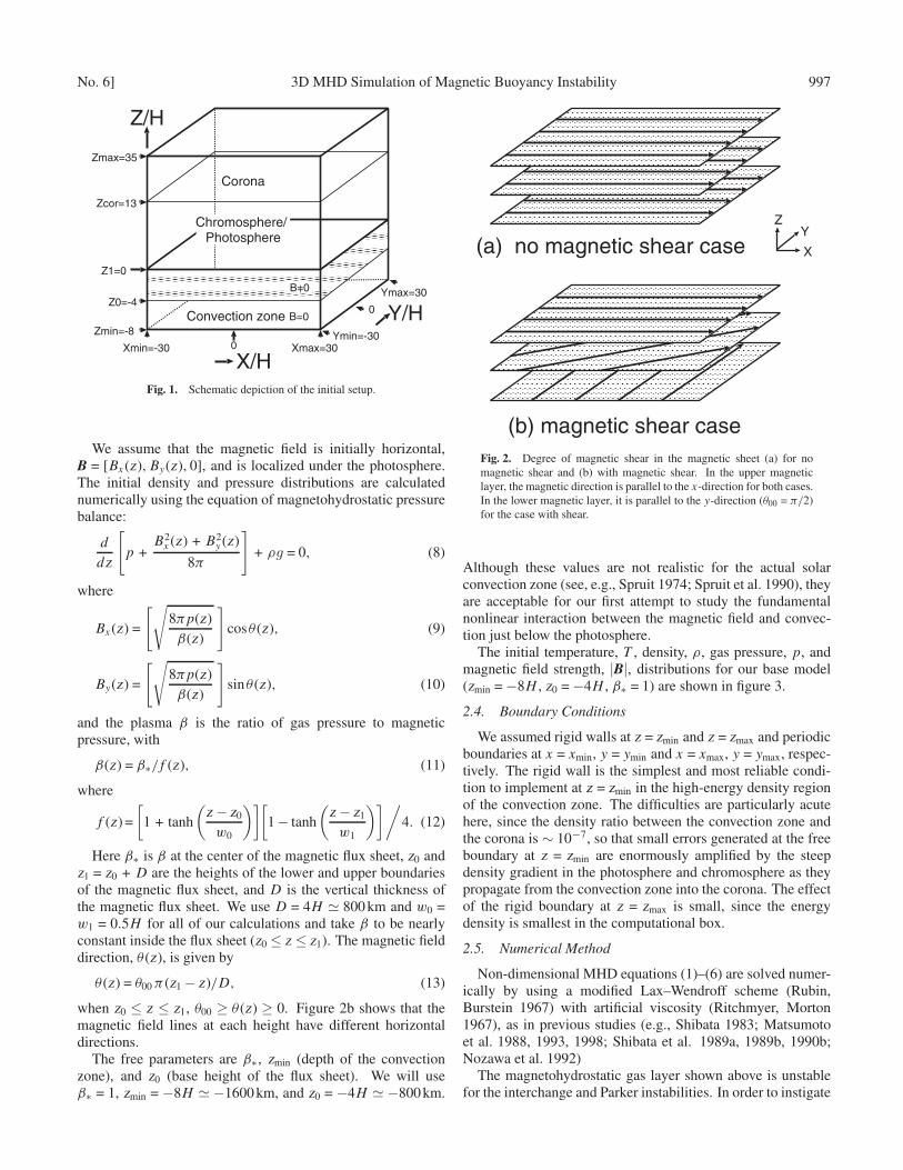
when z0 ≤ z ≤ z1, θ00 ≥ θ (z) ≥ 0. Figure 2b shows that themagnetic field lines at each height have different horizontaldirections.

The free parameters are β∗, zmin (depth of the convectionzone), and z0 (base height of the flux sheet). We will useβ∗ = 1, zmin = −8H � −1600 km, and z0 = −4H � −800 km.

Fig. 2. Degree of magnetic shear in the magnetic sheet (a) for nomagnetic shear and (b) with magnetic shear. In the upper magneticlayer, the magnetic direction is parallel to the x-direction for both cases.In the lower magnetic layer, it is parallel to the y-direction (θ00 = π/2)for the case with shear.

Although these values are not realistic for the actual solarconvection zone (see, e.g., Spruit 1974; Spruit et al. 1990), theyare acceptable for our first attempt to study the fundamentalnonlinear interaction between the magnetic field and convec-tion just below the photosphere.

The initial temperature, T , density, ρ, gas pressure, p, andmagnetic field strength, |B|, distributions for our base model(zmin = −8H , z0 = −4H , β∗ = 1) are shown in figure 3.

2.4. Boundary Conditions

We assumed rigid walls at z = zmin and z = zmax and periodicboundaries at x = xmin, y = ymin and x = xmax, y = ymax, respec-tively. The rigid wall is the simplest and most reliable condi-tion to implement at z = zmin in the high-energy density regionof the convection zone. The difficulties are particularly acutehere, since the density ratio between the convection zone andthe corona is ∼ 10−7, so that small errors generated at the freeboundary at z = zmin are enormously amplified by the steepdensity gradient in the photosphere and chromosphere as theypropagate from the convection zone into the corona. The effectof the rigid boundary at z = zmax is small, since the energydensity is smallest in the computational box.

2.5. Numerical Method

Non-dimensional MHD equations (1)–(6) are solved numer-ically by using a modified Lax–Wendroff scheme (Rubin,Burstein 1967) with artificial viscosity (Ritchmyer, Morton1967), as in previous studies (e.g., Shibata 1983; Matsumotoet al. 1988, 1993, 1998; Shibata et al. 1989a, 1989b, 1990b;Nozawa et al. 1992)

The magnetohydrostatic gas layer shown above is unstablefor the interchange and Parker instabilities. In order to instigate


Fig. 3. One-dimensional (z-) distribution of the initial density (solidcurve), pressure (dashed curve), magnetic field strength (dash-dottedcurve), and temperature (dotted curve). ρ0, p0, T0, and B0 denotethe initial density, pressure, temperature, and magnetic field strengthat z = zmin (z = −8H ), respectively.

instability, small velocity perturbations of the form

Vz = f (z)ACs cos(

2πx

λx

)cos

(2πy

λy

)(14)

are given initially within the finite horizontal domain (|x,y| ≤λ/2), where λ is the wavelength of the small velocity pertur-bations. A typical case is λx = λy (ky/kx = 1). Here Cs isthe sound velocity in the photosphere and A (= 10−3) is themaximum value of Vz/Cs in the initial perturbation. In the 2Dcase (model 1), a small velocity perturbation is used, of theform

Vx = f (z)ACs sin(

2πx

λ

)(15)

Although the distribution of the velocity given by equation(14) is not exactly an eigenfunction, the growth rate of theperturbation in the linear regime agrees well with that obtainedfrom an exact linear analysis, as will be discussed in theAppendix (see also Matsumoto et al. 1988; Shibata et al.1989a).

The mesh size is ∆z0 = 0.15H for z ≤ zcor, which slowlyincreases up to ∆zmax = 0.375H = Tcor/(10×∆z0) for z ≥ zcor.

Table 1. Models and parameters.

Model 2D or 3D kxH or kH λ/H Shear ky : kx

1 2D 0.31 20 0.0 · · ·2 3D 0.5 12.6 0.0 1 : 13 3D 0.5 12.6 0.5π 1 : 14 3D random random 0.0 1 : 15 3D random random 0.5π 1 : 16 3D 0.5 12.6 0.0 2 : 17 3D 0.5 12.6 1.0π 2 : 18 3D 0.5 12.6 2.0π 2 : 1

Fig. 4. 2D distributions of (a) magnetic field strength |B| =√B2

x + B2z (colors), velocity field (vectors) and density (contour lines)

and (b) magnetic field lines (lines) and density (gray scale colors) att/τ0 = 80 for the 2D case (model 1). The velocity length 1H is 1 Cs(sound velocity).

The other parameters are ∆x, ∆y = 0.2. The total numberof mesh points is Nx × Ny × Nz = 300 × 300 × 203 and thetotal area is [(xmax − xmin) × (ymax − ymin) × (zmax − zmin)] =(60H ×60H×43H ). The parameters of the models consideredhere are summarized in table 1.

3. Nonlinear Simulation Results

3.1. 2D Case (Model 1)

Let us first discuss the typical nonlinear evolution of theParker instability in the 2D case. Figures 4 and 5 show typicalresults for the no-shear mode.

All results agree with those of Shibata et al. (1989a), exceptfor the time sequence; the time evolution of the emerging fluxloop is slow, compared with that of Shibata et al. (1989a,1989b), because the perturbation amplitude, A, is taken to be10−3. A self-similar evolution for the density (figure 5b) andmagnetic field strength can be seen in figure 5d,


Fig. 5. z-distribution: (a) the vertical component velocity (Vz ), (b) thedensity (log ρ), (c) the local Alfven velocity (VA), (d) the horizontalcomponent of the magnetic field (log B), (e) the magnetic pressure[log(∆Pm/∆z)], and (f) plasma β (gas pressure/magnetic pressure) atx = 0H (middle of the rising loop) for model 1 (the case shown infigure 4) at t/τ0 = 0 (the thinnest line), 50, 60, 70, and 80 (the thickestline).

ρ ∝ z−4 and B ∝ z−1. (16)

In particular, the plasma β decreases to less than 0.1,which indicates that the magnetic pressure dominates overthe gas pressure and the magnetic loop continues to increase(figure 5f). The dominance of the magnetic pressure leads tothe formation of a current-free magnetic loop.

3.2. No Magnetic Shear with a Localized Perturbation(Model 2)

Let us now discuss the 3D cases. Figures 6, 7, and 8 showtypical results for the no-shear mode. Figure 6c indicatesthat the magnetic field in the y-direction emerges from thenarrow region and expands horizontally in the photosphere.The 3D displays in figure 7 show that the magnetic field linesbecome almost vertical in the region where the magnetic fieldis concentrated.

In the upper photosphere, the magnetic field is parallel to thephotospheric plane and expands horizontally. Since the scaleheight of the photosphere is smaller than the thickness of a

Fig. 6. Nonlinear simulation results for no magnetic shear, where aninitial localized perturbation is assumed (model 2). (a) Distribution ofVz on the photosphere surface (z = 0H ). (b) Velocity distribution inthe upper photosphere (z = 7H ). Magnetic field (colors), velocity field(vectors), and density (contour lines) on the (c) y–z surface and (d) x–zsurface.

magnetic sheet, the gas pressure outside the sheet decreasesrapidly. Hence, when the magnetic field slightly emergesinto the photosphere, the magnetic flux expands horizontallyuntil the magnetic pressure of the sheet is balanced with thesurrounding gas pressure.

The velocity vectors also show that plasma expands inthe horizontal direction more than in the vertical direction(see figures 6b, c, d). This result implies that the rise of themagnetic loop stops at lower heights (< 10H ) and the distri-bution of the magnetic pressure is in a new state of magneto-hydrostatic equilibrium. The characteristic wavelength of themagnetic loop is dependent on the width 2–6H (see line C–Din figures 6a, c) in the photosphere (z = 0) in the y-direction.Another characteristic wavelength is the comparatively long27–32H (line A–B in figures 6a, d), which indicates expan-sion of the magnetic loop in the x-direction in the photo-sphere (z = 0). However, at z = 7H (the lines E–F and G–Hin figure 6b), the characteristic wavelengths in both the x-and y-directions increase to 35–40H , because of the inversecascade effect (Hachisu et al. 1992).

In figure 8a at t/τ0 = 50, 60, and 70, the top of the magneticloop reaches z ∼14H . In the last stage, the magnetic loop doesnot rise further. Figures 8b, d, e show the distributions of thedensity, magnetic field strength, and magnetic pressure, whichare approximated by

B ∝ exp(−∆z

HB

), ρ ∝ exp

(−∆z

Hρ

),

Pm ∝ exp(− ∆z

HPm

)∝ exp

(−2∆z

HB

),

(17)

with HB ∼ 4.8, Hρ ∼ 2.4, and HPm ∼ 2.4. What are the


Fig. 7. Perspective view of the magnetic field at the epoch t/τ0 = 55 for no magnetic shear, where an initial sinusoidal perturbation is assumed (model 2).The five red tubes show the magnetic field lines that are connected to the points (x,y,z) = [(−10.6H,−5.3H,0H,5.3H,10.6H ),0H,5H ] and the fiveblue tubes show the magnetic field lines that are connected to (x,y,z) = [(−8.4H,−4.2H,0H,4.2H,8.4H ),0H,14H ].

Fig. 10. Perspective view of the magnetic field at the epoch t/τ0 = 55 for the case with magnetic shear, where an initial sinusoidal perturbation isassumed (model 3).

physical meanings of these distributions? They are similarto typical distributions of the magnetic field and plasma inmagnetohydrostatic equilibrium with uniform temperature andconstant plasma β when the magnetic field is horizontal. Infact, an exact equilibrium solution predicts Hρ = (1 + 1/β) andHPm = Hρ . In our simulation results, β ∼ 0.7 (see figure 8f), sowe have Hρ ∼ 2.4, which is consistent with direct simulation

results. The relations Hρ = HPm = HB/2 are also consistent withmagnetohydrostatic equilibrium theory.

Note that the plasma β ∼ 0.7 in the rising magnetic loopis larger than that in the 2D case (β ∼ 0.1). This is becausethe magnetic flux rapidly expands in the horizontal directionin the photosphere, so that the magnetic field becomes weak.Hence, the magnetic flux cannot expand into the corona and


Fig. 8. z-distribution at (x,y) = (0H,0H ) (middle of the rising loop) for model 2 (no-shear mode) shown in figure 6 at t/τ0 = 0, 50, 60, and 70, withall other details of the graphs being the same as in figure 5. The dashed lines in (b), (d), and (e) indicate the lines of ρ ∝ exp (−∆z/Hρ ) with Hρ = 2.4,B ∝ exp (−∆z/HB ) with HB = 4.8, and Pm ∝ exp(−∆z/HPm ) with HPm = 2.4, respectively. In (f) the dashed line is β = 0.7.

instead tends to be in magnetohydrostatic equilibrium in thephotosphere and chromosphere.

3.3. Magnetic Shear with a Localized Perturbation (Model 3)

Figures 9, 10, and 11 show the results of 3D calculationsfor the shear mode. In figures 9a and 10, the loop that passesthrough the origin (x =0, y =0) emerges at an angle∼45◦ to thex-direction, while for the case of no-shear the loop is parallel tothe x-direction. This is because the magnetic sheet at the depthwhere the field line is at 45◦ rises up into the photosphere att/τ0 = 50. In the last stage of the calculation after t/τ0 = 50, adeeper magnetic sheet rises and becomes a loop with an anglegreater than 45◦.

Figure 9c indicates that the area where the magnetic sheet

rises in the photosphere is larger than that for the no-shearcase. In the shear case, the velocity vectors show that theplasma expands in the horizontal direction more than in thevertical direction (see figures 9b, c, d) and the magnetic fieldexpands at medium heights (6–12H ). Figure 9a shows that thecharacteristic wavelength in the x-direction is comparativelylong 13H (the line A–B) and the characteristic wavelength inthe 45◦-direction is somewhat short 4–8H (the line C–D).

The same as in the no-shear case, the plasma density andmagnetic field strength distributions in the shear mode can alsobe approximated by exponential functions [equation (17)] withHρ ∼ 2.1, HB ∼ 4.2 (see figures 11b, d) and the plasma β ∼ 0.9in the magnetic loop (see figure 11f).


Fig. 9. Nonlinear simulation results for magnetic shear, where aninitial sinusoidal perturbation is assumed (model 3). The details of thegraphs are the same as in figure 6.

3.4. Random Perturbation (Model 4 and Model 5)

Figure 12 shows the results for a random initial perturba-tion for both the no-shear and shear modes. In the earlystage [� t/τ0 = 30 (see figures 12a,d)] the characteristic wave-length in the y-direction is small and equal to λ = 3.5H

(∼ 60H/17). Subsequently the wavelength increases to λ =4.6H (∼ 60H/13) at t/τ0 =40 (see figures 12b, e) and λ=5.5H

(∼ 60H/11) at t/τ0 = 50 (see figures 12c, f). In figure 13b, d,at t/τ0 = 50 the magnetic loop rises at z = 19H in the no-shearcase and at z = 13H in the shear case. The distributions ofplasma density and magnetic field are basically the same asthose in previous 3D cases [equation (17)].

3.5. Loop Height for Different Shear Cases

Figures 14 and 15a, b, c, d show the loop height for eachsimulation result at t/τ0 = 55 and the maximum loop height.When ky/kx < 1, the Parker instability is easily caused, soeach loop height rises comparatively high, to 15–24H at t/τ0 =55 and over 30H at maximum height. On the other hand,for ky/kx > 1, the interchange instability occurs easily andthe height monotonically decreases when ky is large. Whenky/kx < 1, h/Lx and h/Ly are almost 0.3–0.5, and thereforethe loop expands horizontally. This is due to the stabilizingeffect of magnetic shear in the interchange mode.

Figure 15e shows the plasma β for each simulation result.When the shear angle, θ00, is large and ky/kx is small, the β

value monotonically decreases (the low β regime). In partic-ular, when θ00 > 2π , the averaged plasma β is almost constantagainst ky/kx . Figures 16a, b, c show that the loop heightincreases and the plasma β decreases for shear angles of θ00 =0,π , and 2π when ky/kx = 2. When θ00 becomes large, the formof the emerging magnetic loop changes to a dome-like struc-ture, because the horizontal expansion of the loop is inhibited

Fig. 11. z-distribution at (x,y) = (0H,0H ) (middle of the rising loop)for model 3 (shear mode) shown in figure 9 at t/τ0 = 0, 50, 60, and 70.The details of the graphs are the same as in figure 8. The dashed lines in(b), (d), and (e) indicate the lines of ρ ∝ exp(−∆z/Hρ ) with Hρ = 2.1,B ∝ exp (−∆z/HB ) with HB = 4.2, and Pm ∝ exp (−∆z/HPm ) withHPm = 2.1, respectively. In (f) the dashed line is β = 0.9.

by the magnetic shear.

4. Summary and Discussion

4.1. Summary

The 3D simulations show the following:

• When the magnetic field emerges into the photospherewith a localized and random initial perturbation, the fluxexpands horizontally and does not go upward. At thattime, the distributions of magnetic field strength, density,and pressure can be written as exp (−∆z/H(B,ρ,Pm)), asin magnetohydrostatic equilibrium, and the plasma β ofthe magnetic loop is 0.3–1.3 (the magnetic field strengthis weak).

• The plasma β of the magnetic loop is larger (∼0.01–0.1)than that of the 2D case. When an initial periodic pertur-bation is assumed, the emerging flux rises to the coronaand the magnetic field expands like a potential field as inthe typical 2D case.


Fig. 12. Nonlinear simulation results for the no-magnetic shear mode(left; a, b, c: model 4) and for the magnetic shear mode (right; d, e,f: model 5), where a random-noise perturbation is initially assumed.These figures show a distribution of Vz on the photosphere surface(z = 0H ) at t/τ0 = 30, 40, and 50.

• When there is no magnetic shear, the magnetic fluxcannot rise as a whole (i.e., as a global or thick magneticloop), but rises as fragmented flux tubes because of theinterchange instability. In this case, the flux tubes expandsignificantly in the horizontal direction, so that theaverage magnetic pressure decreases greatly and hencethe tube soon stops at a low height. However, when thereis magnetic shear, the interchange mode is stabilized (seethe Appendix for a linear stability analysis), so that thetube can rise as a whole and hence the height of the loopincreases (see figure 15). For the same reason, the loopheight increases with the shear angle or ky .

4.2. Discussion

Shibata et al. (1989a) and other studies have shown thatin 2D calculations the emerging magnetic flux rises into thecorona with a density given by ρ ∝ z−4 and a magnetic fieldgiven by Bx ∝ z−1, due to a potential magnetic field. In themomentum equation, the gravity term, ρ g ∼ z−4, is smallerthan the magnetic term, B2/dz ∼ z−3, and therefore the expan-sion of the magnetic loops does not stop in the 2D model.

Fig. 13. Nonlinear simulation results at t/τ0 = 50 for the no-shearmode (left) and for the magnetic shear mode (right), where a randomnoise perturbation is initially assumed (model 4 and model 5). Theupper figures show the distribution of Vz on the upper photospheresurface (z = 7H ) and the lower figures show the magnetic field (colors),velocity field (vectors) and density (contour lines) on the x–y surface.

When an initial periodic perturbation is assumed, theemerging flux rises into the corona and the magnetic fieldexpands like a potential field. This special case is similar tomodel 10 of Matsumoto et al. (1993), where initially straightmagnetic tubes are placed side by side. Because the emergenceof each tube occurs at the same time, the expansions areblocked in the horizontal direction by each other and hencethey rise in the vertical direction. In this case the emergingloop structure is similar to the 2D case (see figure 17a).

This result explains why a twisted magnetic tube rises intothe corona in the studies of Magara and Longcope (2003) andFan and Gibson (2004). The tube is twisted very strongly.Because the interchange instability occurs on the surface ofthe tube, the flux tube expands both horizontally and verti-cally. The horizontal expansion is blocked on both sides byother emerging fluxes. However, after the photosphere is fullof magnetic field, the flux emerges from the upper photosphereto the corona in a realistic simulation of the solar atmosphere(see figure 13b). The critical wavelength λc in the photosphereis estimated to be

λc ∼ 2πH

(1 +

1β

). (18)

When β = 0.5, we find λc ∼ 18H . In fact, figure 13b showsthat the wavelength of the emerging flux into the corona isroughly ∼ 18H , in agreement with the above estimate. Asan initial localized perturbation is assumed, the emerging fluxexpands in the photosphere (see figure 17b). When an initialrandom perturbation is also assumed, the top of each loop ofthe emerging flux is different and the magnetic loop expandshorizontally, like the growth of the localized perturbation loop(see figure 17c).


Fig. 14. Definitions of h, Lx , and Ly in a loop.

In figure 18 at t = 15–20 min, the expansion velocity in thehorizontal direction is 10–15 km s−1 and the magnetic fieldstrength is ∼ 10 gauss. This velocity is estimated by assumingthat the kinetic energy is equal to the magnetic energy,ρv2 ∼ B2/(8π ). Where ρ ∼ p/C2

s and v2 ∼ B2/(8πp/C2s ) =

C2s /β. If β = 1, v ∼ 1Cs = 10 km s−1. Although this

velocity is large compared to the observed typical value for thephotosphere, the expansion time-scale is very short (� 5 min,see figure 18b) and the size is small (� 4000 km). Thereforesuch phenomena may be observed by the high resolution LaPalma, Swedish Vacuum Solar Telescope (De Pontieu et al.2004). Future observations, using Solar-B for example, willreveal the detailed features of the emerging flux.

The author would like to thank Prof. K. Shibata and allthe members of Kwasan Observatory, Kyoto University forfruitful discussions and help. The author is also grateful toDr. D. Brooks for his careful reading of the manuscript andmany valuable comments. This work was carried out by thejoint research program of the Solar-Terrestrial EnvironmentLaboratory, Nagoya University. This work was supportedin part by the JSPS Japan-UK Cooperation Science Program(principal investigators: K. Shibata and N. O. Weiss).

Appendix. Linear Stability Theory and Comparison withNonlinear Simulation

A.1. Linear Theory

In order to study the main characteristics of the linear insta-bility of the magnetic flux sheet with magnetic shear, weanalyze the linear stability of the flux sheet with a normal-mode method similar to that of Horiuchi et al. (1988). Weconsider the growth of a small perturbation that has a functionalform δW ∝ exp(iωt + ikxx + ikyy), where W is the physicalquantity (ρ, p, v, B), and δW is its perturbation. The linearizedequations are the same as those in Horiuchi et al. (1988) andNozawa et al. (1992) and the eigenvalue (ω) and eigenfunctionare calculated numerically.

Figure 19 shows the growth rates iω as a function ofhorizontal wave number kH = H

√(k2

x + k2y) for two cases,

(a) the no-shear mode and (b) the shear mode, when β∗ = 1,γ = 1.05, D = 4H , zmin = −8H , z0 = −4H , zcor = 13H ,and Tcor/Tph = 25. The numbers attached to each curveindicate the ratio ky/kx . When the wavenumber along thefield line (kx) is fixed, the growth rate increases with the

Fig. 15. Normalized loop height (a, b, c: h/H , h/Lx , h/Ly ) as afunction of ky/kx at t/τ0 = 55 for a localized perturbation. The numbersindicate the shear angle, θ00 (radian). Here, h is the height of theemerging flux loop, Lx the half length of the loop, and Ly the width ofthe loop (see figure 14). Also shown are (d) the maximum heights ofthe loop and (e) the values of the averaged plasma β (see figure 11f).

perpendicular wavenumber, ky . Thus, a perturbation with ashorter wavelength perpendicular to the magnetic field linegrows faster than perturbations with longer wavelengths.

The linear growth rate of the non-sinusoidal perturba-tions (14) is the same as that of the sinusoidal perturba-tions (single plane wave) in the shear mode because the non-sinusoidal perturbation can be decomposed into two planewave perturbations whose wave vectors are (kx, ky) and(kx,−ky).

Since the perturbations are added in the direction parallelto the magnetic field on the top surface of the flux sheet, theParker mode dominates at long wavelengths (ky/kx = 0), wherethe linear analytic growth rate has a relative maximum valueiw ∼ 0.124 at kH = 0.275 (λ = 23H ).

When ky/kx = 0, the growth rate is larger for the no-shearmode (a) than that for the shear mode (b). This is because theinterchange mode is coupled in (b), even for ky = 0, since thereis a layer where kx ⊥ B in the sheared flux sheet.

On the other hand, the growth rate is generally smaller in (b)


Fig. 16. Nonlinear simulation results for shear angles of θ00 = 0 (left; a, d) at t/τ0 = 50, π (middle; b, e) at t/τ0 = 55, and 2π (right; c, f) at t/τ0 = 55when ky/kx = 2 (models 6, 7 and 8) for (a, b, c) the x–y surface (see figure 6d) and (d, e, f) the plasma β distribution in z at (x, y) = (0H,0H ) (seefigure 8f).

Fig. 17. Schematic pictures of emergence in (a) strong twisted flux tube, (b) weak twisted flux tube or magnetic flux sheet, and (c) random perturbationwith no magnetic shear.

Fig. 18. Time evolution of the y-component of the velocity andmagnetic strength at x = 0H , y = 10H , z = 5H for model 2.

Fig. 19. Normalized growth rate (in units of Cs/H ) as a function of k

(kH =√

k2x + k2

y H ) for ky/kx = 0, 1, 2, 4, and ∞ (1.0e10) for (a) theno-shear mode and (b) the magnetic shear mode. β∗ = 1.0 and γ = 1.05are assumed.


Fig. 20. Time evolutions of the x-component of the velocity at z = 0 for models 1, 4, and 5. (a) Mode analysis and time evolution of log |Vx |. The fullline is λ = 60H (k′ = 1, kH = 0.10), the dashed line k′ = 2 (λ = 30H , kH = 0.21), the dot-dashed line k′ = 3 (λ = 20H , kH = 0.31), the dotted line k′ = 4(λ = 15H , kH = 0.42), and the full line with ∗ the time evolution of log |Vx/Cs| at the point (x,y,z) = (0,0,0). The dotted line represents the growth rateobtained from linear stability analysis (iω = 0.124) for λ = 20H (k′ = 3, kH = 0.314). Also shown are (b) the no-shear mode and (c) the shear mode oflog |Vz |, with the meanings of the lines being the same as in (a).

than in (a) for short wavelengths. This is because the inter-change mode tends to be stabilized by the magnetic tensionforce in the sheared magnetic field.

Therefore, for the shear mode (b), the maximum growth rateof ky/kx = 0 is larger than that of ky/kx = 1,2, as the bottom ofthe sheet is unstable because kx ⊥ B.

With B = 0 and ky/kx = 1010 for the no-shear mode, thegrowth rate does not have a maximum and increases monoton-ically with the wavenumber. The growth rate in this case is thesame as the pure Rayleigh–Taylor instability, which is am

√kg.

Here, am is a parameter of the magnetic interchange instability,and has a value of 0.33.

A.2. 2D and 3D Nonlinear Simulations with Single orRandom Perturbations

The horizontal wavelength (λ/H = 20) of the initial pertur-bation is close to the wavelength of the maximum growth rate

for β = 1; the growth rate is 0.12 (see the thick dotted line infigure 20a). Since the perturbation given in the initial conditionis not an eigenfunction, the most unstable wavelength does notgrow, but other modes are excited by the nonlinear effect. Theabove results show that the instability grows on the wavelengthgiven in the initial conditions in the 2D case.

Figures 20b, c show the results for a random initial perturba-tion for both the no-shear and shear modes. It is found that thegrowth rate in this case is 0.4. Comparing this value with lineartheory, we find the corresponding wavenumber is kH = 1.7(λ = 3.7H ) for ky/kx = ∞. This λ = 3.7H is consistent with18 × ∆x (= ∆y = 0.2H ), which agrees with the maximumwavelength resolution of the numerical scheme.

References

Baierlein, R. 1983, MNRAS, 205, 669Basu, S., Mouschovias, T. Ch., & Paleologou, E. V. 1997, ApJ, 480,

L55Cattaneo, F., Chiueh, T., & Hughes, D. W. 1990, Journal of Fluid

Mechanics, 219, 1Chou, W., Tajima, T., Matsumoto, R., & Shibata, K. 1999, PASJ, 51,

103De Pontieu, B., Erdelyi, R., & James, S. P. 2004, Nature, 430, 536Fan, Y. 2001, ApJ, 554, L111Fan, Y., & Gibson, S. E. 2004, ApJ, 609, 1123Hachisu, I., Matsuda, T., Nomoto, K., & Shigeyama, T. 1992, ApJ,

390, 230Hanawa, T., Matsumoto, R., & Shibata, K. 1992, ApJ, 393, L71Hanasz, M., Otmianowska-Mazur, K., & Lesch, H. 2002, A&A, 386,

347

Horiuchi, T., Matsumoto, R., Hanawa,T., & Shibata, K. 1988, PASJ,40, 147

Hughes, D. W., & Proctor, M. R. E. 1988, Annual Review of FluidMechanics, 20, 187

Ishii, T. T., Kurokawa, H., & Takeuchi, T. T. 1998, ApJ, 499, 898Kamaya, H., Mineshige, S., Shibata, K., & Matsumoto, R. 1996, ApJ,

458, L25Kim, J., Franco, J., Hong, S. S., Santillan, A., & Martos, M. A. 2000,

ApJ, 531, 873Kim, J., Hong, S. S., Ryu, D., & Jones, T. W. 1998, ApJ, 506, L139Kim, J., Ryu, D., & Jones, T. W. 2001, ApJ, 557, 464Kim, W., Ostriker, E. C., & Stone, J. M. 2002, ApJ, 581, 1080Kruskal, M. D., & Schwarzchild, M. 1954, Proc. R. Soc. London,

Ser. A, 223, 348Kurokawa, H. 1989, Space Science Reviews, 51, 49


Kurokawa, H., Wang, T., & Ishii, T. T. 2002, ApJ, 572, 598Kusano, K., Moriyama, K., & Miyoshi, T. 1998, Physics of Plasmas,

5, 2582Magara, T. 2004, ApJ, 605, 480Magara, T., & Longcope, D. W. 2001, ApJ, 559, L55Magara, T., & Longcope, D. W. 2003, ApJ, 586, 630Matsumoto, R., Horiuchi, T., Shibata, K., & Hanawa, T. 1988, PASJ,

40, 171Matsumoto, R., & Shibata, K. 1992, PASJ, 44, 167Matsumoto, R., Tajima, T., Chou, W., Okubo, A., & Shibata, K. 1998,

ApJ, 493, L43Matsumoto, R., Tajima, T., Shibata, K., & Kaisig, M. 1993, ApJ, 414,

357Matthews, P. C., Hughes, D. W., & Proctor, M. R. E. 1995, ApJ, 448,

938Nozawa, S., Shibata, K., Matsumoto, R., Sterling, A. C., Tajima, T.,

Uchida, Y., Ferrari, A., & Rosner, R. 1992, ApJS, 78, 267Parker, E. N. 1955, ApJ, 121, 491Parker, E. N. 1966, ApJ, 145, 811Parker, E. N. 1979, Cosmical Magnetic Fields (Oxford: Clarendon

Press)

Ritchmyer, R. D., & Morton, K. W. 1967, Difference Methods forInitial-Value Problems, 2nd ed. (New York: Interscience)

Rubin, E. L., & Burstein, S. Z. 1967, J. Comp. Phys., 2, 178Ryu, D., Kim, J., Hong, S. S., & Jones, T. W. 2003, ApJ, 589, 338Shibata, K. 1983, PASJ, 35, 263Shibata, K., & Matsumoto, R. 1991, Nature, 353, 633Shibata, K., Nozawa, S., Matsumoto, R., Sterling, A. C., & Tajima, T.

1990a, ApJ, 351, L25Shibata, K., Tajima, T., & Matsumoto, R. 1990b, ApJ, 350, 295Shibata, K., Tajima, T., Matsumoto, R., Horiuchi, T., Hanawa, T.,

Rosner, R., & Uchida, Y. 1989a, ApJ, 338, 471Shibata, K., Tajima, T., Steinolfson, R. S., & Matsumoto, R. 1989b,

ApJ, 345, 584Spruit, H. C. 1974, Sol. Phys., 34, 277Spruit, H. C., Nordlund, A., & Title, A. M. 1990, ARA&A, 28, 263Tajima, T., & Shibata, K. 1997, Plasma Astrophysics (Reading,

Massachusetts: Addison-Wesley)Zwaan, C. 1985, Sol. Phys., 100, 397Zwaan, C. 1987, ARA&A, 25, 83

three-dimensional magnetohydrodynamic simulation of nonlinear magnetic...

Documents