Three-dimensional Fluorescence Lifetime Imaging in

Confocal Microscopy of Living Cells

Larisa Baiazitova, Vratislav Čmiel, Josef Skopalík, Ondřej Svoboda, Ivo Provazník

Department of Biomedical Engineering

Brno University of Technology

Brno, Czech Republic

provaznik@feec.vutbr.cz

Abstract—Fluorescence lifetime imaging (FLIM) is a modern

optical method which increases the potential of standard

microscopy. This paper shows the possibilities of extended

fluorescence lifetime evaluation and imaging in studying three-

dimensional structures such as compartments of living cells with

different fluorescence lifetimes. The method for quasi-FLIM

image calculation is presented and image processing steps useful

for biological experiments are suggested. The method was tested

on isolated cardiomyocyte cells (CMs) and rat bone marrow

stromal cells (MSCs) labelled with SPIO-rhodamine

nanoparticles and stained with standard fluorescent dyes. We

proved it is possible to use an exponential decrease of

fluorescence in time and lifetime parameters for pseudo-colour

3D image mapping of living cells and their compartments that is

not a standard function of confocal microscopes.

Keywords—fluorescence lifetime; FLIM; cardiomyocyte;

stromal cell; image segmentation

I. INTRODUCTION

Fluorophore fluorescence is characterised by the absorption spectrum, quantum yield, emission spectrum, and the fluorescence lifetime. Fluorophore excitation and the emission spectrum are used to sense the local environment of a fluorophore (e.g. local ion concentration, electric potential [1]). The fluorescence lifetime difference of some specific organic compounds makes it possible to monitor fast processes in biological experiments (typically on nanosecond and microsecond levels). The fluorescence lifetime difference in 3D images has been used by our team in several special applications such as the long-time monitoring of cardiomyocytes viability [2], [3] or the evaluation of cheese pH at the microscale level [4]. Besides the pH value or vitality markers in cells, temperature in different parts of the cell [5], acidity or salinity [6], hydrostatic pressure, and oxygen concentration [7] are also possible to monitor on the basis of fluorescence lifetime detection.

Today, fluorophores are used in biological and medical applications mainly for two basic purposes: (i) determination of protein/DNA incidence (fluorophore with affinity to certain proteins and DNA structures in living cells [8], [9]) and (ii) for measuring ion or gas concentrations in fluorophore environments (in tissue or subcellular compartments [10], [11]). In comparison to the quantum yield and spectral shift of fluorescence, fluorescence lifetime is not a common marker. The main reason for this could be found in the excessive cost

of photodetectors for precise time resolution for lifetime quantification. Their availability was limited only to the most excellent labs in last decades. However, today the cost of detectors is decreasing and the fluorescence lifetime will be measurable also by lower-cost microscopy setup in the next few years.

FLIM is a modern method of visualisation which increases the potential of standard microscopy. In biological samples, FLIM has three basic applications: (i) to distinguish between two fluorescence markers which have the same excitation spectra but different lifetime, (ii) to quantify some physical or chemical value in subcellular regions, and (iii) to map local protein interactions using FRET (Fluorescence Resonance Energy Transfer).

Image segmentation plays a crucial role in biological and medical imaging applications by enhancing the detection of biological structures of interest. Existing medical image segmentation methods are typically based on spectral clustering, normalised cuts [12], [13], [14] and the mixture of Gaussian distributions [15]. The portfolio of FLIM image software compatible with data from Leica or another confocal microscope is very limited to date and there is no published method for automatic segmentation of FLIM images.

Our goal is to show the extended possibilities of fluorescence lifetime evaluation of three-dimensional structures, especially in the case of segmentation of intracellular compartments with different fluorescence lifetimes. The presented custom-made software utility represents an economical and user-friendly tool for big data processing applicable to the elaboration and analysis of confocal scan visualisation of tissue in the fluorescence lifetime mode. The tool also allows the final transformation of data to high-quality pseudo-colour 3D images. This use was tested on data from isolated CMs and rat bone MSCs labelled with superparamagnetic fluorescence iron oxide (SPIO) nanoparticles (red fluorescence), DAPI (blue fluorescence), and calcein AM (green fluorescence) fluorescent probes. Different parts of the cells display different fluorescence lifetimes and thus the lifetime is specific for certain organelles. This difference can be used for the precise delineation of organelles in 3D space mostly without the need of expensive or complicated staining or antibodies.

2017 25th European Signal Processing Conference (EUSIPCO)

ISBN 978-0-9928626-7-1 © EURASIP 2017 469

II. MATERIALS AND METHODS

A. Fluorescence Lifetime Detection

Experiments were performed using the confocal laser scanning microscope Leica TCS SP8 X equipped with gateable hybrid (HyD) detectors as internal spectral detectors. The picosecond White Light Laser (WLL) Leica Microsystems is freely tuneable in the spectral range 470–670 nm with an 80 MHz repetition rate used for excitation. The combination of gateable HyD detectors and WLL enabled custom defined experiments. The time-resolved settings of the HyD detectors were adapted by the TimeGate function that allows the arbitrary setting of a time band in the range of 0–12 ns with the minimum opening time 3.5 ns. That function increases the confocal image quality and contrast by inserting a time pause (usually a fraction of a nanosecond) between excitation and detection.

The sequence of images is acquired with different acquisition-detection spacing that is defined with step k and with specific TimeGate window width as w (see Fig. 1.).

Fig. 1. Acquisition-detection spacing in quasi-FLIM. Intensity of fluorescence after laser pulse (red curve) and illustration of time windows for

detection of integrated signal (grey boxes).

A real fluorescence intensity signal from each sample pixel (which is equivalent to about 0.01 µm2 of the sample) decreases in time as I(t):

𝐼(𝑡) = 𝐼0𝑒𝛽𝑡 (1)

The microscope’s detection system is not able to measure the exact fluorescence curve (with ideal sub-nanosecond time resolution), however, the system can integrate the fluorescence

signal in the detection window a, b (usual setting of w = 3 ns) and repeat this detection in several next detection windows

a+n*k, b+n*k>; n ∈ N; k is step 0.1 ns or more, which is

illustrated by the grey boxes in Fig. 1. The integral intensity for each pixel of the sample and each time detection window is:

∫ 𝐼(𝑡)𝑑𝑡𝑏+𝑘

𝑎+𝑘 a, b, k ∈ R+ (2)

and this value is derived by the confocal microscope and saved

in a data matrix (one matrix for one time interval a+n*k, b+n*k>, one matrix contains one value for each pixel of the

sample). These data matrices are input for our software.

Tangent s of the logarithmed I(t) can be expressed as:

𝑠 = 𝑙𝑛 [∫ 𝐼(𝑡)𝑑𝑡𝑏+𝑘

𝑎+𝑘] − 𝑙𝑛 [∫ 𝐼(𝑡)𝑑𝑡

𝑏

𝑎] a, b, k ∈ R+

(3)

With derivation, s is simplified to

𝑠 = 𝛽𝑘 (4)

and fluorescence lifetime can be calculated more easily. This method is based on quasi-FLIM computing, where the intensity image sequence together with parameters k and w are used (the lines are obtained and their tangents calculated by I(t) logarithmization). The method and its output are described in Fig. 2.

B. Quasi-FLIM Data Processing Method

Prior to data processing, the software loads an image sequence (a typical sequence is illustrated in Fig. 4.) with known parameters of a TimeGate window w and step size k (see Fig. 1.). The following step is to suppress specific background noise in the original image, thus we may apply a simple but efficient median filter. Then, a decrease of the fluorescence intensity signal is determined in each pixel. Thus, we can get a curve and then calculate a fluorescence lifetime from the data. The original images are pseudo-coloured according to the selected scale.

Fig. 2. Generating quasi-FLIM image by the presented method.

3D pseudo-coloured lifetime images of the sample are usually post-processed as required by the user. In the next step, the images are filtered using a median filter and usually by selecting only the pixels with a value above the defined threshold (see Fig. 3.). The user can select and visualise a part of the image as the area of interest. Images are segmented into areas with similar values of fluorescence lifetime parameters by simple thresholding. Different structures are characterised with different properties, the fluorescence lifetime. By selecting a proper threshold, these structures can be separated from each other. Thus, different structures of the sample such as the nuclei, lysosomes, etc. are identified. For easy visual inspection, the segmented structures can be rendered to isosurfaces in a selected colour. A typical example from biology, where the construction of isosurfaces is needed, is

2017 25th European Signal Processing Conference (EUSIPCO)

ISBN 978-0-9928626-7-1 © EURASIP 2017 470

illustrated in Results, it is a precise determination of the border of the nucleus, see Fig. 11

Fig. 3. Additional functions that follow the presented steps for quasi-FLIM

and final presentation of a sample.

C. Biological Samples

CMs were isolated from two-day-old neonatal rats by trypsin digestion (0.2% w/v). After that the cells were resuspended in Iscove’s modified Dulbecco’s medium (IMDM) (Sigma-Aldrich, I6529) and Medium 199 (Sigma-Aldrich, M4530) in a 4:1 ratio and supplemented with horse serum (10%), fetal calf serum (5%), penicillin (100 U/mL), and streptomycin (100 μg/mL). After the isolation, the cells were cultured for 2 hours to an attachment of non-myocardial cells. Thereafter the non-adhesive cardiomyocytes were centrifuged in a new tube, washed and centrifuged again at 150 × g for 10 minutes. The suspension, enriched in non-adhesive CMs, was transferred to confocal 35 mm dishes (In Vitro Scientific, D35-14-1.5-N) at a density of 5×103 cells/dish and cultured in standard DMEM (Sigma-Aldrich, D6546) and Medium 199 (4:1) with penicillin (100 U.ml-1) for 48 hours in conditions of 21% O2 and 5% CO2 at 37°C. After the incubation, cells were fixed with 4% w/v formaldehyde (Sigma-Aldrich, F8775) and permeabilized with 0.2% w/v Triton X100 (Sigma-Aldrich, X100). Then DAPI (Sigma-Aldrich, D9542) and ActinGreen 488 (ThermoFischer Scientific, R37110) were used to stain the nuclei and cytoskeleton for visualisation by confocal microscopy.

MSCs were harvested and cultured via standardised protocols. Bone marrow cells were isolated from the bone marrow of femurs by flushing the medium into the bone shaft. The cell suspension was digested by collagenase I (type S, Yakult Pharmaceuticals; 0.2 mg/ml), filtered through a 40 μm nylon filter (Falcon BD), washed by Iscove’s modified Dulbecco Modified Eagle’s Medium and plated at a density of 2.5×103/cm2 into the chamber of 24-well plates. Cells were grown in complete DMEM (with 10% fetal bovine serum and 2% penicillin-streptomycin) at 37°C and 5% CO2. Passaging was repeated when 80% confluence was obtained. MSCs from the third or fourth passage were used for experiments. Nanoparticle labelling of stromal cells was realised by optimised lab protocol. We used SPIO nanoparticles with covalently bound rhodamine. The addition of nanoparticles to the medium (50 μg Fe2O3/mL) caused their accumulation in the cell’s body (mainly in lysosome), the significant accumulation after the first 12 hours can be monitored by fluorescence microscopy.

All animal experiments were performed in accordance with the laws of the Czech Republic (Law on Animal Protection and Decree of Ministry of Agriculture on Experimental Animal Use

and Breeding) and were approved by the local Committees for the Use of Experimental Animals.

D. Data Acquisition

Isolated cardiomyocyte cells and rat bone MSCs were used to test the method. The prepared cells were scanned by a confocal laser scanning microscope in sequence mode with a TimeGate setting of 15 time bands, where w = 3.5 ns and k = 0.5 ns steps (see Fig. 1. for details). Accordingly, we set up the range of 0.3–3.8 ns, 0.8–4.3 ns, 1.3–4.8 ns, 1.8–5.3 ns, 2.3–5.8 ns, 2.8–6.3 ns, 3.3–6.8 ns, 3.8–7.3 ns, 4.3–7.8 ns, 4.8–8.3 ns, 5.3–8.8 ns, 5.8–9.3 ns, 6.3–9.8 ns, 6.8–10.3 ns, and 7.3–10.8 ns. The fluorescence intensity for one cell detected by confocal microscopy in time interval 0.3–6.3 ns after the laser pulse (first six detection windows) is presented in Fig. 4.

The excitation wavelength of 530 nm and emission filter 570–620 nm was used for stromal cells stained with SPIO-rhodamine nanoparticles. The excitation wavelength of 490 nm and emission filter 500–550 nm was used for neonatal myocytes. The physical length of the image sequence is 92.26 × 92.26 𝜇m with spatial resolution of 512 × 512 pixels.

Fig. 4. Illustration of fluorescence decrease several nanoseconds after the laser pulse. X–Y view of one stromal cell fluorescence scanned in TimeGate

setting of time band in the range of 0.3–6.3 ns, the opening time 3.5 ns, 0.5 ns

steps. Scale bar 20 µm.

III. RESULTS

We used a Matlab computing environment to implement the developed method for quasi-FLIM image processing. Segmentation was based on the fluorescence lifetime parameter. First, the image sequence of rat bone MSCs stained with SPIO-rhodamine nanoparticles was processed (see Fig. 4.). The result of fluorescence lifetime calculation is shown in Fig. 5. Median filtering was applied to eliminate noise.

2017 25th European Signal Processing Conference (EUSIPCO)

ISBN 978-0-9928626-7-1 © EURASIP 2017 471

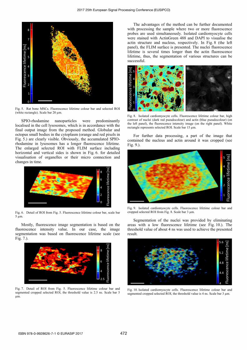
Fig. 5. Rat bone MSCs. Fluorescence lifetime colour bar and selected ROI

(white rectangle). Scale bar 20 µm.

SPIO-rhodamine nanoparticles were predominantly localised in the cell lysosomes, which is in accordance with the final output image from the proposed method. Globular and octopus small bodies in the cytoplasm (orange and red pixels in Fig. 5.) are clearly visible. Obviously, the accumulated SPIO-rhodamine in lysosomes has a longer fluorescence lifetime. The enlarged selected ROI with FLIM surface including horizontal and vertical sides is shown in Fig. 6. for detailed visualisation of organelles or their micro connection and changes in time.

Fig. 6. Detail of ROI from Fig. 5. Fluorescence lifetime colour bar, scale bar

5 µm.

Mostly, fluorescence image segmentation is based on the fluorescence intensity value. In our case, the image segmentation was based on fluorescence lifetime scale (see Fig. 7.).

Fig. 7. Detail of ROI from Fig. 5. Fluorescence lifetime colour bar and

segmented cropped selected ROI, the threshold value is 2.5 ns. Scale bar 5

µm.

The advantages of the method can be further documented with processing the sample where two or more fluorescence probes are used simultaneously. Isolated cardiomyocyte cells were stained with ActinGreen 488 and DAPI to visualise the actin structure and nucleus, respectively. In Fig. 8 (the left panel), the FLIM surface is presented. The nuclei fluorescence lifetime is several times longer than the actin fluorescence lifetime, thus, the segmentation of various structures can be successful.

Fig. 8. Isolated cardiomyocyte cells. Fluorescence lifetime colour bar, high

contrast of nuclei (dark red pseudocolour) and actin (blue pseudocolour) (on the left panel), the fluorescence intensity image (on the right panel). White

rectangle represents selected ROI. Scale bar 15 µm.

For further data processing, a part of the image that contained the nucleus and actin around it was cropped (see Fig. 9.).

Fig. 9. Isolated cardiomyocyte cells. Fluorescence lifetime colour bar and

cropped selected ROI from Fig. 8. Scale bar 3 µm.

Segmentation of the nuclei was provided by eliminating areas with a low fluorescence lifetime (see Fig. 10.). The threshold value of about 4 ns was used to achieve the presented result.

Fig. 10. Isolated cardiomyocyte cells. Fluorescence lifetime colour bar and

segmented cropped selected ROI, the threshold value is 4 ns. Scale bar 3 µm.

2017 25th European Signal Processing Conference (EUSIPCO)

ISBN 978-0-9928626-7-1 © EURASIP 2017 472

The rendering surfaces of the segmented structures are presented in Fig. 11. A threshold value of 2 ns was used and thus actin was segmented in the image. Then, the nucleus was segmented with a threshold value of 4 ns. Both structures were rendered as isosurfaces in green and blue colour.

Fig. 11. Isolated cardiomyocyte cells. Fluorescence lifetime colour bar and segmented cropped selected ROI, the threshold value is 2 ns (green surface)

and 4 ns (blue surface). Scale bar 3 µm.

IV. DISCUSSION

The scanning of a lifetime in different points of small biological samples has become a technical and economic reality for academic labs in recent years. The primary result after our 3-D confocal scanning of cells is a three-dimensional data array that represents the pixels in the two-dimensional scan (confocal layers), each pixel containing a value of fluorescence intensity in a large number of time intervals (time channels) after the excitation pulse. The fluorescence demonstrates an exponential decrease over the course of a few nanoseconds.

Transformation of the exponential curve or lifetime values to the visual pseudo colour 3D map is not a standard function of the confocal microscope, but it was the main aim of our work. The software utility was created and tested, and the first evaluation of the transformation of lifetime data to the 3D image was made on data from adhesive cells (MSCs with SPIO-rhodamine nanoparticles inside the cells). The next test was made on neonatal cardiomyocyte (where nuclei and cytoskeleton display different lifetimes). The last evaluation was made on thermosensitive nanoparticles (fluorescence with lifetime affected by temperature).

The first evaluation shows the great advantages of a clear resolution of lysosomes in MSCs (see Fig. 5.), with excellent results in 3D visualisation visible also for the nuclei and actin structures of cardiomyocytes (Fig. 8.). The second evaluation on thermosensitive particles (data not shown), also showed good spatial resolution of the methods; small clusters with different temperatures (mitochondria in specific biological phases, or heating of some region after infrared pulses, for example) can be precisely visualised and segmented by our software.

Our software can also bring new possibilities for all practical applications of FLIM in subcellular thermometry [12], pH quantification in biological objects [17], and gas concentration in microenvironments and inside the cells [18].

REFERENCES

[1] V. Cmiel, F. Mravec, T. Halasova, J. Sekora, and I. Provaznik, “Emission properties of potential-responsive probe di-4-ANEPPS,” Analysis of Biomedical Signals and Images, vol. 20, pp. 359–363, 2010.

[2] V. Cmiel, J. Odstrcilik, O. Svoboda, L. Baiazitova, and I. Provaznik, “Method for adult cardiomyocytes long-term viability monitoring using confocal microscopy techniques,” Computing in Cardiology Conference (CinC), 2015, pp. 961–964.

[3] L. Baiazitova, V. Cmiel, J. Pala, and I. Provaznik, “Simplified time resolved observation of cardiomyocytes by TimeGate function of hybrid detectors and pulsed white light laser,” International Microscopy Congress, 2014, pp. 1378–1379.

[4] Z. Burdikova, Z. Svindrych, J. Pala, C.D. Hickey, M.G. Wilkinson, J. Panek, M.A.E. Auty, A. Periasamy, and J.J. Sheehan, “Measurement of pH micro-heterogeneity in natural cheese matrices by fluorescence lifetime imaging,” Frontiers in Microbiology, vol. 6, pp. 82–88, 2015.

[5] K. Okabe, N. Inada, C. Gota, Y. Harada, T. Funatsu, and S. Uchiyama, “Intracellular temperature mapping with a fluorescent polymeric thermometer and fluorescence lifetime imaging microscopy,” Nature Communications, vol. 3, 705, 2012, pp. 1–9.

[6] J.A. Levitt, M.K. Kuimova, G. Yahioglu, P. Chung, K. Suhling, and D. Phillips, “Membrane-bound molecular rotors measure viscosity in live cells via fluorescence lifetime imaging,” The Journal of Physical Chemistry, vol. 113, pp. 11634–11642, 2009.

[7] G. Holst and B. Grunwald, “Luminescence lifetime imaging with transparent oxygen optodes,” Sensors and Actuators B: Chemical, vol. 74, pp. 78–90, 2001.

[8] S. Vira, E. Mekhedov, G. Humphrey, and P.S. Blank, “Fluorescent-labeled antibodies: Balancing functionality and degree of labeling,” Analytical Biochemistry, vol. 402, pp. 146–150, 2010.

[9] D. Egger, R. Bolten, C. Rahner, and K. Bienz, “Fluorochrome-labeled RNA as a sensitive, strand-specific probe for direct fluorescence in situ hybridization,” Histochemistry and Cell Biology, vol. 111, pp. 319–324, 1999.

[10] R.Y. Tsien, “Fluorescent and photochemical probes of dynamic biochemical signals inside living cells,” ACS Symposium Series, vol. 538, pp. 130–146, 1993.

[11] M. Klabusay, J. Skopalik, S. Erceg, and A. Hrdlička, “Aequorin as intracellular Ca2+ indicator incorporated in follicular lymphoma cells by hypoosmotic shock treatment,” Folia Biologica, vol. 61, pp. 134–139, 2015.

[12] G.L. Scott and H.C. Longuet-Higgins, “Feature grouping by ‘relocalisation’ of eigenvectors of the proximity matrix,” European Conference on Computer Vision, pp. 103–108, September 1990.

[13] P. Perona, and W. Freeman, “A factorization approach to grouping,” European Conference on Computer Vision, pp. 655–670, June 1998.

[14] J. Shi and J. Malik, “Normalized cuts and image segmentation,” IEEE Transactions on Pattern Analysis and Machine Intelligence, vol. 22, pp. 888–905, August 2000.

[15] A.P. Dempster, N.M. Laird, and D.B. Rubin, “Maximum likelihood from incomplete data via the EM algorithm,” Journal of the Royal Statistical Society. Series B (methodological), vol. 39, pp. 1–38, 1977.

[16] L. Shang, F. Stockmar, N. Azadfar, and G.U. Nienhaus, “Intracellular thermometry by using fluorescent gold nanoclusters,” Angewandte Chemie International Edition, vol. 52, pp. 11154–11157, 2013.

[17] G. Hidalgo, A. Burns, E. Herz, A.G. Hay, P.L. Houston, U. Wiesner, and L.W. Lion, “Functional tomographic fluorescence imaging of pH microenvironments in microbial biofilms by use of silica nanoparticle sensors,” Applied and Environmental Microbiology, vol. 75, pp. 7426–7435, 2009.

[18] R.I. Dmitriev, A.V. Zhdanov, G. Jasionek, and D.B. Papkovsky, “Assessment of cellular oxygen gradients with a panel of phosphorescent oxygen-sensitive probes,” Analytical Chemistry, vol. 84, pp. 2930–2938, 2012.

2017 25th European Signal Processing Conference (EUSIPCO)

ISBN 978-0-9928626-7-1 © EURASIP 2017 473