three-axis stabilized earth orbiting spacecraft simulator

American Institute of Aeronautics and Astronautics

1

Three-Axis Stabilized Earth Orbiting Spacecraft Simulator

A Senior Project

presented to

the Faculty of the Aerospace Engineering Department

California Polytechnic State University, San Luis Obispo

In Partial Fulfillment

of the Requirements for the Degree

Bachelor of Science

by

Alan F. Ma and Nikola N. Dominikovic

October, 2012

© 2012 Alan F. Ma and Nikola N. Dominikovic


2

Three-Axis Stabilized Earth Orbiting Spacecraft Simulator

Alan F. Ma1 and Nikola N. Dominikovic

2

California Polytechnic State University, San Luis Obispo, California, 93407

This report details the method and results of the program created for simulating an

Earth orbiting spacecraft with control actuators and orbital perturbations. The control

actuators modeled are reaction thrusters, reaction/momentum wheels, and control moment

gyros (CMG). The perturbations modeled were gravity gradient, electromagnetic torques,

solar radiation pressure, gravity gradients, third-body effects, Earth oblateness and

atmospheric drag. This simulation allows for satellite control in all 6 degrees of freedom for

any Earth orbiting spacecraft. Assumptions include rigid body dynamics, no sensor noise,

constant spacecraft cross-sectional area, constant coefficient of drag and reflectivity,

ignoring the effects due to the moon, moment of inertia doesn’t change with a change in

mass, and reaction thrusters only produce torque. The results from test trials showed

reasonable numbers and system behavior.

Nomenclature = cross-sectional area of the spacecraft in the ram direction (m2) = cross-sectional area of the spacecraft in the sun (m

2)

a = semi-major axis (km) = acceleration vector due to solar radiation pressure (km·s-2

)

α = reciprocal of the semi-major axis (km-1

) = spacecraft angular acceleration (s-2

)

β = reaction wheel angle from z-axis

C = Stumpff function = coefficient of drag = coefficient of reflectivity = center of mass (m) = center of pressure (m) = dipole moment of the spacecraft (J·T-1

)

E = eccentric anomaly (rad)

e = eccentricity = drag force (N) = reaction thruster force vector (N)

f = Lagrange coefficient = gravitational constant (m3·kg

-1·s

-2

g = Lagrange coefficient = angular momentum (km2·s

-1) = spacecraft moment of inertia (kg·m

2) = CMG moment of inertia (kg·m

2) = reaction wheel moment of inertia of the i

th wheel (kg·m

2)

i = inclination (rad) ! = Julian day number at 0 hr UT (days)

j = current density (I·A-1

) = Julian Date (days) "# = proportional control gain in the x-direction

1 Undergraduate Student, Aerospace Engineering Department, 1 Grand Avenue San Luis Obispo, CA 93407

2 Undergraduate Student, Aerospace Engineering Department, 1 Grand Avenue San Luis Obispo, CA 93407


3

"$ = proportional control gain in the y-direction "% = proportional control gain in the z-direction "# = derivative control gain in the x-direction "$ = derivative control gain in the x-direction "% = derivative control gain in the x-direction

k = boltzman’s constant (m2·kg·s

-2·K

1) &! = variable relating the daily F10.7 solar activity to a weighted average &' = variable representing the daily effects of the atmospheric density distribution &( = variable accounting for the semiannual effects &) = variable accounting for the changing atmospheric density with a deviation of the daily F10.7 from F81 &* = variable representing the dependence on geomagnetic activity index

L = mean longitude (deg) +,+ = Magnetic latitude

M = mean anomaly (deg) - = Earth magnetic field (T) -. = mass of Earth (kg)

m = mass of spacecraft (kg)

Ω = right ascension of the ascending node (deg) / = argument of perigee/perihelion (deg)

ϖ = longitude of perihelion (deg) / = spacecraft angular velocity (s-1

) /0 = spacecraft angular acceleration (s-2

) / = CMG angular velocity (s-1

) /0 = CMG angular acceleration (s-2

) / = i

th reaction wheel angular velocity (s

-1) /0 = i

th reaction wheel angular acceleration (s

-2) = solar pressure (kN·m

-2) 1 = any of the six orbital elements 234#56 = transformation matrix from perifocal to geocentric equatorial coordinate frame 78 = command quaternion vector 7. = error quaternion vector 7 = spacecraft quaternion vector 9 = reaction wheel coordinate transformation matrix :;<6 = position vector in geocentric equatorial coordinate frame (km) :;<#5 = position vector in perifocal coordinate frame (km)

r = position vector (km)

r0 = initial position vector (km) =/ = position vector from the satellite to the sun (km) =?/) = position vector of the third body relative to the Earth (km) =/) = position vector of the third body relative to the satellite (km) =@?/ = acceleration vector of the satellite relative to Earth (km·s-2

) A = density (kg·m-3

) A = night-time density profile (kg·m-3

)

S = Stumpff function

T = transformation matrix from ECI to ECEF B! = number of Julian centuries between J2000 and the date in question B = drag torque (N·m) BC = gravity gradient torque (N·m) B.# = disturbance torque (N·m) BD = magnetic torque (N·m) B = reaction thruster torque vector (N·m) B# = command torque in the x-direction (N·m) B$ = command torque in the y-direction (N·m)


4

B% = command torque in the z-direction (N·m) ∆F = change in time (s)

θ = true anomaly (rad) G = Greenwich sidereal time (rad)

µ = gravitational parameter (km3·s

-2) H) = gravitational parameter of the third body (km

3·s

-2)

V1,2 = voltage at points in the electron saturation region (V) I = velocity in ram direction (m·s-1

)

Vthe = thermal velocity (m·s-1

)

vr0 = initial radial component of velocity (km·s-1

)

v = velocity vector (km·s-1

)

v0 = initial velocity vector (km·s-1

) :J<6 = velocity vector in geocentric equatorial coordinate frame (km·s-1

) :J<#5 = velocity vector in perifocal coordinate frame (km·s-1

) K = universal anomaly (km1/2

)

I. Introduction

MATLAB program, 6 DOF Satellite Simulator, was created to simulate a three-axis stabilized spacecraft

orbiting the Earth. This two-body (or more) system simulates the effects of gravity gradient, solar radiation

pressure, atmospheric drag, Earth oblateness, third-body effects and electromagnetic torques. Gravity gradient

torques are caused when a spacecraft’s center of gravity is not aligned with its center of mass with respect to the

local vertical. Solar radiation pressure is the pressure due to electromagnetic radiation from the sun. The photons

from the sun’s beam transfer momentum from itself to the surfaces of a spacecraft that it comes in contact with thus

creating pressure. Solar radiation pressure is one of the more difficult perturbations to model. Its significance

changes with the altitude of the spacecraft; in low Earth orbit (LEO) it is almost negligible but in geosynchronous

orbit (GEO) it is one of the main sources of perturbations. Atmospheric drag is due to the spacecraft colliding with

particles in its orbit. It can cause both a torque and a force onto the spacecraft which will cause the spacecraft to both

rotate and translate. Atmospheric drag is only prevalent in low Earth orbit, so the assumption was made that all

atmospheric drag above an altitude of 1500 km is negligible and will be ignored. Earth oblateness is due to the Earth

not being a perfect sphere, thus gravity acts differently on a spacecraft depending on where the spacecraft is located

relative to the Earth. Third body perturbation is the gravitational attraction, in this case, of a satellite with, for

example, the sun where the Earth is the second body. And electromagnetic torques are due to residual magnetic

moments of the spacecraft. These residual moments can range anywhere from .1-20 A·m2. When a spacecraft’s

residual moment is not aligned with a local magnetic field, it experiences an electromagnetic torque that attempts to

align the magnet moment to the local field. The Earth’s magnetic field is complex, asymmetric and varies, however

for use in the ADCS design process, it is usually sufficient to model Earth’s magnetic field as a dipole and to

determine the maximum possible value of the magnetic torque for a spacecrafts altitude.1

Control actuators were modeled under these conditions using a set of and/or a combination of reaction thrusters,

reaction/momentum wheels, and control moment gyros (CMG). The program, in the form of a graphical user

interface (GUI) accepts user defined elements of the spacecraft (i.e. mass moment of inertia, classical orbital

elements, control actuators, duration, etc.) to generate a mission profile that includes, but not limited to disturbance

forces and moments on the spacecraft, performance of the control actuators, and orbital profile.

The simulation for a six degree of freedom satellite requires a lot of different information for accuracy; from the

control method and the control type to the orbital propagator and the disturbance modeling, with each method being

dependent on the other. The reason behind the centralization of all these methods is to simplify and more

importantly, quicken the design process of an Earth orbiting satellite. The goal of this program, 6 DOF Satellite

Simulator, is to achieve exactly that.

II. Orbital Determination

Before calculating the position of a spacecraft relative to the Earth, a time system was established using Julian

Date (JD). JD is the continuous count of the number of days since Greenwich noon (12:00 UT) on January 1, 4712.

It is also the universally adopted solution for astronomical problems.2 JD was used due to its simplicity of using

continuous count of days as opposed to dealing with months, days, hours, seconds, and minutes. JD was obtained by

using the following equations,3

A


5

! L 367P Q RSTT= UVW$XYZ[[\]^_`a bc* d e RSTT= \(VfDg b e h e 1,721,013.5 (1)

L ! e p(* (2)

where J0 is the Julian day number at 0 hr UT in days, y is the year, m is the month, d is the day, floor is the

MATLAB command that rounds to negative infinity, UT is universal time in hours, and JD is Julian Date in days.

After calculating for JD, planetary ephemeris was obtained with the planetary orbital elements and their centennial

rates found in Table 8.1 in Curtis.3 The following equations were used to calculate the planetary orbital elements,

B! L qrs(,*f',f*f)t,f(f (3)

1 L 1! e 10 B! (4)

L uHv1 Q w(x (5)

/ L y Q z (6)

- L Q y (7)

where T0 is the number of Julian centuries between J2000 and the date in question, Q is any one of the six planetary

orbital elements in Table 8.1 of Curtis, h is the angular momentum in km2·s

-1, µ is the gravitational parameter of the

sun of 1.327 × 1011

km3·s

-2, a is the semi-major axis in km, e is the eccentricity, ω is the argument of perihelion in

degrees, ϖ is the longitude of perihelion in degrees, Ω is the right ascension of the ascending node (RAAN) in

degrees, M is the mean anomaly in degrees, and L is the mean longitude in degrees. It should be noted that all

angular quantities were adjusted to lie between 0° and 360°. With eccentricity and mean anomaly, the eccentric

anomaly and true anomaly were calculated with the following equations from Curtis,3

| L - e w 2⁄ v- x - Q w 2⁄ v- x + (8)

Rv|x L | Q w sin | Q - (9)

Rv|x L 1 Q w cos | (10)

=FT L Rv|x Rv|x⁄ (11)

|X' L | Q =FT (12)

G L 2 tans' a``^ (13)

where E is the eccentric anomaly in radians, M is the mean anomaly in radians, θ is true anomaly in radians. It

should be noted that Eqs. (9-12) are in an iterative loop to solve for E, where the loop breaks once ratioi, or the

tolerance, of 10-6

is reached. Equation (8) was used as an initial estimate for the eccentric anomaly to input into the

iterative loop. Once the approximate eccentric anomaly (where the accuracy was chosen by the tolerance) is solved

for, it is then used in Eq. (13) to obtain the true anomaly. With all of the planetary orbital elements, the state vectors

of the planets were calculated using the following equations,3

:;<#5 L a ''X. Ucos Gsin G0 d (14)


6

:J<#5 L U Q sin Gw e cos G0 d (15)

234#56 L Q sin z cos sin / e cos z cos / Q sin z cos cos / Q cos z sin / sin z sin cos z cos sin / e sin z cos / cos z cos cos / Q sin z sin / Q cos z sin sin sin / sin cos / cos (16)

:;<6 L 234#56:;<#5 (17)

:J<6 L 234#56:J<#5 (18)

where :;<#5 is the position vector in the perifocal frame in km, :J<#5 is the velocity vector in the perifocal frame in

km·s-1

, 234#56 is the transformation matrix from perifocal to geocentric equatorial frame, i is the inclination in

radians, z is RAAN in radians, ω is the argument of perigee/perihelion in radians, :;<6 is the position vector in the

geocentric equatorial frame in km, and :J<6 is the velocity vector in the geocentric equatorial frame in km·s-1

. It

should be noted that to obtain the state vectors in a heliocentric frame for planetary ephemeris, a H of 1.327 × 1011

km3·s

-2 was used and ω is the argument of perihelion. Equations (14-18) were also used to obtain the state vectors for

a satellite in orbit around the Earth, where a H of 398600 km3·s

-2 was used and ω is the argument of perigee. To

obtain the state vectors of a satellite in orbit after a change in time and ignoring orbital perturbations, universal

variables with Stumpff functions were used. First, the universal anomaly, K, was obtained with the following

equations in an iterative loop,3

=! L u;! · ;! (19)

! L uJ! · J! (20)

! L ;·J (21)

L ( e a (22)

K! L √H||∆F (23)

L K( (24)

vx L ¡¢¡£

√%s¤ √%¥√%¦§ v 0x¤¨ √s%s√s%¥√s%¦§ v 0x 't v L 0x

+ (25)

vx L ¡¢¡£

's √%% v 0x ¨ √s%s's% v 0x '( v L 0x

+ (26)

RvKx L ©√ K(vx e v1 Q =!xK)vx e =!K Q √H∆F (27)

RªvKx L ©√ K21 Q K(vx4 e v1 Q =!xK(vx e =! (28)

=FT L RvKx RvKx⁄ (29)


7

KX' L K Q =FT (30)

where r0 is the initial position in km, r0 is the initial position vector in km, v0 is the initial velocity in km·s-1

, v0 is the

initial velocity vector in km·s-1

, vr0 is the initial radial component of velocity in km·s-1

, α is the reciprocal of the

semi-major axis in km-1

, χ is the universal anomaly in km1/2

, S and C are Stumpff functions. It should be noted that

the above equations are in a loop similar to Eqs. (8-12). Once χ is obtained, it is then used in the following equations

to calculate for the new state vectors,

R L 1 Q «a vK(x (31)

¬ L ∆F Q '√ K)vK(x (32)

R0 L √ 2K)vK(x Q K4 (33)

¬0 L 1 Q «a vK(x (34)

; L R;! e ¬J! (35)

J L R0;! e ¬0J! (36)

where f and g are Lagrange coefficients in terms of the universal anomaly, ∆F is the change in time in seconds, r is

the new position vector in km, and v is the new velocity vector in km·s-1

. It should be noted that ∆F needs to be in

small intervals relative to the period of the orbit, otherwise there would be a significant inaccuracy in the new state

vectors. To propagate the orbit of a satellite accounting for perturbations, Encke’s formulation was used. In Encke’s

method, the orbit is propagated by integrating the the differences between the osculating and the perturbed orbit.

This process continues until the tolerance of about 1% is met, where the osculating orbit is re-initialized.4

III. Orbital Perturbations

A. Atmospheric Drag

Atmospheric drag is the first perturbation that the spacecraft will undergo The simplified equation to the

atmospheric drag force and torque are given by Space Mission Engineering: The New SMAD and are1

B L '( AI( # Q #0 % Q % (37)

L '( AI( (38)

where Ta and Fa is the atmospheric drag torque and force, respectively, ρ is the atmospheric density in kg·m-3

, Cd is

the drag coefficient of the spacecraft, Ar is the area of the spacecraft in the ram direction in m2 and Vr is the velocity

in the ram direction in km·s-1

. cpx and cpz are the center of pressure in the x and z direction respectively and, cmx and

cmz are the center of mass in the x and z direction respectively. It should be noted that the cp and the cm need to be

in terms of the Local-Vertical Local-Horizontal (LVLH) reference frame and not the body frame. A lot of these

parameters change as the spacecraft rotates so it is assumed that transient rotations are not vastly different than the

desired controlled attitude and is ignored. Also ignored are any small deviations from the desired controlled attitude

due to controller type. So the only parameters that would be inputted are those at the controlled attitude.

To model the atmospheric density, the Russian GOST model was used. This model was constructed from

observations of the orbital motion of Russian Cosmos satellites. The density, A in kg·m-3

, was calculated with the

following equation,4

A L A&!&'&(&)&* (39)


8

where A is the night-time density profile in kg·m-3

, &! relates the daily F10.7 solar activity to a weighted average, &'

represents the daily effects of the atmospheric density distribution, &( accounts for the semiannual effects, &)

accounts for the changing atmospheric density with a deviation of the daily F10.7 from F81, and &* represents the

dependence on geomagnetic activity index. The equations and tables used for this model can be found in Appendix

B.2 in Fundamentals of Astrodynamics and Applications.4 This model is only valid for an altitude range of 120-1500

km.

B. Electromagnetic Torques

The second orbital perturbation is the electromagnetic torques. Electromagnetic forces are very small and

complicated and are only notable on spacecraft with long conductive tether systems. For this reason electromagnetic

forces will be ignored. The simplified equation for electromagnetic torques is given by1

BD L \§ ,b (40)

where Tm is the electromagnetic torque, D is the dipole moment of the spacecraft, M is the magnetic field of Earth, r

is the distance of the spacecraft to the center of Earth, and λ is a unitless function of the magnetic latitude that ranges

from 1 at the magnetic equator and 2 at the magnetic poles.

C. Solar Radiation Pressure

To correctly and accurately model SRP, a precise location of the Sun, spacecraft attitude, time-varying cross-

sectional area, and time-varying coefficient of reflectivity need to be known. In this case, the cross-sectional area

and coefficient of reflectivity are assumed to be constant due to the complexity of accounting for those variables.

Eclipses are accounted for in the spacecrafts orbit to determine when SRP is on or off. To calculate SRP, the

following equation was used4

L Q ®¯©©°¯±²D ¯³´/¯±²µ¯³´/¯±²µ (41)

where is the acceleration due to solar radiation pressure in km·s-2

, is the solar pressure of 4.57×10-9

kN·m-2

where the solar flux is 1367 W·m-2

, is the coefficient of reflectivity, is the cross-sectional area of the

spacecraft in the sun in m2, m is the mass of the spacecraft in kg, and =/ is the position vector from the satellite

to the sun in km. To determine if the satellite is in an eclipse, Algorithm 34 from Fundamentals of Astrodynamics

and Applications4 was used. It uses simple geometry by examining the satellite’s vertical and horizontal distances

from the Earth-Sun line. It was assumed that if the satellite was in either the penumbra or umbra region, it is in a

total eclipse.

D. Third Body

Similarly to SRP the effects of third body perturbations on a satellite are, more or less significant with respect to

the altitude of a satellite. In this case, third body perturbations due to the Moon are ignored, the mass of the satellite

is negligible, and all planets up to Neptune (including the Sun) are considered. To calculate this acceleration, the

following equation was used4

=@?/ L QH) ¶¯³´/§ ³´/§§ Q ?/§?/§§ · (42)

where =@?/ is the acceleration vector of the satellite relative to Earth in km·s-2

, H) is the gravitational parameter of

the third body in km3·s

-2, =/) is the position vector of the third body relative to the satellite in km, and =?/) is the

position vector of the third body relative to the Earth in km. Equation 42 is used to find the third body acceleration

of each individual planet, the sum is taken to obtain the total acceleration.


9

E. Earth Oblateness

Since the Earth is not a perfect sphere, perturbing accelerations due to the Earth varies with where the spacecraft

is located at. Using the Legendre functions in Table 8-2, the gravitational coefficients in Table D-1/2, and equations

from page 548 from Fundamentals of Astrodynamics and Applications4, the accelerations were modeled. Zonal,

sectorial, and tesseral harmonics are accounted for from a Legendre function of P2,0 (J2) to P4,4. Zonal harmonics,

such as J2 accounts for most of the gravitational effects due to oblateness; it represents bands of latitude. Sectorial

harmonics and tesseral harmonics represents bands of longitude and specific regions of the Earth (in a checkered

pattern), respectively.4 To calculate the acceleration, the position and velocity vector of the satellite had to be

converted from an Earth-Centered Inertial (ECI) coordinate frame to an Earth-Centered, Earth-Fixed (ECEF)

coordinate frame using the following equations,4,5

B L T¸vGx ¸¹vGx 0Q¸¹vGx T¸vGx 00 0 1 (43)

B0 L Q/º¸¹vGx /º T¸vGx 0Q/º T¸vGx Q/º¸¹vGx 00 0 0 (44)

B@ L »Q/º( T¸vGx Q/º( ¸¹vGx 0/º(¸¹vGx Q/º( T¸vGx 00 0 0¼ (45)

=ºº½ L B=º¾ (46)

ºº½ L Bº¾ e B0 =º¾ (47)

ºº½ L Bº¾ e 2B0 º¾ e B@ =º¾ (48)

where T is the transformation matrix from ECI to ECEF, G is the Greenwich sidereal time in rad, /ºis the inertial

rotation rate of the Earth of 7.2921×10-5

in rad/s.

F. Gravity Gradient

The most general form of the equation in an inverse square gravity field is given by6

BC L )¿ = (49)

where Tg is the gravity torque, G is the gravitational constant, Me is the mass of the Earth, r is the distant between the

center of the earth and the center of the spacecraft. I is the moment of the inertia in the LVLH reference frame and

might not be a principle inertia matrix.

IV. Control Actuators Dynamics

A. Reaction/Momentum Wheels

The first type of control system that can be modeled onto the spacecraft are reaction or momentum wheels. The

difference between a reaction wheel and a momentum wheel is that a reaction wheel only acts to remove

disturbances from the spacecraft while a momentum wheel can hold a significant amount of momentum to make it

harder for disturbances to affect the system while also removing the disturbances. Physically they are identical, only

difference being momentum wheels are typically larger. The program allows you to model both, but for now they

will be referred to as only reaction wheels.

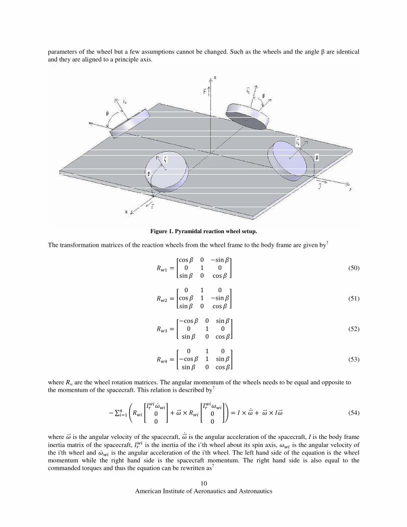
The first step is to determine how the reaction wheels will be placed in the spacecraft. A common setup for

reaction wheels is a four wheel pyramidal setup as seen in Fig. 1, where all four wheels are in the same plane but are

angled at a specific β angle. This is the setup that the program uses. The β angle can be changed as well as all the


10

parameters of the wheel but a few assumptions cannot be changed. Such as the wheels and the angle β are identical

and they are aligned to a principle axis.

Figure 1. Pyramidal reaction wheel setup.

The transformation matrices of the reaction wheels from the wheel frame to the body frame are given by7

9' L cos À 0 Qsin À0 1 0sin À 0 cos À (50)

9( L 0 1 0cos À 1 Qsin Àsin À 0 cos À (51)

9) L Qcos À 0 sin À0 1 0sin À 0 cos À (52)

9* L 0 1 0Qcos À 1 sin Àsin À 0 cos À (53)

where Rw are the wheel rotation matrices. The angular momentum of the wheels needs to be equal and opposite to

the momentum of the spacecraft. This relation is described by7

Q ∑ Â9 /0 00 e / 9 /00 Ã*Ä' L /0 e / / (54)

where / is the angular velocity of the spacecraft, /0 is the angular acceleration of the spacecraft, I is the body frame

inertia matrix of the spacecraft, is the inertia of the i’th wheel about its spin axis, / is the angular velocity of

the i'th wheel and /0 is the angular acceleration of the i'th wheel. The left hand side of the equation is the wheel

momentum while the right hand side is the spacecraft momentum. The right hand side is also equal to the

commanded torques and thus the equation can be rewritten as7


11

Q ∑ Â9 /0 00 e / 9 /00 Ã*Ä' L »B#B$B%¼ (55)

where B#, B$ and B% are the command torques in the x, y and z directions. The angular velocity of the wheel, / , is

a known quantity that can be directly measured onboard and therefore can be subtracted from the commanded torque

to obtain7

»B#B$B%¼ e ∑ Â/ 9 /00 Ã*Ä' L Q ∑ Â9 /0 00 Ã*Ä' (56)

Now, we can redefine the left hand side as ÅBÆ# BÆ$ BÆ%Ç, and 2'/0 ' (/0 ( )/0 ) */0 *4 as 2B' B( B) B*4. Using Eqs. (50-53) we can rewrite and expand Eq. (56) as

7

»BÆ#BÆ$BÆ%¼ L cos À 00 cos Àsin À sin À Q cos À 00 Q cos Àsin À sin À a§È

(57)

The reaction wheel torques are desired, but the matrix relating the desired torques to the reaction wheel torques is

not square and therefore non-invertible. Sidi8 describes that one possible way to distribute the torques between the

four reaction wheels is to define ÅBÆ# cos À⁄ BÆ$ cos À⁄ BÆ% sin À⁄ Ças ÅBÆ# BÆ$ BÆ%Ç

so that7

»BÆ#BÆ$BÆ%¼ L 1 00 11 1 Q1 00 Q11 1 a§È

L a§È

(58)

The matrix Aw is still not square but by taking the right pseudo-inverse of Aw the equation becomes7

a§È L '( ' ! ' (⁄ ! ' ' (⁄s' ! ' (⁄! s' ' (⁄ »BÆ#BÆ$BÆ%

¼ (59)

Now we have the equation that obtains the torques on all four wheels given the command torques of the spacecraft.

The next step is to determine how to control the spacecraft and how to obtain the command torques. To control the

spacecraft a quaternion error controller was used because it does not suffer from gimbal locks as would an Euler

control method and performs well with large commanded angles. The quaternion error is defined as8

7. L É ÊËÈ ÊË§sÊË§ ÊËÈ sÊËa ÊË` ÊË` ÊËaÊËa sÊË`sÊË` sÊËa ÊËÈ ÊË§sÊË§ ÊËÈÌ ÉsÊ¯`sÊ¯asÊ¯§Ê¯È

Ì (60)

where qe is the quaternion error matrix, qc is the commanded quaternion vector and qs is the spacecraft quaternion

vector. Finally the control law to obtain the command torques is given by8

B#B$B%L Q2"#7'.7*. e "#L Q2"$7(.7*. e "$7L Q2"%7).7*. e "%= (61)

where K are control gains and, p, q and r are the body roll rates in x, y and z direction, respectively. Finally we have

the dynamics of the spacecraft where we want to find the acceleration of the spacecraft, which is used to update the


12

location of the spacecraft, the spacecraft quaternion, reaction wheel speed/saturation and etc. The spacecraft

acceleration equation come from Curtis and is given by3

L s' B.# Q ¥/ v/x¦ Q ∑ Â/ 9 /00 Ã Q ∑ Â9 00 Ã*Ä'*Ä' Í (62)

where is the angular acceleration of the spacecraft, B.# are the external torques (in body frame) and is the

acceleration of the i’th wheel. From the acceleration the body rates can easily be found by taking a derivative.

B. Control Moment Gyros

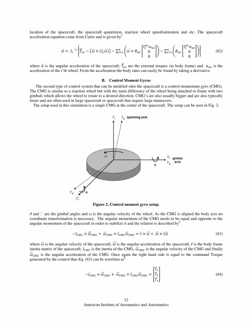
The second type of control system that can be modeled onto the spacecraft is a control momentum gyro (CMG).

The CMG is similar to a reaction wheel but with the main difference of the wheel being attached to frame with two

gimbals which allows the wheel to rotate to a desired direction. CMG’s are also usually bigger and are also typically

faster and are often used in large spacecraft or spacecraft that require large maneuvers.

The setup used in this simulation is a single CMG at the center of the spacecraft. The setup can be seen in Fig. 2.

Figure 2. Control moment gyro setup.

θ and ϖ are the gimbal angles and ω is the angular velocity of the wheel. As the CMG is aligned the body axis no

coordinate transformation is necessary. The angular momentum of the CMG needs to be equal and opposite to the

angular momentum of the spacecraft in order to stabilize it and the relation is described by8

Q /0 e / / L /0 e / / (63)

where / is the angular velocity of the spacecraft, /0 is the angular acceleration of the spacecraft, I is the body frame

inertia matrix of the spacecraft, is the inertia of the CMG, / is the angular velocity of the CMG and finally /0 is the angular acceleration of the CMG. Once again the right hand side is equal to the command Torque

generated by the control thus Eq. (63) can be rewritten as8

Q /0 e / / L »B#B$B%¼ (64)


13

where B#, B$ and B% are the command torques in the x, y and z directions. The angular velocity of the wheel, /,

is a known quantity that can be directly measured onboard and therefore can be subtracted from the commanded

torque to obtain8

Q /0 L »B#B$B%¼ Q / / (65)

The right hand side can be rewritten as ÅBÆ# BÆ$ BÆ%Ç while the left hand side is simply the torque of the CMG so

the equation becomes8

»BÆ#BÆ$BÆ%¼ L Q »B#B$B%

¼

(66)

Where 2B# B$ B%4 is the torque of the CMG. Now we have the equation that obtains the torque for the CMG

given the command torques of the spacecraft. The torque of the CMG can be rewritten to include the gimbal angles

and the torque of the actual wheel.3

»BÆ#BÆ$BÆ%¼ L Q sin G cos Îsin G sin Îcos G cos Î BÏ (67)

where BÏ is the torque of the wheel in the CMG system. The CMG uses the same controller and quaternion

feedback system as the reaction wheels as seen in Eq. (60) and (61). Finally the dynamics of the spacecraft where

we want to find the acceleration of the spacecraft can be known, which is used to update the location of the

spacecraft, the spacecraft quaternion, wheel speed/saturation and etc. The spacecraft acceleration equation come

from Curtis and is given by3

L s'ÐB.# Q ¥/ v/x¦ Q /0 Q / /Ñ (68)

where is the angular acceleration of the spacecraft and B.# are the external torques (in body frame). From the

acceleration the body rates can be found by taking a derivative.

C. Reaction Thrusters

The final type of control system is reaction thrusters which can provide a torque and force onto the spacecraft

when fired. But, the force due to the thrusters is ignored for simplicity. The torque is dependent on the location and

direction of the thruster relative to the center of mass of the spacecraft. Thrusters are common on a lot of spacecraft

and are also used in conjunction with reaction wheels as well as CMGs for dumping excess momentum in the

wheels. The basic equation of the Torque generated by a thruster is given by3

B L = (69)

where B is the torque generated by the thruster, = is the position vector of the thruster relative to the center of

mass and is the force generated by the thruster. The force of the thruster and the position vector are

assumed to be fixed quantities. The simulation allows for up to 12 different thrusters all with different locations

and thrust vectors. An algorithm was built to be able to find the torque generated by firing all combinations of

thrusters up to a total of six at a time. Which combination of thrusters that are fired is once again determined by the

quaternion control law seen in Eq. (61). The thruster combination that is closest to the command torque is chosen

and fired for the duration of the pulse time (which can be set by the user) before a new combination is chosen to

fire. The spacecraft acceleration equation for the spacecraft with thrusters is given by3


where is the angular acceleration of the spacecraft and

frame). From the acceleration the body rates can be found by

with thrusters and another type of control system (for momentum dumping, as an example), simply add the torque

generated by thrusters to Eq. (62) or (68

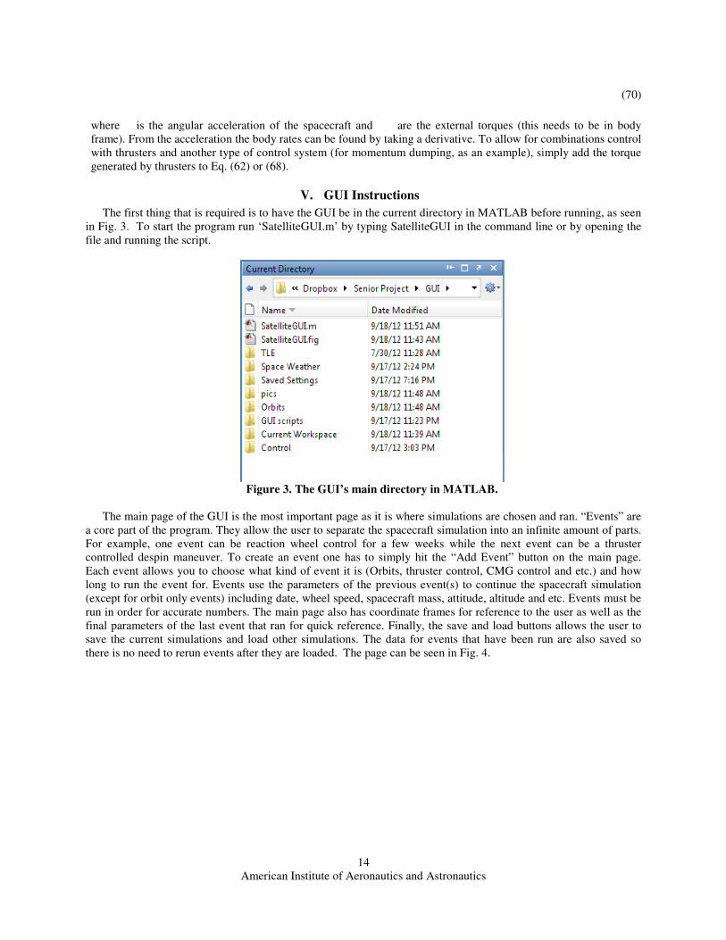
The first thing that is required is to have the GUI be in the current directory in MATLAB before running, as seen

in Fig. 3. To start the program run ‘SatelliteGUI.m’ by typing SatelliteGUI in the command line or by opening the

file and running the script.

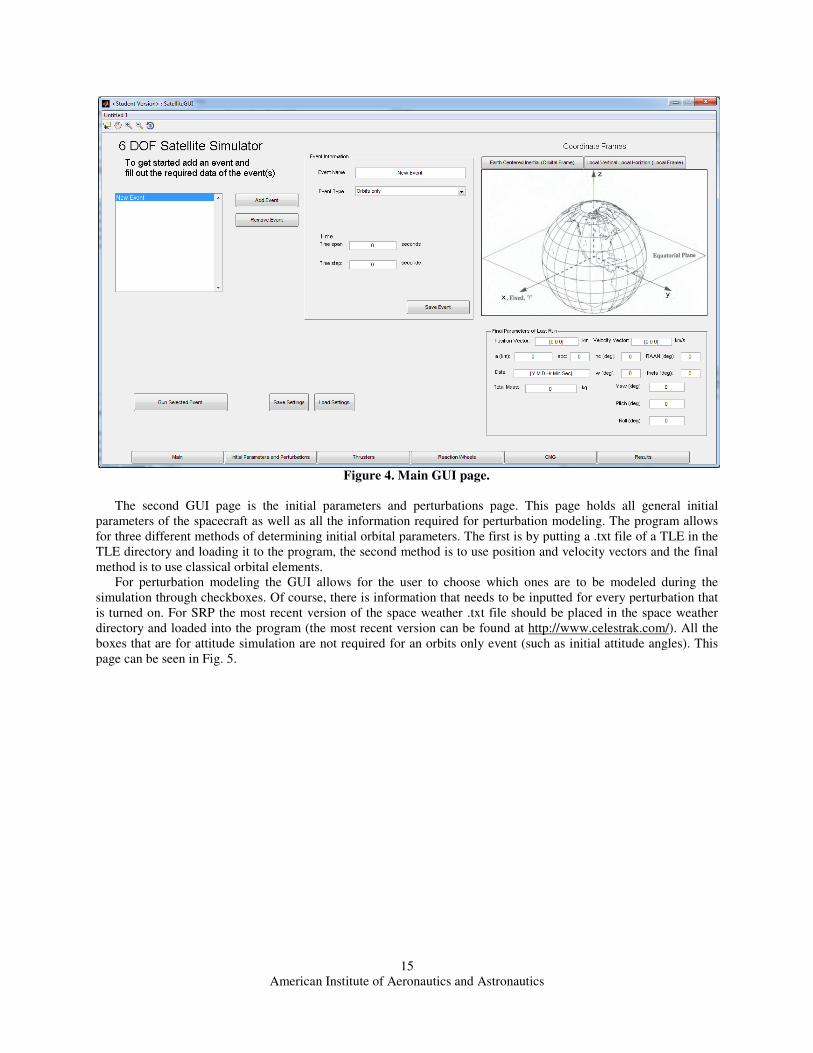
Figure

The main page of the GUI is the most important page as it is where simulations are chosen and ran.

a core part of the program. They allow

For example, one event can be reaction wheel control for a few weeks while the next event can be a thruster

controlled despin maneuver. To create an event one has to simply hit the “Add Event” button on the main page.

Each event allows you to choose what k

long to run the event for. Events use the parameters of the previous event(s) to continue the spacecraft simulation

(except for orbit only events) including date, wheel speed, spac

run in order for accurate numbers. The main page also has coordinate frames for reference to the user as well as the

final parameters of the last event that ran

save the current simulations and load other simulations. The data for events that have been run are also saved so

there is no need to rerun events after they are loaded.


14

is the angular acceleration of the spacecraft and are the external torques (this needs to be in body

frame). From the acceleration the body rates can be found by taking a derivative. To allow for combinations control


68).

V. GUI Instructions

to have the GUI be in the current directory in MATLAB before running, as seen

. To start the program run ‘SatelliteGUI.m’ by typing SatelliteGUI in the command line or by opening the

Figure 3. The GUI’s main directory in MATLAB.

is the most important page as it is where simulations are chosen and ran.

the user to separate the spacecraft simulation into an infinite amount of parts.

one event can be reaction wheel control for a few weeks while the next event can be a thruster


Each event allows you to choose what kind of event it is (Orbits, thruster control, CMG control and etc.) and how

. Events use the parameters of the previous event(s) to continue the spacecraft simulation

(except for orbit only events) including date, wheel speed, spacecraft mass, attitude, altitude and etc. E


that ran for quick reference. Finally, the save and load buttons allows the user to


there is no need to rerun events after they are loaded. The page can be seen in Fig. 4.

(70)

are the external torques (this needs to be in body

taking a derivative. To allow for combinations control


to have the GUI be in the current directory in MATLAB before running, as seen

. To start the program run ‘SatelliteGUI.m’ by typing SatelliteGUI in the command line or by opening the

is the most important page as it is where simulations are chosen and ran. “Events” are

separate the spacecraft simulation into an infinite amount of parts.

one event can be reaction wheel control for a few weeks while the next event can be a thruster


ind of event it is (Orbits, thruster control, CMG control and etc.) and how

. Events use the parameters of the previous event(s) to continue the spacecraft simulation

s, attitude, altitude and etc. Events must be


and load buttons allows the user to



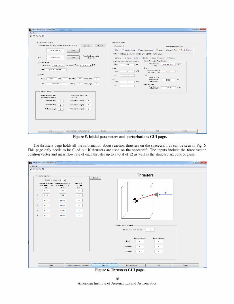
The second GUI page is the initial parameters and perturbations page.

parameters of the spacecraft as well as all the information required for perturbation modeling. The program allows

for three different methods of determining initial orbital parameters.

TLE directory and loading it to the program, the second method is to use position and velocity vectors and the final

method is to use classical orbital elements.

For perturbation modeling the GUI allows for the user to choose which ones are to be modeled

simulation through checkboxes. Of course, there is information that needs to be inputted for every perturbation that

is turned on. For SRP the most recent version of the space weather .txt file should be placed in the space weather

directory and loaded into the program (the most recent version can be found at

boxes that are for attitude simulation are not required for an orbits only event (such as initial

page can be seen in Fig. 5.


15

Figure 4. Main GUI page.

nitial parameters and perturbations page. This page holds all


for three different methods of determining initial orbital parameters. The first is by putting a .txt file of a TLE in the

LE directory and loading it to the program, the second method is to use position and velocity vectors and the final

method is to use classical orbital elements.

For perturbation modeling the GUI allows for the user to choose which ones are to be modeled

Of course, there is information that needs to be inputted for every perturbation that


loaded into the program (the most recent version can be found at http://www.celestrak.com/

boxes that are for attitude simulation are not required for an orbits only event (such as initial attitude angles)

holds all general initial


The first is by putting a .txt file of a TLE in the

LE directory and loading it to the program, the second method is to use position and velocity vectors and the final

For perturbation modeling the GUI allows for the user to choose which ones are to be modeled during the

Of course, there is information that needs to be inputted for every perturbation that


http://www.celestrak.com/). All the

attitude angles). This


Figure 5. Initial parameters and perturbations GUI page.

The thrusters page holds all the information about

This page only needs to be filled out if thru

position vector and mass flow rate of each thruster up to a total of 12


16

. Initial parameters and perturbations GUI page.

page holds all the information about reaction thrusters on the spacecraft, as can be seen in Fig

page only needs to be filled out if thrusters are used on the spacecraft. The inputs include the force vector,

position vector and mass flow rate of each thruster up to a total of 12 as well as the standard six control

Figure 6. Thrusters GUI page.

, as can be seen in Fig. 6.

sters are used on the spacecraft. The inputs include the force vector,

as well as the standard six control gains.


17

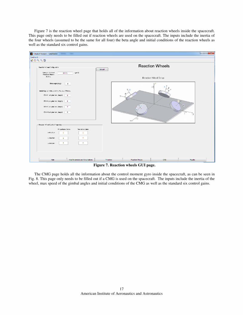
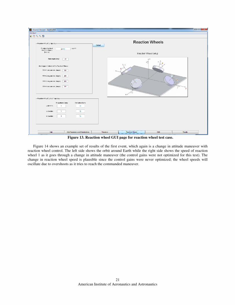
Figure 7 is the reaction wheel page that holds all of the information about reaction wheels inside the spacecraft.

This page only needs to be filled out if reaction wheels are used on the spacecraft. The inputs include the inertia of

the four wheels (assumed to be the same for all four) the beta angle and initial conditions of the reaction wheels as

well as the standard six control gains.

Figure 7. Reaction wheels GUI page.

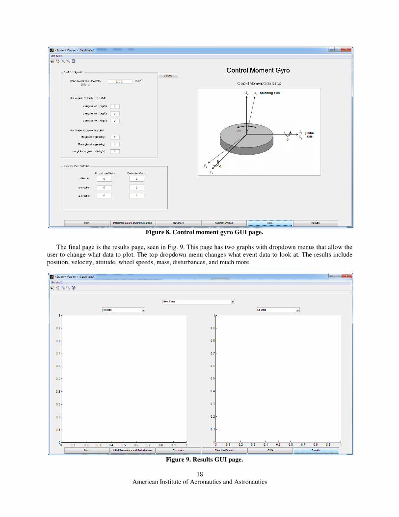
The CMG page holds all the information about the control moment gyro inside the spacecraft, as can be seen in

Fig. 8. This page only needs to be filled out if a CMG is used on the spacecraft. The inputs include the inertia of the

wheel, max speed of the gimbal angles and initial conditions of the CMG as well as the standard six control gains.


Figure

The final page is the results page, seen in Fig

user to change what data to plot. The top dropdown menu changes what event data to look at. The results include

position, velocity, attitude, wheel speeds, mass, disturbances, and much more.


18

Figure 8. Control moment gyro GUI page.

, seen in Fig. 9. This page has two graphs with dropdown menus that allow the


velocity, attitude, wheel speeds, mass, disturbances, and much more.

Figure 9. Results GUI page.

. This page has two graphs with dropdown menus that allow the



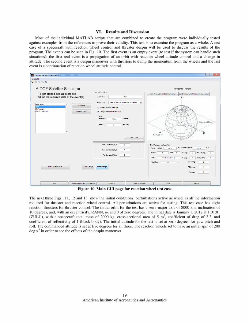
Most of the individual MATLAB scripts that are combined to create the program were individually tested

against examples from the references to prove their validity. This test is to examine the program as a whole.

case of a spacecraft with reaction wheel con

program. The events can be seen in Fig

situations); the first real event is a propagation of an orbit with reaction wheel attitude control

attitude. The second event is a despin maneuver with thrusters to

event is a continuation of reaction wheel attitude control.

Figure 10

The next three Figs., 11, 12 and 13, show the

required for thruster and reaction wheel control. All perturbations are active for testing.

reaction thrusters for thruster control. The initial orbit for the test

10 degrees, and, with an eccentricity, RANN,

(ZULU), with a spacecraft total mass of 2000 kg, cross

coefficient of reflectivity of 1 (black body).

roll. The commanded attitude is set at five degrees for all three. The reaction wheels set to have an initial spin of 200

deg·s-1

in order to see the effects of the despin maneuver.


19

VI. Results and Discussion


ferences to prove their validity. This test is to examine the program as a whole.

case of a spacecraft with reaction wheel control and thruster despin will be used to discuss the results of the

ig. 10. The first event is an empty event (to test if the system can handle such

is a propagation of an orbit with reaction wheel attitude control

event is a despin maneuver with thrusters to dump the momentum from the wheels and the last

event is a continuation of reaction wheel attitude control.

10. Main GUI page for reaction wheel test case.

, show the initial conditions, perturbations active as wheel as all the information

required for thruster and reaction wheel control. All perturbations are active for testing. This test case has

The initial orbit for the test has a semi-major axis of 8000 km, in

RANN, ω, and θ of zero degrees. The initial date is January 1, 2012 at 1:01:01

, with a spacecraft total mass of 2000 kg, cross-sectional area of 5 m2, coefficient of drag of 2.2, and

reflectivity of 1 (black body). The initial attitude for the test is set at zero degrees for yaw pitch and


e effects of the despin maneuver.


ferences to prove their validity. This test is to examine the program as a whole. A test

be used to discuss the results of the

The first event is an empty event (to test if the system can handle such

is a propagation of an orbit with reaction wheel attitude control and a change in

dump the momentum from the wheels and the last

s wheel as all the information

This test case has eight

major axis of 8000 km, inclination of

of zero degrees. The initial date is January 1, 2012 at 1:01:01

, coefficient of drag of 2.2, and

The initial attitude for the test is set at zero degrees for yaw pitch and



Figure 11. Initial parameters and perturbations GUI page for reaction wheel test case.

Figure 12. Thrusters GUI page for reaction wheel test case.


20

. Initial parameters and perturbations GUI page for reaction wheel test case.

. Thrusters GUI page for reaction wheel test case.

. Initial parameters and perturbations GUI page for reaction wheel test case.


Figure 13. Reaction wheel GUI page for reaction wheel test case.

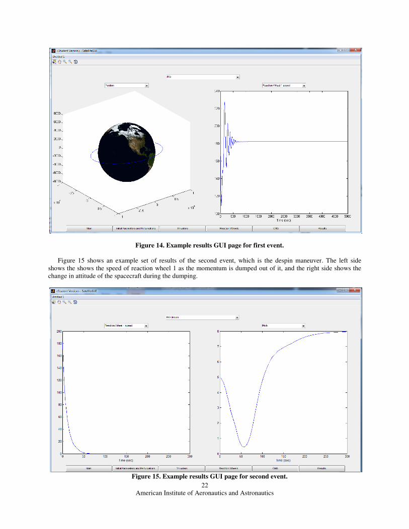
Figure 14 shows an example set of results of the first event

reaction wheel control. The left side shows the orbit around Earth while the right side shows the speed of reaction

wheel 1 as it goes through a change in attitude maneuver (the control gains were not optimized for this test).

change in reaction wheel speed is plausible since the control gains were never optimized; the wheel speeds will

oscillate due to overshoots as it tries to reach the com


21

. Reaction wheel GUI page for reaction wheel test case.

shows an example set of results of the first event, which again is a change in attitude maneuver with

. The left side shows the orbit around Earth while the right side shows the speed of reaction

a change in attitude maneuver (the control gains were not optimized for this test).


as it tries to reach the commanded maneuver.

, which again is a change in attitude maneuver with

. The left side shows the orbit around Earth while the right side shows the speed of reaction

a change in attitude maneuver (the control gains were not optimized for this test). The



Figure

Figure 15 shows an example set of results of the

shows the shows the speed of reaction wheel 1 as the momentum is dumped out of it, and the right side shows the

change in attitude of the spacecraft during the dumping.

Figure 15


22

Figure 14. Example results GUI page for first event.

shows an example set of results of the second event, which is the despin maneuver

of reaction wheel 1 as the momentum is dumped out of it, and the right side shows the

change in attitude of the spacecraft during the dumping.

15. Example results GUI page for second event.

, which is the despin maneuver. The left side

of reaction wheel 1 as the momentum is dumped out of it, and the right side shows the


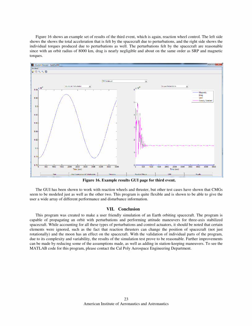
Figure 16 shows an example set of results of the third

shows the shows the total acceleration t

individual torques produced due to perturbations as well.

since with an orbit radius of 8000 km, drag is nearly negligible and about on the same order as SRP and magnetic

torques.

Figure

The GUI has been shown to work with

seem to be modeled just as well as the other two.

user a wide array of different performance and disturbance

This program was created to make a user friendly simulation of an Earth orbiting spacecraft. The program

capable of propagating an orbit with perturbations and performing attitude maneuvers

spacecraft. While accounting for all these types of perturbations and control actuators, it should be noted that certain

elements were ignored, such as the fact that reacti

rotationally) and the moon has an effect on the spacecraft.

due to its complexity and variability, the results of the simulation test

can be made by reducing some of the assumptions made, a

MATLAB code for this program, please contact the Cal Poly Aerospace Engineering Department.


23

shows an example set of results of the third event, which is again, reaction wheel control. The left side

shows the shows the total acceleration that is felt by the spacecraft due to perturbations, and the right side shows the

individual torques produced due to perturbations as well. The perturbations felt by the spacecraft are reasonable


Figure 16. Example results GUI page for third event.

has been shown to work with reaction wheels and thruster, but other test cases have shown that CMG

seem to be modeled just as well as the other two. This program is quite flexible and is shown to be able to give the

user a wide array of different performance and disturbance information.

VII. Conclusion

This program was created to make a user friendly simulation of an Earth orbiting spacecraft. The program

capable of propagating an orbit with perturbations and performing attitude maneuvers for three

While accounting for all these types of perturbations and control actuators, it should be noted that certain

elements were ignored, such as the fact that reaction thrusters can change the position of spacecraft (not just

effect on the spacecraft. With the validation of individual parts of the program,

complexity and variability, the results of the simulation test prove to be reasonable. Further improvements

can be made by reducing some of the assumptions made, as well as adding in station-keeping maneuvers.


reaction wheel control. The left side

to perturbations, and the right side shows the

ns felt by the spacecraft are reasonable


reaction wheels and thruster, but other test cases have shown that CMGs

is quite flexible and is shown to be able to give the

This program was created to make a user friendly simulation of an Earth orbiting spacecraft. The program is

for three-axis stabilized

While accounting for all these types of perturbations and control actuators, it should be noted that certain

on thrusters can change the position of spacecraft (not just

With the validation of individual parts of the program,

Further improvements

keeping maneuvers. To see the



24

References 1Wertz, J. R., Everett, D. F., et al., Space Mission Engineering: The New SMAD. Microcosm Press, Hawthorne, CA, 2011. 2Wertz, J. R., Orbit & Constellation Design & Management. Microcosm Press, Hawthorne, CA, 2001. 3Curtis, H. D., Orbital Mechanics for Engineering Students, Elsevier Ltd, Mass., 2005. 4Vallado, A., D., Fundamentals of Astrodynamics and Applications, 3rd ed., Microcosm Press, Hawthorne, CA, 2007.

5“Astrodynamic Coordinates,” Orbital Mechanics with Numerit [online pdf], URL:

http://www.cdeagle.com/omnum/pdf/csystems.pdf [cited 13 September 2012]. 6Schaub, H., Junkins, J. L., Analytical Mechanics of Aerospace Systems, AIAA Education Series, AIAA, Reston, VA.

American Institude of Aeronautics and Astronautics, 2002. 7Downs, C., M., Adaptive Control Applied to the Cal Poly Spacecraft Attitude Dynamics Simulator, California Polytechnic

State University, San Luis Obispo, 2009. 8Sidi, M. J., Spacecraft Dynamics & Control. Cambridge, England, UK , Cambridge Univ., 1997.

three-axis stabilized earth orbiting spacecraft simulator

Documents