thomas vik, john aa tørnes and bjørn anders p. reif · ffi-rapport 2015/01474 simulations of the...

Simulations of the release and dispersion of chlorine and comparison with the Jack Rabbit field trials

FFI-rapport 2015/01474

Thomas Vik, John Aa Tørnes and Bjørn Anders P. Reif

ForsvaretsforskningsinstituttFFI

N o r w e g i a n D e f e n c e R e s e a r c h E s t a b l i s h m e n t


Simulations of the release and dispersion of chlorine and comparison with the Jack Rabbit field trials

Thomas Vik, John Aa Tørnes and Bjørn Anders P. Reif

Norwegian Defence Research Establishment (FFI)

7 October 2015

2 FFI-rapport 2015/01474


1256

P: ISBN 978-82-464-2578-8 E: ISBN 978-82-464-2579-5

Keywords

Klor

Flerfasestrømning

Utslipp

Testing

Approved by

Monica Endregard Project Manager

Janet Martha Blatny Director

FFI-rapport 2015/01474 3

English summary The release and dispersion of toxic industrial chemicals as a result of accidents, terrorism or sabotage, represents a possible hazard. Such chemicals are often transported and stored as condensed liquids in pressurized tanks. There is a significant gap of knowledge and a lack of reliable models for calculating the release and dispersion of dense gases, like for example chlorine, and thus on calculating the resulting hazard areas. This knowledge gap is assumed to be relatedto a poor understanding of the source term, especially for massive releases. In order to address this issue, a series of experiments in which two tons of chlorine and ammonia respectively were released from a pressurized tank, were conducted at Dugway Proving Ground, Utah, USA, during spring 2010. FFI assisted in the planning of the experimental setup by conducting numerical simulations of the release of chlorine. In addition, FFI participated in these experiments, as the only non-American institute, and has access to all the experimental data. This report describes simulations of one of the releases with an advanced Large Eddy Simulation model developed by Cascade Inc., and with the faster hazard prediction tool ARGOS and the dense gas dispersion model SLAB. The results from these are compared with the experimental results. The goal is to gain insight about massive releases of pressurized toxic industrial chemicals and the effectiveness of the fast hazard prediction tools to predict the dispersion and consequences of the release. Some simplifications and assumptions had to be made in order to use the LES software for simulating the experiment. Even so, near the source, where the dynamics are to a large extent driven by the release jet, good agreement with the experiment is found. The fast hazard prediction tools cannot resolve the source characterisations of the experiment. A method where the source is specified as anevaporating pool, instead of a two-phase jet from a pressurized tank, was tested. Good agreements with the experiment can be found, however it is quite dependent on the evaporation rate and it is not obvious how to specify this rate a priori.


Sammendrag Utslipp og spredning av giftige industrikjemikalier som følge av uhell, terror eller sabotasje, representerer en fare. Slike kjemikalier transporteres og oppbevares ofte som væsker i trykksatte tanker. Det er et betydelig kunnskapsgap og mangel på pålitelige modeller for å modellere utslipp og spredning av tunge gasser, som for eksempel klor, og dermed for å beregne fareområdet ved slike hendelser. Det er antatt at forskjellene i stor grad er relatert til mangelfull kildemodellering, spesielt for store utslipp. For å studere kildetermen ved massive utslipp av tunge gasser ble en serie felttester, der to tonn av henholdsvis klor og ammoniakk ble sluppet ut, gjennomført ved Dugway Proving Ground, Utah, i perioden 27. april - 21. mai 2010. FFI deltok i planleggingsfasen av feltforsøkene med to-fase utslippsberegninger av klor for å bidra til å definere forsøksoppsettet. Denne rapporten beskriver beregninger av utslippene med en avansert Large Eddy Simulation- modell utviklet ved Cascade Inc., USA, og med de raskere fareprediksjonsverktøyene ARGOS og SLAB. Hensikten er å erverve økt kunnskap om store utslipp over kort tid av trykk-kondenserte toksiske industrikjemikalier, samt å undersøke de raske fareprediksjonsverktøyenes evne til å forutsi spredning av gass og konsekvensene etter et utslipp.

Noen forenklinger og antagelser var nødvendige for å kunne bruke LES-koden til å simulere utslip pet i eksperimentet. Likevel er det god overenstemmelse mellom eksperimentet og simuleringen nær utslippet, der dynamikken til stor grad er styrt av utslippsstrømmen fra tanken.

De raske fareprediksjonsverktøyene kan ikke simulere utslippsmekanismen i eksperimentet direkte. En metode der kilden spesifiseres som en dam som fordamper i stedet for en tofasestrøm fra en trykksatt tank ble forsøkt. God overensstemmelse med de eksperimentelle målingene kan oppnås, men resultatene er nokså avhengig av fordampingsraten fra dammen, og det er ikke åpenbart hvordan denne raten bør spesifiseres.

Contents

1 Introduction 7

2 The Jack Rabbit field trials 7

3 Mathematical modelling 8

3.1 Large Eddy Simulation and Lagrangian Spray Particles 8

3.2 ARGOS 10

3.3 SLAB 11

4 Numerical approach 11

4.1 Large Eddy Simulation 11

4.1.1 Computational mesh 11

4.1.2 Boundary conditions 12

4.2 Operational models 13

4.2.1 SLAB 13

4.2.2 ARGOS 14

5 Results 15

5.1 Dispersion 15

5.1.1 LES 15


5.3 The wind field 23

6 Concluding remarks 28

6.1 Large eddy simulations 28


6.3 Further work 29

Bibliography 30


1 Introduction

The release and dispersion of toxic industrial chemicals as a result of accidents, terrorism orsabotage, represents a possible hazard. Such chemicals are often transported and stored ascondensed liquids in pressurised tanks. There is a significant gap of knowledge and a lack ofreliable models for calculating the release and dispersion of dense gases, like for example chlorine,and thus on calculating the resulting hazard areas. This knowledge gap is assumed to be related toa poor understanding of the source term, especially for massive releases. In order to address this,the Jack Rabbit field trials were conducted at Dugway Proving Ground, Utah, USA in the spring of2010. The test program was designed to study source term characteristics for large scale releasesof dense gases from pressurised containers, and a total of ten field tests with releases of chlorineand ammonia were conducted.

One of the chlorine releases has been simulated in detailed using a Large Eddy Simulationapproach. This report describes the simulation, and the results from the simulation are comparedwith the experimental results. In addition, the release has been modelled using faster hazardprediction and consequence assessment tools. The results from these are also compared with theexperimental results as well as with the LES results.

The Jack Rabbit field trials are briefly described in chapter 2. Chapter 3 describes the variousmodelling approaches, and the simulations are presented in chapter 4. The results are given inchapter 5 and finally concluding remarks are given in chapter 6.

2 The Jack Rabbit field trials

The Jack Rabbit field trials were conducted at Dugway Proving Ground, Utah, USA, in the periodApril 27th - May 21th 2010. The test program was managed by the Chemical Security AnalysisCenter (CSAC) under the Department of Homeland Security (DHS) Science and TechnologyDirectorate. Two pilot tests with the release of one U.S. ton of ammonia and chlorine respectively,and eight tests with the release of two U.S. tons each (four of each chemical) were conducted.Most of the releases were conducted at low ambient wind speeds and stable atmospheric condi-tions, and the materials were released downward into a dug out depression with a diameter of50 meters and a depth of two meters. The experimental setup was specified in this way in order touse the two ton releases as simulants for releases of much larger quantities of chlorine, in whichthe released material lingers at the source location for an extended time. For a description of thetest program see [1]. A summary of the experimental measurements is given in [2].

Hanna et al. [3] used formulas developed by Briggs et al. [4] and the dense gas model SLAB tocalculate the downwind chlorine concentrations for two of the chlorine releases, and found satis-factory agreement. The same methodology is used in this work for another case (see chapter 4.2.1and 5.2). Bauer [5] used one of the chlorine releases to test the atmospheric transport and diffusionmodel Chemical/Biological Agent Vapor, Liquid, and Solid Tracking (VLSTRACK), which is a


Gaussian dispersion model that includes the density of the plume to account for dense gas effects.VLSTRACK is developed at Naval Surface Warfare Center Dahlgren Division.

Hearn et al. [6] studied soils samples at the Jack Rabbit field trials in order to determine theamount of chlorine that can deposit onto soil. They conclude that up to 50 % of a 1814 kg releasecan deposit within 20 m from the release point for soils with high organic matter and/or watercontent (not the soil type present at the release site).

The test program is continued as Jack Rabbit II. Several releases are planned in late-summer andautumn of 2015 and 2016. The new tests will focus on chlorine releases exclusively, with releasesof 5-20 tons of chlorine in each test.

3 Mathematical modelling

3.1 Large Eddy Simulation and Lagrangian Spray Particles

The compressible solver “vida” developed at CASCADE, INC., [7], has been used for thesesimulations. Here the mass and momentum equations (Navier-Stokes equation) are solved underthe low Mach number approximation, where the thermodynamical parameters are assumed to bedecoupled from variations in pressure. In addition a Lagrangian spray particle model (LSP) isused for liquid droplets. The droplets break up and evaporate, and there is a two-way couplingbetween the gas phase (vida) and liquid phase (lsp) for interphase mass and momentum transportand one-way coupling for the temperature.

The gas phase equations are:∂ρ

∂t+∂ρuj∂xj

= Sc (3.1)

∂ρui∂t

+∂ρuiuj∂xj

+∂p

∂xi=

∂

∂xj

[(µ+ µt)

(∂ui∂xj

+∂uj∂xi− 2

3δij∂uk∂xk

)]+ Sm (3.2)

where the bars denotes filtered variables, µt is the turbulent viscosity which is modelled bythe dynamic Smagorinsky model, and Sc and Sm are source terms for mass and momentumrespectively. The density is a dependent on the mass fractions of chlorine vapour and air:

ρ =1

Y /ρvap +(1− Y

)/ρair

(3.3)

where Y is the mass fraction of chlorine vapour.

The transport of vapour is calculated by:

∂ρY

∂t+∂ρujY

∂xj=

∂

∂xj

[(ρDY +

µtSct

)∂Z

∂xj

]+ Sz (3.4)

where DY is the molecular diffusion coefficient, Sct is the turbulent Schmidt number, and and Szis a source term for vapour mixture fraction.


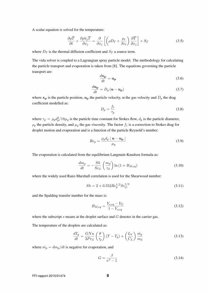
A scalar equation is solved for the temperature:

∂ρT

∂t+∂ρujT

∂xj=

∂

∂xj

[(ρDT +

µtSct

)∂T

∂xj

]+ ST (3.5)

where DT is the thermal diffusion coefficient and ST a source term.

The vida solver is coupled to a Lagrangian spray particle model. The methodology for calculatingthe particle transport and evaporation is taken from [8]. The equations governing the particletransport are:

dxp

dt= up (3.6)

dup

dt= Dp (u− up) (3.7)

where xp is the particle position, up the particle velocity, u the gas velocity and Dp the dragcoefficient modelled as:

Dp =f1τp

(3.8)

where τp = ρpd2p/18µg is the particle time constant for Stokes flow, dp is the particle diameter,

ρp the particle density, and µg the gas viscosity. The factor f1 is a correction to Stokes drag fordroplet motion and evaporation and is a function of the particle Reynold’s number:

Rep =ρgdp | u− up |

µg(3.9)

The evaporation is calculated from the equilibrium Langmuir-Knudsen formula as:

dmp

dt= − Sh

ScG

(md

τd

)ln (1 +BM,eq) (3.10)

where the widely used Ranz-Marshall correlation is used for the Shearwood number:

Sh = 2 + 0.552Re1/2p Sc1/3G (3.11)

and the Spalding transfer number for the mass is:

BM,eq =Ys,eq − YG1− Ys,eq

(3.12)

where the subscript s means at the droplet surface and G denotes in the carrier gas.

The temperature of the droplets are calculated as:

dTpdt

=GNu

3PrG

(θ

τp

)(T − Tp) +

(LVCL

)mp

md(3.13)

where mp = dmp/dt is negative for evaporation, and

G =β

eβ − 1(3.14)


where the non-dimensional evaporation parameter β is:

β = −(3PrGτd

2

)mp

mp(3.15)

PrG = µGCp,G/λG is the gas phase Prandtl number given by the gas phase viscosity (µG), heatcapacity at constant pressure (Cp,G) and thermal conductivity (λG). Nu is the Nusselt number,which is given by the Ranz-Marshall correlation:

Nu = 2 + 0.552Re1/2p Pr1/3G (3.16)

θ = Cp,G/CL is the ratio of of gas heat capacity to liquid heat capacity, TG is the gas temperature,and LV the latent heat of vaporisation.

Droplets break up when the cross flow Weber number exceeds six. The Weber number is given by:

We =ρG(u− up)2rp

σ(3.17)

where rp is the droplet radius and σ is the surface tension.

The evaporated mass is given as a source for the gas phase (equation 3.1 and 3.4), and the changeof particle momentum is given as source for the gas momentum equation (equation 3.2).

The effect on the air temperature due to evaporation is neglected in this simulation, the sourceterm in equation 3.5 is zero. In reality heat is taken from the surrounding air for evaporation of thedroplets and consequently the temperature of air would decrease. This would then create a denserair-chlorine vapour mixture than that calculated as described above. However, in the temperaturesmeasured in the depression during the experiments were not particularly low (down to -10◦C[2]). In this case, for a vapour mass fraction of 50% chlorine vapour, the difference in density ascalculated above compared to the real case is below 10%.

3.2 ARGOS

The Accident Reporting and Guiding Operational System (ARGOS) [9] is a decision supportsystem for enhancing crisis management for incidents involving CBRN releases developedby Beredskapsstyrelsen (Danish Emergency Management Agency, DEMA), Risø NationalLaboratory and PDC-ARGOS in Denmark. Originally developed for supporting decisions fornuclear emergencies, a chemical module has later been included.

For the Jack Rabbit chlorine gas release simulations, the HeavyPuff module in ARGOS was used.This is a box model that was developed by the Technical University of Denmark (DTU, Risø)some years ago, but has never been developed further from the original prototype level [10]. It isdesigned to simulate the behaviour of a heavy gas plume near (up to 500 m) from the source.

In HeavyPuff, the dense gas cloud from an instantaneous release is approximated by a cylinderwith a given radius and height. In the classic box model all properties (concentration, density,absolute temperature, enthalpy difference, et cetera) are assumed to be uniformly distributed


within this volume. The radius grows with a front velocity and the centre of mass moves with theadvection velocity. The vertical mixing of the gas cloud is modelled by an entrainment velocitythrough the top cloud interface, and the enhanced mixing at the front is modelled by the frontentrainment velocity [10].

After the near source region of the dense gas, further dispersion of the gas is simulated by theRimpuff model [9], which is a Gaussian puff model in which the gas cloud is simulated as a seriesof puffs with maximum concentrations in the centre and Gaussian concentration profiles.

3.3 SLAB

The SLAB model [11] is an atmospheric dispersion model for denser-than-air releases, developedin 1990 by Donald L. Ermak of the Lawrence Livermore National Laboratory, Livermore, CA,with support from the U.S. Department of Energy (DOE), USAF Engineering and Services Center,and the American Petroleum Institute. The SLAB model treats denser-than-air releases by solvingone-dimensional spatially averaged equations of momentum, conservation of mass, species, andenergy, and the equation of state (ideal gas). The gas cloud can be treated as a steady plume, puffor a combination of the two depending in the source characteristics. SLAB handles several releasescenarios including ground level and elevated jets, liquid pool evaporation, and instantaneousvolume sources. SLAB is one of the most widely used dense gas models and it is also recognisedas the easiest-to-use dense gas model in the public domain.

SLAB itself is a freeware and in the present investigation the SLAB View Windows graphical userinterface from Lakes Environmental Software was used.

4 Numerical approach

One of the chlorine release trials, test number 5, is used in this case. For this test, two U.S. tonsof chlorine was released. The ambient wind speed was about 1.5 m/s for this case, and the airtemperature at the time of the release was 3.5◦C. For more details concerning this test and theweather conditions see [2].

4.1 Large Eddy Simulation

4.1.1 Computational mesh

The computational domain includes the tank and the depression as specified according to theexperimental setup, see [1] and [2]. The total computational domain consists of a box with alength of 400 meter, a width of 200 meter, and a height of 100 meter. The velocity inlet planeis positioned 100 meter upwind of the tank. Figure 4.1 shows a close-up of the tank and thedepression.

A mesh with about 25 million tetrahedra cells was created. The cells nearest the ground have a


Figure 4.1 The geometrical model of the tank (green) and the depression, which has a flat areawith a diameter of about 24 meters (red) and a 2 meter high hill toward the rim (blue).The total diameter of the depression is 50 meters.

resolution of 20 cm, while the cells grow larger in the vertical direction. The finest resolution is inthe region between the tank and the bottom of the depression with cell lengths of about 2.5 cm.

4.1.2 Boundary conditions

In the experiments, the released material was transported through a 30 cm long pipe beforeentering the environment where subsequent flashing1 of the liquid occurred (some flashing of theliquid also occurred within the pipe). To simulate this would require a separate simulation, as acombination of the resolution required to resolve the processes in the pipe and the subsequentflashing with the large scale simulation of the dispersion of liquid would result in a very timeconsuming simulation. Instead it was planned to start the simulation after the adiabatic expansionof the jet. From thermodynamics, about 12% of the liquid is expected to flash immediately, andbefore air entrainment the jet would then have a diameter of about 0.5 meter.

However, the current code for coupling the variable density solver with Lagrangian spray particlescannot account for such large fractions of liquid because is does not include the volumetricdisplacement of the gas by the droplets. It is valid only for a dilute regime. Therefore a jetconsisting of 10% liquid droplets and 90% vapour was used in the simulation. The area of the jetwas increased to a radius of 0.665 meter.

The vapour is released from a circular area with the dimension specified above. The jet velocitywas chosen to give the release time observed in the experiment (about one minute). The dropletsare released from a number of rings co-located with this area, and the droplets are given radii in

1Flashing means immediate evaporation of liquid due to the pressure difference between storage pressure and theambient pressure.


Height above ground (m) Wind speed (m/s)

2 1.444 1.638 1.8716 1.9032 1.96

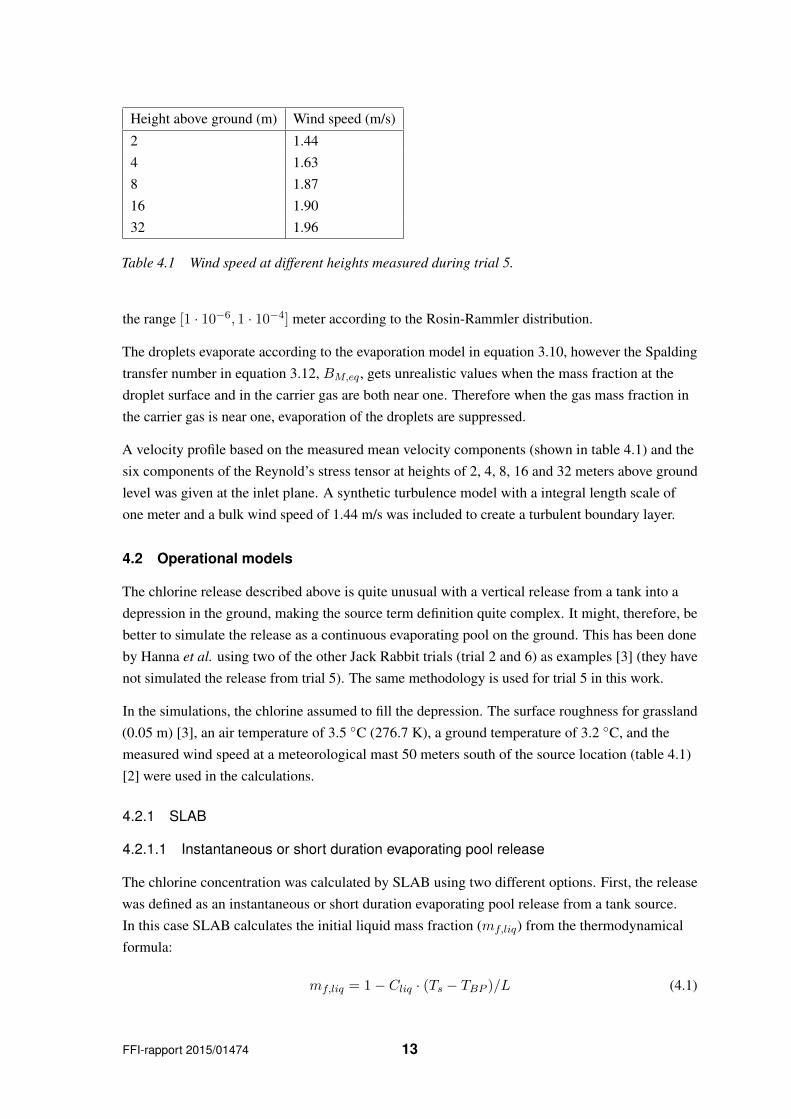
Table 4.1 Wind speed at different heights measured during trial 5.

the range [1 · 10−6, 1 · 10−4] meter according to the Rosin-Rammler distribution.

The droplets evaporate according to the evaporation model in equation 3.10, however the Spaldingtransfer number in equation 3.12, BM,eq, gets unrealistic values when the mass fraction at thedroplet surface and in the carrier gas are both near one. Therefore when the gas mass fraction inthe carrier gas is near one, evaporation of the droplets are suppressed.

A velocity profile based on the measured mean velocity components (shown in table 4.1) and thesix components of the Reynold’s stress tensor at heights of 2, 4, 8, 16 and 32 meters above groundlevel was given at the inlet plane. A synthetic turbulence model with a integral length scale ofone meter and a bulk wind speed of 1.44 m/s was included to create a turbulent boundary layer.

4.2 Operational models

The chlorine release described above is quite unusual with a vertical release from a tank into adepression in the ground, making the source term definition quite complex. It might, therefore, bebetter to simulate the release as a continuous evaporating pool on the ground. This has been doneby Hanna et al. using two of the other Jack Rabbit trials (trial 2 and 6) as examples [3] (they havenot simulated the release from trial 5). The same methodology is used for trial 5 in this work.

In the simulations, the chlorine assumed to fill the depression. The surface roughness for grassland(0.05 m) [3], an air temperature of 3.5 ◦C (276.7 K), a ground temperature of 3.2 ◦C, and themeasured wind speed at a meteorological mast 50 meters south of the source location (table 4.1)[2] were used in the calculations.

4.2.1 SLAB

4.2.1.1 Instantaneous or short duration evaporating pool release

The chlorine concentration was calculated by SLAB using two different options. First, the releasewas defined as an instantaneous or short duration evaporating pool release from a tank source.In this case SLAB calculates the initial liquid mass fraction (mf,liq) from the thermodynamicalformula:

mf,liq = 1− Cliq · (Ts − TBP )/L (4.1)


where Cliq is the liquid heat capacity, Ts the material storage temperature, TBP the materialboiling point and L the heat of vaporisation at the boiling point. Using this formula, a liquidmass fraction of 0.878 is calculated. The release is then calculated from a combination of twosources: an instantaneous volume source (mass fraction 0.122), which could be either pure vapouror a mixture of vapour and liquid droplets, and a short-duration ground level area source (massfraction 0.878). The source area was taken as the area of the 50 m diameter depression (1960 m2)and the total mass released was 1826 kg. The temperature of the source material was set to theboiling temperature of chlorine, 239.1 K.

4.2.1.2 As an evaporation pool

In addition, the chlorine concentration from an evaporating pool from the same source area as usedabove (1960 m2), but without any instantaneous vapour or liquid droplet fraction, was calculated.Also for this case, the temperature of the source material was set to 239.1 K.

The source duration had to be estimated from the videos recorded during the field trials or calcu-lated. In the release, quite a lot of the released material is transported out of the depression duringthe release. However once the release is finished, the gas fills out the depression and remains inthe depression for at least five minutes (which is the duration of the available videos) and is veryslowly transported out. Briggs et al. developed a model for dense gas removal from a valley bycross-winds [4], also used in [3]. Even though this is a model for the removal of dense gas trappedin a valley, it has been used to set the evaporation rate from a pool filling out the depression inthe current simulation. The model gives a source duration of 900 seconds for a wind speed of1.44 m/s (although this might be too high wind speed for this model, the velocity closer to theevaporating surface would be more appropriate; this would give an even longer evaporation time).It was therefore decided to use four different pool durations: 60, 120, 180 and 900 seconds. Therelease rate (source rate) was adjusted accordingly (30.4 kg/s, 15.2 kg/s, 10.1 kg/s and 2.0 kg/s) inorder to obtain the total source mass (1826 kg).

4.2.2 ARGOS

The chlorine concentration was calculated by ARGOS as a release from a pool with diameter50 meter in the same way as described for SLAB in chapter 4.2.1.2 (no initial vapour fraction).The chlorine was released with two different release rates: 30.4 kg/s over 60 seconds and 15.2 kg/sover 120 seconds. The surface under the pool and the surrounding environment were set to drysand.


Height (meter) Maximum concentration (mg/m3)

0.5 1.4·105

1.0 2.0·104

1.5 9.9·103

2.0 9.9·103

Table 5.1 Maximum chlorine vapour concentration 25 meters downwind at different heights.

5 Results

5.1 Dispersion

5.1.1 LES

Figure 5.1 shows the concentration of chlorine vapour in a vertical plane through the sourcelocation at various time steps. Figure 5.2 shows the simulated three dimensional vapour cloud attwo time steps.

During the release, at first the gas is transported symmetrically outwards in all directions closeto the ground. The transport along the ground is opposed by the incoming ambient velocity fieldupwind, gravitational forces at the rise toward the rim of the depression, and by frictional forces,and the gas soon falls back into the depression. Initially a lot of mixing in the vertical directionoccurs. Toward the end of the release however, the vertical mixing diminish, and after the releasehas finished, the gas remains quite still in the depression for a long time, and is slowly transportedout of the depression. This is very similar to what was observed in the experiments.

Figure 5.3 shows the predicted vapour concentrations 25 and 50 meters downwind the releasepoint as function of time. This is five seconds averages of the maximum concentrations. However,the concentration drops rapidly with height in the simulation. Table 5.1 gives the predictedmaximum concentration at height of 0.5, 1, 1.5 and 2 meters above ground 25 meters downwind.The maximum concentration shown in figure 5.3 is taken fairly close to the ground.

Figure 5.4 shows the concentration profiles measured with the Jaz UV-Viz sensors during theexperiment. The concentration peaks corresponds fairly well with the maximum concentrationmeasured in the experiment, see also figure 5.6. However, the measured time concentrationprofiles decrease much quicker than the simulated time concentration profiles. It should be notedthat the maximum concentration is not necessarily found directly downwind; kinematic blockingof the gas upwind and the gravitational forces blocking the dispersion at the edges may inducebuild up of vapour at these locations.

Figure 5.5 shows the predicted amount of vapour inside the depression as function of time.If this curve is extrapolated, it would take a long time before all the gas is transported out ofthe depression (about one hour). This is a much longer time than what was observed in theexperiments. Both the transport of vapour out of the depression and the vertical mixing of the


(a) 10 s

(b) 30 s

(c) 50 s

(d) 90 s

Figure 5.1 The chlorine vapour concentration in a vertical plane through the source at varioustime steps after the start of the release. The release starts at t = 0 s and ends att = 60 s. The mean wind direction is in the positive x-direction.


(a) 30 s

(b) 60 s

Figure 5.2 The simulated vapour cloud at various time steps after the start of the release. Therelease starts at t = 0 s and ends at t = 60 s.


(a) 25 meter

(b) 50 meter

Figure 5.3 The predicted concentration 25 and 50 meters downwind the release point. Thestapled line denotes the end of the release.


(a) 25 meter

(b) 50 meter

Figure 5.4 The chlorine vapour concentration 25 and 50 meters downwind the release pointmeasured with the Jaz UV-Viz sensors. The sensor at 25 meters is almost directlydownwind of the source (within 20◦), while the sensor at 50 meters is almost 90◦ off.


Figure 5.5 The predicted chlorine capour mass contained in the depression as function of time.

vapour downwind the depression is underestimated. As long as the release occurs, the motion ofthe dense gas jet induces all the motion near the source location, and the simulation shows goodagreement with the experiment (even though the characteristics of the jet is different from theexperimental jet). After the release has finished however, some discrepancies becomes apparent.The reason for this is most likely that the atmospheric boundary layer near the ground is too poorlyresolved in the simulation.


In figure 5.6 a plot of the centreline chlorine concentration at different distances from the sourceis shown. In addition, the maximum obtained readings from field measurements at three distances(25 , 50 and 100 meters) and the maximum concentration levels with LES at two distances(25, and 50 meters) from the source are also shown.

When evaporation from a pool is selected in SLAB, the maximum airborne concentration isachieved at about 22 m from the source for all three source durations. This corresponds with theedge of the 50 m diameter depression. The chlorine cloud gets more and more diluted as it travelsfurther away from the source.

Figure 5.6 shows that SLAB predicts a higher initial chlorine concentration with the instantaneousor short duration pool simulation compared to evaporation from a pool. This is because a part of


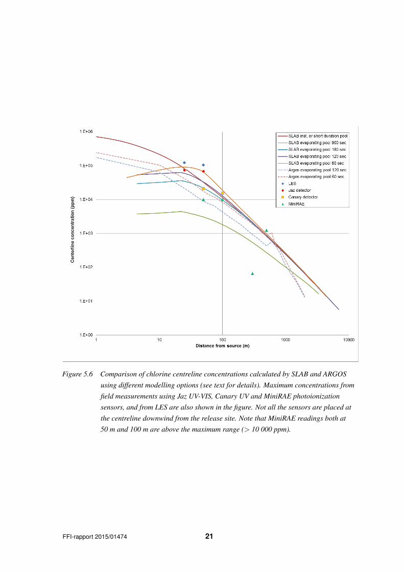
Figure 5.6 Comparison of chlorine centreline concentrations calculated by SLAB and ARGOSusing different modelling options (see text for details). Maximum concentrations fromfield measurements using Jaz UV-VIS, Canary UV and MiniRAE photoionizationsensors, and from LES are also shown in the figure. Not all the sensors are placed atthe centreline downwind from the release site. Note that MiniRAE readings both at50 m and 100 m are above the maximum range (> 10 000 ppm).


the release (12.8 %) during the first method was calculated as either pure vapour or a mixture ofvapour and airborne liquid droplets, which, since SLAB does not take topography into account, isquickly transported downwind. In our view it is more realistic to represent the chlorine containedin the depression as a liquid pool only (no initial vapour or airborne droplet phase). The fourSLAB calculations with evaporating pool only gave different air concentrations close to the source,but approximately the same concentration of chlorine farther downwind, i.e. more than about300 meter downwind from the source, except for the longest pool duration (900 seconds).

Heavy gas calculations using ARGOS was carried out using the pool only method described forSLAB above. The calculated chlorine concentration outside the depression (more than 25 m) ishigher with SLAB (up to about a factor four) compared to the concentration calculated by ARGOSusing the same pool duration. The difference between SLAB and ARGOS gets smaller when thecloud moves towards 500 m from the source.

At 500 m distance, Gaussian puff calculation takes over form the box model. The discontinuityin the ARGOS results is due to the change of dispersion models at this distance. The calculatedconcentration drops quicker with distance after this transition. This is reasonable as the chlorinecloud does not behave like a dense cloud anymore and therefore dilutes more quickly in thesurrounding air

There are too few concentration measurements from vapour detectors in the area to be able todraw any conclusions on which method that best predicts the concentration. The measurementsfits relatively well with all the performed simulations, except for the SLAB simulation with900 seconds pool duration. This indicates that the duration calculated with the model by Briggset al is too long for this modelling procedure, even though this corresponds better with theobservations from the experiment.

The plume widths at 50 m and 500 m from the source centre are shown in table 5.2. The differencebetween the plume widths for AEGL-1, AEGL-2 and AEGL-3 levels are very small, and thereforethe plume widths for only one concentration limit are shown. The initial plume width (at 50 meter)is larger for the instantaneous or short duration evaporating pool release with SLAB and smallerwith ARGOS compared to the release from a pool using SLAB. At 50 meter distance, the plumewidth is larger from 120 second pool duration compared to shorter and longer pool durations. At500 meter from the source centre, all four SLAB calculations gave almost the same plume width,except from the longest pool duration, whereas ARGOS gave a wider plume.

With LES, the width of the plume to the AEGL concentration levels 50 meters downwind of therelease is about 50 meters at the end of the release, and grows to about 150 meters after the releasestops.

The dimensions of the gas cloud was estimated by cameras. It is not clear to the authors at whatconcentration level the gas was detected. From these cameras a cloud with of about 300 meters isestimated three minutes after start of the release. The center of the plume is by that time about 160meters from the release location. It should however be noted that because the wind direction shifts,


Model Pool duration (sec) Distance from source centre50 m 500 m

SLAB-inst 260 500SLAB-pool 60 180 470SLAB-pool 120 240 500SLAB-pool 180 190 480SLAB-pool 900 110 300ARGOS-pool 60 120 600ARGOS-pool 120 110 600

Table 5.2 Maximum plume width (m) at 50 m and 500 m from source centre. SLAB-inst iscalculated as an instantaneous or short duration evaporating pool release whileSLAB-pool and ARGOS-pool is calculated as an evaporating pool with different poolduration times.

the plume has travelled a longer distance than that at this point. The width then decrease with timeto 200 - 250 meters.

5.3 The wind field

Figure 5.7 shows velocity profile given as input to the simulation together with the profile from thesimulation at a vertical line 50 meters downwind the inlet plane (and 25 meters upwind the nearestrim of the depression). The velocity profile from the simulation is an average of 600 time stepsbefore the release is started. The measured velocity profile is fairly well reproduced.

Figure 5.8 shows the streamwise velocity before and during the release. The mean velocity plotsshow time averages over 470 seconds before the release, and for the duration of the release (60seconds) for the release. It is evident that the dense gas release reduce the velocity near the release,while the fluctuations are increased.

Figure 5.9 shows the difference between the mean streamwise velocity before the release and themean during the release as function of time at four locations, two within the depression and twolocations downwind. The mean before the release is time averaged over 470 seconds, while themean velocity during the release is the mean velocity over the given time since the start of therelease. The velocities are shown in heights of one and two meters above ground. The difference iscalculated as:

Udiff =U(t)− U(t = 0)

U(t = 0)(5.1)

Figure 5.10 shows the corresponding velocity difference for the vertical component. At theheight of one meter, the streamwise velocities at the two locations within the depression firsthave a brief rise, then quickly drops, especially at the downwind location. Also at the rim of thedepression there is a decrease in velocity at one meter, while the velocity at the location downwindthe depression is not so affected by the dense gas. At two meters, the upwind location inside


Figure 5.7 The streamwise velocity profiles measured in the experiment (and given as inletconditions to the LES), and from the simulation 50 meters downwind the inlet plane.


(a) U before release (b) U during release

(c) U before release (d) U during release

(e) URMS before release (f) URMS during release

Figure 5.8 The instantaneous streamwise velocity (U ), the mean streamwise velocity (U ), and theroot-mean-square (URMS) before the release (a, c, e) and during the release (b, d, f).U and U are shown i the range < −2 (blue) , 2 (red) > m/s, with green being lowvelocities, URMS are shown in the range < 0 (blue) , 1 (red) > m/s.


(a) Height = 1 meter

(b) Height = 2 meter

Figure 5.9 The difference of the mean streamwise velocity before and during the release asfunction of time. The release starts at t = 0 and ends at t = 120 s. The locations atx = −10 and x = 10 are within the depression (10 meters upwind and downwind ofthe tank respectively), while x = 25 are at the edge of the depression and x = 50

downwind. The velocity at t = 0 is the time average up to the point where the releasestarts, while the other times are time averages for the period since the start of therelease.


(a) Height = 1 meter

(b) Height = 2 meter

Figure 5.10 The difference of the mean vertical velocity before and during the release as functionof time. The release starts at t = 0 and ends at t = 120 s. The locations at x = −10and x = 10 are within the depression (10 meters upwind and downwind of the tankrespectively), while x = 25 are at the edge of the depression and x = 50 downwind.The velocity at t = 0 is the time average up to the point where the release starts,while the other times are time averages for the period since the start of the release.


the depression also shows a decrease in the velocities, while the other locations are relativelyunaffected, or shows a slight increase in the velocity.

For the vertical velocity component, at first there are a lot of movement within the depression;fairly large vortices will be induced by the release jet. However, these structures diminish aftersome time, and the vertical velocity is subdued as compared to the situation before the release.

6 Concluding remarks

6.1 Large eddy simulations

The condition of the release jet was not measured very precisely during the experiments, sothe quantity of vapour and liquid must be estimated based on analytical models. From purethermodynamics, about 12% is expected to flash immediately due to the difference between thestorage pressure and the ambient pressure. Thus most of the material is expected to be releasedas liquid. Some of this liquid will be dispersed as airborne droplets (which evaporates over time),some will evaporate immediately and some liquid will form a pool on the ground and subsequentlyevaporate, creating a secondary vapour source.

In the current CFD modelling approach it is not possible to take into account such a large quantityof liquid compared to vapour. Instead only 10% was released as liquid droplets and the rest re-leased as vapour. There is therefore a discrepancy between the actual release jet and the simulatedjet, and this will likely result in some differences in the velocity fields and the corresponding gasdispersion.

Another deficiency with the current LES methodology is the treatment of temperature. The energyequation is not solved explicitly, instead a scalar transport equation for temperature is solved.The gas temperature calculated by this is used for the Lagrangian spray model for calculatingthe evaporation and the temperature of the droplets, but there is no coupling back to the gastemperature transport equation. This will lead to an overestimation of the gas temperature, andthereby an underestimation of the density.

Even so, within the depression, where the dynamics are to a large extent driven by the momentumof the release jet, there is a fairly good agreement between the experiment and the simulation,indicating that the dynamics are quite well captured.

Outside of the depression there seems to be an underestimation of the mixing of the gas in thesimulation when compared to the experiment. One reason for this is probably that the resolution ofthe computational mesh is too coarse to resolve the atmospheric boundary layer in this region.


An approach described by Hanna et al. in which evaporation from a pool with the dimensionsof the depression, where the evaporation rate is specified according to a model of dense gas


removal from a valley by cross-wind, has been tested both with SLAB and ARGOS. For bothmodels good agreement with the experimental results can be found, however it is quite dependenton the evaporation rate and it is not obvious how to specify this rate a priori. In fact, the ratecorresponding to the vapour removal time frame most consistent with the experimental observation(15 minutes) yields the least agreement with the experimental measurements of downwindconcentration of vapour.

The dense gas atmospheric dispersion model SLAB predicts a higher initial chlorine concentrationusing the instantaneous or short duration pool option, compared to evaporation from a pool only.It is believed that the pool only option better represent the release from the depression used in theJack Rabbit exercise because the gas is trapped inside the depression for a longer time compared toa release in a flat area.

Heavy gas calculations using ARGOS was carried out as a release from a pool only in the sameway as described for SLAB. The predicted chlorine concentration outside the depression islower (about 1

4 ) than calculated by SLAB for the same pool duration times. This could partly beexplained by the somewhat wider plume predicted by ARGOS compared to SLAB, especially atlonger distances from the source.

6.3 Further work

The Jack Rabbit field trials was designed to use a relatively small scale release (two tons) tosimulate a much larger release (twenty tons). However, it is observed that the source behaviouris non-linear with increasing release volumes [12]. Therefore the test program continues as JackRabbit II, in which experiments with the release of 5-20 tons of chlorine will be conducted. Forthe field trials in 2015 a mock urban test environment was constructed for the trials, while theexperiments in 2016 will be in open terrain. This time there will be measurements of chlorinevapour concentrations up to 11 km downwind the release site, as well as within the mock urban en-vironment. FFI has contributed with numerical simulations in order to assist with the experimentalsetup and sensor placement. FFI was also present at the 2015 trials, and we will have access to allthe experimental data from these field trials.

We are quite confident that the LES methodology used for the Jack Rabbit simulations cancapture the dynamics of the releases at least in the near field. Data from Jack Rabbit II as well asnumerical simulations will be used to investigate dense gas releases further and in more detail.Jack Rabbit II will also be more appropriate for testing the faster hazard prediction tools, as it isfor dispersion over large areas that these models really have their use.


References

[1] Donald P. Storwold JR. Detailed test plan for the jack rabbit test program. Technical report,West Desert Test Center, U.S. Army Dugway Proving Ground, March 2010. ATEC ProjectNo. 2012-DT-DPG-SNIMT-E5835, WDTC Document No. WDTC-TP-10-011.

[2] Thomas Vik. Jack rabbit field trials - systematisering av eksperimentelle resultater. FFI-rapport2013/02771, Forsvarets forskningsinstitutt, 2013. In norwegian.

[3] Steven Hanna, Rex Britter, Edward Argenta, and Joseph Chang. The jack rabbit chlorinerelease experiments: Implications of dense gas removal from a depression and downwindconcentrations. Journal of hazardous materials, 213:406–412, 2012.

[4] Gary A Briggs, Roger S Thompson, and William H Snyder. Dense gas removal from a valleyby crosswinds. Journal of Hazardous Materials, 24(1):1–38, 1990.

[5] Timothy J Bauer. Comparison of chlorine and ammonia concentration field trial data withcalculated results from a gaussian atmospheric transport and dispersion model. Journal ofhazardous materials, 254:325–335, 2013.

[6] John D Hearn, Richard Weber, Robert Nichols, Michael V Henley, and Shannon Fox.Deposition of cl 2 on soils during outdoor releases. Journal of hazardous materials, 252:107–114, 2013.

[7] http://www.cascadetechnologies.com/.

[8] RS Miller, K Harstad, and J Bellan. Evaluation of equilibrium and non-equilibrium evapora-tion models for many-droplet gas-liquid flow simulations. International Journal of MultiphaseFlow, 24(6):1025–1055, 1998.

[9] Danish Emergency Management Agency, Risø DTU National Laboratory, Danish Meteorolo-gical Institute, and Prolog Development Center AS. Whitepaper, ARGOS CBRN InformationSystem for Emergency Management, March 2011.

[10] Morten Nielsen. Dense gas dispersion in the atmosphere. Technical report, Risø NationalLaboratory, Roskilde, Denmark, September 1998. Risø-R-1030 (EN).

[11] Donald R Ermak. User’s manul for SLAB: an atmospheric dispersion model for denser-than-air releases, June 1990. UCRL-MA-105607.

[12] Shannon Fox. The Jack Rabbit II Program. Presentation at the Jack Rabbit II StakeholderKickoff Meeting, American Chemistry Council HQ, Washington D.C., March 27, 2015.


thomas vik, john aa tørnes and bjørn anders p. reif · ffi-rapport 2015/01474 simulations of the...

Documents