this study was funded and prepared for the u.s. army corps ... · u.s. geological survey ... wind...

Suggested citation:

Rohweder, J., Rogala, J. T., Johnson, B. L., Anderson, D., Clark, S., Chamberlin, F., Potter, D.,

and Runyon, K., 2012, Application of Wind Fetch and Wave Models for Habitat Rehabilitation

and Enhancement Projects – 2012 Update. Contract report prepared for U.S. Army Corps of

Engineers’ Upper Mississippi River Restoration – Environmental Management Program. 52 p.

This study was funded and prepared for the U.S. Army Corps of Engineers’ Upper Mississippi

River Restoration - Environmental Management Program

Application of Wind Fetch and Wave Models for Habitat Rehabilitation and Enhancement Projects – 2012 Update

By

Jason Rohweder

James Rogala

Barry Johnson

U.S. Geological Survey

Upper Midwest Environmental Sciences Center

2630 Fanta Reed Road

La Crosse, Wisconsin 54603

And

Dennis Anderson

Steve Clark

Ferris Chamberlin

David Potter

U.S. Army Corps of Engineers

St. Paul District

190 5th Street East, Suite 401

St. Paul, Minnesota 55101-1638

And

Kip Runyon

U.S. Army Corps of Engineers

St. Louis District

1222 Spruce Street

St. Louis, Missouri 63103-2833

December 2012 [Revised 07/08/14]

Mention of trade names or commercial products does not constitute endorsement or

recommendation for use by the U.S. Department of Interior, U.S. Geological Survey or the U.S.

Army Corps of Engineers.

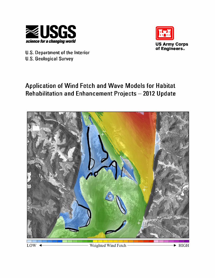
Cover image is a depiction of management scenario 4, weighted wind fetch results for the

Harper’s Slough Habitat Rehabilitation and Enhancement Project in Navigation Pool 9, Upper

Mississippi River System. The background image is a grayscale version of a 2009 National

Agriculture Imagery Program aerial photograph.

i

ABSTRACT .................................................................................................................................................................................... 1

KEY WORDS ................................................................................................................................................................................. 1

INTRODUCTION .......................................................................................................................................................................... 1

TOOLBOX INSTALLATION ....................................................................................................................................................... 2

WIND FETCH MODEL ................................................................................................................................................................ 5

INTRODUCTION ............................................................................................................................................................................. 5 METHODOLOGY ............................................................................................................................................................................ 5 WIND FETCH MODEL VALIDATION .............................................................................................................................................. 11

Two-sample permutation test for locations .......................................................................................................................... 13

WAVE MODEL ............................................................................................................................................................................ 14

INTRODUCTION ........................................................................................................................................................................... 14 ASSUMPTIONS AND MODEL LIMITATIONS .................................................................................................................................... 17 METHODOLOGY .......................................................................................................................................................................... 18

Adjusting Wind Speed Data .................................................................................................................................................. 19 Deep Water Test ................................................................................................................................................................... 20 Significant Wave Height ....................................................................................................................................................... 23 Wave Length ......................................................................................................................................................................... 24 Spectral Peak Wave Period .................................................................................................................................................. 25 Maximum Orbital Wave Velocity ......................................................................................................................................... 25 Shear Stress .......................................................................................................................................................................... 25

DELINEATE AREA OF POTENTIAL EFFECTS MODEL ................................................................................................... 27

ST. PAUL DISTRICT ANALYSES ............................................................................................................................................ 29

STUDY AREAS ............................................................................................................................................................................ 29 Harper’s Slough HREP ........................................................................................................................................................ 30

WEIGHTED WIND FETCH ANALYSIS ............................................................................................................................................ 32 Land Raster Input Data ........................................................................................................................................................ 32 Wind Direction Input Data ................................................................................................................................................... 33 Weighted Wind Fetch ........................................................................................................................................................... 34 Analysis Results .................................................................................................................................................................... 35 Discussion ............................................................................................................................................................................ 40

SEDIMENT SUSPENSION PROBABILITY ANALYSIS ......................................................................................................................... 40 Analysis Results .................................................................................................................................................................... 41 Discussion ............................................................................................................................................................................ 46

SPATIAL DATASETS USED IN ANALYSES .......................................................................................................................... 46

UMRR-EMP LTRMP 2010 LAND COVER/LAND USE DATA FOR THE UPPER MISSISSIPPI RIVER SYSTEM ................................... 46 Originator ............................................................................................................................................................................ 46 Abstract ................................................................................................................................................................................ 46

UMRR-EMP LTRMP BATHYMETRIC DATA FOR THE UPPER MISSISSIPPI AND ILLINOIS RIVERS ................................................. 47 Originator ............................................................................................................................................................................ 47 Abstract ................................................................................................................................................................................ 47 Online Linkage ..................................................................................................................................................................... 47

ACKNOWLEDGEMENTS ......................................................................................................................................................... 47

REFERENCES CITED ................................................................................................................................................................ 47

TABLE 1. TABULAR SUMMARIZATION OF WIND FETCH MEASUREMENTS CALCULATED USING THE TWO DIFFERENT

METHODS ............................................................................................................................................................ 13 TABLE 2. SUMMARIZATION OF RESULTS USED TO TEST FOR DEEP VS. SHALLOW WATER .............................................. 23

ii

FIGURE 1. WINDOWS EXPLORER VIEW OF EXTRACTED FILES ......................................................................................... 3 FIGURE 2. ARCTOOLBOX VIEW OF WAVE TOOLS ............................................................................................................ 4 FIGURE 3. WINDOWS DIALOG FOR SELECTING WAVES2012 TOOLBOX .......................................................................... 5 FIGURE 4. SAMPLE TEXT FILE WITH FETCH DIRECTION AND DIRECTION WEIGHTING INPUT DATA .................................. 6 FIGURE 5. FETCH MODEL DIALOG WINDOW PROMPTING USER INPUT ............................................................................. 7 FIGURE 6. EXAMPLE DEPICTIONS OF WIND FETCH CALCULATED USING THE DIFFERENT METHODS ................................ 8 FIGURE 7. SAMPLE WIND FETCH MODEL RESULTS FOR SWAN LAKE HABITAT REHABILITATION AND ENCHANTMENT

PROJECT .............................................................................................................................................................. 10 FIGURE 8. WIND FETCH CELL LOCATIONS AND PREVAILING WIND DIRECTIONS USED FOR MODEL VALIDATION ........... 12 FIGURE 9. RESULTS FOR TWO-SAMPLE PERMUTATION TEST FOR LOCATIONS .............................................................. 14 FIGURE 10. WAVE MODEL DIALOG WINDOW PROMPTING USER INPUT ......................................................................... 15 FIGURE 11. SAMPLE TEXT FILE DEPICTING VALID INPUT VALUES FOR WIND DATA IN WAVE MODEL ............................ 16 FIGURE 12. VISUAL DEPICTION OF USACE SUBAREAS USED TO CALCULATE AVERAGE WATER DEPTH ....................... 22 FIGURE 13. SAMPLE WAVE MODEL OUTPUTS FOR SCENARIO 4, CAPOLI SLOUGH HABITAT REHABILITATION AND

ENHANCEMENT PROJECT .................................................................................................................................... 26 FIGURE 14. DIAGRAM DEPICTING RELATIONSHIPS OF INPUT AND OUTPUT PARAMETERS USED WITHIN WAVE MODEL . 27 FIGURE 15. DELINEATE AREA OF POTENTIAL EFFECTS MODEL DIALOG WINDOW ....................................................... 28 FIGURE 16. RESULTS FROM DELINEATE AREA OF POTENTIAL EFFECTS MODEL FOR HARPER’S SLOUGH HREP USING

EXISTING CONDITIONS (2015) AND SCENARIO 4 WEIGHTED WIND FETCH PRODUCTS AS INPUTS .......................... 29 FIGURE 17. LOCATION OF POOL 9 AND HARPER’S SLOUGH HABITAT REHABILITATION AND ENHANCEMENT PROJECT

........................................................................................................................................................................... 30 FIGURE 18. HARPER’S SLOUGH HABITAT REHABILITATION AND ENHANCEMENT PROJECT MAP WITH FEATURE LABELS

........................................................................................................................................................................... 32 FIGURE 19. LOCATION OF REVISED ISLAND ADDITIONS TO HARPER'S SLOUGH HREP AREA ........................................ 33 FIGURE 20. SAMPLE NATIONAL CLIMATIC DATA CENTER, LOCAL CLIMATOLOGICAL DATA SUMMARY SHEET .......... 34 FIGURE 21. BREAKDOWN OF WIND DIRECTIONS COLLECTED FOR LA CROSSE MUNICIPAL AIRPORT SITE .................... 35 FIGURE 22. WEIGHTED WIND FETCH RESULTS FOR THE HARPER’S SLOUGH HABITAT REHABILITATION AND

ENHANCEMENT PROJECT .................................................................................................................................... 36 FIGURE 23. DIFFERENCE IN WEIGHTED WIND FETCH FROM THE NO-ACTION (2065) CONDITIONS MANAGEMENT

SCENARIO TO THE EXISTING CONDITIONS (2015) SCENARIO AND SCENARIOS 1, 2, 3, AND 4 FOR THE HARPER’S

SLOUGH HREP ................................................................................................................................................... 38 FIGURE 24 GRAPH DEPICTING THE PERCENT DECREASE IN WEIGHTED WIND FETCH FROM THE NO-ACTION (2065)

MANAGEMENT SCENARIO TO THE EXISTING CONDITIONS (2015) SCENARIO AND SCENARIOS 1, 2, 3, AND 4 FOR

THE HARPER’S SLOUGH HABITAT REHABILITATION AND ENHANCEMENT PROJECT AREA OF INTEREST ............. 39 FIGURE 25. DIAGRAM EXPLAINING PROCESS FOR CALCULATING PERCENT OF DAYS CAPABLE OF SUSPENDING

SEDIMENTS .......................................................................................................................................................... 41 FIGURE 26. SEDIMENT SUSPENSION PROBABILITY RESULTS FOR THE HARPER’S SLOUGH HREP ................................. 42 FIGURE 27. DIFFERENCE IN SEDIMENT SUSPENSION PROBABILITY FROM THE NO-ACTION (2065) CONDITIONS

MANAGEMENT SCENARIO TO THE EXISTING CONDITIONS (2015) SCENARIO AND SCENARIOS 1, 2, 3, AND 4 FOR

THE HARPER’S SLOUGH HREP ........................................................................................................................... 44 FIGURE 28 GRAPH DEPICTING THE PERCENT DECREASE IN SEDIMENT SUSPENSION PROBABILITY FROM THE NO-ACTION

(2065) MANAGEMENT SCENARIO TO THE EXISTING CONDITIONS (2015) SCENARIO AND SCENARIOS 1, 2, 3, AND 4

FOR THE HARPER’S SLOUGH HABITAT REHABILITATION AND ENHANCEMENT PROJECT .................................... 45

1

Models based upon coastal engineering equations have been developed to quantify wind fetch

length and several physical wave characteristics including significant height, length, peak period,

maximum orbital velocity, and shear stress. These models, developed using Environmental

Systems Research Institute’s ArcGIS 10.x Geographic Information System platform, were used

to quantify differences in proposed island construction designs for the Harper’s Slough Habitat

Rehabilitation and Enhancement Project in the U.S. Army Corps of Engineers St. Paul District.

Weighted wind fetch was calculated using land cover data supplied by the Upper Mississippi

River Restoration – Environmental Management Program’s (UMRR-EMP) Long Term Resource

Monitoring Program (LTRMP) for each island design scenario. Figures and graphs were created

to depict the results of this analysis. The difference in weighted wind fetch from existing

conditions to each potential future island design was calculated. A simplistic method for

calculating sediment suspension probability was also applied. This analysis involved

determining the percentage of days that maximum orbital wave velocity calculated over the

growing seasons of 2008-2012 exceeded a threshold value taken from the literature where fine

unconsolidated sediments may become suspended. This analysis also evaluated the difference in

sediment suspension probability from existing conditions to the potential island designs.

Bathymetric data used in the analysis were collected from the UMRR-EMP LTRMP and wind

direction and magnitude data were collected from the National Oceanic and Atmospheric

Administration, National Climatic Data Center.

Upper Mississippi River Restoration, Environmental Management Program, Long Term

Resource Monitoring Program, Habitat Rehabilitation and Enhancement Project, Wind Fetch,

Sediment Suspension Probability, Significant Wave Height, Wave Length, Spectral Peak Wave

Period, Maximum Orbital Wave Velocity, Shear Stress, Harper’s Slough, Geographic

Information System

The U.S. Army Corps of Engineers (USACE) tasked the Upper Midwest Environmental

Sciences Center (UMESC) of the U.S. Geological Survey (USGS) with upgrading geospatial

models developed to quantify wind fetch length and calculate several physical wave

characteristics that can be altered by Habitat Rehabilitation and Enhancement Projects (HREP).

The models originally developed in ESRI ArcGIS software version 9.3 were upgraded to be able

to operate using the most current version (10.x). Within the wind fetch model a feature was

added to allow the automated calculation of weighted wind fetch results. Features were also

added to the wave model to allow the automated calculation of sediment suspension probability

and also a revised water density parameter which accepts a raster surface as input. A new model

was also developed to allow the user to delineate the area of potential effects based on the

magnitude of difference between alternative project design results.

Using the upgraded models, UMESC was then asked to perform specific analyses to model

weighted wind fetch and also calculate the probability that fine unconsolidated particles would

be suspended due to wind-generated waves for Harper’s Slough HREP within the St. Paul

2

District of the USACE. Wave output data were created with algorithms that used wind fetch,

wind direction, wind speed, and water depth as primary input parameters. The results of these

analyses depict how wind fetch and fine unconsolidated particle suspension are affected by

alternative HREP management scenarios, allowing managers to quantify gains or losses between

these proposed management scenarios.

To use the wind fetch and wave models, there are some preliminary steps that need to be

followed for them to function correctly on the computer. First are a few software requirements

that need to be met:

1. ArcGIS 10.x

2. A Spatial Analyst License

3. Python 2.4 or more recent (Automatically installed with ArcGIS)

4. Pywin32 (Python for Windows extension)

Pywin32 allows Python to communicate with COM servers such as ArcGIS, Microsoft Excel,

Microsoft Word, etc. Python scripting in ArcGIS cannot work without this extension. This

extension can be downloaded at:

http://sourceforge.net/projects/pywin32/files/pywin32/

Once these software requirements are met, the user needs to:

1. Extract the .zip file “Waves2012.zip” to a project directory on your hard drive (Figure 1)

2. Open ArcMap 10.x and activate ArcToolbox if not already activated (Geoprocessing ->

ArcToolbox)

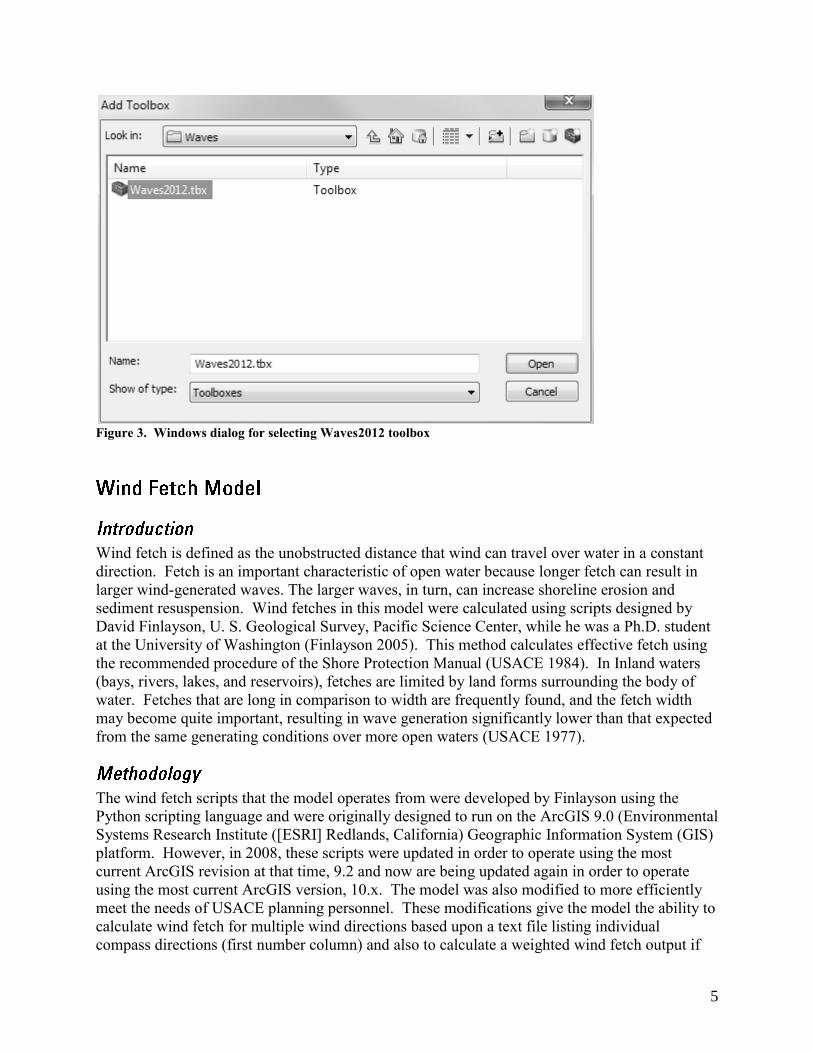
3. Right-click inside the ArcToolbox panel and select Add Toolbox… (Figure 2)

4. Open the extracted folder Waves2012 and click on the Waves2012 toolbox icon.

http://sourceforge.net/projects/pywin32/files/pywin32/

3

Figure 1. Windows Explorer view of extracted files

4

Figure 2. ArcToolbox view of wave tools

You should now be ready to run the wind fetch and wave models within the Waves toolbox

(Figure 3).

5

Figure 3. Windows dialog for selecting Waves2012 toolbox

Wind fetch is defined as the unobstructed distance that wind can travel over water in a constant

direction. Fetch is an important characteristic of open water because longer fetch can result in

larger wind-generated waves. The larger waves, in turn, can increase shoreline erosion and

sediment resuspension. Wind fetches in this model were calculated using scripts designed by

David Finlayson, U. S. Geological Survey, Pacific Science Center, while he was a Ph.D. student

at the University of Washington (Finlayson 2005). This method calculates effective fetch using

the recommended procedure of the Shore Protection Manual (USACE 1984). In Inland waters

(bays, rivers, lakes, and reservoirs), fetches are limited by land forms surrounding the body of

water. Fetches that are long in comparison to width are frequently found, and the fetch width

may become quite important, resulting in wave generation significantly lower than that expected

from the same generating conditions over more open waters (USACE 1977).

The wind fetch scripts that the model operates from were developed by Finlayson using the

Python scripting language and were originally designed to run on the ArcGIS 9.0 (Environmental

Systems Research Institute ([ESRI] Redlands, California) Geographic Information System (GIS)

platform. However, in 2008, these scripts were updated in order to operate using the most

current ArcGIS revision at that time, 9.2 and now are being updated again in order to operate

using the most current ArcGIS version, 10.x. The model was also modified to more efficiently

meet the needs of USACE planning personnel. These modifications give the model the ability to

calculate wind fetch for multiple wind directions based upon a text file listing individual

compass directions (first number column) and also to calculate a weighted wind fetch output if

6

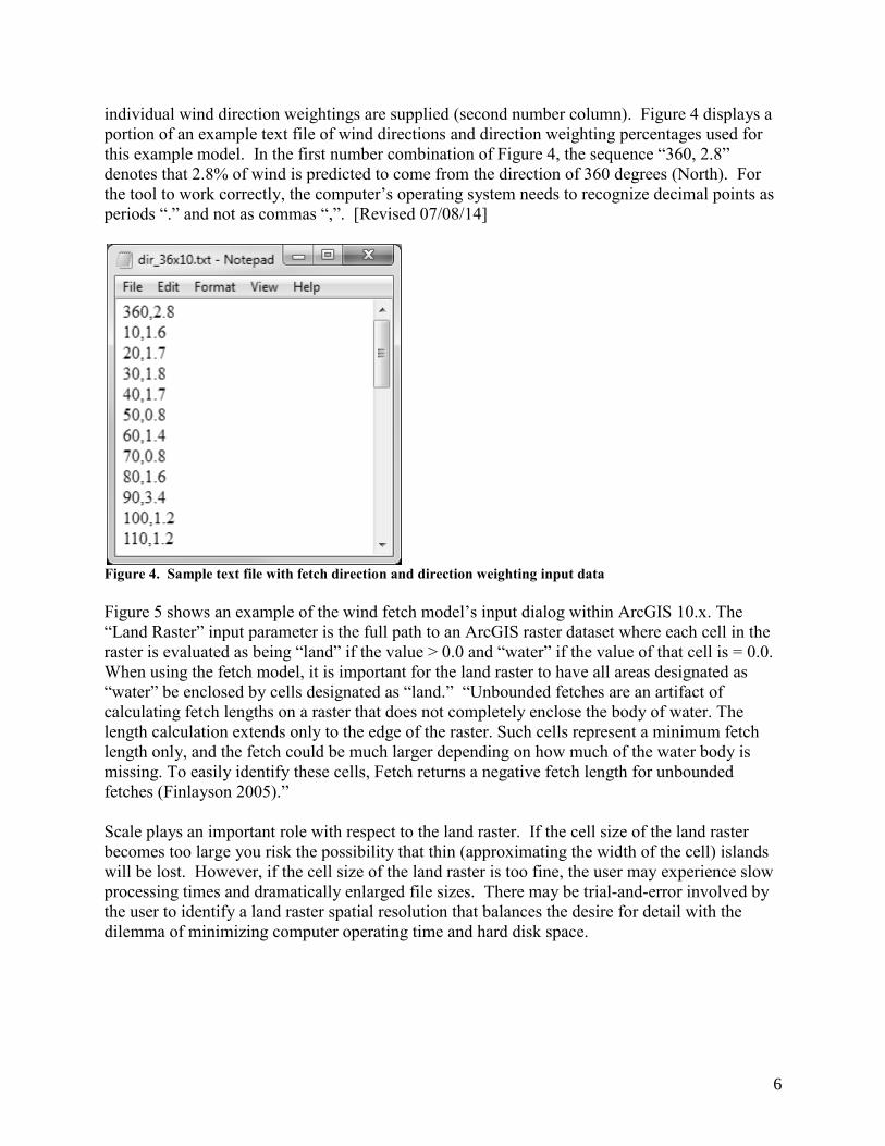
individual wind direction weightings are supplied (second number column). Figure 4 displays a

portion of an example text file of wind directions and direction weighting percentages used for

this example model. In the first number combination of Figure 4, the sequence “360, 2.8”

denotes that 2.8% of wind is predicted to come from the direction of 360 degrees (North). For

the tool to work correctly, the computer’s operating system needs to recognize decimal points as

periods “.” and not as commas “,”. [Revised 07/08/14]

Figure 4. Sample text file with fetch direction and direction weighting input data

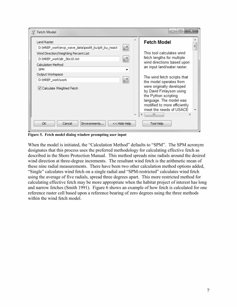
Figure 5 shows an example of the wind fetch model’s input dialog within ArcGIS 10.x. The

“Land Raster” input parameter is the full path to an ArcGIS raster dataset where each cell in the

raster is evaluated as being “land” if the value > 0.0 and “water” if the value of that cell is = 0.0.

When using the fetch model, it is important for the land raster to have all areas designated as

“water” be enclosed by cells designated as “land.” “Unbounded fetches are an artifact of

calculating fetch lengths on a raster that does not completely enclose the body of water. The

length calculation extends only to the edge of the raster. Such cells represent a minimum fetch

length only, and the fetch could be much larger depending on how much of the water body is

missing. To easily identify these cells, Fetch returns a negative fetch length for unbounded

fetches (Finlayson 2005).”

Scale plays an important role with respect to the land raster. If the cell size of the land raster

becomes too large you risk the possibility that thin (approximating the width of the cell) islands

will be lost. However, if the cell size of the land raster is too fine, the user may experience slow

processing times and dramatically enlarged file sizes. There may be trial-and-error involved by

the user to identify a land raster spatial resolution that balances the desire for detail with the

dilemma of minimizing computer operating time and hard disk space.

7

Figure 5. Fetch model dialog window prompting user input

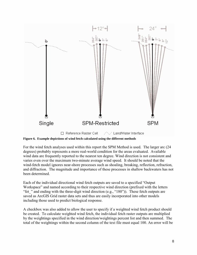
When the model is initiated, the “Calculation Method” defaults to “SPM”. The SPM acronym

designates that this process uses the preferred methodology for calculating effective fetch as

described in the Shore Protection Manual. This method spreads nine radials around the desired

wind direction at three-degree increments. The resultant wind fetch is the arithmetic mean of

these nine radial measurements. There have been two other calculation method options added,

“Single” calculates wind fetch on a single radial and “SPM-restricted” calculates wind fetch

using the average of five radials, spread three degrees apart. This more restricted method for

calculating effective fetch may be more appropriate when the habitat project of interest has long

and narrow fetches (Smith 1991). Figure 6 shows an example of how fetch is calculated for one

reference raster cell based upon a reference bearing of zero degrees using the three methods

within the wind fetch model.

8

Figure 6. Example depictions of wind fetch calculated using the different methods

For the wind fetch analyses used within this report the SPM Method is used. The larger arc (24 degrees) probably represents a more real-world condition for the areas evaluated. Available

wind data are frequently reported to the nearest ten degree. Wind direction is not consistent and

varies even over the maximum two-minute average wind speed. It should be noted that the

wind-fetch model ignores near-shore processes such as shoaling, breaking, reflection, refraction,

and diffraction. The magnitude and importance of these processes in shallow backwaters has not

been determined.

Each of the individual directional wind fetch outputs are saved to a specified “Output

Workspace” and named according to their respective wind direction (prefixed with the letters

“fet_” and ending with the three-digit wind direction (e.g., “180”)). These fetch outputs are

saved as ArcGIS Grid raster data sets and thus are easily incorporated into other models

including those used to predict biological response.

A checkbox was also added to allow the user to specify if a weighted wind fetch product should

be created. To calculate weighted wind fetch, the individual fetch raster outputs are multiplied

by the weightings specified in the wind direction/weightings percent list and then summed. The

total of the weightings within the second column of the text file must equal 100. An error will be

9

generated if the user checks this box and wind direction weightings are missing from the input

text file.

Before the model can be executed, a scratch workspace must be designated using the

“Environments…” button. It is suggested that the user select a workspace (folder) for this

parameter and not use a geodatabase (.gdb) as is sometimes suggested in the ArcGIS literature.

There have been issues with the model not operating when a geodatabase or an invalid

workspace was selected. The user should also use input files on their local hard drive and set the

output workspace as a folder on the local hard drive.

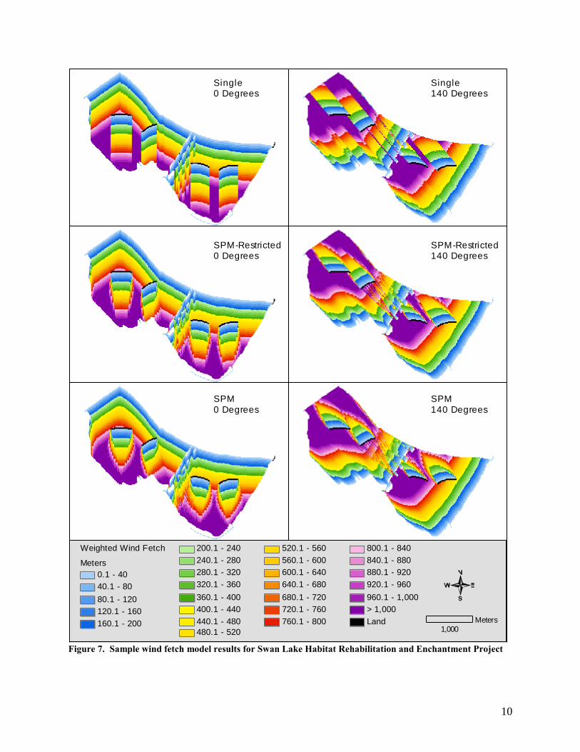
Figure 7 gives an example depiction of wind fetch calculated using the Single, SPM-Restricted,

and SPM calculation method for the Swan Lake HREP area using winds from 0 degrees and 140

degrees using the U. S. Fish and Wildlife Service (USFWS) sample management scenario.

10

Figure 7. Sample wind fetch model results for Swan Lake Habitat Rehabilitation and Enchantment Project

Single0 Degrees

SPM-Restricted0 Degrees

SPM-Restricted140 Degrees

SPM0 Degrees

SPM140 Degrees

Single140 Degrees

800.1 - 840

840.1 - 880

880.1 - 920

920.1 - 960

960.1 - 1,000

> 1,000

Land1,000

Meters

480.1 - 520

200.1 - 240

240.1 - 280

280.1 - 320

320.1 - 360

360.1 - 400

400.1 - 440

440.1 - 480

520.1 - 560

560.1 - 600

600.1 - 640

640.1 - 680

680.1 - 720

720.1 - 760

760.1 - 800

Weighted Wind Fetch

Meters

0.1 - 40

40.1 - 80

80.1 - 120

120.1 - 160

160.1 - 200

11

A validation was performed in 2008 to compare the results created using the wind fetch model

described previously with another method of calculating wind fetch, which will be termed the

measured-line method. The measured-line method of calculating fetch involved using

trigonometric calculations to create vector lines within ArcGIS from a specific point within the

area of interest. These lines were created using nine radials spread around the prevailing wind

direction at three degree increments (SPM method of fetch calculation). The point from which

the fetch was calculated was selected randomly within the area of interest, in this example Swan

Lake HREP using the USFWS proposed island design. Next, the prevailing wind direction was

then randomly selected for each fetch reference point. Lines were then generated using

trigonometry and their length was calculated using ArcGIS. Figure 8 displays the location of

each fetch reference point and the resulting lines that were generated showing the relative length

and compass direction of the lines that are used to quantify the fetch using the measured-line

fetch method.

The wind fetch was then calculated for the same area of interest using the same prevailing wind

directions using the wind fetch model. The calculated wind fetch was then ascertained by

identifying the cell within the area of interest that coincided with the reference point as

determined earlier. Table 1 shows a breakdown of the measurements calculated using the

measured-line method of fetch calculation versus the values obtained using the wind fetch

model. We see a difference of less than 10 meters in the average fetch distance using the

measured-line method and the results obtained using the wind fetch model. This is relevant since

we are basing the wind fetch model calculations off of a 10-meter cell size input dataset.

12

Figure 8. Wind fetch cell locations and prevailing wind directions used for model validation

13

10

74

1358

22

19

16

7269

6663

6057545148

172

166

169

163

160

154

151

157

148

248

251254

257

260263

266272

269

318

321

324

327

330

333

336 3

39

342

100

Meters

100

Meters

50

Meters

200

Meters

490

Meters

1,000

Meters

400.1 - 450

450.1 - 500

500.1 - 550

550.1 - 600

600.1 - 650

650.1 - 700

700.1 - 750

750.1 - 800

800.1 - 850

850.1 - 900

900.1 - 950

950.1 - 1,000

1,000.1 - 1,050

1,050.1 - 1,100

1,100.1 - 1,150

1,150.1 - 1,200

1,250.1 - 1,300

1,300.1 - 1,350

1,350.1 - 1,400

1,400.1 - 1,450

1,450.1 - 1,500

1,500.1 - 1,550

1,550.1 - 1,600

1,200.1 - 1,250

Wind Fetch (Meters)

10 - 50

50.1 - 100

100.1 - 150

150.1 - 200

200.1 - 250

250.1 - 300

300.1 - 350

350.1 - 400

1,600.1 - 1,650

1,650.1 - 1,700

1,700.1 - 1,750

1,750.1 - 1,800

1,800.1 - 1,850

1,850.1 - 1,900

1,900.1 - 1,950

> 1,950

Swan Lake HREP Area of Interest

60 Degree SPM Wind Fetch





10 Degrees

60 Degrees

160 Degrees260 Degrees330 Degrees

13

Table 1. Tabular summarization of wind fetch measurements calculated using the two different methods

Fetch Reference Angle

10° 60° 160° 260° 330°

Measured-Line Fetch (Reference Angle - 12°) 1289.42 545.48 66.05 134.82 356.59




Measured-Line Fetch (Reference Angle) 1518.06 560.03 73.10 55.85 225.17

Measured-Line Fetch (Reference Angle + 3°) 1595.90 566.77 85.51 55.41 207.63




Measured-Line Fetch (Average for 9 radials) 1180.14 564.68 82.28 63.78 243.86

Wind Fetch Model Results (Average for 9 radials) 1188.00 572.00 88.00 69.00 253.00

Difference (Meters) 7.86 7.32 5.72 5.22 9.14

Percent Difference 0.67% 1.30% 6.96% 8.18% 3.75%

A permutation test was performed to determine whether the observed pattern (the wind fetch

model results) happened by chance. Because sample sizes for the wind fetch model validation

results were small (n = 5), A non-parametric two-sample permutation test for locations was

conducted (Manly 1997). This randomization test works simply by enumerating all possible

outcomes under the null hypothesis, i.e., that no differences exist between the wind fetch model

results and the measured lines of wind fetch, and then compares the observed wind fetch model

results against this permuted distribution (based upon 5,000 permutations of the data). Results

indicated no difference between the wind fetch model results and the measured-line fetch (L =

7.053, p = 0.9744).

In Figure 9 below, the thick black line denotes the mean difference between the wind fetch

model results and the measured lines of wind fetch relative to the distribution of all possible

differences.

14

Figure 9. Results for Two-sample permutation test for locations

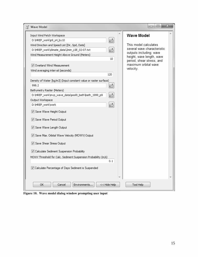
A model was constructed within ArcGIS to create several useful wave outputs. Significant wave

height, wave length, spectral peak wave period, shear stress, and maximum orbital wave velocity

are all calculated using this model. Figure 10 shows what the wave model dialog looks like for

the user. Required inputs to the model include a directory of pre-created wind fetch outputs for

the area of interest, a text file (.txt) of wind data (Figure 11), the height aboveground in meters of

the anemometer used to collect wind data, a checkbox to denote whether wind measurements

were calculated overland, the density of water, a raster with bathymetric values for the area of

interest, the threshold for maximum orbital wave velocity to use when calculating sediment

suspension probability, a workspace to store derived outputs and a checkbox to denote whether a

raster should be developed indicating the percentage of days that sediment is predicted to be

suspended based upon the maximum orbital wave velocity selected. The text file of collected

wind data is contained as comma-delimited numeric values consisting of the wind direction,

followed by the wind speed, and finally the date of data collection expressed as a two-digit year,

followed by a two-digit month, and finally the two-digit day (e.g. 020421 = April 21, 2002). The

wind data input to the wave model requires one observation for each day. [Revised 07/08/14]

15

Figure 10. Wave model dialog window prompting user input

16

Figure 11. Sample text file depicting valid input values for wind data in wave model

It is important the date values be organized like this for the model to work correctly.

The assembled wind speed data were adjusted to approximate a 1-hour wind duration, a 10-meter

anemometer height above the ground surface, an overwater measurement, and also adjusted for

coefficient of drag. These adjustments directly affect the input parameters of wave height,

period, and length. Bathymetric (water depth) data used within the model were collected from

the UMRR-EMP LTRMP (see “spatial datasets used in analyses” section for detailed

background information).

The checkbox entitled “Overland Wind Measurement” should be checked if the wind data used

within the model were collected on land and not over water which is the preferred alternative.

In the previous iteration of the wave model, the user was able to designate a single value to

represent the density of water used in model calculations. Per request of the USACE, the

functionality was added to allow the user to specify a raster surface depicting varying water

density values in addition to being able to specify a singular value. This functionality was added

to give scientists the opportunity to simulate the dampening effects of existing submersed aquatic

vegetation. Aquatic vegetation can have an effect on wave growth by dissipating waves and

thus reducing wave energy (Anderson and others 2011). It is important for the user to have a

solid understanding as to what degree the presence of aquatic vegetation may affect the density

of water before adjusting this parameter and also understand the seasonality of when certain

vegetation types are present in the water column.

The decimal number required for the input parameter “MOWV Threshold for Calc. Sediment

Suspension Probability (m/s)” is used in the calculation of sediment suspension probability (see

17

section describing Sediment Suspension Probability Analysis for more information). Any

maximum orbital wave velocity value derived that has a speed greater than or equal to the value

specified will be attributed as having sufficient maximum orbital wave velocity to suspend

sediment.

The user is given the opportunity to save the derived outputs permanently to their hard drive.

This was done to give the user the opportunity to save space, as creating several of these

floating-point raster datasets can quickly fill large amounts of disk space on the user’s computer.

Checking the checkbox labeled “Calculate Percentage of Days Sediment is Suspended” allows

the tool to automatically calculate the probability that aquatic areas within the area of interest

will have maximum orbital wave velocities sufficient to suspend sediments based upon the wind

direction and speed data used (see section describing Sediment Suspension Probability Analysis

for more information).

Before the model can be executed, a scratch workspace must be designated using the

“Environments…” button. It is suggested that the user select a workspace (folder) for this

parameter and not use a geodatabase as is sometimes suggested in the ArcGIS literature. There

have been issues with the model not operating when a geodatabase or an invalid workspace was

selected.

Wave model outputs are named according to a three digit code as a prefix and then the date the

wind data used was collected as a suffix. Sample output grid names are given below for all

potential parameters:

Wave Height = hgt_020421

Wave Period = per_020421

Wave Length = len_020421

Maximum Orbital Wave Velocity = vel_020421

Shear Stress = str_020421

Sediment Suspension Probability = vec_020421

Percentage of Days Sediment is Suspended = susp_prob

The wave model described in this report provides a simplistic method for calculating multiple

wave parameters. However, it should be noted that in many cases these simple methods have

been replaced with more realistic, and much more complex, numerical wave models. This model

provides a first-order approximation of the wave field and it should be noted that the

methodology employed neglects the effect of bathymetry on wave growth. Also, since the

method does not account for refraction or diffraction due to topography, reflection due to barriers

(including the shoreline itself), wave-wave interactions, or wave-current interactions, the results

are unrealistic and should be considered accurate only on a regional level and not on a cell-by-

cell basis (D. Finlayson, personal communication 2008.)

Wave height, period, and length inputs were derived based upon a deep-water model. There is

no single theoretical development for determining the actual growth of waves generated by

18

winds blowing over relatively shallow water (USACE 1984). Shallow water curves presented in

the Shore Protection Manual (USACE 1984) are based on a successive approximation in which

wave energy is added due to wind stress and subtracted due to bottom friction and percolation

(Chamberlin 1994). While it is realized that that the deep-water assumption will slightly over

predict wave-height, a shallow water assumption would not only make computations more

difficult, but it would also under predict wave height.

These models do not include the effect of terrestrial elevation on wave propagation. There is no

accounting for island height or the height of trees on these terrestrial land forms. As wind is

deflected up and over an island and its trees, a sheltered zone is created on the downwind side of

the island (USACE 2006). This zone is roughly 10 times the height of the island and its trees

(Ford and Stefan 1980). The value for this sheltered zone hasn’t been stated in a quantitative

fashion; however providing thermal refuge for migrating waterfowl is a desirable outcome of

island projects (USACE 2006).

The proximity of the meteorological station that the wind data is obtained from to the project

area could introduce errors due to variations in wind speed and direction caused by river valley

orientation (ie. river bluff effects). Although it is usually not practical to collect wind data

onsite, the project teams using these results should be aware of this effect.

Wave height was not tested for depth-limited breaking. If shallow bars or shoals or island

remnants exist along the fetch, they may also dissipate energy and limit the wave height.

Also, neglecting diffraction of larger waves into the protected areas within the islands will

underestimate wave energy in the protected area.

Calculating the multiple wave characteristic raster outputs is accomplished using algorithms

published in the Coastal Engineering Manual (USACE 2002) and the Shore Protection Manual

(USACE 1984). The following is a listing of variables used within these algorithms and a short

description of what they represent:

19

The first step within the wave model is to make adjustments to the wind speed data to better

approximate real-world conditions above water. Wind data used for the example analyses were

collected from the National Oceanic and Atmospheric Administration, National Climatic Data

Center (http://www7.ncdc.noaa.gov/IPS/lcd/lcd.html). Wind data used in this analysis was

collected only during the growing seasons (April – July) from 2008 to 2012. Specific wind

parameter used was the maximum 2-minute average wind speed and direction (in miles per hour

and degrees, respectively). The wind speed collected is adjusted to approximate a 10-meter

anemometer height above the ground surface using the input within the model dialog entitled

“Wind Measurement Height Above Ground (Meters)”. Since the wind speed data were collected

by the NCDC at the 10-meter elevation for these particular example locations, no adjustment is

made to the wind speed data collected. The 10-meter elevation measurement guideline is

established within the Automated Surface Observing System (ASOS) specifications. If however,

the data collected were from an anemometer at an elevation other than 10 meters the following

algorithm would have been applied:

U = observed wind speed (miles/hour)

UA = adjusted wind speed (meters/second)

z = observed elevation of wind speed measurements (meters)

t = wind averaging interval (seconds)

Ut = ratio of wind speed of any duration to the 1-hour wind speed

Cd = coefficient of drag

U* = friction velocity

λ1 = 0.0413

λ2 = 0.751

m1 = ½

m2 = ⅓

H^m0 = non-dimensional significant wave height

Hm0 = significant wave height (meters)

x^ = non-dimensional wind fetch

x = wind fetch (meters)

g = acceleration of gravity (9.82 meters/second2)

T^p = non-dimensional spectral peak wave period

Tp = spectral peak wave period (seconds)

L = wave length (meters)

um = maximum orbital wave velocity at the bottom (meters/second)

df = water depth in the floodplain (meters)

t = shear stress at the bottom (Newtons/square meter)

r = density of water (Kg/m3)

f = friction factor (assumed to be .032)

UA = U (10/z)1/7

http://www7.ncdc.noaa.gov/IPS/lcd/lcd.html

20

This approximation can be used if z is less than 20 meters (USACE 1984).

Next, the wind speed is then corrected to better approximate a 1-hour wind duration. The wind

averaging interval in seconds (t; 120 seconds for the 2-minute interval used here) is used to

compute a 1-hour average wind speed. This is done by calculating the ratio of wind speed of any

duration to the 1-hour wind speed using the equations below (USACE 2002). [Revised 07/08/14]

Most fastest mile wind speeds are collected using short time intervals, for the St. Paul and St.

Louis District examples the maximum 2-minute average wind speed is used. It is most probable

that on a national basis many of the fastest mile wind speeds have resulted from short duration

storms such as those associated with squall lines or thunderstorms. Therefore, the fastest mile

measurement, because of its short duration, should not be used alone to determine the wind

speed for wave generation. On the other hand, lacking other wind data, the measurement can be

modified to a time-dependent average wind speed (USACE 1984). Therefore, the 1-hour

average wind speed is recommended when using a steady-state model for determining wave

characteristics (Chamberlin 1994). It is important to document, however, with shorter fetches

the 1-hour averaged wind speed may be longer than needed and may result in an underestimate

of wave heights and periods. The following algorithms make this modification within the wave

model:

Next, if the checkbox labeled “Overland Wind Measurement” is checked, the wind speed is

adjusted to better approximate what the wind speed would be if it were collected over water

(Chamberlin 1994).

Finally, the adjusted wind speed is converted from miles per hour to meters per second:

This wind speed value (UA) is used in all subsequent wave model equations. It is important to

note that the wind data used in these analyses were not corrected for stability or location.

A test was performed to ascertain whether deep-water or shallow-water wave models would be

more appropriate for the analyses. In this test, if the ratio of water depth (h) to wave length (L) is

greater than 0.5 we are in an area more typically classified as deep water and the calculated wave

characteristics are virtually independent of depth, whereas if the ratio h/L is less than 0.05 we are

in an area more typically thought of as shallow water (USACE 1977). For this test the typical

water depth was calculated to be 1.6092 meters. To determine this, the UMRS Pool 9 UMRR-

U t = 1.277 + 0.296 * tanh (0.9 * log10 (45/t))

UA = UA / Ut

UA= 1.2 (UA)

UA (meters per second) = UA (miles per hour)* 0.44704

21

EMP LTRMP bathymetric data were clipped using subareas defined as part of reach planning

conducted in 2011 (USACE 2011). The subareas that encompassed Capoli and Harper’s Slough

HREP were used to calculate the mean water depth (Figure 12).

Next, the typical wave length was calculated. To accomplish this, the wave model was executed

using 28 days of wind data from 2006. These 28 days encompassed the first week of each

month during the growing season (April 1-7, May 1-7, June 1-7, and July 1-7, 2006). Upon

completion of the model, the average wave length for all 28 iterations of the model was 3.4988

meters (Table 2).

The average water depth (1.6092) was then divided by the average wave length (3.4988) to get a

ratio of 0.4898 that tends more towards what we classify as deep water (0.5). Thus, in the model

and the following analyses, the wave calculations were based upon deep water wave theory.

It is recommended that deep water wave growth formulae be used for all depths, with the

constraint that no wave period can grow past a limiting value (USACE 2002). A limiting wave

period was then calculated and compared with typical wave periods for the study areas. It was

found that the observed wave periods were less than the limiting wave period calculated using

CEM Equation II-2-39 (USACE 2002). The limiting wave period was calculated to be 3.9

seconds based upon the average water depth of 1.6092 meters calculated. It is unlikely that in

our applications the wave period would exceed this value and become limited.

22

Figure 12. Visual depiction of USACE subareas used to calculate average water depth

23

Table 2. Summarization of results used to test for deep vs. shallow water

Day Date Wind

Direction

Unadjusted Wind Speed

(U) MPH

Wave Height

(H) Meters

Wave Length

(L) Meters h/L

1 4/1/2006 320 21 0.2692 4.4784 0.3593

2 4/2/2006 340 22 0.2784 4.5167 0.3563

3 4/3/2006 330 30 0.3920 5.7217 0.2812

4 4/4/2006 300 18 0.2148 3.7027 0.4346

5 4/5/2006 150 13 0.1588 3.1032 0.5186

6 4/6/2006 140 16 0.1943 3.5205 0.4571

7 4/7/2006 10 21 0.2474 4.0030 0.4020

8 5/1/2006 150 20 0.2494 4.1930 0.3838

9 5/2/2006 260 13 0.1256 2.2573 0.7129

10 5/3/2006 300 22 0.2656 4.2657 0.3772

11 5/4/2006 300 17 0.2023 3.5573 0.4524

12 5/5/2006 320 17 0.2154 3.8597 0.4169

13 5/6/2006 210 18 0.1943 3.2237 0.4992

14 5/7/2006 190 18 0.2114 3.6171 0.4449

15 6/1/2006 320 14 0.1758 3.3710 0.4774

16 6/2/2006 330 12 0.1489 3.0008 0.5363

17 6/3/2006 40 12 0.1177 2.1935 0.7336

18 6/4/2006 150 14 0.1715 3.2668 0.4926

19 6/5/2006 200 18 0.2043 3.4546 0.4658

20 6/6/2006 280 22 0.2361 3.6343 0.4428

21 6/7/2006 330 21 0.2676 4.4357 0.3628

22 7/1/2006 300 20 0.2401 3.9877 0.4035

23 7/2/2006 270 12 0.1193 2.2298 0.7217

24 7/3/2006 30 12 0.1247 2.3767 0.6771

25 7/4/2006 340 15 0.1859 3.4514 0.4662

26 7/5/2006 300 13 0.1528 2.9512 0.5453

27 7/6/2006 220 9 0.0903 1.8721 0.8595

28 7/7/2006 200 20 0.2284 3.7205 0.4325

Averages 237 17 0.2029 3.4988 0.4898

The highest point of the wave is the crest and the lowest point is the trough. For linear or small-

amplitude waves, the height of the crest above the still-water level (SWL) and the distance of the

trough below the SWL are each equal to the wave amplitude a. Therefore a = H/2, where H =

the wave height (USACE 2002). Significant wave height is defined as the average height of the

one-third highest waves, and is approximated to be about equal to the average height of the

waves as estimated by an experienced observer (Munk 1944). Significant wave height is

calculated within the wave model according to the following formulae taken from the Coastal

Engineering Manual (USACE 2002):

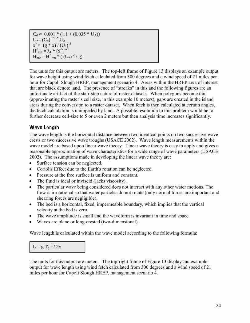
24

The units for this output are meters. The top-left frame of Figure 13 displays an example output

for wave height using wind fetch calculated from 300 degrees and a wind speed of 21 miles per

hour for Capoli Slough HREP, management scenario 4. Areas within the HREP area of interest

that are black denote land. The presence of “streaks” in this and the following figures are an

unfortunate artifact of the stair-step nature of raster datasets. When polygons become thin

(approximating the raster’s cell size, in this example 10 meters), gaps are created in the island

areas during the conversion to a raster dataset. When fetch is then calculated at certain angles,

the fetch calculation is unimpeded by land. A possible resolution to this problem would be to

further decrease cell-size to 5 or even 2 meters but then analysis time increases significantly.

The wave length is the horizontal distance between two identical points on two successive wave

crests or two successive wave troughs (USACE 2002). Wave length measurements within the

wave model are based upon linear wave theory. Linear wave theory is easy to apply and gives a

reasonable approximation of wave characteristics for a wide range of wave parameters (USACE

2002). The assumptions made in developing the linear wave theory are:

Surface tension can be neglected.

Coriolis Effect due to the Earth's rotation can be neglected.

Pressure at the free surface is uniform and constant.

The fluid is ideal or inviscid (lacks viscosity).

The particular wave being considered does not interact with any other water motions. The

flow is irrotational so that water particles do not rotate (only normal forces are important and

shearing forces are negligible).

The bed is a horizontal, fixed, impermeable boundary, which implies that the vertical

velocity at the bed is zero.

The wave amplitude is small and the waveform is invariant in time and space.

Waves are plane or long-crested (two-dimensional).

Wave length is calculated within the wave model according to the following formula:

The units for this output are meters. The top-right frame of Figure 13 displays an example

output for wave length using wind fetch calculated from 300 degrees and a wind speed of 21

miles per hour for Capoli Slough HREP, management scenario 4.

Cd ≈ 0.001 * (1.1 + (0.035 * UA))

U*= (Cd) 1/2 *

UA

x^ = (g * x) / (U*)

2

H^m0 = λ1 * (x

^) m1

Hm0 = H^ m0 * ( (U*)

2 / g)

L = g Tp 2 / 2p

25

The time interval between the passage of two successive wave crests or troughs at a given point

is the wave period (USACE 2002). Spectral peak wave period is calculated within the wave

model according to the following formulae taken from the Coastal Engineering Manual (USACE

2002):

The units for this output are seconds.

The middle-left frame of Figure 13 displays an example output for wave period using wind fetch

calculated from 300 degrees and a wind speed of 21 miles per hour for Capoli Slough HREP,

management scenario 4.

As waves begin to build, an orbital motion is created in the water column resulting in a bottom

velocity and shear stress (USACE 2006). This orbital wave velocity can be sufficient enough to

suspend unconsolidated sediments into the water column. In sufficiently deep water, the wave

particle orbital velocity at the bottom is effectively zero and sediment particles on the bed do not

experience a force due to surface wave motion (Kraus 1991). The maximum orbital wave

velocity is calculated within the wave model according to the following formula (Kraus 1991):

Maximum orbital wave velocity is based upon linear wave theory (see section describing wave

length). The units for this output are meters per second. The middle-right frame of Figure 13

displays an example output for maximum orbital wave velocity using wind fetch calculated from

300 degrees and a wind speed of 21 miles per hour for Capoli Slough HREP, management

scenario 4.

Shear stress is the drag force created on the bed by the fluid motion (Kraus 1991). Shear stress at

the bottom of the water column is understood to be an average over a wave period and is

calculated within the wave model according to the following formula (Kraus 1991):

The units for this output are Newtons per square meter. The bottom-left frame in Figure 13

displays an example output for shear stress using wind fetch calculated from 300 degrees and a

wind speed of 21 miles per hour for Capoli Slough HREP, management scenario 4.

T^p = λ2 * (x

^)

m2

Tp = (T^p * U*) / g

um = p Hm0 / (Tp sinh (2p df / L))

t = r f um2 / 2

26

Figure 13. Sample wave model outputs for scenario 4, Capoli Slough Habitat Rehabilitation and

Enhancement Project

Wave Height

Wave Length

Wave Period

Maximum Orbital Wave Velocity

Shear Stress

High: 0.5

(Meters)

Low : 0.01

High : 9.4

(Meters)

Low : 0.1

High : 2.4

(Seconds)

Low : 0.2

High : 90

(Meters/Sec)

Low : 0

High : 130,284

(Newtons/Sq. Meter)

Low : 0

Capoli Slough HREP Area of Interest

Land (Scenario 4)

1,000

Meters

27

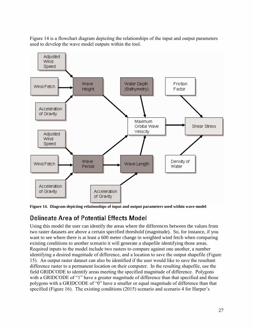
Figure 14 is a flowchart diagram depicting the relationships of the input and output parameters

used to develop the wave model outputs within the tool.

Figure 14. Diagram depicting relationships of input and output parameters used within wave model

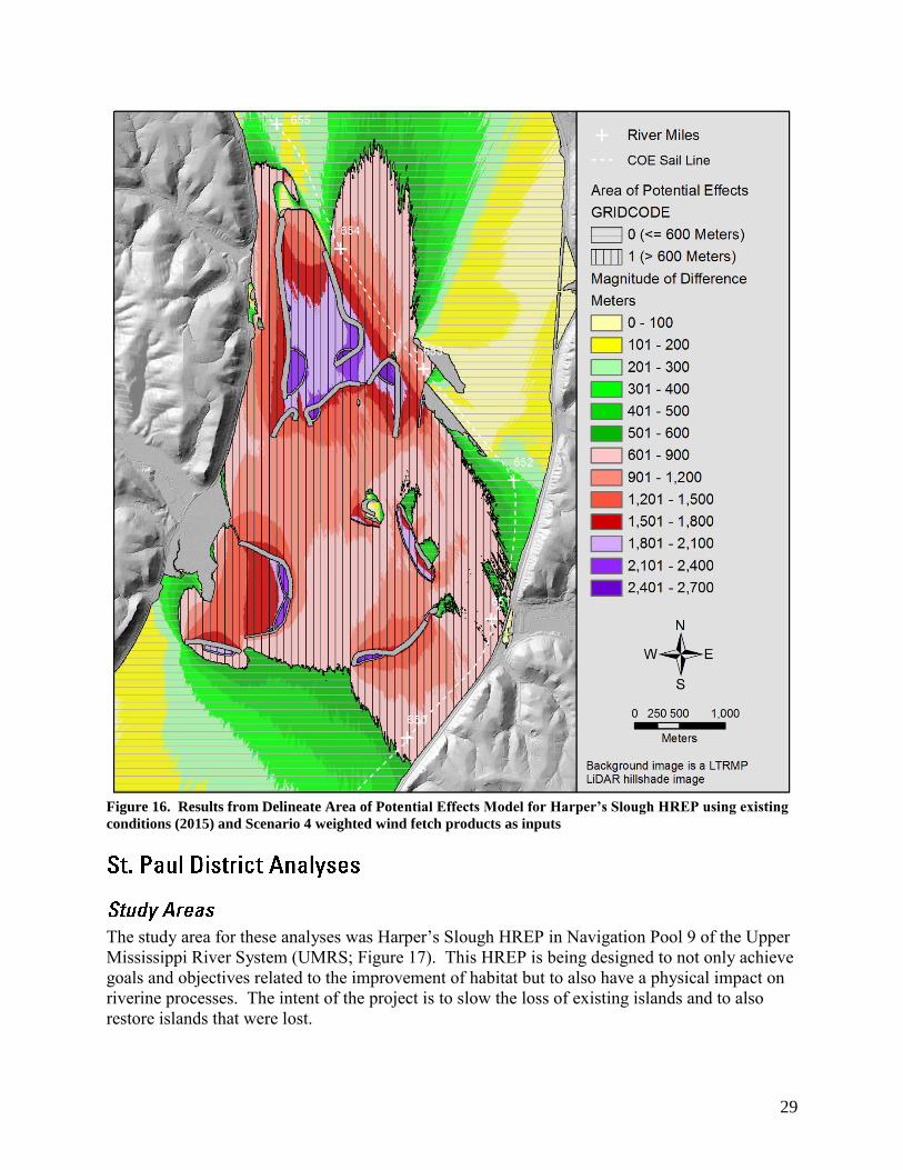
Using this model the user can identify the areas where the differences between the values from

two raster datasets are above a certain specified threshold (magnitude). So, for instance, if you

want to see where there is at least a 600 meter change in weighted wind fetch when comparing

existing conditions to another scenario it will generate a shapefile identifying those areas.

Required inputs to the model include two rasters to compare against one another, a number

identifying a desired magnitude of difference, and a location to save the output shapefile (Figure

15). An output raster dataset can also be identified if the user would like to save the resultant

difference raster to a permanent location on their computer. In the resulting shapefile, use the

field GRIDCODE to identify areas meeting the specified magnitude of difference. Polygons

with a GRIDCODE of “1” have a greater magnitude of difference than that specified and those

polygons with a GRIDCODE of “0” have a smaller or equal magnitude of difference than that

specified (Figure 16). The existing conditions (2015) scenario and scenario 4 for Harper’s

28

Slough HREP were used to develop figures 15 and 16 using an identified magnitude of

difference of 600 meters.

Figure 15. Delineate Area of Potential Effects Model dialog window

29

Figure 16. Results from Delineate Area of Potential Effects Model for Harper’s Slough HREP using existing

conditions (2015) and Scenario 4 weighted wind fetch products as inputs

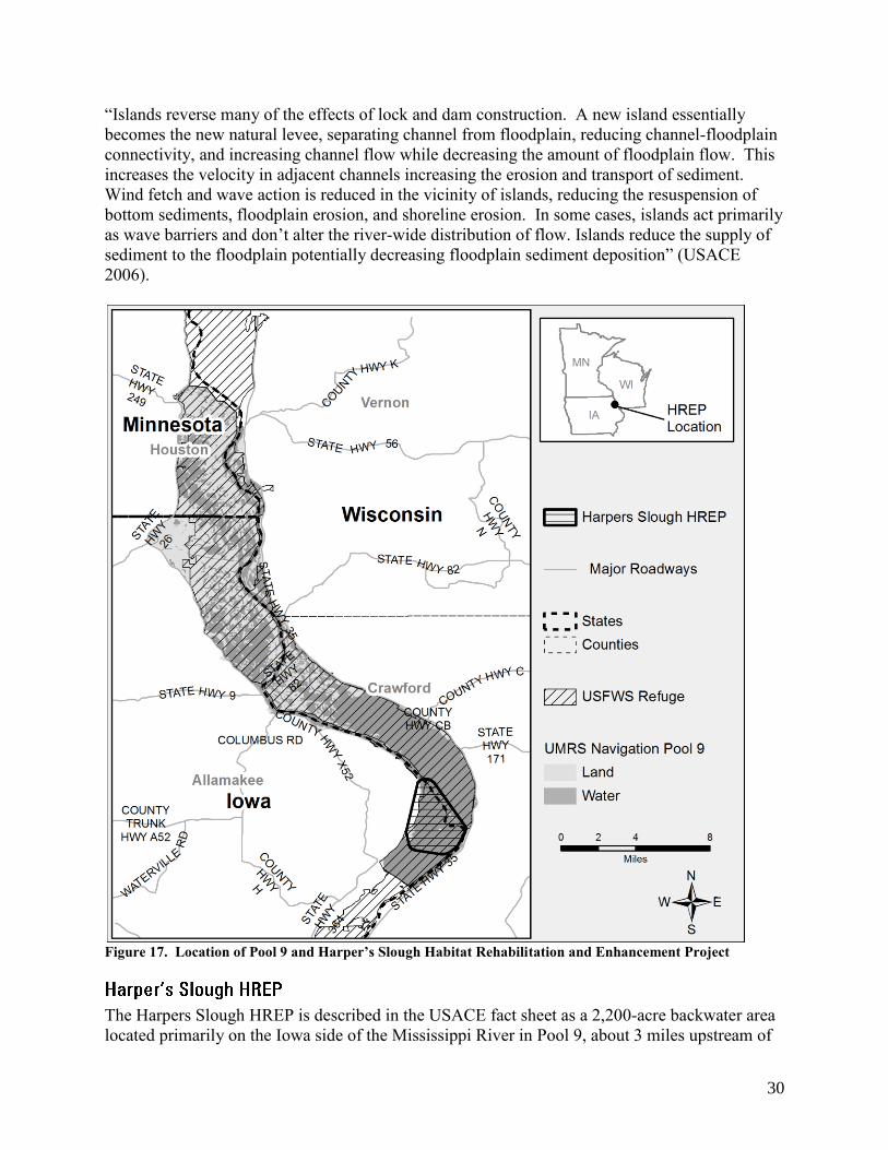
The study area for these analyses was Harper’s Slough HREP in Navigation Pool 9 of the Upper

Mississippi River System (UMRS; Figure 17). This HREP is being designed to not only achieve

goals and objectives related to the improvement of habitat but to also have a physical impact on

riverine processes. The intent of the project is to slow the loss of existing islands and to also

restore islands that were lost.

30

“Islands reverse many of the effects of lock and dam construction. A new island essentially

becomes the new natural levee, separating channel from floodplain, reducing channel-floodplain

connectivity, and increasing channel flow while decreasing the amount of floodplain flow. This

increases the velocity in adjacent channels increasing the erosion and transport of sediment.

Wind fetch and wave action is reduced in the vicinity of islands, reducing the resuspension of

bottom sediments, floodplain erosion, and shoreline erosion. In some cases, islands act primarily

as wave barriers and don’t alter the river-wide distribution of flow. Islands reduce the supply of

sediment to the floodplain potentially decreasing floodplain sediment deposition” (USACE

2006).

Figure 17. Location of Pool 9 and Harper’s Slough Habitat Rehabilitation and Enhancement Project

The Harpers Slough HREP is described in the USACE fact sheet as a 2,200-acre backwater area

located primarily on the Iowa side of the Mississippi River in Pool 9, about 3 miles upstream of

31

Lock and Dam 9. The site lies within the Upper Mississippi River National Wildlife and Fish

Refuge (USACE n.d).

The area is used heavily by tundra swans, Canada geese, puddle and diving ducks, black terns,

nesting eagles, bitterns, and cormorants and is also significant as a fish nursery area. Many of the

islands in the area have been eroded or lost because of wave action and ice movement. This

allows more turbulence in the backwater area, resulting in less productive habitat for fish and

wildlife. Harpers Slough is one of the few remaining areas in lower Pool 9 where high quality

habitat could be maintained (USACE n.d).

The proposed project would restore about 25,000 feet of islands at the upper portion of the area

using material from the backwater and near the main channel. About 8,000 feet of islands in the

lower portion of the area would be stabilized. The project would slow the loss of existing islands,

reduce the flow of sediment-laden water into the backwaters, and increase the diversity of land

and shoreline habitats (USACE n.d).

There are four goals outlined within the Harper’s Slough rough draft Definite Project Report

(USACE 2005).

1. Maintain and/or enhance habitat in the Harpers Slough backwater area for migratory

birds.

2. Create habitat for migratory and resident vertebrates with emphasis on marsh and

shorebirds, bald eagles, and turtles.

3. Improve and maintain habitat conditions for backwater fish species.

4. Enhance secondary and main channel border habitat for riverine fish species and

mussels.

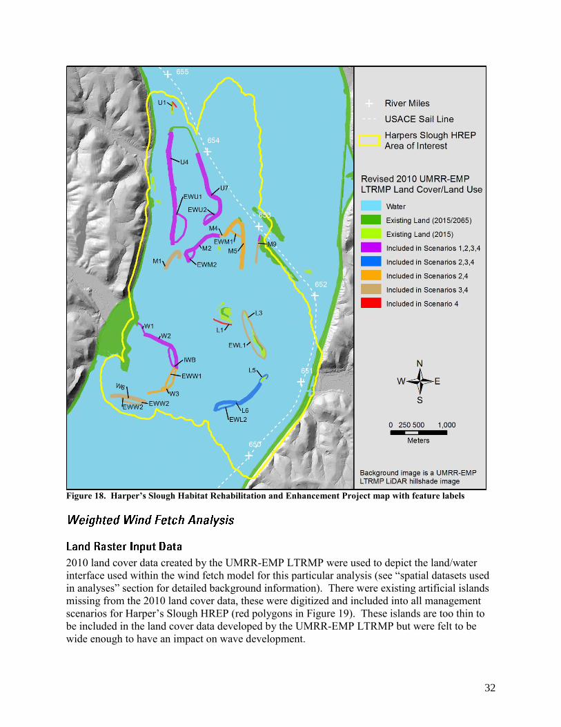
Figure 18 gives a visual representation of the Harper’s Slough HREP area using the 2010

UMRR-EMP LTRMP Land Cover/Land Use spatial data layer as a backdrop. The yellow

Harper’s Slough HREP area of interest polygon was created by calculating where the difference

in weighted wind fetch between the existing conditions (2015) and scenario 4 was greater than

600 meters using the Delineate Area of Potential Effects Model and then buffering this output by

100 meters. Features are labeled according to USACE HREP planning maps.

32

Figure 18. Harper’s Slough Habitat Rehabilitation and Enhancement Project map with feature labels

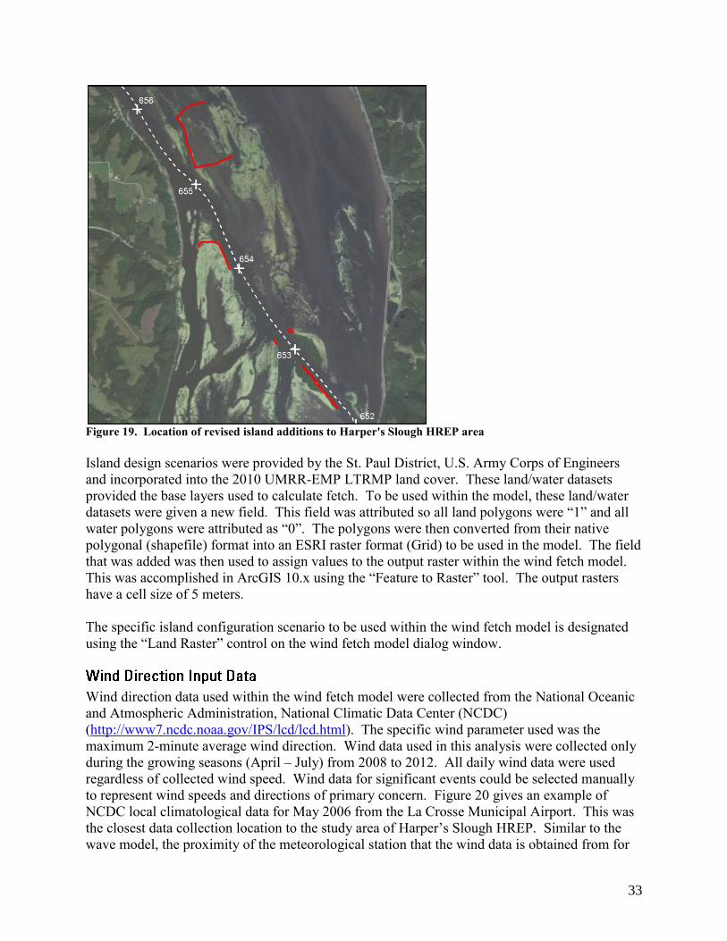
2010 land cover data created by the UMRR-EMP LTRMP were used to depict the land/water

interface used within the wind fetch model for this particular analysis (see “spatial datasets used

in analyses” section for detailed background information). There were existing artificial islands

missing from the 2010 land cover data, these were digitized and included into all management

scenarios for Harper’s Slough HREP (red polygons in Figure 19). These islands are too thin to

be included in the land cover data developed by the UMRR-EMP LTRMP but were felt to be

wide enough to have an impact on wave development.

33

Figure 19. Location of revised island additions to Harper's Slough HREP area

Island design scenarios were provided by the St. Paul District, U.S. Army Corps of Engineers

and incorporated into the 2010 UMRR-EMP LTRMP land cover. These land/water datasets

provided the base layers used to calculate fetch. To be used within the model, these land/water

datasets were given a new field. This field was attributed so all land polygons were “1” and all

water polygons were attributed as “0”. The polygons were then converted from their native

polygonal (shapefile) format into an ESRI raster format (Grid) to be used in the model. The field

that was added was then used to assign values to the output raster within the wind fetch model.

This was accomplished in ArcGIS 10.x using the “Feature to Raster” tool. The output rasters

have a cell size of 5 meters.

The specific island configuration scenario to be used within the wind fetch model is designated

using the “Land Raster” control on the wind fetch model dialog window.

Wind direction data used within the wind fetch model were collected from the National Oceanic

and Atmospheric Administration, National Climatic Data Center (NCDC)

(http://www7.ncdc.noaa.gov/IPS/lcd/lcd.html). The specific wind parameter used was the

maximum 2-minute average wind direction. Wind data used in this analysis were collected only

during the growing seasons (April – July) from 2008 to 2012. All daily wind data were used

regardless of collected wind speed. Wind data for significant events could be selected manually

to represent wind speeds and directions of primary concern. Figure 20 gives an example of

NCDC local climatological data for May 2006 from the La Crosse Municipal Airport. This was

the closest data collection location to the study area of Harper’s Slough HREP. Similar to the

wave model, the proximity of the meteorological station that the wind data is obtained from for

http://www7.ncdc.noaa.gov/IPS/lcd/lcd.html

34

use in the weighted wind fetch model could introduce errors due to variations in wind direction

caused by river valley orientation. Although it is usually not practical to collect wind data onsite,

the project teams using these results should be aware of this effect.

Figure 20. Sample National Climatic Data Center, Local Climatological Data summary sheet

Wind fetch was calculated at 10 degree increments around entire compass for each management

scenario using the wind fetch model. Figure 21 depicts the graphical breakdown of wind

direction frequencies. Of note are peaks in wind frequency from the south and the northwest.

Using the wind fetch model, these weighted individual wind fetch outputs were summed to

create a final weighted wind fetch model for each particular management scenario.

Another possible method for weighting the collected wind data instead of by the percentage of

observations from each respective direction would be to weight according to the average

intensity of the wind from each direction or some combination of the two methods.

Alternatively, you could weight only for intensities greater than a certain threshold.

35

Figure 21. Breakdown of wind directions collected for La Crosse Municipal Airport site

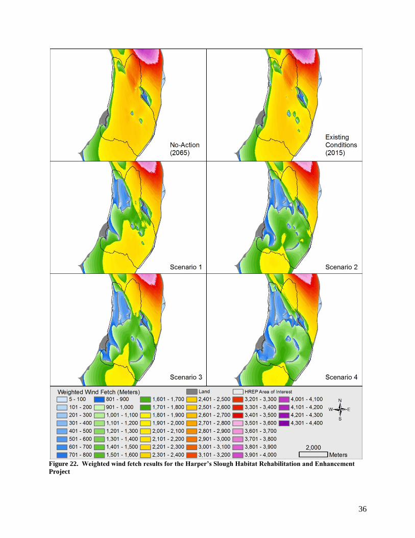
Weighted wind fetch was calculated for UMRS Pool 9 for each potential management scenario;

No-Action (2065), Existing Conditions (2015), Scenario 1, Scenario 2, Scenario 3, and Scenario

4.

Figure 22 displays the results of the weighted wind fetch analysis for each management scenario

for the Harper’s Slough HREP.

36

Figure 22. Weighted wind fetch results for the Harper’s Slough Habitat Rehabilitation and Enhancement

Project

37

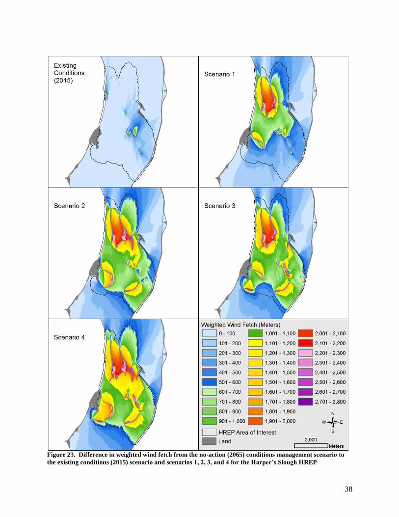
Figure 23 depicts the difference in weighted wind fetch in meters from the no-action (2065)

conditions management scenario to the existing conditions (2015) scenario and scenarios 1, 2, 3,

and 4 for Harper’s Slough HREP.

38

Figure 23. Difference in weighted wind fetch from the no-action (2065) conditions management scenario to

the existing conditions (2015) scenario and scenarios 1, 2, 3, and 4 for the Harper’s Slough HREP

39

Figure 24 shows the percent decrease in weighted wind fetch from the No-Action (2065)

management scenario to the existing conditions (2015) scenario and scenarios 1, 2, 3, and 4 for

the Harper’s Slough HREP area of interest which was defined using the Delineate Area of

Potential Effects Model. Parameters used to generate the area of interest were based upon

identifying pixels where there was at least a 600 meter difference in weighted wind fetch

between the existing conditions (2015) management scenario and management scenario 4. The

area that these selected pixels encompassed was then buffered 100 meters to create a continuous

bounding polygon.

Figure 24 Graph depicting the percent decrease in weighted wind fetch from the No-Action (2065)

management scenario to the existing conditions (2015) scenario and scenarios 1, 2, 3, and 4 for the Harper’s

Slough Habitat Rehabilitation and Enhancement Project area of interest

40

Using this weighted fetch analysis approach it is possible to quantify the amount of wind fetch

for each of the separate island design management scenarios and compare how the addition of

potential island structures may affect wind fetch. This approach took into account historical

wind data. Site-specific wind data would have been preferred but this was unavailable. The

ability to decrease wind fetch within the HREP locations would benefit these sites by lessening

the forces applied due to wave energy and thereby decreasing turbidity. With the addition of

features for each management scenario progressing from 1 to 4 we see decreases in the amount

of weighted wind fetch within both study areas.

Many factors affect aquatic plant growth. These may include site-characteristic changes in

climate, water temperature, water transparency, pH, and oxygen effects on CO2 assimilation rate

at light saturation, wintering strategies, grazing and mechanical control (removal of shoot

biomass), and of latitude (Best and Boyd 1999). According to Kreiling and others 2007, “light,

rather than nutrients, was the main abiotic factor associated with the peak Vallisneria shoot

biomass in Pool 8.” Wave action has a direct effect on water transparency. When sediments are

suspended by wave action, it causes an increase in water turbidity. High turbidity can reduce

aquatic plant growth by decreasing water transparency, thus limiting light penetration.

The sediment suspension probability analysis developed for the Harper’s Slough HREP involved

executing the wave models to calculate maximum orbital wave velocity (MOWV) outputs for

each potential management scenario and applying these MOWV values to predict sediment

suspension probabilities. According to Coops and others 1991, “maximal wave heights and

orbital velocities were concluded to be key factors in the decreased growth rates of plants at

exposed sites.”

The MOWV was calculated once daily over the growing season (April through July)

encompassing the 5-year period between 2008 and 2012 (n = 610 days). The MOWV of 0.10

meters per second was then selected to represent velocities required to suspend fine

unconsolidated sediments (Håkanson and Jansson 1983). This empirical derivation may need to

be improved upon and tested across a wider range of environments but for our purposes provides

a baseline to compare the alternative management scenarios.

Bathymetric data used in the wave model equations were obtained from the UMRR-EMP

LTRMP (see “spatial datasets used in analyses” section for detailed background information).

The bathymetric data had to be modified when calculating the MOWV for the “No Action”

management scenario. All island areas that were predicted to be lost in that scenario were given

the lowest water depth for those areas, in this example 0.01 meters (1 centimeter). A case can be

made to exclude these areas from analysis (treat as land/no data) as water depths this shallow

would most likely cause waves to break.

The next step in the analysis involved reclassifying areas within the output MOWV raster that

had MOWV values >= 0.10 meters per second with a “1” value and reclassifying areas within

the output MOWV raster that had MOWV < 0.10 meters per second with a “0” value. This was

done for all 610 raster outputs automatically by the wave model by selecting the check box to

41

“Calculate Percentage of Days Sediment is Suspended”. The tool accomplished this by summing

the individual sediment suspension probability rasters together into one raster dataset and

dividing the values by the total number of days (610) to get a percentage of days that MOWV

was at least 0.10 meters per second for each individual raster cell. This value then represents the

probability to suspend fine unconsolidated particles. Figure 25 gives a graphical illustration of

the process used to create the percentage of days sediment is suspended output using four

hypothetical raster datasets as an example.

Figure 25. Diagram explaining process for calculating percent of days capable of suspending sediments

Sediment suspension probability was calculated for UMRS Pool 9 for each potential

management scenario: No-Action (2065), Existing Conditions (2015), Scenario 1, Scenario 2,

Scenario 3, and Scenario 4.

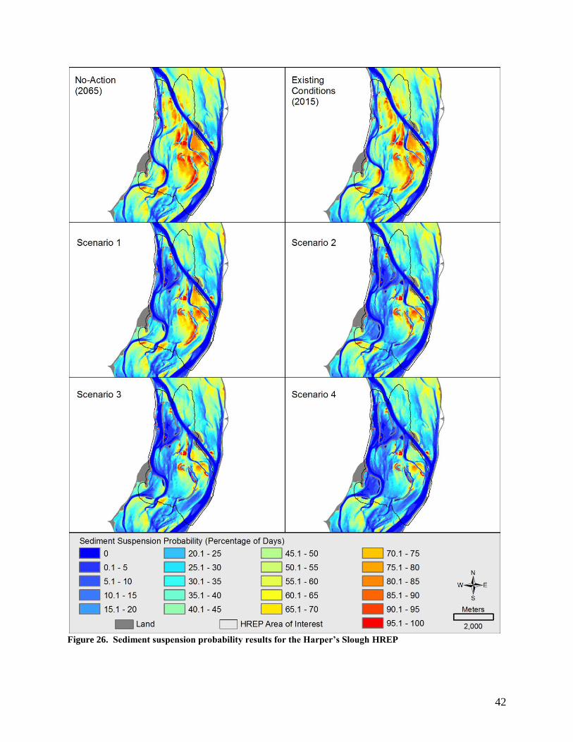
Figure 26 displays the results of the sediment suspension probability analysis for each

management scenario for the Harper’s Slough HREP.

42

Figure 26. Sediment suspension probability results for the Harper’s Slough HREP

43

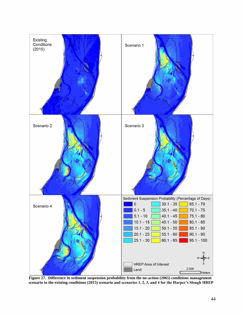
Figure 27 depicts the difference in sediment suspension probability from the no-action (2065)

management scenario to the existing conditions (2015) scenario and scenarios 1, 2, 3, and 4 for

Harper’s Slough HREP.

44

Figure 27. Difference in sediment suspension probability from the no-action (2065) conditions management

scenario to the existing conditions (2015) scenario and scenarios 1, 2, 3, and 4 for the Harper’s Slough HREP

45

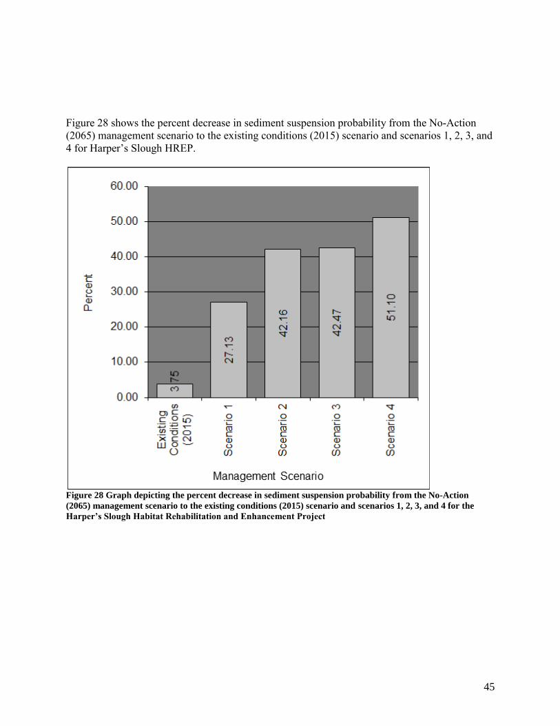
Figure 28 shows the percent decrease in sediment suspension probability from the No-Action

(2065) management scenario to the existing conditions (2015) scenario and scenarios 1, 2, 3, and

4 for Harper’s Slough HREP.

Figure 28 Graph depicting the percent decrease in sediment suspension probability from the No-Action

(2065) management scenario to the existing conditions (2015) scenario and scenarios 1, 2, 3, and 4 for the

Harper’s Slough Habitat Rehabilitation and Enhancement Project

46

This analysis provides a simplistic approach to forecasting wave effects on the suspension of fine

unconsolidated sediment particles. Based upon this approach, it is possible to depict changes in

sediment suspension probability for several potential island construction scenarios at the

identified HREP areas both with maps and summary charts. By decreasing the potential for

sediments to be suspended, there would be a decrease in turbidity. Decreasing turbidity would

increase light penetration and, therefore, create conditions more conducive to aquatic plant

growth. This approach took into account historical wind data. Site-specific wind data would

have been preferred but this was unavailable. With the addition of features for each management

scenario progressing from 1 to 4, we see decreases in the percentage of days with MOWV

capable of suspending fine unconsolidated particles within both study areas. A next step in the

process would most likely be to perform a sensitivity analysis on the MOWV identified that

causes suspension of fine unconsolidated sediments.

Upper Mississippi River Restoration – Environmental Management Program’s Long Term

Resource Monitoring Program element, as distributed by the U.S. Geological Survey, Upper

Midwest Environmental Sciences Center, La Crosse, Wisconsin

Aerial photographs for Pools 1-13 Upper Mississippi River System and Pools, Alton-Marseilles,

Illinois River were collected in color infrared (CIR) in August of 2010 at 8”/pixel and 16”/pixel

respectively using a mapping-grade Applanix DSS 439 digital aerial camera All CIR aerial

photos were orthorectified, mosaicked, compressed, and served via the UMESC Internet site.

The CIR aerial photos were interpreted and automated using a 31-class UMRR-EMP LTRMP

vegetation classification. The 2010/11 LCU databases were prepared by or under the supervision

of competent and trained professional staff using documented standard operated procedures and

are subject to rigorous quality control (QC) assurances (NBS, 1995). Online Linkage

http://www.umesc.usgs.gov/data_library/land_cover_use/2010_lcu_umesc.html

http://www.umesc.usgs.gov/data_library/land_cover_use/2010_lcu_umesc.html

47

Upper Mississippi River Restoration – Environmental Management Program’s Long Term

Resource Monitoring Program element, as distributed by the U.S. Geological Survey, Upper

Midwest Environmental Sciences Center, La Crosse, Wisconsin

Water depth is an important feature of aquatic systems. On the UMRS, water depth data are

important for describing the physical template of the system and monitoring changes in the

template caused by sedimentation. Although limited point or transect sampling of water depth

can provide valuable information on habitat character in the UMRS as a whole, the generation of

bathymetric surfaces are critical for conducting spatial inventories of the aquatic habitat. The

maps are also useful for detecting bed elevation changes in a spatial manner as opposed to the

more common method of measuring changes along transects. The UMESC has been collecting

bathymetric data within the UMRS since 1989 in conjunction with the UMRR-EMP LTRMP.

http://www.umesc.usgs.gov/data_library/aqa_feat_bath_str/bathymetry.html

We thank Keith LeClaire and Jon Hendrickson, U.S. Army Corps of Engineers, St. Paul District

for their assistance with this project. We thank Dr. Wayne Thogmartin for his assistance in the

statistical validation of the wind fetch model. This contract report was also made measurably

better by the comments of reviewers.

Anderson, M.E., J.M. Smith,, and S.K. McKay. 2011. Wave Dissipation by Vegetation.

Coastal and Hydraulics Engineering Technical Note ERDC/CHL CHETN-I-82.

Vicksburg, MS: U.S. Army Engineer Research and Development Center.

http://chl.erdc.usace.army.mil.chetn.

Best, E.P.H. and W.A. Boyd, 1999, A simulation model for growth of the submersed aquatic

macrophyte Myriophyllum spicatum L. Technical Report A-99-3, US Army Engineer Research

and Development Center, Vicksburg, Mississippi.

Chamberlin, F. 1994. Wind-generated waves in navigation pools. Report by the U.S. Army

Corps of Engineers, St. Paul, Minnesota, for the National Biological Service, Environmental

Management Technical Center, Onalaska, Wisconsin, December 1994. LTRMP 94-S001. 16

pp. (NTIS #PB95-209532)

http://www.umesc.usgs.gov/data_library/aqa_feat_bath_str/bathymetry.html

http://chl.erdc.usace.army.mil.chetn/

48

Coops, H., R. Boeters and H. Smit. 1991, Direct and indirect effects of wave attack on

helophytes. Aquat. Bot. 41:333-352.

Finlayson, D. 2005, david.p.finlayson - Puget Sound Fetch. School of Oceanography,

University of Washington, Seattle, WA. Accessed October 16, 2007, from

http://david.p.finlayson.googlepages.com/pugetsoundfetch

Ford, D.E., and H.G. Stefan 1980, Thermal predictions using integral energy model. Journal of

the Hydraulics Division, Vol. 106, No HY1.

Håkanson, L., and Jansson, M., 1983, Principles of lake sedimentology, Second edition. The

Blackburn Press, New Jersey, 316 p.

Kraus, N. Class notes for coastal sediment processes, OCEN 682, Texas A&M University and

Waterways Experiment Station Graduate Institute, 5 June to 9 August 1991.

Kreiling, R. M., Yin, Y., and Gerber, D. T., 2007, Abiotic influences on the biomass of

Vallisneria americana Michx. in the Upper Mississippi River: River Research and Applications,

v. 23, no. 3, p. 343-349.

Manly, B.F.J., 1997, Randomization, bootstrap and Monte Carlo methods in biology. Second

Edition, Chapman & Hall, New York, pp.96-97.

Munk, W.H., 1944, Proposed uniform procedures for observing waves and interpreting

instrument records. Wave Project, Scripps Institute of Oceanography, LaJolla, California.

Smith, J.M., 1991, Wind-wave generation on restricted fetches. U.S. Army Engineer

Waterways Experiment Station, Misc. Paper CERC-91-2, 25pp.

U.S. Army Corps of Engineers (USACE), 1977, Shore Protection Manual, Third Edition. Coastal

Engineering Research Center, Fort Belvoir, Virginia.

USACE, 1984. Shore Protection Manual, Coastal Engineering Research Center, Fort Belvoir,

Virginia.

USACE, 2002, Coastal Engineering Manual, Engineer Manual 1110-2-1100, U.S. Army Corps

of Engineers, Washington, D.C. (in 6 volumes).

USACE, 2005, Harper’s Slough habitat rehabilitation and enhancement project: rough draft

definite project report and integrated environmental assessment, St. Paul District.

USACE, 2006, Environmental Design Handbook, Upper Mississippi River System,

Environmental Management Program.

USACE 2011. Upper Mississippi River System Ecosystem Restoration Objectives 2009. U.S.

Army Corps of Engineers, Rock Island, Illinois. 87 pp.

http://david.p.finlayson.googlepages.com/pugetsoundfetch

49

USACE, (n.d), Harpers Slough Habitat Project, Pool 9, Iowa, St. Paul District. Accessed

September 27, 2007, from http://www.mvp.usace.army.mil/environment/default.asp?pageid=129

http://www.mvp.usace.army.mil/environment/default.asp?pageid=129

this study was funded and prepared for the u.s. army corps ... · u.s. geological survey ... wind...

Documents