this document has been reproduced from … · support the concept of a stereo electro-optical...
TRANSCRIPT

N O T I C E
THIS DOCUMENT HAS BEEN REPRODUCED FROM MICROFICHE. ALTHOUGH IT IS RECOGNIZED THAT
CERTAIN PORTIONS ARE ILLEGIBLE, IT IS BEING RELEASED IN THE INTEREST OF MAKING AVAILABLE AS MUCH
INFORMATION AS POSSIBLE
https://ntrs.nasa.gov/search.jsp?R=19800002232 2018-07-30T04:08:04+00:00Z
NASANational Aeronautics andSpace Administration
Langley Research CenterHampton Virg inia 23665AC 804 827-3965
i
110\/ 1979
RECEIVEI)
NASA STI f•AMITY.
ACCESS DEPT.
NASA CONTRACTOR REPORT 159146
FINAL REPORTSTUDY OF A
STER EO- ELECTRO-OPTI CALTRACKER SYSTEMFORTHE MEASUREMENT OF MODEL DEFORMATIONSAT THE NATIONAL TRANSONIC FACILl, fY
RICHARD J • HERTEL
a
ITT AEROSPACE/OPTICAL DIVISIONFORT WAYNE, INDIANA 46803
CONTRACT NAS 1-15629OCTOBER 1979
(NASA-CR-159146) STUDY OF A STEREO N80-10476ELECTRO-OPTICAL TRACKER SYSTEM FOR THEMEASUREMENT OF MODEL DEFORMATIONS AT THENATIONAL TRANSONIC FACILITY Final Report Unclas(ITT Aerospace/Optical Div.,) 82 p G3/'35 45845

E
t
1. Report No.159146
2, Government Accession No, 3. Recipient's Catalog No.
4. Title and Subtitle 5, Report.Date
Study of a Stereo Electro—Optical Tracker System for 25 October 19796. Performing Organization CodeMeasurement of Model Aernelastic Deformations at the
National Transonic Facility
7. Author(s) 6, Performing Organization Report No,
Richard J. Hertel10, Work Unit No.
9. Performing Organization Name and Address
ITT Aerospace/Optical Division 11. Contract or Grant No.3700 East Pontiac StreetFort Wayne, IN 46803
NASI-15629 13, Type of Report and Period Covered
Contractor Report12. Sponsoring Agency Name and Address
14. Army Project No.National Aeronautics and Space AdministrationLangley Research CenterHampton, VA
15. Supplementary Notes
16, Abstract—^
This study and report provides an analytical and experimental basis tosupport the concept of a stereo electro-optical tracker system to measuremultiple targets attached to aircraft models in the wind tunnel at theNational Transonic Facility.
The study showed that given a 0.8m x l.Om field of view and 150 }gym precisionat the model, 5-50 point illuminated targets can be acquired and t:I,,cked. Further-more, the intensities of the targets, tunnel background illumination, and systemdata rates are within reasonable bounds. A demonstration showed a time scaledsimulation of a five target tracker operating at the expected electro-opticalsignal-to-noise ratio and desired precision. The analysis and demonstration alsoshowed that targets vibrating at frequencies of 8, 50, and 200 Hz can be locatedand measured.
17, Key Words (Suggested by Author(s)) 18, r'iistribution Statement
Model Deformation InstrumentationDisplacement Measurement Systems UnclassifiedStereographic Measurement Unlimited DistributionElectro-Optical Tracker
19, Security Classif, (of this report) 20, Security Classif. (of this page) 21. No, of Pages 22, Price'
Unclassified Unclassified 79
For sale by the National Technical Information Service, Springfield, Virginia 22161
TABLE OF CONTENTS
Paragraph No. Title Page
1 .0 S24KARY..•..•.4 ....... . ...... .. .............. n••• 1
2.0 SYSTEM DESCRIPTION ............................... 32.1 Tunnel Installation•• .................. .......... 32 .2 System Operation ............... 4................. 82.2.1 Target Acquisition ................. Q. ........... . 82.2.2 Target Tracking.. .................... 4........... 142.2.3 System G'.-Ubration ............................... 202.3 System Computer ... 0.4 ......... 0....• ...... 0...... 21
3.0 ANALYSIS AND EXPERIMENTS •.•••. .... .. ••....q••••. 223.1 Optics ......................... .04•.............. 223.2 Targets ............... ............... I..,........ 243.2.1 Point Versus Finite Sized Targets ....... 1 ....... . 253.2.2 Active Versus Passive Targets .......... • .... •.... 263 . 2 . 3 Target Contrast ... . .........................A...1 283.2.4 Angular Distribution of the Target Light........ 323.3 Target Dynamics .................................. 323.4 Image Dissector Camera ........................... 343.4.1 Image Dissector Camera ... ........................ 343.4.2 Digital Interface Unit ....... ................... 343.5 'Tracker Characteristics .......................... 35
. 3.5.1 Error Dete,,Itor.. .......... 0 ...................... 353.502 Noise Equivalent Position ........................ 383.503 Measurement Cycles for Null Convergence.......... 383.6 System Precision Accuracy ........................ 423.6.1 Camera and Camera Lens Effects upon
System Precision ............................ .. 433.6.2 Target Dynamics Motion Effects upon
System Precision ............................... 463.6.3 Camera Dynamic Motion Effects upon
System Precision.......... ................... 513.6.4 Seeing Conditions ................................ 513.7 Use of Tracker Cameras for TV viewing
of the Tunnel Interior ......................... 523.8 Demonstration .................................... 553.8.1 Field of View ........... ........................ 553.802 Targets..... ...................................... 553.803 Target Acquisition....... I ....................... 553.8.4 Track and Measurement ............................ 573.8.5 Target Dynamic Simulation ........................ 57
4.0 CONCLUSIONS AND PECOMKENDATIONS .................. 604.1 Zsedits .......................................... 61
APPENDIX The Image Dissector as an Optical Tracker........ 63

LIST OF ILLUSTRATIONS
Figure No. Title Page
1 Side View of the Optical Field of View andCoordinate Systems in the Plane Yo = 400 mm........ 4
2 Top View of the Optical Field of View andCoordinate Systems in the Plane Yo = 1352 mmand Zero Angle of Attack ........................... 5
3 Camera Installation at the Test Section Wall..Y.... 7
4 System Electrical Block Diagram .................... 9
5 Program TBOSS Flow Chart ........................... 10
6 Point Tracker Operating Principle .................. 15
7 Capture Range for a 200 x 200 um Image DissectorAperture and a 35 µm Point Spread Function......... 17
8 Tracker Function Timing Diagram ............... 199 Camera Image Formats and Lens Focal Lengths for
Three Sizes of Image Dissectors .................... 23
10 Two Examples of Finite Targets ..................... 25
11 Finite Targets View at Large Angles ................ 26
12 Target Intensity Versus Background Luminance....... 30
13 LED Relative Intensity Versus Wavelength........... 31
14 Normalized Error Detector Curve Showing BrightnessUnbalance Versus Position Effect ................. 36
15 Slope of the Normalized Error Detector Curve....... 37
16 Slope Changes in the Normalized Error Curve forChanges inFocal Plane Position...... ............ 39
17 Noise Equivalent Position Versus Signal-to-NoiseRatio-. ....................... .. ............... 40
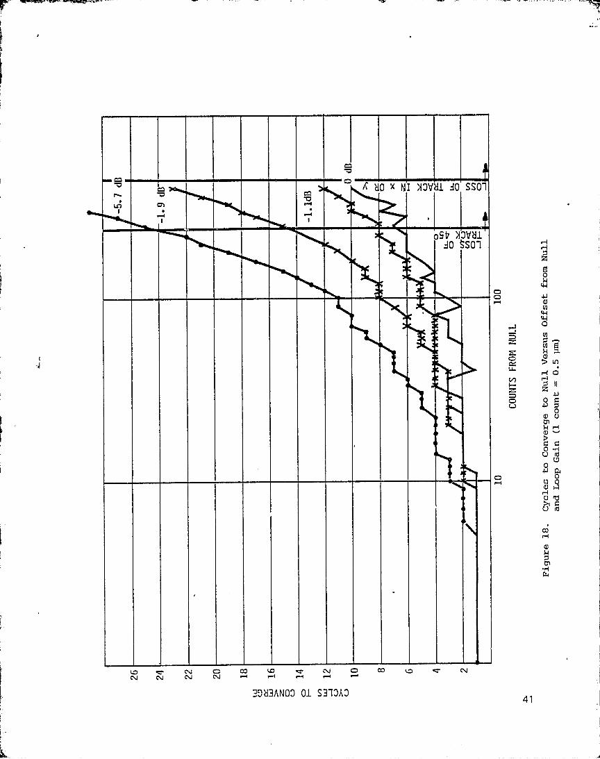
18 Cycles to Converge to Null Versus Offset fromNull and Loop Gain ................................. 41
19 10X Magnified Camera Deflection Distortion fora Camera Using 25 can Image Dissector Tube Havinga 200 11m Aperture .................................. 44
Iv
L

LIST OF ILLUSTRATIONS (Cont)
Figure No. Title Page
20 Vibration Amplitude Versus Frequency Spectrumfor Some of the Possible Vibration Modes of theWind Tunnel Model ..... 0.0. ......... 0.0..000 ...... .. 47
21 Normalized Amplitude Response Versus Number ofTargets Reduced Number of Cycles Assumes 2Xmore Light. * ....... . .................. 0...00....... 50'
22 Refraction at Test Section Window .................. 53
23 Demonstration Test Pattern... * ...............0..... 56
24 Comparison Between Timing Diagram of StereoElectro-Optical Tracker System and LaboratoryDemonstration System ............................... 58
LIST OF TABLES
Table No. Title Page
1 Target Vibration at the Model and at the Camera.... 33
2 Comparison of Stereo Electro-Optical TrackerSystem Time Scale with the Demonstration SystemTime Scale ......................................... 57
3 Vibration Simulation Frequencies and Amplitudes.... 59
v

STUDY OF A STEREO-ELECTRO-OPTICAL TRACKER SYSTEMFOR THE MEASUREMENT OF MODEL AEROETASTIC DEFORMATIONS
AT THE NATIONAL TRANSONIC FACILITY
Richard J. HertelITT Aerospace/Optical Division
1.0
SUMMARY
This study examined an electro-optical method to measure theaeroelastic deformations of wind tunnel models. The system .studied is anelectronic version of the photogrammetry method described by Brooks andBeamish- 1In place of the film, its processing and measurement, anelectronic camera system is used. Brooks and Beamish measured therecorded image positions of white target dots emplaced in the model. Theelectronic camera system does the same task in real time. It measures thecoordinates of targets focused onto its photosensitive areas.
This study shows the electronic camera system is capable oflocating, measuring, and following the positions of 5 to 50 targetsattached to the model at measuring rates up to 5000 targets per second.The targets must be either sources or efficient reflectors of light.
This study analyzed, modeled, and measured the multi-targettracking performance of one of the two electronic cameras comprising thestereo pair. Although the conditions used for this study were those esti-mated to exist in the wind tunnel at the National Transonic Facility, NASALangley, Langley, Virginia, it is emphasized tht a system of this type hasbroader application. This system can be used iii other wind tunnels wherethe environmental and vibrational conditions are less severe than NTF.This system can in fact be used for a rather wide range of thrEe dimen-sional surface contour and displacement problems.
This study considered the properties of the targets at themodel, the camera optics, target illumination,, number of targets, acquisi-tion time, target velocities and accelerations, tracker performance, andother factors affecting the measurement accuracy of target positions.
Stereophotogrammetry has been tested at Langley ResearchCenter as a means of measuring model deformations. Consideration ofstereographic transformation was not included in this study inasmuch asthe same or similar techniques used in the Langley tests will be appliedwhen using the electro-optical system.
The results of the study are presented here in terms whichdescribe the eventual measuring system; its organization, installation,and operation. A baseline system design is given with comments regarding
F
1Measurement of Model Aeroelastic Djeformations in the Wind Tunnel atTransonic Speeds Using Stereophotogrammetry, J.D. Brooks and J.K. Beamish,
[NASA Technical Paper 1010, Oct. 77.
f
s..
r "

alternatives. Some areas of technical uncertainty remain and these arenoted. An analytical and exerimental section contains the informationneeded to support the baseline design and provides the basi- for choosingamong design alternatives. This report also describes the experiments andthe demonstration, conducted at ITT-Aerospace/Optical Division, used tosupport the analytical work, to demonstrate feas.14bility of concepts, andto show working software and hardware.
g.
2

2.0 SYSTEM DESCRIPTION
The system design described in this section is a conceptualone. Most features have only been treated analytically. Some featureshave been modeled in hardware, and in a few cases experiments have beenperformed to gather supporting data.
The system described here ;assumes the use of small, self-luminous targets attached to the model. The targets are viewed by twoelectronic cameras located in the plenum of the wind tunnel behind opticalports in the test section wall. Operating modes provide for systemcalibration, target acquisition, target tracking and position measurement.Software dialog with an operator is used to select the system codes.Tunnel supervisory control is expected to identify when valid data loggingconditions exist. This system then responds to an external command andrecords target positions while the model angle of attack is slowly varied.The recorded position information is analyzed later, off line, by theexperimentor to extract the three dimensional target motions from the twocamera stereo-optical data. Provision is made for a limited amount ofquick look examination of the test data. Camera installation and sitingare important considerations in the estimated system precision andaccuracy.
2:1 Tunnel installation
Figures 1 and 2 show the general arrangement of an aircrftmodel, electronic cameras, camera fields of view and coordinate systemsused to relate three dimensional model coordinates to two dimensionalimage plane coordinates.
The aircraft model is supported by the sting and is locatedalong the center line of the tunnel. The model is -movable in pitch angle,-11 0 to +190, about a center of rotation located within the model. Themodel space coordinate system is designated (x", y", z") and has its ori-gin at the center of rotation. The model support is made as rigid aspossible but it does still bend and vibrate. The bending of the stingwith a model attacher! gives rise to rigid body motions of + 0.5 degreeamplitude in pitch, roll, and yaw about the center of rotation at frequen-cies of 8 to 50 Hz. Furthermore, the first bending mode vibrations of themodel wing are expected to fall in the range of 25 mm peak-to-peak at 20Hz to 2.5 mm peak-to-peak at 200 Hz.
The targets are sources of light, less than 500 pm diameterand flush with the surface of the model. The targets are either lightemitting diodes (LEDs) or the polished end of a fiber optic light pipe.The electrical power input to each target is 100 mW for the LEDs. Thefiber optic targets require greater power; depending upon fiber andcoupling losses. The targets emit light in all directions, and at anglesas great as 75 0 to the normal of the target. All targets must be withinthe fields of view of both cameras. These and ocher properties of targetshaving great importance to system operation are discussed further inSections 3.2, 3.3, and 3.6.
3

'OC
O Oo^ II
U4 ^wO
ca
'L! G
ri p-4
W dl
•u O E1J •rl ^
41 d
W Gam] •rqOO C
41 C)
D •-i
b O r-1
ccn U
s'a
P4
O ujO C?
N C
O WO C.7
N C
wZ-jd
p NO ctcn G
CD
m Vp
ch
H
NLA
O ^t\ I
J rj^ ^
II
O
CD
11 Ln Q1^'
O w2W
Q^1 \
LA
^ C LL
II '^O
C ^
XO\ ^ Z FQ-
\ LO U C
Tr-4 ,
(=
NO^
lD ^ }' I OC'
O / LO OW ILO Z 00
O e-i '~ C / / N Z/ r-4 UJO J Ci Lo
Zr-1
L.0J
iZ
U3L^1
LL. UX O C
l:- F-© hC J Qr-+ L1JQ ^L.
LL O
4

z
QF-OC
U-O
^ wW
uj
^Gcr
n
0
i
N
^ I
GCW
CU
f41
Oto•,Iw
^D
CV OO
W ^II
v ^
J =
Z LLJ
Wz z _z
h="UJ
N
r.Mr01
II ^
w bO 41 rl
^a^" c x
c,^d41 ro
u C 41
O E WOl OlJ
,G N C11J ,7+ r-{
Cn 00
o C7 6uG k0+
^,^1 rl 4JP b N
Saao^oO O GH u co
r
3OJLL.
Lv
5
r

There are two image dissector cameras used in this trackersystem. Figures 1 and 2 show these cameras located 400 n.m off the centerline of the model, at positions upstream and downstream of the model.Camera locations for models having wing spans 'totally i-Ad! A the field ofview are along the center line of the tunnel, agAin, upstream anddownstream of the model. In Figures 1 and 2, tho cm.ne-as lines of sightare aimed at a common point located at y" - -00 Wm. The camera pointingangles are (a,S,Y) _ (125 0 , 900 , 350 ) as shown in the figure * For thecenter line located cameras, the aim point is the center of rotation.
The system field of view is 800 by 1000 mm at the model forzero degree angle of attack and 1650 mm camera to model range. Figure 2illustrates an off center line camera installation, The field of viewcovers the fuselage and one wing of a 1.6 to 1.8 m wing span model. Theboundaries of the field of view volume are set by the 34 0 x 340 angularfield of view of the cameras and the 1550 + 450 mm depth of focus of thecamera optics. Greater depth of focus can—be obtained by increasing the fnumber of the lens at the expense of increased target illumination powerfor the game data rates. The field of view can be changed by using a dif-ferent vocal length camera lens. A shorter focal length lens gives awider field of view and greater depth of focus at the expense of measure-ment precision at the model. A longer focal length lens has the oppositeeffect. Carried to an extreme, very short focal length lenses will havegreater distortion while very long focal length lenses may have large fnumbers. Section 3.1 on optics discusses these considerations in greaterdetail.
Each camera head, camera optics, and associated electronicsare located inside temperature controlled pressure vessel. A vessel iso-lates the camera fr;m the wide range of temperature and pressure con-ditions in the tunnel. The pressure vessel has a 10 mm thick opticalquality window at one end. ThIs window withstands the static t=inelpressure. A second optical quality window in the wall of the tunnel testsection isolates the pressure vessel from the direct tunnel flow. Asketch of this arrangement i,3 shown in Figure 3.
The proper mounting of the cameras in the pressure vessel andthe pressure vessel in the wind tunnel are important Consideration--: Themounting must minimize changes in the camera-to-model vector due to vibra-tion or temperature. The mounting must also allow for temperature cortrolof the pressure vessel.
Mounting point temperatures can range from -1950C to 9500making both heating and cooling necessary. The camera and electronicspresent a 10-12 watt heat load. A satisfactory mounting is just as impor-tant as the proper target characteristics. While mounting details areoutside the scope of this study, Section 3.6 discusses the precision andaccuracy consequences of variations in the camera to model vector.
6

350
WINDOW 155 mm ^"
10 mm THICK
TEST SECTION
MM
WINDOW 60 Ran ^
10 mm THICK
0
o°ti N",/
PR'E'SSURE & TEMPERATUREISOLATION VESSEL3.5 mm WALL THICKNESS100 mm OUTSIDE DIAMETERDOES NOT INCLUDE THERMAL INSULATION
Figure 3. Camera Installation at the Test Section Wall
7
N- - -

2.2 System Operution
The system hardware is intended to operate upon the command ofthe system computer. Figure d shows a block diagr8m of the stereo-electrooptical tracker system and the interface with the tracker system computer.Each camera* rises a 16 bit, duplex, I/O channel, a 16 bit DMA channel andthe associated command and control lines. LED targets are controlled viaa serial I/O channel. If Camera Statrus is only a monitoring function,status data can be appended to the 10 bit video data. if command of thecamera housekeeping proves necessary, another I/O channel will be needed;one channel for two cameras.
The computer programs fall into three categories: 1) targetacquisition, 2) target tracking, and 3) system calibration. Singlecamera examples of the first two types of software were created during thecourse of 'this study and elements of all three typed were used for theexperiments and demonstration portions of this study.
The flow chart in Figure 5 and the following sections explainthe essential features of the system sofftwareo The twain measurementprogram is MOSS,, MOSS handle's the operah.or a?.alog and the transitionsbetween augtaisiticn and tracking. Calibral:ior is clone another programusing many portions of 11140M
2.2.1 Target Acquisition
Thte system software begins target acquisition by a call to thesubroutine ACQUIR. This subroutine turns on all the LEDs and causescamera 1 to begin a raster scan of the field of view. Subroutine SEARCHmoves camera 1 scan in x and y increments equal zu one-half the imagedissector aperture size. At each position in the field of view, thecamera measures the scene flux and returns a numerical value to SEARCH.SEARCH calculates the difference between the signal and the neighboringbackground. If the signal exceeds the background by predeterminedthreshold value a target is found. The magnitude of the threshold valueis based upon background level and signal-to-noise ratio needs of thesystem. (See Section 3.2.5 for a further,discussion.)
once a target signal is found, TGTVAL is called upon to vali-date the signal. TGTVAL checks the target list to determine if currentcamera 1 scan coordinates represent a new target or a repeat of an earlierdiscovered, target. If. no target is listed at or near the current coor-dinate, the signal-to-noise ratio above background is measured. If the
*Appendix contains a paper describing the operating principles of imagedissector tubes and cameras in tracker applications. The main text ofthis report assumes the reader has a basic understanding of this device.

9
k
CAMERA 1"'^^.. ...._...^..^ ._. ,._._. ^.....^ ._..^ e...
CQ°PETERIRE•AMP CATEO INTEGRATOR
LENS
i INPUT IRON110GE OISSECTCR TIlBE AND DIVIDE -'— AID 10 BIT ; CAMERA 1FOCUS D SHIECil0!I AASSEMBLYMAGNET I C SHIELD I
SAMPLE b HOLD
XAXIS
FOCUS
I
TRICKER I y AXIS CURRENT aPOWER
PROCESSOR
1/0 CONTROL
4 CAMERA/TRACKER CAMERA 1COIITROLLERp/A 15 BIT p/A 15 BIT 0/A R 917 D/A B BIT NO 0 SIT CMA I/O CONTR01,
04ERA 1
LATCH LATCH LATCH LATCH I
.---- OUTPUTTO CAMERA 1
DATA I ! TARGET LIST
SELECTMU% ADDER
iREGISTER — OMA ;UTPUT
TO CAMERA 1
TARGET LIST/ 017.117 OMAIHPUT
j REGISTER ; FROM CAMERA I
TRACK SCAN l
GENERATOR
TEMPERATUREICONTROL
I POWERCOt10lTIOfltNG
uux""'rlo3 STATUS CAMERA 1 STATUS'?ON[TOR
I CAI 2 --!'IPUT FROf'UMERA 2
1/0 CONTROL
Loft CAMERA 2
IPOORI,
OI41 1/0 :CNTROLCAMERA 2
6EPRODUCIBILYr,
OF
AGOUTPUT
TO CAMERA 2
IORIGINA orA DuT.11rTO CAMERA 2
jam
LFROM RFROM CAMERA 2
^—TARGET CONTROL --IN CAMERA 2 STATUS
CAMERA/TARGET SY!IC
LED
TARGETREGISTER
OUTPUT TO LETS
1BINARY TO
if LINE DECODER LED TARGET CONTROLLER 1/0 CONTROL LEOS
LED DRf'lERS
POWER
.,— __ __ __ JTO LEOS
9Figure 4. System Electrical Block Diagram
L

Figure 5. Program TBOSS Flow Chart (Sheet 1 of 3)
10

REPRODUCIBILITY OF '!TillORIGINAL PAGE', IS POOR
INITIALIZEINITIALIZE
CALL
CALLLEDON (I)
LEDON (ALL)
CALLSEARCH (2, x, y,
CALL FOUtJD)SEARCH (1, x, y,
FOUND)
FOUND FALSE
F̂OUNDFALSE TRUE
7
TRUE CALLTGTVAL (VALID, x, y,
i nT11mut nu )
P CALLTGTVAL (VALID,
X, Y, NTARG)FALSE
VALID FALSETRUE DONE
VALID FALSETRUE
0
STORE x, y inTRUE I TARGET LIST
ME NTARG = I+1STORE x, y Iil
TARGET LIST
NTARG = NTARG + 1 FALSE SCANDONE
TRUE'IDVE SAFE FALSE SCAN
DELTA DONE WRITEx= x + Ax 7 "TARGET NOT
VISIBLE TOTRUE
CAt;ERA 2"RETUR;
Figure 5. Program TOBSS Flow Chart (Sheet 2 of 3,Subroutine ACQUIR)
11
r

a
INITIALIZE
LOAD CAM,',,.2AS 1 & 2TARP:,:: INPUTREGISTERS
READ CAMERAS 1 & 2TARGET OUTPUT
REGISTERS
2FALS
ETRUEWRITE DATATO MAGTAPE
UPDATE TARGETLIST
FALSE TARGELOST
RETURN
Figure 5. Program TBOSS Flow Chart (Sheet 3 of 3, Subroutine TRACK)
12
1
r
fkFF
W- - I--•-
signal -to-noise ratio meets the system needs, the current coordinates areadded to the target list. If a target already exists at or near thecurrent coordinate, or if the signal -to-noise is less than the minimumrequired, the target list is not changed and the acquisition scan isresumed. Acquisition scan continues until the next above thresholdsignal or until the entire field of view is scanned.
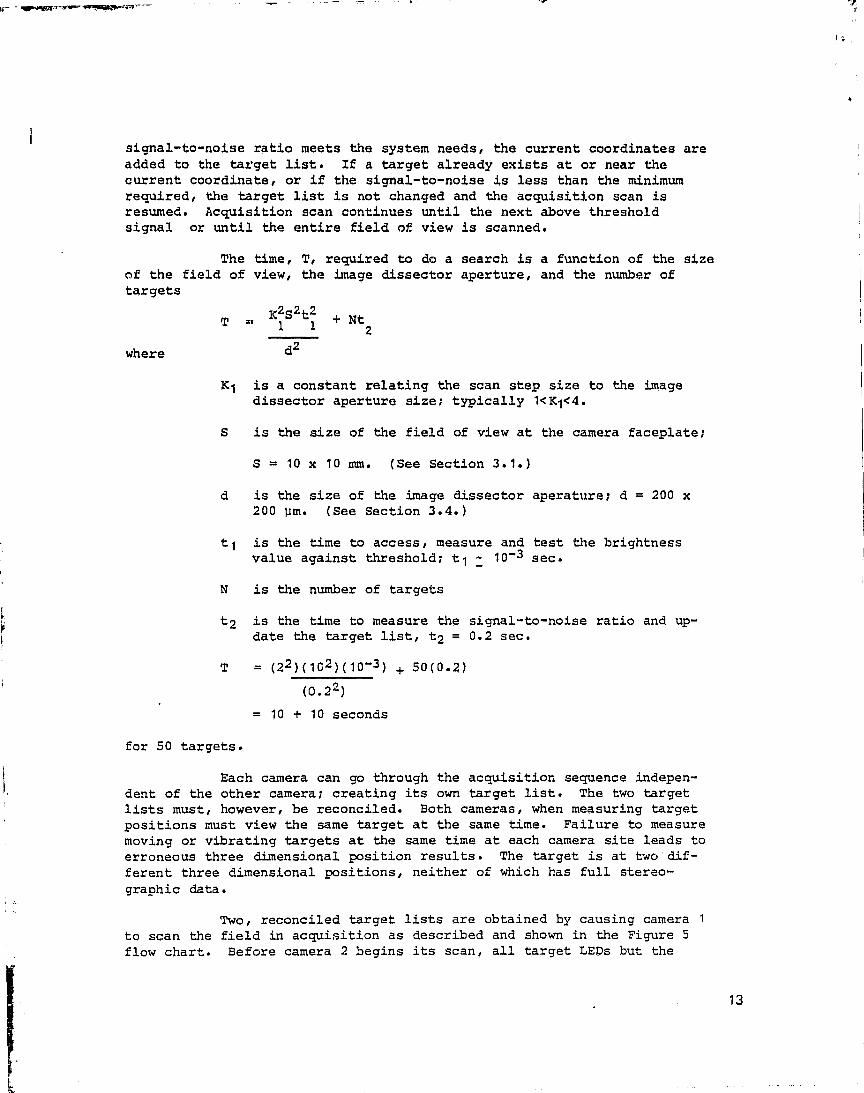
The time, T, required to do a search is a function of the sizeof the field of view, the image dissector aperture, and the number oftargets
K2S2t2T _^ 1 1 + Nt
2
where d2
K1 is a constant relating the scan step size to the imagedissector aperture size; typically 1< K1<4.
S is the size of the field of view at the camera faceplate;
S = 10 x 10 mm. (See Section 3.1.)
d is the size of the image dissector aperature; d = 200 x200 um. (See Section 3.4.)
t 1 is the time to access, measure and test the brightnessvalue against threshold; t1 = 10- 3 sec.
N is the number of targets
t 2 is the time to measure the signal -to-noise ratio and up-date the target list, t 2 = 0.2 sec.
T = ( 2 2 )(102 )( 10-3 ) + 50(0.2)
(0.22)= 10 + 10 seconds
for 50 targets.
Each camera can go through the acquisition sequence indepen-dent of the other camera; creating its own target list. The two targetlists must, however, be reconciled. Both cameras, when measuring targetpositions must view the same target at the same time. Failure to measuremoving or vibrating targets at the same time at each camera site leads toerroneous three dimensional position results. The target is at two dif-ferent three dimensional positions, neither of which has full stereo-graphic data.
Two, reconciled target lists are obtained by causing camera 1to scan the field in acquisition as described and shown in the Figure 5flow chart. Before camera 2 begins its scan, all target LEAs but the
.
13

w.
ith on the camera 1 target list are turned off. Camera. 2, via SEARCH anC,TGTVAL scans the field of view until the target is found or until the scanis complete. If no target is found, a message is printed. If a target isfound it is positively known that target i, camera 1 corresponds to targetj, camera 2. This procedure is repeated until all entries in camera 1target list have corresponding entries in the camera 2 target list.
The average time to locate the illuminated target with camera2, knowing only that it is from the camera 1 list, that it is the only oneon and all targets are uniformly distributed over the field of view, is
K2S2t2.T1 2 1d . + t
2
_ 1 (2 2 ) (10 2 ) (10-3) + 0.22 (0.22)
= 5.2 seconds.
The time for fifty targets is 260 seconds.
Knowing where to begin the camera 2 scan, at the top or bottomof its field of view will reduce this time by almost one-half:
2.2.2 Target Tracking
Following target acquisition, the system switches to thetracking mode for measurement of target positions. The computer sends thecurrent target coordinates from the target list to each of the cameras.The tracker circuitry in each camera does the position measurement inde-pendently. Figure 6 shows the sequence of steps involved. In Figure 6,the target image shown as circular area, represents the optical pointspread function seen in cross section. The ima ge dissector aperture issquare. Typical sizes are 35 um full width half maximum for the targetimage and 200 x 200 um for the aperature. Sections 3.1 and 3.3 providereasons for these sizes.
The tracker scan generator causes the image dissector camerato execute a rapid, four position track scan about the estimated targetposition. The scan amplitude in each of the two camera scan axes is typi-cally one-half the aperture size. (See Section 3.5.) The seven stepsequence positions the center of the scan pattern to the center of thetarget.* The center of the scan pattern is eventually returned to thecomputer to update the target list of each camera and to be recorded asthe target position. This sequence is repeated over and over for eachtarget.
*Actually, the scan goes to a position having equal integrated brightnessat each of the four sample positions.
1
14
t

I (Xo YO )IS THE ESTIMATED TARGET CENTER
a
1. GO TO ( X0 + OX, Yo)14EASURE BRIGHTNESS
2. GC TO ( X0 - ax, Yo )MEASURE BRIGHTNESS
3. CORRECT Xo r ! I
Xo = Xo +GX (B -1 B2[ B + B 2] L. — —
4. GO TO ( X0 , Y + AY)MEASURE BRIGHTNESS
C
5. GO TO ( X0 , Y - AY)MEASURE BRIGHTNESS
6. CORRECT YoI
Yo = Ya + Gy [B̂!3 + B
2 - B 41 r' 7
`^ 1 i7. GO TO STEP 1. 1 I
G AND G ARE CONTROL LOOP GAINS.
Figure 6. Point Tracker Operating Principle. The X and YCo-Ordinates are with Respect to the Scan Axesat the Camera
i
f
15

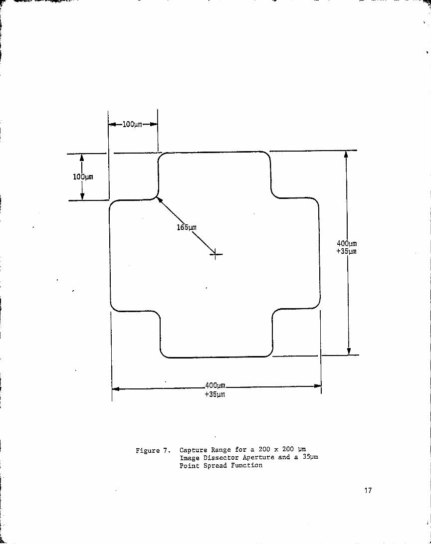
There are several properties that describe the positionmeasurement and tracking process. The First property is capture range.
1 Capture range is a vector measure of how far the targetcenter can be from the center of the track scan and stillpermit the track scan to converge upon the target centerposition. Capture range is measured ,perpendicular to thecamera line of sight. In first approximation, the capturerange falls within the area covered by the convolution ofthe track scan with the target image. For the exampledescribed here, the capture range is shown in Figure 7.*For successful operation, the target position estimate,after acquisition or when periodically returning to thetarget, must fall within the bounds of Figure 7. The sizeof the capture range sets a limit on the amplitude of thetarget vibrational motion.** For the Figure 7 case, thelimit is approximately .± 235 x V —2/2 lim or + 165 Jim (+ 21 mmat the model). In some special cases, vibrations parallelto the camera scan axes, the limit is as large as + 220 pm(27 mm at the model).
2 A second descriptive property is the number of track scancycles used to converge to the target center position. Thenumber of cycles to converge is a function of the offsetdistance between target and the track scan. Experimentresults of Section 3.5 show, for targets at the extreme ofthe capture range, 8 to 12 track scan cycles are needed.For target offsets less than 50 µm, one-fourth the aperturesize, the convergence is completed in four or fewer cycles.
3 The third property is termed convergence criterion.Convergence criterion is the maximum acceptable uncertaintyin the location of the target center. In the limit, for animage dissector tracker, the uncertainty in target positiondepends mainly upon the signal-to-noise ratio of the illu-mination falling on the photocathode. In practice otherterms such as the deflection axis D/A converter resolution,target or camera vibration, seeing conditions through theboundary and shock layers also enter. The experiments inSection 3.5 show that + 0.5 um is possible at the photo-cathode for electrical signal-to-noise ratios of 30:1 RMS.Vibration effects and seeing conditions are assessed inSection 3.6.
* The capture range at the model depends upon the range to the model, theview angle, the attack angle and the position in the field of view. Thesize at the model can be estimated for zero angle of attack at the centerof the field of view and 1650 mm range by multiplying the Figure 7dimensions by 125.
**Section 3.3 shows target loss is expected to be infrequent. The systemis programmed to skip to the next target on the list upon loss of signal.The dropout target is re-examined the next time through the target list.If all targets are lost the system switches to acquisition.
16
r r.
100um
Figure 7. Capture Range for a 200 x 200 umImage Dissector Aperture and a 35pmPoint Spread Function
17

4 A fourth property used to describe the measurement andtracking process is the time required to do one cycle ormore of the Figure 6 sequence. The tracker hardware isspecifically designed to execute the tracking scan andsignal processing algorithm. It causes the camera to scanthe target, it processes the video, corrects the scan posi-tion, and returns the corrected value to the computer.
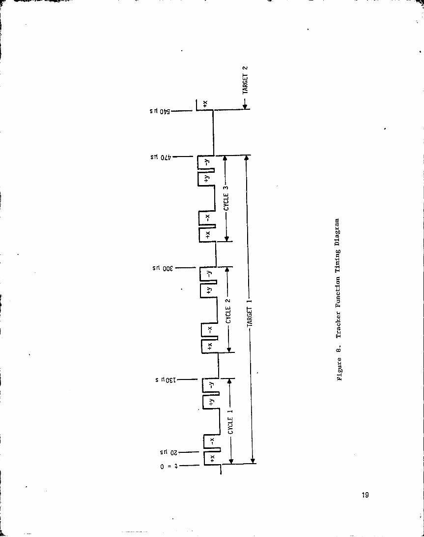
Figure 8 is a timing diagram of the tracker action for one ofthe two cameras. The camera goes to the +X scan position and integratesthe signal for 20 us. The time to store the +X value and go to the -Xscan position is 5 us. The video at -X is then integrated for 20 us. Thenext 40 us are used to update the estimate of the target X axis positionand to send the camera to the +Y scan position. The signal integrationsequence for + and -Y positions is the same as for the X position. Again,40 us are needed to update the estimate of the target X position and tosend the camera back to the +X scan position. If the camera goes to thenext target, 70 us are needed to update the estimate of the current targetY position, store X, Y and send the camera to the estimated position ofthe new target.
The time to do 1 cycle is t1 = 130 us.
The time to do n cycles on one target is
t(n) = (n) 130 ps + (n-1) 40 11s.
The time to do N targets of n cycles each is
T(N,n) = Nt(n) + (N-1) 70 us
= Nn 130 us + N(n-1 ) 40 Us + (N-1) '70 us
For example if N = 50 targets, and
n = 3 cycles per target
then t(l) = 130 us
t(8) = 470 µs
T(50,3) = 27 ms
This is a rate of 1800 targets per second. The highest ratewould be for n = 1 or 5000 targets per second.
Not all targets can be measured to an uncertainty. within theconvergence criterion in a single cycle. Neither do all targets require3, 8, or even 12 cycles. It is advantageous to make the tracker adaptive.The tracker remains at a target until the convergence criterion is met oruntil a maximum number of track scan cycles have been completed; then goesto next target.*
*This action was included in the demonstration software.
f
t
18
I
s
cv
cc
H
Sri pys -
Sri OLb--- EE,
r7lMWJVV
x
x
S ri 00£
N ^J W
VXl
x
S rim"_'
WJ
VX
Sri 07, X
0 =
00c^
AbAGSF
UC
N1aCJ
U
H
Ga
P4
19
f
2.2.3 System Calibration - The system user needs to know the trans-formation function between model space coordinates and tracker system out-put data. More specifically the user needs to know how the system differsfrom the mathematical model built into the data analysis software.
The transformation program currently being used at NASALangley for phot.ogrammetry corrects for symmetric and anti.-symmetric lensand camera distortion in a manner similar to the one used to determineviewing angles and camera distances. That is, it is a least squares coef-ficient fitting technique using }mown position of reference points. Itis thought that some reduction in computational effort could be achievedby measuring the mapping functicn of the camera, lens, pressure vesselwindow and perhaps even a test section window in calibration fixture out-side the tunnel. Section 3.6.1 describes an interpolating distortioncorrection method that is estimated to provide correction to + 0.5 pat atthe camera phot.-ocathode. The camera, lens and windows with a—correctionalgorthium and data base would then yield a system having a linear mappingfunction + 0.5 um X magnification between the object plane and camera dataoutput.
The data base is obtained by mapping the field of view of eachof the two cameras. It is assumed the distortion is a slowly changingfunction of target position within the field of view and that a finitenumber of points are sufficient to describe the function. (Section 3.6.1shows that 625 points are needed.)
The test fixture must have means to move a point source oflight about the field of view. Such a means is an array of LEDs locatedat known positions on a flat plate. There must be provisions to assurethe plate is 1650 mm from tha camera and that it is perpendicular to theoptical axis. Variations on the acquisition and tracking software gatherthe distortion map data. An analysis program is used to create thecalibration data base.
The camera and lens distortion calibration map is either pro-vided with the recorded tunnel test data or could be used to correct therecorded data before the data is given to the experimenter. Since thetracker system must operate in real time when recording data, it 'is betterto do distortion corrections ofl` line, after all data is collected.
Estimates of the optical window and the optical path seeingconditions upon the .measuxemsnt accuracy are given in Section 3.6.
It is still necessary to calibrate mm at the model as anumerical value in the software. The stereographic method being con-sidered here is a non-metric method in the projective geometry sense,This means that sizes or scale factors are not preserved and thus must becalibrated. It also means that the exact viewing angles of both camerasand their separation distance need not be known. The method l does need atleast 6 and preferably as many as 20 reference points surrounding andthroughout the volume of the combined two camera field of view. Thereference points must not be in the same plane.
l op cit page 1
20
This portion of the calibration must be done in the tunnelwith camera installed. The 0.6 to 20 reference points can be specifictargets of known location on the model. This calibrat on should be doneat test temperature and pressure as part of the data lodging process.
2.3 System Computer
The computer used in this system must be capable of supportingthe operation of the two image dissector cameras, the target LEDs, amagnetic tape recorder, a CRT operator terminal, and printer. It may alsobe desirable to have a card reader and a floppy disc unit for ease ofprogramming and program modifications.
During acquisition mode, each of the two image dissectorcameras are controlled via 16 bit, duplex .interfaces. Instruction wordsare used to set internal camera conditions and to select or not to selectthe tracker mode. LEDs operate via serial inteface. Instructions aresent only when a change in operation is required.
Two words are required for each (X,Y) coordinate. If onecoordinate is unchanged, only the one word is needed. The rate duringacquisition is 1000 coordinates per second, set mainly by software execu-tion time.
Scene flux measured at selected coordinates is returned to thecomputer as single 16 bit words. The rate is again 1000 measurements persecond.
During track*and measurement mode, the exchange between com-puter, LEDs and the two cameras occurs at a 40 K word rate. The computermust, at the same time, service the magnetic tape drive at an average 20 Kword rate, monitor the "log data" command from the outside, update thetarget list, and coordinate the actions of two cameras. The magnetic tapeunit operates 7ia a direct memory access interface. The tracker circuitryhas coordinate storage buffers containing the target list. These bufferscommunicate with the computer via direct memory access. Thus the CPUshould have ample time to observe and direct the system activities withoutbeing burdened with all the data transfers.
During calibration, the computer t'jmmunicates with the camerasas already described. The target light sources are now those on thecalibration fixtures.
The acquisition software is written in a high level languagesuch as Fortran. The driver modules for the cameras and light sources arewritten in assembly code. The track subroutine is in Fortran. The trackscan and video processing algorithm (Figure 6 sequence) is in hardware ateach camera.
No estimate has been made of memory requirements. The experi-ments and demonstration were conducted under a real time operating systemand Fortran on a computer having 24K words of memory. The main trackingprogram plus operating system used 16K words. For the experiments, thetrack scan and video processing algorithm was in Fortran.
21
i
390 ANALYSIS AND EXPERIMENTS
The design of a stereo electro optical tracker system used tomeasure aeroelastic deformations of wand tunnel models must consider thefollowing essential elements.
1. The characteristics of the targets attached to the model.
2. The illumination of the targets and the model.
3. The optical properties of the media between the model andthe electronic cameras.
4. The characteristics of the electronic cameras.
5. The effects of the tunnel environment and system installa-tion upon operation.
3.1 Optics
The field of view is 800 x 1000mm at 1650mm camera to modeldistance and zero degree angle of attack. Image dissector camera tubesare available in three sizes having photocathodes of 17, 25, and 44mmdiameter. Figure 9 shows these photocathodes, the image format size, andappropriate focal length lens.
The model can be moved +/- 450mm about the nominal 1650mmdistance. It is necessary to maintain focus over this range of distances.Operation off focus increases the radius of the point spread function ofthe lens at the image plane. The change in radius due to off focus opera-tion can be estimated by
AD.r 21 tan (a)
wherea = sin- 1 (1/2f)f = the f number of the lens.
Large f numbers provide good depth of focus but are very inef-ficient collectors of light. A compromise must be achieved between depthof focus and lens aperture.
The magnitude of ADi , the change in back focal plane position,depends upon the focal length of the lens.
A Di ^ r 1 - 1 {FL) 2CDo cl) Do(2)
for FL/Do << 1
22

44
OIMAGE 10 x 10 mm 15 x 15 mm 25 x 25 mmFORMATSIZE
LENSFOCAL 16 25 41 mmLENGTH
AD.
FOR AD =900 .091 mm .22 mm 0.60 mm0
Figure 9 • Camera Image Formats and Lens Focal Lengths for Three Sizesof Image Dissectors.. AD, is the change in back focal planeposition caused by ±450 change in object position for anobject at 1650 mm.
23
r^
H
y^ e
4
^R
P ,
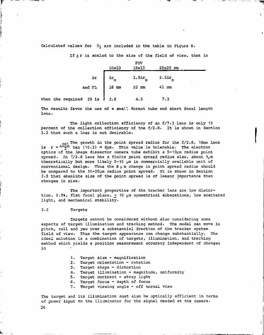
Calculated values for Di are included in the table in Figure 8.
If A r is scaled to the size of the field of view, that is
FOV10x10 15x15 25x25 mm
i Ar Ar 1.5Ar 2.5pro o o
and FL 16 mm 25 mm 41 mm
then the required f# is 2.8 4.5 7.3
The results favor the use of a sma?_, format tube and short focal lengthlens -
The light collection efficiency of an f/7.3 lens is only 15percent of the collection efficiency of the f/2.8. It is shown in Section3.2 that such a loss is not desirable.
.091 The growth in the point spread radius for the f/2.8, 16mm lensis r = 2 tan (10.3) = 8pm. This value is tolerable. The electronoptics of the image dissector camera tube exhibit a 5-10um radius pointspread. Fn 7/2.8 lens has a finite point spread radius also, about 1umtheoreti::ally but more likely 5-10 µm in commercially available unit ofconventional design. Thus the 8 u m change in point spread radius shouldbe compared to the 10-201im radius point spread. It is shown in Section3.5 that absolute size of the point spread is of lessor importance thanchanges in size.
The important properties of the tracker lens are low distor-tion, 0.5%, flat focal plane, + 10 }gym symmetrical abberations, low scatteredlight, and mechanical stability.
3.2 Targets
Targets cannot be considered without aloo considering someaspects of target illumination and tracking method. The model can move inpitch, roll and yaw over a substantial fraction of the tracker systemfield of view. Thus the target appearance can change substantially. Theideal solution is a combination of targets, illumination, and trackingmethod which yields a position measurement accuracy independent of changesin
1. Target size - magnification2. Target orientation - rotation3. Target shape - distortion4. Target illumination - magnitude, uniformity5. Target contrast- stray light6. Target focus - depth of focus7. Target viewing angle - off normal view
The target and its illumination must also be optically efficient in termsof power input to the illuminator for the signal needed at the camera.
24

r
i
3.2.1 Point versus finite sized targets. - There are two generalclasses of targets; point and finite. Point targets are not resolved as adisc image by the camera and optics. Finite targets have a definablesize, shape and even structure.
Point targets can be defined quantitatively as having an imagewhose size is less than one-third the size of the camera optical spreadfunction. The section on camera optics estimated the radius of the spreadfunction to be 10-20 um plus a 0 to S }im term for depth of focus effects.Using the dimensions of Figure 1 and a 16mm FL lens, the smallest demagni-fication is about 75 at a range of 1200mm. The size of the target,, at themodel, is therefore 2 x 750 µm/3 = 500 pm or less diameter.
Target position for point targets is measured by making foursamples in the vicinity of the target image as shown in Figure G. Thepointion of the four samples is adjusted until all have equal signalamplitude.
Numerous types of finite targets can be considered. Ingeneral finite targets require more image samples than point targetsbecause of the range of sizes and possible orientations.
Two simple examples of finite targets are the white circle ina black surround or the black and white wedge.
Figure 10. Two Examples of Finite Targets
Since the model can move in range and pitch angle, thesetargets in the extreme can look like those shown in Figure 11. A scanningmethod which is independent of these size and shape changes is a rasterwhose dimensions are greater than the maximum possible target size. Thescanned data is then used to compute the center of brightness; assuming auniform target. Tl:.rs method is time consuming if done by computer orcomplicated electronically if done by a dedicated hardware processor.
25

i
^y
Figure 11. Finite Targets Viewed at Large Angles
A less complex or time consuming method uses a circular scanpattern. The method seeks the black white edge crossings and adjusts thecenter of the scan circle until two pairs of edge crossings are each1800 apart. This method is sensitive to target rotation. The rotationmust be known or measured before proper adjustment of the scan centeroccurs.
In general, finite targets require a tracking an measurementmethod insensitive to size and shape changes. Finite targets are bestused where some useful information is conveyed by their size, shape, orpattern.
3.2.2 Active versus passive targets. - Targets can be either activesources of light or passive reflectors of light. Active point targetssuch as light emitting diodes are optically very energy efficient. Allthe energy contributes to the source intensity. Fiber optic light pipesare a bit less efficient due to losses along the fibers and at the inputcoupling. Nonetheless, optical fibers viewed end on are potentially goodtargets.
Passive point targets such as diffuse painted patterns, areoptically very inefficient in this installation. Only a small fraction ofthe incident energy is reflected to the cameras. Passive point targetscan be illuminated by a spot light that moves in step with the tracker asthe tracker moves from target to target. Such a scheme would requireeither premapping of all nominal target positions versus angle of attack,or, real time computation of illuminator pointing angles. It is stillnecessary to illuminate an area larger than the passive target since anallowance for pointing errors must be made.
The flux onto a target, at normal incidence is given by
F = g A 47 f2SNR2M2Kesle2o S At
26
F

:ate ..
where
A = 1 x 10⁻⁶ m2 , the area of a point target
f = 2.8, the focal ratio of the lens
SNR = 30, the signal-to-noise ratio needed according toSection 3.5.2
M = 125, the demagnitifcation between target and image
K = 2.3, the noise factor of the camera
e = 1.602 x 10⁻¹⁹ coulombs/electron
ElE2 = 1, reflection and lens transmission factors
S = 200 PA/lumen, the camera sensitivity
At = 20 U s, the time to make one brightness sample
F = BOA = 41T (2.8) 2 (30) 2 (125) 2 (2.3) U.6 x 10 19 ) (1) (1)
(200 x 10-6 )(20 x 10_6)
= 0.13 lumen
The target is only 1 x 10 -6 m2 in area, yet the flux is 0.13 lumens. Theilluminance must therefore be 1.3 x 10 5 lumen/m2 . This is directsunlight. For flood illumination of the 1m2 field of view at the model,this is at least 8 Kw of quartz-iodide lamps in housings with very effi-cient reflectors. For a moving spot of illumination using a 10cm2 area this is about 250 watt of quantz-iodide illumination with an f/2projector lens.
A corner cube reflector used as a passive point target' can beenergy efficient. A collimated beam of light to a corner cube isreflected back along the same path to the source. A corner cube targetdoes not exhibit the depth of focus effects previously mentioned becausethe source appears to be located at infinity. There are two majorproblems with corner cubes; size and view angle. It is not clear ifmillimeter sized cubes are available at an economical cost. Corner cubesdo not work at large angles ( 45 0 ) of incidence.
In general, active, point targets such as LEDs are preferred.
27
t—k
EC .1
E
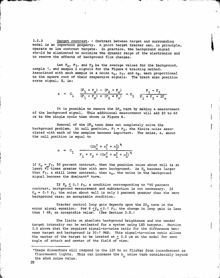
3.2.3 Target contrast. - Contrast between target and surroundingmodel is an important property. A point target tracker can, in principle,operate on low contrast targets. In practice, the background signalsho!ild be eliminated to minimize the dynamic range of the electronics andto remove the effects of background flux changes.
Let Fo, F 1 , and F2 be the average values for the background,sample 1, and sample 2 signals for the Figure 6 tracking method.Associated with each sample is a noise no , n 1 , and n2 , each proportionalto the square root of their respective signals. The track scan positionerror signal, E, is:
(F1 + Fo ) - (F2 + Fo ) F1 - F2
e - C1 (F1 + Fo) + (F 2 + Fo ) C1 F 1 + F 2 + 2Fo
It is possible to remove the 2Fo term by making a measurementof the background signal. This additional measurement will add 20 to 60Ps to the single cycle time shown in Figure 8.
Removal of the 2Fo term does not completely solve thebackground problem. At null position, F 1 = F2 , the finite noise asso-ciated with each of the samples becomes important. The noise, e, aboutthe null position is equal to
e = C1
(2no + n2 + n2) ^
F 1 + F 2 + ( 2no + n2 + n2) ^
If Fo = F1, 50 percent contrast, then the position noise about null is atleast ;2- times greater than with zero background. As Fo becomes largerthan F 1 , a still lower contrast, then no , the noise in the backgroundsignal becomes the dominant* term.
If Fo < 0.1 F 1 , a condition corresponding to > 90 percentcontrast, background measurement and subtraction is not necessary. IfFo = 0.1 F 1 , the noise about null is only 5 percent greater than the zerobackground case; an acceptable condition.
Tracker control loop gain depends upon the 2Fo term in theerror signal equation. For 0 < Fo <0.1 F 1 , the change in loop gain is lessthan 1 dB, an acceptable value. (See Section 3.5.)
The limits on absolute background brightness and the neededtarget intensity can be estimated for a system using LED targets. Section3.5 shows that the required signal-to-noise ratio for the difference bet-ween target and background is 30:1 RMS. This signal-to-noise ratio allowsthe center of the target to be located at + 0.5 um at the model for zeroangle of attack and center of the field of view.
*Image dissectors will respond to the 120 Hz ac flicker from incandescent orfluorescent lights. This can increase the b noise term considerably beyondthe shot noise value.
28

Let Io and I1 be the photocurrents entering the aperture ofthe image dissector due to the background and the target plus background.It is required that the signal-to-noise ratio of I1-I 0 be greater than orequal to 30. Since the image dissector is a shot: noise limited device,the noise in each of the two photo currents is
rekiio = Qt°^ amperes
ek2 ki 1 ^tl
amperes
wheree = 1.602 x 10 -19 Coulombs/electron
k = 2.5, image dissector noise factor
tAt = sample time, 20 us in this system.
t T1 - Io I1 - Io
SNR = _
i(ia + ii) eke (Il + Io)
At
These equations assume no ac modulation of the background. If there is acmodulation, io becomes the rms value of the modulation. As calculatedhere the equation gives the greatest do Io value that is tolerable. Thenoises are assumed to be uncorrelated and to add in quadrature.
Figure 12 is a plot of I1-Io, the required target photocurrent versus background photo current Io for SNR = 30 and At = 20 us.An additional abscissa scale on the plot shows the maximum backgroundluminance at the model for 2854 0K tungsten illumination, f/2.8 lens and a200 x 200 um aperture in the image dissector. General office illuminationis of the order of 100 lumen m-2 steradian-1.
The extra scale on the ordinate axis gives the target sourceintensity to cause the signal photo current. This intensity is based uponan f/2.8 lens and a red LED. Red LEDs produce 1 x 10 -4 watts/steradian at60 mA, current, 25 0C, and normal incidence.
Undoubtedly, there will be other sources of light used withinthe tunnel. These sources could be incandescent, fluorescent, or laser.They may even be turned ON and OFF for various reasons and will probablyoperate from the ac line. It is prudent to make the tracking system asinsensitive as possible to these sources.
There are several means available to achieve this end. First,make the targets the most intense source within the tunnel. LEDs can bepulsed to intensity levels 20-100 times greater than their dc, 250Cratings for 1 percent duty cycle at 300 Hz pulse rate. In this system,the target diode would be turned ON only when the particular target posi-tion is being measured. This will require a small amount of circuitry inthe model in addition to LED controller described in Section 2.2.
4d
29
S
It

I -NVIOMIS S11bM - AIISN31NI 3oNnos on
ter• Ln0A ^ O
ON
II
a
N
O
it
c
NO
C
C .-4O
N
NIS
Z
OJ .-d
WV
Z r-1
^ aJ
OzOcz N
V Od ^tl
e+7I
Or-1
O -4••-I r1IO A
SH3dWd - 1N3a2if10010Hd 139W
0GLnLnko
II
1JN
H
OF
N
Liu A E II
.^u
_ O U
^•G O
It̂
W w
ra U1C L .r^
V C r ZO
O
O^^!
^ G Crj
^ U C1cC .--1
p :1 pClC y .r{ m
W •r^I rz y O
^C0 •ri CO U
G1COO Ln 1:4
^ Q! NII^ca
k0 yto U H N •rlr 'O O Ov O „O o zu - co N 1= Ia Z -H oH CZ N U H -W
0--- $4 11J W CJ r-ICJ O L H Co
c0 1J y I r O0 toCU = C.
r4
HP1r4<4 n cn
N
rl
v
CD.r{
r14
30
I--r

w ;
Further reduction in system susceptibility to background illu-mination can be obtained by using narrowband optical filters on thecameras. If a filter with a passband of 50 nm centered on the 655 nm LED
emission wavelength is used, the insertion loss will be about -3 dB. Theout-of-band transmission is usually less than -60 dB.
With this kind of optical filter, background light due totungsten sources would be reduced by -13 dB, due to cool white fluorescentsources by -19 dB, but only 0 to -3 dB against HeNe laser sources.
Added discrimination against HeNe laser light can be obtainedby using a narrower bandpass and accepting a greater insertion loss orusing the less efficient green LEDs. The problem is the emission wave-lengths of red LEDs, and particularly the high efficiency red LEDs,
overlap the HeNe laser wavelength.
HIGH EFFICIENCY.>. 1.0
RED
(, GREEN I
w YELLOW
0.5
w
-r0c 500 550 600 650
HE NE
WAVELENGTH - nm
TA=25OC
GaAsP
700
750
Figure 13. LED Relative Intensity Versus Wavelength
If the narrow band optical filter does not provide sufficientdiscrimination between target and background, a phase coherent, modulatedlight system could be considered. Each of the target LEDs would be modu-lated at a frequency in the range of 5 MHz. Since the image dissectortube will pass this frequency, a tuned amplifier, phase sensitive detectorwould replace the conventional preamp. The system would accept opticalradiation within the optical filter passband having an amplitude modula-tion of 5 MHz and the proper phase relationship to a reference signal.This is a complicated approach and is an extreme but effective measure.This approach avoids the 20 to 60 u s time penalty associated withmeasuring the background. The 50 percent duty cycle of the 5 MHz modula-tion doubles the needed target intensity.
31
r's

tt _F
jt
r __ __
3.2.4 Angular distribution of the target light. - An almosthemispherical distribution of light from the target is essential.
For a flat plate at zero angle of attack the cameras viewtargets at a 350 angle from normal incidence. As the flat plate changesangle of attack, the 35 0 angle sweeps over a range of angles from 16 0 to540 . The camera has a rather wide field of view, 34 0 , therefore a nominal350 viewing angle at the center of the field of view becomes 180 to520 at the sides of the field of view for zero angle of attack and -1 0 to71 0 for 190 angle of attack. The greatest viewing angle is about 72 0 for190 angle of attack and occurs in the corner of the field of view. Iftargets are mounted on curved surfaces, this can lead to still largerviewing angles.
For a target having a Lambertian distribution, the intensityvaries as cos 0, where 0 is the viewing angle from the normal. At 0 = 70the target intensity is only osie-third of the normal valve. LEDs are notLambertian. Intensity at 70 0 is about 10 to 20 percent of on axis inten-sity. Stated differently, the brightness required for off axis viewingwill determine the target source intensity. This fact alone will likelydictate pulsed operation of the LED targets.
3.3 Target Dynamics
Vibrations of the model will occur during tests. The vibra-tions will primarily be rigid body motion of the model on the sting andbending motion of the wings. Targets attached to the model will thereforevibrate about some average position.
Table 1 gives the amplitudes and frequencies of the largest ormost rapid vibrations as provided by NASA for this study. The motions atthe model were transformed to motions at the camera image plane using theparameters
%0 = 946 mm a = 1250Yo = - 400 mm S = 900Zo = -1352 mm Y = 350
and a back focal distance of 16.157 mm. These are the conditionsillustrated in Figures 1 and 2.
Other motions of the targets, such as those which occur withangle of attack changes, take place much less rapidly or are of very muchsmaller vibrational amplitude.
All the motions given in Table 1 are excursions about anaverage position. The largest distance is 2 x 63 }im = 125 u m peak-to-peakat the camera for the 8-50 Hz yaw motion. The capture range of thetracking system should be larger than this dimension to avoid the need toperiodically reacquire a lost target. Reacquisition is time consuming insoftware. It adds to the complexity of the tracker circuitry if done inhardware. For targets at the edge of the field of view and at 190 angleof attack, the vibration amplitude at the camera can be 25 percent larger,
or 155 pm.
32
E
iL
f

3r
Table 1. Target Vibrations at the Model and at the Camera
Rigid Body ±0.50 1 8 to 50 Hz at 00 Angle of Attack
Roll Pitch Yaw Units
Target At
X" -508 -508 -508 + 5.3 mmy" -305 -610 -610 mmz" +2.2 +2.54 0 mm
Motion atCamera
z +8.3 +9.7 +63 u my 71.5 +3.8 +5.6 um
Wing Bending, Target at x" = -508, y" -610, z" = 0
Az" _ + 12.7 mm20 Hz
Az" = + 1.3 mm200 Hz Units
Motion atCamera
z +49 +4.9 Pmy +19 71.9 u m
A
C
33t
i

The capture range shown in Figure 7, for a 200 x 200 m aperturein the image dissector camera tube, has an assured capture circle of
(435 - 200) x 1a . 165 Um radius.2
Thus no need for reacquisition software or hardware is expected.
Should the vibration amplitudes be greater than those presentlyassumed, the use of a larger aperture will solve the problem at the expense ofless tolerance to background light and a greater number of cycles to convergefor large offsets.
3.4 Image Dissector Camera
The cameras used in this system are modifications of a commer-cially available image dissector crAera and digital interface unit. The hard-ware tracker is an additional item of electronics. A description of imagedissector tubes as trackers is in the Appendix.
3.4.1 lm.iq, Dissector Camera. - The camera head contains the lens, theo.image disr• ec r tube, the shielded deflection and focus assembly, voltage
divider, ryiv" j:-1% 4=uplifler. The deflection yoke driver, focus current regula-tor, ai - :t power supply and tracker hardware are contained in anelectrc'.- c—.9 iln, t L f^ ins ide bl.n vne • r_- iv ^loca
ted near 4.hC VGt4{GLGl head Ri}d V!}G p,.oqe ..^L oWa
tion vessel shown in Figure 3. Other items of housekeeping circuitry such asthe temperature controller and the digital to analog converters are alsolocated with the camera in the pressure isolation vessel.
The tube used in the camera has a 200 x 200 pm sampling aperture.The photocathode is a trialkali type, S-20 on a 7055 glass window.
The camera operates static focus and has 15 bit addressing in bothx and y axes. The addressable field of view is 12.5 x 12.5mm. One LSB in thedeflection is 0.4 um at the faceplate.
The camera requires +/-15 volts supplied by the digital interfaceunit located outside the wind tunnel.
3.4.2 Digital interface unit. - All communications between a camera andthe computer take place through this unit. It decodes the computer commandsinto operating modes of the camera, trackers and housekeeping circuitry.
An auxiliary circuit located in the model provides the on/offcontrol of the target LEDs. This circuitry occupies about 500 cm3 and
requires 7-10 watts, most used to light the LEDs.
I
34
f

3.5 Tracker Characteristics
During this study, a single camera, multi-target, point trackersystem was assembled using existing laboratory test equipment and hardware.The camera was a general purpose image dissector camera and its digital inter-face unit. A computer was programmed to run the camera. The track scan andvideo signal processing algorithm was written in software. This systemcontained many of the features that will eventua,tly be incorporated into astereo electro-optical tracker system. Section 3.8 describes the demonstrationof this system that was made at ITT-Aerospace/optical Division, Fort Wayne,Indiana. This section presents results of various measurements made on thesystemr measurements made to quantify the performance.
3.50 Error detector. - The camera plus tracker logic is a feedbacksystem. The system begins with a target position estimate, measures the errorin the estimate, and corrects the position estimate. A key element is theposition error detector. In this system it is not one discrete piece of hard-ware, but rather a term describing the results of scanning the target imageand extracting a measurement of its position relat...ve to the track scan.Figure 14 shows the measured value for the normalized error detector function
F1 (x) - F, (x)E(x)
F1 (x) + Fx (x) l y = const
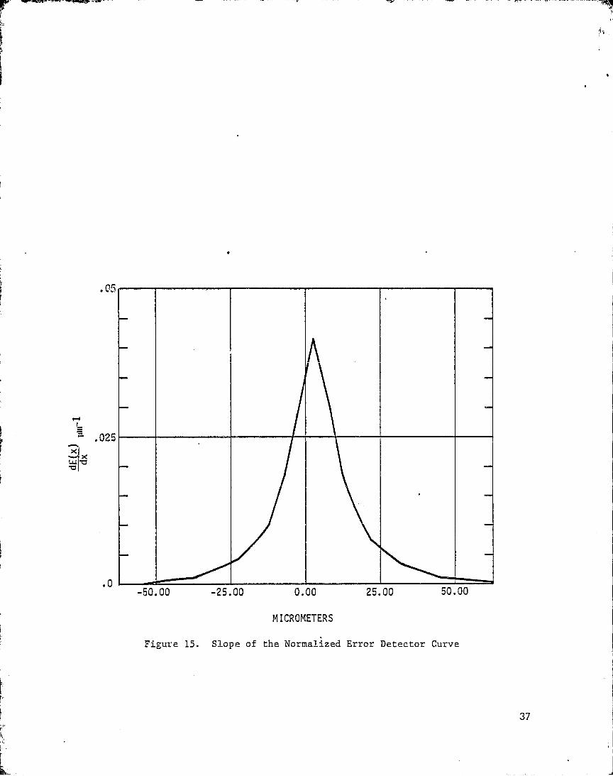
This function relates the measured imbalance in the target brightness samplesto a position difference between the center of the track scan and the centerof the target. When this distance is sufficiently small, the target positioi:is said to be measured. This curve can also be used to relate the videosignal-to-noise ratio to an equivalent position noise. The curve is linearfor small position offsets near null. Away from null the slope of the curvedecreases. For distances greater than 50 pm from null and up to the limits ofthe capture range, the slope is near zero.
The slope of the E(x) curve is shown in Figure 15 and is con-sidered to represent the sensitivity of the error detector. A change in errordetector sensitivity is also a change in loop gain of the feedback system.Changes in loop gain carry implications for system transient response and sta-bility. For the purposes of these and other experiments, the loop gain wasadjusted for best settling and minimum over shoot near null. This gainadjustment was done in software.
The non-linearity of the E(x) function for large x is a nuisance.It slows the convergence to null for large offsets as will be seen later.More troublesome are phenomena which cause the slope near null to change. Toassure system stability, the maximum loop gain must correspond to the steepestslope through null. Too high gain or an increase in slope could lead tooscillations about null. After the loop gain is set, subsequent loss of errordetector sensitivity leads to increased convergence time.
35

+1.0
E(x) .0
-50 -25 .0 Z5 Mu
MICROMETERS
Figure 14. Normalized Error Detector Curve ShowingBrightness Unbalance Versus Position Effect.
36
. 05
.025xw^1
.0-50.00 -25.00 0.00 25.00 50.00
MICROMETERS
Figure 15. Slope of the Normalized Error Detector Curve
-
37
rE

F
e
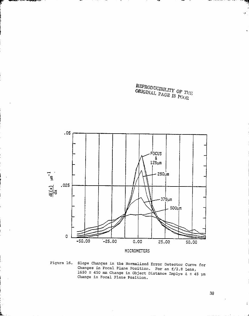
The :shape of the error detector curve and consequently it.s slopenear null is affected by changes in the target image. A larger image willcause a reduction in slope. Magnification changes between the model and thecamera or depth of focus effects can cause changes in the size of the targetimage. The design approach has been to make the target image smaller than theoptical point spread function and thereby minimizing the magnificationeffects. The depth of focus effects have been minimized by use of a f/2.8lens, see Figure 16. A slower lens gives a greater depth of focus but at theexpense of target intensity. There is some advantage to creating a largerpoint spread function. A larger point spread will tend to linearize the E(x)function over a greater range and thereby reduce the number of cycles neededto converge to null. However, such action .requires the optical signal-to-noise ratio be increased in order to hold the same noise equivalent positionerror.
The targets form an important part of the system design and havean effect upon performance. The experimenter and model builder will need toconsider this fact.
3.5.2 Noise equivalent position. - Noise equivalent position is a fun-damental property of the system relating to measurement precision. it is away of expressing system noise sources in terms of a single position uncer-tainty at the faceplate of the camera or at the model. Some of the importantnoise sources are the shot noise in signal, the D/A and A/D quantizationnoises, and camera and lens distortions. The effects of vibration and seeingconditions are treated sepdrately under Section 3.6 on accuracy. Camera andlens distortion are presumed to be fixed and measurable.
Figure 17 is a graph of position uncertainty as a function ofsignal-to-noise ratio of the target signal. The target signal includes bothshot noise an$ A/D quantization noise. The position uncertainty is asymptoticto + 1/2LSB* or + 0.25 um. A signal-to-noise ratio of 30:1 yields a + O.SUmposition uncertainty. This curve resulted from measured performance on thehardware and software used for the demonstration.
3.5.3 Measurement cycles for null convergence. - As mentioned in 3.5.1,the error detector function is non-linear away from null. This implies thatseveral track scan measurement cycles are needed. Each cycle contributes,an increment of correction, as the error i:_ nulled to the noise limit.
Figure 18 is a plot of the measured number of cycles needed toconverge +1LSB or + 0.5 pm of the null position versus the distance from null.The 0 dB gain condition represents no change from the loop gain that providesthe fastest settling and minimal overshoot about null. The other curves aredeliberate reductions in the loop gain to illustrate the effect upon con-vergence time. The time to do n cycles is
to = (n) 130 µs + (n-1) 40 us
based upon the Figure 8 timing diagram.
*The demonstration system provided this data and used 13 bit deflection over4.1 mm or 0.5 }=/count. The system described in Section 3.4.1 is the oneto be used in the tunnel installation. It will use 15 bit deflection over12.5 mm or 0.4 um/count. The signal-to-noise ratio dominates the + 0.5umposition uncertainty.
38
A
k
"I
RP!'PROD UCR3ILITyOFO,RIG1NAL PAGB 2'1-1
IS PD()h
FOCUS
125µm
.OE
E 250µm
.025x xw^
37511m
500um
0-50.00 -25.00 0.00 25.00 50.00
MICROMETERS
Figure 16. Slope Changes in the Normalized Error Detector Curve forChanges in Focal Plane Position. For an f/2.8 Lens,1650 y 450 mm Change in Object Distance Implys A y 45 µmChange in Focal Plane Position.
39

NCWHwr0CUr-^
2
1
10 30 100
SNR
Figure 17. Noise Equivalent Position Versus Signal to Noise Ratio(1 Count = 0.5 um)
{I
40
JJzCCLt.Nrz0U
z5O4
a^N
44.1O
N
^4 r.OP LO
r-1 C7
z+-)
O C:4J ^$
OO U}1 r^
UDG GO •rl
U ^C7
O
ON O'U ^1
r-1U FO>1 GU rtf
p
a0
Cr^
UNGQ^
W
n
nc
7 a0 x NI Novt 30 SS03b
0st Nova30 ^SO'1
F
...
i
l0 C' N O CO l0 -::r N O W In <T NN N N N r+ r•-1 rW r-4
39EAN00 Ol SMAO
E.Cs
41

I14
The stepped, even sawtooth appearance is due to a aeon-linearchange in loop gain implemented in the software tracker used for these tests.When the position correction is calculated to be greater than 20 counts or 10um, the correction actually made is 40 counts or 20um. This scheme initiallyovershoots but cuts the number of cycles in half.
Since a target can be expected anywhere within the capture rangewhen the tracker returns to re-examine its position, quite a few cycles couldbe required to reconverge some targets. Tracker hardware design should allowa degree of adaptation. It should require the target measurement cycles tocontinue until -the correction value is less than or equal to +1LSB or untilsome maximum number of cycles have been executed. This will assure full measure-ment precision with minimum time expenditure, plus a means to identify lessaccurate measurements, yet not be trapped forever while attempting to convergehigh amplitude, rapidly vibrating targets.
3.6 System Precision and Accuracy
This section discusses the precision and accuracy of the systemconcept. Precision is taken to mean the ability to determine small changes ina target position using a stable, repeatable scale of measure; a scale that isconsistent throughout the field of view. The accuracy of the system is takento mean the degree of agreement between the system scale of measure and anexternal absolute scale such as millimeters at the model. If good systemdesign yields a sufficiently precise system, then a suitable calibrationmethod and data reduction should give a commensurate accuracy.
The limitations upon the precision of the system will be coveredby examining the contributions of the-several parts. The major divisions arethe camera and its lens, the dynamical motions of the targets, the dynamicalmotions of the camera installation, and the seeing conditions.
Ideally the results should be described in terms of dimensions atthe model. However, there is no single factor that relates incremental posi-tion changes at the model to image changes at the camera. The relationshipdepends upon the location of the target in the field of view, the viewingangle of the camera, the focal length of the lens, the range between model andcamera, the angle of attack of the model, and vector direction of the positionchange.
For estimation purposes the model can be considered a flat plateat zero degrees angle of attack, 1650mm range and viewed using a 16mm focallength lens. For a target located at or near the center of the field of viewand viewing angles (asy) _ (125,90,35) (See Figure 1), the model to image rela-tionship can be described by 3 de-magnification numbers, Mx" My" Mz".
MODEL CAMERASPACE SPACE FACTOR
Ax" _ + lmm 6x = + 8.Oum M:%" = 125A y" + lmm Ay + 9.8um My" = 102A z" + lum Az + 5.6um Mz" = 178
42
r.

3.6.1 Camera and camera lens effects upon system precision. - The cameraand lens act in several ways to limit the system precision. The simplestlimitation to understand is the one due to small but finite sized deflectionincrements. The demonstration system, described in Section 3.8, used 13 bitdeflection D/A converters over a 4.1 x 4.1 mm field of view. The minimum stepsize was 0.5 um at the camera faceplate. The system design concept presentedin this report uses a 10 x 10 mm working field of view. Fourteen and 15 bitconverters provide 0.8 to 0.4 Um increments respectively while covering a 12.5x 12.5 mm scanable field of view. Such converters are available for thecamera.
D/A converters and cameras have temperature dependencies whichaffect the size of the area scanned and the stability of the scan centerwithin the field of view. A change in scan size is equivalent to a change inscale factor at the camera faceplate. The magnitude of the error is equal tothe distance from the center of the field of view times a +20 ppm/ oC tem-perature coefficient. Values range from zero at the center to +0.12 µm/ oC atthe edge of the field of view.
The centering term is +10 ppm/ pC of the full scale size or +10 x10 -6 x 12.5 mm = +0.12 um/oC. All coordinates within the field of view areequally affected by this factor. The pressure isolation container used tohouse the cameras must have tem perature control because of the -1950C to 950Ctunnel environment. The temperature coefficients require the control of thetemperature, at certain key locations in the container, be the order of plusminus one to two degree Celsius.
The mechanical packaging of the camera and its lens must preventshifts of the tube relative to the focal plane or coil system. The need isfor less than +0.5 um instabilities, a value consistent with the needs ofprecision star trackers used for space flight.
The camera and lens both introduce distortions of the field ofview. Figure 19 shows the magnified distortion of an uncorrected imagedissector camera without lens. It is assumed the lens distortion is com-parable or less in magnitude. The dotted boxes are on a 1 mm grid and cen-tered on the true position. The distance from the center to the side of thesmaller boxes is + 25 li m; + 40 pm for the larger boxes.
This distortion is in principle correctable using a lookup tableand interpolating between table entries. A key question is how large must thetable be in order to correct + 0-511m?
Consider a group of four boxes in Figure 19 whose centers aredenoted by A, B, Cr D. The distance between AB is 2 mm and the same holds forCD. Assume the x and y position errors are known by measurement for the fourpositions. The position error for any point E inside the retangle ACED canthen be calculated by interpolation using
EX = k 1 Cx + (1-k 1 ) DxE = k2Ay + (1-k2 ) By
43
E

I J':wo55
X-RX13 Mt
71
V. ...
. ... )
..... .... .... .. .....
.......... .......... ..... ..........
057809
8007846-4122 20K
07-RUG-78
Figure 19. 1OX Magnified Camera Deflection Distortion for a CameraUsing 25 mm Image Dissector Tube Having a 200 pm Aperture
44

A • B • 2 mm
D •
E (kl
C
•
2 mm
where the subscript denotes the component of the error and k 1 , k2 is the posi-tion of point E from C and A respectively. The interpolation is leastaccurate when E is farthest from the four reference points. This occurs whenE is at the center or k, = k2 = 0.5. E at the center is the case illustratedby Figure 19.
Analysis of the 157 points in Figure 19 showed that Ex andE calculated by interpolation different from the measured values for Ex andE by + 2 µm typically and + 4 µm at the greatest.
Assume the interpolation error is proportional to the area of theACBD cell. Then a + 0.5 µm interpolation error can be achieved using( 2) 2 x 0.5/4 = 0.25 mm 2 , 0.5 x 0.5 mm cell. The 12.5 x 12.5 mm will bemapped to a sufficient density using (12.5) 2/(0..25) = 625 points.
Changes in target light level and background do not directlyaffect the accuracy as long as a minimum signal-to-noise ratio exists.Section 3.5 shows SNR = 30 for +0.5 µm error. A signal-to-noise ratio test isincluded in the target acquisition routine to ensure sufficient target inten-sity for the desired measurement accuracy. The SNR test would add about 0.1second per target to the acquisition time.
In summary the camera, lens and target intensity contributions tothe loss of measurement precision are:
Deflection Step Size: +0.4 µm
Temperature Coef of FOV Size: +0.12 µm/oC at edge0 at center
Temperature Coef of Center Offset: ±0.12µm/OC
Mechanical Package: +0.5µm
Corrected Lens and DeflectionDistortion: +0.511m
Signal-to-Noise Ratio: +0.5µm 45
^I

3.6.2 Target dynamic motion effects upon system precision. The targetsare moving while the cameras attempt to measure their positions. Section 3.3cited some of the amplitudes and frequencies that might be expected. Figure20 shows an envelope of possible amplitudes and frequencies for a variety ofmodels. The amplitude is given in µ m at the faceplate of a camera.A scale along the right side shows the n tuber of tracker cycles needed to nulla given amplitude offset to + 0.5 µm (Figure 18) and produce a positionmeasurement. Diagonal lines labeled 100g and 200g are lines of constant acce-leration at the model. They are calculated using g = 4Tr2 f 2MXA/9800, MX = 100.Their purpose is to provide some perspective on the vibration levels beingused in the analysis.
The tracker system measurements are time samples of the targetposition. The objective of the process is to obtain a sufficient number ofsamples to permit the user to estimate, in a statistical sense, the averagetarget position. The model will be perturbed by random turbulence in theairstream. The turbulence will excite all of the dominant vibration modes ofthe model and modes of the model-sting combination. The vibrations will bedamped and have dominant frequencies but their occurrence depends on thenature of the turbulent input. The time samples of position by the trackingsystem are assumed to be uncorrelated with the vibration.
There is a period of time called the dwell time T. During thistime the tunnel flow conditions and model angle of attack are held constant.According to NASA, a dwell time of 2 seconds is expected. This finite dwelltime sets limits on the low frequency vibrations that the user can tolerateeven through the tracker system can quite easily measure positions in the pre-sence of such frequencies. The lower limit is of the order of 1 Hz to 10 Hz.
The time required to make a position measurement is 130µs. Anadditional 40} s elapses if the same target is repeated or 70µs if a new targetis selected. The measurement is actually composed of two 45µs submeasurementsseparated by a 40µs computation interval. For a target with vibrationalmotion in a direction 45 0 to the track scan axes, the x and y position valuesare taken at slightly different image locations. During the 85µs time inter-val after x is measured and until y is measured, the x position will havemoved at most
X = 1r A0 sin ( 2 of At)
f Ao X
8 1001= 0.3µm20 I"Qµm 0.8µm50 10011m 1.911m
200 10µm 0.3µm
These errors go to zero as the motion becomes parallel to the scan axes,leaving the residual errors described for the camera and optics in Section3.6.1.
't
v
46
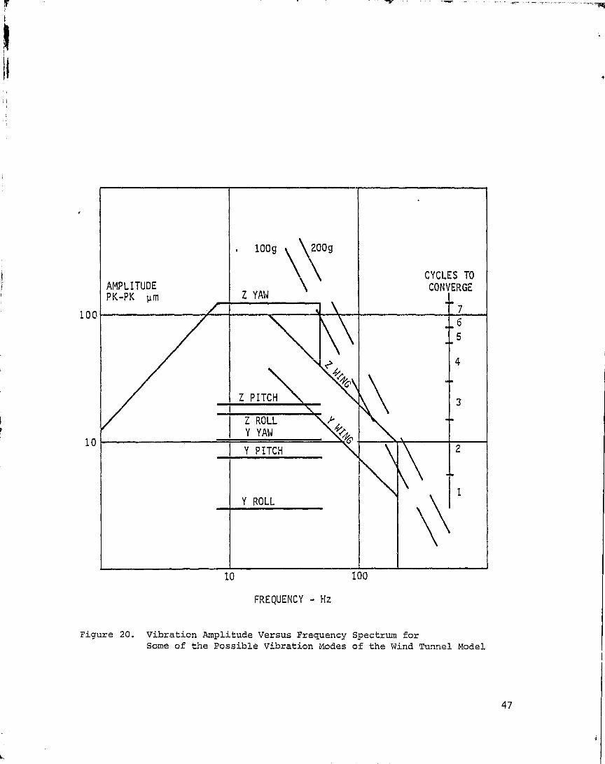
. 100g 200g
CYCLES TO AMPLITUDE CONVERGE PK-PK um Z YAW
76
5
1 4
Z PITCH 3
Z ROLL
Y YAW ^ryc
Y PITCH 2
Y ROLL1
100
10
10 100
FREQUENCY - Hz
Figure 20. Vibration Amplitude Versus Frequency S pectrum forSome of the Possible Vibration Modes of the Wind Tunnel Model
47
I

So far it has its been shown that the vibrational amplitudes arewithin the system capture range, that the measurement is made in a short time,130ps and that the various errors and uncertainties at the faceplate are ofthe order of 0.5 um each.
Several questions still remain. How many targets can the systemhandle, how does the precision depend on this number, how many measurements ofa particular target are made, and what observing strategy should be used.
When sampling a sine wave vibration of frequency f, two timeintervals are important. The first one is t(n) - 130 us (n) + 40 ps (n-1)where n - 1. This is the time used to make a measurement of the vibrationamplitude. While n cycles may be needed to converge to null, it is only thetime involved in making the (last) position measurement that is important. Insampling systems this is called the aperture time. The second time intervalof importance is T (N,n) - Nt(n) + (N) 70 ps. This is the time betweensamples where N targets are scanned and each target requires n cycles forconvergence.
The amplitude response of this sampling process is
(7rft(1) ) (7rfT(N,n) )
A = Ao sin7rft(1) sin 7rfT(N,n)
whereAo is the peak-to-peak vibration amplitude, and
f is the vibration frequency..
The first term, sin ( Vft(1))/vft(1) can be set equal to 1 since for all ampli-tudes and frequencies shown in Figure 20, its value is greater than 0.998.The argument vfT(N,n) can be rewritten in terms of a normalized number oftargets and in a manner showing the dependence upo., vibration frequency andamplitude.
Let
7rfT (No, n) = 7r
fT(Non) = f No(t(n) + 70 ps) = 1
__ 1 1No f (t (n) + 70 us)
__ 1 1f (n(130 us) + (n-1)(40 us) + 70 us)
No is a function of frequency and n, the number of cy^les to converge to null+ 0.5 um. The number of cycles n is, by Figure 18 related to the amplitude ofthe vibration.
48

.
The Figure 21 shows the plot of the normalized amplitude responseof the system versus a normalized number of targets. The normalization factorfor the number of targets is selected based upon the highest vibration fre-quency to be measured. Several values are calculated and listed n the toptable of Figure 21.
If it is necessary to measure a broad vibration spectrum havinglarge amplitudes and high frequencies, the number of targets will berestricted. The top table and graph of Figure 21 show if f - 200 Hz, Ao - 10im and n - 2 cycles to converg°: a system using 5 targets will measure an 8 u mpeak-to-peak amplitude. If the sampling rate and number of targets isselected on the basis of 50 Hz as the maximum frequency, but Ao - 125P m, thesystem will measure 100 u m peak-to-peak and accommodate three targets. Thechief reason for the reduced number of targets is the number of cycles neededto converge. More about that later.
The cases cited have been extreme cases. They permit long termexamination of relatively few targets. It is not always necessary to spendall 2 seconds of the dwell time looking at the same 3 or 5 targets. It isonly necessary that no more than 3 to 5 high frequency or large amplitudetargets be interleaved in the sampling process. At 2700 measurements persecond, each of 5 targets has 54 samples in 0.1 second. The other 1.9 secondscould be devoted to other groups of 5 targets, provided the amplitudes of thelow frequency vibrations, 1-10 Hz, are low. Should there be concern about the1-10 Hz content of the vibrations, consider 10 blocks of 5 targets, each blockof targets is observed for 0.1 secon; a total of 1 second. The 10 blocks arethen examined twice for a 2 second total. The point to be made is that theobserving strategy depends upon the vibration spectrur,t. This aspect meritsfurther examination.
If the system is measuring 50 Hz, 12511 m vibrations at the calcu-lated 820 measurement per second rate, and if there should be a vibration pre-sent whose frequency exceeded 820/2 Hz, the RMS amplitude of this vibrationwill appear as a noise source added to the various other sources. This aspectof the target position sampling is similar to other sampled data systems. Theinput signal must be bandwidth limited or else aliasing of the high frequencycomponents occurs which addes to the in-band noise.
The system presented so far has not been completely optimized.Operating conditions have been representative of fast, general purpose imagedissector cameras. The tracker algorithm is a very simple one. In Section3.5.1 it was mentioned that the error detector curve was non-linear. It isthis non-linearity that costs most of the system speed at large vibrtionamplitudes. The tracker is slow to converge to null; seven samples are neededin the case of 12511m offset.
More light at each target allows the linearization of the errordetector curve by reduction of slope through null. A 2X reduction in thenumber cycles needed to converge various offsets seems possible. The lowerhalf of the Figure 21 table is based on such a 2X reduction.
49
6
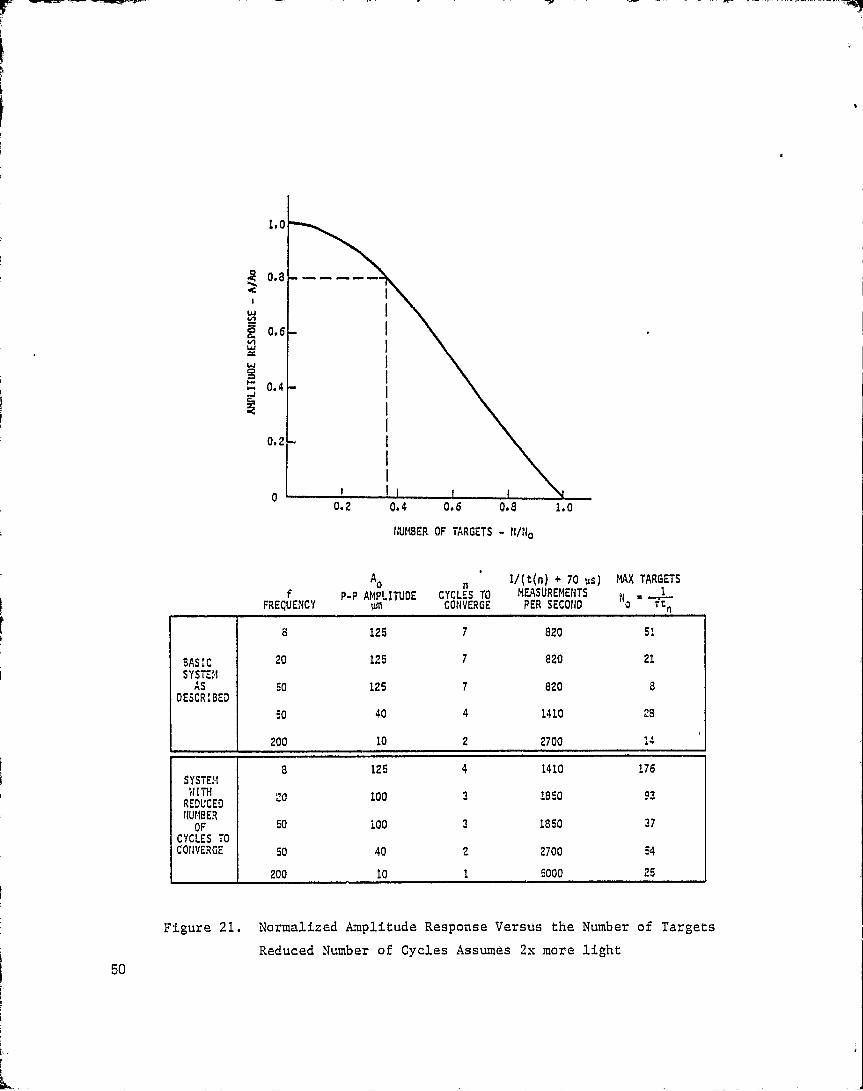
0.2 0.4 0.6 0.8 1.0
NUMBER OF TARGETS - N/Nn
0.8
1.0
0
0.6NWCY
W
V. aJ
K
0.2
A0f P-P AMPLITUDE
FREQUENCY Wn
n 1/(t(n) + 70 us) MAX TARGETS
CYCLES TO MEASUREMENTS N , 1
CONVERGE PER SECOND 0 ftn
8 125 7 820 51
BASIC 20 125 7 820 21
SYSTE'•1AS E 125 7 820 8
DESCRIBED
50 40 4 1410 28
200 10 2 2700 i1
8 125 4 1410 176SYSTEMWITH
'00`
100 3 18 5D 43REDUCEDNUMBEROF 50 i00 3 1850 37
CYCLES TOCONVERGE 50 40 2 2700 54
200 10 1 5000 25
Figure 21. Normalized Amplitude Response Versus the Number of Targets
Reduced Number of Cycles Assumes 2Y more light
50
Ps

7
3.6.3 Camera dynamic motion effects upon system precision. - For asingle camera and small a '"ude vibrations, the changes in apparent targetposition due to camera vibr^_.. cannot be distinguished from changes due tothe vibration of the target.
Consider a target at Point P1. The vector between the image atthe camera and P 1 pivots at the focal point.
Pl
F ba -^
Measurement of P 1 in the presence of small amplitude vibrations'about P 1 is the purpose of the system. (Small, in this case, is in comparisonto the distance between F and P1.)
If the target moves a small distance AP perpendicular to FP 1 , thecorresponding change at the image plane is
Ai =^Pa
where a and b are the magnitudes of I 1 F and FP1.
If the camera moves in a plane perpendicular to I1F by an amountf the focal point F moves. The corresponding Ai change is
Ai + A£ = p f ( a-I-b)`, b f
0i = df -a+b 1 _ A£ b
b (a+b
b b
Of ab
Equal magnitudes of uncorrelated target or camera motion lead tothe same image motion. Therefore target motion plus camera motion must bevector summed and the size of the required capture range determined from thesum.
Magnitudes and frequencies of camera vibrations were unknown atthe time of this study. There will however be vibrations.
3.6.4 Seeing conditions. - The light from a target passes through theair flow in the tunnel, an optical window in the wall of the test section, andthe window on the pressure isolation container for the camera. All threepotentially effect the image quality and the measurement process.
The effects of the windows can be minimized if they are thin flatand not allowed to move relative to the optical axis or camera to model vec-tor. Motions in the plane of the windows have no effect since there is nochange in the optical path length or angles of the rays.
Tilts of the windows can be caused by pressure changes, or tem-perature changes. Tilts of the cameras relative to the window have a similareffect.
51
r

For a ray passing through a 10mm thick quartz window at an angleof 350 to the normal, an angular change of +0.5 degree will cause an apparent±65 ^n shift in target position at the model. The Figure 22 illustrates thispoint. Note that the apparent target shift is proportional to the windowthickness.
The air in the tunnel also acts as an optical element. Eventhough the index of refraction is very close to 1.0, the interface at the win-dow has an effect. The wind tunnel static pressure can change from 1 to 9atmospheres and the temperature from - 1950C to 950C. The index of refractionnt of a gas varies as
n _ __ (no-1) P
t1
(1-0.00366t) 760
where no = 1 . 000298 for nitrogen at 0°C and 76 :j.,:.n Hg.
For the temperature and pressure extremes, the nt value calculatesas
nt (-195 0C, 9atm) = 1.00937
nt (+ 950C, latm) = 1.000221
For rays passing at 35 0 through the 10mm thick window in the testsection wall, the change is 47p m in apparent target position at the model.Again this shift is proportional to window thickness.
There is a variation in this window induced error over the fieldof view since the angle is 35 0 only at the center. The view changes from180 to 520 at the edges of the field of view.
The effects of the temperature and pressure gradients in the vici-nity of the test section window and near the model have not been analyzed.
3.7 Use of Tracker Cameras for TV Viewing of the T,innel Interior
Image dissectors were originally conceived and developed for tele-vision camera tube use. They have been largely replaced by camera tubeshaving image storage (vidicons, etc) because of the greater light efficiencyof frame storage devices.
Image dissectors are mainly used where slow scan is needed; as innarrowband width image transmission systems. The image dissector signalcurrent is independent of the scan rate. The signal current in storage cameratubes is proportional to the scan rate.
For television purposes, the image dissector camera resolution isset by the aperture in the tube. The nominal size being considered for thetracker system is 200pm x 200pm square within a field of view of 10 x 10mmsquare. This results in a TV picture with 100 percent modulation at 50TVL/picture height and zero modulation at 100TVL/picture height; a rather low
52
"I

f^
W/
nt= SIN E) 1 - ---I
(1-SIN 2E)^n2 -niSin20)z
n1 = 1.000298 FOR NITROGEN AT 0°C, 1 ATM
n2 = 1.46 FOR QUARTZ
Figure 22. Refraction at Test Section Window
53
^i
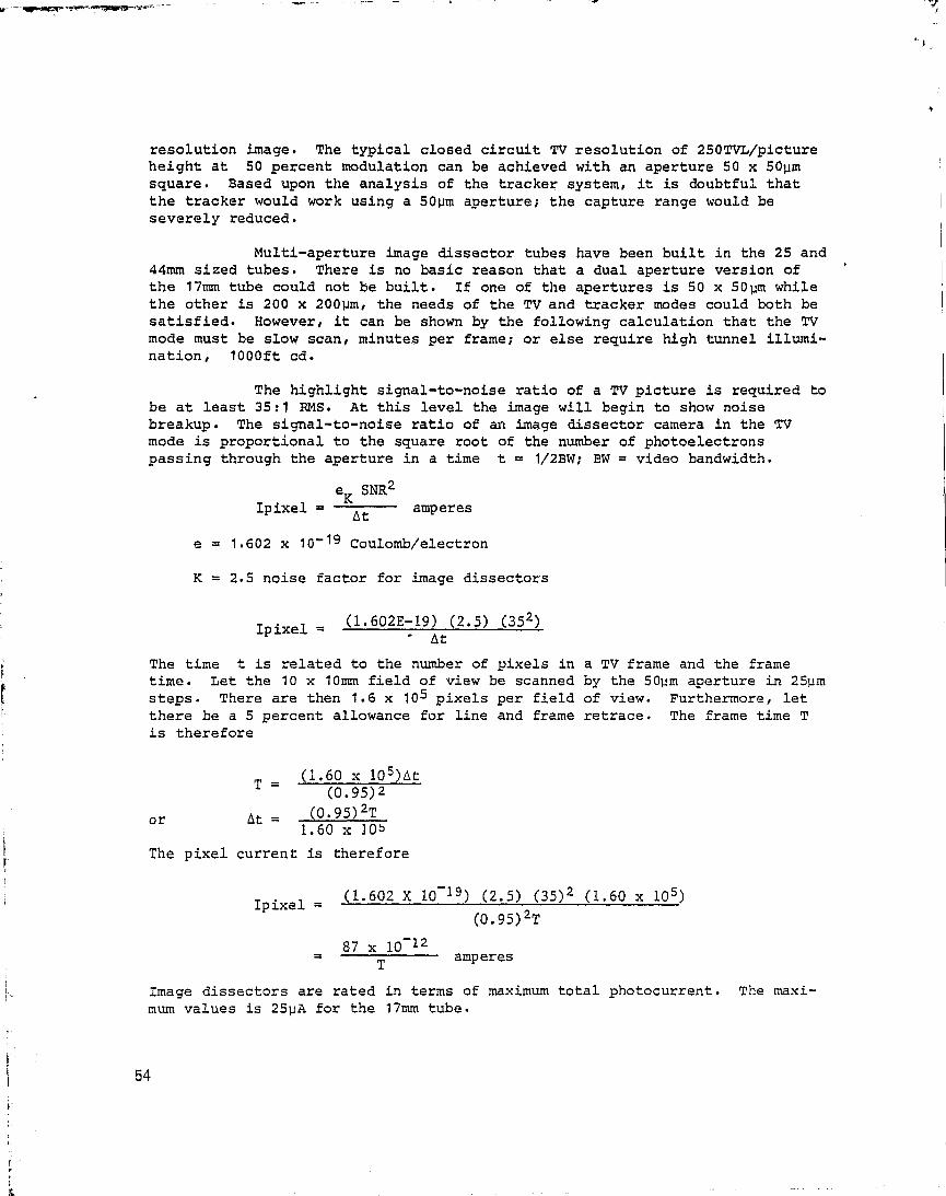
.. N
resolution image. The typical closed circuit TV resolution of 250TVL/pictureheight at 50 percent modulation can be achieved with an aperture 50 x SOUmsquare. Based upon the analysis of the tracker system, it is doubtful thatthe tracker would work using a 50pm aperture; the capture range would beseverely reduced.
Multi-aperture image dissector tubes have been built in the 25 and44mm sized tubes. There is no basic reason that a dual aperture version ofthe 17mm tube could not be built. If one of the apertures is 50 x 50pm whilethe other is 200 x 200um, the needs of the TV and tracker modes could both besatisfied. However, it can be shown by the following calculation that the TVmode must be slow scan, minutes per frame; or else require high tunnel illumi-nation, 1000ft cd.
The highlight signal-to-noise ratio of a TV picture is required tobe at least 35:1 RMS. At this level the image will begin to show noisebreakup. The signal-to-noise ratio of an image dissector camera in the TVmode is proportional to the square root of the number of photoelectronspassing through the aperture in a time t = 1/2BW; BW = video bandwidth.
e SNRZIpixel =
At amperes
e = 1.602 x 10- 19 Coulomb/electron
K = 2.5 noise factor for image dissectors
Ipixel = (1.602E-19) (2.5) (352)At
The time t is related to the number of pixels in a TV frame and the frametime. Let the 10 x 10mm field of view be scanned by the 50pm aperture in 25pmsteps. There are then 1.6 x 10 5 pixels per field of view. Furthermore, letthere be a 5 percent allowance for line and frame retrace. The frame time Tis therefore
T = (1.60 x 10⁵)Ot(0.95)2
or At (0.95)2T1.60 x 105
The pixel current is therefore
Ipixel = (1.602 X 10 -19 ) (2.5) (35) 2 (1.60 x 10⁵)
(0.95)2T
87 x 10-12=
Tamperes
Image dissectors are rated in terms of maximum total photocurrent. The maxi-mum values is 25pA for the 17mm tube.
54
1
4

The total photocurrent is
Ipc = (1.6 x 10 5 ) Ipixel
= .13.9M, < 25 uAT
Therefore, the shortest frame time is about 0.5 second or 2 frames/second.This TV picture will have noticeable flicker for the viewer.
In order to obtain 25VA of photocurrent, the typical 200 A/lumenphotocathode needs a light level of 0.125 lumen or 115 ft cd. This is bright.Scene illumination is 4f# 2 greater or 3600 ft cd for f/2.8.
The conclusion is: use a vidicon.
3.8 Demonstration
A single camera operating under control of a 16-bit mini-computerwas used to demonstrate multi-target ,position measurement and tracking. Thedemonstration showed the ability to search and acquire five targets, to trackthe movement of these five targets while they were moved at a rate and in amanner simulating a change in the angle of attack of a wind tunnel model, andto measure the position of the five targets under conditions simulating thetarget vibrations described in Section 3.3.
Since the demonstration used laboratory equipment, a general pur-pose camera, and a tracker function implemented in software, some scaling ofthe conditions were necessary.
3.8.1 Field of view. - The demonstration field of view was 4 x 4mm com-pared to the desired 10 x 10mm. The smaller field of view was selected inorder to achieve 0.5um deflection increment using the available 13 bit D/Aconverters. Use of a 15 bit converter permits the entire 10 x 10mm field ofview to be utilized at 0.4Um deflection increment.
3.8.2 Targets. - The five point targets were pinhole apertures in ametal plate. The targets were back illuminated by a tungsten light source.The image of the test pattern was demagnified onto the faceplate of the imagedissector camera using a 55mm t/2.8 lens. The background brightness was mini-mized to avoid the added task of writing a background suppression routine inthe target acquisition software. (See Section 3.2.3.)
The test pattern was mounted on a x/y table that permitted it tobe moved about simulating angle of attack changes.
3.8.3 Target acquisition. - A program subroutine caused the camera tobegin raster scan of the field of view in 50um steps. If the video signal wasabove an absolute threshold, the target list was checked for the current coor-dinate or one within a specific range. If no target was listed, the presentone was added. If the target was listed, the scan skipped a safe distancebeyond the target and continued until the raster was completed. The time toacquire the five targets was about 5 seconds.
55
ri

4.0
8.0
i II
4.0
50.8
25.4
Five 25 um Apertures at Locations Indicated
Used with 4:1 Demagnifying Lens
4.0
8.0 17.4REF
DIMENSIONS IN mm
Figure 23. Demonstration Test Pattern
56
ri

3.8.4 Track and measurement. Upon completion of the acquisition, theprogram jumped to the track routine. This routine measured each target posi-tion in sequence, updating the target list. The routine was adaptive. Itwould remain at a target, counting cycles, until the process converged to anoperator specified limit or until five cycles occurred. Upon convergence orfive cycles the routine moved to the next target.
The adaptive ability allowed the tracker to follow very rapidlinear motions of the targets; velocities much greater than would occur duringan angle of attack change. This mode assures that no targets would be lostwhile translating the test pattern rapidly about the field of view.
The tracker action was a time scaled version of the timing diagramshown in Figure 8. Figure 24 shows the comparison between the demonstrationof the tracking algorithm. All software was written in FORTRAN to ease thesoftware development task. There is also a sample called display. This wasused to show, by means of a 'scope in parallel with .;he camera, the convergedestimate of the target position.
Four time scales are involved. They are shown in Table 2. Thefive demonstration targets are scanned in a period equal to about 160 targetsin the design concept system; or 33:1 ratio.
3.8.5 Taraet dvnamic simulation. _ A subroutine was used to generate atable of vibrating target position versus time coordinates. The amplitudesand frequencies used are given in Table 3. The frequencies were scaled topresent the same time scaled motion to the demonstration system as the actualfrequencies would present to a real time system.
The table of vibrating coordinates was then used to disturb thetarget coordinates contained in the target list before the target coordinateswere sent to the tracker. This creates the illusion that the target has movedsince last examined. The tracker then must reconverge to the null position.
Of the conditions listed in Table 3, the tracker occasionallyexperienced difficulty with the third one, the yaw vibration of 126pm x 10umat 50 Hz. Using the 125x rule, this corresponds to 15mm x 1.3mm at the model.It was; not clear if this was a dynamic limit or some unresolved problem withthe demonstration hardware. The 126um is inside the capture range.
Table 2. Comparison of Stereo Electro-Opical Tracker SystemTime Scale with the Demonstration System Time Scale
DemonstrationSystem
Stereo E-0System
Sample Time 200us 201isCycle Time 2600ps 130UsIntercycle Time 29001js 40 s/70us
TOTAL for 3 18.1ms 540uscycles at1 target
57
k'F
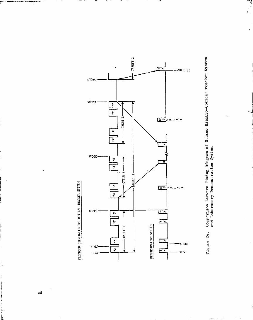
N
lzC7
4N"
srtooss — "
Smolt>
WJUrw
x
W
NNW
w
CF-Jc^a
F-Co,o^
JW
OWCWhNCWOGO
SMOOE5,
• N
W.mot
^ W
w r,C
SitQ£j TI
WJw1+wxI
sr,o L -
t
I
F-
0en
A. xSLU
t,gj
dJ
U
NE-+
cdUvI.0a0
t
a.V) a.eJ a^
P'i
OaJ>aa1ycn
I T U4o Er
u
ro N
En+ x co
OA• 'I.1
to wG ro
•^ 1JH C
Oo ►.uva. ^¢r y A
pq QLr. roO p
..^—^-I T
fA Orl .'^^+ roroaC-+ T r- 10C7
F-NrN
NC I x 4JC SilOQ^^iHH ^
L:II
1
58
r
i

TABLE 3. VIBRATION SIMULATION FREQUENCIES AND AMPLITUDES
EXTREMES ARE
1. PITCH: 13,4uM 50 Hz
3,OuM
2. KOLL: 25,7uM 50 Hz
7,7uM
3, YAW: 125,OuM 50 Hz
10.OuM
4. WIND DYNAMIC: 78,0pm 20 Hz
38.OuM
5. WIND DYNAMIC: 7,8uM 200 Hz
3,8uM
ALL DIMENSIONS ARE PEAK-TO-PEAK AT THE PHOTOCATHODE.
r
rri
59

J
4.0 CONCLUSIONS AND RECOMMENDATIONS
This study and report provides an analytical and experimentalbasis to support the concept of a stereo electro-optical tracker system tomeasure multiple targets attached to aircraft models in the wind tunnel at theNational Transonic Facility. The study showed given 0.em x 1.0m field of viewand 150 Um precision at the model, 5-50 point targets can be acquired andtracked. Furthermore, the intensities of the targets, tunnel background illu-mination, and system data rates are within reasonable bounds. A demonstrationshowed a time scaled simulation of a five target tracker operating at theexpected electro-optical signal-to-noise ratio and desired precision. Theanalysis and demonstration also showed that targets vibrating at frequenciesof 8, 50, and 200 Hz can be located and measured. There is a trade among thenumber of targets per second, the vibration amplitudes, target brightness andcontrast that must be considered.
Several important areas remain to be examined or specified. It isthese areas that introduce an element of risk to the development and use ofthis system concept.
Targets and their attachment to the model are critical to the suc-cess of this concept. This study proposes that LEDs embedded in the model beused. An alternative is fiber optic light pipes, ends polished flush with themodel.
The effects of the distortions in the camera and camera optics onaccuracy needs examination from the viewpoint of the stereo-optic transfor-mation. These distortions can be corrected; but knowledge of the requireddegree of correction for all sources is neededo
The seeing conditions .between the target and the model are impor-tant. Do the shock waves, turbulence and other pressure gratients degrade theaccuracy of the system?
System calibration needs further examination. The study has con-sidered only some of the basic aspects and the general approach.
Lastly, it will be important to know what kind of a thermal andvibrational environment the cameras will experience inside the tunnel pressurevessel. This need is not just for questions of mechanical packaging.Vibrations will contaminate the measurement process. The study shows thesystem can measure vibrating targets on a vibrating model. System speed andnumber of targets depends strongly on the vibration amplitudes and frequen-cies. What are the limits on camera-to-camera and model-to-camera motion.How does the user/experimentor extract useful information about true targetposition from the three dimensional vibrationally perturbed data recorded bythe system.
60
i

4.1 Credits
The writer has found this concept of a stereo electro-opticaltracker system a most facinating one to examine. The help of David Gray ofNASA Langley was most appreciated. He answered many questions about the tun-nel environment and didn't mind repeated requests for vibration data. Thesoftware for the demonstration was written and debugged in about three weekstime by Doug Renselle of SGS, Inc. His contributions greatly aided thedemonstration.
61/(62 blank)
rr

APPENDIX
The Image Dissector as an Optical Tracker
63/(64 blank)
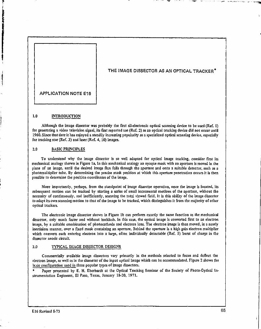
THE IMAGE DISSECTOR AS AN OPTICAL TRACKER`
APPLICATION NOTE E16
1,0 INTRODUCTION
Although the image dissector was probably the first all-electronic optical scanning device to be used (Ref, 1)for generating a video television signal, its first reported use (Ref, 2) as an optical tracking device did not occur until1960. Since that date it has enjoyed a steadily increasing popularity as a specialized optical scanning device, especiallyfor tracking star (Ref, 3) and laser (Ref. 4, 10) images.
2.0 BASIC PRINCIPLES
To understand why the image dissector is so well adapted for optical image tracking, consider first itsmechanical analogy shown in Figure la. In this mechanical analogy an opaque mask with an aperture is moved in theplane of an Image, until the desired image flux falls through the aperture and onto a suitable detector, such as aphotomultiplier tube. By determining the precise mask position at which this aperture penetration occurs it is thenpossible to determine the position coordinates of the image.
More importantly, perhaps, from the standpoint of image dissector operation, once the image is located, itssubsequent motion can be tracked by starting a series of small incremental motions of the aperture, without thenecessity of continuously, and inefficiently, scanning the total viewed field. It is this ability of the image dissectorto adapt its own scanning motion to that of the image to be tracked, which distinguishes it from the majority of otheroptical trackers.
The electronic image dissector shown in Figure lb can perform exactly the same function as the mechanicaldissector, only much faster and without backlash. In this case, the optical image is converted first to an electronimage, by a suitable combination of photocathode and electron lens. The electron image is then moved, in a nearlyinertialess manner, over a fixed mask containing an aperture. Behind the aperture is a high gain electron multiplierwhich converts each entering electron into a large, often individually detectable (Ref, 5) burst of charge in thedissector anode circuit,
3,0 TYPICAL WAGE DISSECTOR DESIGNS
Commercially available image dissectors vary primarily in the methods selected to focus and deflect theelectron image, as well as in the diameter of the input uptical image which can be accommodated, Figure 2 shows thebasic configuration used in three popular types of image dissectors.
* Paper presented by E. H. Eberhardt at the Optical Tracking Seminar of the Society of Photo-Optical In-strumentation Engineers, El Paso, Texas, January 18-20, 1971,
E16 Revised 8 .73 65

COOL? Ira#.
.fa tiara/
tr#rINMNI (HrtwrNr /,r
•I : '^"``
TTy[^rF ^r^^r ^ 1 11111)O
RD4 PRODUOIBT.I'Try,^„#.r^, ^."
- . -9 4 /l%^^ f,r..Nlw/PAC',;,
, IS POORt ORIGAIJO,rHI
s«t^
OIJIfI O/IIN Wy.r1 I/ IIINw.,e ♦ ^
OY'If#.wIf IM!MU./`w II/iOlI/ItfNwr
4
001 M#f•f,rtfl =If b,,Itlle
1rif"00 /w#/IwM I I.of ;...b 111/fl.we Mlf. (F.
'flw.40- `W {r ! (llfflwYrrl /uN
^^^.+.^ ^ ^• I f ar ^,-
♦ F. 1#'•'^ {•tl/r+fll .ter,. 3^^; ^ '^^• 4r/,:
^..^ /•Ihtlam...• (1111/,_..
..^•
j ;
N#INI/MN rn^j rr.1/I (4111few INId1IJIrl/M
/t,
YIrH II#tllr I/IIIr wlI /Ir M#:.r/I ~ Mr.try #Jtf#/
tf1 rr ,r I^q T ^111tt 1 9f /Mfnaf/Illrwe/o(f1 C/.—he, Of 0"' W JowmffOwarsA/
Fitwf It MECHANICAL ANO ELECTRONIC IMAGE OISSECTORS
m",
OlrrHtr/ f.M
JHrn r/` qur.qI
Ift.
tra
fi.# VII#4WIP 1#000
OIINtr/w (470
^`^ 0 Jt#n/InI.f.Or./
MNHI.MII %g (^IfNw
X8888 V.II,r,Ir
w MI..q Hrtt 1-411 0411tUr, u1. 0 g01 tied. 'np iNe r 4 t 1r11J914.e41 ?4010, 140u. f4c1J. 14011 It?.
ON;HIIw (Hq(/afrl/NII? fHH (JI wo,^` d (rift
^^^CQ^^
(ItfrlrVrl/rI/Jrr
'.. 11 ,11111 •nt11 01.10041 St., "Oil,$ 111.;tle r.Nts f-4, 1 #/11, r*'-10. 1. 1* 1.143 04704 r It'
CrrNlllrfLt fell$ ("411001\\ ( rl ry $ llb t W1 0f , #. /yr1l t Jr1ve
Nayaaf#. f#tlprli 1 .
f slowVrrr #' rr
/III/
^^ llle u*... t00Yf - ^^^ C rrI-.. .ION• ___._... _._....
. I II^l I
(n.Hrr. it.•^ • l09.^ ,yurN1
i OH.rrN i
1 r
I ' r
r
..Jf
^, ^... rp. N" Orr/brLal
IVI OrrH.rr^N OrfIIIIIIwOIIII.f1.
it1Ifr.rnrn./u rU x .11. P'S'W#f. .rr4 ON.../.IIIti ,$Hl.t O.r4tein f l 4101 'OfBi
F.p.re 2. TYPES CF MADE CISSECTORS
F,gwi Y OCCULTAT ION CHARACTERISTICS
E16 Revised 8-73
t
i
f
66Ii
iI.

.,a
At the top, Figure 2a, is a Vidissector® (Fcotnote 1), image dissector, an advanced version of the earliest,
magnetically focused and deflected dissectors. A fine pre-acceleration mesh is used in close proximity to the photo-
cathode, to accelerate the photoelectrons up to their full velocity as quickly as possible, followed by an electric-field-
free drift and deflection space prior to the defining aperture plate. This tube is designed to operate satisfactorily in the
same type of magnetic focus and deflection Boils used for vidicons and image orthicons, Such an image dissector was
used as a star tracker in the first X-15 experimental aircraft (Ref. 6). Its properties as a star tracker have been
described by Ostroff and Romanczyk (Ref. 7);
In Figure 2b is shown the basic configuration of a hybrid image dissector with electrostatic focusing and
magnetic deflection. This type of dissector, often called a "star tracker" tube, was used in the fast reported dis-
sector tracker (Ref. 2) and in other, more recent trackers (Ref. 8, 9, 10), including the star trackers used in Aerobee
rockets and on the Lunar Orbiter spacecraft (Ref. 3).
In Figure 2c is shown the basic configuration of a Reconotron all-electrostatic image dissector which was used
as an azimuth star tracker on the ,Mariner series of spacecraft (Ref. 11).
4.0 PERFORMANCE CHARACTERISTICS OF IMAGE DISSECTORS
4.1 Rise (or Occultation) Distance
When a small, "point-source" optical image is focussed onto an image dissector, as indicated in Figure 3, and a
linear deflection signal is applied, the aperture can be made to move (Footnote 2) across this point source image,
generating a pedestal-like output signal. Ideally this signal should have a sharp rise and decay characteristic, as in-
dicated by the dashed lines in Figure 3 as the aperture occults the point source image. In practice, the rise and decay
characteristics are somewhat rounded, with the degree of rounding conveniently describing the capabilities of a
particular image dissector. Quantitatively, the rounding can be measured in terms of the aperture displacement, w,
measured at the photocathode, necessary to change the output signal between the 107o and 9011'o response points, as
indicated. The magnitude of the resulting rise distance, or occultation distance, w, is an important operational
characteristic of an image dissector.
Figure 4 shows how a finite rise distance is generated internally within an image dissector. The group of
photoelectrons emitted from a point image on the photocathode, exit from the photocathode with a finite spread of
energies (commonly averaging about 0.5 eV) and directed at various angles (commonly with an approximately
Lambertian distribution). Thus these photoelectrons tend to spread out as they leave the photocathode, progressively
destroying the image quality. This tendency to spread is counteracted by the focussing action of the electron lens
which brings the bundle of emitted electrons back to a near-point-source size at its focal plane. It can be shown that
the width-at-half-maximum of the resulting, approximately Gaussian, beam density distribution at the image plane is
approximately equal to the M-901c rise distance, w. Thus, there are four essentially synonomous terms for the
parameter, w, at focus, namely:
w = beam width = beam diameter = rise distance = occultation distance
Figure 5 shows what the total electron beam profile actually looks like in Vidissector image dissectors, for a
point source input, and three possible magnetic focus conditions, namely: one loop, two loops and three loops of
focus. Focus at the aperture can be assured by choosing a combination of the solenoidal magnetic field strength,
1: Trademark, International Telephone & Telegraph Corp.
2: Although the electron image actually scans over a fixed aperture in the image dissector, it is often helpful in
describing dissector behavior to talk in terms of the mechanical analogy, where the aperture is moved over the
optical image.
E16 Revised 8.73E7

Curran/ 0«1,4' C«reMaarpDomeudorr OetuNena"'^ haul feetwo/a or f#Cal Prbae
OI«e[I«qhCIPanl JArase{ fne/sCelnoee Fwdfeel
A% 100%' 0 50% 10 0% 0I 90%
•' ^ i j i ^ l
ePon ; /' = , T RDPRODUCTI3IT /I7'Y OF `I~xll;
^^"o ` full I10•^0% ORIGINAL PAGI IT IS Po olt4o«ry%e wra/n ePMae I a/ Noll puau/
mew.Ymr ur
n I Occullaloo po/uxe full wra/n a/ Mel/ Ala.rrnum n /Jne O/o/aaea
Flpu/o 41 RELATION BETWEEN THE POINT SPREAD FUNCTION OF THEELECTRON BEAM AND THE RISE DISTANCE, r,
Vim,I PnalaoomoaePna/ocalnoae (OV)fine MC20 (4 V )
aMlrr/O./II
JII.
A wI«oP/ere
^ Vlrllll/
JI11e
n•I
LILI2
01/2
n•21 ^
2V I L+L. J01/S
jI ^
IB
j n s S
1 ,
^L a SD I LL±L.
^-- 1 r
Figure SI BE'M LOOP SHAPES IN V1015SECTOR IMAGE D15SECTORS(SHOWING
1
FIRST THREE LOOPS" OF FOCUS) \L
8, 3 2-r. ; 2. V ^Y D• = 0.S3 L BLS ^^=1 J
3
l.L. e V
W = 1,23 L. ^V" V'jf Ion e/2 = 0.83 I ^.JT
I^
JYloul s. I•NlJ/N C/+rnrn
D•r11 I r
100 ^' i 1U oYlnr J
IJ/N OrnrallO M-"./II/J/
_— - —^ - - --^ IY+Olrwrl/.....+I/CIM.NwI, jlarllrl/1/ I/
SIN Oirhrl. rrl
Fiyule H TYPICAL ROSETTE-SCAN STAR TRACKER MODE
68 E16 Revised 8-73

Bn in webers/meter 2 ; the photocathode-to-mesh voltage, V, in volts; the photocathode-to-aperture spacing, L, in
meters; the photocathode-to-mesh spacing, Lm, in meters; and the charge to mass radio, a/m, of the electron, in
coulombs/kg, such that the following equation is satisfied:
_ 2 7r 7? 2 mV 1/2Bn
L+Lm a (1)
Insofar as both the electric and magnetic fields are uniform, and the aberrations introduced by the non-
uniform deflection fields can be ignored, the beam width, w, at focus is given by:
(Vro Vzo) 1/2W Z! 1.23 L m V (2)
where Vro is the average radial emission energy component of the photoelectrons, and Vz O is the average axial
component, in electron volts.
For a typical Vidissector image dissector, such as an F4052, with L = 22.5 cm, Lm = 0.32 cm, V =600 volts
and 2 Vro ' Vzo ^ 0.3 eV (white light input to a muitialkali photocathode), Equation 2 yields a value of 1.4
micrometers for the beam width, w. This is approximately 0.003% of the total image field diameter which can be
scanned in such a tube (4.2 cm), illustrating the excellent limiting "resolution" characteristics which can be
achieved. ;Measured rise distances as short at 2-5 micrometers, have actually been observed in an F4052 image
dissector camera.
The maximum (off focus) beam diameter, D n , and the beam convergence angle,6 (useful in estimating depth
of focus) are given in Vidissector image dissectors by:
nDn = 0 .53 (L + Lm) (Vro/V) 1/2
(3)
tan (0/2) = 0.83 (V ro/V) 1/2
(4)
4,2 Possible Tracking Modes
One type of simplified "rosette" scan which can be used (Ref. 2, 3) for tracking a star or laser image with a dis-sector is shown in Figure 6. Here one applies successively, a small positive horizontal aperture displacement andreturn, a small positive vertical aperture displace and return, etc., as shown, with the star image initially known to belocated somewhere within the aperture area. If the star image is centered within the rest position of the aperture, theoutput signal, as illustrated, will be a uniform symmetrical series of pulses, of rise distance, w.
On the other hand, if the star is displaced, the output pulses will become assymmetrical in width, generating afundamental component of the scan "frequency", fo , whose amplitude is linearly proportional to the offset dis-placement of the image, and whose phase determines the direction of the displacement (see Figure 6). This type ofsimple, but efficient star tracker, combined with mechanical gimballing to keep the stellar image within the viewedaperture area has been used (Ref. 3) to track stars within less than 1 micrometer displacement accuracy at thephotocathode. For a particular optical system used, th ,,s was equivalent to better than 10 arc seconds tracking ac-curacy, Note that the tracking information, to a first approximation is independent of the magnitude of the risedistance, w, and of the magnitude of the stellar flux, F, (assuming that the magnitude of the fo frequency componentis referenced to the magnitude of the 2fo component). If so desired, the electronically generated image offset in-formation can be converted to a "DC" centering deflection displacement of the aperture. The aperture can then bemade to electronically follow the motion of the star image within the field of view.
E16 Revised F-73
69
4

Four other possible tracking scan modes are shown in Figure 7. The first, Figure 7a, illustrates the azimuth-only type of tracker used in the Mariner spacecraft (Ref. 11). This tracking mode takes advantage of the fact that along narrow, slit-shaped aperture can be built into the image dissector tube, with line scan permitting azimuthposition information to be extracted without regard to the elevation of the star image.
Figure 7b is a similar tracker, using an L-shaped aperture. Here, both azimuth and elevation information for astar image (or images) can be generated by use of a corresponding L-shaped scan.
Figure 7c illustrates a somewhat more complex type of image dissector tracker. In this case a small apertureis rotated, or wobbled, with a small amplitude, such that image irradiance gradient information is generated. Thecenter of the scan can then be made to move electronically at right angles to this gradient. The dissector then auto-matically traces out equal irradiance level contours. Such a scheme has been used in an eyeball tracker (Ref. 12) fortracking the pupil of the eye.
And finally, a rather sophisticated image dissector tracker can be constructed whose internal aperture can beadjusted electronically to a specific shape, such as the letter, "A", illustrated in Figure 6d, When such a custom-shaped aperture is then scanned over an image field, it will generate a large, sharply defined, `correlation spike"whenever it crosses precisely over an image area of the same shape. This sharp correlation spike can be used (Ref. 13,14) with great effectiveness to track complex image shapes against a non-uniform background.
If so desired, dissector tubes may be supplied with multiple apertures, each with its separate read-out electronmultiplier, for special optical tracking applications (Ref. 15).
4.3 Signal-to-Noise Ratio
Usually, only one type of random noise is encountered in image dissector trackers, namely the inherentstatistical fluctuations of the photoelectrons emitted from the photocathode. Dark noise, i.e., random residualnoise generated by the tube itself, and by the external amplifier circuits, in the absence of input flux, is nearlyalways negligible. This is a direct benefit of the large (> 10 5), nearly-noise-free charge amplification present in theelectron multiplier of the image dissector.
To calculate the expected magnitude of the photoelectron noise and show how it limits the ability to findand track images, it is convenient, and especially instructive of image dissector behavior, to assume that the dissectorscans by making a series of discrete image intensity samples. In this sampling process, illustrated in Figure 8, the scanstops on each aperture-sized element for a short time, A t, called the dwell time. It can then make a "count"(Footnote 3) of the total number of photoelectrons collected by the aperture.
When only a uniform background irradiance is incident on the photocathode, the resultant output count, nbwill be given by
nb = L a Sb E A t (5)
3: While the image dissector can actually count individual output anode pulses corresponding to individual photo-electrons entering the aperture, it is more usual in practice to accumulate these anode charge pulses and generate anaverage output current.
70
E16 Revised 8-73
rr
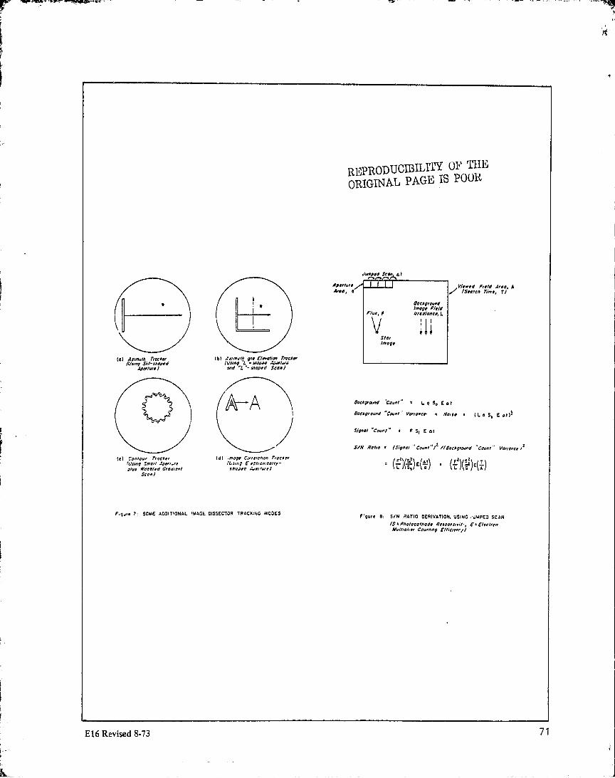
/pblurlArm, a
Field Arro, A
I rlmr, TI
Flue, F
VS/or/moor
BoetprowdImopt Fieldlrrolinner, L
t^W
1
t
ORIGINAL PPAGL1 S PUILL0
laI fu. 0/$1llyinod d
//,
dprrlurr
l
l
p^q.,,
let Conrour rrortel'unnp Smoe .Jprn.rr
plus w000lyd 6/odUnlSemi/
101 ANmul? 9.df/~t" revere.furinp L vwopedoad I "-ttdped Won;
161 ;mogr cx'venan rwcoer/('3W E:rdiomeollr-tnupre -ver/wel
8009'0 rd 'Count" s L o Sr E AtBoNprowd "CeVnl Vononer c Noire . I L a 5, E A10
Sipnol "Count" r F S 1 E At
SIN Noho r tSipnol "Count"/ 2 /tsaroq'ound "Count' Vononor/=
L JAS,/ E t of/ r (L /(5 /E\A
F,qurr T: SOME ACOITIONAL IMAOL DISSECTOR TRACXING MODES Flqurr 17: S/N RATIO DERIVATION, USING.'JMPED SCANt5+Pnotorolnode Feroanl—h ' "-C/retronMul/lol/rr, Count/ng £!/ielme^/
E16 Revised 8-73
71
1
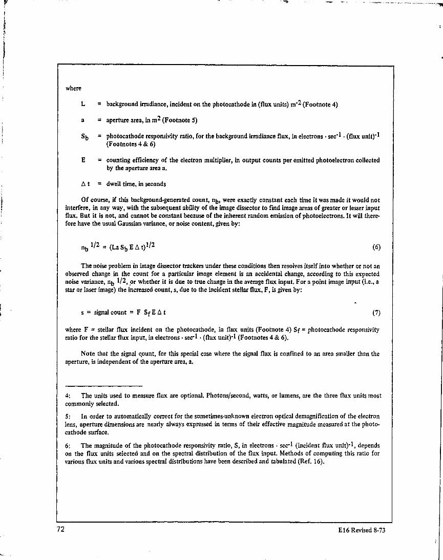
where
L = background irradiance, incident on the photocathode in (flux units) m-2 (Footnote 4)
= aperture area, in m2 (Footnote 5)
Sb = photocathode responsivity ratio, for the background irradiance flux, in electrons - sec- I - (flux unit)'1(Footnotes 4 & 6)
E
= counting efficiency of the electron multiplier, in output counts per emitted photoelectron collected
by the aperture area a.
0 t = dwell time, in seconds
Of course, if this background-generated count, n b, were exactly constant each time it was made it would not
interfere, in any way, with the subsequent ability of the image dissector to find image areas of greater or lesser input
flux. But it is not, and cannot be constant because of the inherent random emission of photoelectrons. It will there-
fore have the usual Gaussian variance, or noise content, given by;
nb 1/2 = (La S E At) 1 /2 (6)
The noise problem in image dissector trackers under these conditions then resolves itself into whether or not an
observed change in the count for a particular image element is an accidental change, according to this expected
noise variance, nb 1 /2 , or whether it is due to true change in the average flux input. For a point image input (i.e., a
star or laser image) the increased count, s, due to the incident stellar flux, F, is given by:
s = signal count = F Sf E A t (7)
where F = stellar flux incident on the photocathode, in flux units (Footnote 4) Sf = photocathode responsivity
ratio for the stellar flux input, in electrons - sec- 1 - (flux unit),I (Footnotes 4 & 6).
Note that the signal count, for this special case where the signal flux is confined to an area smaller than the
aperture, is independent of the aperture area, a.
4: The units used to measure flux are optional. Photons/second, watts, or lumens, are the three flux units most
commonly selected.
5: In order to automatically correct for the sometimes-unknown electron optical demagnification of the electron
lens, aperture dimensions are nearly always expressed in terms of their effective magnitude measured at the photo-
cathode surface.
6: The magnitude of the photocathode responsivity ratio, S, in electrons • sec-1 (incident flux unit)- I , depends
on the flux units selected and on the spectral distribution of the flux input. Methods of computing this ratio for
various flux units and various spectral distributions have been described and tabulated (Ref. 16).
72 E16 Revised 8-73

An effective signal-to-noise output power (Footnote 7) radio SNPRtrack for image dissector star trackers cantherefore be written down directly as:
F2Sf'—E2^t2
SNPRtrack
= (F2/L) (Sf--/Sb) E (At/a) (8)
LaSbEAt
The importance of maintaining high stellar flux, F, high cathode responsivity to this stellar flux, Sf, and high
electron multiplier counting efficiency, E, is evident from this equation.
However, changes in the dwell time A t, and aperture area, a, must be interpreted with care, since there is
usually an interdependence between the aperture area, a, and the dwell time A t. This can be illustrated for the
special case where a square aperture image dissector scans a total field area, A, in a total search time, T, with no
scan overlap and negligible fly back time. In this special case the ratio,At/a equals T/A, and the signal-to-noise ratio
becomes:
SNPRtrack ° (F2/L) (Sf 2/Sb) E (T/A) (8a)
In this alternative form, and for this scan pattern, it can be seen that the signal-to-noise ratio is independent of
the Celected aperture area. Thus in certain star tracking modes one is free to choose any desired aperture size, and
thus to locate the star image as precisely as needed, without loss of signal-to-noise ratio.
This rather surprising deduction does not hold when the star image becomes comparable to the aperture size,
or when the sigvmi is derived from changes in the input fleet density level, as in TV-type scanning, where the signal is
linearly proportional to aperture area, a. For these latter situations, the more conventional signal-to-noise ratio re-
lationships (Ref. 17) will apply.
If a current measuring external circuit with a noise bandwidth, Af, is used instead of a counting circuit, the
dwell time, AT, is usually replaced by:
At = (2 A 0-1 (9)
and the counting efficiency, E, by:
E = k- 1(10)
where k is the noise factor (Ref. 18) of the electron multiplier. Counting efficiencies of 0.85 to 0.95 output counts
per emitted photoelectron are easily achieved in image dissectors with well-designed first dynode geometry (Ref. 5).
This is reduced by the electron transmission ratio of the mesh (typically 0.6 to 0.65) if a mesh is used, as in Vidissector
image dissectors, between the photocathode and the first dynode.
7: Image dissector signal-to-noise ratios are also often written in terms of the ratio of output signal current to
output noise current.
E16 Revised 8-73
73
i__ —

5.0 ADVANTAGES, DISADVANTAGES, AND PROBLEMS OF IMAGE DISSECTORS
The optical tracking systems designer, faced with the problem of selecting an appropriate tracking method,needs to know both the advantages and the disadvantages of the image dissector, as well as some of the problemswhich can arise. Unfortunately most of the important problem areas concern specific tube types, and often specifictube samples, so it is difficult to make generalized conclusions. Nevertheless some useful statements can be made.
5.1 Advantages of Image Dissectors
5.1.1 Fast Deflection: The low inertia of electrons allows fast deflection. Limits are more often established bythe external deflection circuits, 1 fl sec jump times between adjacent image elements and 100 k sec jump timesacross a full image diameter have been achieved, and improvements are in progress.
5.1.2 Adaptable Scan: The image dissector can easily be switched on command, from one scan mode toanother, e.g. from search scan to track scan or from search scan to contour-tracing scan, or from jumped scan tocontinuous scan.
5.1.3 High Tracking Mode Sensitivity: When the aperture pf an image dissector is actually observing an opticalimage to be tracked, it enjoys very high effective sensitivity, equal to or better than the best photomultiplier tubes.No difficulty is experienced in counting individual photoelectrons, and the spurious dark count encountered is ex-tremely small (typically a few counts/second or less),
5.1.4 Linear Input-Output: The output from an image dissector is linearly proportional to the input fluxovermany orders of magnitude. Thus the image dissector can be used as a precision microphotometer simultaneouslywith scan tracking (Ref. 19). This property is also often useful in deriving optical intensity information for a com-puter input (Ref. 20).
5.1.5 Wide Bandwidth: The image dissector can follow intensity modulation of the input flux seen by theaperture from DC up to many megahertz. With special electron multipliers this can be extended into the gigahertzregion, making the image dissector especially attractive as a dual mode sensor for optical tracking and wide band-width optical communications systems (Ref, 4, 28).
5.1.6 No Gear or Rearing Backlash: Since the aperture as well as the deflection and components can be per-manently attached to the tube envelope, there are minimal opportunities for boresight offset errors to occur.
5.1.7 Rugged Construction: The inherent simplicity of image dissector construction permits the tubes to beruggedized. No difficulty has been experienced in meeting the mechanical requirements for rocket and missilelaunch; in fact at least one image dissector tracker tube has survived an Aerobee rocket crash landing and was sub-sequently re-used.
5.1.8 Long Life: Dissectors have now been in essentially continuous service for over 30 years. The absence of ashort-lived thermionic cathode, used in other TV camera tubes, make this performance possible.
5.1.9 Damage Resistance: The dissector is inherently resistent (Ref. 21) to many types of damage such asmomentary flux input overloading, nuclear radiation exposure, accidental over-voltaging, etc. For example, aVidissector image dissector in the ATS-F spin stabilized satellite (Ref. 22), has withstood periodic direct solar ex-posure through a high speed optical system, with no sun-shuttering and with no removal of voltages, for over threeyears in space without measurable degradation.
5.1.10 Fast Turn-On: An image dissector is ready to go within a few milliseconds, at most, after application ofthe proper operating potentials.
74 E16 Revised 8-73
S.1.11 Wide Spectral Response: Photocathodes for Image dissectors cart be formed with spectral responses
ranging from the far ultraviolet region, to the near infrared (I10 nm to 1200 run),
5.2 Disadvantages and Problem Areas^^^ ! Mt wee►
5.2.1 Low Search-Mode Sensitivity: Since the image dissector wastes altimage photoelectron information
which does not happen to pass through Its aperture at any instant of time, it is Inherently less sensitive than "storage"
type scanning tubes such as the image orthicon and vidicon, for the wide field search mode, where a large number of
image elements must be searched before the image to be tracked is located.
5.2.2 Non-uniform Response (Shading, Blemishes, etc.): The input-output responsivity of an image dissector
will generally vary, at least by a small amount, from one point to another over the viewed field. If the change iz
gradual, it is called "shading", with variations within + 10% or so over the image field being typical. More serious, in
many applications, are the rather sharp variations called blemishes which can occur within one or more picture ele-
ments. The number and amplitude of these blemishes is often an individual tube-sample characteristic. However, as
in other TV camera tubes, blemish numbers can be kept small by proper quality control during tube manufacture.
5.2.3 Off-Axis Defocussing: When a peripheral image element is deflected into the aperture of a dissector, the
effective aperture size and shape, and the rise distance, w, may change. This can be, and commonly is correctable in
practice by applying a dynamic focus signal to the tube focus circuits in synchronism with the deflection. Such
dynamic focus signals are usually easy to apply. The residual defocussing, after correction, is partially limited by
tube design and partially by the external focus and deflection coil design. In Vidissector image dissectors, with cus-
tom wound coils, residual rise distances as low as 3-5 Lt m after dynamic focusing, have beer- achieved over the full
usable input image area.
5.2.4 Off-Axis Distortion: The actual deflection produced by applying a deflection signal is not necessarily
identically proportional to the deflection signal. The resulting image distortion is especially serious in electro-
statically focused tubes, which are really satisfactory only for near-axis tracking. In magnetically focused Vidissector
tubes the image distortion is largely a function of the coil design geometry, with aperture displacements within less
than 1 17o of their linearly predicted position being readily achieved.
5.2.5 Boresight Hysteresis: Although the image dissector has no gear and bearing backlash problems, therecan be an equivalent problem introduced by hysteresis in the deflection circuits (failure to reproduce exactly thesame aperture position for a given applied deflection signal). In magnetically focused tubes this can be caused bymagnetic hysteresis in the magnetic core material or magnetic shielding material. In electrostatically focused tubes itcan be caused by electrostatic charging of internal insulator surfaces. With proper tube and coil design these effectscan often be reduced to negligible values.
5.2.6 Scan Delay: There can be a finite delay between the time a deflection signal is applied and the time theaperture reaches its new position. This can be due to eddy current losses occurring in the metal parts in magneticallydeflected tubes, or to finite insulator charging time in electrostatically deflected tubes. This problem can beespecially troublesome in random jumped scanning (not usually encountered in optical trackers) in which theaperture must move very rapidly over large distances and then be suddenly stopped.
5.2.7 Photocathode Fatigue: With continuous intensive current density loading of a photocathode, it ispossible to gradually reduce its responsh ity, especially in the red region of the spectrum. By proper tube design, thisphotocathode fatigue can be greatly reduced, with total photocathode emission charge densities ranging up toseveral cotilombs/cm2. Barring tube breakage, sudden, catastrophic failure is almost never encountered.
E16 Revised 8-73 75

5.2.8 Gain Stability: The high gain properties of electron multipliers make them inherently sensitive to themagnitude of the applied voltage and to small chemical and physical changes In the dynode surfaces. Thus theapplied voltage should be regulated, and the temperature held within reasonable limits, such as + IO aC, to achievestable gain.
6.0 SUMMARY
It can be seen that the image dissector is nearly an ideal device for certain optical tracking applications. It can,and does, compete with mechanical trackers in some areas, and in other areas, with more conventionalraster-scan-only television camera tubes.
76 E16 Revised 8-73

REFERENCES
1,
Farnsworth, P.T., J, FraiWin Inst. 218, 411 (1934).
2. Atwill, W„ Electronics 23, 88 (July, 1960).
3. Dieters, R.A., Eisenhut, D,R., and Gates, R.F,, Electrical Communication 42, 204 (1967).
4. Dixon, T.P., Wyman, C.L., and Coombes, H.D,, Navigation 13, 231 (1966).
5. Eberhardt, E.H., Applied Optics 6, 161, (1967).
6. McGarty,T.P. and Nardella, P.C. (M.I.T. Instrumentation Laboratory), Private Communication (1968),
7,
Ostroff, A.J., and Romanczyk, K.C„ NASA Technical Note TN•D-5281 (June, 1969).
8. Fitzgerald, BY,, J. SMPTE 78, 29 (1969).
9. Product Engineering, p. 40 (December 21, 1970).
10,
Lucy, R.F., Peters, C.J., McGann, E.J., and Lang, K.T„ Applied Optics 5, 517 (1966).
11. Goss, W,C., Applied Optics 9, 1056 (1970).
12. Merchant, J., Space Aeronautics, p. 92 (February, 1968).
13. Pennie, E., Wright-Patterson Air Force Base Technical Report TR-68-9, (1968).
14. Hawkins, J.K., and Elerding, G.J., Proc. SPIE Computerized Imaging Techniques Seminar, p. VI-1
(June, 1967).
15. Nielsen, R.S., and Ford, MA., Optical and Electro-Optical Information Processing, Chapt. 26
(M.1.T. Press, 1965).
16. Eberhardt, E.H., Applied Optics 7, 1037 (1968),
17. ITT Reference Data for Radio Engineers, p. 410 (4eh Edition, Stratford Press, 1956).
18. Eberhardt, E.H., Applied Optics 6, 359 (1967).
19. Ball, W.F., and Hoag, A.A., Sky and Telescope, p. 22 (January, 1968),
20. Win„ M.E., Electro-Optical Systems Design, p. 54 (Nov./Dec., 1969).
21. Wolff, C., Applied Optics 5, 1838 (1966).
22. Branchflower, GA., Foote, R.H., and Figgins, D., IEEE Trans. on Aerospace and Electronic Systems.
Supplement AES-3, 63 (November 1967).
23, Lucy, R.F., Proc. IEEE 51. 1962 (1963).
E16 Revised 8-73
77/(78 blank)