This article is downloaded from

http://researchoutput.csu.edu.au It is the paper published as

Author: J. Gao, P. Kwan and X. Huang

Title: Comprehensive Analysis for the Local Fisher Discriminant Analysis

Journal: International Journal of Pattern Recognition and Artificial Intelligence

ISSN: 0218-0014 1793-6381

Year: 2009

Volume: 23

Issue: 6

Pages: 1129-1143

Abstract: Using data local information, the recently proposed local Fisher Discriminant Analysis (LFDA) algorithm (Sugiyama, 2007) provides a new way of handling the multimodal issues within classes where the conventional Fisher Discriminant Analysis(FDA) algorithm fails. Like the FDA algorithm -€” its global counterpart FDA algorithm, the LFDA suffers when it is applied to the higher dimensional data sets.In this paper we propose a new formulation by which a robust algorithm can beformed. The new algorithm offers more robust results for higher dimensional datasets when compared with the LFDA in most cases. By extensive simulation studies,we have demonstrated the practical usefulness and robustness of our new algorithmin data visualization.

Author Address: xhuang@csu.edu.au

URL: http://dx.doi.org/10.1142/S0218001409007478

http://journals.wspc.com.sg/ijprai/ijprai.shtml

http://researchoutput.csu.edu.au/R/-?func=dbin-jump-full&object_id=12402&local_base=GEN01-CSU01

http://unilinc20.unilinc.edu.au:80/F/?func=direct&doc_number=001483947&local_base=L25XX

CRO Number: 12402

Comprehensive Analysis for the LocalFisher Discriminant Analysis

Junbin Gao1∗, Paul W. H. Kwan2 and Xiaodi Huang3

1School of Computer ScienceCharles Sturt University, Bathurst, NSW 2795, Australia

jbgao@csu.edu.au2School of Science and Technology

University of New England, Armidale, NSW 2351, Australiakwan@turing.une.edu.au

3School of Business and Information TechnologyCharles Sturt University, Albury, NSW 2640, Australia

xhuang@csu.edu.au

To appear inInternational Journal of Pattern Recognition and Artificial Intelligence

Abstract

Using data local information, the recently proposed local Fisher DiscriminantAnalysis (LFDA) algorithm (Sugiyama, 2007) provides a new way of handling themultimodal issues within classes where the conventional Fisher Discriminant Analy-sis (FDA) algorithm fails. Like the FDA algorithm — its global counterpart FDAalgorithm, the LFDA suffers when it is applied to the higher dimensional data sets.In this paper we propose a new formulation by which a robust algorithm can beformed. The new algorithm offers more robust results for higher dimensional datasets when compared with the LFDA in most cases. By extensive simulation studies,we have demonstrated the practical usefulness and robustness of our new algorithmin data visualization.

1 Introduction

As a vital tool for data exploration, Dimensionality Reduction (DR) is used in areas suchas pattern recognition, including face recognition, hand writing recognition, fault detec-tion and classification, and hyperspectral imagery. DR has also been used in other areas

∗The author to whom all correspondences should be addressed.

1

such as robotics (Ham et al., 2005), information retrieval (He and Niyogi, 2004), biomet-rics (Raytchev et al., 2006; Mekuz et al., 2005), and bioinformatics (Miguel et al., 2002;Okun et al., 2005). Essentially, DR attempts to find a low dimensional representationof a dataset which exists in a high dimensional space. The low dimensional representa-tion is then easily used for comparison, or for classification in other pattern recognitiontechniques. DR is also applied to select useful features from high dimensional data, see(Uchyigit and Clark, 2007; Caillault and Viard-Gaudin, 2007).

In the last twenty years numerous DR algorithms have been developed (van derMaaten et al., 2007), and research has yielded increasingly sophisticated techniques forthe above-mentioned applications. Based on their observations and analysis, Guo et al.(2006) proposed the new twin kernel embedding (TKE) which is a novel type of DRalgorithms. In (Guo et al., 2008) they further presented a unified framework for DR,based on their initial work in TKE. We note here that many of the newer algorithmsemploy kernel machine learning (Scholkopf and Smola, 2002). Many such algorithmshave been very successful in different areas.

Two of the most commonly used techniques are Fisher discriminant analysis (FDA)and principal component analysis (PCA). They have been extensively used in patternrecognition. Both PCA and FDA have been applied to different learning tasks like clus-tering and classification. PCA learns a kind of subspaces where the maximum covarianceof all training data is preserved. The eigenfaces method using the PCA technique hasbeen widely used in facial structure analysis (Turk and Pentland, 1991). FDA is one ofthe most popular dimensionality reduction techniques used in classification formulation(Fisher, 1936; Fukunaga, 1990; Duda et al., 2001). FDA projects high-dimensional dataonto a low-dimensional space where the data is reshaped to maximize class separability.The conventional FDA algorithm finds an embedding transformation in such a way thatthe between-class scatter is maximized while the within-class scatter is minimized or theratio of the between-class scatter to within-class scatter is maximized. The two mostcommonly used measures are the trace criterion and the determinant criterion (Dudaet al., 2001).

It is well-known that FDA may suffer if samples in a class form several separateclusters. The reason for this is that the mapping from high dimensional space to lowdimensional space is actually driven only by the global layout of the data while their localdetails are overseen by the FDA algorithm. To overcome these drawbacks, Sugiyama(2007) proposed the idea of local FDA that evaluates the between-class scatter and thewithin-class scatter at a local level. The idea comes out of the analysis of the unsupervisednature of another dimensionality reduction algorithm — Locality Preserving Projection(LLP), see (He and Niyogi, 2004). FDA works well in most scenarios, however it tends togive undesirable results if samples in a class form several separate clusters. To overcomethis drawback, the local FDA has been proposed in (Sugiyama, 2007). Almost at thesame time Zhao et al. (2007) proposed a similar algorithm.

The formulation of the local FDA uses the inverse of the local within-class scattermatrix which may be singular. Because of this, the algorithm may fail when only asmall number of labeled data are available or the data dimension is very high. Both ofthese cases are quite common in modern applications. Although this can be avoided byapplying PCA first,and then the local FDA, some important information may get lost as

2

a result of applying PCA. This paper solves such a problem by introducing an equivalentformulation to replace the matrix inverse with its pseudo-inverse.

In the next section, we describe the local Fisher Discriminant Analysis (LFDA). InSection 3 a new formulation of local FDA is introduced and a family of solutions is thenprovided with mathematical proof, followed by a numerical algorithm designed to solvethe formulated optimization problem introduced in Section 3. In Section 4, we present theexperimental results to evaluate the robust local FDA algorithm we proposed. Finally,we present our conclusions in Section 5.

2 Local Fisher Discriminant Analysis

In this paper we use bold small letters for column vectors (samples or data) and capitalletters for a matrix. Let xk

i be the i-th datum in the k-th class of K different classes. Thenumber of data vectors in the k-th class is nk. Let N =

∑Kk=1 nk be the total number

of data elements and let X = {x11, . . . ,x

1n1

, . . . ,xK1 , . . . ,xK

nK} be the given dataset of N

vectors in a high dimensional Euclidean space Rd. Denote the matrix whose columnsconsist of the data vectors xk

i as X. That is, X = [x11, . . . ,x

1n1

, . . . ,xK1 , . . . ,xK

nK] ∈ Rd×N .

If we don’t want to distinguish the class of the data, we simply write X = [x1, . . . ,xN ].One of the objectives of DR algorithms is to find a suitable mapping φ which maps

each high dimensional vector x to a lower dimensional vector y = φ(x) ∈ Rl wherel << d. In linear algorithms like the FDA the desired mapping is a linear transformationF ∈ Rd×l such that y = F Tx.

To introduce the local FDA, let us define the local within-class scatter matrix Sw andthe local between-class scatter matrix Sb as follows,

Sw =1

2

N∑i,j=1

Wwi,j(xi − xj)(xi − xj)

T , (2.1)

Sb =1

2

N∑i,j=1

W bi,j(xi − xj)(xi − xj)

T , (2.2)

where

Wwi,j =

{Ai,j/nk if the labels of xi and xj are same

0 if the labels of xi and xj are not same(2.3)

W bi,j =

{Ai,j(1/N − 1/nk) if the labels of xi and xj are same

1/N if the labels of xi and xj are not same(2.4)

In the above definition Ai,j is considered as the weight for the sample pair (xi,xj). Theweight has encoded the local relation of the pair. In the actual implementation the weightvalue is specified according to

Ai,j = exp

{−‖xi − xj‖2

σiσj

}(2.5)

3

where σi is the local scaling around xi defined by σi = ‖xi − x(k)i ‖ where x

(k)i is the k-th

nearest neighbor of xi, say k = 7. The smaller the weight value Ai,j, the farther awaythe pair (xi,xj).

The local FDA transformation matrix F ∈ Rd×l is defined as

F ∗ = argmaxF∈Rd×l

[tr((F T SwF )−1F T SbF )

](2.6)

That is, we seek for the “best” mapping F from the d-dimensional data space to alower l-dimensional projected space (l ≤ d) such that nearby data pairs in the same classare located close and the data pairs in different classes are separated from each other;far apart data pairs in the same class are not imposed to be close.

The objective function in eq. (2.6) has the same formulation as the objective functionused in the conventional FDA. It has been proved, see (Fukunaga, 1990), that the solutionF ∗ can be obtained by solving a generalized eigenvalue problem of Sb and Sw in whichthe columns of F ∗ are given by the generalized eigenvectors.

Let St be the local total scatter matrix defined by

St = Sb + Sw.

It is easy to show that

St =1

2

N∑i,j=1

W ti,j(xi − xj)(xi − xj)

T (2.7)

where W ti,j is given by

W ti,j =

{Ai,j/N if the labels of xi and xj are same

1/N if the labels of xi and xj are not same

3 The Family of Solutions to Local FDA

The conventional FDA extracts only at most K−1 meaningful features since its between-class scatter matrix Sb has a rank at most K − 1 (Fukunaga, 1990). In fact, the localbetween-class scatter matrix generally has a much higher rank with less eigenvalue mul-tiplicity as pointed out in (Sugiyama, 2007).

3.1 Formulation of the new Local FDA

The algorithm for solving (2.6) assumes the non-singularity of Sw which limits its ap-plications to high-dimensional data. When d > N , the matrix Sw would be singular.Although a local FDA algorithm can be preceded by the conventional PCA suggested by(Jin et al., 2001), we should bear in mind that the PCA stage may lose some useful infor-mation. Following the idea presented in (Ye and Xiong, 2006), we present the followingformulation to replace (2.6) by using pseudo-inverse of the total scatter matrix St

F ∗ = argmaxF∈Rd×l

[tr((F T StF )+F T SbF )

](3.1)

4

When Sw is non-singular, it can be proved that the above optimal problem is equiv-alent to the original formulation of the local FDA (2.6).

Lemma 3.1 The local total scatter matrix St and the local within-class scatter matrix Sw

are positive semi-definite while the local between-class scatter matrix Sb is also positivesemi-definite when Ai,j is defined by (2.5).

Proof: It is obvious that both St and Sw are positive semi-definite because weightcoefficients W t

i,j and Wwi,j are non-negative.

For the positive semi-definiteness of Sb, let us consider the between-class scatter ma-trix of the conventional FDA which is defined as

SFDAb =

1

2

N∑i,j=1

W FDAi,j (xi − xj)(xi − xj)

T (3.2)

where

W FDAi,j =

{1/N − 1/nk if the labels of xi and xj are same

1/N if the labels of xi and xj are not same

Immediately we can see

Sb − SFDAb =

1

2

K∑k=1

∑yi=yj=k

(Ai,j − 1)(1/N − 1/nk)(xi − xj)(xi − xj)T

Note that Ai,j ≤ 1 when Ai,js are given by (2.5). Thus the coefficients (Ai,j − 1)(1/N −1/nk) are non-negative because N ≥ nk. Hence the matrix Sb − SFDA

b is positive semi-definite. We already know the conventional FDA between-class scatter matrix is positivesemi-definite, so is Sb. This completes the proof for the Lemma.

Lemma 3.2 Let St, Sw and Sb be defined as the above, and t = rank(St). Then thereexists a nonsingular matrix X ∈ Rd×d, such that

XT SwX = Dw = diag(At, 0d−t) (3.3)

XT SbX = Db = diag(Bt, 0d−t) (3.4)

where both At and Bt are diagonal satisfying At + Bt = It.

Proof: According to Lemma 3.1, both Sb and Sw are positive semi-definite, hencetheir SVDs have the form of UbΣbU

Tb and UwΣwUT

w where both Σb and Σw are diagonalmatrices with nonnegative diagonal elements.

Consider both matrices Σ1/2b UT

b and Σ1/2w UT

w . By the generalized singular value de-composition (GSVD) (Golub and van Loan, 1996; Paige and Saunders, 1981), there existorthogonal matrices U ∈ Rd×d and V ∈ Rd×d and a nonsingular matrix X ∈ Rd×d suchthat

UT Σ1/2b UT

b X = diag(α1, ..., αt, 0d−t) (3.5)

V T Σ1/2w UT

w X = diag(β1, ..., βt, 0d−t) (3.6)

5

where t = rank(St) = rank(Sb + Sw), 1 ≥ α1 ≥ α2 ≥ · · ·αt ≥ 0, 0 ≤ β1 ≤ β2 ≤ · · · ≤βt ≤ 1, and α2

i + β2i = 1 (i = 1, 2, ..., t).

It follows that

XT SwX =XT UwΣ1/2w UUT Σ1/2

w UTw X

=diag(β21 , ..., β

2t , 0d−t) (3.7)

and similarly

XT SbX =diag(α21, ..., α

2t , 0d−t) (3.8)

Particularly

XT StX =diag(α21 + β2

1 , ..., α2t + β2

t , 0d−t) = diag(It, 0d−t) (3.9)

This completes the proof of the lemma.Similar to (Ye, 2005), we can find out all the solutions to the optimization problem

given by (3.1). The solutions are characterized by a set of nonsingular matrices.

Theorem 3.3 Let the matrix X be defined in Lemma 3.2 and b = rank(Sb). The solutionto the optimization problem defined in (3.1) is given by any matrix F in the familyF = {F |F = Xb M , where Xb is the matrix consisting of the first b columns of X andM is an arbitrary nonsingular matrix}.

Proof: By Lemma 3.2, there exists a nonsingular matrix X such that

XT StX = Dt = diag(It, 0d−t) (3.10)

Consider the objective function defined in (3.1) where F is the variable to be optimized

(a d× l matrix). Let us denote by F = X−1F , then

F T StF = F T (X−1)T (XT StX)X−1F = F T diag(It, 0d−t)F , (3.11)

F T SbF = F T (X−1)T (XT SbX)X−1F = F T diag(α21, ..., α

2t , 0d−t)F (3.12)

where 1 ≥ α1 ≥ α2 ≥ · · · ≥ αb > αb+1 = · · · = αt = 0.

Denote Σα = diag(α21, ..., α

2b , 0t−b). Let F =

(F1

F2

)with F1 ∈ Rt×l and F2 ∈ R(d−t)×l.

The objective function in (3.1) can be represented as[tr((F T

1 F1)+F T

1 ΣαF1)]

Since (F T1 F1)

+ = F+1 (F+

1 )T , then

tr((F T1 F1)

+F T1 ΣαF1) = tr((F1F

+1 )T Σα(F1F

+1 )) (3.13)

6

Denote µ = rank(F1) and write F1 in its SVD form, F1 = U

(Σµ 00 0

)V T , where

U and V are orthogonal and Σµ has nonzero diagonal elements. Immediately we have

F+1 = V

(Σ−1

µ 00 0

)UT . Hence F1F

+1 = U

(Iµ 00 0

)UT . It follows that

tr((F1F+1 )T Σα(F1F

+1 )) = tr

(U

(Iµ 00 0

)UT ΣαU

(Iµ 00 0

)UT

)= tr

((Iµ 00 0

)UT ΣαU

(Iµ 00 0

))= tr(UT

µ ΣαUµ) ≤ α21 + · · ·+ α2

µ. (3.14)

where Uµ is the matrix consisting of the first µ columns of U . That is, Uµ is column

orthogonal. If we let Uµ take a particular form of Uµ =

(W0

)where W ∈ Rµ×µ with

µ = l = b is an orthogonal matrix, then we can see

tr(UTµ ΣαUµ) = α2

1 + · · ·+ α2µ. (3.15)

For the special choice of Uµ as above, we have

F1 = UµΣbVT =

(WΣbV

T

0

). (3.16)

where Σb is the first b × b subblock of Σα. We also note that the value of the objectivefunction in (3.1) is independent of F2. Thus we may write the optimal solution of (3.1)as

F =

(F1

F2

)=

(WΣbV

T

0

). (3.17)

Since the orthogonal matrices W , V , and the diagonal matrix Σb are arbitrary. HenceM = WΣbV

T is an arbitrary nonsingular matrix. It follows that F = XF = XbM forany nonsingular M maximizes the objective function. This completes the proof of thetheorem.

In summary, the theorem has characterized all the solutions to the new local FDA(nLFDA) problem defined by (3.1). Thus one can choose an appropriate solution from

F = XF = XbM by specifying a special non-singular matrix M according to differentrequirements in applications. Particularly when M = Ib the resulting mapping Fb = Xb

satisfies F Tb StFb = Ib; in other words, the components given by the algorithm are St-

orthogonal. Let us consider Xb’s QR decomposition Xb = QR and take M = R−1 whereQ is a matrix with orthogonal columns, then the resulting mapping F = Q. Thus thecomponents defined in this way are orthogonal.

3.2 Algorithm Design for the nLFDA

The new local FDA algorithm is very similar to the original local FDA algorithm. Thelocal FDA is solved based on a generalized eigenvalue problem. The software can be

7

found at http://sugiyama-www.cs.titech.ac.jp/~sugi/Software/LFDA/ in which anefficient algorithm is provided to compute local within-class scatter and between-classscatter. Our algorithm design makes use of the way of computing those scatters andthen employs the MATLAB’s function of generalized singular value decomposition gsvd

to compute the nonsingular matrix X in Lemma 3.2. With X it is easy to make thetransform F as suggested by Theorem 3.3.

The main steps are to

1. Input the labeled samples xki where i = 1, ..., nk and k = 1, ..., K and the targeted

dimension l;

2. Calculate the local within-class scatter Sw and the between-class scatter Sb accord-ing to the algorithm in (Sugiyama, 2007);

3. Compute SVDs UwΛwV ′w = Sw and UbΛbV

′b = Sb

4. Find X by applying the matlab function gsvd to Λ1/2w V ′

w and Λ1/2b V ′

b

5. Construct F according to Theorem 3.3, e.g. by taking M = I;

6. Output the projected data by using transform F T .

Generally speaking both the LFDA and nLFDA would have similar performance ingeneral cases, however the nLFDA is more robust than the LFDA because the algorithmfor the nLFDA makes use of generalized SVD to automatically handle the singularity ofthe within-class scatter matrix which may fail the LFDA algorithm.

4 Experiment Evaluation

4.1 Synthetic Data

We first demonstrate that the performance of the new local FDA (nLFDA) algorithmis comparable to Sugiyama’s local FDA (LFDA) algorithm (Sugiyama, 2007) by using asynthetic data set. Dimensionality reduction results obtained by nLFDA, LFDA, LDA(conventional FDA), LPP and PCA are illustrated in Figure 1 in which two class datasamples in the 2-dimensional space are projected onto a one dimensional space determinedby those algorithms, respectively. Both nLFDA and LFDA algorithms nicely separatethe samples in difference classes in the projected one dimensional space with only a slightdifference. Actually both algorithms perform similarly in most scenarios. Similarly bothLPP and PCA discover the similar separation direction as the first principal directiondue to their unsupervised nature. However the conventional FDA fails on this data setdue to the multimodality within the same class.

4.2 Data Visualization

In the following experiments we consider the performance of both nLFDA and LFDA,and other existing algorithms in visualizing high dimensional data sets.

8

−10 −8 −6 −4 −2 0 2 4 6 8 10−10

−8

−6

−4

−2

0

2

4

6

8

10Original 2D data and Subspaces by Different Algorithms

nLFDA

LFDA

LPP

PCA

FDA

Figure 1: Examples of dimensionality reduction by nLFDA, LFDA, LDA (conventionalFDA), LPP and PCA. Two class samples in 2-dimensional space are projected onto aone dimensional spaces by all the algorithms. The line in the figure denotes the onedimensional discriminant space obtained by each method

The experiments are carried out on the Letter recognition data set and Iris data setwhich are available from the UCI machine learning repository (Asuncion and Newman,2007). The Letter recognition data set has sample dimension of 16 and 26 categories, i.e.,’A’ to ’Z’. The Iris data set contains 149 samples whose dimension is 4. The samplesbelong to three classes: Setosa, Virginica and Versicolour.

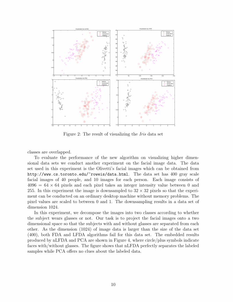
We test nLFDA, LFDA, LDA (conventional FDA) and PCA. Figure 2 shows thesamples of the Iris data set in the two-dimensional space found by each algorithm. Thehorizontal axis is the first feature found by each algorithm, while the vertical axis is thesecond feature. For this data set all the algorithms have nicely revealed the categories ofthe data.

In the second experiment, within four classes we select 789 samples from ’A’ class,766 samples from ’B’ class, 736 samples from ’C’ and 775 samples from ’F’ class. Wenote that the first two components found by both FDA and PCA algorithms do notseparate categorized samples well. In Figure 3 we therefore depict the samples of theLetter recognition data set in the three-dimensional space found by each algorithm. In thisexperiment, the conventional FDA algorithm finds only two discriminant components,hence we use a random direction as the third component in the picture. The view used ineach figure was found by rotating the space until a satisfactory visual effect was achieved.From the figures it is clearly seen that majority of samples from classes ’B’ and ’F’ aremixed in the result revealed by the FDA algorithm while only the samples from class ’A’are clearly separated from other class samples which are overlapped. Both nLFDA andLFDA revealed nice class structures in four classes although some samples from different

9

−10 −9 −8 −7 −6 −5 −4 −3 −2−7

−6.5

−6

−5.5

−5

−4.5

−4Visualization by nLFDA

SetosaVersicolourVirginica

0 50 100 150 200 25024

26

28

30

32

34

36

38

40

42

44Visualization by LFDA

SetosaVersicolourVirginica

−10 −8 −6 −4 −2 0 2 4 6 8 10−3

−2

−1

0

1

2

3Visualization by FDA

SetosaVersicolourVirginica

−4 −3 −2 −1 0 1 2 3 4−1.5

−1

−0.5

0

0.5

1

1.5Visualization by PCA

SetosaVersicolourVirginica

Figure 2: The result of visualizing the Iris data set

classes are overlapped.To evaluate the performance of the new algorithm on visualizing higher dimen-

sional data sets we conduct another experiment on the facial image data. The dataset used in this experiment is the Olivetti’s facial images which can be obtained fromhttp://www.cs.toronto.edu/~roweis/data.html. The data set has 400 gray scalefacial images of 40 people, and 10 images for each person. Each image consists of4096 = 64 × 64 pixels and each pixel takes an integer intensity value between 0 and255. In this experiment the image is downsampled to 32 × 32 pixels so that the experi-ment can be conducted on an ordinary desktop machine without memory problems. Thepixel values are scaled to between 0 and 1. The downsampling results in a data set ofdimension 1024.

In this experiment, we decompose the images into two classes according to whetherthe subject wears glasses or not. Our task is to project the facial images onto a twodimensional space so that the subjects with and without glasses are separated from eachother. As the dimension (1024) of image data is larger than the size of the data set(400), both FDA and LFDA algorithms fail for this data set. The embedded resultsproduced by nLFDA and PCA are shown in Figure 4, where circle/plus symbols indicatefaces with/without glasses. The figure shows that nLFDA perfectly separates the labeledsamples while PCA offers no clues about the labeled data.

10

−25

−20

−15

−10

−5

0 −15

−10

−5

0

−40

−20

0

20

Visualization by nLFDA

ABCF

50

100

150

200 0

10

20

30

40

50

60

70

80

90−100

−50

0

50

100

Visualization by LFDA

A

B

C

F

−8−6

−4−2

02

4

−6

−4

−2

0

2

4

6

−20

−10

0

10

Visualization by FDA

A

B

C

F

−15

−10

−5

0

5

10

15

−15

−10

−5

0

5

10

15

−10

0

10

Visualization by PCA

A

B

C

F

Figure 3: The result of visualizing the Letter recognition data set

−0.5 0 0.5 1 1.5 2 2.5 3 3.5−12

−11

−10

−9

−8

−7

−6

−5Visualization by nLFDA

Without GlassesWith Glasses

−6 −5 −4 −3 −2 −1 0 1 2 3 4−1

−0.5

0

0.5

1

1.5

2

2.5

3Visualization by PCA

Without GlassesWith Glasses

Figure 4: The result of visualizing Olivetti’s facial image data set

11

Data Sets nLFDA LFDA FDA PCA

Iris 3.17% (0.0253) 3.17% (0.0253) 4.67% (0.0274) 3.67% (0.0304)Letters 13.1% (0.0161) 13.0% (0.0161) 16.6% (0.0112) 32.8% (0.0167)

USPS Digits 7.74% (0.0032) 7.74% (0.0032) 7.24% (0.0041) 7.73% (0.0025)Olivetti’s faces 16.4% (0.0497) N/A N/A 24.4% (0.0296)

Table 1: Comparison on classification accuracy between these algorithms using 1-nearestneighbor criterion (the standard deviation appeared in parenthesis)

4.3 Classification

Here we apply the proposed new algorithm nLFDA, LFDA, LDA (conventional FDA)and PCA to classification tasks.

There are several measures for quantitatively evaluating separability of projected datasamples in different classes (Fukunaga, 1990). Here we use a simple one: misclassificationrate by a 1-nearest-neighbor criterion. We know the one-nearest-neighbor metric dependson the distance of projected data samples. To get consistent results, in our experimentswe use an orthogonal transform F as defined by Theorem 3.3, i.e., we take F as theorthogonal part of QR decomposition of X.

We use the same data sets in Section 4.2. In addition, we use the ten classes dataset created from the USPS handwritten digit data set. For the data sets IRIS, theembedding dimensionality is chosen as 2, while for other three data sets, the embeddingdimensionality is set to 9 in our experiments. Table 1 describes the mean and standarddeviation of the misclassification rate by each method on 10 fold experiments where thedata sets are split into training and testing sets at a ratio of 4 to 1. The table showsthat the overall performance of nLFDA is comparable to that of the LFDA, the latter ofwhich has excellent performance. The LFDA as well as FDA failed in the Olivetti’s facialimage data. In this case, we only have 400 data points while the dimensional of eachface image is 1024. This results in a singular between-class scatter matrix. However thenLFDA is designed to tackle this undersample problem. The performance of the nLFDAon this data set is much better than that of PCA.

5 Conclusions

In this paper we modify the formulation of the local Fisher Discriminant Analysis (LFDA)(Sugiyama, 2007) so that the new formulation is more robust for high dimensional datasets. When the data dimension is larger than the number of the size of a data set,the LFDA will fail due to the singularity of the within-class scatter matrix. Instead ofusing the matrix inverse in the formulation the pseudo-inverse is adopted in the newformulation. The new algorithm has a comparable capacity as the LFDA in most caseswhile it offers a robust implementation for higher dimensional data sets. A family ofsolutions to the new formulation has been derived based on a comprehensive analysis.The algorithm based on this analysis is robust in all the experiments.

12

In this paper we focused on the linear dimensionality reduction of the new algorithmand its application to data visualization. Obviously the new algorithm can be combinedwith other classifiers such as the 1-nearest-neighbor classifier for classification problems.

Acknowledgements

The authors are grateful to anonymous reviewers for their constructive advices.

References

Asuncion, A. and D. Newman (2007). UCI machine learning repository. Uni-versity of California, Irvine, School of Information and Computer Sciences,http://www.ics.uci.edu/∼mlearn/MLRepository.html.

Caillault, E. and C. Viard-Gaudin (2007). Mixed discriminant training of hybridann/hmm systems for online handwritten word recognition. International Journalof Pattern Recognition and Artificial Intelligence 21, 117–134.

Duda, R., P. Hart, and D. Stork (2001). Pattern Classification (2nd ed.). New York:John Wiley and Sons.

Fisher, R. (1936). The use of multiple measurements in taxonomic problems. Annals ofEugenics 7 (2), 179–188.

Fukunaga, K. (1990). Introduction to Statistical Pattern Recognition (2nd ed.). Boston:Academic Press.

Golub, G. and C. van Loan (1996). Matrix Computations (3 ed.). Maryland: The JohnsHopkins University Press.

Guo, Y., J. B. Gao, and P. W. Kwan (2006). Visualization of non-vectorial data using twinkernel embedding. In K. Ong, K. Smith-Miles, V. Lee, and W. Ng (Eds.), Proceedingsof the International Workshop on Integrating AI and Data Mining (AIDM 2006) inAustralia, pp. pp11–17. IEEE Computer Society.

Guo, Y., J. B. Gao, and P. W. Kwan (2008). Twin kernel embedding. IEEE Transactionon Pattern Analysis and Machine Intelligence 30, 1490–1495.

Ham, J., Y. Lin, and D. Lee (2005). Learning non-linear appearance manifolds forrobot localization. In Proceedings of IEEE/RSJ International Conference on IntelligentRobots and Systems, pp. 2971–2976.

He, X. and P. Niyogi (2004). Locality preserving projections. In S. Thrun, L. Saul, andB. Scholkopf (Eds.), Advances in Neural Information Processing Systems, Volume 16,Cambridge, MA. MIT Press.

13

Jin, Z., J. Yang, Z. Hu, and Z. Lou (2001). Face recognition based on the uncorrelateddiscriminant transformation. Pattern Recognition 34, 1405–1416.

Mekuz, N., C. Bauckhage, and J. Tsotsos (2005). Face recognition with weighted locallylinear embedding. In Proceedings of the 2nd Canadian Conference on Computer andRobot Vision, pp. 290–296.

Miguel, L., G. Phillips, and L. Kavraki (2002). A dimensionality reduction approach tomodeling protein flexibility. In Proceedings of International Conference on Computa-tional Molecular Biology, pp. 299–308.

Okun, O., H. Priisalu, and A. Alves (2005). Fast non-negative dimensionality reduc-tion for protein fold recognition. In Proceedings of European Conference on MachineLearning, 665-672.

Paige, C. and M. Saunders (1981). Towards a generalized singular value decomposition.SIAM Journal on Numerical Analysis 18, 398–405.

Raytchev, B., I. Yoda, and K. Sakaue (2006). Multiview face recognition by nonlin-ear dimensionality reduction and generalized linear models. In Proceedings of the 7thInternational Conference on Automatic Face and Gesture Recognition (FGR06), Wash-ington, DC, USA, pp. 625–630.

Scholkopf, B. and A. Smola (2002). Learning with Kernels. Cambridge, Massachusetts:The MIT Press.

Sugiyama, M. (2007). Dimensionality reduction of multimodal labeled data by local fisherdiscriminant analysis. Journal of Machine Learning Research 8, 1027–1061.

Turk, M. and A. Pentland (1991). Eigenfaces for recognition. Journal of Cognitive NeuroScience 3 (1), 71–86.

Uchyigit, G. and K. Clark (2007). A new feature selection method for text classification.International Journal of Pattern Recognition and Artificial Intelligence 21, 423–438.

van der Maaten, L., E. O. Postma, and H. van den Her-ick (2007). Dimensionality reduction: A comparative review.http://www.cs.unimaas.nl/l.vandermaaten/dr/DR draft.pdf.

Ye, J. (2005). Characterization of a family of algorithms for generalized discriminantanalysis on undersampled problems. Journal of Machine Learning Research 6, 483–502.

Ye, J. and T. Xiong (2006). Computational and theoretical analysis of null space andorthogonal linear discriminant analysis. Journal of Machine Learning Research 7,1183–1204.

Zhao, D., Z. Lin, R. Xiao, and X. Tang (2007). Linear laplacian discrimination for featureextraction. In Proceedings of IEEE Conf. on Computer Vision and Pattern Recognition(CVPR’07).

14