PCA R&D SN2863

Thickness Design Systems for Pavements Containing Soil-Cement

Bases

by Tom Scullion; Jacob Uzan; Stacy Hilbrich, and Peiru Chen

©Portland Cement Association 2008 All rights reserved

ii

KEYWORDS Mechanistic pavement design, soil-cement, thickness design, resilient modulus ABSTRACT With the proposed move to a national Mechanistic Empirical Pavement Design Guide (MEPDG) the Portland Cement Association (PCA) initiated this study to review the proposed models for Soil-Cement (S-C) base and Cement Modified Soils (CMS). To provide a smooth transition to the new design procedures researchers evaluated the laboratory procedures needed to provide the input material properties for resilient modulus (MR) and modulus of rupture (Mr). In addition, software tools were developed to introduce the concepts of mechanistic design to pavement designers. Researchers found that the traditional laboratory resilient modulus test is extremely difficult to run on S-C samples. The induced strains are very low, and the sample preparation and finishing have a major impact on repeatability. A new test including measurement of the seismic velocity appears to provide much more potential. A good correlation was obtained between both tests. The use of unconfined compressive strength to estimate both resilient modulus and modulus of rupture also appears reasonable. Recommendations are provided in this report. A summary was also made of tools for measuring resilient modulus in the field. The use of the Falling Weight Deflectometer (FWD), Portable Seismic Pavement Analyzer, and lightweight FWD are described. From FWD data, the resilient modulus values obtained in the field are substantially less than those measured in the laboratory. To evaluate the proposed MEPDG model for S-C bases, an attempt was made to calibrate the model with accelerated pavement test data collected by the PCA in the 1970’s. Calibration factors were developed for the proposed model. In addition, a model based on the PCA recommendations was also calibrated. Both calibrated models were built into two software packages developed in this study. These packages are intended as training tools for introducing the concept of handling the S-C or CMS layer in mechanistic-empirical design systems. REFERENCE Scullion, Tom; Uzan, Jacob; Hilbrich, Stacy, and Chen, Peiru, Thickness Design Systems for Pavements Containing Soil-Cement Bases, SN2863, Portland Cement Association, Skokie, Illinois, USA, 2008, 95 pages.

iii

TABLE OF CONTENTS

Page

Keywords ........................................................................................................................................ ii Abstract ........................................................................................................................................... ii Reference ........................................................................................................................................ ii List of Figures ................................................................................................................................ iv List of Tables ...................................................................................................................................v Chapter 1. Introduction ....................................................................................................................1

Project Description ..............................................................................................................2 Goals of This Report ............................................................................................................5

Chapter 2. Evaluation of Laboratory Procedures for Measuring Moduli Values for S-C Materials ............................................................................6

Background ..........................................................................................................................6 Repeatability Measurements on Laboratory Moduli Values .............................................13 Summary and Recommendations ......................................................................................21

Chapter 3. Case Study: Determining Input Values for the Design Guide .....................................22 Specimen Preparation ........................................................................................................22 Test Results and Discussion ..............................................................................................23 Relationships Between Testing Procedures .......................................................................33 Summary ............................................................................................................................36

Chapter 4. Moduli Measurements in the Field .............................................................................38 Falling Weight Deflectometer............................................................................................38 Portable Seismic Pavement Analyzer ................................................................................44 PRIMA 100 ........................................................................................................................47 Dynamic Cone Penetrometer .............................................................................................49

Chapter 5. A Mechanistic Empirical Thickness Design Program for Pavements with S-C Bases or Cement Modified Soils ......................................................51 Background ........................................................................................................................51 Calibration of the Model ....................................................................................................56 Verification and Case Studies ............................................................................................60

Chapter 6. Conclusions and Recommendations.............................................................................67 Conclusions ........................................................................................................................67 Recommendations for Implementation ..............................................................................69

Acknowledgment ...........................................................................................................................71 References ......................................................................................................................................72 Appendix A. PCA Performance Results Used for Model Calibration ..........................................73 Appendix B. User’s Manual for the CTB Computer Thickness Design Program .........................76 Appendix C. User’s Guide for Stress Analysis Training Program ................................................83

iv

LIST OF FIGURES

Page 1. Input interface of stabilized materials .........................................................................................4 2. Seismic modulus testing .............................................................................................................6 3. Typical seismic test result screen ................................................................................................7 4. Dynamic modulus testing loading wave .....................................................................................9 5. Setup of LVDTs in dynamic modulus test ................................................................................10 6. Dynamic modulus testing frame ...............................................................................................10 7. Typical dynamic modulus test result screen .............................................................................11 8. Strains under repeated loads in resilient modulus testing .........................................................12 9. MTS setup for resilient modulus test ........................................................................................12 10. Six soil-cement 4 x 8-in. samples ............................................................................................14 11. Dynamic moduli at different rrequencies ................................................................................16 12. Soil-cement 4 x 8-in. samples ..................................................................................................19 13. Relationship between resilient and dynamic moduli ...............................................................20 14. Molded beam specimen for modulus of rupture ......................................................................23 15. Setup of free-free resonant column test ...................................................................................24 16. Sample preparation for the resilient modulus test ...................................................................27 17. Displacement in LVDT 7 for Sample 6x8B at day 7 ...............................................................29 18. Displacement in LVDT 8 for Sample 6x8B at day 7 ...............................................................29 19. Displacement in LVDT 7 for Sample 6x12D at day 7 .............................................................30 20. Displacement in LVDT 8 for Sample 6x12D at day 7 .............................................................30 21. Third-point loading of a simple beam ......................................................................................32 22. Comparison of low-strain resilient modulus to seismic modulus ............................................34 23. Comparison of resilient modulus to UCS ................................................................................35 24. Comparison of modulus of rupture to 28-day UCS .................................................................36 25. Falling weight deflectometer ...................................................................................................38 26. Moduli calculation screen in modulus software ......................................................................39 27. Summary of gain of modulus with time ..................................................................................42 28. Core from the test pavement after 3 years in service ...............................................................42 29. Portable seismic pavement analyzer (Nazarian 2006) .............................................................44 30. Typical time records from PSPA (Nazarian 2006) ..................................................................45 31. Schematic of USW method ......................................................................................................46 32. PSPA used to collect seismic modulus of S-C layers in the field ............................................46 33. Field data collected with the PSPA on a S-C Base near Odessa, Texas (Nazarian 2006) .......47 34. Prima 100 .................................................................................................................................48 35. Comparing base moduli from the FWD and Prima .................................................................48 36. DCP Testing .............................................................................................................................49 37. Structural section with S-C layers ...........................................................................................52 38. Fatigue relationships in the CTB Program ..............................................................................55 39. Calibration for granular soil-cement for Design Guide and exponential models ....................59 40. Calibration for fine-grained soil-cement ..................................................................................60

v

LIST OF TABLES

Page

1. Material Sieve Results ..............................................................................................................13 2. Dynamic Modulus@30 psi, 10 Hz (ksi) ...................................................................................14 3. Dynamic Modulus@20 psi (3 days), 50 psi (7, 14, 28 days), 10 Hz (ksi) ................................15 4. Dynamic Modulus@50 psi (3 days), 70 psi (7, 14, 28 days), 10 Hz (ksi) ................................15 5. Resilient Modulus @30 psi, 1 Hz (ksi) .....................................................................................17 6. Resilient Modulus@20 psi (3 days), 50 psi (7, 14, 28 days), 1 Hz (ksi) ..................................17 7. Resilient Modulus@70 psi (3 days), 70 psi (7, 14, 28 days), 1 Hz (ksi) ..................................18 8. Seismic Modulus Test Results (ksi) ..........................................................................................19 9. Comparison among Seismic, Dynamic, and Resilient Moduli .................................................20 10. UCS Test Results .....................................................................................................................21 11. Comparison of Three Modulus Test Methods .........................................................................21 12. Wet-Sieve Analysis of Limestone Aggregate ..........................................................................22 13. Seismic Modulus Test Results for 6 x 8-in. Samples (ksi) ......................................................24 14. Seismic Modulus Test Results for 6 x 12-in. Samples (ksi) ....................................................24 15. Seismic Modulus Test Results for 4 x 8-in. Samples (ksi) ......................................................25 16. Seismic Modulus Test Results for 4 x 4.5-in. Samples (ksi) ...................................................25 17. Resilient Modulus Test Results for 6 x 8-in. Samples (ksi) ....................................................27 18. Resilient Modulus Test Results for 6 x 12-in. Samples (ksi) ..................................................28 19. Resilient Modulus Test Results for 4 x 8-in. Samples (ksi) ....................................................28 20. Resilient Modulus (ksi) for Each LVDT .................................................................................31 21. UCS Test Results .....................................................................................................................32 22. Modulus of Rupture .................................................................................................................33 23. FWD Data Collected Shortly after Placement of S-C .............................................................41 24. FWD Data Collected after 3 Years in Service .........................................................................43 25. Minimum Values of 7 Days Unconfined Compressive Strength, for Cement Stabilized Materials, Units in psi in the Proposed New Design Guide ...................................53 26. Summary of Recommendations by the Design Guide, Units in psi ........................................53 27. Summary of Results for the Calibration of Granular Soil-cement ..........................................58 28. Summary of Results for the Calibration of Fine-Grained Soil-cement ...................................58 29. Default Properties for Soil-cement ..........................................................................................58 30. Summary of Results for Design Example 1 (from PCA 1970)................................................62 31. Summary of Results for Case 1 (from Larsen et al. 1969) ......................................................63 32. Summary of Results for Case 2 (from Larsen et al. 1969) ......................................................64 33. Summary of Results for Case 3 (from Larsen et al. 1969) ......................................................65 34. Summary of Results for Case 4 (from Larsen et al. 1969) ......................................................66

1

Thickness Design Systems for Pavements Containing Soil-Cement

Bases

by Tom Scullion, Jacob Uzan, Stacy Hilbrich, and Peiru Chen*

CHAPTER 1 INTRODUCTION The National Cooperative Highway Research Program (NCHRP) is in the final stages of developing and implementing a new Mechanistic Empirical Pavement Design Guide (MEPDG) to be used by all State Highway Agencies for layer thickness calculations (ARA 2004). For the first time this procedure will be mechanistically based with the design life for the soil-cement S-C base computed from flexural fatigue considerations. The material property to be used in design will be the resilient modulus value of the S-C base, the modulus of rupture, and Poisson’s ratio. The resilient modulus can be obtained either from dynamic laboratory testing or backcalculated from deflection data collected with Falling Weight Deflectometers (FWD). Frequently with S-C bases arbitrary factors are also included in the design process to reduce their modulus value to account for shrinkage cracking and/or traffic-induced damage. In the analysis procedure the tensile strains induced at the bottom of the S-C layer by the design wheel load are computed using a layered elastic program. These are then used to calculate the pavement life in terms of the number of repetitions required to cause load associated slab cracking. It is important to realize that this is a major national development effort but to date the focus of the NCHRP Project 1-37 team has been on asphalt stabilized and granular base materials, and little consideration has been given to soil-cement bases or the benefits of Cement Modified Soils (CMS). This new design approach presents both opportunities and challenges to the cement industry. S-C bases typically have high moduli values, often 10 to 20 times that of unstabilized granular materials. However, with S-C bases it is also important to safeguard against under-design where thin structures are proposed, which may fatigue quickly under heavy truck loads. Once the new MEPDG is adopted by the American Association of State Highway and Transportation Officials (AASHTO), it will become the national procedure that will be required on all federally aided projects. It is important that realistic design moduli values be used for both S-C bases and CMS subgrades. It is important for the Portland Cement Association (PCA) to gear up for both the opportunities and challenges that this potential major change will provide. The goal of this research project is to prepare the PCA for this new design procedure, to document existing practices with mechanistic design, to develop recommendations on how to measure resilient modulus in the lab and field, and to develop realistic values for a range of both * Senior Research Engineer, Research Engineer, Assistant Research Engineer, and Research Assistant, Texas Transportation Institute, The Texas A&M University System, College Station, Texas, USA, 77843-3135.

2

S-C bases and CMS subgrades. The concepts to be used in the new design procedure are not widely known to the cement industry or most highway agencies. The goal of the research presented in this report is to review the design concepts and to document how the input values can be obtained from either lab or field testing. Furthermore, the design software is a large integrated package, which may be difficult for the novice designer to navigate. To aid in the transition to mechanistic based design, researchers developed two design tools in this study. The models used within these programs are identical to the model included in the proposed MEPDG. In this study the research team developed a model calibration procedure. The proposed calibration factors are based on accelerated pavement testing data collected by PCA in the 1970’s. The first design tool is a stress analysis program (CTBana), which permits designers to calculate stresses and strains in pavements with S-C base or subbase layers. The number of repetitions to failure under the design load is then calculated. The program also lets the designer input other base types for comparison. The second tool is a design system, which computes the number of repetitions of loads required for the stabilized base or subbase to experience fatigue damage. This program is more comprehensive as it permits the input of mixed traffic streams. PROJECT DESCRIPTION

Input Request for New NCHRP Project 1-37 Design Guide Development of the new NCHRP Guide for the Design of New and Rehabilitated Pavement Structures is the goal of the research and development efforts of NCHRP Project 1-37A. The new NCHRP Project 1-37 Design Guide is anticipated to become the latest and most significant revision of the AASHTO Design Guide. The pavement design methodology is based on mechanistic principles, which will allow more efficient use of paving materials, improve pavement performance, and decrease life cycle costs. Although the new guide was originally scheduled for release in 2002, as of late 2007 the new design guide system was still under review. The initial version was found to have several problems. A revised version (0.8) was scheduled for release in late 2005, and version 0.9, which will contain further improvements and recalibrated performance models, was scheduled for release in mid-2006. While complete details of the final version of the new procedure are not known, it is anticipated that it will provide pavement engineers with three design options with different levels of sophistication. At the highest level (1), designs will involve extensive laboratory testing of all the materials in each layer of the pavement. For all layers the primary design values will be the Resilient Modulus and the Poisson Ratio. In level 2 designs the material properties will be obtained from standard test results such as unconfined compressive strength (UCS). Level 3 designs will involve table look ups. It is anticipated that the vast majority of designs will be either levels 2 or 3 with level 1 restricted to research or a few major projects. As for the S-C layer, the NCHRP Design Guide mainly takes load associated fatigue damage into consideration. A sigmoidal function in Equation 1 is used to evaluate the fatigue performance of the S-C layer.

3

⎥⎥⎥⎥⎥⎥

⎦

⎤

⎢⎢⎢⎢⎢⎢

⎣

⎡

β⎥⎥⎦

⎤

⎢⎢⎣

⎡ δ−β

=

2c2

rup

s1c1

k

Mk

10fN (1)

where

Nf = number of repetitions to fatigue cracking,

δs = tensile stress (psi) at the bottom of S-C layer,

Mrup = modulus of rupture (psi), and

k1, k2, βc1, and βc2 = regression/calibration coefficients.

In this fatigue equation, δs is computed based on the elastic layer theory with the resilient

modulus of the S-C layer being the most significant material property. As with all other S-C models, the key design parameter is the ratio of induced stress to the modulus of rupture (specified as that measured after 28 days). The modulus of rupture (Mrup) can be directly measured in the laboratory or taken from the UCS based on the existing relationship between Mrup and UCS. Thus, the main S-C material properties needed include resilient modulus and modulus of rupture.

In addition, the effects of age, thermal property, and fracture of the S-C on resilient modulus are considered. In the new Design Guide, the input interface of the S-C layer is shown in Figure 1.

To avoid confusion of the Modulus of Rupture will defined by the symbol Mrup, whereas the Resilient Modulus will use the traditional symbol Mr.

4

Figure 1. Input interface of stabilized materials (ARA 2004).

The input information needed in the NCHRP Project 1-37 Design Guide includes three types of properties: general properties, strength properties, and thermal properties. General properties are composed of the layer thickness of the S-C layer, unit weight, and Poisson’s ratio. The Poisson’s ratio can be defined as a constant, for example, 0.2.

The strength properties are key properties for the S-C layer. They consist of resilient modulus, minimum resilient modulus, and modulus of rupture (all measured after 28 days). The resilient modulus is a key factor for fatigue cracking analysis as it is used to calculate the tensile stress at the bottom of the S-C layer (δs). The new Guide assumes under traffic loads the modulus of the S-C layer will decrease to a minimum value over time. For S-C the latest version of the Guide recommends initial and final moduli values of 500 ksi and 50 ksi. This implies that over the life of the pavement the moduli of the S-C layer will decrease by a factor of 10. This is a very conservative assumption which is not supported by long term performance studies.

Another critical parameter for fatigue analysis is the modulus of rupture. It can be directly measured from laboratory tests (ASTM D1635). However, in most circumstances it is determined by the existing relationship between the modulus of rupture and UCS. For example, the following equations have been developed to establish the relationship.

American Concrete Institute (ACI): cr ff '5.7= (2)

(for Concrete, fr refers to the modulus of rupture and f’c refers to the UCS)

5

U. S. Army Corps of Engineers (USACE): UCS0459.9M rup = (3)

(for Concrete, Mrup refers to the modulus of rupture)

Further discussion of the strengths and weaknesses of the proposed model will be presented in Chapter 5 of this report. While the current model recommends a decrease in the modulus with time it does not change the modulus of rupture. It is difficult to understand why one material property would change and the other would remain fixed. The final input properties are thermal properties including thermal conductivity and heat capacity, which are useful in explaining the thermal contraction of S-C. These properties are not widely used and will most likely be obtained from table look ups.

In summary, the main engineering properties the new NCHRP Project 1-37 Design Guide needs are the resilient modulus and the modulus of rupture. The resilient modulus can be determined either in the laboratory or in the field. The approaches to determine the resilient modulus will be discussed in the following two chapters. GOALS OF THIS REPORT The purpose of this project is to:

• conduct laboratory tests to determine layer moduli values for S-C materials, • provide recommendations to PCA on how the required input values can be obtained from

commonly run laboratory tests such as the UCS, and • develop Windows-based tools, which will perform mechanistic analysis of multilayer

pavement layer structures. These simple tools can be used to introduce designers to the concepts inside the new MEPDG.

In Chapter 2 of this report, the commonly used methods of determining the resilient

modulus properties of S-C base materials are discussed. A new procedure using seismic equipment is also described. In Chapter 3 a case study is presented to discuss how the input requirements for the new Guide can be determined in the laboratory. A review is also made of the method of obtaining design values from 7-day UCS. Regression equations are established to relate the UCS values to both design moduli values and the modulus of rupture.

In Chapter 4 a description is given of the methodologies used to obtain moduli values using nondestructive testing technologies.

Chapter 5 presents the Windows-based tools for performing mechanistic analysis and for training State Highway Agencies (SHA) personnel in the basics of the new design concepts. Two programs were developed. The first is a simple training tool for computing stresses and strains within a multilayered system. The second is a more complete design program in which the user can input mixed traffic and estimate the fatigue damage. In both programs, two main performance models are proposed. The first is the model proposed in the new Design Guide. The second is a fatigue model based on the PCA existing fatigue damage model. A unique feature of this work is the development of calibration factors for these models. This is based on accelerated pavement tests conducted by PCA in the late 1960’s. User guides for these models are provided in Appendix B and C of this report.

6

CHAPTER 2 EVALUATION OF LABORATORY PROCEDURES FOR MEASURING MODULI VALUES FOR S-C MATERIALS Background

In this chapter, three different methods of measuring the resilient modulus in the laboratory are compared and contrasted. Each method is described below: Method 1: Seismic Modulus. The seismic modulus was measured using the free resonant column method. This procedure for testing highway materials has been researched extensively at the University of Texas at El Paso (Nazarian et al. 2002). As shown in Figure 2, a cylindrical specimen is placed on its side on a sheet of foam in the laboratory, and seismic waves are induced by tapping the sample with a hammer equipped with a load cell that measures the energy input and triggers a timing circuit. An accelerometer mounted to the other end of the sample reports the time of P-wave arrival.

Figure 2. Seismic modulus testing.

A computer displays the measured wave response shape, which is used to determine the quality of the test data. The computer screen is shown in Figure 3. It is very easy to get the resonant frequency from the small window on the left side of the screen. The seismic modulus can be calculated from measured P-wave velocities and the known density of the material according to Equation 4:

7

2pVE ⋅= ρ (4)

where E = seismic modulus (MPa); ρ = density (Kg/m3); and

pV = P-wave velocity (m/s).

The equation for calculating P-wave velocity from the P-wave frequency measured with the seismic resonant column is below:

LFVp ⋅⋅= 2 (5) where

F = P-wave frequency (Hz); and L = Length of the specimen (m).

Figure 3. Typical seismic test result screen.

The seismic test takes less than three minutes to complete. In Figure 3, the screen shows the typical seismic modulus test results. The initial peak marked with a (+) signifies the frequency of the P-wave as it passes through the sample. The sample shown in Figure 2 was capped as this sample was also to be tested with the dynamic or resilient modulus tests. However, caps are not typically needed or necessary for the seismic modulus test.

8

Method 2: Dynamic Modulus. The complex modulus, E*, is defined as a complex number that relates stress to strain for a linear viscoelastic material subjected to a sinusoidal loading. The absolute value of the complex modulus, *E , is commonly referred to as the dynamic modulus. The dynamic modulus test equipment is being developed to provide the main material input to the new NCHRP design software (ARA 2004). All hot mix asphalt (HMA) layers are to be characterized with this equipment. In this study the same equipment is used to measure the dynamic modulus of the S-C samples.

Dynamic modulus values are normally conducted on unconfined specimens using a uniaxially applied sinusoidal (haversine) stress pattern. Through recording equipment, axial strains are continuously monitored throughout the test. As shown in Figure 4, the sinusoidal stress σ is:

( )tωσσ sin0= (6) where

0σ = the stress amplitude; ω = the angular frequency (radian per second); and t = the time (second). The resultant sinusoidal strain ε is:

( )ϕωεε −= tsin0 (7) where

0ε = the recoverable strain amplitude; ϕ = the phase lag (degree); and

ϕ = the phase angle is simply the angle at which the 0ε lags 0σ or:

( )°= 360p

i

tt

ϕ (8)

where

it = the time lag between a cycle of sinusoidal stress and a cycle of strain (sec); and pt = the time for a stress cycle (sec).

By definition, the complex modulus *E is: "'* iEEE += (9)

where

ϕ

εσ

cos0

0' =E and refers to the real portion of the complex modulus;

ϕεσ

sin"0

0=E and refers to the imagination portion of the complex modulus; and

i = an imagination number.

9

For elastic material such as S-C, 0=ϕ , it can be seen that

0

0**

εσ

== EE (10)

Thus, as noted, the elastic or dynamic modulus of S-C material may be determined by the

ratio of the peak stress to strain amplitudes from the complex modulus test. In this report, the standard test method for the dynamic modulus of asphalt concrete

mixtures (NCHRP 1-37A draft test method DM-1) was used to measure the dynamic modulus of S-C materials. The dynamic modulus was determined over a range of frequencies from 1 to 25 Hz, with the sinusoidal stress amplitude held at 30 psi, 50 psi, and 70 psi. As shown in Figure 5, linear variable differential transformers (LVDTs) were employed to continuously record the uniaxial strain over the middle of the specimen. The gage length is 4 in. for the 8-in. height sample as recommended by AASHTO. At each frequency, 200 load repetitions are applied, and the last five load repetitions are used to compute the dynamic modulus in the unconfined state.

The setup time for this test is about one hour, which includes capping the sample and adjusting the equipment. Testing, at three load levels and using four frequencies for each level, takes about half an hour. The equipment for the dynamic modulus test is shown in Figure 6, and its cost is about $40,000. As shown in Figure 7, during the test the response of the LVDTs and load cell are reported, and the dynamic modulus can be automatically determined by the associated software.

Figure 4. Dynamic modulus testing loading wave.

10

Figure 5. Setup of LVDTs in dynamic modulus test.

Figure 6. Dynamic modulus testing frame.

11

Figure 7. Typical dynamic modulus test result screen. Method 3: Resilient Modulus. It is well known that most paving materials are not elastic but experience some permanent deformation after each load application. However, if the load is small compared to the strength of the material and is repeated for a large number of times, the deformation under each load repetition is nearly completely recoverable and proportional to the load, and can be considered as elastic. This assumption is certainly true for S-C base materials.

When an HMA specimen is under a repeated load, at the initial stage of load applications there is considerable permanent deformation that is depicted in Figure 8. As the number of load repetitions increases, the plastic strain due to each load repetition decreases. After 100 to 200 repetitions, the strain is practically recoverable.

The elastic modulus based on the recoverable strain under repeatable loads is called the resilient modulus Mr, defined as:

r

drM

εσ

= (11)

where dσ = the deviator stress; and

rε = the recoverable strain. The standard method of testing for the resilient modulus of subgrade soils and untreated

base/subbase materials (AASHTO DESIGNATION T 292-91) was used to measure the resilient modulus. In this test, with a repeated axial deviator stress amplitude held at 30 psi, 50 psi, and 70 psi, 0.1 s load and 0.9 s unload cycle is applied to an unconfined specimen. The total resilient axial strain of each specimen after a 200-cycle conditioning period is measured with LVDTs, and the results from the last five cycles are used to calculate the resilient modulus. The setup time for

12

this test is about one hour, which includes capping the sample and adjusting the equipment. When testing, three load levels take about 15 minutes. The resilient modulus test was conducted using the material test system (MTS) machine. This machine costs about $350,000 and is illustrated in Figure 9.

Figure 8. Strains under repeated loads in resilient modulus testing.

Figure 9. MTS setup for resilient modulus test.

Difference between Resilient and Dynamic Moduli. The difference between the resilient modulus test and the dynamic modulus test is that the former uses loadings typically haversine with a given rest period, while the latter applies a sinusoidal or haversine loading with no rest period. For the viscoelastic materials, the rest period will increase the recoverable deformation, which leads to a smaller resilient modulus compared to the dynamic modulus. However, in an elastic material such as the S-C base, there is no time lag between stress and strain. Thus, the

13

resilient modulus should be equal to the dynamic modulus. Based on the existing knowledge of elasticity of the S-C material, the resilient modulus should be close to the dynamic modulus. Repeatability Measurements on Laboratory Moduli Values To demonstrate these different procedures and the variability in results, researchers conducted a series of tests on typical S-C materials. Specimen Preparation. A limestone aggregate base material was used for evaluation of the test repeatability. The optimum moisture content was found to be 7.0 %. The results of a mechanical sieve analysis are given in Table 1. For sample preparation, the aggregates larger than ¾-in. were scalped, and specimens were compacted in four lifts of 22 blows each with a 10-lb hammer dropped from a height of 18 in. to a finished diameter of about 4 in. inside an 8-in. high steel mold.

As shown in Figure 10, six replicate specimens were molded in this manner at 3% portland Type I cement (by dry weight), where the compaction moisture was increased 0.25% for each 1.0% cement added to the specimen.

After the compaction, molded specimens were placed in the moisture room for curing. Then seismic modulus, dynamic modulus, resilient modulus, and UCS tests were conducted after different curing times.

Table 1. Material Sieve Results

Sieve Size Sieve Size(mm)

Retained Weight(g) %Retained % Passing

3/4-in. 19.000 8286.5 14.7 85.3

3/8-in. 9.500 10758.5 19.1 66.2

No. 4 4.750 7573.5 13.4 52.8

No. 10 2.000 6680.6 11.9 40.9

No. 40 0.425 9206.3 16.3 24.6

No. 100 0.150 9716.8 17.3 7.3

No. 200 0.075 3366.4 6.0 1.3

Pan Pan 754.7 1.3 0.0

14

Figure 10. Six soil-cement 4 x 8-in. samples.

Test Results and Discussion. One sample designated as 702-5 was damaged during extrusion from the mold. The sample was included in the tests reported below; however, its results are typically lower than the other samples so that its results are excluded from the statistical analysis. Dynamic Modulus Test Results. Though dynamic modulus tests were run at frequencies of 1, 5, 10, and 25 Hz at room temperature (77 °F), the results of the 10 Hz load frequency at three loading levels are discussed in this report, since 10 Hz is the frequency most referenced in many of the test protocols. Also, test results show the moduli value for S-C materials is not frequency dependent.

The dynamic modulus also was measured at different curing times and at different load levels. Table 2 shows the results tested at the load of 30 psi. It can be seen that most of the modulus data show an increasing trend along with the curing days. Table 2 presents the statistical analysis results. For the dynamic modulus, the mean value of the coefficient of variation is 13.5%.

Table 2. Dynamic Modulus@30 psi, 10 Hz (ksi)

Curing Days 3 7 14 28

702-1 1137 1192 1283 1250

702-2 1134 1262 1300 1413

702-3 1181 1450 1416

702-4 1169 1254 1249 1668

702-5* 829 1077 1112 1310

702-6 1450 1448 1701 2008

Range 1140~1450 1190~1450 1250~1700 1250~2000

Av. 1214 1321 1390 1585

S.D. 133 120 185 331

C.V. 11% 9% 13% 21% *Sample damaged during extrusion from mold.

15

Similarly, Table 3 shows the results tested at 50 psi. The modulus generally increases with the increased curing time. For the dynamic modulus, the mean value of the coefficient of variation is 13.3%. The range of the dynamic modulus at 28 days under the load of 50 psi is 1200~1800 ksi, which is a little bit lower than that under the load of 30 psi. Table 3. Dynamic Modulus@20 psi (3 days), 50 psi (7, 14, 28 days), 10 Hz (ksi)

Curing Days 3 7 14 28

702-1 1174 1442 1155 1201

702-2 1250 1171 1238 1350

702-3 1230 1460 1702

702-4 1081 1168 1292 1419

702-5* 996 1061 1139 1186

702-6 1303 1447 1477 1830

Range 1080~1300 1170~1500 1160~1700 1200~1800

Av. 1208 1338 1373 1450

S.D. 84 154 219 269

C.V. 7% 11% 16% 19% *Sample damaged during extrusion from mold.

Table 4 shows the results tested at 70 psi. Similarly, most of the modulus data show an increasing trend along with the curing days. It was also found that the dynamic modulus at 28 days under the load of 70 psi ranged from 1320~1700 ksi, almost the same as that under the 50 psi load level. The mean value of the coefficient of variation is 10%. Table 4. Dynamic Modulus@50 psi (3 days), 70 psi (7, 14, 28 days), 10 Hz (ksi)

Curing Days 3 7 14 28

702-1 1070 1301 1256 1456

702-2 1018 1160 1207 1322

702-3 1102 1484 1734

702-4 1075 1140 1323 1426

702-5* 830 981 1163 1177

702-6 1168 1407 1525 1699

Range 1020~1200 1140~1500 1200~1520 1320~1700

Av. 1087 1298 1409 1447

S.D. 54 150 218 108

C.V. 5% 12% 15% 7% *Sample damaged during extrusion from mold.

16

As shown in Figure 11, the frequency of loading has no significant effect on the modulus. This indicates that under these loading conditions the S-C base behaves as an elastic material. Thus, the measured dynamic modulus ought to be equivalent to the resilient modulus and can represent the elastic property of the S-C base as the input to the MEPDG.

Figure 11. Dynamic moduli at different frequencies.

There was a change in the resilient modulus with a change in load level. At 28 days at the three load levels of 30, 50, and 70 psi, the average dynamic modulus changed from 1585 ksi to 1450 ksi to 1447 ksi. The slightly higher value at 30 psi is attributed to the low load level. At 30 psi very small movements are induced in the LVDTs around the sample. This load level is potentially not high enough to get a measurement of induced strain. At the higher level, the measured modulus becomes constant at around 1450 ksi.

Resilient Modulus. The Resilient modulus also was measured under three loading levels (30 psi, 50 psi, and 70 psi) at room temperature (77°F). The test results at 30 psi are shown in Table 5. It can be seen that most of the modulus data except some tested at 7 and 14 days show an increasing trend along with the curing days. The range of the resilient modulus at 28 days is 1300~2600 ksi.

500

1000

1500

2000

2500

0 5 10 15 20 25 30

Frequency(Hz)

Dyna

mic

Mod

ulus

(ksi

)

17

Table 5. Resilient Modulus @30 psi, 1 Hz (ksi) Curing Days 3 7 14 28

702-1 1377 1196 1376 2037

702-2 1244 1136 1176 1295

702-3 1131 1210 1283 1418

702-4 972 1223 1158 1897

702-5* 486 1107 525 1168

702-6 1130 1165 1858 2608

Range 1130~1400 1140~1220 1160~1850 1300~2600

Av. 1171 1186 1370 1851

S.D. 151 35 286 526

C.V. 13% 3% 21% 28% *Sample damaged during extrusion from mold.

Table 6 shows the test results at the load of 50 psi. Most of the modulus data do not show an apparently increasing trend along with the curing days. For the resilient modulus, the mean value of the coefficient of variation becomes higher to 19.3%. The range of the resilient modulus at 28 days is 1080~1350 ksi, which is lower than the modulus tested at 30 psi. Table 6. Resilient Modulus@20 psi (3 days), 50 psi (7, 14, 28 days), 1Hz (ksi)

Curing Days 3 7 14 28

702-1 1945 1139 1640 1081

702-2 1360 1125 1115 1216

702-3 1161 1382 1292 1231

702-4 936 1224 907 1345

702-5* 530 833 530 1170

702-6 1060 1165 1887 1200

Range 1060~2000 1130~1400 1120~1900 1080~1350

Av. 1292 1207 1368 1215

S.D. 396 105 395 94

C.V. 31% 9% 29% 8% *Sample damaged during extrusion from mold.

Table 7 shows the test results at 70 psi. It can be seen that most of the data do not show a seemingly increasing trend along with the curing days. For the resilient modulus, the mean value of the coefficient of variation is 14%.

18

Table 7. Resilient Modulus@70 psi (3 days), 70 psi (7, 14, 28 days), 1 Hz (ksi) Curing Days 3 7 14 28

702-1 1120 1242 1376 1041

702-2 1123 1117 1083 1354

702-3 981 1219 1283 1327

702-4 1250 830 1316

702-5* 299 917 552 1165

702-6 1017 1437 1829 1242

Range 980~1120 1120~1250 830~1830 1040~1350

Av. 1060 1253 1280 1256

S.D. 72 116 371 127

C.V. 7% 9% 29% 10% *Sample damaged during extrusion from mold.

In general, the coefficient of variation of the resilient modulus is about 16.3%. At the higher load levels the measured moduli values did not increase with curing time. This is unexplained in this data set. This is the same as reported earlier in the dynamic modulus test, which showed an increasing modulus trend with sample age. Similarly the moduli values measured at 30 psi were higher than those measured at 50 and 70 psi.

Seismic Modulus Test Result. Seismic data were also collected on the samples tested above but in this initial test sequence, problems were encountered with the test procedure and data interpretation. The seismic equipment has several settings that specify the frequency range, which will be used to detect the resonant frequency. For the initial tests the “base” range was selected, which provided a scanning window of 0 to 4000 Hz. However, upon consultation with the equipment developer in El Paso, Texas, it appears that the setting range for concrete would have opened the range to 14,000 Hz. Upon review of the results, the resonant frequencies of these samples were in the 6000 to 7000 Hz range, so the preliminary data set was incorrect.

To address this problem, an identical set of four additional samples was made (Figure 12). These were made with identical material, water content, and cement content in order to evaluate the repeatability of the seismic modulus test. These samples were not capped as was required for the resilient and dynamic modulus tests. The seismic modulus tests were conducted at different curing times, and the measured results are shown in Table 8. The standard deviations are lower than those with the capped samples. The average seismic modulus is 2147 ksi, which is higher than the previous six samples, and the coefficient value is about 7%.

19

Table 8. Seismic Modulus Test Results (ksi)

Curing time(day) 21 28 35 43

723-1 1913 2028 2063 2128

723-2 1944 2031 2094 2170

723-3 2214 2318 2423 2496

723-4 2117 2213 2286 2328

Range 1910~2210 2030~2320 2060~2420 2130~2500

Av. 2047 2147 2216 2281

S.D. 143 143 169 167

C.V. 7% 7% 8% 7%

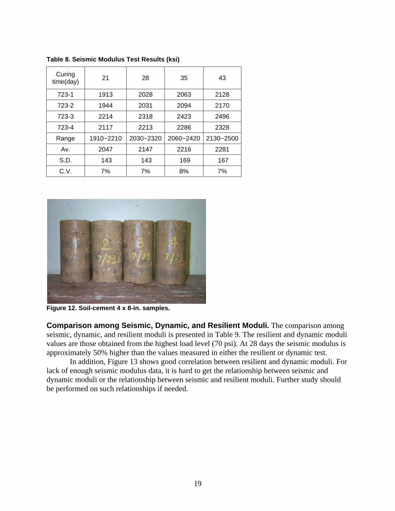
Figure 12. Soil-cement 4 x 8-in. samples. Comparison among Seismic, Dynamic, and Resilient Moduli. The comparison among seismic, dynamic, and resilient moduli is presented in Table 9. The resilient and dynamic moduli values are those obtained from the highest load level (70 psi). At 28 days the seismic modulus is approximately 50% higher than the values measured in either the resilient or dynamic test.

In addition, Figure 13 shows good correlation between resilient and dynamic moduli. For lack of enough seismic modulus data, it is hard to get the relationship between seismic and dynamic moduli or the relationship between seismic and resilient moduli. Further study should be performed on such relationships if needed.

20

Table 9. Comparison among Seismic, Dynamic, and Resilient Moduli

3-day 7-day 14-day 28-day

Modulus Range (ksi)

Seismic 2030~2320

Dynamic 1020~1200 1140~1500 1200~1520 1320~1700

Resilient 980~1120 1120~1250 830~1830 1040~1350

Seismic 2147 Average Modulus Dynamic 1087 1298 1409 1447

(ksi) Resilient 1060 1253 1280 1257

Coefficient of Variation (%)

Seismic 7

Dynamic 5 12 15 7

Resilient 7 9 29 10 Figure 13. Relationship between resilient and dynamic moduli.

As S-C is close to an elastic material, the results from the dynamic modulus and resilient

modulus should be very similar. The results after 7 days are 1298 and 1253 ksi, respectively. The differences observed are thought to do more with the measurement error in these low strain tests. The problems of running these tests will be discussed in the next chapter of this report.

Unconfined Compressive Strength (UCS). Only two of the six samples, 702-1 and 702-3, were broken on the 28th day. Table 10 shows the tabulated UCS results.

y = 1.462x - R2 =

0

500

1000

1500

2000

2500

3000

700 900 1100 1300 1500 1700 1900 2100 Dynamic Modulus (ksi)

Resilient Modulus(ksi)

21

Table 10. UCS Test Results

28-day UCS (psi) 702-1 599 702-3 395

Summary and Recommendations This report presents the repeatability test results of the seismic, dynamic, and resilient modulus tests. In addition, the results of UCS tests are discussed. Comparison of three modulus test methods is shown in Table 11.

Clearly the seismic modulus shows potential as it fairly inexpensive and a rapid test, but if the design program requires the use of resilient modulus values then a modulus correction factor must be developed. This will be explored in the next chapter of this report.

Table 11. Comparison of Three Modulus Test Methods

Seismic Modulus

Test

Dynamic Modulus

Test

Resilient Modulus

Test Equipment Cost $5000 $40,000 $350,000

Testing Time 3 minutes 40 minutes 30 minutes

Sample Capping No capping Capping Capping

Coefficient of Variation@28 day 7% 7% 10%

22

CHAPTER 3 CASE STUDY: DETERMINING INPUT VALUES FOR THE DESIGN GUIDE In determining input values for normal S-C and CMS materials the designer has two options:

• Conduct laboratory tests such as those described in Chapter 2 • Use standard regression equations developed to relate the required design properties

such as resilient modulus and modulus of rupture to known material properties (typically 7-day UCS)

A case study is presented in this chapter on how an agency can establish design

values for a typical stabilized base and soils material. In addition, the influence of different sample sizes is reported. The standard recommended procedure calls for a 2:1 height to diameter ratio, which for base materials typically required a 12 x 6-in. sample. Many agencies, including The Texas Department of Transportation (TxDOT) and PCA, would prefer to use smaller samples. Specimen Preparation Two materials were used for this evaluation. One was a typical limestone base obtained from Martin Marietta’s Beckman Pit in San Antonio, Texas, and the other was a typical sandy soil obtained locally through the Bryan TxDOT office. The results of a wet sieve analysis are given in Table 12 for the limestone base. The optimum moisture content of this material was found to be 6.2%. The optimum moisture content of the sandy soil was found to be 8.0%.

Table 12. Wet Sieve Analysis of Limestone Aggregate

Sieve Size Sieve Size (mm)

Retained Weight(g) % Retained % Passing

1 1/4-in. 31.750 0.0 0.0 100.0

7/8-in. 22.225 648.5 18.6 81.4

5/8-in. 15.875 580.0 16.6 64.8

3/8-in. 9.525 405.0 11.6 53.2

No. 4 4.750 404.4 11.6 41.6

No. 10 2.000 238.6 6.8 34.8

No. 40 0.425 206.0 5.9 28.9

No. 200 0.075 201.7 5.8 23.1

Pan Pan 806.6 23.1 0.0

This material is commonly used in the Districts in central Texas and the normal

cement content is 3%. This is based on achieving a 7-day UCS of 300 psi. Therefore, in the limestone base, 3% type I portland cement was used, and six samples each of 6 x 8-in. and 6 x 12-in. specimens were molded in the laboratory. As recommended by TxDOT procedures, the compaction moisture was determined by increasing the optimum moisture at a rate of

23

0.25% for each 1.0% cement added to the specimen. For sample preparation, the aggregates larger than ¾ in. were scalped. The 6 x 8-in. specimens were compacted using the TxDOT recommended four lifts of 50 blows each with a 10-lb hammer dropped from a height of 18 in. The 6 x 12-in. specimens were compacted using the modified Proctor in six lifts of 122 blows each with a 10-lb hammer dropped from a height of 18 in.

For testing of the sand material, based on the 7-day 300 psi UCS requirement, the researchers used 8% Type I portland cement. Six samples each of 4 x 8-in. and 4 x 4.5-in. specimens were molded in the laboratory. The compaction moisture was, again, determined by increasing the optimum moisture at a rate of 0.25% for each 1.0% of cement added to the specimen. The 4 x 8-in. specimens were compacted in six lifts of 25 blows each with a 10-lb hammer dropped from a height of 18 in. The 4 x 4.5-in. specimens were compacted in four lifts of 25 blows each with a 10-lb hammer dropped from a height of 18 in.

Three samples each of both the 3% S-C base and 8% cement treated sand were molded for the modulus of rupture test. These samples were 6 x 6 x 20 in. and were compacted in two lifts at 72 blows with a 10-lb tamper. Figure 14 shows the molded beam specimens.

Figure 14. Molded beam specimen for modulus of rupture.

After compaction, molded specimens were placed in the moisture room for curing.

Researchers conducted seismic modulus testing on each of the cylindrical samples at 1, 3, 7, 14, and 28 days. The resilient modulus and UCS tests were conducted at 7 and 28 days. The modulus of rupture was conducted after 28 days of curing. For each set of the cylindrical specimens molded in the lab, three were tested for seismic modulus, resilient modulus, and UCS through 7 days, while the other three were tested through 28 days of curing. Since the seismic and resilient modulus tests are nondestructive, the same samples could also be used for UCS. All samples were capped prior to testing for the resilient modulus and UCS testing.

Test Results and Discussion

Seismic Modulus. The free-free resonant column test shown in Figure 15, is a simple, nondestructive laboratory test for determining the modulus of pavement materials. The method was originally developed for testing portland cement concrete specimens, but with appropriate modifications in hardware and software it is now also applicable to specimens of base and subgrade materials.

24

Figure 15. Setup of free-free resonant column test.

The results of these can be seen in Tables 13-16 below. Results for this test are the

average of three different readings for each specimen tested with a less than ±10% variation among each reading. Table 13. Seismic Modulus Test Results for 6 x 8-in. Samples (ksi)

Curing time (day) 1 3 7 14 21 28

6x8A 1649.5 1951.6 6x8B 1444.6 1680.8 6x8C 1428.4 1629.1 6x8D 1348.9 1601.8 1774.5 1924.4 2012.9

6x8E 1191.2 1567.8 1929.0 2090.3

6x8F 1338.5 1535.0 1790.4 1963.2 2064.4 Table 14. Seismic Modulus Test Results for 6 x 12-in. Samples (ksi)

Curing time (day) 1 3 7 14 21 28

6x12A 1255.6 1695.2 2003.4 6x12B 1075.5 1630.9 2113.2 6x12C 1579.1 2016.3 2379.1 6x12D 1629.3 1749.0 2092.3 2366.4 2553.6 2612.6

6x12E 1706.8 1853.6 2219.6 2457.9 2648.3 2738.5

6x12F 1815.5 2040.7 2348.5 2648.5 2797.7 2920.0

25

Table 15. Seismic Modulus Test Results for 4 x 8-in. Samples (ksi)

Curing time (day) 1 2 5 7 21 28

4x8A 786.3 1303.4 1331.6

4x8B 750.4 1223.7 1260.0

4x8C 823.8 1294.0 1321.7

4x8D 1123.8 659.7

4x8E 418.0 1736.3

4x8F 874.1 1784.0 Table 16. Seismic Modulus Test Results for 4 x 4.5-in. Samples (ksi)

Curing time (day) 1 2 5 7 21 28

4x4.5A 0.1 0.1 0.6

4x4.5B 0.6 0.1 0.6

4x4.5C 0.1 0.1 0.6

4x4.5D 11.1 84.5 0.9 0.6

4x4.5E 6.0 31.6 0.4 105.6

4x4.5F 6.6 74.7 64.3

As can be seen from the data shown in Tables 13–16, there is an expected trend in the data, in that the seismic modulus increases with time. However, it can also be seen from the data in Table 16 that it was not possible to test the 4 x 4.5-in. samples. This is most likely due to the fact that these samples are far below the 2:1 length to diameter ratio as required for this test to allow for the necessary wave propagation for the testing software to calculate the seismic modulus. Samples for this test are recommended to be a minimum of 1.5:1 length to diameter ratio. In fact, resilient modulus testing was also not performed on these short samples, as there is a minimum of a 4-in. gage length required for that testing. Therefore, results for the 4 x 4.5-in. samples will not be considered. For this reason, these results will also be disregarded in any further analysis. The remaining data will be used to affirm the repeatability of the seismic modulus test as well as to validate the results of the resilient modulus test. It also appears that sample length does have an impact on the measured results. From Tables 13 and 14, it can be seen that the 8- and 12-in.-long samples provided different answers. The average seismic modulus at 7 days for the 8-in.-long sample was 1660 ksi and for the 12-in. sample was 2192 ksi. However, the interpretation is not clear as these samples were compacted differently. The standard TxDOT compactive effort was used for the 6 x 8 in. but higher modified for the 6 x 12-inch samples. Resilient Modulus. The standard test method used for resilient modulus testing was AASHTO DESIGNATION T 292-91. Measurements of the resilient modulus were taken after 7 days and 28 days of moist curing. These measurements were initially taken under a 50 psi loading level for the testing conducted at 7 days for the 6 x 8-in. S-C samples. However, these initial tests resulted in very little movement of the LVDTs due to the stiffness of the S-

26

C material; therefore, the loading level was increased 100 psi in future testing of both the 6 x 8-in. and the 6 x 12-in. samples. The loading level was set at 50 psi for the 4 x 8-in. cement modified sand specimens. These loads were applied cyclically for a 0.1 s of loading and 0.9 s of unloading to the unconfined specimen. The total resilient axial strain of each specimen after a 200-cycle conditioning period is measured with LVDTs, and the results from the last five cycles are used to calculate the resilient modulus.

Previous experience with the resilient modulus testing dictated that each specimen be plaster capped before the testing could be conducted to ensure that the tops of the samples were perpendicular to the sides. This is necessary because not doing so would result in unequal movement in the LVDTs, which would lead to unreliable results. Also, extreme care must be taken to ensure the proper placement of the LVDTs onto the sample. This step is time consuming and difficult due to the nature of the preparation procedure. In this part of the process, the LVDTs must be positioned 180° apart and perfectly parallel with the length of the sample. Figure 16 shows the preparation process.

27

16a) Plaster Cap on the Sample 16b) Leveling the LVDT Attachments

16c) Gluing LVDT Attachments to Sample 16d) Fastening LVDTs to Sample Figure 16. Sample preparation for the resilient modulus test.

Results for the resilient modulus test are shown in Tables 17-19.

Table 17. Resilient Modulus Test Results for 6 x 8-in. Samples (ksi)

Curing Days 7 28

6x8A 1615.7

6x8B 929.3

6x8C 1429.2

6x8D 1236.9

6x8E 987.2

6x8F 1449.7

28

Table 18. Resilient Modulus Test Results for 6 x 12-in. Samples (ksi)

Curing Days 7 28

6x12A 1263.2

6x12B 1401.9

6x12C 1827.7

6x12D 2010.7

6x12E 1904.7

6x12F 1947.6

Table 19. Resilient Modulus Test Results for 4 x 8-in. Samples (ksi)

Curing Days 7 28

4x8A 1258.0

4x8B 1306.0

4x8C 1302.0

4x8D 1435.1

4x8E 1467.8

4x8F 1450.2

Figures 17 and 18 show the movement in the LVDTs for Sample 6X8B at 7 days. The Y-axis designates displacement in inches, and the X-axis designates time in seconds. These data show some of the problems with running the resilient modulus test on very stiff materials. Results shown in Figure 18 are judged as reasonable. The movement of LVDT 8 for each load pulse can be clearly seen. However, the movement is very small at around 0.0003-in. The noise on the system is the scatter of data at the zero line. For this reasonable test the noise level is approximately 25% of the data level. The data from Figure 18 should be compared with that from LVDT 7 on the other side of the sample. The movement is much smaller and the actual data are largely masked by the noise on the channel. Even with extreme care taken in preparation of the samples, the movement in the LVDTs was not equal, and the results for this particular sample are questionable at best. This variation is explained by slight variations in the finishing of the sample, primarily that the ends are not precisely level. This is not a problem with normal granular materials where the seating loads will eliminate this effect. This clearly does not occur with cement stabilized materials. As was previously noted, the 6 x 8-in. samples that underwent resilient modulus testing at 7 days were tested at a loading level of 50 psi. All further testing of both 6 x 8-in. and 6 x 12-in. S-C samples was done under a 100 psi loading level.

29

0.0706

0.0708

2 2.5 3 3.5 4 4.5 5 5.5

Time (sec)

Dis

palc

emen

t

Figure 17. Displacement in LVDT 7 for Sample 6x8B at day 7.

0.0866

0.0872

2 2.5 3 3.5 4 4.5 5 5.5

Time (sec)

Dis

palc

emen

t

Figure 18. Displacement in LVDT 8 for Sample 6x8B at day 7.

30

Figures 19 and 20 show the movement in the LVDTs for Sample 6X12D at 7 days. As can be seen from these figures, movement was experienced in both LVDTs. However, LVDT 7 only experienced approximately 0.0002 in. of movement, while LVDT 8 underwent approximately 0.0003 in. This unequal movement further demonstrates the difficulty in accurately running this testing procedure. An average is taken between the two LVDTs to calculate the resilient modulus.

0.08395

0.0843

1 1.5 2 2.5 3 3.5 4 4.5

Time (sec)

Dis

palc

emen

t

Figure 19. Displacement in LVDT 7 for Sample 6x12D at day 7.

0.0864

0.0869

1 1.5 2 2.5 3 3.5 4 4.5

Time (sec)

Dis

palc

emen

t

Figure 20. Displacement in LVDT 8 for Sample 6x12D at day 7.

31

Table 20 gives the moduli taken from each LVDT individually and further demonstrates the variability inherent in this test method. Included in this table is a ratio of the results for LVDT 8 to LVDT 7.

Table 20. Resilient Modulus (ksi) for Each LVDT Sample LVDT 7 LVDT 8 Ratio (8:7)

6x8A 1615.08 1616.25 1.00

6x8B 3085.15 547.03 0.18

6x8C 1823.47 1175.10 0.64

6x8D 976.94 1685.54 1.73

6x8E 1133.29 874.47 0.77

6x8F 1380.21 1526.58 1.11

6x12A 1075.93 1529.36 1.42

6x12B 1354.13 1453.08 1.07

6x12C 2464.25 1452.51 0.59

6x12D 2272.56 1803.01 0.79

6x12E 2343.85 1604.20 0.68

6x12F 1868.52 2033.64 1.09

4x8A 886.62 2165.00 2.44

4x8B 1433.50 1199.41 0.84

4x8C 2608.16 867.55 0.33

4x8D 1188.55 1810.76 1.52

4x8E 1316.43 1658.59 1.26

4x8F 898.27 3761.66 4.19

In conclusion, the standard resilient modulus test is extremely difficult to run on typical S-C materials. Sample preparation and sensor mounting is difficult, and the equipment required is expensive. Compounding this is the signal to noise issue described above. It is seriously doubted that most Department of Transportation (DOTs) will ever run this test. They could potentially use seismic results or most probably rely on relationships with UCS tests. Unconfined Compressive Strength (UCS). UCS is the most widely used test to evaluate cement stabilized material strength. ASTM D1633 was the standard test method used to measure the UCS of the samples; however, the samples were not immersed in water for 4 hours. The load is applied continuously and without shock at an approximate rate of 0.135 in./min.

All samples were tested for UCS. Of the six samples compacted for each mix design, three were tested at 7 days, and three were tested at 28 days. Results for this testing are shown below in Table 21.

32

Table 21. UCS Test Results 7-day UCS (psi) 28-day UCS (psi)

6x8A 682.8 6x8B 522.6 6x8C 628.8 6x8D 790.4 6x8E 579.9 6x8F 757.8

6x12A 447.9 6x12B 690.8 6x12C 674.4 6x12D 990.87 6x12E 997.74 6x12F 1190.28 4x8A 342.5 4x8B 399.3 4x8C 374.6 4x8D 392.0 4x8E 561.2 4x8F 456.7

Modulus of Rupture (Mrup). Three samples each of 3% S-C base and 8% cement-treated sand were prepared for testing to determine the modulus of rupture. All were tested after 28 days of moist-curing and were tested using the Simple Beam with the Third-Point Loading method. A schematic of the test setup is shown in Figure 21.

Figure 21. Third-point loading of a simple beam.

Results for this testing are shown in Table 22. Samples designated as “CTB” were the S-C base, and samples designated with “CTS” were the cement-treated sand. It should be

33

noted that sample CTB-B broke prior to being tested, so these results will be disregarded in any further analysis. This test is for concrete beams, and it is very difficult to conduct on S-C bases and cement modified materials, which have substantially lower early strengths. As discussed for the resilient modulus it is doubtful that this test will be run for routine design by DOTs. Table 22. Modulus of Rupture

Sample 28-day Mrup (psi) CTB-A 155.1 CTB-B* 6.4 CTB-C 187.9 CTS-A 132.0 CTS-B 109.0 CTS-C 109.0

*Sample broken prior to testing. Relationships between Testing Procedures Seismic and Resilient Moduli Tests. A comparison of the resilient and seismic moduli was done in order to validate the use of the seismic modulus testing in performance-based design of pavement layers. Previous research performed by Nazarian and Yuan (2004) laid the foundation for the relationships between the low-strain resilient modulus and seismic modulus for granular materials, in which the following relationship was established:

Mr = 0.5516* MS (12) where

Mr = resilient modulus and MS = seismic modulus

For this portion of the research, results for the cement modified samples with a 2 to 1 length to diameter ratio were used for comparison, which is the recommended sample size for these tests. This means that the results for the 6 x 12-in. S-C base samples and the 4 x 8-in. CMS samples were used. Figure 22 shows the relationship that was established for these materials, which is:

Mr = 0.45358MS + 642.92 (13)

Removing the intercept value, the following relationship was found:

Mr = 0.749 * MS (14)

Given the time-consuming and tedious nature of the test setup for the standard resilient modulus test, and the difficulty with sensor mounting and signal to noise ratio that was previously discussed, it is doubtful that this test will be run on a routine basis. Figure 22 illustrates the potential of using the seismic modulus test to obtain the required resilient modulus value.

34

y = 0.4535x + 642.92R2 = 0.7979

0.0

500.0

1000.0

1500.0

2000.0

2500.0

0.0 500.0 1000.0 1500.0 2000.0 2500.0 3000.0 3500.0

Seismic Modulus (ksi)

Res

ilien

t Mod

ulus

(ksi

)

2:1 Linear (2:1) Figure 22. Comparison of low-strain resilient modulus to seismic modulus.

Unconfined Compressive Strength and Resilient Moduli Tests. A comparison of the UCS results to the resilient moduli was done in order to evaluate the use of the UCS testing to estimate the resilient modulus. Results for samples with a 2 to 1 length to diameter ratio were used for comparison, which is to say that the results for the 6 x 12-in. S-C base samples and the 4 x 8-in. CMS samples were used. Figure 23 shows the relationship that was established for these materials. The equation is:

Mr = 62.5 UCS (15)

where Mr is the Resilient Modulus (ksi)

UCS is the unconfined compressive strength (psi)

35

1000.0

1200.0

1400.0

1600.0

1800.0

2000.0

2200.0

10.0 15.0 20.0 25.0 30.0 35.0 40.0

Root UCS(psi)

Res

ilien

t Mod

ulus

4x8 CMS 6x12 S-C Base

Mr = 62.5*Root (UCS)R2 = 0.75

Figure 23. Comparison of resilient modulus to UCS. Modulus of Rupture and Unconfined Compressive Strength. There are several well-known relationships that have been established between the modulus of rupture (Mrup) at 28 days and UCS (psi) of concrete at 28 days. Two of these are those set forth by ACI and USACE and were previously shown as:

Mrup = 7.5 UCS and Mrup = 9.0459 UCS , respectively. where

Mr is Modulus of Rupture (psi) Figure 24 shows the relationship found for the S-C base and sand samples tested for UCS at 28 days and modulus of rupture at 28 days to be:

Mrup = 5.2851 UCS (16)

36

y = 5.2851xR2 = 0.9469

0.0

20.0

40.0

60.0

80.0

100.0

120.0

140.0

160.0

180.0

200.0

0.0 5.0 10.0 15.0 20.0 25.0 30.0 35.0 40.0

Sqrt UCS (psi)

Mod

ulus

of R

uptu

re (p

si)

Figure 24. Comparison of modulus of rupture to 28-day UCS. Figure 24 indicates that there is generally a strong relationship between modulus of rupture and UCS. Given that the relationships established by ACI and the USACE were for the UCS of concrete at 28 days, it is reasonable to assume that the UCS of a S-C base or sand with the same curing time would be lower. To be of use to pavement designers it will be necessary to develop relationships between the 7-day UCS and the design parameter modulus of rupture at 28 days. The 7-day UCS is widely used in specifications for S-C bases. From the data presented in Tables 21 and 22, excluding the results for the B sample, the following relationships were developed. From the limited data set for S-C bases; 7rup UCS24.7M = (17) From the limited data set for CMS; 7rup UCS04.6M = (18) where

Mrup is the modulus of rupture after 28 days, and UCS7 is the unconfined compressive strength after 7 days moist cure.

Summary From the results presented in this chapter, determining the resilient modulus using traditional test procedures in the laboratory will be very problematic for most DOTs. The test equipment is expensive, and the test procedures are very difficult to run. The existing test procedures have been developed from granular/lower stiffness materials. When using stiff materials, it is critical to cap the samples. Even with very good control, as was used in this test program,

37

problems were encountered with the different displacement sensors reading completely different strain levels. It is very difficult to imagine how most DOTs will handle the level 1 (lab test) requirement for the mechanistic empirical design procedures.

The seismic modulus test appears to offer a feasible alternative. The drawback of this test is that it does appear to be sensitive to sample dimensions. The need for a 2:1 height to diameter ratio is standard but as found in Tables 13 and 14 there is a significant difference in results from 6 x 12- and 6 x 8-in. samples. It appears that for base materials the 6 x 12-in. samples are recommended. From the results obtained, the resilient modulus is 75% of that measured in the seismic test on the 6 x 12-in. samples. Given that the seismic modulus equipment is less than $5,000, this offers a realistic alternative to running the traditional test procedures. The relationships between UCS and the resilient modulus are based on a very limited data set, but is somewhat similar to those recommended by other agencies. Recommendations on values to use in the software developed in this study will be provided in the summary of this report.

38

CHAPTER 4 MODULI MEASUREMENTS IN THE FIELD Several test systems have long been used to evaluate the structural capacity of in situ pavements. Some devices measure deflections and backcalculate the elastic moduli of various pavement components. Other nondestructive testing methods involve the use of wave propagation, impact hammer, and impedance devices. A summary of the most popular devices and examples of how they can be used to measure field resilient modulus will be described in this chapter. Falling Weight Deflectometer (FWD) Description of FWD. The FWD shown in Figure 25 is the most popular nondestructive testing device used to structurally test pavements during rehabilitation studies, research, and pavement structural failure investigations. It is used for conventional and deep strength flexible, composite, and rigid pavement structures.

The FWD is a device capable of applying impulse loads to the pavement surface, similar in magnitude and duration to that of a single heavy moving wheel load. The response of the pavement system is measured in terms of vertical deformation, or deflection, over a given area using geophones. The FWD measures a deflection basin caused by a controlled load. These results make it possible to treat pavement structures in the same manner as other civil engineering structures by using mechanistically based design methods. FWD generated deflection basins, combined with layer thickness, can be used to calculate the "in situ" resilient elastic moduli of a pavement structure, using a process known as backcalculation. This information can also be used in structural analysis to determine the bearing capacity, estimate remaining life, and calculate overlay requirements over a desired design life.

Figure 25. Falling weight deflectometer. Moduli Backcalculation from FWD Data. One of the most useful applications of FWD testing is to backcalculate the moduli of pavement components including the subgrade. The basic procedure is to measure the pavement deflection basin normally with seven sensors at different offsets from a load plate. Then using the design layer thicknesses, a mathematic model (typically a linear-elastic program) is run numerous times, varying the moduli value of each layer. The process is stopped when an acceptable match is obtained between the

39

theoretically calculated and measured deflection bowls. A variety of methods based on layer elastic theory have been developed to backcalculate layer moduli.

Modulus 6.0 is one of the well-known backcalculation procedures. This computer program was developed by the TTI for TxDOT for backcalculating layer moduli (Liu and Scullion 2002). As shown in Figure 26, it can be applied to a two-, three-, or four-layer system with or without a rigid bedrock layer. For each layer in the pavement structure the user provides a range of moduli values. A linear elastic program is run to generate a database of calculated deflection bowls by assuming a number of different moduli values within the supplied range. Once the database is developed, a pattern search routine is used to match each of the field measured deflection bowls with theoretical bowls within the database.

Figure 26. Moduli calculation screen in modulus software.

To demonstrate, use the FWD to determine the moduli value for a S-C base. FWD data was collected on a section of US 290 in the Bryan District immediately after placement but prior to placing the asphalt surface. Deflection data was also collected in 2005 after the pavement had been in service for 3 years.

The original S-C base was the same material as that tested in Chapter 3 of this report. In the laboratory, samples were compacted at 3% cement; however, in this field operation the target cement content was 3.5%. The FWD data was collected directly on top of the treated base. The Modulus 6.0 output for that base is shown in Table 23. The S-C base at the time of testing ranged from 3 to 45 days old. The base did not have significant traffic on it during that period, other than regular construction traffic. Based on the construction diaries, it was possible to find the age of the base at the time of the FWD data collection. For example, in Table 23 for the first two deflection bowls the base was 3 days old. The next 11 bowls (0.199 miles to 1.223 miles) the base was 45 days old. The average modulus was computed for each age of base, and the average results are shown in Figure 27. A very good linear relationship showing a rapid increase in field modulus with time was found for this data set. It is interesting to note that the field modulus is approximately 50% of that measured in the laboratory. From Table 18, the resilient modulus measured in the lab after 28 days was 1953 ksi, whereas in the field the equivalent average moduli value was close to 1000 ksi. Clearly there are many differences between moduli values obtained from laboratory molded and cured samples and those obtained in the field.

40

The pavement received a 6-in. asphalt overlay and was opened to traffic for 3 years before it was retested. A core from the completed section is shown in Figure 28. A total of 6 in. of HMA surface was placed, and after 3 years no problems were detected in either layer. The backcalculated moduli value after 3 years is shown in Table 24. After 3 years in service the average backcalculated moduli value was close to 500 ksi, which is still high given that the moduli value routinely used for granular base layers in Texas is 50 ksi. Still, the issue remains as to what resilient modulus value to use for design. In this study the lab testing indicated a resilient modulus value of 2000 ksi was appropriate after 28 days. In the field before placement of the surface layer, average values close to 1000 ksi were calculated. After 3 years in service, the long-term average modulus for this layer was calculated to be close to 500 ksi. FWD data was also collected after year 2, and an average value of 500 ksi was also obtained.

This variation between moduli values determined in the laboratory and field is a well-known concept. The values obtained in the laboratory under ideal conditions will be substantially higher than those measured in the field. Which value to use for structural design is one of the major challenges with implementation of any mechanistic pavement design program. However every mechanistic-empirical design procedure requires calibration where predictions are matched with field performance. Clearly, in the calibration effort a decision is made as to which moduli value to use; that same moduli (lab or field determined) should be used in all future designs. With the new MEPDG, for the asphalt surface layers the moduli values recommended will be those computed in the lab using the dynamic modulus test. For the base layers, designers are given the option of using either laboratory or field determined values. From the discussion presented above for S-C bases, the range of values is very large, 500 to 2000 ksi. This will have a major impact on the resulting pavement design. The authors of this report suggest that the long-term field moduli values should be the conservative values to use for routine design.

Table 23. FWD Data Collected Shortly after Placement of S-C base ---------------------------------------------------------------------------------------------------------------------------------------- Load Measured Deflection (mils): Calculated Moduli values (ksi): Absolute Dpth to Station (lbs) R1 R2 R3 R4 R5 R6 R7 SURF(E1) BASE(E2) SUBB(E3) SUBG(E4) ERR/Sens Bedrock ---------------------------------------------------------------------------------------------------------------------------------------- 0.113 9,108 6.46 4.27 2.87 2.07 1.49 1.04 0.74 389.7 0.0 0.0 30.2 1.37 98.7 0.135 8,699 10.43 5.62 3.38 2.09 1.36 0.94 0.69 153.2 0.0 0.0 28.4 3.73 99.3 0.199 8,659 3.50 2.96 2.34 1.95 1.58 1.23 0.96 1593.3 0.0 0.0 25.9 1.20 116.1 0.301 8,588 4.48 3.81 3.07 2.58 2.07 1.65 1.34 1310.8 0.0 0.0 19.1 0.88 155.9 0.400 8,766 2.22 1.93 1.38 1.07 0.74 0.63 0.44 1707.5 0.0 0.0 52.4 4.37 97.1 0.500 8,544 3.75 3.36 2.73 2.35 1.91 1.46 1.13 1734.8 0.0 0.0 20.2 2.37 111.6 0.600 8,361 2.93 2.61 2.01 1.65 1.35 1.02 0.93 1783.6 0.0 0.0 29.5 2.52 117.3 0.701 8,226 2.70 2.33 1.70 1.35 1.06 0.78 0.66 1483.0 0.0 0.0 37.9 2.81 103.1 0.802 8,055 2.52 2.39 1.67 1.27 0.97 0.73 0.56 1469.4 0.0 0.0 39.0 4.86 110.4 0.927 8,218 3.96 3.30 2.40 1.87 1.39 1.03 0.83 894.8 0.0 0.0 28.2 2.54 117.8 1.027 8,119 3.60 2.75 2.04 1.64 1.31 1.03 0.82 1086.2 0.0 0.0 30.6 3.01 131.0 1.134 8,024 2.54 2.22 1.75 1.51 1.24 0.98 0.81 2326.5 0.0 0.0 29.7 1.58 137.3 1.234 8,369 2.17 1.52 1.15 0.98 0.84 0.67 0.53 2136.7 0.0 0.0 51.7 7.15 100.8 1.343 8,290 2.81 2.26 1.67 1.32 1.08 0.85 0.71 1487.6 0.0 0.0 37.8 3.13 149.6 1.461 8,178 3.63 2.94 2.13 1.64 1.25 0.95 0.77 965.3 0.0 0.0 31.4 1.94 132.7 1.567 7,952 4.79 4.07 3.20 2.59 2.00 1.52 1.19 927.9 0.0 0.0 18.9 1.78 137.0 1.681 8,016 5.38 4.39 3.18 2.42 1.81 1.34 1.08 616.2 0.0 0.0 21.1 2.28 129.9 1.770 8,333 3.67 3.09 2.38 1.95 1.52 1.14 0.93 1244.3 0.0 0.0 26.4 1.95 118.4 1.880 8,238 6.00 4.75 3.57 2.88 2.24 1.69 1.33 664.9 0.0 0.0 18.0 1.28 139.6 1.980 8,051 4.95 4.20 3.11 2.56 1.95 1.48 1.18 831.3 0.0 0.0 19.8 2.37 135.7 2.055 7,944 4.46 3.85 2.89 2.31 1.71 1.29 1.06 867.4 0.0 0.0 21.9 3.03 134.3 2.157 8,111 4.87 3.40 2.41 1.76 1.25 0.94 0.80 530.9 0.0 0.0 31.3 1.25 135.8 2.257 7,936 5.46 4.22 2.93 2.18 1.61 1.19 0.93 518.8 0.0 0.0 23.9 2.17 128.2 2.358 8,111 4.09 3.75 2.85 2.24 1.69 1.25 0.96 1028.0 0.0 0.0 22.5 4.47 122.0 2.448 7,658 7.45 5.65 4.07 3.08 2.25 1.70 1.37 386.1 0.0 0.0 16.4 1.48 161.0 2.547 8,071 4.22 3.59 2.78 2.22 1.75 1.32 1.07 1042.9 0.0 0.0 22.2 1.69 132.9 2.649 8,194 4.02 3.36 2.62 2.13 1.74 1.37 1.09 1232.2 0.0 0.0 22.6 1.75 138.8 2.732 7,920 7.25 5.69 3.96 2.84 2.01 1.46 1.18 365.1 0.0 0.0 18.6 3.74 130.3 2.835 7,881 5.47 4.35 3.21 2.40 1.69 1.15 0.85 532.2 0.0 0.0 22.3 4.66 94.7 2.961 7,924 5.37 4.59 3.27 2.42 1.76 1.31 1.06 585.8 0.0 0.0 20.9 4.07 138.6 3.060 8,063 4.46 3.72 2.78 2.20 1.70 1.32 1.09 893.9 0.0 0.0 22.7 1.81 162.5 3.145 7,980 5.53 4.24 3.12 2.52 1.94 1.54 1.28 668.8 0.0 0.0 20.0 2.36 197.8 3.245 7,841 3.95 2.96 2.11 1.62 1.17 0.82 0.63 710.1 0.0 0.0 33.0 2.27 93.5 3.301 7,881 7.86 6.07 4.23 3.07 2.24 1.59 1.28 340.5 0.0 0.0 17.1 2.75 117.8 3.401 7,730 7.00 5.62 4.47 3.67 2.94 2.31 1.92 655.5 0.0 0.0 12.6 1.18 208.5 3.504 8,024 4.51 3.44 2.46 1.90 1.38 1.02 0.84 673.4 0.0 0.0 28.1 1.72 118.6 3.614 7,789 5.00 3.26 2.30 1.75 1.27 0.96 0.80 493.6 0.0 0.0 30.7 2.79 134.4 3.718 7,531 9.84 7.04 4.74 3.43 2.55 1.88 1.59 238.0 0.0 0.0 14.6 2.40 147.3 3.812 7,730 7.53 6.04 4.41 3.32 2.49 1.87 1.52 419.7 0.0 0.0 14.8 1.90 159.3 3.922 7,730 6.87 5.37 3.83 2.83 2.02 1.45 1.15 400.7 0.0 0.0 18.3 2.98 120.5 4.028 7,722 7.82 4.90 3.35 2.55 1.91 1.45 1.21 295.1 0.0 0.0 20.7 4.39 153.4 ---------------------------------------------------------------------------------------------------------------------------------------- Mean: 5.01 3.90 2.84 2.20 1.66 1.25 1.01 919.2 0.0 0.0 25.6 2.63 125.5 Std. Dev: 1.97 1.27 0.87 0.64 0.48 0.36 0.31 539.3 0.0 0.0 8.9 1.28 22.1 Var Coeff(%): 39.3 32.6 30.5 28.9 28.7 28.9 30.2 58.7 0.0 0.0 34.7 48.5 17.6

41

42

C h a n g e in S -C b a s e m o d u lu s w ith tim eU S 2 9 0 T e x a s

02 0 04 0 06 0 08 0 0

1 0 0 01 2 0 01 4 0 01 6 0 01 8 0 0

0 1 0 2 0 3 0 4 0 5 0

D a y s s in c e p la c e m e n t

Mod

ulus

(ksi

)

Figure 27. Summary of gain of modulus with time.

Figure 28. Core from the test pavement after 3 years in service.

Table 24. FWD Data Collected after 3 Years in Service District: Bryan MODULI RANGE(psi) County : Burleson Thickness(in) Minimum Maximum Poisson Ratio Values Highway/Road: US 290 Pavement: 6.00 600,000 1,500,000 H1: v = 0.35 Base: 14.00 150,000 1,500,000 H2: v = 0.20 Subbase: 0.00 H3: v = 0.00 Subgrade: 119.14(User Input) 20,000 H4: v = 0.40 ---------------------------------------------------------------------------------------------------------------------------------------- Load Measured Deflection (mils): Calculated Moduli values (ksi): Absolute Dpth to Station (lbs) R1 R2 R3 R4 R5 R6 R7 SURF(E1) BASE(E2) SUBB(E3) SUBG(E4) ERR/Sens Bedrock ---------------------------------------------------------------------------------------------------------------------------------------- 0.000 9,688 4.26 3.44 2.72 2.19 1.85 1.48 1.32 1500.0 470.9 0.0 14.9 2.14 175.0 * 0.100 9,259 4.75 3.85 3.15 2.56 2.07 1.59 1.27 1499.9 362.3 0.0 12.7 0.48 123.1 * 0.200 9,493 3.31 2.60 2.09 1.61 1.19 0.89 0.70 1500.0 463.2 0.0 24.0 2.58 98.8 * 0.300 9,446 2.70 2.00 1.65 1.39 1.15 0.89 0.72 921.1 1429.5 0.0 23.4 0.92 101.3 0.400 9,168 3.52 2.91 2.40 1.99 1.61 1.22 0.98 1500.0 616.5 0.0 15.7 1.67 101.9 * 0.600 9,311 4.00 3.50 2.98 2.52 2.14 1.74 1.51 1500.0 771.3 0.0 10.3 1.22 300.0 * 0.700 9,255 4.98 4.04 3.26 2.65 2.23 1.83 1.56 1170.3 436.1 0.0 11.3 1.85 300.0 0.800 9,072 6.56 4.59 3.33 2.62 2.09 1.63 1.31 600.0 223.6 0.0 14.2 3.64 135.4 * 0.900 9,255 3.84 3.26 2.76 2.20 1.81 1.37 1.10 1500.0 561.2 0.0 13.8 2.37 110.9 * 1.000 9,203 4.28 3.54 2.79 2.19 1.75 1.33 1.13 1500.0 333.3 0.0 15.9 1.47 114.9 * 1.100 9,235 3.44 2.65 2.20 1.80 1.49 1.17 1.01 1082.5 788.3 0.0 17.5 0.70 130.3 1.200 9,124 3.87 3.10 2.47 1.88 1.38 1.05 0.88 1500.0 334.0 0.0 19.7 2.53 116.3 * 1.300 9,092 3.03 2.41 2.04 1.72 1.44 1.16 1.02 1323.6 1042.6 0.0 16.5 0.57 300.0 1.400 9,183 3.61 2.97 2.40 1.93 1.54 1.18 0.94 1500.0 517.3 0.0 17.0 1.28 113.1 * 1.500 9,064 7.37 5.44 3.75 2.86 2.24 1.73 1.44 607.1 159.8 0.0 13.3 3.53 143.1 1.600 9,084 4.04 3.37 2.81 2.27 1.88 1.43 1.30 1500.0 490.6 0.0 13.3 1.62 113.2 * 1.700 9,100 4.07 3.23 2.67 2.17 1.77 1.37 1.19 1377.4 484.9 0.0 14.5 0.44 124.8 1.800 9,195 3.98 3.51 3.06 2.62 2.23 1.76 1.53 1500.0 779.9 0.0 9.8 2.08 141.7 * 1.901 9,104 4.03 3.44 2.97 2.35 1.89 1.52 1.38 1500.0 531.1 0.0 12.4 2.25 300.0 * 2.000 9,052 5.08 4.12 3.14 2.50 2.00 1.57 1.37 1500.0 258.2 0.0 13.5 1.58 152.1 * 2.100 9,076 3.96 2.88 2.30 1.83 1.48 1.14 0.97 701.3 613.4 0.0 18.7 1.24 118.1 2.200 8,977 4.37 3.75 2.99 2.35 1.89 1.45 1.22 1500.0 336.7 0.0 13.9 1.82 125.9 * 2.300 9,048 4.55 3.98 3.15 2.52 2.04 1.59 1.31 1500.0 370.5 0.0 12.3 1.94 141.5 * 2.400 9,017 5.11 4.24 3.43 2.80 2.26 1.74 1.48 1500.0 315.0 0.0 11.2 0.68 128.4 * 2.500 9,100 4.50 3.80 3.16 2.63 2.18 1.69 1.44 1500.0 465.3 0.0 11.1 1.10 128.1 * 2.800 9,104 4.42 3.61 2.89 2.27 1.79 1.34 1.08 1500.0 311.6 0.0 15.4 1.37 107.0 * 2.900 9,116 4.35 3.68 3.08 2.50 2.03 1.57 1.30 1500.0 454.5 0.0 12.1 1.53 130.1 * 3.101 9,025 4.13 3.30 2.67 2.20 1.82 1.45 1.28 1289.5 511.7 0.0 13.8 1.18 162.4 3.200 9,052 3.99 3.02 2.42 1.94 1.53 1.15 0.94 1081.7 451.0 0.0 18.0 0.40 102.3 3.300 9,048 3.93 3.35 2.82 2.38 2.01 1.63 1.43 1500.0 695.3 0.0 11.1 0.80 300.0 * 3.400 9,052 6.35 5.19 4.15 3.26 2.61 2.02 1.75 1478.1 197.8 0.0 10.2 0.53 151.6 3.500 9,156 4.11 3.21 2.56 2.08 1.65 1.28 1.11 1317.0 426.6 0.0 16.3 0.42 124.4 3.600 9,056 4.02 3.08 2.38 1.86 1.51 1.17 1.03 1175.1 407.4 0.0 18.4 1.72 126.8 3.700 9,029 5.88 4.67 3.69 3.00 2.46 1.97 1.69 895.3 324.2 0.0 10.5 1.59 300.0 3.801 8,909 5.83 4.62 3.52 2.74 2.18 1.70 1.46 1122.3 220.5 0.0 12.5 1.48 154.6 3.900 8,901 3.96 3.38 2.79 2.31 1.93 1.52 1.31 1500.0 569.6 0.0 12.0 1.26 144.0 * 3.975 8,953 4.72 3.80 3.07 2.56 2.14 1.69 1.46 1100.3 469.1 0.0 11.6 1.28 150.9 --------------------------------------------------------------------------------------------------------------------------------------- Mean: 4.40 3.55 2.86 2.30 1.87 1.46 1.24 1317.4 491.8 0.0 14.4 1.49 139.1 Std. Dev: 0.97 0.73 0.51 0.40 0.34 0.28 0.25 274.0 243.3 0.0 3.5 0.79 38.6

43

44

Portable Seismic Pavement Analyzer (PSPA) The PSPA, as shown in Figure 29, is an instrument designed to determine the variation in modulus with depth for pavement systems. The operating principle of the PSPA is based on generating and detecting stress waves in a medium. The PSPA consists of two transducers and a source packaged into a hand-portable system, which can perform the Ultrasonic Surface Wave (USW) and Impact Echo tests (Nazarian et al. 2005). The USW method can be used to determine the modulus of the material. The Impact Echo method can be used as a tool to determine the thickness or the bonding condition of concrete slabs.

The PSPA is operable from a computer. This computer is tethered to the hand-carried transducer unit through a cable that carries power to the transducers and hammers and returns the measured signals to the data acquisition board in the computer. To collect data with the PSPA, the technician initiates the testing sequence through the computer. The high-frequency source is activated four to six times. The outputs of the two transducers from the last three impacts are saved and averaged (stacked). The other (pre-recording) impacts are used to adjust the gains of the pre-amplifiers. The gains are set in a manner that optimizes the dynamic range.

Typical voltage outputs of the two accelerometers are shown in Figure 30. To ensure that an adequate signal to noise ratio is achieved in all channels, signals are normalized to a maximum amplitude of one. In this manner, the main features of the signals can be easily inspected.

Connecting Cable

LaptopPSPA

Connecting Cable

LaptopPSPA

Source

Receiver A

Data Acquisition

Box

Receiver B

Source

Receiver A

Data Acquisition

Box

Receiver B

Figure 29. Portable seismic pavement analyzer (Nazarian 2006).

45

0.2 0.4 0.6 0.80.0 1.0

Nor

mal

ized

Am

plitu

deNear Accelerometer

Time, msec

Far Accelerometer

0.2 0.4 0.6 0.80.0 1.0

Nor

mal

ized

Am

plitu

deNear Accelerometer

Time, msec

Far Accelerometer

Figure 30. Typical timer records from PSPA (Nazarian, 2006).

The data, collected in this fashion, have to be processed using signal processing and spectral analyses (Nazarian 2003). The basics of the analysis are based on the following relationship between velocity, V; travel time, Δt; and receiver spacing, ΔX:

tX = VΔΔ (19)

In the equation, V can be the propagation velocity of any of the three waves [i.e.,

compression wave, VP; shear wave, VS; or surface (Rayleigh) wave, VR]. Knowing wave velocity, the modulus can be determined in several ways. Young's modulus, E, can be determined from shear modulus, G, through the Poisson's ratio, ν, using:

E = 2 (1+ν) G (20) Shear modulus can be determined from shear wave velocity, VS, using:

2sV

g =G γ (21)

To obtain the modulus from surface wave velocity, VR is first converted to shear wave velocity using:

VS = VR (1.13-0.16ν) (22)

The shear modulus is then determined by using Equation 21. Using techniques described elsewhere (Nazarian 2003), it is possible to measure the phase velocity of different wavelengths of seismic waves as shown in Figure 31. As shown this can be related to the various layers within the pavement structure so it is possible to obtain a seismic modulus for each layer in the pavement structure.

46

Figure 31. Schematic of USW method. The PSPA is currently being used by TxDOT to test the uniformity of pavements being

constructed with S-C bases (Nazarian 2006). The PSPA setup in the field is shown in Figure 32. The unit is self contained with a laptop computer to collect and interpret data.

Figure 32. PSPA used to collect seismic modulus of S-C layers in the field. The one advantage of the seismic modulus test is that samples can also be measured in the laboratory with the free-free resonant column test described in Chapter 2 and then measured in the field with the PSPA. Data from a recent test on a section of Interstate Highway 20 in the Odessa District are shown in Figure 33. The laboratory value is given as the green line with a measured value of close to 600 ksi. The results from the field are highly variable. This is ongoing work (Nazarian 2006) and full details will be provided to the project sponsors in the near future. However, this example does illustrate that seismic technology could also be used for quality control applications on S-C bases.

Source

Receiver AReceiver B

0

1

2

3

4

5

6

7

8

3000 3200 3400 3600 3800 4000Phase Velocity (ft/s)

Wav

elen

gth

(in.)

hDispersion Curve

VR1

VR2

(VR1)

Pavement Layout

(VR2)

47

Figure 33. Field data collected with the PSPA on a S-C base near Odessa, Texas (Nazarian 2006). Prima 100 As shown in Figure 34, the Prima 100 is a portable FWD. One operator can quickly measure the deflection of the soil layer and compute a composite layer stiffness. PRIMA 100 measures the force and deflection when a weight drops to the ground from an optional height. The reaction of the soil from this impulse is collected by up to three sensors and transferred to a personal computer where a computer program calculates the bearing capacity and modulus. The analysis uses a single layer Bousinesseq solution where a composite modulus is calculated for the entire pavement structure. Therefore, the results obtained are dependent on both base and subgrade stiffness. The current version of the Prima software does not do a layered analysis as performed with the FWD data.

0

200

400

600

800

1000

1200

0.0 0.5 1.0 1.5 2.0 2.5 3.0 3.5 4.0 4.5

Distance, mi

Mod

ulus

, ksi

Station AverageSection AverageSection STDLab-Cured Specimens with 3% Cement

48

Figure 34. Prima 100.

The system comes with two plate sizes, 8-in. and 12-in. diameter. The smaller plate

shown in Figure 34 puts a higher stress on the pavement and is recommended for stiff S-C layers. Sebesta (2004) conducted both Prima and FWD testing on a range of S-C base projects in Texas. This was part of a microcracking study where data were collected early in the life of the stabilized base, both before and after microcracking. Figure 35 shows the results of these studies.

y = 0.137x1.69

R2 = 0.7516

0

500

1000

1500

2000

2500

3000

3500

4000

0 50 100 150 200 250 300 350 400 450

PFWD E (ksi)

TxD

OT

FW

D (k

si)

Figure 35. Comparing base moduli from the FWD and Prima.

49

The Prima results were obtained with one sensor field unit, and they represent a composite modulus, which is dependent on both the base and subgrade stiffness. On the other hand, the FWD moduli is a computed number for the S-C layer only. As observed in Figure 35, the composite Prima and FWD (PFWD) modulus is substantially less than that computed from the FWD.

The PFWD could be a valuable tool for both S-C quality assurance testing and moduli determination but the data interpretation program will need to be improved. This can be done with the move to the three channel unit shown in Figure 34. The data should be included into a simple backcalculation system where two moduli values are developed, one for the upper S-C layer and one for the lower subbase. Preliminary development work in this area has been done at TTI, and the results look reasonable. The manufacturers of these devices are actively seeking to improve their software. Dynamic Cone Penetrometer (DCP)

The DCP is shown in Figure 36. The test consists of hand driving a standard cone through pavement layers with a 17.6 lb weight, which drops through 39 in. The average rate of penetration through various pavement layers is measured and used to estimate its in situ shear strength.

Figure 36. DCP testing device.

The DCP was originally designed and used for determining the strength profile of flexible

pavement structures. It can penetrate soil layers having California Bearing Ratio (CBR) strengths in excess of 100 and also measure soil strength less than 1 CBR. The DCP is easily used in the

50

field. An access hole is drilled through the upper layers and testing initiates at the layer of interest. Numerous studies have been conducted relating the DCP penetration rate to materials properties. The equation below is one typical relationship found in the literature:

*1.12*/292 DCPCBR = (23)

where DCP is the penetration ratio in millimeters per blow for the 17.6-lb hammer.

Although widely used in many subbase evaluations, application of the DCP to pavement

containing S-C or CMS layers is very limited because of the stiffness of the layers. These typically are too strong to test with the DCP. The DCP, however, is often used in the case of forensic investigation when durability problems are suspected with treated soil layers. However, this is rarely the case with CMS.

51

CHAPTER 5 A MECHANISTIC EMPIRICAL THICKNESS DESIGN PROGRAM FOR PAVEMENTS WITH S-C BASES OR CEMENT MODIFIED SOILS In this chapter a new mechanistic-empirical design program (CTB) is proposed for thickness design of pavements containing either S-C base or CMS layers. The inputs and design models of the new design program will be compared and contrasted with those proposed in the NCHRP/AASHTO Design Guide, or MEPDG. Also included will be a description of efforts made to provide calibration factors for the new CTB program as well as a user’s manual. In addition to CTB, a second program called CTBana was also developed to serve as a training tool for designers. Both programs use the same models and performance prediction equations but the CTB program provides substantially more options, particularly in the traffic input area. Background Two types of structural sections with S-C layers are proposed in the new Design Guide, as illustrated in Figure 37. The stabilized layer may be placed directly under the asphalt layers or underneath a granular base (drainage) layer. Fatigue fracture is the only structural distress considered in the thickness design process for the stabilized layer. The stabilized layer does not contribute to the pavement rutting.

52

Figure 37. Structural section with S-C layers. Definition of Chemically Stabilized Materials. In both the Design Guide and the CTB program, chemically stabilized layers are high quality base materials that are treated with cement. These programs are intended for use with “engineered” bases or subbases. An engineered base requires a formal laboratory design procedure where both strength and durability criteria are achieved. Where a small amount of cement is added to granular base materials to improve their strength, lower the plasticity index, or increase moisture susceptibility, this will not be considered an “engineered” material unless a durability test is performed. Without the use of strength and durability criteria in the design process, the resulting bases should be considered as an unbound material.

On the other hand, if these layers are engineered to provide structural support, then they can be treated as chemically stabilized structural layers. To ensure durability and long-term adequate performance of cement stabilized materials, the new Design Guide recommends the 7-day UCS criteria shown in Table 25.

Asphalt Concrete

Cement Treated Base

Unbound Sub-Base

Compacted Subgrade

Natural Subgrade

Asphalt Concrete

Unbound Base

Asphalt Treated orCement Treated Layer

Compacted Subgrade

Natural Subgrade

53

Table 25. Minimum Values of 7 Days UCS values, for Cement Stabilized Materials, in the Proposed New Design Guide (psi) Rigid pavements Flexible pavements Base 500 750 Subbase, select material, and subgrade 200 250

The numbers proposed in Table 25 are thought to be high. Many DOTs have recently moved

to designing S-C bases to a lower strength requirement. A common 7-day strength requirement is 300 psi. In some DOTs, 7-day strengths of 250 psi have been used with some success. For the purpose of the CTB program, 7-day strength of lower than 250 psi may be used only if the base also meets a moisture susceptibility requirement.

For the CTB design program proposed in this chapter, it is estimated that the minimum 7-day strength for the S-C base will be 250 psi. Inputs for Design. In NCHRP’s proposed MEPDG, the following inputs are required to define a chemically stabilized layer:

• Maximum design resilient modulus • Minimum resilient modulus (after fatigue damage completely propagates the layer) • Modulus of rupture (28 day) • Unit weight of the material • Poisson’s ratio • Thermal conductivity heat capacity

Little guidance is given in the new Design Guide on where these numbers are obtained. The proposed Design Guide model degrades the stiffness of the base with fatigue damage but does not reduce the modulus of rupture. This is a concern.

Table 26 summarizes the test protocols, relationships to UCS at 7 days, and default values recommended in the Design Guide. Table 26. Summary of Recommendations by the Design Guide, Units in psi Level 1

Test protocol

Level 2 Relationship to

UCS

Level 3 Default values

Resilient Modulus (ksi)

Cement treated aggregate

AASHTO T 292-91 (1996)

57,000*√UCS 1,000,000

Soil-cement Not available

1200*UCS 500,000

Mod. Rupture (Mrup) (psi)

Cement treated aggregate

AASHTO T97

0.2*UCS 200

Soil-cement ASTM D1635

0.2*UCS 100

Poissons ratio

Soil-cement aggregate

0.1-0.2

Soil-cement 0.15-0.35

For the CTB software developed in this project, the design modulus, the modulus of rupture (28 days), and Poisson's ratio are needed. The goal of this study was to develop a program where the inputs can be generated by traditional lab testing or by the use of correlation equations, for example relating the UCS to design modulus.

54

Distress Mechanism in MEPDG (Fatigue Cracking). Fatigue cracking in the chemically stabilized layers reduces the support provided to the upper pavement layers. This will accelerate the manifestation of surface distresses, especially surface-down and bottom-up fatigue fracture in the asphalt surface layers. This will lead to a loss of smoothness and can lead to premature failure of the pavement system. Fatigue cracking is implemented in the Design Guide by reducing the modulus of the stabilized material as a function of the accumulated damage. However, although the modulus is reduced, no reduction is made to the modulus of rupture when calculating the damage in the stabilized layer. The reduction in the modulus will make the Guide less conservative with regard to fatigue damage of the stabilized layer. Reducing the modulus of the stabilized layer will weaken the layer, reducing the tensile stress computed at the bottom of the layer. With an unchanged modulus of rupture, the damage in the layer will also be reduced.

In the CTB program developed in this study, no reduction to the stabilized base modulus is performed, and no account is made of the impact of shrinkage cracking in the layer. How to handle shrinkage cracking is an issue which deserves more attention. Several of the existing design procedures compute the traffic-induced stress for the uncracked layer and then multiply the computed stress by a factor (typically around 2) to account for an increase in stress close to the cracked section. The assumption of these procedures is that stabilized layers will always crack, and the design program will be used to design against secondary cracking, which initiates at the initial shrinkage crack. This design approach was perhaps more appropriate when stabilized layers were constructed with very high 7-day strengths of 500 to 750 psi. The trend in recent years has been to reduce the early strength to 300 to 400 psi and to introduce several construction concepts, such as precracking, to lessen the severity and extent of shrinkage cracks.

In the CTB program the computed stresses are not increased to account for shrinkage cracking, and the layer moduli are kept constant throughout the pavement’s life. The performance criterion for fatigue cracking is defined in terms of a damage index as described below. This relates to how much of the computed fatigue life is used up by each of the axle groups using the highway. When the accumulative damage for each axle group reaches 1.0, the life is completely used up. For the CTB program a design limit for accumulative fatigue damage is set to be 25% (0.25) of the total fatigue life. Therefore the designer will increase the layer thicknesses until less than 25% of the fatigue life is used. This low level (25%) of acceptable damage is set to account for the unknowns in the performance (such as shrinkage cracks).

The fatigue relationship used in the proposed Design Guide is a function of the stress ratio:

2c*0825.0

M972.0

Nlog rup

t1c

f β

⎟⎟⎠

⎞⎜⎜⎝

⎛ σ−β

= (24)

where Nf = number of repetitions to fatigue cracking of the stabilized layer; σt = maximum traffic induced tensile stress at the bottom of the stabilized layer

(psi); Mrup = 28 day modulus of rupture (flexural strength) (psi); and βc1, βc2 = field calibration factors. Equation 24 is the first part of PCA’s fatigue law used in the PCA concrete pavement

design, when the stress ratio is greater than 0.55. For concrete, the number of repetitions to

55

fatigue cracking increases rapidly when the stress ratio is between 0.55 and 0.45. The number of repetitions to fatigue cracking is infinite at a stress ratio of 0.45 (endurance limit). However, the endurance limit may not exist in cement stabilized materials.

Another fatigue relationship is also included in the CTB software. The relationship was inspired by the PCA design procedure for soil-cement (Packard 1970). It takes an exponential form as follows:

20

3

rupt

cf

cM/

N4

−

⎟⎟⎟⎟

⎠

⎞

⎜⎜⎜⎜

⎝

⎛ β

σ

β= (25)

where βc3, βc4 = field calibration factor. As shown in Figure 38 when βc3 = βc4 = 1.0, the two fatigue equations fit for stress ratios

of 0.55 and above. However, for stress ratios below 0.55 the exponential equation (Eq. 25) predicted more repetitions to failure than the Design Guide model (Eq. 24).

0.3

0.4

0.5

0.6

0.7

0.8

0.9

1

1.E+00 1.E+01 1.E+02 1.E+03 1.E+04 1.E+05 1.E+06 1.E+07 1.E+08Number of repetitions to fatigue cracking

Stre

ss ra

tio

NCHRP 1-37A Exponential

Figure 38. Fatigue relationships in the CTB program.

Both the Design Guide and Exponential models use the accumulated damage concept shown below. The estimation of fatigue damage (D) is based upon Miner’s Law, i.e.:

Ti

i 1 fi

nDN=

= ∑ (26)

where

56

T = total number of load applications, ni = actual traffic for load i, and Nfi = calculated repetitions to failure for load i.

In the Design Guide an empirical relationship is proposed to relate damage in the stabilized

layer to surface cracking damage, as shown in Equation 27:

)D1exp(11000C

−+= (27)

where C = S-C base layer cracking in units of ft of cracking per 500-ft-long sections, and D = S-C base damage level – in decimal form (i.e., D = 0.60).

However, upon inspection Equation 27 does not appear to be logical. For example, if the

base damage from Equation 26 is 0 (no damage), entering a zero in Equation 27 will compute a C value of 272 ft of cracking per 500-ft-section. The C factor concept is not used in the proposed CTB program. All design computations are based on D as computed from Equation 26. Calibration of the Model The biggest problem with all design equations and indeed the biggest hurdle to implementation of the new Design Guide is the need for field calibration. The predicted performance must be compared with the performance of monitoring experimental sections. In this section a description will be given of TTI’s attempt to develop calibration factors for the two models (Eq. 24 and 25) provided in the CTB program.

From a review of the literature, little long-term performance data is available to perform this calibration. TTI feels that the best experimental data were developed by PCA in its accelerated pavement studies conducted in the 1960’s (Larsen et al. 1969). In these studies a series of controlled slabs were tested in the laboratory under a loading frame until fatigue damage was monitored. These studies led to the development of the PCA design procedure (Larsen et al. 1969 and Packard 1970). As part of that report, several design examples were also provided and will be discussed later in this section.

In the current study, a three-step process was followed to calibrate the new soil-cement fatigue models. In Step 1, the PCA design equations (Packard 1970) were used to compute the number of load repetitions to failure (Nf) for a range of pavement sections; in Step 2, a linear elastic program was used to compute the induced stress ratio (σt /Mrup) for each pavement type/load configuration, and in Step 3, a regression analysis was performed to generate values for the four unknown calibration factors required in Equations 24 and 25. Details of these steps are provided below: (a) The first step in the calibration is to generate a relation between the layer thickness and number of load applications. The 80 kN (18 kip) single axle–dual wheels (SA-DW) was used to generate the data. This was done to compare the results with the PCA design charts. The PCA design equation is shown in Equation 28:

57

( )

5.1

2

AAAg

h)1h1.2()h(f

Pa

C)h(fk77.1

N221

−=

⎟⎟⎠

⎞⎜⎜⎝

⎛

⎥⎥⎦

⎤

⎢⎢⎣

⎡ ⋅=

(28)

where

N = Allowable number of load applications kg = Westergaard’s modulus of reaction, pci A1 = an exponent = 0.3 for granular and 0.315 for fine-grained soil-cements A2 = an exponent = 40 granular and 20 for fine-grained soil-cements C = a constant = 10.4 granular and 10 for fine-grained soil-cements h = thickness, in. a = radius of contact area, in. (= 7.7 for 18 kips SA-DW) P = wheel load, kips (= 9 for 18 kips SA-DW)

It should be noted that the procedure is based on single wheel load. The dual wheel axle is represented by an equivalent single wheel. The tandem axle is converted into a single axle with a load of 0.6 times the load on the tandem. The single axle is then converted to an equivalent single wheel load. In the PCA procedure, the stabilized base is separated into two categories, granular and fine-grained soil-cements. Granular soil-cement refers to the stabilization of granular materials A-1, A-3, A-2-4, and A-2-5 according to AASHTO classification. Fine-grained soil-cement refers to the stabilization of A-2-6, A-2-7, A-4, A-5, A-6, and A-7 according to AASHTO classification.

During the analysis, it was found that the value of 1.77 was omitted by PCA when preparing the design charts, which is Figure 3 in PCA’s Engineering Bulletin (Packard 1970). This is equivalent to using a lower modulus of reaction. Moreover, it was found that the chart for fine-grained soil-cement (Figure 4, PCA 1970) was off by a factor of about 30. In our analysis we assumed that the design charts provided by the PCA were correct and that the design equations (Equation 28) were modified at a later date. The last column of Tables 4.3 and 4.4 present the number of 18-kip axles to failure, using Equation 28 without the 1.77 term.

(b) The second step is then to compute the stress ratios for different pavement types and loading conditions. Since the PCA design method was based on the modulus of subgrade reaction, a relationship between the modulus of elasticity (or resilient modulus) and the modulus of subgrade reaction was assumed (see columns 1 and 2 of Tables 27 and 28).

In computing the stresses and stress ratios in Tables 27 and 28 the following was performed. The WESLEA linear elastic analysis (Van Cauwelaert 1989) program was run to compute horizontal stresses for the following conditions: (1) a 1/2-in. HMA layer with a modulus of elasticity of 300 ksi and Poisson’s ratio of 0.35; (2) variable S-C layer thickness, between 5 and 9 in., see Tables 27 and 28; (3) infinite subgrade thickness, and (4) a dual wheel, 9 kips load (18 kips on the axle), radius a=3.6 in., and wheel spacing of 12 in. The stresses computed between wheels were found to be higher than those under the center of one wheel. The stress in the y-direction corresponding to the travel direction was higher than that in the x-direction. The stresses and the stress ratios corresponding to the critical condition are summarized in Tables 27 and 28. The assumed material properties for the stabilized layer properties used in generating the data and calibrating the fatigue law are shown in Table 29.

58

Table 27. Summary of Results for the Calibration of Granular Soil-cement

Subgrade modulus of reaction,

pci

Subgrade modulus of elasticity,

ksi

Layer

thickness, in.

Maximum

stress, psi

Stress ratio

Number of

18 kips applications

100 8 6 178 0.890 22 100 8 7 145 0.725 1,290 100 8 8 121 0.605 38,540 100 8 9 102 0.510 712,000 150 12 6 158 0.790 2,880 150 12 7 130 0.650 167,400 150 12 8 109 0.545 5,001,000 150 12 9 92.6 0.463 92,380,000 200 16 5 177 0.885 590 200 16 6 145 0.725 9,090 200 16 7 120 0.600 5,283,000 200 16 8 101 0.505 158,000,000

Table 28. Summary of Results for the Calibration of Fine-Grained Soil-cement Subgrade modulus of reaction,

pci

Subgrade modulus of elasticity,

ksi

Layer

thickness, in.

Maximum

stress, psi

Stress ratio

Number of

18 kips applications

100 8 6 150 1.500 41 100 8 7 125 1.250 313 100 8 8 106 1.060 1,713 100 8 9 90.9 0.909 7,360 150 12 6 130 1.300 529 150 12 7 109 1.090 4,030 150 12 8 93.5 0.935 22,030 150 12 9 80.5 0.805 94,684 200 16 5 137 1.370 261 200 16 6 116 1.160 3,238 200 16 7 98.8 0.988 24,685 200 16 8 84.9 0.849 134,937

Table 29. Default Properties for Soil-cement Material Modulus of

elasticity, ksi

Poisson’s ratio Modulus of rupture,

psi Granular soil-cement 1000 0.15 200 Fine-grained soil-cement 500 0.25 100

(c) The final step is to use regression techniques to relate the number of load applications

to failure (last column of Tables 27 and 28) to the computed stress ratio. This was done using the SOLVER application in EXCEL. The beta coefficients obtained are as follows:

βc1=1.0645, βc2=0.9003, βc3=1.0259, and βc4=1.1368 for the granular S-C and βc1=1.8985, βc2=2.5580, βc3=0.6052, and βc4=2.1154 for the fine-grained S-C.

59

Figures 39 and 40 illustrate the fitting of the calibrated equations to the fatigue life from PCA’s design equation. It is seen that the calibration factors for the granular S-C are close to one, i.e., the behavior of this type of S-C base is similar to that of concrete.

Figure 39. Calibration for granular soil-cement for the Design Guide and exponential models.

Granular Soil-cement

0.3

0.4

0.5

0.6

0.7

0.8

0.9

1

1 10 102 103 104 105 106 107 108 109 Number of 18-kip SA-DW applications

Stre

ss

Rat

io

data Design Guide Exponential

60

Figure 40. Calibration for fine-grained soil-cement. Verification and Case Studies The design examples from Larsen et al. 1969 and Packard 1970 were used to verify the calibration. This is crucial in view of the facts that: (1) The term 1.77 was found missing in the design chart for granular S-C and (2) the design chart for fine-grained S-C in the Engineering Bulletin did not conform with the published equations. The original computation tables are shown in Appendix A. Design Example 1 (from Packard 1970). The subgrade modulus of reaction is 125 pci. The corresponding modulus of elasticity is 10 ksi. The pavement structure is composed of 2-in. HMA and 7–in. granular S-C. Axle distribution and computation results are summarized in Table 30. The last column shows the computed percentage of fatigue life (damage) used by each axle configuration. It is seen that the accumulated damage is computed to be 0.124 (12.4%) of the fatigue life. This value is less than the recommended failure criteria of 0.25, so the 7-in. slab as designed by the original PCA design program would also be adequate in the new CTB program. Design Examples (from Larsen et al. 1969). In the design examples presented by Larsen et al. 1969, the subgrade modulus of reaction is 150 pci. The corresponding modulus of elasticity is 12 ksi. Two axle load distributions corresponding to (1) light traffic rural primary and (2) main rural and urban were used to develop pavement structures using granular and fine-grained S-C layers. Larsen et al. did not consider HMA layers on top of the S-C layers. The design was modified to include HMA layers, according to PCA 1970 recommendations.

Fine-Grained Soil-cement

0.0.0.0.

11.1.1.1.1.1.

1

Number of 18 Kip SA-DW applications

Stre

ss

Rat

io

Data Design Guide Exponential

61

Case 1: Light traffic rural primary and granular S-C base. The original design of 6.5 in. of S-C base was modified as 2-in. HMA and 6-in. S-C base. The results are presented in Table 31. It is seen that the maximum accumulated damage is 0.527, slightly higher than the fatigue consumption of 0.363 computed by Larsen et al. 1969 (see Appendix A). Since the damage is greater than 0.25, the program was rerun with a thicker structure, i.e., 2-in. HMA and 6.5-in. S-C base. The damage was lowered to 0.099. Case 2: Main rural and urban and granular S-C base. The original design of 7.5 in. of S-C base was modified as 2-in. HMA and 7-in. S-C base. The results are presented in Table 32. It is seen that the maximum accumulated damage is 0.790, of the order of the fatigue consumption of 0.802 computed by Larsen et al. 1969 (see Appendix A). Since the damage is greater than 0.25, the program was rerun with a thicker structure, i.e., 2-in. HMA and 7.5-in. S-C base. The damage was lowered to 0.183. Case 3: Light traffic rural primary and fine-grained S-C base. The original design of 8 in. of S-C base was modified as 2-in. HMA and 8-in. S-C base. The results are presented in Table 33. The computed damage was 0.484. Since the damage is greater than 0.25, the program was rerun with a thicker structure, i.e., 2-in. HMA and 9.5-in. S-C base. The damage was lowered to 0.193.

Case 4: Main rural and urban and fine-grained S-C base. The original design of 10 in. of S-C base was modified as 3-in. HMA and 9-in. S-C base. The results are presented in Table 34. The computed damage was 1.212. Since the damage is greater than 0.25, the program was rerun with a thicker structure, i.e., 3-in. HMA and 12-in. S-C base. The damage was lowered to 0.206. It is seen that:

• Except for Case 4, the damage computed on structures originally designed by PCA 1970 and Larsen et al. 1969 is less than one. For Cases 1 and 2, the damage computed by the new program is similar to the fatigue consumption computed by Larsen et al. 1969.

• In order to meet the requirement that the damage not exceed 0.25, the granular S-C base thickness was slightly increased by 0.5 in., and the fine-grained S-C base thickness was increased by 1.5 and 3 in.

• Cases 2 and 4 represent a heavy traffic condition, a main rural and urban road. The required S-C base thicknesses are 7.5 and 12 in. for granular and fine-grained, respectively. It seems reasonable to recommend the granular S-C. The 12-in.-thick fine-grained S-C base would have been difficult to construct and adequately compact in one layer. (However it could be argued that recent advances in equipment could make the 12-in. lift feasible.)

• Most of the damage is caused by the heavy single axles. However, in the PCA procedure (see Appendix A), most of the damage was caused by the tandem axles. The reason for this discrepancy could be in the way tandem axles are converted to single wheel.

In summary, the research team feels that the comparison between the new CTB program

and the results produced by PCA’s original design program are reasonable. The differences obtained are explained largely in the methods used to convert multiple axle configurations to a single design load as proposed in the original PCA method.

Table 30. Summary of Results for Design Example 1 (from PCA 1970)

Mod. of Rupture, psi 200PCA design example, HAC=2 inch, CTB=7 inch Calibration factors 1.0645 0.9003

x- direction y- directionP-Load on a-Radius of Contact Distance Distance X-Position Number of Max bending Number of Damage Max bending Number of Damage

axle, contact area, pressure, between. wheels, between axles, for damage, load applications, stress, load applicto failure, (ni/Ni), stress, load applicto failure, (ni/Ni),Axle Type kip inch psi inch inch inch ni psi Ni Di psi Ni Di

(1) (2) (3) (4) (5) (6) (7) (8) (9) (10) (11)=(8)/(10) (12) (13) (14)=(8)/((13)SA-DW 22 3.5 142.91 12 6 9,000 92.6 49775636 0.000 133 94926 0.095SA-DW 20 3.5 129.92 12 6 12,100 84.2 183014245 0.000 121 609812 0.020SA-DW 18 3.5 116.93 12 6 9,900 75.8 672903786 0.000 109 3917488 0.003SA-DW 16 3.5 103.94 12 6 33,800 67.4 2474121642 0.000 97 25166293 0.001SA-DW 14 3.5 90.95 12 6 33,800 59 9096810012 0.000 84.8 166760934 0.000SA-DW 12 3.5 77.95 12 6 72,600 50.5 33969485069 0.000 72.7 1088021855 0.000TA-DW 42 3.5 136.42 12 51.6 6 5,400 95.4 32249832 0.000 115 1545617 0.003TA-DW 40 3.5 129.92 12 51.6 6 2,700 90.9 64782363 0.000 109 3917488 0.001TA-DW 38 3.5 123.43 12 51.6 6 7,600 86.3 132165431 0.000 104 8503464 0.001TA-DW 36 3.5 116.93 12 51.6 6 7,200 81.8 265489410 0.000 98.5 19945403 0.000TA-DW 34 3.5 110.43 12 51.6 6 12,000 77.2 541636961 0.000 93 46783183 0.000TA-DW 32 3.5 103.94 12 51.6 6 4,500 72.7 1088021855 0.000 87.5 109732866 0.000TA-DW 30 3.5 97.44 12 51.6 6 4,000 68.2 2185581197 0.000 82.1 253426435 0.000TA-DW 28 3.5 90.95 12 51.6 6 4,000 63.6 4458903107 0.000 76.6 594427468 0.000TA-DW 26 3.5 84.45 12 51.6 6 4,000 59.1 8956892496 0.000 71.1 1394266601 0.000TA-DW 24 3.5 77.95 12 51.6 6 7,500 54.5 18273361718 0.000 65.7 3220038142 0.000

Damage x-direction 0.001 Damage y-direction 0.124

max damage 0.124

62

PCA design example, Granular HMA = 2 inch, S-C= 7 inch

Table 31. Summary of Results for Case 1 (from Larsen et al. 1969)

Mod. of Rupture, ps 200Design 1- granular, HAC=2 inch, CTB=6 inch Calibration factors 1.0645 0.9003

x- direction y- directionP-Load on a-Radius of Contact Distance Distance X-Position Number of Max bending Number of Damage Max bending Number of Damage

axle, contact area, pressure, between. wheels, between axles, for damage, load applications, stress, load applicto failure, (ni/Ni), stress, load applicto failure, (ni/Ni),Axle Type kip inch psi inch inch inch ni psi Ni Di psi Ni Di

(1) (2) (3) (4) (5) (6) (7) (8) (9) (10) (11)=(8)/(10) (12) (13) (14)=(8)/((13)SA-DW 22 3.5 142.91 12 6 2,180 95.9 29844798 0.000 150 6807 0.320SA-DW 20 3.5 129.92 12 6 7,600 87.2 114956097 0.000 137 51064 0.149SA-DW 18 3.5 116.93 12 6 19,400 78.4 449704402 0.000 123 447261 0.043SA-DW 16 3.5 103.94 12 6 19,400 69.7 1732169964 0.000 109 3917488 0.005SA-DW 14 3.5 90.95 12 6 39,400 61 6671966672 0.000 95.7 30784505 0.001SA-DW 12 3.5 77.95 12 6 39,400 52.3 25699059683 0.000 82 257385263 0.000TA-DW 38 3.5 123.43 12 51.6 6 1,360 87 118575656 0.000 118 970843 0.001TA-DW 36 3.5 116.93 12 51.6 6 6,580 82.4 241911562 0.000 112 2460678 0.003TA-DW 34 3.5 110.43 12 51.6 6 13,570 77.9 485943696 0.000 106 6236783 0.002TA-DW 32 3.5 103.94 12 51.6 6 13,570 73.3 991395726 0.000 99.7 16560051 0.001TA-DW 30 3.5 97.44 12 51.6 6 42,410 68.7 2022591285 0.000 93.5 43294323 0.001TA-DW 28 3.5 90.95 12 51.6 6 48,300 64.1 4126380011 0.000 87.3 113187964 0.000

Damage x-direction 0.000 Damage y-direction 0.527

max damage 0.527

63

Design 1 – Granular, HMA – 2 inch, S-C = 6 inch

Table 32. Summary of Results for Case 2 (from Larsen et al. 1969)

Mod. of Rupture, psi 200Design 2 Granular, HAC= 2 inch, CTB= 7 inch Calibration factors 1.0645 0.9003

x- direction y- directionP-Load on a-Radius of Contact Distance Distance X-Position Number of Max bending Number of Damage Max bending Number of Damage

axle, contact area, pressure, between. wheels, between axles, for damage, load applications, stress, load applicto failure, (ni/Ni), stress, load applicto failure, (ni/Ni),Axle Type kip inch psi inch inch inch ni psi Ni Di psi Ni Di

(1) (2) (3) (4) (5) (6) (7) (8) (9) (10) (11)=(8)/(10) (12) (13) (14)=(8)/((13)SA-DW 26 3.5 168.9 12 6 1,260 102 11593942 0.000 150 6807 0.185SA-DW 24 3.5 155.91 12 6 10,500 94.4 37656945 0.000 138 43732 0.240SA-DW 22 3.5 142.91 12 6 46,500 86.6 126160264 0.000 127 240597 0.193SA-DW 20 3.5 129.92 12 6 196,000 78.7 429271297 0.000 115 1545617 0.127SA-DW 18 3.5 116.93 12 6 227,000 70.8 1460633014 0.000 104 8503464 0.027SA-DW 16 3.5 103.94 12 6 302,000 62.9 4969931178 0.000 92.2 52959499 0.006TA-DW 42 3.5 136.42 12 51.6 6 2,450 88.2 98449697 0.000 109 3917488 0.001TA-DW 40 3.5 129.92 12 51.6 6 14,000 84 188776714 0.000 104 8503464 0.002TA-DW 38 3.5 123.43 12 51.6 6 43,400 79.8 361978236 0.000 99 18457973 0.002TA-DW 36 3.5 116.93 12 51.6 6 108,500 75.6 694091135 0.000 93.8 41327170 0.003TA-DW 34 3.5 110.43 12 51.6 6 238,000 71.4 1330915662 0.000 88.6 92531016 0.003TA-DW 32 3.5 103.94 12 51.6 6 357,000 67.2 2552022939 0.000 83.4 207175787 0.002TA-DW 30 3.5 97.44 12 51.6 6 364,000 63 4893488950 0.000 78.2 463863995 0.001

Damage x-direction 0.002 Damage y-direction 0.790

max damage 0.790

64

Design 2 – Granular, HMA = 2 inch, S-C = 7 inch

Table 33. Summary of Results for Case 3 (from Larsen et al. 1969)

Mod. of Rupture, ps 100Design 1- fine-grained, HAC=2 inch, CTS=8 inch Calibration factors 1.8985 2.558

x- direction y- directionP-Load on a-Radius of Contact Distance Distance X-Position Number of Max bending Number of Damage Max bending Number of Damage

axle, contact area, pressure, between. wheels, between axles, for damage, load applications, stress, load applicto failure, (ni/Ni), stress, load applicto failure, (ni/Ni),Axle Type kip inch psi inch inch inch ni psi Ni Di psi Ni Di

(1) (2) (3) (4) (5) (6) (7) (8) (9) (10) (11)=(8)/(10) (12) (13) (14)=(8)/((13)SA-DW 22 3.5 142.91 12 6 2,180 66 413812 0.005 89.4 32209 0.068SA-DW 20 3.5 129.92 12 6 7,600 60 796372 0.010 81.3 77948 0.098SA-DW 18 3.5 116.93 12 6 19,400 54 1532600 0.013 73.2 188637 0.103SA-DW 16 3.5 103.94 12 6 19,400 48 2949456 0.007 65 461518 0.042SA-DW 14 3.5 90.95 12 6 39,400 42 5676165 0.007 56.9 1116892 0.035SA-DW 12 3.5 77.95 12 6 39,400 36 10923657 0.004 48.8 2702922 0.015TA-DW 38 3.5 123.43 12 51.6 6 1,360 59.2 869009 0.002 70.8 245105 0.006TA-DW 36 3.5 116.93 12 51.6 6 6,580 56.1 1218763 0.005 67.1 367011 0.018TA-DW 34 3.5 110.43 12 51.6 6 13,570 53 1709285 0.008 63.3 555576 0.024TA-DW 32 3.5 103.94 12 51.6 6 13,570 49.9 2397229 0.006 59.6 831898 0.016TA-DW 30 3.5 97.44 12 51.6 6 42,410 46.8 3362053 0.013 55.9 1245651 0.034TA-DW 28 3.5 90.95 12 51.6 6 48,300 43.7 4715195 0.010 52.2 1865189 0.026

Damage x-direction 0.088 Damage y-direction 0.484

max damage 0.484

65

Design 1 – Fine-grained, HMA = 2 inch, S-C = 8 inch

Table 34. Summary of Results for Case 4 (from Larsen et al. 1969)

Mod. of Rupture, psi 100Design 2 Fine-grained, HAC= 3 inch, CTB= 9 inch Calibration factors 1.8985 2.558

x- direction y- directionP-Load on a-Radius of Contact Distance Distance X-Position Number of Max bending Number of Damage Max bending Number of Damage

axle, contact area, pressure, between. wheels, between axles, for damage, load applications, stress, load applicto failure, (ni/Ni), stress, load applicto failure, (ni/Ni),Axle Type kip inch psi inch inch inch ni psi Ni Di psi Ni Di

(1) (2) (3) (4) (5) (6) (7) (8) (9) (10) (11)=(8)/(10) (12) (13) (14)=(8)/((13)SA-DW 26 3.5 168.9 12 6 1,260 64.5 487395 0.003 81.2 78803 0.016SA-DW 24 3.5 155.91 12 6 10,500 59.5 841025 0.012 74.9 156701 0.067SA-DW 22 3.5 142.91 12 6 46,500 54.6 1435482 0.032 68.7 308221 0.151SA-DW 20 3.5 129.92 12 6 196,000 49.6 2476995 0.079 62.4 612902 0.320SA-DW 18 3.5 116.93 12 6 227,000 44.7 4227797 0.054 56.2 1205538 0.188SA-DW 16 3.5 103.94 12 6 302,000 39.7 7295275 0.041 49.9 2397229 0.126TA-DW 42 3.5 136.42 12 51.6 6 2,450 55.4 1315495 0.002 59.8 813941 0.003TA-DW 40 3.5 129.92 12 51.6 6 14,000 52.8 1746995 0.008 57 1104771 0.013TA-DW 38 3.5 123.43 12 51.6 6 43,400 50.1 2345484 0.019 54.1 1515969 0.029TA-DW 36 3.5 116.93 12 51.6 6 108,500 47.5 3114833 0.035 51.3 2057642 0.053TA-DW 34 3.5 110.43 12 51.6 6 238,000 44.9 4136538 0.058 48.4 2823500 0.084TA-DW 32 3.5 103.94 12 51.6 6 357,000 42.2 5553642 0.064 45.6 3832368 0.093TA-DW 30 3.5 97.44 12 51.6 6 364,000 39.6 7375309 0.049 42.7 5258782 0.069

Damage x-direction 0.456 Damage y-direction 1.212

max damage 1.212

65

Design 2 – Fine-grained, HMA = 3 inch, S-C = 9 inch

67

CHAPTER 6 CONCLUSIONS AND RECOMMENDATIONS Conclusions • As of 2007 the NCHRP 1-37 program (MEPDG) is still under development and

review by DOTs. Updated versions are continually being released. • The existing MEPDG software has not focused extensively on the issue of designing

stabilized layers. The proposed models are reasonable, but only limited efforts have been undertaken to calibrate these models.

• In this study the proposed MEPDG model was calibrated using the PCA’s pavement performance models, which were based on accelerated load tests conducted in the 1970’s.

• Two new programs have been developed: CTBana and CTB. The input requirements for both programs are pavement structure information (thickness, layer moduli, layer Poisson’s ratio, and in the case of stabilized layers, the modulus of rupture).

• CTBana is an easy to use training and design check program. The capabilities of this program are described in the user’s manual in Appendix C.

• CTB is a more complete design program, which permits the input of an axle load distribution. The capabilities of this program are described in the user’s manual in Appendix B.

• In both programs failure is defined as the onset of fatigue cracking in the S-C base or CMS layer.

• As with the NCHRP design program, the input requirements are those which are obtained through laboratory testing. As described below, three levels of user input are proposed. The most attractive level for most users will be Level 2 where the design values are related to the standard 7-day UCS value. Recommended values are given later in this section.

• For Level 1 input, a discussion is provided in Chapter 3 on how to generate design values in the laboratory.

• The standard resilient modulus test is not recommended for routine use. The test is very difficult to run on S-C materials. The strain levels are very low, requiring accurate instrumentation. The biggest problem was that even with careful sample preparation problems are still encountered with the end conditions - unlike other materials where a few seating loads will ensure good contact. This does not occur with S-C materials, where small unevenness of the surface causes major differences in strains measured on either side of the test sample.

• For the limited test program conducted in this study it appears that the seismic modulus device is a better, more repeatable test for estimating the resilient modulus of S-C materials. However, samples for this test should have a minimum length to diameter ratio of 1.5 to 1.

Recommendations: One critical step, which is required in the implementation of the

programs developed in this study, is the recommendation on how to determine input requirements for the program. As with the MEPDG program, a three-level approach is recommended. At Level 3 the user will use default values for the layer moduli, Poisson’s ratio, and modulus of rupture. At Level 2 the design values will be related to some commonly available test data; for cement stabilized base this will be the 7-day UCS. At level 1 the designer can input

68

moduli values directly measured in the laboratory. The available laboratory test procedures were described in Chapter 3.

The following recommendations are given for values to use when running these programs:

Level 1 Default Values

For S-C Bases Resilient Modulus 730 ksi Modulus of Rupture 146 psi Poisson’s Ratio 0.15 For CMS Resilient Modulus 400 ksi Modulus of Rupture 80 psi Poisson’s Ratio 0.25

Level 2 Values Related to Unconfined Compressive Strength. The default values used in the calibration of the model are the same as those recommended in level 3. To relate these to 7-day UCS it is assumed that these values are associated with a strength of 400 psi for S-C base and 160 psi for CMS. Assuming the typical square root relationship between material properties and UCS, the following equations are developed:

For S-C Bases

Resilent Modulus (ksi) = 36.5* UCS

28 day Modulus of Rupture (psi) = 7.30* UCS

For CMS

Resilent Modulus (ksi) = 31.6* UCS

28 day Modulus of Rupture (psi) = 6.32* UCS

The Poisson’s ratios recommended as default values (0.15 and 0.25) should also be used at this level. Using these equations the following values are tentatively recommended for running this program for materials designed to different UCS:

For S-C Bases 7-day UCS Resilient Moduli Modulus of Rupture (psi) (ksi) (psi) 250 577 115 300 632 126 400 730 146 500 816 163 750 1000 200 For CMS

69

7-day UCS Resilient Moduli Modulus of Rupture (psi) (ksi) (psi) 100 316 63 150 387 77 200 446 89

The relationships and values proposed need to be reviewed. However, it is

encouraging to note that the two equations produce modulus of rupture values that are similar to the equations found in the lab study described in Chapter 3. The proposed values for the resilient modulus are, however, considerably less than those measured in the laboratory values for similar strength materials. The reasonableness of these equations must be reviewed in future studies. However, the recommended value for a UCS of 300 psi is 632 ksi, which is close to the value measured on US 290 (approx. 500 ksi after 3 years) and described in Chapter 4 of this report. An outline for possible future work is described below. Recommendations for Implementation Clearly with any new design procedure such as the CTB programs developed in this study it is critical to do a comprehensive evaluation of the proposed system. Ideally that will involve comparisons with control sections where the material properties, traffic loads, and pavement performance are known. Unfortunately, finding sections with quality calibration data is extremely difficult.

To proceed with implementations of the design programs developed in this study, the following steps are recommended. These will proceed after this report has been reviewed by PCA. Step 1: Review Team Evaluation. Select a small team (no more than four) of experienced designers who are willing to evaluate this program. Provide them with the software and user’s manuals. Ask them to do three studies. The first is a simple robustness study, finding bugs and areas where the program crashes. Second, perform a sensitivity analysis of typical design conditions in their area. For example, low, medium, and high traffic on poor, fair, and good subgrades. Compare the designs with those typically used in their environment. Third, ask the reviewers to compare the design thickness provided by this program against thicknesses obtained with their existing procedures. Step 2: Case Studies. Based on PCA experience, assemble performance data from a set of S-C pavements that have performed well. Assemble (as best as possible) the required program inputs, and check the model predictions against known performance. This could include reviewing section performance data from the national Long-Term Pavement Performance (LTPP) database. Step 3: Compile Results of Steps 1 and 2 Evaluations and Develop an Action Plan. Fix any bugs in the software, and revise the user’s manual and input recommendations as per the findings of Step 1. Develop an action plan which could include:

A) Lab testing to verify input requirements B) Developing formal recommendations on seismic testing C) Extension of the program’s capabilities D) Introducing the program to PCA-selected designers nationwide. Develop short

training materials perhaps including the basics of the mechanistic design

70

approach, how to generate inputs for the programs, how to run the programs and interpret the results

E) Plan for evaluation by select agencies (DOT, cities, counties). This will include teaching a short introductory design school for each participating agency.

Recommendations for Future Development. The software developed in this study appears to show great potential for becoming a routine training and design-check tool. However, more work should be undertaken in the area of environmental modeling and field calibration. The program currently takes one set of moduli values for each pavement layer representing average conditions throughout the year. However, in most areas significant variation in subgrade and surface moduli occur throughout the year. Consideration should be given to including either seasonal or monthly variations in material properties.

Full implementation of this program will only occur if additional calibration and verification studies are conducted. There is potential to use some accelerated pavement test results; for example, the Louisiana DOT has recently conducted tests on S-C sections. Other states such as California and Florida also have active APT programs. The APT data is some of the best available for evaluating and calibrating design equations.

Nationally a major push is underway to use the LTPP performance data to calibrate the NCHRP models. Efforts could also be initiated to evaluate the suitability of this data for evaluating the proposed models. However, past efforts in this area have been hindered by both a lack of good materials information and very limited availability of traffic data.

71

ACKNOWLEDGMENTS The research reported in this paper (SN2863) was conducted by the Texas Transportation Institute with the sponsorship of the Portland Cement Association (PCA Project Index No. 01-03). The contents of this report reflect the views of the authors, who are responsible for the facts and accuracy of the data presented. The contents do not necessarily reflect the views of the Portland Cement Association.

David Luhr of PCA was instrumental in setting up this study, and he served as the project director. His support and guidance are acknowledged. The materials used in this study were provided by the Bryan District of the Texas Department of Transportation (TxDOT). Thanks to Lee Gustavus, senior technician of TTI, who supervised the sample preparation and testing. Stephen Sebesta of TTI supplied field data for the Prima system, and Dr. Soheil Nazarian provided field data for the Portable Seismic Pavement Analyzer (PSPA) system.

72

REFERENCES ARA Inc., “Guide to Mechanistic Empirical Design of New and Rehabilitated Pavement Structures,” Final Report 1-37A, NCHRP, 2004. Larsen, T.J.; Nussbaum, P.J., and Colley, B.E., “Research on Thickness Design for Soil-Cement Pavements,” PCA Development Department Bulletin D142, 1969. Liu, W., and Scullion, T., “MODULUS 6.0 for Windows: User's Manual,” Research Report 0-1869-2. Texas Transportation Institute, College Station, Texas, USA, October 2002. Nazarian, S. Personnel Communication, 2006. Nazarian, S.; Yuan, D., and Arellano, M., “Quality Management of Base and Subgrade Materials with Seismic Methods,” Journal of Transportation Research Board, No. 1786, Washington, D.C., 2002, pages 3 to 10. Nazarian, S.; Yuan, D.; Tandon, V., and Arellano, M., “Quality Management of Flexible Pavement Layers with Seismic Methods,” Research Report 1735-3, Center for Transportation Infrastructure Systems, The University of Texas at El Paso, Texas, USA, (submitted to TxDOT), 2005. Packard, R.G., Thickness Design for Soil-Cement Pavements, EB068, Portland Cement Association, Skokie, Illinois, USA, 1970, 19 pages. Sebesta, S.D., and Scullion, T., “Effectiveness of Minimizing Reflective Cracking in Cement-Treated Bases by Microcracking,” Technical Report 0-4502-1, Texas Transportation Institute, College Station, Texas, USA, October 2004. Vam Cauwelaert, F. J.; Alexander, D.R.; White, T. D., and Barker, W.R., “Multilayer Elastic Program for Backcalculating Layer Moduli in Pavement Evaluation,” Nondestructive Testing of Pavement and Backcalculation of Moduli, ASTM STP 1026, A.J. Bush III and G.Y. Baladi, Eds., American Society for Testing and Materials, Philadelphia, Pennsylvania, USA, 1989, pages 171 to 188.

73

APPENDIX A PCA PERFORMANCE RESULTS USED FOR MODEL CALIBRATION a. From PCA 1970

74

b. From Larsen et al. 1969, Case 1

75

c. From Larsen et al. 1969, Case 2

76

APPENDIX B USER’S MANUAL FOR THE CTB COMPUTER THICKNESS DESIGN PROGRAM The CTB computer program is provided as an executable program, CTB-setup.exe. To install the system double click on the executable file and follow the loading instructions. If the installation program asks to overwrite an existing OCX or DDL file enter “No.” A CTB icon

will then be loaded on the main screen. To run the program, double click on this icon. To run this program it is necessary to have EXCEL available as it is automatically called to display the results. Design/Analysis of Pavements with CTB The main menu screen for the CTB program is shown below in Figure B1. The user must sequentially enter the required design information in each of the four sections: (1) pavement structure, (2) traffic, (3) damage locations, and (4) fatigue law. The project information field provides header information for the output reports. When the program is first opened all of the buttons alongside the section names will be red. As data are entered, the names will change to green.

Figure B1. Main menu screen for the CTB program. Under the File pull-down menu the user can retrieve an earlier stored input file for further analysis. The user will be prompted to save the input file setup prior to running the analysis, or the file can be saved by using the “File - Save As” option and retrieved using the “File -

Open” command.

77

Pavement structure (see Figure B2). The pavement structure is limited to 5 layers including subgrade. By choosing the number of sublayers of HMA (up to 3 sublayers), base (up to 2 sublayers), and subbase (from zero to 2 sublayers), the screen opens the necessary boxes to be filled with parameters. In all layers except the subgrade, the thickness must be entered. In this program the subgrade is assumed to be semi-infinite.

For each layer, the user may choose the material type which will trigger default values for the modulus (in ksi), the Poisson’s ratio, and the modulus of rupture (in psi) for the cement stabilized layer. These values can be changed by the user.

The user can enter a granular cement stabilized material as a base course or a fine-grained S-C material as a subbase layer. This program is capable of designing both the pavement types shown in Figure B1. If a cement stabilized subbase is used, the stress analysis will be performed at the bottom of that layer. Once all the inputs are complete, the user must hit the “OK” button to input the data and proceed to the next screen. After this the Structure button should turn green.

In the case shown in Figure B2 a 10-in.-thick cement stabilized base is being evaluated. To gain familiarity with the software, users are encouraged to enter these same values into the software, to check that the software is running correctly.

Figure B2. Screen used to input structure parameters.

Traffic (see Figure B3). In this prototype version of the CTB program, the user must specify the axle load distribution of vehicles using the highway. For pavements with stabilized layers, the majority of damage is caused by the heavy axle loads.

Four types of axles may be included in the traffic stream: 1) single axle with single wheel (SA-SW), 2) single axle with dual wheels (SA-DW), 3) tandem axles with dual wheels (TA-DW), and 4) tridem axles with dual wheels (TiA-DW). The user selects the types of axles for the design by clicking on the small box under the Axle/Load group category. It is then necessary to input the load distribution. In each selected axle type, the user needs to

78

input the axle load (in kips) and number of load applications. The user may choose to enter the radius of contact area (in inches) or the contact pressure (in psi) or use the default values. For all dual-wheel axles, the distance between wheels is required. The default value is set at 12-in. The distance between axles for tandem axles and tridem axles is required. The default values are set at 51.6 and 49.2 for tandem axles and tridem axles, respectively.

It is worth noting that when the distance between wheels is zero, two wheels, one on top of the other, are generated. This feature may be used to define tandem axles and/or tridem axles with one wheel, such as in the super singles.

Figure B3. Screen used to input axle load distribution parameters.

For the example shown in Figure B3, only the single axle load is active. This is the

most commonly used design load. Setting the load to 18 kips would be the standard design load. In this case, a distribution of five different loads are input ranging from 15 to 27 kips. In this example, the tire pressure for each load class was set constant at 120 psi. Damage location (see Figure B4). The user must define where the computations will be performed for each axle configuration in Figure B4. The definitions of the axes of coordinates for SW and DW are shown in Figure B5. The user is required to define the transversal location at which the damage will be computed. For a SA-SW the maximum damage occurs under the center of the wheel load. However, in the case of DW, the location at which maximum damage occurs is likely between the wheels. If the tire spacing is input as 12 in. than a value of 6 in. should be input, as shown in Figure B5. The user has the option of defining the location for other types of axles with DW.

79

Figure B4. Screen used to input damage location parameters.

Figure B5. Definition of damage location.

(b) Dual wheel

x

y

(a) Single wheel

x

y

80

Fatigue law (see Figure B6). As described earlier, two fatigue laws are implemented in the program. The first is the form of the damage equation proposed by the Design Guide (Equation 24) and the second is a new equation inspired by earlier PCA recommendations (Equation 25). Each has two calibration factors which were computed from field performance studies conducted by PCA in the 1970’s. This was described earlier in the chapter. These values can be changed but the default values are set as follows: βc1=1.0645, βc2=0.9003, βc3=1.1368, and βc4= 1.0259 for the granular S-C. If the design is for a fine-grained S-C, the following calibration factors should be input: βc1=1.8985, βc2=2.5580, βc3=2.1154, and βc4=0.6052.

Figure B6. Screen used to input calibration factors.

The user must select which of the two fatigue laws will be used in performing the analysis. In this instance, the exponent equation is selected. Project information (see Figure B7). The next step is to enter header information which will be printed on the output file as shown in Figure B7.

81

Figure B7. Entering header information.

Running the program and getting the results. After entering the data, the computer program is run by double-clicking on “Run analysis.” Prior to running the program, the user will be asked to store the input file. It is recommended that the user store the data in the CTB/Project_Input directory as shown in Figure B8. Storing the file can also be performed under the File pull-down menu. The output consists of an EXCEL spreadsheet where both the input and damage computations are summarized.

Figure B8. Dialog box to store input file.

82

Program output (see Figure B9). The output report should be printed from EXCEL. Under Print, go to the Print Setup and select the Landscape and Fit to Page options. The output shown in Figure B9 will be printed. The header shows the input pavement properties and details of the model selected.

Each line in the table shows the inputs and computations for each axle load and type used in the analysis. Analysis is performed in both the x and y directions as defined in Figure B5. For each, the bending stress at the bottom of the stabilized layer is computed, followed by the computed number of load repetitions to failure as determined from the selected fatigue equation (Equations 245 and 256), followed by the damage induced by number of applied loads specified. This is the percentage of fatigue life used up by applied traffic shown in Column 8. The damage is accumulated for both the x and y directions. For the example shown, the total damage is found to be 2.23E-01, or 0.223 or 22.3 of the fatigue life. For this version of the program we recommended that the allowable fatigue damage should be restricted to less than 25%. In this case the selected structure would have been acceptable.

Figure B9. Print output report.

83

APPENDIX C USER’S GUIDE FOR STRESS ANALYSIS TRAINING PROGRAM Introduction The program CTBana (CTB analysis) is designed to be used as a training tool and simple design program to introduce designers to the concepts of mechanistic empirical design for pavements containing stabilized layers. All of the equations developed in Chapter 5 of this report are included in this software. The limitation of this package is that the traffic is limited to a single set of dual tires. The program is provided on a CD with a self-loading executable program (CTBanasetup.exe). The program can be reloaded at any time if problems are encountered. Once the program is run, the icon shown below appears on the Desktop (answer “No” to any requests to overwrite existing OCX or DDL files).

Double click on this icon and the main menu screen for this package to appear. This is shown below in Figure C1.

Figure C1. Main menu screen for the CTB simple program.

The program does permit the user to compare these stress, strain, and life predictions

from pavements with S-C bases or with asphalt treated or regular untreated granular bases. For the S-C bases, the fatigue models calibrated earlier in this report are used. However, an additional check is also performed using traditional mechanistic checking of the induced horizontal tensile strain at the bottom of the asphalt layer (used to predict fatigue cracking) and the vertical compressive strain at the top of the subgrade (used for subgrade rutting

84

computations). With bases other than S-C, only the stress, strain analysis, and traditional mechanistic checks are performed. Navigating the Main Menu Screen Any of the fields on this screen can be changed by simply placing the cursor in the field and clicking once with the left mouse button. The current entries can then be changed. Once a major entry is changed, an update button appears to the right of the dual tires. By clicking this button the stress strain computation will be made, and all the computed values will be updated. The details in Figure C1 are described below:

The load information is at the top of the pavement structure as shown in Figure C2. The tire load, pressure, and wheel spacing can be changed by the user. Simply place the curser over the field, click the left mouse button, and input the required number.

Figure C2. Traffic load inputs.

The standard design load is the 18 kip equivalent single axel load (ESAL), with an operating tire pressure of 80 psi. This would require setting the loads to 4500 lb and the radius to 4.23 in. Increasing the tire pressure to 100 psi would require the radius to be reduced to 3.78 in.

The pavement consists of up to 4 layers, resting on a stiff layer under the subgrade layer. The subbase thickness can be reduced to 0 in. to convert this to a 3-layer pavement. The user must input layer thickness, resilient modulus, and Poisson’s ratio, as well as modulus of rupture for S-C or CMS layers. For the S-C layer the default values recommended in Chapter 6 should be used at this time.

Once a change has been made to any field, the Update button must be “clicked” to update the stress strain fields and life predictions. The table on the right shows the computed pavement responses to the applied load. Responses are computed at three offset locations as represented by the three dashed lines in the pavement, shown in Figure C1, namely at the center of the tire, edge of the tire, and between the two tires. For each location the horizontal tensile stress (σt) and strains (εt) are computed together with the vertical stresses (σv ) and strains (εv). It is the tensile stresses at the bottom of the stabilized layer which are the main inputs to the design equations. In each case the program selects the maximum value obtained at the three offset locations. By moving the mouse curser over this table, a red dash appears on the pavement structure, which denotes the location where the computations are being made.

To change the base type select the down arrow next to base type and, as shown in Figure C3, the other available base types are displayed.

85

Figure C3. Base types available within the program.

For each base type the program has default moduli values that can be overwritten by the user. In this program a S-C base or a CMS can be used in combination with other materials. The stabilized layer will be marked with a red arrow indicating this is the layer on which the fatigue analysis will be conducted. The S-C is assumed for layer 2 and the CMS for layer 3.

The bottom left of Figure C1 shows buttons for the three models, which have been built into this software package. These are the NCHRP and PCA models for fatigue cracking of the treated layer (as described in Chapter 5) and a standard Mechanistic Check for the fatigue and rutting models (Asphalt Institute models). For each model the software already has the calibration factors built in. Once the user presses the Update button, the critical stress or strain is computed and predicted design life for the active model (in terms of millions of applications of the specified load) will be displayed. In the case shown in Figure C4, the Mechanistic Check models is active and the rut life is calculated to be 20.74 million applications, and the crack life is 100 million (the upper limit allowed in this program). The user can then switch to either of the S-C models and the predicted fatigue life of the base will be displayed.

86

Figure C4. Mechanistic check of proposed pavement structure. An example of using a CMS subbase is shown in Figure C5. In this case a granular base with a CMS subbase is input. The red arrow moves to the stabilized layer, which will be analyzed in the design. The base for this design can be either a S-C base or any of the other available base types. The graph at the bottom right of this figure is a computed deflection bowl for the designed structure. This graph is activated by clicking the “deflection” button under the image. The computed deflection bowl replaces the image. This is the predicted deflection bowl which would be observed under FWD loads of 9000 lb for the designed structure.

87

Figure C5. Cement modified subbase design.

The buttons on the lower right of the main screen provide display and print options

for the software. The Update button provides the same function as the button at the top of Figure C1. The Print button prints the results, and View shows details of the stress strain analysis. An example is shown in Figure C6. Deflection shows a computed FWD deflection bowl for the proposed structure. If problems exist with the print function, the screen can be captured with the Ctrl/Alt/Print Screen buttons and then pasted or imported to other programs.

88

Figure C6. Detailed stress/strain for the proposed structure.

Demonstration of CTBana Program. To demonstrate this program, the setup shown in Figure C7 was used, and the cases shown in Table C1 were run. Where h1 and h2 are the surface and base thicknesses, E2 is the base modulus. In the case of S-C, a modulus of rupture was also input. These are the values which were recommended in the conclusions of this report. All other factors were kept constant during these runs. The results are in the last three columns of Table C1 and show the pavement life in terms of millions of applications of the design load.

89

Figure C7. Setup for demonstration of CTBana. Table C1. Life Predictions from Different Cases

h1 (ins)

h2 (ins)

E2 (ksi)

Mod Rupture (psi)

S-C Fatigue (millions)

AC Fatigue (millions)

Rutting (millions)

3 8 577 115 0.9 100 13.8 3 8 632 126 2.8 100 16.7 3 8 730 146 18.6 100 22.7 3 8 816 163 40.1 100 28.7 3 6 632 126 0.1 100 4.0 3 10 632 126 100 100 55.0 3 8 50 - - 0.7 0.1 3 10 50 - - 0.8 0.2 5 10 50 - - 1.0 2.4

90

Based on the material input recommendations presented earlier, the first four rows in Table C1 show the impact of moving from a low strength S-C (7-day design strength 250 psi) to a higher strength S-C base (500 psi). The fatigue life of the S-C base increases from 0.9 to 40.1 million load applications. At the high strength level the predicted rutting in the subgrade becomes the dominant factor. The next two rows demonstrate the impact of changing base layer thickness on the design life. The thickness has a dramatic impact on predicted life. Changing from 6 to 10 in. increases the S-C fatigue life from 0.1 to 100 million applications. The last three columns evaluate a design with a granular base rather than an S-C base. With the granular base the fatigue in the asphalt layer becomes an important factor. To obtain an equivalent life to that obtained with 3 in. of asphalt over 8 in. of S-C would require increasing both the asphalt and base thickness by 2 in.