thevalueofcomponentcommonalityinadynamic ... · manufacturing & service operations management...

MANUFACTURING & SERVICEOPERATIONS MANAGEMENT

Vol. 11, No. 3, Summer 2009, pp. 493–508issn 1523-4614 �eissn 1526-5498 �09 �1103 �0493

informs ®

doi 10.1287/msom.1080.0235©2009 INFORMS

The Value of Component Commonality in a DynamicInventory System with Lead Times

Jing-Sheng SongFuqua School of Business, Duke University, Durham, North Carolina 27708, and Antai College ofEconomics and Management, Jiao Tong University, Shanghai, 200052 China, [email protected]

Yao ZhaoDepartment of Supply Chain Management and Marketing Sciences, Rutgers University, Newark, New Jersey 07102,

[email protected]

Component commonality has been widely recognized as a key factor in achieving product variety at lowcost. Yet the theory on the value of component commonality is rather limited in the inventory literature.

The existing results were built primarily on single-period models or periodic-review models with zero leadtimes. In this paper, we consider a continuous-review system with positive lead times. We find that althoughcomponent commonality is in general beneficial, its value depends strongly on component costs, lead times, anddynamic allocation rules. Under certain conditions, several previous findings based on static models do not hold.In particular, component commonality does not always generate inventory benefits under certain commonlyused allocation rules. We provide insight on when component commonality generates inventory benefits andwhen it may not. We further establish some asymptotic properties that connect component lead times and coststo the impact of component commonality. Through numerical studies, we demonstrate the value of commonalityand its sensitivity to various system parameters in between the asymptotic limits. In addition, we show how toevaluate the system under a new allocation rule, a modified version of the standard first-in-first-out rule.

Key words : component commonality; dynamic model; lead times; allocation rules; assemble-to-order systemsHistory : Received: March 6, 2007; accepted: June 23, 2008. Published online in Articles in Advance October 7,2008.

1. IntroductionComponent commonality has been widely recognizedas an important way to achieve product variety at lowcost. It is one of the key preconditions for mass cus-tomization, such as assemble-to-order (ATO) systems.Examples can be found in many industries, includingcomputers, electronics, and automobiles; see Ulrich(1995), Whyte (2003), and Fisher et al. (1999). Toimplement component commonality, companies mustdecide to what extent they should standardize com-ponents and modularize subassemblies so that theycan be shared among different products.It is not surprising, then, that the topic of com-

ponent commonality has drawn lots of attentionfrom researchers. For recent literature reviews, see,Krishnan and Ulrich (2001), Ramdas (2003), and Songand Zipkin (2003). Although component commonal-ity has substantial impact on issues such as productdevelopment, supply chain complexity, and produc-

tion costs—see, e.g., Desai et al. (2001), Fisher et al.(1999), Gupta and Krishnan (1999), and Thonemannand Brandeau (2000)—our focus here is its impact oninventory-service tradeoffs.In particular, we compare optimal inventory invest-

ments before and after using common componentswhile keeping the level of product availability (fill rate)constant in both systems.We identify conditions underwhich component sharing leads to greater inventorysavings. This kind of analysis can help managers eval-uate the tradeoffs of component costs before and afterstandardization. Our work follows that pioneered byCollier (1981, 1982), Baker (1985), and Baker et al.(1986) and extended by many others, such as Ger-chak et al. (1988), Gerchak and Henig (1989), Bagchiand Gutierrez (1992), Eynan (1996), Eynan and Rosen-blatt (1996), Hillier (1999), Swaminathan and Tayur(1998), and van Mieghem (2004). These studies typ-ically show that component commonality is always

493

INFORMS

holds

copyrightto

this

article

and

distrib

uted

this

copy

asa

courtesy

tothe

author(s).

Add

ition

alinform

ation,

includ

ingrig

htsan

dpe

rmission

policies,

isav

ailableat

http://journa

ls.in

form

s.org/.

Song and Zhao: Value of Component Commonality494 Manufacturing & Service Operations Management 11(3), pp. 493–508, © 2009 INFORMS

beneficial and can be significant when the number ofproducts increases, demand correlation decreases, andthe degree of commonality increases.So far, the existing results in this line of research,

including the papers mentioned above, have beenbuilt primarily on static models (either single-periodmodels or multiperiod, periodic-review models withzero lead times); see Song and Zipkin (2003) and vanMieghem (2004) for recent reviews. Our study makesan effort to push this research forward to considerdynamic models with positive lead times.The issue (value of component commonality) turns

out to be surprisingly delicate. Intuitively, as some-thing shared bymany products, a common componentallows us to explore the effect of risk pooling—aproperty well known for the role of a central ware-house in the one-warehouse, multiple-retailer distri-bution system design context. That is, by aggregatingindividual retailer demand, we can reduce overalldemand uncertainty (at the central warehouse) andin doing so, reduce safety stock requirements for theentire system. However, unlike in the distribution net-work setting, the topology of product structures withcomponent commonality also contains the assemblyfeature—the availability of both common and product-specific components affects demand fulfillment. Thus,the value of component commonality is more intricatethan the risk-pooling effect associated with a centralwarehouse in a distribution network.To gain insight into this complex scenario, resear-

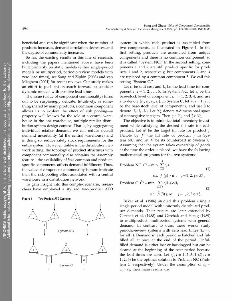
chers have employed a stylized two-product ATO

Figure 1 Two-Product ATO Systems

1

1

1

1 2

2

2

2

5

43

System NC

System C

system in which each product is assembled fromtwo components, as illustrated in Figure 1. In thefirst setting, products are assembled from uniquecomponents and there is no common component, soit is called “System NC.” In the second setting, com-ponents 1 and 2 are still product specific for prod-ucts 1 and 2, respectively, but components 3 and 4are replaced by a common component 5. We call thissetting “System C.”Let ci be unit cost and Li be the lead time for com-

ponent i, i = 1�2� � � � �5. In System NC, let si be thebase-stock level of component i, i= 1�2�3�4, and uses to denote �s1� s2� s3� s4�. In System C, let s̃i, i= 1�2�5be the base-stock level of component i, and use s̃ todenote �s̃1� s̃2� s̃5�. Let �n

+ denote n-dimensional spaceof nonnegative integers. Then s ∈�4+ and s̃ ∈�3+.The objective is to minimize total inventory invest-

ment while satisfying the desired fill rate for eachproduct. Let j be the target fill rate for product j .Denote by f j the fill rate of product j in Sys-tem NC, and let f̃ j be its counterpart in System C.Assuming that the system takes ownership of goodsat the time the order is placed, we have the followingmathematical programs for the two systems:

Problem NC C∗=min4∑i=1cisi

s.t. f j�s�≥j� j=1�2� s∈�4+�(1)

Problem C �C∗=min ∑i=1�2

cis̃i+c5s̃5

s.t. f̃ j � s̃�≥j� j=1�2� s̃∈�3+�(2)

Baker et al. (1986) studied this problem using asingle-period model with uniformly distributed prod-uct demands. Their results are later extended byGerchak et al. (1988) and Gerchak and Henig (1989)to multiproduct, multiperiod systems with generaldemand. In contrast to ours, these works studyperiodic-review systems with zero lead times (Li = 0for all i). Demand in each period is batched and ful-filled all at once at the end of the period. Unful-filled demand is either lost or backlogged but can becleared at the beginning of the next period becausethe lead times are zero. Let s∗i � i = 1�2�3�4 (s̃∗i � i =1�2�5) be the optimal solution to Problem NC (Prob-lem C, respectively). Under the assumption of c3 =c4 = c5, their main results are:

INFORMS

holds

copyrightto

this

article

and

distrib

uted

this

copy

asa

courtesy

tothe

author(s).

Add

ition

alinform

ation,

includ

ingrig

htsan

dpe

rmission

policies,

isav

ailableat

http://journa

ls.in

form

s.org/.

Song and Zhao: Value of Component CommonalityManufacturing & Service Operations Management 11(3), pp. 493–508, © 2009 INFORMS 495

Property (P1). �C∗ ≤ C∗. That is, the introductionof commonality reduces the total inventory investmentrequired to maintain a specific service level.

Property (P2). If c1 = c2, then s̃∗5 ≤ s∗3 + s∗4 . That is,when the product-specific components have identical costs,the optimal stock level of the common component is lowerthan the combined optimal stock levels it replaces.

Property (P3). If c1 = c2, then s̃∗i ≥ s∗i , i = 1�2. Thatis, when the product-specific components have identicalcosts, the combined optimal stock levels of product-specificcomponents are higher with commonality than without it.

A natural question arises at this point: will theseresults still hold in dynamic models with lead times?If component costs and lead times are the same beforeand after component sharing, then it can be shownthat the optimal policy of System NC is always fea-sible for System C (i.e., it satisfies the fill rate con-straints). This is true because such a policy is a specialcase of those of System C, which partition the inven-tory of a common component into separate bins, eachcommitted to a product. Therefore, the optimal inven-tory investment of System C should be no greaterthan that of System NC. The problem is, the optimalpolicy of System C is not known, so we do not knowhow to achieve its optimal cost.The control of an ATO system consists of two deci-

sions: inventory replenishment and inventory alloca-tion. If the objective is to minimize long-run inventoryholding and backorder penalty costs, then the optimaldecisions are generally state dependent (see Song andZipkin 2003). Recently, Benjaafar and ElHafsi (2006)consider a special case: an assembly system witha single end product and multiple demand classes.Each component supplier has a finite productioncapacity. The authors show that under Markovianassumptions, the optimal replenishment policy is astate-dependent base-stock policy, and the optimalallocation rule is a multilevel rationing policy thatdepends on the inventory levels of all other compo-nents. Obviously, the optimal policy for a general mul-tiproduct ATO system is even more complex.For these reasons, only simple but suboptimal re-

plenishment and allocation policies are implementedin practice. When a suboptimal policy is used, it isnot obvious whether component commonality can

always yield inventory savings. Indeed, Song (2002)examines a model with constant lead times follow-ing an independent base-stock policy and the first-in-first-out (FIFO) stock-allocation rule. In a numericalstudy, she shows that with the same level of inventoryinvestment, component sharing can result in moreproduct backorders. This observation motivated us toanalyze this issue more thoroughly.Consistent with practice, we focus on some sim-

ple but commonly used suboptimal policies. First,we assume that state-independent base-stock policies areemployed for inventory replenishment. In the contin-uous-review system we consider, this policy impliesthat a replenishment order is placed for each requiredcomponent at each demand arrival—the so-called one-for-one replenishment policy. Second, we consider twocomponent allocation rules—the FIFO rule and a mod-ified first-in-first-out (MFIFO) rule. We describe themin detail below.Under FIFO, demand for each component is ful-

filled in exactly the same sequence as it occurs. Thisis a component-based allocation rule, because the allo-cation of one component’s inventory does not dependon the inventory status of other components. Whena product demand arrives, if some of its componentsare available while others are not, the available com-ponents are put aside as committed stock. When acomponent is replenished, we commit it to the oldestbackordered product that requires it. This rule is sub-optimal because it commits available components tobacklogged demand, creating extra waiting time forboth the available components and for other demand.The virtue of this rule is simplicity of its informationrequirements and implementation. Moreover, it is per-ceived to be fair to the customers.Under MFIFO, product demand is filled following

the FIFO rule as long as all components demandedare available. When a product demand arrives andsome of its components are not available, however,we assign the demand to the last position in thebackorder list and do not allocate or commit thoseavailable components to the order. That is, a unitof component inventory will not be allocated to anincoming order unless such an allocation results in thecompletion of the order fulfillment. When a replenish-ment shipment arrives, we review the backorder listand satisfy the oldest backorder for which all required

INFORMS

holds

copyrightto

this

article

and

distrib

uted

this

copy

asa

courtesy

tothe

author(s).

Add

ition

alinform

ation,

includ

ingrig

htsan

dpe

rmission

policies,

isav

ailableat

http://journa

ls.in

form

s.org/.


components are available. This is a product-based allo-cation rule; the allocation of one component’s inven-tory to a demand depends on the inventory statusof other components. Consequently, it requires moreinformation and more coordination than FIFO. It alsomay make some orders wait longer than under FIFO.Note that we consider the total inventory invest-

ment (in the base-stock levels) as the objective func-tion in this paper. Although it is a common choicein the inventory literature, the objective function doesnot account for the extra holding costs charged in theFIFO system for the committed components. Includ-ing these costs would affect the economics of the FIFOallocation rule adversely.Both FIFO and MFIFO are common in practice.

Kapuscinski et al. (2004) describe an example ofMFIFO at Dell, and Cheng et al. (2002) describe anexample of FIFO at IBM.Section 3 focuses on the FIFO system and §4 ana-

lyzes the system under MFIFO. To the best of ourknowledge, our analysis provides the first closed-form evaluation of an allocation rule more complexthan FIFO. We also show that the closed-form evalu-ation works for a class of no-holdback allocation rulesthat do not holdback on-hand inventory when back-orders exist, which includes MFIFO as a special case.In addition, we show that, for any given base-stockpolicy, MFIFO achieves the same product fill rates asany other no-holdback rule. So the results on MFIFOapply to all no-holdback rules.Equipped with the analytical tools, we show that,

in the case of equal lead times across components,Properties (P1)–(P3) hold under MFIFO, but Proper-ties (P1) and (P2) do not hold under FIFO. In the caseof unequal lead times, Properties (P1)–(P3) fail to holdunder both FIFO and MFIFO. Thus, under these com-monly used allocation rules, component commonal-ity does not always provide inventory benefits. Ouranalysis further sheds light on why this could hap-pen. One important implication of these observationsis that product structure (i.e., making several prod-ucts share some common components) alone may notnecessarily lead to inventory savings. We also needan effective operational policy specially tailored to thenew product structure.To identify when component commonality is more

likely to yield inventory benefit under the simple con-trol policies considered here, and to quantify such

benefit, in §5 we perform an asymptotic analysison the system parameters. The analysis applies toboth FIFO and MFIFO. We also conduct an exten-sive numerical study in §6 to examine the value ofcommonality when the parameters are in between theasymptotic limits. In general, we find that compo-nent sharing is beneficial under these simple policies.The resulting inventory savings are more significantunder MFIFO or when the common component ismore expensive or has a longer lead time than theproduct-specific components. At an extreme, whenthe costs of the product-specific components are neg-ligible relative to that of the common component, thevalue of the component commonality converges tothe risk-pooling effect associated with a central ware-house in the distribution network setting. This is themaximum inventory benefit component commonalitycan achieve. We also find that the performance gapbetween MFIFO and FIFO tends to be higher as thetarget fill rate decreases or when the common compo-nent has a shorter lead time than the product-specificcomponents. Finally, in §7, we summarize the insightsand conclude the paper.

2. Other Related LiteratureIn the literature of dynamic ATO systems with positivelead times, most papers assume independent base-stock replenishment policies; see Song and Zipkin(2003) for a survey. For continuous-review models(which is the setting in this paper), to our knowledge,all papers consider the FIFO allocation rule; see, forexample, Song (1998, 2002), Song et al. (1999), Songand Yao (2002), and Lu et al. (2003, 2005), and Zhaoand Simchi-Levi (2006). For periodic-review models,because the demands during each period are batchedand filled at the end of the period, different allo-cation rules have been considered. These include afixed priority rule by Zhang (1997), the FIFO rule byHausman et al. (1998), a fair-share rule by Agrawaland Cohen (2001), and a product-based allocation ruleby Akcay and Xu (2004). However, all these studiesapply FIFO for demands between periods. In otherwords, if implemented in a continuous-review envi-ronment, these alternative allocation rules reduce toFIFO. The policy choices in the asymptotic studies byPlambeck and Ward (2006, 2007) on high-volume ATO

INFORMS

holds

copyrightto

this

article

and

distrib

uted

this

copy

asa

courtesy

tothe

author(s).

Add

ition

alinform

ation,

includ

ingrig

htsan

dpe

rmission

policies,

isav

ailableat

http://journa

ls.in

form

s.org/.


systems are exceptions, but their setting is quite dif-ferent from ours. There, the decision variables includethe component production capacities, product pro-duction sequence, and product prices. Once a compo-nent’s production capacity is chosen, the productionfacility produces the component at full capacity, sothere is no inventory decision.In addition to Song (2002), several other authors

conduct numerical experiments to study the value ofcomponent commonality in systems with lead times,using the analytical tools developed in their papers.For example, Agrawal and Cohen (2001) considerperiodic-review assembly systems with constant leadtimes. Component inventories are managed by base-stock policies and common components are allocatedaccording to the fair-share rule. Assuming that thedemands for components follow a multivariate nor-mal distribution, the authors study a four-product,two-component example numerically and show thata higher degree of commonality leads to lower costs.Cheng et al. (2002) study configure-to-order systemsbased on real-world applications from IBM. Commoncomponents are allocated according to the FIFO rule,and component replenishment lead times are stochas-tic. The authors develop an approximation for order-based service levels. Using numerical studies, theyshow that for given service levels, up to a 25�8%reduction of component inventory investments canbe achieved by sharing components, and the sav-ings increase as the number of associated productsincreases. Our analytical results are consistent withthe observations of these studies.It is worth mentioning that Alfaro and Corbett

(2003) also point out that the effect of pooling maybe negative when the inventory policy in use is sub-optimal. However, their study focuses on a singlecomponent only, analogous to the warehouse setting.Thus, they do not consider the assembly operation.Moreover, they use a single-period model, so compo-nent lead time is not an issue. Finally, in their setting,the form of the optimal policy is known, and theyuse suboptimal policy parameters to conduct theirstudy. In our setting, the form of the optimal policy isunknown, so we focus on a class of suboptimal poli-cies that is widely used in practice. But within thisclass of policies, our study assumes that the policyparameters are optimized.

Rudi (2000) studies the impact of component coston the value of commonality in a single-period model.He shows qualitatively that a more expensive commoncomponent leads to higher savings from commonality.Our work complements his study by examining adynamic system with positive lead times and quan-tifying the component cost effect through asymptoticresults and numerical examples.It is common in the literature to approximate the

value of component commonality by the risk-poolingeffect associated with a central warehouse (Eppen1979). See, for example, Chopra and Meindl (2001),Simchi-Levi et al. (2003), and Thonemann and Bran-deau (2000). This approximation, however, ignores theimpact of the product-specific components and there-fore may overestimate the benefits. In this paper, wedevelop insights on when this approximation is rea-sonably accurate and when it is not.Finally, we note that Thonemann and Bradley

(2002) conduct asymptotic analysis on the effect ofsetup times on the cost of product variety by lettingthe number of products approach infinity. Their focusand model setting, as well as the type of limit, are alldifferent from ours.

3. Analysis Under FIFOThis section focuses on the two-product ATO systemdescribed in §1 (see Figure 1) under the FIFO ruleand discusses the validity of Properties (P1)–(P3). Thissimple system connects well with the existing litera-ture on static models without lead times. It also laysthe foundation for the more general systems consid-ered in §5.We assume that demand for product j forms a

Poisson process (unit demand) with rate �j , j =1�2, and one unit of each component is needed toassemble one unit of final product. The inventoryof each component is controlled by an independentcontinuous-time base-stock policy with an integerbase-stock level. Replenishment lead times of compo-nents are constant but not necessarily identical.

3.1. Fill Rate ComparisonTo compare the solutions of Problem NC with Prob-lem C under the FIFO rule, it is important to under-stand the relationship between fill rates f j and f̃ j . BySong (1998), for j = 1�2,

INFORMS

holds

copyrightto

this

article

and

distrib

uted

this

copy

asa

courtesy

tothe

author(s).

Add

ition

alinform

ation,

includ

ingrig

htsan

dpe

rmission

policies,

isav

ailableat

http://journa

ls.in

form

s.org/.


f j = Pr{Dj�Lj� < sj�D2+j �L2+j � < s2+j} (3)

f̃ j = Pr{Dj�Lj� < s̃j�D5�L5� < s̃5}� (4)

where Di�Li�, i= 1�2� � � � �5, are the lead-time demandfor components. Let Dj�L� be the demand for prod-uct j during time L. Then,

Di�L�=D2+i�L�=Di�L�� i= 1�2� (5)

D5�L�=D1�L�+D2�L�� (6)

To examine Properties (P1)–(P3), we assume thatboth the common component 5 and the componentsthat it replaces have the same cost and lead time; i.e.,ci = c′ and Li = L′, i = 3�4�5. The following proposi-tion shows that the optimal solution in System NCmay not be feasible in System C under the FIFO rule.

Proposition 1. Assume the same lead time across allcomponents; i.e., L1 = L2 = L and L′ = L. If the base-stocklevels of the product-specific components are the same inSystem NC and System C, i.e., s̃i = s∗i , i= 1�2, then(a) the order-based fill rates in System NC are greater

than their counterparts in System C for any finite s̃5.That is,

f j > f̃ j� j = 1�2� (7)

(b) The solution s̃ = �s∗1� s∗2� s∗3 + s∗4� may not be feasiblefor System C.

Proof. By L′ = L and Equation (5), the optimalbase-stock levels in System NC must satisfy

s∗j = s∗2+j � j = 1�2� (8)

For any finite integer s̃5 and j = 1�2, by Equa-tions (3)–(6) and (8),

f j = Pr�Dj�L� < s∗j �Dj�L� < s∗2+j �= Pr�Dj�L� < s∗j �= Pr�Dj�L� < s̃j �> Pr�Dj�L� < s̃j�D

1�L�+D2�L� < s̃5�= f̃ j � (9)

proving (a). Note that the target fill rate j can chooseany real number in �0�1�, so Part (b) is a direct conse-quence of Part (a). �

Proposition 1(a) offers some interesting insights.Note that the first equality in (9) holds becauseDj�L� = D2+j �L� = Dj�L� in any event (Equation (5)).So, with equal component lead times, the supplies ofthe two components for product j in System NC are

completely synchronized. Replacing components 3and 4 by a common component 5 disrupts this syn-chronization: because D5�L� includes the demand forall products, it is only partially correlated with Dj�L�,j = 1�2. In other words, the supply process of thecommon component is only partially correlated withthe supply process of the product-specific compo-nent. Because of the assembly feature, it is then intu-itive that the less-synchronized component supplyprocesses in System C result in smaller order-basedfill rates. (Indeed, inequality (9) provides an analyti-cal explanation for the numerical observation of Song2002 mentioned in §1.)In a single-period model or periodic review systems

with zero lead times, if one keeps the stock levelsof the product-specific components unchanged andlets the stock level of the common component be thesum of stock levels of those it replaces, the optimalsolution without component sharing is always feasi-ble for the corresponding component sharing system(see, e.g., Baker et al. 1986). Proposition 1(b) indicatesthat this statement does not hold in dynamic systemswith lead times under the FIFO rule.

3.2. Counterexamples to Properties (P1)–(P3)In this section, we show that although Property (P3)holds for the equal lead-time case, it fails to hold forthe unequal lead-time case. We also show that Prop-erties (P1) and (P2) do not hold even for the equallead-time case.Observation 1. Assume the same lead time across

all components. Then Property (P3) holds under FIFO.That is, the optimal product-specific base-stock levelsin System C are no less than those in System NC.Proof. See the online appendix for details. �

Observation 2. Assume the same lead time acrossall components. Then Properties (P1) and (P2) do nothold. That is, for the same target service levels, Sys-tem C may require higher optimal inventory invest-ment than System NC, so component commonalitydoes not always lead to inventory benefit. Also, theoptimal stock level of the common component mayexceed the combined stock levels it replaces.Proof. It suffices to construct numerical counterex-

amples to Properties (P1) and (P2). Considering asymmetric two-product system with L= L′, c1 = c2 =c, c′ = 1, j = , �j = 1, j = 1�2. Because of symmetry,

INFORMS

holds

copyrightto

this

article

and

distrib

uted

this

copy

asa

courtesy

tothe

author(s).

Add

ition

alinform

ation,

includ

ingrig

htsan

dpe

rmission

policies,

isav

ailableat

http://journa

ls.in

form

s.org/.


Table 1 Counterexamples to Properties (P1) and (P2) Under FIFO

Solution (NC) Solution (C) Fill rate (C)� (%) L c/c′ Savings (%) �s∗1� s

∗3� Fill rate (NC) (%) �s̃∗1� s̃

∗5� Fill rate (C) (%) s̃1 = s∗1, s̃5 = s∗3 + s∗4 (%)

95 10 5 −104 �16�16� 9513 �16�34� 9506 948495 10 10 −057 �16�16� 9513 �16�34� 9506 948495 10 50 −012 �16�16� 9513 �16�34� 9506 948470 1 1 −125 �2�2� 735 �2�5� 727 6992

we only need to consider product 1 and its associ-ated components, 1, 3, and 5. Numerical results aresummarized in Table 1, where the percentage savingsrefers to the relative reduction of the total inventoryinvestment from Problem NC to Problem C, i.e., 100 ∗�C∗ − �C∗�/C∗. We use enumeration based on Equa-tions (3)–(4) to obtain the optimal solutions for Prob-lem NC and Problem C.In these numerical examples, C∗ < �C∗ and s̃∗5 > 2s

∗3 .

The first fact implies that Property (P1) may not hold;the second fact indicates that Property (P2) may nothold because s∗3 + s∗4 = 2s∗3 , because of symmetry. �

We now provide insight into the counterexamples.In the first three cases of Table 1, c/c′ is high (c/c′ =5�10�50); i.e., the common component is inexpen-sive relative to product-specific components. If weset �s̃1� s̃5� = �16�32�, the fill rate of System C is94�8% �<95%� (which is possible by Proposition 1). Toachieve the target fill rate of 95% in System C, we onlyhave two options: (i) increasing s̃i from 16 for at leastone product-specific component i = 1�2, or (ii) keep-ing s̃i = 16, i= 1�2 but increasing s̃5 from 32 until thefill rate constraint(s) are satisfied. For convenience, wecall option (i) the specific option and option (ii) thecommon option.Clearly, the specific option increases the inven-

tory investment of the product-specific component(s),and the common option only increases the inventoryinvestment of the common component. Because c′ � c

in these cases, it turns out that the optimal solutionhere is to increase the base-stock level of the commoncomponent to 34 while keeping the base-stock levels

Table 2 A Counterexample to Property (P3) Under FIFO

Solution (NC) Solution (C)c/c′ �s∗1� s

∗3� Fill rate (NC) �s̃∗1� s̃

∗5� Fill rate (C)

0.1 �8�16� 95.08% �6�29� 95.19%

of product-specific components unchanged. It is inter-esting to note that in these cases, the optimal solutionsin Problem NC not only have lower total inventoryinvestments but also have higher fill rates (95�13%),than their counterparts in Problem C (95�06%).The last case of Table 1 shows that counterexam-

ples can occur even when the common componentis not so inexpensive relative to the product-specificcomponents.Observation 3. Property (P3) may not hold if L1 =

L2 = L but L = L′. That is, when the common com-ponent has a different lead time from those of theproduct-specific components, the combined optimalstock levels of product-specific components may belower in System C than in System NC; i.e., s̃∗1 can besmaller than s∗1 . See Table 2 for an example, whereL1 = L2 = L = 2, L′ = 10, c1 = c2 = c = 0�1, c′ = 1,j = 95%, �j = 1, j = 1�2.Intuitively, when L = L′, s∗1 may not be the small-

est integer, such that Pr�D1�L� < s∗1� ≥ 0�95. This isespecially true when c� c′, because in this case, theoptimal solution in Problem NC is to keep s∗3 at theminimum while increasing s1 until the solution is fea-sible. While in Problem NC, the cost of increasing s1(or s3) by one unit is 2∗c (2∗c′, respectively); in Prob-lem C, the cost of increasing s̃1 (or s̃5) by one unit is2 ∗ c (c′, respectively). Therefore, the relative cost ofincreasing the stock levels of product-specific compo-nents is higher in Problem C than in Problem NC,which implies that s̃∗1 can be smaller than s

∗1 . Inter-

estingly, we also have s̃∗5 < s∗3 + s∗4 in this example

because c� c′.

4. Analysis Under MFIFOIn this section, we consider the same product struc-tures as in §3 (see Figure 1), but under the MFIFOrule. All other assumptions and notations remain thesame.

INFORMS

holds

copyrightto

this

article

and

distrib

uted

this

copy

asa

courtesy

tothe

author(s).

Add

ition

alinform

ation,

includ

ingrig

htsan

dpe

rmission

policies,

isav

ailableat

http://journa

ls.in

form

s.org/.


We first note that MFIFO belongs to a general classof reasonable allocation rules for System C that do nothold back stock when backorders exist. In particular,they satisfy the following condition:

Bi�t� ∗min�Ii�t�� I5�t��= 0� i= 1�2� for all t ≥ 0�(10)

where Ii�t� and Bj�t� are the on-hand inventory ofcomponent i and backorders of product j at time t,respectively. Thus, under any rule that satisfies thisproperty, a demand is backordered if and only ifat least one of its components runs out of on-handinventory. For this reason, we call rules that satisfyCondition (10) no-holdback rules.MFIFO is a no-holdback rule. Other no-holdback

rules may allocate available inventory to backordereddemand in different sequences from FIFO. For any no-holdback rule, we assume that demand for the sameproduct is satisfied on a FIFO basis. In the next sub-section, we show that, for any given base-stock pol-icy, MFIFO achieves the same fill rates as any otherno-holdback rule. Thus, under the framework of min-imizing the total inventory investments subject to fillrate constraints, comparing MFIFO with FIFO is thesame as comparing any no-holdback rule with FIFO.

4.1. Fill Rate ExpressionsProposition 2. Under any given base-stock policy in

System C1. The fill-rates under MFIFO can be expressed as

follows�

f̃ 1 = Pr{D1�L1� < s̃1�D1�L′�+D2�L′�− �D2�L2�− s̃2�+ < s̃5

}� (11)

f̃ 2 = Pr{D2�L2� < s̃2�D1�L′�+D2�L′�− �D1�L1�− s̃1�+ < s̃5

}� (12)

Note that B2 = �D2�L2� − s̃2�+ (or B1 = �D1�L1� − s̃1�+)is the number of backorders of product-specific compo-nent 2 (or 1).2. MFIFO always outperforms FIFO on the fill rates.3. MFIFO has identical fill rates as any other no-hold-

back rule.

Proof. See the online appendix for details. �

In the rest of this section, we shall focus on MFIFO.By Proposition 2, we note that all results of MFIFOapply equally to no-holdback rules.

4.2. Properties (P1)–(P3): Equal Lead TimesIn this subsection we assume the same system set-tings studied in §3.1. We show that here, unlike thecase under FIFO, Properties (P1)–(P3) hold true underMFIFO. Hence, commonality cannot hurt.First, we show that, under MFIFO, the optimal solu-

tion for System NC achieves the same product fillrates in System C, which implies Property (P1). Thatis:

Proposition 3. Suppose Li = L′ for all i and ci = c′,i= 3�4�5. In addition, L1 = L2 = L and L′ = L. Let s̃i = s∗i ,i= 1�2, and s̃5 = s∗3 + s∗4 . Then, under MFIFO,

f̃ j = f j� j = 1�2� (13)

Hence, the solution s̃ = �s∗1� s∗2� s∗3 + s∗4� is feasible in Sys-tem C. Therefore, Property (P1) holds.

Proof. See the online appendix for details. �

For Properties (P2) and (P3), we have

Proposition 4. Under MFIFO and equal lead times,

s̃∗5 ≤ s∗3 + s∗4� (14)

s̃∗i ≥ s∗i � i= 1�2� (15)

So, Properties (P2) and (P3) hold even for nonidentical ci,i= 1�2.Proof. See the online appendix for details. �

4.3. Properties (P1)–(P3): Unequal Lead TimesThe main result in this subsection is the followingobservation:Observation 4. When the lead times are not iden-

tical, Properties (P1)–(P3) may not hold under MFIFO.When �j , Li, and ci are different for j = 1�2, i= 1�2,

we have found counterexamples to Properties (P1)and (P2). Table 3 presents one of them, with �1 = 1,�2 = 2.In this example, using the optimal System NC solu-

tion in System C, i.e., assuming �s̃1� s̃2� s̃5�= �11�8�46�,we have �f̃ 1� f̃ 2�= �89�99%�94�69%�, missing the tar-get fill rate for product 1. Because the base-stock lev-els can only choose integers, making up the smalldeterioration can lead to sizable increase in inventoryinvestment, which results in higher inventory invest-ment in System C than in System NC.

INFORMS

holds

copyrightto

this

article

and

distrib

uted

this

copy

asa

courtesy

tothe

author(s).

Add

ition

alinform

ation,

includ

ingrig

htsan

dpe

rmission

policies,

isav

ailableat

http://journa

ls.in

form

s.org/.


Table 3 A Counterexample to Properties (P1) and (P2) Under MFIFO

Solution (NC) Fill rates (NC) Solution (C) Fill rates (C)� �c1� c2� c

′� �L1� L2� L′� Savings (%) �s∗1� s

∗3�, �s

∗2� s

∗4� �f 1� f 2� �s̃∗1� s̃

∗2� s̃

∗5� �f̃ 1� f̃ 2�

90% �10�10�1� �7�2�10� −042% �11�18�, �8�28� �9000%�9085%� �11�8�47� �9006%�9477%�

It turns out that the counterexample in §3.2 forProperty (P3) under FIFO (see Table 2) is also acounterexample for Property (P3) under MFIFO; seeTable 4. Here, the solution for System C stays thesame under both FIFO and MFIFO. The example alsoconfirms the result in §4.2; i.e., with the same base-stock levels, MFIFO yields higher fill rates than FIFO(see Tables 2 and 4).So far, we have provided some insight on when

commonality always generates inventory benefitsand constructed counterexamples on when it doesnot. The counterexamples, although occurring infre-quently and yielding minor losses, caution the use ofthis strategy in dynamic ATO systems. To provide amore comprehensive picture on the impact of compo-nent commonality, we conducted an asymptotic anal-ysis and a numerical study to quantify the value ofcommonality and its sensitivity.

5. Asymptotic AnalysisThe counterexamples in the previous section indicatethat if the common component is inexpensive rela-tive to product-specific components, the value of com-monality may be low. Thus, it is natural to ask: doesit always pay to share expensive components in sys-tems with lead times? More importantly, what is theimpact of component cost, lead time, and target fillrate on component commonality? We address thesequestions in this section.To gain more insight, we consider a more general

product structure than the one considered in the pre-vious section. In particular, instead of two products,we now assume that there are N products. Again, eachproduct is made of two components, and we still usei to index components and j to index products. In the

Table 4 Counterexample to Property (P3) Under MFIFO

Soln. (NC) Soln. (C)c/c′ �s∗1� s

∗3� Fill rate (NC) �s̃∗1� s̃

∗5� Fill rate (C)

0.1 �8�16� 95.08% �6�29� 95.22%

original system without component sharing, i.e, Sys-tem NC, product j is assembled from two unique com-ponents j and N + j . In a revised system, System C, wereplace components N + 1, N + 2� � � � �2N with com-mon component 2N + 1, so product j is assembledfrom the product-specific component j and the com-mon component 2N + 1.All other features and notations of the model stay

the same as in the two-product system in §§1 and 3.As before, we assume that all components replacedby the common component have an identical unit costof c′ and an identical lead time of L′, and that aftercomponent sharing, unit cost and lead time do notchange. In other words, ci = c′ and Li = L′, i=N + 1�N + 2� � � � �2N + 1.The mathematical programs for System-NC and

System C (the counterparts of (1) and (2)) are givenas follows:

Problem NC C∗ =min2N∑i=1cisi

s.t. f j�s�≥ j�j = 1�2� � � � �N� �si� ∈�2N+ �

(16)

Problem C �C∗ =minN∑i=1cis̃i+ c′ s̃2N+1

s.t. f̃ j � s̃�≥ j�j = 1�2� � � � �N� �s̃i� ∈�N+1

+ �

(17)

where

f j�s�= Pr�Dj�Lj� < sj�Dj�L′� < sN+j �� (18)

f̃ j � s̃�= Pr{Dj�Lj� < s̃j�

N∑l=1Dl�L′� < s̃2N+1

}�

under FIFO� (19)

f̃ j � s̃�= Pr{Dj�Lj�<s̃j�

N∑l=1Dl�L′�− ∑

l=1��N�l =jBl < s̃2N+1

}�

under MFIFO� (20)

INFORMS

holds

copyrightto

this

article

and

distrib

uted

this

copy

asa

courtesy

tothe

author(s).

Add

ition

alinform

ation,

includ

ingrig

htsan

dpe

rmission

policies,

isav

ailableat

http://journa

ls.in

form

s.org/.


Here, Bl is the number of backorders of component lin steady state. Equations (18)–(19) are straightfor-ward extensions of Equations (3)–(4). Equation (20) isan extension of Equation (11) of N = 2; see the onlineappendix for a detailed discussion.

5.1. Effect of Sharing Expensive ComponentsLet us first consider the effect of sharing expensivecomponents, such as using common central process-ing units in Personal Computers and common air-conditioning systems in automobiles. We do so byassuming ci/c′ → 0, i= 1�2� � � � �N . Under this condi-tion, Problem NC (16) and Problem C (17) reduce to

Problem NC(0) min c′2N∑

i=N+1si

s.t. Pr�Dj�L′� < sN+j �≥ j�j = 1�2� � � � �N �

(21)

Problem C(0) min c′ s̃2N+1

s.t. Pr{ N∑l=1Dl�L′� < s̃2N+1

}≥ j�

j = 1�2� � � � �N �

(22)

This holds true because in the limit, we can increasebase-stock levels of the product-specific componentswithout increasing total inventory investments. Thisimplies that for all product-specific components, wecan always ensure Di�Li� < si (and hence Bi = 0),i= 1� � � � �N without increasing objective function val-ues. Therefore, the fill rates are determined only bycomponents i = N + 1� � � � �2N in System NC and bycommon component i= 2N +1 in System C. Note thatProblem C(0) has identical form under either FIFO orMFIFO.To study the impact of component commonality,

we follow standard procedure by assuming j = for all j and approximating the Poisson lead timedemand DN+j �t − L′� t� by a normal random variablewith mean L′�j and standard deviation

√L′�j . (This

approximation is reasonably accurate when L′�j is nottoo small, e.g., L′�j ≥ 10.) Let ��·� be the standard nor-mal distribution, and denote z =�−1��. Consistentwith practice, we assume > 50% and so z > 0. Thenfor System NC,

s∗N+j = L′�j + z√L′�j � (23)

Thus, the optimal objective value of Problem NC(0)equals c′L′

∑Nj=1 �

j + c′z√L′∑Nj=1

√�j . Following the

same logic, for Problem C(0) we have,

s̃∗2N+1 = L′N∑j=1�j + z

√L′

√√√√ N∑j=1�j � (24)

Hence, the optimal objective value of Problem C(0) isc′ s̃∗2N+1. Note that both Equations (23) and (24) includetwo terms; the first term represents the pipelineinventory and the second term represents the safetystock. The effect of lead time is predominately onpipeline inventory (O�L′�) rather than on safety stock(O�

√L′�).

By Equations (23) and (24),

Value of Component Commonality

≡Relative Reduction on Inventory Investmentfrom System NC to System C (25)

=∑Nj=1

√�j −

√∑Nj=1 �j√

L′∑Nj=1 �j/z+

∑Nj=1

√�jin case of ci/c

′ → 0�

i= 1�2� � � � �N � (26)

When expressed in terms of percentage, we also referto (25) as the percentage savings of component shar-ing. Equation (26) shows that, in the special caseof ci � c′, the value of component commonality isalways greater than or equal to zero. Note that includ-ing the pipeline inventory in Equation (26) reducesthe value of commonality and makes it sensitive tothe changes in lead times and fill rates.To see clearly the impact of the system parameters,

we consider the symmetric case of �j = �, for all j .Under this setting, (26) is simplified to

(z

z+√�L′

)(1− 1√

N

)� (27)

Thus, when ci � c′, the value of component com-monality increases as (i) the target service level increases, (ii) the lead time for the common compo-nent L′ decreases, and (iii) the number of productsthat share the common component N increases at arate proportional to the square root of N .In addition, in the case of symmetric products,

the total stock level of the common component in

INFORMS

holds

copyrightto

this

article

and

distrib

uted

this

copy

asa

courtesy

tothe

author(s).

Add

ition

alinform

ation,

includ

ingrig

htsan

dpe

rmission

policies,

isav

ailableat

http://journa

ls.in

form

s.org/.


System C (under either FIFO or MFIFO) is NL′� +z√NL′�. This resembles the “risk-pooling” effect

studied by Eppen (1979) for centralized stock. Indeed,Problem NC(0) can be viewed as a completely decen-tralized multilocation system, with separate inven-tory kept at each location to satisfy local demand;Problem C(0) can be viewed as a completely cen-tralized system with one central warehouse fulfillingall demands. (The “risk-pooling” effect refers to theobservation that expected inventory-related costs ina decentralized system exceed those in a centralizedsystem, and when demands are identical and uncor-related, the part of cost proportional to z

√NL′� in a

centralized system increases as the square root of thenumber of consolidated demands.)

5.2. Effect of Sharing Inexpensive ComponentsLet us next consider the effect of sharing inexpensivecomponents, such as using a common mouse in PCsand common spark plugs in automobiles. We do soby assuming c′/ci → 0 for i = 1�2� � � � �N . Under thiscondition, Problem NC (16) reduces to

Problem NC(�) minN∑i=1cisi

s.t. Pr�Dj�Lj� < sj�≥ j�j = 1�2� � � � �N �

(28)

Problem C (17) (under either FIFO or MFIFO)reduces to

Problem C(�) minN∑i=1cis̃i

s.t. Pr�Dj�Lj� < s̃j �≥ j�j = 1�2� � � � �N �

(29)

Observe that the mathematical programs (28) and (29)are identical; hence the value of component common-ality converges to zero as c′/ci → 0, i= 1�2� � � � �N .To summarize, we have shown the following

results.

Proposition 5. In the multiproduct System NC andSystem C, the following results hold under either FIFO orMFIFO:(a) Given c′, the value of component commonality con-

verges to that of the “risk-pooling” effect as ci/c′ → 0 forall i= 1�2� � � � �N .

(b) Given ci, i = 1�2� � � � �N , the value of compo-nent commonality converges to zero as c′/ci → 0 for alli= 1�2� � � � �N .Proposition 5 implies that, under general condi-

tions, if the common component is very expensive rel-ative to product-specific components, then the impactof component commonality is substantial. In fact, thevalue of component commonality converges to thatof the “risk-pooling” effect. On the other hand, if thecommon component is very cheap relative to all theproduct-specific components, component commonal-ity has little impact on inventory investments or ser-vice levels.

6. Numerical StudiesThe previous section quantifies the value of common-ality in the limiting cases of component costs. In thissection, we conduct a numerical study to quantify thevalue of component commonality between the twoasymptotic limits. We are interested in the impact ofcomponent costs and lead times and target fill rates.We also quantify the performance gap between FIFOand MFIFO rules. We shall connect results in this sec-tion to those in previous sections whenever possible.To develop managerial insights, we focus on the

simple two-product system (Figure 1) under the sym-metric assumption: �j = � and j = for j = 1�2;Li = L and ci = c for i= 1�2. Note that c = c′ and L = L′in general. Clearly, we must have identical s∗i and s̃

∗i

across i= 1�2 and identical s∗i for i= 3�4 under eitherFIFO or MFIFO.The mathematical programs (16) and (17) are solved

by enumeration based on the exact evaluation of thefill rates (see Equations (18)–(20)).

6.1. Parameter SetupThe system under study has the following parameters:�, c/c′, L′, L/L′, and . We choose the following valuesfor each parameter. � ∈ �1�2�5�; c/c′ ∈ �0�01�0�1�0�5�1�5�10�20�30�; L′ ∈ �1�2�5�10�20�; L/L′ ∈ �0�1�0�2�0�5�1�2�3�; and ∈ �0�7�0�75�0�8�0�85�0�9�0�95�. Given acombination of the parameters, we compute the valueof commonality under either FIFO or MFIFO.Because the base-stock levels can only choose inte-

gers, the target fill rate can rarely be achieved exactly.In fact, the difference between the target fill rate and

INFORMS

holds

copyrightto

this

article

and

distrib

uted

this

copy

asa

courtesy

tothe

author(s).

Add

ition

alinform

ation,

includ

ingrig

htsan

dpe

rmission

policies,

isav

ailableat

http://journa

ls.in

form

s.org/.


the actual fill rate can be high, e.g., up to 9% at� ∗L′ = 1. As � ∗ L′ increases, the integer base-stocklevel effect diminishes.

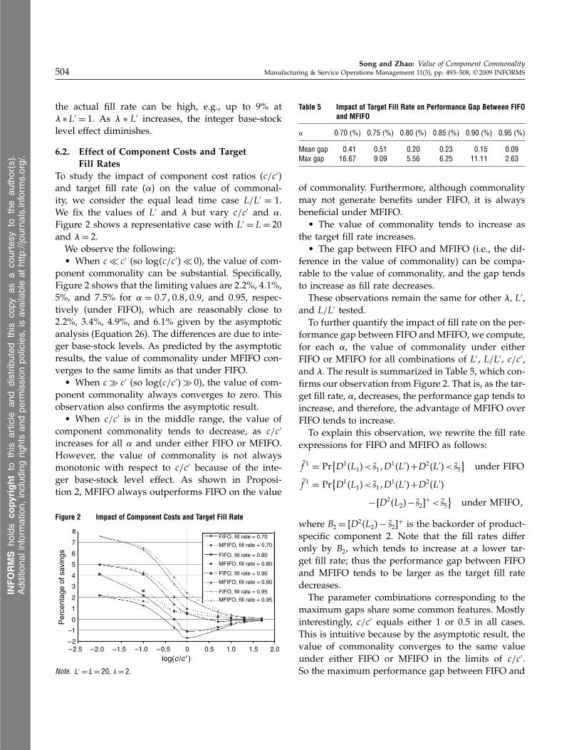
6.2. Effect of Component Costs and TargetFill Rates

To study the impact of component cost ratios (c/c′)and target fill rate () on the value of commonal-ity, we consider the equal lead time case L/L′ = 1.We fix the values of L′ and � but vary c/c′ and .Figure 2 shows a representative case with L′ = L= 20and �= 2.We observe the following:• When c� c′ (so log�c/c′�� 0), the value of com-

ponent commonality can be substantial. Specifically,Figure 2 shows that the limiting values are 2�2%, 4�1%,5%, and 7�5% for = 0�7�0�8�0�9, and 0�95, respec-tively (under FIFO), which are reasonably close to2�2%, 3�4%, 4�9%, and 6�1% given by the asymptoticanalysis (Equation 26). The differences are due to inte-ger base-stock levels. As predicted by the asymptoticresults, the value of commonality under MFIFO con-verges to the same limits as that under FIFO.• When c� c′ (so log�c/c′�� 0), the value of com-

ponent commonality always converges to zero. Thisobservation also confirms the asymptotic result.• When c/c′ is in the middle range, the value of

component commonality tends to decrease, as c/c′

increases for all and under either FIFO or MFIFO.However, the value of commonality is not alwaysmonotonic with respect to c/c′ because of the inte-ger base-stock level effect. As shown in Proposi-tion 2, MFIFO always outperforms FIFO on the value

Figure 2 Impact of Component Costs and Target Fill Rate

Per

cent

age

ofsa

ving

s

log(c /c ′ )

8

7

6

5

4

3

2

1

–1

0

–2–2.5 –0.5–1.5 0.5 1.51.0 2.00–2.0 –1.0

FIFO, fill rate = 0.70

MFIFO, fill rate = 0.70







Note. L′ = L= 20, �= 2.

Table 5 Impact of Target Fill Rate on Performance Gap Between FIFOand MFIFO

� 0.70 (%) 0.75 (%) 0.80 (%) 0.85 (%) 0.90 (%) 0.95 (%)

Mean gap 041 0.51 0.20 0.23 015 0.09Max gap 1667 9.09 5.56 6.25 1111 2.63

of commonality. Furthermore, although commonalitymay not generate benefits under FIFO, it is alwaysbeneficial under MFIFO.• The value of commonality tends to increase as

the target fill rate increases.• The gap between FIFO and MFIFO (i.e., the dif-

ference in the value of commonality) can be compa-rable to the value of commonality, and the gap tendsto increase as fill rate decreases.These observations remain the same for other �, L′,

and L/L′ tested.To further quantify the impact of fill rate on the per-

formance gap between FIFO and MFIFO, we compute,for each , the value of commonality under eitherFIFO or MFIFO for all combinations of L′, L/L′, c/c′,and �. The result is summarized in Table 5, which con-firms our observation from Figure 2. That is, as the tar-get fill rate, , decreases, the performance gap tends toincrease, and therefore, the advantage of MFIFO overFIFO tends to increase.To explain this observation, we rewrite the fill rate

expressions for FIFO and MFIFO as follows:

f̃ 1 = Pr{D1�L1�<s̃1�D1�L′�+D2�L′�<s̃5} under FIFO

f̃ 1 = Pr{D1�L1�<s̃1�D1�L′�+D2�L′�−�D2�L2�− s̃2�+<s̃5

}under MFIFO�

where B2 = �D2�L2�− s̃2�+ is the backorder of product-specific component 2. Note that the fill rates differonly by B2, which tends to increase at a lower tar-get fill rate; thus the performance gap between FIFOand MFIFO tends to be larger as the target fill ratedecreases.The parameter combinations corresponding to the

maximum gaps share some common features. Mostlyinterestingly, c/c′ equals either 1 or 0�5 in all cases.This is intuitive because by the asymptotic result, thevalue of commonality converges to the same valueunder either FIFO or MFIFO in the limits of c/c′.So the maximum performance gap between FIFO and

INFORMS

holds

copyrightto

this

article

and

distrib

uted

this

copy

asa

courtesy

tothe

author(s).

Add

ition

alinform

ation,

includ

ingrig

htsan

dpe

rmission

policies,

isav

ailableat

http://journa

ls.in

form

s.org/.


MFIFO is most likely to occur when c/c′ is equally faraway from the limits.

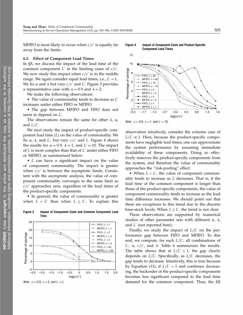
6.3. Effect of Component Lead TimesIn §5, we discuss the impact of the lead time of thecommon component L′ in the limiting cases of c/c′.We now study this impact when c/c′ is in the middlerange. We again consider equal lead times, i.e., L′ = L.We fix and � but vary c/c′ and L′. Figure 3 providesa representative case with = 0�9 and �= 2.We make the following observations:• The value of commonality tends to decrease as L′

increases under either FIFO or MFIFO.• The gap between MFIFO and FIFO does not

seem to depend on L′.The observations remain the same for other �, ,

and L/L′.We next study the impact of product-specific com-

ponent lead time (L) on the value of commonality. Wefix , �, and L′, but vary c/c′ and L. Figure 4 showsthe results for = 0�9, �= 1, and L′ = 10. The impactof L is more complex than that of L′ under either FIFOor MFIFO, as summarized below:• L can have a significant impact on the value

of component commonality. The impact is greaterwhen c/c′ is between the asymptotic limits. Consis-tent with the asymptotic analysis, the value of com-ponent commonality converges to the same limit asc/c′ approaches zero, regardless of the lead times ofthe product-specific components.• In general, the value of commonality is greater

when L < L′ than when L ≥ L′. To explain this

Figure 3 Impact of Component Costs and Common Component LeadTime

Per

cent

age

of s

avin

gs

log(c /c ′ )

25

20

15

10

5

–5

0

–2.5 –0.5–1.5 0.5 1.51.0 2.00–2.0 –1.0

FIFO, L′ = 1

MFIFO, L′ = 1

FIFO, L′ = 2

MFIFO, L′ = 2

FIFO, L′ = 5

MFIFO, L′ = 5

FIFO, L′ = 20MFIFO, L′ = 20

Note. �= 09, �= 2, and L′ = L.

Figure 4 Impact of Component Costs and Product-SpecificComponent Lead Times

Per

cent

age

of s

avin

gs

log(c /c ′)

12

10

8

6

4

2

0–2.2 –0.7 –0.2–1.7 0.3 0.8 1.3 1.8–1.2

FIFO, L = 30MFIFO, L = 30





Note. �= 09, �= 1, and L′ = 10.

observation intuitively, consider the extreme case ofL/L′ � 1. Here, because the product-specific compo-nents have negligible lead times, one can approximatethe system performance by assuming immediateavailability of these components. Doing so effec-tively removes the product-specific components fromthe system, and therefore the value of commonalityapproaches the “risk-pooling” effect.• When L < L′, the value of component common-

ality tends to increase as L decreases. That is, if thelead time of the common component is longer thanthose of the product-specific components, the value ofcomponent commonality tends to increase as the leadtime difference increases. We should point out thatthere are exceptions to this trend due to the discretebase-stock levels. When L≥ L′, the trend is not clear.These observations are supported by numerical

studies of other parameter sets with different , �,and L′ (not reported here).Finally, we study the impact of L/L′ on the per-

formance gap between FIFO and MFIFO. To thisend, we compute, for each L/L′, all combinations ofL′, , c/c′, and �. Table 6 summarizes the results.The table shows that at L/L′ ≤ 1, the gap clearlydepends on L/L′. Specifically, as L/L′ decreases, thegap tends to decrease. Intuitively, this is true becauseby Equation (11), if L/L′ < 1 and continues decreas-ing, the backorder of the product-specific componentsbecomes less significant compared to the lead timedemand for the common component. Thus, the fill

INFORMS

holds

copyrightto

this

article

and

distrib

uted

this

copy

asa

courtesy

tothe

author(s).

Add

ition

alinform

ation,

includ

ingrig

htsan

dpe

rmission

policies,

isav

ailableat

http://journa

ls.in

form

s.org/.


Table 6 Impact of L/L′ on Performance Gap Between FIFO and MFIFO

L/L′ 3 (%) 2 (%) 1 (%) 0.5 (%) 0.2 (%) 0.1 (%)

Mean gap 0.27 0.26 058 0.31 0.15 0.01Max gap 9.09 6.67 1667 7.14 5.56 1.35

rate difference between FIFO and MFIFO becomessmaller. However, at L/L′ > 1, the trend is not clear.The parameter combinations corresponding to the

maximum gaps here also share some commonfeatures. In addition to the fact that c/c′ equalseither 1 or 0�5 in all cases, the target fill rates are nomore than 80%, which confirms the result of Table 5.

7. Concluding RemarksWe have studied the value of component commonaltyand its sensitivity to system parameters in a class ofdynamic ATO systems with lead times. Because theoptimal policy is not known, we have assumed thatcomponent inventories are replenished by indepen-dent base-stock policies and are allocated accordingto either the FIFO or the MFIFO rule. These policiesare widely used in practice.Our analysis shows that although component com-

monality is generally beneficial, its value dependsstrongly on the component costs, lead times, andallocation rules (FIFO or MFIFO). In particular, com-monality does not guarantee inventory benefits forcertain systems, e.g., those with identical lead timesunder FIFO and those with nonidentical lead timesunder either FIFO or MFIFO. Yet with identical leadtimes and MFIFO, component commonality alwaysyields inventory benefits. We also show that MFIFOalways outperforms FIFO on the value of commonal-ity, and MFIFO achieves the same product fill rates asany other no-holdback rule. Using asymptotic analy-sis and a numerical study, we quantify the impact ofcomponent costs and lead times and target fill rateson the value of commonality and the performancegap between MFIFO and FIFO.It is worth mentioning that our objective function—

the total investment in the base-stock levels—is anapproximation of the component inventory-holdingcosts. This choice is common in the inventory litera-ture. It also facilitates the comparison with the staticmodel. However, this approximation does not accountfor the extra holding costs that are charged in the

FIFO system on the components that are reservedwhen the matching components are unavailable. Thisfact affects the economics of the FIFO allocation ruleadversely and thus further supports our results on thecomparison between FIFO and MFIFO.Our findings, such as those of Proposition 5, are

consistent with many industry practices, but not all.For example, in the medical equipment industry,a product family is often developed around a majorcomponent with long lead time (de Kok 2003). In theelectronics industry, different cell phone models canshare a platform (Whyte 2003), which is defined tobe a set of key (and therefore more expensive) com-ponents and subsystem assets (Krishnan and Gupta2001). In many other industries, however, both low-and high-value components are shared among dif-ferent product models. For computers, for example,the low-value common components include the key-board and mouse, and high-value common compo-nents include CPUs and hard drives. For automobiles,a low-value common component example is a sparkplug, and a high-value common component exampleis an air-conditioning system. This phenomenon mayreflect the fact that standardized components simplifyprocurement and exploit economies of scale in pro-duction, quality control, and logistics. Those featuresare not included in our model.For ease of exposition and tractability, we have

focused on the continuous-time base-stock policy forinventory replenishment. We note that, in practice,the batch-ordering policy is very common. Under thebatch-ordering policy, it is not clear whether Proposi-tions 1 and 3 still hold. But clearly, Proposition 5 canbe extended to handle batch orders. We also believethat counterexamples can be constructed under eitherFIFO or MFIFO because the fill rates of a batch order-ing system can be expressed as the averages of theircounterparts in the base-stock systems (Song 2000).A dynamic model with lead time differs from a

static model without lead time because in the former,both demand and replenishment arrive at the systemgradually, but in the latter, all demand and inventoryare present at the same time. Thus, in the dynamicmodel, lead times and the allocation rule that dynam-ically assigns common components to demand real-ized to date play important roles in realizing the valueof component commonality. As the present work

INFORMS

holds

copyrightto

this

article

and

distrib

uted

this

copy

asa

courtesy

tothe

author(s).

Add

ition

alinform

ation,

includ

ingrig

htsan

dpe

rmission

policies,

isav

ailableat

http://journa

ls.in

form

s.org/.


neared completion, we learned of the recently com-pleted work by Dogru et al. (2007). They establisheda lower bound for System C with equal constant leadtimes under the backorder-cost model (as opposed tothe service-level constrained model considered in ourpaper). They showed that MFIFO is the optimal allo-cation rule under certain symmetric conditions. How-ever, when the symmetric condition is violated or leadtimes are not identical, or when a service-level con-strained model is used, the form of the optimal allo-cation rule remains open for future research.

Electronic CompanionAn electronic companion to this paper is available onthe Manufacturing & Service Operations Management website(http://msom.pubs.informs.org/ecompanion.html).

AcknowledgmentsThe authors thank the Editor Professor Gerard Cachon, theassociate editor, and three anonymous referees for theirconstructive comments and thoughtful suggestions. Theauthors also thank Paul Zipkin and seminar attendants atDuke University and Cornell University for helpful com-ments on an earlier version of this paper. The first authorwas supported in part by Awards 70328001 and 70731003from the National Natural Science Foundation of China.The second author was supported in part by a FacultyResearch Grant from Rutgers Business School–Newark andNew Brunswick, and by CAREER Award CMMI-0747779from the National Science Foundation.

ReferencesAgrawal, N., M. Cohen. 2001. Optimal material control and per-

formance evaluation in an assembly environment with compo-nent commonality. Naval Res. Logist. 48 409–429.

Akcay, Y., S. H. Xu. 2004. Joint inventory replenishment and com-ponent allocation optimization in an assemble-to-order system.Management Sci. 50 99–116.

Alfaro, J., C. Corbett. 2003. The value of SKU rationalization inpractice (The pooling effect under suboptimal policies andnonnormal demand). Production Oper. Management 12 12–29.

Bagchi, U., G. Gutierrez. 1992. Effect of increasing component com-monality on service level and holding cost. Naval Res. Logist.39 815–832.

Baker, K. R. 1985. Safety stock and component commonality. J. Oper.Management 6 13–22.

Baker, K. R., M. J. Magazine, H. L. W. Nuttle. 1986. The effect ofcommonality on safety stocks in a simple inventory model.Management Sci. 32 982–988.

Benjaafar, S., M. ElHafsi. 2006. Production and inventory control ofa single product assemble-to-order system with multiple cus-tomer classes. Management Sci. 52 1896–1912.

Cheng, F., M. Ettl, G. Y. Lin, D. D. Yao. 2002. Inventory-service opti-mization in configure-to-order systems. Manufacturing ServiceOper. Management 4 114–132.

Chopra, S., P. Meindl. 2001. Supply Chain Management. Prentice-Hall,Upper Saddle River, NJ.

Collier, A. A. 1982. Aggregate safety stock levels and componentpart commonality. Management Sci. 28 1296–1303.

Collier, D. A. 1981. The measurement and operating benefits ofcomponent part commonality. Decision Sci. 12 85–96.

de Kok, T. G. 2003. Evaluation and optimization of strongly idealassemble-to-order systems, Chap. 9. J. G. Shanthikumar, D. D.Yao, W. Henk, M. Zijm, eds. Stochastic Modeling and Optimiza-tion of Manufacturing Systems and Supply Chains. Springer Ver-lag, New York, 203–242.

Desai, P., S. Kekre, S. Radhakrishnan, K. Krinivasan. 2001. Productdifferentiation and commonality in design: Balancing revenueand cost drivers. Management Sci. 47 37–51.

Dogru, M., M. Reiman, Q. Wang. 2007. A stochastic programmingbased inventory policy for assemble-to-order systems withapplication to the W model. Working paper, Alcatel-Lucent BellLabs, Murray Hill, NJ.

Eppen, G. D. 1979. Effects of centralization on expected costs in amulti-location newsboy problem. Management Sci. 25 498–501.

Eynan, A. 1996. The impact of demands’ correlation on the effec-tiveness of component commonality. Internat. J. Production Res.34 1581–1602.

Eynan, A., M. Rosenblatt. 1996. Component commonality effects oninventory costs. IIE Trans. 28 93–104.

Fisher, L. M., K. Ramdas, K. T. Ulrich. 1999. Component sharing inmanagement of product variety: A study of automotive brak-ing systems. Management Sci. 45 297–315.

Gerchak, Y., M. Henig. 1989. Component commonality in assemble-to-order systems: Models and properties. Naval Res. Logist. 3661–68.

Gerchak, Y., M. J. Magazine, A. B. Gamble. 1988. Component com-monality with service level requirements. Management Sci. 34753–760.

Gupta, S., V. Krishnan. 1999. Integrated component and supplierselection for a product family. Production Oper. Management 8163–181.

Hausman, W. H., H. L. Lee, A. X. Zhang. 1998. Joint demand fulfill-ment probability in a multi-item inventory system with inde-pendent order-up-to policies. Eur. J. Oper. Res. 109 646–659.

Hillier, M. S. 1999. Component commonality in a multiple-periodinventory model with service level constraints. Internat. J. Pro-duction Res. 37 2665–2683.

Kapuscinski, R., R. Zhang, P. Carbonneau, R. Moore, B. Reeves.2004. Inventory decisions in Dell’s supply chain. Interfaces 34191–205.

Krishnan, V., S. Gupta. 2001. Appropriateness and impact of plat-form based product development. Management Sci. 47 52–68.

Krishnan, V., K. L. Ulrich. 2001. Product development decisions:A review of the literature. Management Sci. 47 1–21.

Lu, Y., J. S. Song, D. D. Yao. 2003. Order fill rate, lead-time variabil-ity and advance demand information in an assemble-to-ordersystem. Oper. Res. 51 292–308.

Lu, Y., J. S. Song, D. D. Yao. 2005. Backorder minimization in mul-tiproduct assemble-to-order systems. IIE Trans. 37 763–774.

INFORMS

holds

copyrightto

this

article

and

distrib

uted

this

copy

asa

courtesy

tothe

author(s).

Add

ition

alinform

ation,

includ

ingrig

htsan

dpe

rmission

policies,

isav

ailableat

http://journa

ls.in

form

s.org/.


Plambeck, E., A. Ward. 2006. Optimal control of a high-volumeassemble-to-order system. Math. Oper. Res. 31 453–477.

Plambeck, E., A. Ward. 2007. Note: A separation principle for aclass of assemble-to-order systems with expediting. Oper. Res.55 603–609.

Ramdas, K. 2003. Managing product variety: An integrated reviewand research directions. Production Oper. Management. 12 79–101.

Rudi, N. 2000. Optimal inventory levels in systems with commoncomponents. Working paper, The Simon School, University ofRochester, Rochester, NY.

Simchi-Levi, D., P. Kaminsky, E. Simchi-Levi. 2003. Designing andManaging the Supply Chain� Concepts, Strategies, and Case Studies.McGraw-Hill/Irwin, New York.

Song, J. S. 1998. On the order fill rate in a multi-item, base-stockinventory system. Oper. Res. 46 831–845.

Song, J. S. 2000. A note on assemble-to-order systems with batchordering. Management Sci. 46 739–743.

Song, J. S. 2002. Order-based backorders and their implications inmulti-item inventory systems. Management Sci. 48 499–516.

Song, J. S., D. D. Yao. 2002. Performance analysis and optimizationin assemble-to-order systems with random lead-times. Oper.Res. 50 889–903.

Song, J. S., P. Zipkin. 2003. Supply chain operations: Assemble-to-order systems. A. G. de Kok, S. C. Graves, eds. Handbooks

in Operations Research and Management Science, Vol. 11: Sup-ply Chain Management. Elsevier, North Holland, Amsterdam,561–593.

Song, J.-S., S. Xu, B. Liu. 1999. Order-fulfillment performance mea-sures in an assemble-to-order system with stochastic leadtimes.Oper. Res. 47 131–149.

Swaminathan, J. M., S. Tayur. 1998. Managing broader product linesthrough delayed differentiation using vanilla boxes. Manage-ment Sci. 44 S161–S172.

Thonemann, U. W., J. R. Bradley. 2002. The effect of product varietyon supply-chain performance. Eur. J. Oper. Res. 143 548–569.

Thonemann, U. W., M. L. Brandeau. 2000. Optimal commonality incomponent design. Oper. Res. 48 1–19.

Ulrich, K. L. 1995. The role of product architecture in the manufac-turing firm. Res. Policy 24 419–440.

van Mieghem, J. A. 2004. Note-commonality strategies: Valuedrivers and equivalence with flexible capacity and inventorysubstitution. Management Sci. 50 419–424.

Whyte, C. 2003. Motorola’s battle with supply and demand chaincomplexity. iSource Bus. (April–May).

Zhang, A. X. 1997. Demand fulfillment rates in an assemble-to-order system with multiple products and dependent demands.Production Oper. Management 6 309–323.

Zhao, Y., D. Simchi-Levi. 2006. Performance analysis and evaluationof assemble-to-order systems with stochastic sequential leadtimes. Oper. Res. 54 706–724.

INFORMS

holds

copyrightto

this

article

and

distrib

uted

this

copy

asa

courtesy

tothe

author(s).

Add

ition

alinform

ation,

includ

ingrig

htsan

dpe

rmission

policies,

isav

ailableat

http://journa

ls.in

form

s.org/.

thevalueofcomponentcommonalityinadynamic ... · manufacturing & service operations management...

Documents