thesis project performance evaluation of routing protocols...

Author: Spyridon MARINIS

ARTELARIS

Supervisor: Ola FLYGT

Examiner: Johan HAGELBÄCK

Semester: HT2015Subject: Computer Science

Thesis Project

Performance evaluation of routingprotocols for Wireless MeshNetworks

Abstract

Wireless Mesh Networks provide an organisation or a community withthe means to extend or create a network independent of infrastructure.However, the network’s dynamic topology along with the fact that de-vices in the network might be mobile and move randomly, brings tolight various kind of problems on the network, with the most commonbeing the routing. In this report, the problem of routing is examinedin terms of throughput, routing overhead, end-to-end delay and packetdelivery ratio on two chosen algorithms, namely the Dynamic MANETOn-demand (DYMO) [1] and the Better Approach To Mobile AdhocNetworking (B.A.T.M.A.N.) [2]. Furthermore, this thesis examinesalso a Transmission Control Protocol (TCP) connection and comparesit against several TCP congestion control mechanisms, two of which,were implemented, namely TCP-Illinois and TCP-FIT, to address theeffects that different TCP congestion mechanisms have on an ad-hocnetwork, when reliable connections are needed.The results show that DYMO is more stable, performs good overalland has the lowest routing overhead, however in a situation with lim-ited mobility or no mobility (as in high mobility they perform poorly)proactive protocols like B.A.T.M.A.N. are worthy protocols, shouldthe extra penalty of routing overhead in the network traffic is not caus-ing any problems. Furthermore, regarding the TCP results, it was ob-served that TCP congestion algorithms designed specifically for Wire-less networks, do offer better performance and should be considered,when designing an ad-hoc network.

Keywords: Wireless Mesh Networks, ad-hoc, DYMO, BATMAN,TCP, UDP, congestion, OMNET, INET, routing, performance, TCP-Illinois, TCP-FIT

ACKs

To Seva Meyer. For her support, discussions and understanding duringthe long months of writing and re-writing of the report.

To Ola Flygt my supervisor. For his valuable knowledge and support andfor steering me in the right direction whenever it was needed.

To my family. For their support, encouragement and befief in me.

Contents

1 Introduction 11.1 Background . . . . . . . . . . . . . . . . . . . . . . . . . . 11.2 Previous research . . . . . . . . . . . . . . . . . . . . . . . 21.3 Problem definition . . . . . . . . . . . . . . . . . . . . . . 31.4 Purpose and research questions . . . . . . . . . . . . . . . . 31.5 Scope . . . . . . . . . . . . . . . . . . . . . . . . . . . . . 31.6 Outline . . . . . . . . . . . . . . . . . . . . . . . . . . . . 4

2 Method 52.1 Scientific approach . . . . . . . . . . . . . . . . . . . . . . 5

2.1.1 Literature Study . . . . . . . . . . . . . . . . . . . 52.1.2 Implementation . . . . . . . . . . . . . . . . . . . . 52.1.3 Testing . . . . . . . . . . . . . . . . . . . . . . . . 6

2.2 Analysis . . . . . . . . . . . . . . . . . . . . . . . . . . . . 62.3 Reliability . . . . . . . . . . . . . . . . . . . . . . . . . . . 62.4 Reproducibility . . . . . . . . . . . . . . . . . . . . . . . . 62.5 Ethical Considerations . . . . . . . . . . . . . . . . . . . . 7

3 Networking Basics 83.1 Introduction . . . . . . . . . . . . . . . . . . . . . . . . . . 83.2 Ad-hoc Networks . . . . . . . . . . . . . . . . . . . . . . . 83.3 Standards and amendments . . . . . . . . . . . . . . . . . . 9

3.3.1 802.11s amendment – Mesh Networking . . . . . . 93.3.2 802.11 Standard – Wireless Local Area Networks . . 93.3.3 Mesh BSS and 802.11 components . . . . . . . . . 10

3.4 Important Properties . . . . . . . . . . . . . . . . . . . . . 103.4.1 Self-Configuration . . . . . . . . . . . . . . . . . . 103.4.2 Self-Healing . . . . . . . . . . . . . . . . . . . . . 103.4.3 Self-forming/Self-organising . . . . . . . . . . . . . 11

3.5 Overview of routing protocols . . . . . . . . . . . . . . . . 113.5.1 Reactive . . . . . . . . . . . . . . . . . . . . . . . . 113.5.2 Proactive . . . . . . . . . . . . . . . . . . . . . . . 113.5.3 Hybrid . . . . . . . . . . . . . . . . . . . . . . . . 12

3.6 Overview of DYMO and B.A.T.M.A.N . . . . . . . . . . . . 123.6.1 DYMO . . . . . . . . . . . . . . . . . . . . . . . . 123.6.2 B.A.T.M.A.N . . . . . . . . . . . . . . . . . . . . . 14

3.7 TCP Congestion Control . . . . . . . . . . . . . . . . . . . 153.7.1 Slow Start . . . . . . . . . . . . . . . . . . . . . . . 163.7.2 Congestion Avoidance . . . . . . . . . . . . . . . . 18

3.7.3 Fast Retransmit . . . . . . . . . . . . . . . . . . . . 183.7.4 Fast Recovery . . . . . . . . . . . . . . . . . . . . . 193.7.5 Taxonomy of TCP Congestion Control algorithms . 19

3.8 Evaluation Criteria . . . . . . . . . . . . . . . . . . . . . . 193.8.1 Throughput . . . . . . . . . . . . . . . . . . . . . . 203.8.2 Packet Delivery Ratio . . . . . . . . . . . . . . . . 203.8.3 Routing Overhead . . . . . . . . . . . . . . . . . . 203.8.4 End-to-End delay . . . . . . . . . . . . . . . . . . . 20

4 Implementation of TCP Congestion Control Mechanisms 224.1 Development Environment . . . . . . . . . . . . . . . . . . 22

4.1.1 OMNeT++ . . . . . . . . . . . . . . . . . . . . . . 224.1.2 INET Framework . . . . . . . . . . . . . . . . . . . 234.1.3 Modelling a simulation . . . . . . . . . . . . . . . . 23

4.2 TCP Congestion Flavours in OMNET++/INET . . . . . . . 254.3 Overview of TCP-FIT . . . . . . . . . . . . . . . . . . . . . 26

4.3.1 Keypoints on the implementation . . . . . . . . . . 264.4 Overview of TCP-Illinois . . . . . . . . . . . . . . . . . . . 26

4.4.1 Keypoints on the implementation . . . . . . . . . . 264.5 Congestion Windows for both algorithms after implementation. 27

5 Results 295.1 Scenario structure for collecting data . . . . . . . . . . . . . 295.2 UDP Results . . . . . . . . . . . . . . . . . . . . . . . . . . 30

5.2.1 Routing overhead . . . . . . . . . . . . . . . . . . . 325.2.2 End-To-End delay . . . . . . . . . . . . . . . . . . 325.2.3 Goodput . . . . . . . . . . . . . . . . . . . . . . . 325.2.4 Packet Delivery Ratio . . . . . . . . . . . . . . . . 32

5.3 TCP Results (static scenario) . . . . . . . . . . . . . . . . . 335.3.1 Round Trip Time (RTT) . . . . . . . . . . . . . . . 335.3.2 Goodput . . . . . . . . . . . . . . . . . . . . . . . 345.3.3 Packet Delivery Ratio . . . . . . . . . . . . . . . . 345.3.4 Routing overhead . . . . . . . . . . . . . . . . . . . 34

5.4 TCP Results (Walking scenario) . . . . . . . . . . . . . . . 355.4.1 Round Trip Time (RTT) . . . . . . . . . . . . . . . 355.4.2 Goodput . . . . . . . . . . . . . . . . . . . . . . . 365.4.3 Packet Delivery Ratio . . . . . . . . . . . . . . . . 365.4.4 Routing overhead . . . . . . . . . . . . . . . . . . . 36

5.5 TCP Results (driving scenario) . . . . . . . . . . . . . . . . 375.5.1 Round Trip Time (RTT) . . . . . . . . . . . . . . . 375.5.2 Goodput . . . . . . . . . . . . . . . . . . . . . . . 38

5.5.3 Packet Delivery Ratio . . . . . . . . . . . . . . . . 385.5.4 Routing overhead . . . . . . . . . . . . . . . . . . . 38

5.6 TCP Goodput change . . . . . . . . . . . . . . . . . . . . . 38

6 Discussion 406.1 Problems during the implementation of congestion control

mechanisms. . . . . . . . . . . . . . . . . . . . . . . . . . . 406.1.1 Issues with the kernel implementation . . . . . . . . 406.1.2 TCP-FIT algorithm considerations . . . . . . . . . . 406.1.3 Modifications into OMNET++/INET nodes . . . . . 41

6.2 Configuration . . . . . . . . . . . . . . . . . . . . . . . . . 416.3 Results . . . . . . . . . . . . . . . . . . . . . . . . . . . . . 42

6.3.1 UDP Overhead . . . . . . . . . . . . . . . . . . . . 426.3.2 UDP End-to-end delay . . . . . . . . . . . . . . . . 436.3.3 UDP Routing overhead . . . . . . . . . . . . . . . . 436.3.4 UDP Goodput . . . . . . . . . . . . . . . . . . . . 436.3.5 TCP . . . . . . . . . . . . . . . . . . . . . . . . . . 436.3.6 TCP Static scenarios . . . . . . . . . . . . . . . . . 446.3.7 TCP Walking scenarios . . . . . . . . . . . . . . . . 446.3.8 TCP Driving scenarios . . . . . . . . . . . . . . . . 456.3.9 Protocol comparison conclusion . . . . . . . . . . . 45

7 Conclusion 477.1 Further research . . . . . . . . . . . . . . . . . . . . . . . . 48

References 50

A Appendix 1 - Simulation Configuration A

B Appendix 2 - Creating a new project G

1 Introduction

Wireless networks transformed our lives and ways to connect to the Internetor another network seemingly and transparently, provided one is under the"umbrella" of an access point. Wireless Mesh Networks extend this connec-tivity to far greater distances.

Wireless Mesh Networks or WMNs for short are a rapidly growing andvery promising technology. Similarly to the paradigm shift that created theInternet in 1960s, this technology is expected, due to its self-healing, self-configuration, self-organisation and broadband capacity, to play an impor-tant role in the direction of future wireless ad-hoc networks. Wireless MeshNetworks are desirable, as they are: easy to deploy and maintain, less ex-pensive than other solutions with high scalability, resilience and reliable ser-vices. These characteristics are pushing the international organisations thatcreate standards to actively look out for specifications, for instance, IEEE802.11s (WMN), IEEE 802.11 (WLAN), IEEE 802.15 (WPAN), IEEE 802.16(WMAN) and IEEE 802.20 (MBWA).

Overall, each experience we gain by implementing, studying and deploy-ing Wireless Mesh Networks will provide us with the necessary tools in termsof knowledge to build a foundation for the evolution of future networks.

1.1 Background

Wireless Mesh Networks, due to their diverse nature are becoming good can-didates for an increasing amount of applications. This cost effective, readilyavailable and easy to configure and install technology, has found home inextreme environments where there is no communication infrastructure andaids in network coverage over long distances. Nowadays, almost all wirelesscapable devices are supporting ad-hoc networking and WMNs are lookingfearless into the future.

Nodes in Wireless Mesh Networks can be any devices, that can play therole of a router or repeater for all other nodes in the network. Usually, onlyone node is required to be wired physically to an Internet gateway or othernetwork provider. The nodes in a Mesh Network can be any device thatsupports wireless functionality or in other words any device of the existingnetwork infrastructure or even mobile devices that enter the network. Asa result, the network can reach great distances and create non-line-of-sightconnections even on extreme environments like dams, quarries, constructionzones and isolated areas. Hence, Wireless Mesh Networks are highly desir-able in situations, where there is no communication infrastructure like naturaldisasters, army operations and health care professionals.

1

These reasons, make Wireless Mesh Networking an interesting and promis-ing field of research, as its utilisation might bring the evolution of futurenetworks. For instance, in some continents of the world there exists no sup-port or there is limited support - it terms of infrastructure - for an Internetconnection. Thus, with this technology, instead of building a network in-frastructure an organisation or individuals could simply cover a specific areawith inexpensive wireless devices, and provide its habitats with the benefitsof an Internet connection or in broader terms, any kind of network.

Despite the fact that ad-hoc networks look very similar to the WirelessMesh Networks, they also have many differences; mainly due to the fact thatad-hoc networks are built with the consideration of high-mobility, whereasWMNs are built with limited mobility in mind. As a result, a protocol de-signed for use in an ad-hoc network might perform poorly when deployed ina Wireless Mesh Network. Furthermore, WMNs have quite diverse topolo-gies, which lead to the design or modification of protocols in order for aprotocol to take advantage of them. What is more, WMNs are suffering frominterference of other devices that share the same spectrum, which as a resultlimit considerably their capacity.

Research in this area is ongoing, and the evaluation in the performance ofWMNs has been conducted with numerous network simulator environments(both commercial and free) [3], [4], [5]. As expected, the network simulatorenviroments give different results, and unfortunately there are some factorslike energy consumption, environment temperature, object modelling etc.,that cannot be fully addressed or are difficult to address in such an enviro-ment.

1.2 Previous research

Performance comparisons on Dynamic MANET On-demand (DYMO), Adhoc On-Demand Distance Vector (AODV), Dynamic Source Routing (DSR)and Destination-Sequenced Distance-Vector (DSDV) routing protocols havebeen conducted in the recent past. According to [6], DYMO proved to be abetter routing protocol over the others. Also according to [7], a research wasconducted on which routing protocol has better packet delivery ratio (PDR),average end-to-end delay and routing overhead.

The simulation results showed that DYMO, still performs better thanAODV. It has less end-to-end delay than DSR and DSDV in the scenariostested. However, DYMO has a slightly lower packet delivery ratio than DSRand DSDV.

2

1.3 Problem definition

Wireless Mesh Network protocols, are highly affected by the environment,obstacles like houses, cars and RF interference might hinder their perfor-mance and further introduce problems in seemingly connecting mobile clientsthat enter our networks or affect the coverage area and their capacity. Thus,by utilising a network simulator several protocols will be examined and aconclusion of which protocols best serve specific scenarios will be drawn.

It is good to mention that this conclusion will not be terminal, as due tothe diversity of the environment a Mesh Network is deployed, there is noabsolute certainty that a protocol that was performing well in the simulation,considering all the limitations, will still perform the same, in a similar realenvironment.

1.4 Purpose and research questions

There are many routing protocols developed for Wireless Mesh Networkswith competing or similar features. As a result, choosing the right routingprotocol is crucial, due to all the different qualities that might fit in a variatyof wireless routing scenarios. This report aims to address the following threequestions.

1. Which routing protocol in a Wireless Mesh Network performs better interms of throughput, routing overhead, packet delivery ratio and end-to-end delay? By answering this question the overall performance ofthe routing protocols will be addressed, and the best protocol will bechosen.

2. Which factors might influence their performance? This question willinvestigate, which factors like interference, noise etc., can influencethe performance of a protocol.

3. Do TCP congestion control algorithms provide better performance inan ad-hoc network in terms of throughput? TCP congestion control isa crucial and integral part of TCP. As a result, this question will inves-tigate, through the different scenarios, whether algorithms written forwireless networks can have any significant difference over algorithmswritten for wired connections.

1.5 Scope

This thesis will investigate two Mesh Networking protocols, namely DYMO[1] and B.A.T.M.A.N [2] and draw a statistical comparison between them in

3

order to understand which protocol performs better under specific circum-stances. Those protocols were chosen since they utilise different routingstrategies. DYMO was chosen as is considered a successor of AODV andcan work as both pro-active and reactive routing protocol; in this report itwill be used as reactive. B.A.T.M.A.N is a proactive protocol and was devel-oped as a replacement to Optimized Link State Routing (OLSR) protocol.

Other limitations, that might be faced during research is that networksimulators cannot give the most accurate results, since they cannot simulatereal world conditions. However, there are some desirable features that thisthesis will try to address, provided there is support from the network simu-lators. Those features could be the introduction of noise and obstacles in themesh network, which will aid in drawing a more concrete comparison be-tween the protocols. Another limitation, is that both protocols that are underinvestigation are quite outdated.

1.6 Outline

This report will be divided into 7 chapters including the introduction. Inbrevity, chapter 2, will describe the methodology of the research. Contin-uing from chapter 2, in chapter 3 the State of the Art will be presented byreviewing the theoretical concepts of mesh networking, TCP congestion con-trol, the routing protocols and several important properties of Wireless MeshNetworks. The following chapter, chapter 4, will introduce several aspectsrelated to the frameworks and the implementation of the algorithms. Chap-ter 5, will report and analyse the results as obtained in this study. chapter6, is the discussion of the results, and lastly chapter 7 is where the thesisconclusion will be made.

4

2 Method

In this chapter, the thesis methodology and the different considerations be-hind its rationale will be presented.

2.1 Scientific approach

To produce this report three approaches were followed, namely literaturestudy, implementation and testing.

2.1.1 Literature Study

By utilising online digital libraries like IEEE xplore, Association for Com-puting Machinery (ACM), and Google Scholar, several papers were collectedand analysed.

The collection of those papers was done in several steps. Firstly bysearching with relevant terms, such as "wireless mesh network routing", "ad-hoc routing protocols", "manet routing evaluation performance" and othersimilar. Secondly, the abstracts of the papers, which were the result of thesearch queries, were examined to narrow down possible candidate papers andthirdly, all candidate papers were read and either kept for later reference ordiscarded as not relevant. Overall, the study started with around 50 paperswhich were further reduced to 24.

Furthemore, the development and user manuals and online documenta-tion of both OMNeT++ [8] and INET [9] frameworks were studied to obtaina better understanding on building simulations.

2.1.2 Implementation

To produce all the required results many scenarios had to be implementedand several modifications to be made to some of the existing models and areavailable online [10]. In addition, two TCP congestion control algorithmswill be implemented and utilised. The development and testing environmentis OMNeT++ [8] itself, which is based on Eclipse and provides all the nec-essary tools and facilities to a developer. Moreover, the statistical results anddata produced by each of the scenarios will be the basis for a quantitativestudy.

To measure the throughput of the network both TCP and UDP protocolswill be utilised. Regarding the end-to-end delay and packet loss measure-ments, it is recommended to use the User Datagram Protocol (UDP), mainlybecause the protocol’s simplicity allows the measurement of the end-to-end

5

delay or one-way delay as it also called. However, an effort to measure thisdelay with TCP will be made by halving the Round Trip Time, which resultsin the average end-to-end delay. Further, to measure the routing overhead,most of the ready implemented routing protocols provide statistics for thosemeasurements and it is only required to capture them, unless adding extracode in any of the implementations seems that is needed. For the completeconfiguration of the different simulation parameters refer to Appendix 1.

2.1.3 Testing

The testing will be mostly empirical as it will rely on observing the behaviourof the network’s nodes and adjusting the configuration were needed.

The testing of the two TCP congestion control algorithms will be madeby using a simple Client-Server simulation application already provided byINET [9] for observing other already implemented TCP congestion controlalgorithms, and the data produced will be examined against the relevant pa-pers, which describe those algorithms.

2.2 Analysis

OMNeT++ [8] provides all the necessary tools for data acquisition by theform of vector and scalar measurements. After all the scenarios producetheir results, further calculations will be made if required prior to forminga data collection. This data collection can be further exported into Comma-Separated Values (CSV) and processed by a spreadsheet application, to visu-alise it in the form of graphs, should this required.

2.3 Reliability

Using a simulation environment for conducting research is by itself limiting,due to the lack of a real environment and equipment. Consequently, theresults produced in this report are accurate and valid up to a certain point,and should be considered as a basis and not the rule for further researchexperiments.

2.4 Reproducibility

The experiments are fully reproducible, and it is possible to re-create themby utilising the frameworks and the given project’s code.

6

2.5 Ethical Considerations

This thesis project adheres to all regulations, as stated by Linnaeus Univer-sity, concerning use of publishing research findings, patented work and copy-right. Meticulous citing and referencing has been employed to signify use ofother people’s ideas and results.

All the results and data collected for this thesis is being carefully reportedand has not been altered in any way to produce false findings.

7

3 Networking Basics

In this chapter the different notions and concepts of ad-hoc networks will bepresented.

3.1 Introduction

It is important to define Wireless Mesh Networks, in order to dissolve andavoid any misconceptions, later during the research and implementation.Thus, the reader will be introduced into ad-hoc networks and their importantproperties, the different types of routing protocols along with a descriptionof the routing protocols that will be simulated, the evaluation criteria, thesimulation environment and finally, in brevity, the TCP congestion controlmechanisms.

3.2 Ad-hoc Networks

Ad-hoc is a Latin phrase meaning “for this” or “for this situation”, its re-lation to networks is the combination of internetworking devices to form anetwork without any required planning. Ad-hoc networks and Mobile ad-hoc networks (MANETs) are considered a subset of Wireless Mesh Net-works (WMNs) and it could be said that, ad-hoc networks are multi-hop,infrastructure-less and decentralised wireless networks.

Further, due to the vision of ad-hoc networking in challenging com-munication channels, where problems such as hidden and exposed nodes,shared bandwidth and transmission impairments, communication is not al-ways guaranteed to be bi-directional. Even if a router A can communicatewith a router B and the router B with a router C, that does not guaranteethat the router A and the router C can communicate with each other directly.Moreover, ad-hoc networks can utilise more than one communication chan-nels; that is internetworking devices could make use of one or more wirelesschannels [11].

This type of networking is particularly useful in situations where pro-viding the necessary infrastructure is not practical, either due to network’snature or due to environment restrictions. As a result, it is now very com-mon to find ad-hoc networks in large number of scenarios, such as military(which is where WMNs have emerged), emergency and rescue services, ruralenvironments, etc.

8

3.3 Standards and amendments

Wireless Mesh Networks were first defined in the 802.11s standard, whichsuperseded by 802.11 WLAN standard at 2012.

3.3.1 802.11s amendment – Mesh Networking

With the need of the organisations to expand their networks, beyond the lim-its of the corporate building, along with the Ethernet cable limitation to 100meters, organisations lead to adopt Wireless Networking in an exponentiallygrowing rate. However, Wireless Access Points, paradoxically, need a wiredconnection to a switch or other similar device. As a result, the coverage ofindoor areas like warehouses, etc. introduced more problems as either theneeded infrastructure was missing or the cables could not reach in specificdistances.

This problem worsens with the need to cover wirelessly outdoor areaslike parking lots, campuses or even industrial complexes or entire citieswhere there might be a demand of supporting municipal, public and emer-gency services. In consequence, in order to address those limitations a com-bined effort created the 802.11s amendment at September 2003 which super-seded many years later by the 802.11 standard in 2012.

The 802.11s amendment defined the concept of a Mesh Station [12]. AMesh station is a station, capable of joining the Mesh Basic Service Set(MBSS) and that supports the Mesh Facility. The Mesh Facility, simply putis the set of all functions, frame formats and features that allow mesh opera-tion of a device. In theory, the term Mesh Station indicates an access point,however, even a non-AP STA (client device) can be a Mesh Station.

3.3.2 802.11 Standard – Wireless Local Area Networks

This is the de facto standard for WLANs and it covers any small or big detailof their operation on all layers. 802.11 Standard describes from 2012 on-wards all the MAC changes required to support wireless LAN mesh topolo-gies. According to the standard [13], a group of STAs (Stations) form a meshBSS (Basic Service Set) or a 802.11 LAN in broader terms.

In this LAN, all the STAs establish links with neighbour STAs in orderto exchange information. Since, wireless networks are commonly multi-hop,information can be transmitted over a single instance of the medium to otherSTAs which are not in direct communication to each other. The multi-hopcapability aids and enhances the range of STAs. Superficially, a mesh BSS

9

appears as all the STAs, even those not in range, are directly connected toeach other at the MAC layer.

A mesh STA or "mesh station" supports mesh services, implements asubset of QoS functionalities, and participates in the formation and operationof a mesh BSS. Further, a mesh STA utilises the Mesh Coordination Function(MCF) in order to access the channel [13].

3.3.3 Mesh BSS and 802.11 components

For the formation of a MBSS and its functionalities such as path selection andforwarding, only Mesh STAs can participate and cannot communicate withnon-Mesh STAs. However, in case an MBSS has access to the distributionsystem (DS) then there can be communication between non-Mesh STAs andMesh STAs.

The component that acts as the logical point for the integration of theMBSS with the DS is called the Mesh Gate, and there can exist more thanone. Further, a MBSS can be integrated through a Mesh Gate, with otherinfrastructure BSSs should the APs connect also to the DS, and other non-IEEE 802.11 LANs. An Access Point (AP) can function as any combinationfrom a portal and a Mesh Gate [12].

3.4 Important Properties

Wireless Mesh Networks have several properties which make them attractiveand desirable in many applications. Those properties are self-configuration,self-healing and self-forming.

3.4.1 Self-Configuration

Wireless Mesh networks reduce the effort required by a network administra-tion to adjust and configure new nodes that enter the network, due to the factthat mesh networks learn and incorporate new nodes automatically [14].

3.4.2 Self-Healing

As stated before, since Mesh Networks learn, adjust and adapt to networkchanges. Network changes can be considered: a link to a node that fails or anode itself fails and the route is not valid or that of a transmission impairment(signal attenuation, dispersion, noise etc.), which as a result, all the nodeswill seek alternate paths in order to converge the network. This capability, toseek alternate paths, in a Wireless Mesh Network is called self-healing [14].

10

3.4.3 Self-forming/Self-organising

The previous two capabilities result in a third important capability of MeshNetworks that of Self-forming or Self-organising. A Mesh Network has im-plemented functions for network and topology discovery, which allows theextension of the area of coverage. In other words, nodes can rapidly detectother newly introduced nodes and consequently their paths, which make thenetwork really flexible and scalable [14].

However, there might be constraints regarding the number of nodes anetwork can incorporate and it is based on the physical and technical envi-ronment of an organisation. By physical environment it is meant obstacleslike houses, trees, hills etc., and that of RF interference which may lead totransmission impairments. As a result, the capabilities of the routing protocoland processor of each node will dictate their number.

3.5 Overview of routing protocols

Wireless Mesh Networks have mainly three types of topology-based routingprotocols, reactive, proactive and hybrid. There are also other types, such asposition-based routing protocols, which will not be discussed as they are outof the scope of this report.

3.5.1 Reactive

This type of protocols will create the necessary routes towards a destination,only when a source requests a route. In other words, when a source nodeasks for the address of another node, the route discovery mechanism will becalled and the network will be flooded with special Route Request packets.

Each node with this mechanism will learn about its immediate neigh-bours and obtain one or multiple routes towards the destination. When thismechanism is fulfilled the route discovery will conclude and the source willbe able to communicate with the destination node [15].

3.5.2 Proactive

As the name suggests nodes with proactive protocols will store and maintaina routing table with up-to-date information about their immediate neighbour-hoods. Each node will propagate route updates to other nodes in order tokeep the routing information as current as possible.

The main goal of those protocols is to keep the overhead of route main-tenance to a minimum, if possible; and each protocol will record differentroute state information, like broken links, etc [15].

11

3.5.3 Hybrid

Hybrid protocols are a combination of reactive and proactive protocols andtry to bridge the advantages of both protocols and improve the overall perfor-mance. At the edges of a network, were changes in the routing information isnot very frequent, a proactive mechanism is chosen. Whereas, at the heart (orcore) of the network where changes can happen rather drastically a reactiveapproach is much more desirable [15].

3.6 Overview of DYMO and B.A.T.M.A.N

In this section, an overview of the routing protocols that this report will ex-amine will be presented.

3.6.1 DYMO

DYMO [1] is a reactive routing protocol and the successor of AODV protocoloften called AODVv2, developed to provide on-demand multi-hop unicastrouting. DYMO has a pair of basic operations, namely Route Discovery andRoute Maintenance.

When an internetwork device, such as a router, has a packet ready fortransmission towards one or many destinations it will utilise Route Discoveryin order to find the best path towards the destination(s). Whereas RouteMaintenance operation, keeps the route table updated by avoiding droppingpackets during link breaks, and to avoid deleting routes prematurely [16].

Route Discovery DYMO multicasts (one sender sends a single copy ofdata to multiple recipients) a Route Request Message (RREQ), in order tosearch for a path towards a destination. Each internetworking device will per-form reverse routing, or in other words each internetworking device receivingthis message will record the route towards the sender. When the destinationfinally receives the RREQ will record the path back to the sender(s), and itwill generate a Route Reply (RREP) message which will be send unicast tothe originator(s). After both sender and destination devices have exchangedthe two messages, RREQ and RREP it means the link has been establishedbi-directionally [16]. To illustrate Route Discovery a simple example wasdrawn and presented in Figure 3.1.

Figure 3.1 depicts Node 1 that wants to reach node 5. Node 1 multicastsa RREQ containing the source address and node’s 5 address, asking all lis-tening nodes how to reach node 5. Each of the intermediate nodes in theirturn record in their routing table, the route back to Node 1 and forward the

12

message. When the node 5 is reached it will reply with an unicast RREP,which is sent back to node 1 through the path or route that was created bythe RREQ. Again each intermediate node receiving the RREP will record theroute towards node 5 and forward the message to the next hop. When node1 receives the RREP then a connection is established between node 1 and 5and message exchanging can take place.

Figure 3.1: DYMO exemplified Route Discovery

Route Maintenance On the other hand, Route Maintenance is a morecomplex operation. Route Maintenance’s role is to monitor and maintainthe routes and links, of which traffic flows at an effort to respond to changesin the network topology. By extending the lifetime of the routing table entriesand by monitoring the active links, DYMO is maintaining its paths.

In the case a data packet is to be forwarded further but no valid links canbe found by a router or similar device, either due to that there is no route todestination or due to a broken link; it must notify the sender by broadcastinga Route Error (RERR) message. When an RERR is received, each devicecompares the entries in the routing table with the entries contained in theRERR message and invalidates the routing table entries that match. Thenodes receiving the RERR will perform in their term Route Discovery tosearch for other possible paths [16].

13

3.6.2 B.A.T.M.A.N

The B.A.T.M.A.N. [2] routing protocol or in its proper name Better Ap-proach To Mobile Ad-hoc Networking, was developed as an alternative tothe popular and largely deployed OLSR (Optimised Link State Routing Pro-tocol) routing protocol, in an effort to overcome several limits of OLSR’salgorithm, such as the recalculation of a whole topology graph [17].

Route Discovery Each node in the network will broadcast messages toother nodes or an unknown network via HNA (Host and Network Associa-tion) messages, to inform them of their existence. Those messages are calledOriginator Messages (OGM) in B.A.T.M.A.N’s terminology.

The OGMs are typicaly small in size and contain at least the node’s ad-dress, a sequence number, and a TTL (Time To Live). The source addressand the sequence number provide a source of identification for a packet andallow the detection of duplicate packets, a simplified diptiction follows inFigure 3.2.

Any node receiving an OGM, updates its routing table, which mainlyconsists of [17]:

• The originator’s address (the address of the node the OGM came from).

• The sequence number of the last OGM.

• Sliding window [18]: recorded and not out-of range (recently received)sequence numbers stored in a dedicated sliding window.

Figure 3.2: B.A.T.M.A.N. exemplified route discovery

Route Maintenance Each node monitors any incomming OGM and main-tains a list of every node that has sent OGM messages and also records anyknown HNA announcements. A node deletes an entry, should a known nodesurpasses a time longer than the Window Size and the interval defined bythe PURGE_TIMEOUT. Further, the B.A.T.M.A.N deamon in a node has anopportunistic routing deletion policy and policy consideration [17].

14

3.7 TCP Congestion Control

TCP is an important protocol in a network, especially, when reliable end-to-end communication is required. This reliability has its roots deep in the TCPprotocol implementation, and the congestion control algorithms that continueto evolve until today. In brevity, in can be said that the TCP Congestion Con-trol is an integral part and a clever way for TCP to determine the capacity of anetwork and prevent it from overloading. By the term congestion it is meantthat when devices such as routers are overloaded, they drop datagrams, andshould those datagrams contain TCP segments, they left unacknowledged,expire after a period of time and get retransmitted. As a result, the traffic onthe internetwork would increase between the different devices, which willfurther greatly reduce its performance and eventually will lead to a conditionknown as congestion collapse [19].

Congestion collapse was first observed in October 1986, which resultedin bandwidth drops from 32 Kbps to 40 bps. Investigations were commencedin order to discover what has gotten wrong and from that point on, severalTCP congestion control mechanisms were born and introduced [20].

Four basic algorithms for congestion control are known, namely SlowStart, Congestion Avoidance, Fast Retransmit and Fast Recovery, and aredefined in RFC5681 [21] which supersedes RFC2001. Despite the fact thatSlow Start and Congestion Avoidance are two different algorithms, they areimplemented together through the utilisation of another mechanism calledCongestion Window. The Congestion Window (cwnd) can be thought as theboundaries of in-transit data between two endpoints. In other words, TCPalways allows a certain amount of outstanding data (unacknowledged) tobe transferred, which must be acknowledged from the receiver, before anyother data is transmitted. To determine the size of the cwnd, RFC5681 [21]mandates that the Initial Window (IW) of a connection or in other words, thesize of the congestion window (cwnd) of the sender must be set according tothe following guidelines after the completion of the 3-way handshake:

If SMSS > 2190 bytes:IW = 2 * SMSS bytes and MUST NOT be more than 2 segments

If (SMSS > 1095 bytes) and (SMSS <= 2190 bytes):IW = 3 * SMSS bytes and MUST NOT be more than 3 segments

if SMSS <= 1095 bytes:IW = 4 * SMSS bytes and MUST NOT be more than 4 segments

15

The receiver also has its own window (rwnd), which also affects how muchdata can be sent. Hence, TCP flow control is governed also by the advertisedreceiver’s window (rwnd) which is part of a TCP datagram as shown below:

SRC PORT DST PORTSEQUENCE NUMBER

ACKNOWLEDGEMENT NUMBERDATA OFFS (RESERVED) FLAGS WINDOW

CHECKSUM URGENT POINTEROPTIONS PADDING

DATA

Table 3.1: TCP Datagram

Fast Retransmit and Fast Recovery are enhancements to the TCP congestioncontrol, devised at late 80s [20], and were firstly introduced in 4.3 BSD Reno.Both algorithms are implemented together. Nowadays, the most commoncongestion control mechanisms used are TCP Reno and TCP NewReno, bothpart of the TCP Tahoe (first mechanism) family, with the latter addressingand correcting several issues of the former.

Despite the fact that those mechanisms work adequately in wired net-works like Ethernet, their performance degrades over noisy wireless links.TCP congestion control is a rather complex and technical process which isbest described in RFC5681 [21]. What follows is a rather abrupt explanationof the TCP congestion algorithms.

3.7.1 Slow Start

At the early days of TCP, when a connection was established by the 3-wayhandshake between two end-points, they were start exchanging packets untilthe depletion of the receiver’s window, which provided that, there was somecongestion in the internetwork this tactic would make it worse. To mitigateits effects the Slow Start mechanism was introduced. Slow Start observes thetraffic and increases the cwnd by one MSS (Maximum Segment Size) for eachsuccessful acknowledgement it receives. Consequently, it limits the rate thedevices exchange packets and further reduces congestion related problems.The value of the MSS can be either advertised by the other end or be a defaultvalue, such as 512 or 536 [21].

To illustrate, suppose there is a client in Sweden, which wants to retrievea file from a server in Greece. Firstly, the two endpoints will perform the TCP

16

3-way handshake and also advertise the size of their rwnd (receiver window)and when the last ACK is received, the endpoints can start exchanging data.The server will initialise its cwnd to a specified conservative value or to theMSS as advertised by the other end. The value of cwnd is neither advertisednor exchanged and the amount of outstanding data will be the minimum ofboth rwnd and cwnd or min(rwnd, cwnd).

At this point it Slow Start by doubling the cwnd size in the sender, foreach successfully acknowledged packet, until it reaches the receiver’s con-gestion threshold or slow start threshold (ssthresh) or until a packet is lost.Then congestion avoidance will take over. Despite the fact that the cwnd wasdoubled at each round trip time, it will not result in a precisely exponentialgrowth as there are delays between the endpoints on the internetwork, mean-ing that ACKs might not arrive in time. This is better shown in the followinggraph, captured with Wireshark while downloading a file of approximate size1.4MB:

Figure 3.3: TCP Slow Start while downloading a file

17

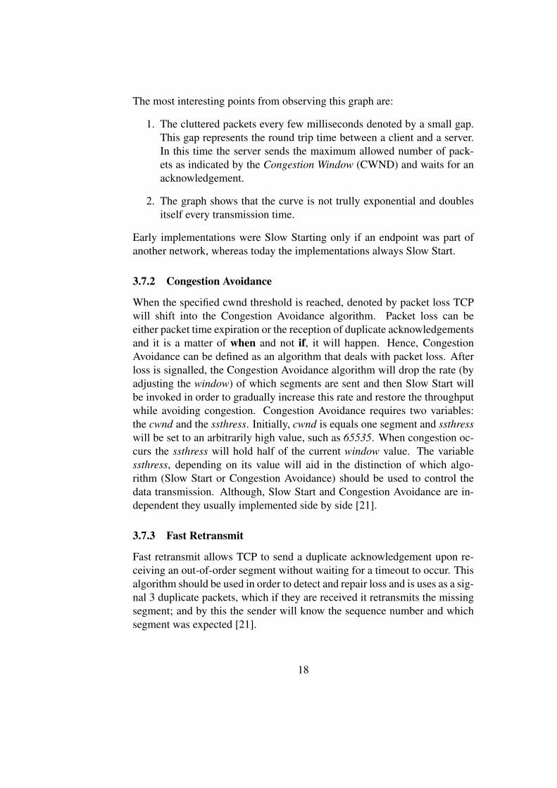
The most interesting points from observing this graph are:

1. The cluttered packets every few milliseconds denoted by a small gap.This gap represents the round trip time between a client and a server.In this time the server sends the maximum allowed number of pack-ets as indicated by the Congestion Window (CWND) and waits for anacknowledgement.

2. The graph shows that the curve is not trully exponential and doublesitself every transmission time.

Early implementations were Slow Starting only if an endpoint was part ofanother network, whereas today the implementations always Slow Start.

3.7.2 Congestion Avoidance

When the specified cwnd threshold is reached, denoted by packet loss TCPwill shift into the Congestion Avoidance algorithm. Packet loss can beeither packet time expiration or the reception of duplicate acknowledgementsand it is a matter of when and not if, it will happen. Hence, CongestionAvoidance can be defined as an algorithm that deals with packet loss. Afterloss is signalled, the Congestion Avoidance algorithm will drop the rate (byadjusting the window) of which segments are sent and then Slow Start willbe invoked in order to gradually increase this rate and restore the throughputwhile avoiding congestion. Congestion Avoidance requires two variables:the cwnd and the ssthress. Initially, cwnd is equals one segment and ssthresswill be set to an arbitrarily high value, such as 65535. When congestion oc-curs the ssthress will hold half of the current window value. The variablessthress, depending on its value will aid in the distinction of which algo-rithm (Slow Start or Congestion Avoidance) should be used to control thedata transmission. Although, Slow Start and Congestion Avoidance are in-dependent they usually implemented side by side [21].

3.7.3 Fast Retransmit

Fast retransmit allows TCP to send a duplicate acknowledgement upon re-ceiving an out-of-order segment without waiting for a timeout to occur. Thisalgorithm should be used in order to detect and repair loss and is uses as a sig-nal 3 duplicate packets, which if they are received it retransmits the missingsegment; and by this the sender will know the sequence number and whichsegment was expected [21].

18

3.7.4 Fast Recovery

After Fast Retransmit finishes resenting a lost datagram, fast recovery is tak-ing over until there are no more duplicate packets. In other words, Conges-tion Avoidance will be invoked right after Fast Retransmit but without SlowStart for increased performance, mainly due to that duplicate acknowledge-ments denote out-of-order datagrams and the rate can be increased fasterthan congestion occurs [21]. It is worth noting that Fast Retransmit and FastRecovery are usually implemented together.

3.7.5 Taxonomy of TCP Congestion Control algorithms

As stated before, TCP Congestion Control is an integral and important partof TCP and its performance; a good congestion control algorithm utilises thenetwork’s bandwidth, while mitigating potential packet losses. TCP Conges-tion Control, according to what it was developed to consider as congestion,could be categorised into: loss-, delay- and hybrid- based algorithms.

• Loss-based – Considers packet loss as a network congestion symptomand reduces the congestion window (cwnd), when packet loss occursor increases it otherwise.

• Delay-based – Considers as a symptom of network congestion thequeuing delay or in other words the actual time a packet requires inorder to be transmitted from the sender to the receiver.

• Hybrid-based – Considers both delay and loss a network congestionsymptom.

3.8 Evaluation Criteria

To evaluate the routing protocols, one can choose many different metrics;in this report the following metrics will be considered: throughput, routingoverhead, packet delivery ratio and end-to-end delay. Those metrics werechosen as they are the most common metrics used to evaluate the perfor-mance of networks and they are used by many researchers, for instance in[4] and [5], which make them ideal candidates as they are really understoodmetrics with readily available information. A description of the chosen met-rics follows in order to facilitate the reader.

19

3.8.1 Throughput

Throughput is the average rate of delivering successfully a packet (or mes-sage) over a communication channel which could be Ethernet, radio, etc.Throughput is usually being measured depending on context as bits per sec-ond (bps), or data packets per second or data packets per time slot. Throught-put is a very important metric for a network and its value should be as highas possible.

3.8.2 Packet Delivery Ratio

The result of the computation of the successfully delivered packets to a des-tination, by the number of packets sent. The greater this figure is, the better arouting protocol performs. A general formula for calculating packet deliveryratio as a percentage is as follows:∑

packets_received∑packets_sent

x100

3.8.3 Routing Overhead

Routing overhead is the sum of all routing packets. Routing packets meanall the packets send by a source, in order to find a destination node or in-form about link failures. Routing overhead has an immediate impact on anetwork’s scalability; it is usually measured in bits per second, or packetsper second. As a result, when a network expands its routing traffic increasesas well.

3.8.4 End-to-End delay

End-to-End delay is the amount of time required for a packet to travel fromthe source until it reaches its destination. Typically, it can be calculated by:∑

(arrival_time− sent_time)∑number_of_connections

The most common measurement unit is milliseconds and it is really impor-tant, depending on the use of a network, for this value to be small. In regardsto routing protocols the smaller the end to end delay is the better a protocolis perfoming. For instance, the International Telecommunication Unit (ITU)recommends in a Packet Voice network with adequetly handled echo or inother words with echo cancellers utilised, the following one-way delays[22]:

20

Milliseconds Comment0-150 All users are satisfied.

150-400 Some users will be dissatisfied.400 and above Unacceptable for general network planning purposes.

However there might be some exceptional cases.

Table 3.2: ITU One-way delay recommendation

21

4 Implementation of TCP Congestion Control Mechanisms

In this chapter, the reader will be given a short introduction to the implemen-tation of TCP-FIT and TCP-Illinois.Both TCP-FIT and TCP-Illinois, have been developed for wireless networkswhich are subject to challenging network conditions. As a result, they areexpected to function and achieve better results over mechanisms that are de-veloped for wired networks.

4.1 Development Environment

The development environment for the implementation is OMNeT++[8] it-self. OMNeT++ IDE is based on the Eclipse platform, which is strippedfrom all Java related development tools. This allows the size distribution tobe small, and any developer to make his/her own plugins for the frameworkthrough the extensible plugin system of Eclipse.OMNeT++ contains the following tools pre-installed [23]:

• All OMNeT++ specific tools you use such as NED, MSG and INI fileeditor, result analysis tools, documentation generator etc.

• The C/C++ Development Tooling (CDT), used for C++ developmentand debugging, which further integrates with the standard gcc toolchainand the gdb debugger.

4.1.1 OMNeT++

OMNeT++ [8] is a C++ based discrete event simulation environment de-veloped for modelling networks, multiprocessors, etc. It operates under theAcademic Public License, which makes the software free for non-profit use.OMNeT++ recognition as a platform for simulating networks and distributedsystems among the Academic Community and researchers is rising. OM-NeT++ in its core is following a framework-wise philosophy and providesjust the necessary mechanisms and tools to the user in order to write simula-tions or create his own simulator.In other words, OMNeT++ can be seen as a platform for simulating computernetworks and distributed systems, meaning that OMNeT++ is not a simulatorand it merely provides the necessary infrastructure for writing simulations.Depending on the application area or problem domain a researcher can utiliseother frameworks like INET and VEINS through OMNeT++ and build hisown simulation environment.

22

4.1.2 INET Framework

The INET framework was built as an extension model library to OMNeT++.It provides to OMNeT++ a set of agents, protocols, models for the InternetSuite, such as TCP, UDP, IPv4, BGP, etc. Moreover, it has also mobility sup-port and wireless radio communication and distribution models along withseveral implementations of MAC protocols, and a lot of other useful features,which make INET ideal for students and researchers of communication net-works [24].

INET above all is open-source and many of its components have theirown licences (either LGPL or GPL). INET is well-supported and commu-nity driven. At the moment of writing, the developers of INET are incorpo-rating most of the features found in MiXiM framework, but lacking or wereincomplete in INET. This will result in more meaningful environment im-plementations with objects, better environment control etc. As OMNeT++,INET is following the logic of modules, which one can simply put togetherand create a “realistic” scenario.

4.1.3 Modelling a simulation

A simulation in OMNeT++ can be seen as a structure of independent butclosely related modules, which communicate by message passing and to-gether they form an OMNeT++ model. The equivalent is to think of thosemodules as LEGO pieces, which should you combine them; you obtain atruly unique item with specific characteristics. Modules can be categorisedas simple modules or compound modules, where compound modules are agroup of simple modules. This idea is illustrated in Figure 4.1.

Figure 4.1: Module Structure in OMNeT++

23

For instance, to measure in this report the throughput of the network, themodule NodeBase was extended and used as its basis the StandardHost mod-ule implementation, which was modified further to include two Thruput-Meter modules. It is required to use two ThruputMeter modules in orderto collect both incoming and outgoing traffic.

To evaluate the throughput of the TCP protocol it is required to placethe ThruputMeter modules between the TCPApp (Application Layer) andthe TCP layer. This is a key step, as TCP, due to its nature will generatemany packets for its operation after the TCP layer, in response to out of or-der deliveries, lost packets, acknowledgements (duplicate or not) etc. andthis will produce false measurements. In networking terms, when the appli-cation level data is being measured, it is called more accurately goodput. Themodification is shown in Figure 4.2 (surrounded in red):

Figure 4.2: Modified Mesh Node with 2 thruputMeters

There has been other modifications at the source of several components suchas TCPSessionApp, Batman protocol and others, see github [10].

Furthermore, OMNeT++ provides the user with a complete GraphicalUser Interface, which allows the person, who runs the simulation, to havea complete view of the simulation internals; it shows the network topologyand graphics, it displays the message flow between the different componentsas an animation, and at any given moment a user can peek inside the compo-

24

nents and variables, like for instance, to determine if a routing table is as itshould [23].A simulation is formed by the following parts [23]:

1. The Network, which is a file or files that describe the structure of sim-ple or compound modules along with their parameters, gates, channelsetc. This file is written using the NED language.

2. A definition of the message types and data structures, which OM-NeT++ will do the necessary translation into C++ equivalent classes.These definitions come with the .msg extension.

3. The Modules, the actual implementation of the modules, done in C++and usually have the suffix .cc. A module can be a router, an HTTPserver or in a more general sense anything that has networking capa-bilities and can be connected in a network.

4. The gates, which are the connection end-points of the modules. Thereare three types of gates: input, output and inout.

The steps required to create a new project in OMNeT++/INET are describedin Appendix 2.

4.2 TCP Congestion Flavours in OMNET++/INET

The INET Framework provides several implementations of TCP CongestionControl Mechanisms, including TCP Westwood which targeting wirelessnetworks, all can be found under the directory src>inet>transportlayer>tcp>flavours. In order to implement a TCP Congestion flavour in INET, a spe-cific structure needs to be followed. Classes should extend the functionalityof TCPBaseAlg, which itself is an extension of the TCPAlgorithm class andoverride some or all of the provided methods, should different behaviour isrequired. For a brief reference some of the methods one can override are:

• dataSent(uint32 fromseq) - Invoked after data was sent. This hook canbe used to schedule the retransmission timer, to start round-trip timemeasurement, etc. The argument is the seqno of the first byte sent.

• segmentRetransmitted(uint32 fromseq, uint32 toseq) - Called after aretransmitted segment. The argument fromseq is the seqno of the firstbyte sent. The argument toseq is the seqno of the last byte sent+1.

25

• receivedDuplicateAck() - Per class documentation, this method will beinvoked after a received duplicate ACK (that is: ackNo == snd_una, nodata in segment, segment there is unacked data). The dupack countergot already updated when calling this method (i.e. dupacks == 1 onfirst duplicate ACK.)

4.3 Overview of TCP-FIT

TCP-FIT is a hybrid congestion control network mechanism, which consid-ers both delay and packet loss as a signal for congestion. For its implementa-tion an article describing the algorithm’s pseudocode [25] along with severalother important properties was used.

4.3.1 Keypoints on the implementation

• TCP-Fit is using the same mechanisms for Fast-Retransmit and FastRecovery as TCP-Reno.

• The pseudocode provided was implemented as is, and by following theseveral hints, from the authors in the paper.

• TCP-Fit, now TCP-Max, is following a commercialisation path and assuch, there is a possibility that the authors did not disclose modifica-tions to the mechanisms of TCP-Reno or others, which might producebetter results.

4.4 Overview of TCP-Illinois

TCP-Illinois is also a hybrid congestion control algorithm. It is using packetlosses as a way to determine, whether the congestion window should be in-creased or decreased; and queueing delay to determine how much the amountof increment or decrement should be.

TCP-Illinois is an algorithm developed to achieve high throughput, andfairly utilise network resources. Further, TCP-Illinois is also highly compat-ible with the TCP standard [26]. TCP-Illinois is already implemented intothe Linux kernel and it was used as a guide for implementing/porting TCP-Illinois to OMNeT++/INET.

4.4.1 Keypoints on the implementation

• The source code of the linux implementation of TCP-Illinois [27] wasused as a guide to port the algorithm into OMNET++/INET.

26

• There have been only minor changes in the code, which do not affectthe performance, but allows the algorithm to function insideOMNET++/INET.

4.5 Congestion Windows for both algorithms after implementation.

In this chapter a comparison will be drawn, between the graphs producedfrom the tests run in this report, and those of the authors for both algorithms.

The scenario tcpclientserver provided with the INET examples was used,as it is a simple TCP Client-Server scenario where the client is sending 50megabytes to a server through a wired connection, which allows smooth re-sults with minimal packet collisions.

Figure 4.3: CWND of TCP-Illinois and TCP-Fit (our testing)

27

Figure 4.4: CWND of TCP-Illinois (in blue) top, and TCP-Fit bottom, asmeasured by the their creators.

The similaries are clearly visible, and at this point it is considered that the im-plementation reached its final phase. The source code of the implementationis provided through GitHub [10]under the LGPL licence; further researchand refinement of the source is encouraged.

28

5 Results

This chapter presents and discusses the results of the different scenarios forUDP and TCP.

5.1 Scenario structure for collecting data

The results will be presented by their performances namely the routing over-head, the end-to-end delay, the goodput and finally by the packet deliveryratio. Also in the TCP results the Round Trip Time will be discussed butwill not be taken into serious consideration as some of the connected clients(TCP Sess.) did not produce any data recordings.

Scenario CommentUDP DYMO & BATMAN 5 clients static, walking and drivingUDP DYMO & BATMAN 15 clients static, walking and drivingTCP-NewReno DYMO 5 clients static, walking and drivingTCP-NewReno BATMAN 5 clients static, walking and drivingTCP-Illinois DYMO 5 clients static, walking and drivingTCP-Illinois BATMAN 5 clients static, walking and drivingTCP-FIT DYMO 5 clients static, walking and drivingTCP-FIT BATMAN 5 clients static, walking and drivingTCP-NewReno DYMO 15 clients static, walking and drivingTCP-NewReno BATMAN 15 clients static, walking and drivingTCP-Illinois DYMO 15 clients static, walking and drivingTCP-Illinois BATMAN 15 clients static, walking and drivingTCP-FIT DYMO 15 clients static, walking and drivingTCP-FIT BATMAN 15 clients static, walking and driving

Table 5.1: Scenarios run to accumulate the data.

Table 5.1, lists in brief all the different scenarios that were considered andrun, in order to accumulate the data that will serve as the basis of our analysis.More scenarios could be run with more clients, however, that was not pos-sible due to resources limitation. Resources limitation is this context meansthe laptop, where the scenarios were run on, was not powerful enough to ac-comodate larger networks and more clients. To review most of the settingsused in the scenarios, refer to Appendix 1. Furthermore, many recordingstatistics were disabled as they were not very relevant, were slowing downour simulations and lastly requiring a really large amount of space, that wasnot available at the moment.

29

5.2 UDP Results

Figure 5.1, describes the results accumulated after all the UDP scenarioswere concluded. The blue bars in the figure describe the scenarios with 5clients, whereas the red bars the scenarios with 15 clients. Furthermore,the bottom axis is named after the protocol and the scenario as such proto-col_scenario. For instance BATMAN_S means BATMAN as routing proto-col and static (S) scenario. For complicity W means Walking and D driving.

30

Figure 5.1: UDP results for B.A.T.M.A.N. and DYMO

31

5.2.1 Routing overhead

According to the data collected in Figure 5.1, the B.A.T.M.A.N. protocoltransmits the highest amount of routing traffic in the network, followed byDYMO, which transmits the least. This is true for all the scenarios testedwith either 5 or 15 traffic sources in static, walking and driving scenarios.

Hence, in terms of routing overhead DYMO, outperforms B.A.T.M.A.Nand in the case of a network with low resource requirements, DYMO wouldbe a better choice as it would perform better.

5.2.2 End-To-End delay

It was observed that B.A.T.M.A.N. has the lowest end-to-end delay com-pared to DYMO in all scenarios with 5 traffic sources. When the trafficsources increase and mobility is introduced, B.A.T.M.A.N’s delay perfor-mance competes with that of DYMO.

B.A.T.M.A.N manages to maintain a quite stable end-to-end delay andperforms much better than DYMO in all scenarios, even with higher mobilityspeeds.

5.2.3 Goodput

From Figure 5.1, B.A.T.M.A.N. in the static and walking scenarios with 5clients record a higher goodput, which as was mentioned earlier, is an indi-cator that a protocol performs better over others or in our case it performsbetter than DYMO.


DYMO is following B.A.T.M.A.N. in both static and walking scenarios with5 clients, which has a higher packet delivery ratio. In the driving scenarioB.A.T.M.A.N. performs poorly, whereas DYMO even though it is affectedby the higher speeds, still performs better with a PDR of approximately 60%.

On the other hand, when the clients (traffic sources) are increased, DYMOhas a highest packet delivery ratio than B.A.T.M.A.N. and consequently out-performs it.

32

5.3 TCP Results (static scenario)

Table 5.2 describes the data collected from the TCP static scenario with allTCP variants. The first column is the scenario run, the second is the mea-sured goodput, the third is the packet delivery ratio (PDR), the fourth is av-erage mean round trip time, the fifth the routing overhead and lastly the TCPSessions.

There are two columns that reserve explanation, the Average mean RTT,which is the sum of the mean round trip times values recorded from theclients and then divided by the number of the recorded values; and the TCPSession, which represents how many clients managed to connect with thegateway.

TCP NewRenoStatic Scenario Goodput (bits/s) PDR Avg. mean RTT OHD TCP Sess.

DYMO 5 Clients 721267 21.6% 0.0246923 146844 5

DYMO 15 Clients 4824574 48.2% 0.0276579 267236 14

BATMAN 5 Clients 3114560 93.4% 0.0245930 764079 5

BATMAN 15 Clients 5388584 67.4% 0.0165166 1285406 12

TCP IllinoisStatic Scenario Goodput (bits/s) PDR Avg. mean RTT OHD TCP Sess.

DYMO 5 Clients 783953 23.5% 0.0021406 144912 5

DYMO 15 Clients 4931707 56.9% 0.0032317 232622 13

BATMAN 5 Clients 3333332 100.0% 0.0021237 769403 5

BATMAN 15 Clients 5980280 64.1% 0.0028525 1279475 14

TCP FitStatic Scenario Goodput (bits/s) PDR Avg. mean RTT OHD TCP Sess.

DYMO 5 Clients 855865 25.7% 0.0031685 139497 5

DYMO 15 Clients 4876583 52.2% 0.0044332 233472 14

BATMAN 5 Clients 3333332 100.0% 0.0042324 765245 5

BATMAN 15 Clients 5888196 63.1% 0.0038250 1285407 14

Table 5.2: Results from the TCP static scenario.

5.3.1 Round Trip Time (RTT)

DYMO and TCP-Newreno keep the RTT inside acceptable limits. However,B.A.T.M.A.N. performs better with slightly lower RTT, around 0.4021%decrease with 5 clients, and a much lower decrease of 40.2825% with 15

33

clients. The same is observed with TCP-Illinois, B.A.T.M.A.N. records a0.7895% decrease in RTT with 5 clients and 11.7338% with 15 clients.With TCP-FIT and 5 clients DYMO performs better with 25.137% decreaseover B.A.T.M.A.N., which records a lower RTT with 15 clients of around13.7192%.

The round trip time between the TCP variants, show that TCP-FIT andTCP-Illinois have a much smaller RTT than TCP-Newreno, which also resultin a better goodput. Also B.A.T.M.A.N. outperforms DYMO by having alower RTT in most of the scenarios.

5.3.2 Goodput

The developers from both TCP-FIT and TCP-Illinois promised in their corre-sponding papers a higher throughput, which is reflected in the obtained dataand results in a higher goodput.

B.A.T.M.A.N. shows an increase of 331.8179% in goodput with 5 clientsand TCP-Newreno and 11.6904% with 15 clients. 325.1954% increase with5 clients and 21.2619% with 15 clients and TCP-Illinois as the algorithm.With TCP-FIT and increase of 289.4694% in the goodput for B.A.T.M.A.N.with 5 clients and 20.7443% with 15 clients. As a result, B.A.T.M.A.N.outperforms DYMO with every algorithm.


The packet delivery ratio (PDR) observed shows the TCP-FIT and TCP-Illinois outperforms TCP-Newreno. However, with 15 clients and B.A.T.M.A.N.as the routing protocol, TCP-Newreno shows better PDR. Also, B.A.T.M.A.N.performs better than DYMO.


It is worth noting that when comparing TCP-Illinois and TCP-FIT with TCP-Newreno, the former two show a reduction in the overall routing overhead forboth routing protocols. B.A.T.M.A.N. as a proactive protocol is performingpoorly over DYMO.

34

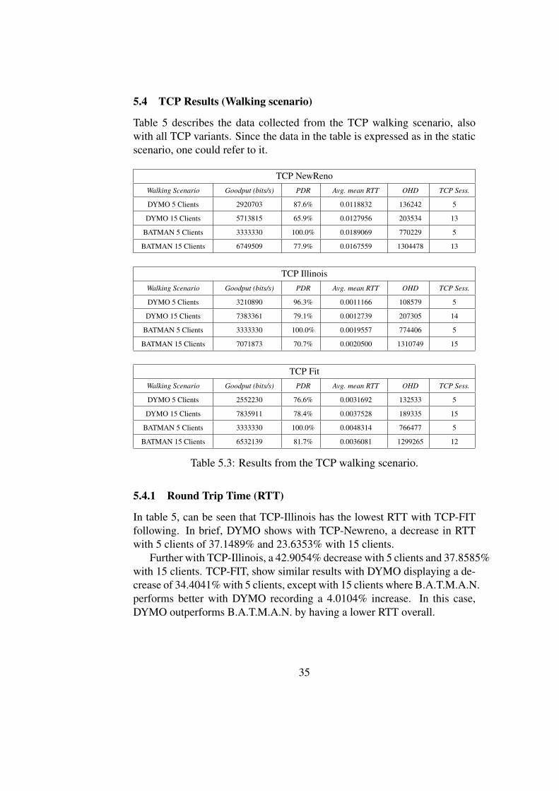
5.4 TCP Results (Walking scenario)

Table 5 describes the data collected from the TCP walking scenario, alsowith all TCP variants. Since the data in the table is expressed as in the staticscenario, one could refer to it.

TCP NewRenoWalking Scenario Goodput (bits/s) PDR Avg. mean RTT OHD TCP Sess.

DYMO 5 Clients 2920703 87.6% 0.0118832 136242 5

DYMO 15 Clients 5713815 65.9% 0.0127956 203534 13

BATMAN 5 Clients 3333330 100.0% 0.0189069 770229 5

BATMAN 15 Clients 6749509 77.9% 0.0167559 1304478 13

TCP IllinoisWalking Scenario Goodput (bits/s) PDR Avg. mean RTT OHD TCP Sess.

DYMO 5 Clients 3210890 96.3% 0.0011166 108579 5

DYMO 15 Clients 7383361 79.1% 0.0012739 207305 14

BATMAN 5 Clients 3333330 100.0% 0.0019557 774406 5

BATMAN 15 Clients 7071873 70.7% 0.0020500 1310749 15

TCP FitWalking Scenario Goodput (bits/s) PDR Avg. mean RTT OHD TCP Sess.

DYMO 5 Clients 2552230 76.6% 0.0031692 132533 5

DYMO 15 Clients 7835911 78.4% 0.0037528 189335 15

BATMAN 5 Clients 3333330 100.0% 0.0048314 766477 5

BATMAN 15 Clients 6532139 81.7% 0.0036081 1299265 12

Table 5.3: Results from the TCP walking scenario.


In table 5, can be seen that TCP-Illinois has the lowest RTT with TCP-FITfollowing. In brief, DYMO shows with TCP-Newreno, a decrease in RTTwith 5 clients of 37.1489% and 23.6353% with 15 clients.

Further with TCP-Illinois, a 42.9054% decrease with 5 clients and 37.8585%with 15 clients. TCP-FIT, show similar results with DYMO displaying a de-crease of 34.4041% with 5 clients, except with 15 clients where B.A.T.M.A.N.performs better with DYMO recording a 4.0104% increase. In this case,DYMO outperforms B.A.T.M.A.N. by having a lower RTT overall.

35

5.4.2 Goodput

TCP-Illinois seems to perform much better and give a higher goodput whencompared to the other two TCP variants. TCP-FIT is following with similarresults.

With TCP-Newreno, B.A.T.M.A.N. has an increase of 14.1277% with5 clients and a 18.1261% with 15 clients. With 5 clients and TCP-Illinois,B.A.T.M.A.N. is showing a small increase of 3.8133% and a decrease of4.2188% with 15 clients. 30.6046% increase with 5 clients and TCP-FITand 16.6384% decrease with 15 clients.

B.A.T.M.A.N. seems to perform better, except in the cases with TCP-Illinois and TCP-FIT with 15 clients.


TCP-Illinois and TCP-FIT have a higher PDR than TCP-Newreno. Further,both routing protocols perform equally well with TCP-Illinois and TCP-FIT,since there are a few TCP sessions less, in some scenarios.


In table 5, TCP-FIT records low values for routing overhead in all but onescenario and such is winning at this measurement with surprisingly TCP-Newreno following. Also, as expected DYMO is outperforming B.A.T.M.A.N..

36

5.5 TCP Results (driving scenario)

The data collected from the TCP driving scenario with all TCP variants isdescribed by table 6 in a similar fashion as in the static scenario, which onecould refer to.

TCP NewRenoDriving Scenario Goodput (bits/s) PDR Avg. mean RTT OHD TCP Sess.

DYMO 5 Clients 1529055 45.9% 0.0254553 259569 5

DYMO 15 Clients 6016713 64.5% 0.0108939 398989 14

BATMAN 5 Clients 77167 2.3% 0.0449272 1371442 5

BATMAN 15 Clients 3460127 34.6% 0.0218555 2087110 15

TCP IllinoisDriving Scenario Goodput (bits/s) PDR Avg. mean RTT OHD TCP Sess.

DYMO 5 Clients 1583725 47.5% 0.0020532 254529 5

DYMO 15 Clients 5830933 62.5% 0.0010029 384607 14

BATMAN 5 Clients 142956 5.4% 0.0024014 1369909 4

BATMAN 15 Clients 3712318 39.8% 0.0029375 2076197 14

TCP FitDriving Scenario Goodput (bits/s) PDR Avg. mean RTT OHD TCP Sess.

DYMO 5 Clients 1579903 47.4% 0.0030182 257512 5

DYMO 15 Clients 6635451 66.4% 0.0027660 386345 15

BATMAN 5 Clients 98290 3.7% 0.0096568 1370718 4

BATMAN 15 Clients 3843335 44.3% 0.0062592 2079371 13

Table 5.4: Results from the TCP driving scenario.


TCP-Illinois is outperforming the other variants in this scenario with TCP-FIT following and TCP-Newreno being far behind. Regarding the routingprotocols DYMO outperforms B.A.T.M.A.N. in all scenarios by a decreaseof 43.34% with 5 clients and a decrease of 50.15% with 15 clients.

DYMO and TCP-Illinois record a decrease of 14.5% with 5 clients andwith 15 clients a decrease of 65.86%. With TCP-FIT and 5 clients and 15clients, a decrease of 68.75% and 55.81%, respectivelly.

37

5.5.2 Goodput

TCP-FIT and TCP-Illinois seem to outperform TCP-Newreno and recordhigher goodput with the exception the difference between TCP-Newreno andTCP-Illinois with DYMO as the protocol and 15 traffic sources, where TCP-Illinois is not performing as good as TCP-Newreno. DYMO also outper-forms B.A.T.M.A.N. an increase of 1881.49% and 73.89% with 5 and 15clients respectively.

With an increase of 1007.84% with 5 traffic sources and 57.07% with 15traffic sources with TCP-Illinois. Lastly, with TCP-FIT records an increaseof 1507.39% and 72.65%.


Table 4, shows that TCP-FIT would outperform all other TCP variants in allbut one scenario, however, the amount of clients connected does not give aclear and definitive answer. TCP-Newreno seems to also perform and handlethe higher mobility equally well. DYMO clearly from the table performsbetter than B.A.T.M.A.N..


TCP-FIT and TCP-Illinois record lower values for routing overhead in allscenarios. As expected, DYMO records the lowest routing overhead andoutperforms B.A.T.M.A.N..

5.6 TCP Goodput change

Table 7 lists the change of the goodput in the form of percentage, and it wascreated in an effort to display the goodput difference between the congestioncontrol algorithms tested in this report.

The reason for its creation was mainly the fact that all congestion con-troll algorithms developed for wireless networks promise an increase in thethroughput, which consequently results in an increase in goodput. A negativenumber in the table means an algorithm performed worst.

38

Goodput change in Static scenarios (percentage)Scenario Illinois vs. NewReno FIT vs. NewReno FIT vs. Illinois

DYMO 5 Clients 8.69% 18.66% 9.17%DYMO 15 Clients 2.22% 1.08% -1.12%

BATMAN 5 Clients 7.02% 7.02% 0.00%BATMAN 15 Clients 10.98% 9.27% -1.54%

Goodput change in Walking scenarios (percentage)Scenario Illinois vs. NewReno FIT vs. NewReno FIT vs. Illinois

DYMO 5 Clients 9.94% -12.62% -20.51%DYMO 15 Clients 29.22% 37.14% 6.13%

BATMAN 5 Clients 0.00% 0.00% 0.00%BATMAN 15 Clients 4.78% -3.22% -7.63%

Goodput change in Driving scenarios (percentage)Scenario Illinois vs. NewReno FIT vs. NewReno FIT vs. Illinois

DYMO 5 Clients 3.58% 3.33% -0.24%DYMO 15 Clients -3.09% 10.28% 13.80%

BATMAN 5 Clients 85.26% 27.37% -31.24%BATMAN 15 Clients 7.29% 11.07% 3.53%

Table 5.5: Goodput differences between the TCP variants. A negative num-ber means an algorithm performed not as well.

39

6 Discussion

In this chapter the report’s discussion is drawn.In this section the problems that occured during the implementation of

the two congestion control algorithms will be discussed. Followed by a dis-cussion on the configuration and lastly on the different results.

6.1 Problems during the implementation of congestion control mecha-nisms.

During the implementation of the two TCP congestion algorithms there werenumerous problems encountered, that needed to be resolved before proceed-ing further. Those problems were mostly related, either with the implementa-tion itself or in the case of TCP-Illinois with understanding the Linux kernelimplementation of the algorithm.

6.1.1 Issues with the kernel implementation

In brevity, in the Linux kernel implementation there were some methodsalong with their parameters that lack any further explanation. Hence, anunderstanding of how different methods, parts and internal TCP functionswork needed to be done. After reading numerous fragments of informationregarding kernel patches, and the source codes of existing implementationsin the INET framework, a picture was drawn and the implementation wentfurther. In its final state only some variables were changed, which do notaffect the algorithm’s performance, and allow it to run in OMNET++/INET.For instance, one such small change was the current timestamp, which waschanged to OMNET++ simulation time.

6.1.2 TCP-FIT algorithm considerations

TCP-FIT, although not widely used or adopted, its algorithm is given in pseu-docode form, in[25] where the algorithm is described. In this paper there areseveral suggestions that were taken into consideration. One of them is theupdate interval (update_epoch) of the algorithm, which was set to 500 ms,as the developers did in their testing. However, due to that this value canproduce different results, it worths more investigation. Another suggestion isthe use of a slightly different formula, considering the beta value, which wasadded in the code and can be used, when the user provides a different valuefor beta and then re-compile the code.

40

Furthermore, the TCP-FIT algorithm’s implementation provided [10] mightnot be absolutely correct as the developers are following a commercialisedapproach and their pseudocode describes only the algorithm’s internals, andskips the fast-recovery and fast re-transmitt parts, by mentioning only thatthey are similar to TCP-Reno that the algorithm tries to improve. As a result,those mechanisms were kept as is from TCP-Reno.

6.1.3 Modifications into OMNET++/INET nodes

To retrieve the required results some files needed to be changed, like thethruputmeter, batman protocol and some tcp files. All these files are providedin the same github directory as the algorithms [10].

Nevertheless, both algorithms reached their final state for this report. Theresults from several tests seem to give satisfactory results and as such, thealgorithms are freely available under the LGPL license in github [10].

6.2 Configuration

Concerning the obtained results, it is worth mentioning that all the scenarioswere not set in an ideal world without noise and interference, and it is alsoworth noting that this fact is what affects the performance of both routingprotocols in all the scenarios, and mostly those with 15 clients and thosewith mobility. In other words, in a moderate mobility scenario, due the clientmovement the interference, the noise and the possible packet collisions areminimised as the clients move and give space to others. The opposite istrue with 15 or more clients where the network becomes crowded and theperformance worsens.

In this report,both UDP and TCP nodes were configured as such: in theUDP scenarios the message length was set to 1024 bytes (1MB), the clientswere set to send packets in one second burst with a slightly variable interval,which produces every second either heavy or medium traffic. Moreover, inthe UDP configuration the sleep and the stop time were disabled, meaningthat data will be sent at once, and the clients will keep sending data as longas the simulation runs. TCP proved a little trickier due to bigger amountof settings it needs. Nevertheless, most of the TCP features remained attheir default values with the exception of the advertised window, maximumsegment size and Nagle algorithm. The TCP clients were configured to makea connection with the gateway mesh station and each of them sent 300MB ofdata with a variable time of sending the data and opening the connection. Thevariable time for opening the connection and sending the data was chosen inan effort to mitigate collisions at the MAC layer or in other words to limit the

41

possibility of all clients trying to send data at the same time. What is more,another crucial factor in regards to the wireless receiver and transmitter of thenodes was the calibration of the contention window. The contention windowwas set according to the information found in several slides [28] and arespecific to wireless “g” mode. The values that worked best in this case andgave a higher packet delivery ratio were:

• slot time = 9us (default)

• Cwmin = 31, and

• Cwmax = 1023

The equivalent names of these settings in OMNET++/INET are cwMinData,cwMaxData and slotTime and all are part of the MAC layer of the wirelessdevice.

6.3 Results

6.3.1 UDP Overhead

Regarding the data obtained from the UDP results, the measured overheadis the total control packets sent from all involving nodes. In the case ofDYMO it also incorporates the routing error messages. Routing error mes-sages (RERR) are sent when a link or path towards a node fails. This messagepropagates itself to all nodes in the neighbourhood or vicinity of the node thatsends it. This is done in DYMO due to the lack of alternative routes towardsthe destination, as the routing table contains only the routes required and notall possible routes.

Nevertheless, it was expected that DYMO would outperform B.A.T.M.A.N.,since as it was described at chapter 3, on-demand or reactive routing proto-cols transmit control packets only when a source needs to send some data,which consequently reduces the routing overhead by not "polluting" the net-work with unnecessary routing traffic. Whereas proactive protocols likeB.A.T.M.A.N. always send control packets to monitor and maintain its rout-ing table.

In the considered simulations, the default interval of sending controlpackets was increased, 2 seconds from 1 for both B.A.T.M.A.N. and DYMO,as those numbers produced better results. Also it is important to mention,that by default DYMO relies on the link state information to discover faultsin the paths. This behaviour in the simulations resulted with poor perfor-mance and as such it was overridden by setting the sending interval of theHELLO messages.

42

6.3.2 UDP End-to-end delay

The measured end-to-end delay shows that B.A.T.M.A.N. outperforms DYMO.The reason behind this observation is that B.A.T.M.A.N. maintains a routingtable for every possible destination and has its routes ready for when dataneeds to be sent, unlike DYMO which always requests the route, if not in thetable or in case it was deleted, failed or changed.

6.3.3 UDP Routing overhead

DYMO recorded a lower routing overhead, as better seen in the results fromchapter 5. Since, DYMO is an on-demand routing protocol and this allowsthe protocol to be fairly consistent which despite the higher one-way delay(which is still inside acceptable limits), to have a much lower impact onthe network traffic by regulating its routing overhead by need (On-demand).Moreover, it performs also better in a driving scenario and it is worth notingthat in a highway or in a town, clients can also act as mesh stations andprovide many different network gateways (not visible with our simulations),which might or might not allow for better performance or different results.

6.3.4 UDP Goodput

The results show that B.A.T.M.A.N. records a higher goodput and this canbe explained as proactive protocols already know which path to follow toreach a destination, and since throughput (goodput is always less) is definedas the total amount of data received to the time the receiver got the very lastpacket. As a result B.A.T.M.A.N. which has lower delay in those scenarioshas a higher goodput.

Moreover, as the traffic sources are increased the routing protocols haveto work harder to compensate with network degradation, and problems likecongestion, hidden terminals, etc. In the results, this is visible as B.A.T.M.A.N.displays higher delay, which results in a much lower goodput. This meansthat while the network is small and the mobility is low or completely static,B.A.T.M.A.N. outperforms DYMO. However, as the network grows whetherthere is mobility or not, the opposite is true.

6.3.5 TCP

On the other hand, from the TCP results it was observed that TCP congestionalgorithms designed for wireless networks can offer greater performance.

43

6.3.6 TCP Static scenarios

In brief, from the static scenarios it became clear that congestion controlalgorithms designed for wireless networks perform much better and give aspromised a higher throughput.

Regarding the Round Trip Time (RTT), TCP-Illinois seems to outper-form the other two algorithms with TCP-FIT following. This is visible inour results with TCP -FIT and -Illinois having a similar performance. How-ever, the similarities could be due to the number of the connected clients (asindicated by the TCP Sess. column).

According to this column, only 12 out of 15 clients managed to connect,which might be the reason for such differences during the simulation’s run-ning time. In other words, the smaller amount of connected clients recordmore data in the simulation’s time, whereas in the other TCP variants the re-sults show less packets sent, which is due to more collisions, re-transmittions,congestion etc. Nevertheless, TCP-FIT and TCP-Illinois seem to performbetter in wireless networks.

In any case, a proactive protocol like B.A.T.M.A.N. seems to performbetter than DYMO in the static scenarios, which was as expected, since TCP,unlike UDP, in order to operate needs a stable route as it is an end-to-end con-nection oriented communication protocol. The most strange results are withDYMO and 5 clients, as it was expected to perform as well as B.A.T.M.A.N.,that did not happen and a satisfactory explanation was never found. A spec-ulation could be that, on-demand routing and the various TCP timers foracknowledgements. etc. which had a negative impact on DYMO’s perfor-mance.

6.3.7 TCP Walking scenarios

In the walking scenarios, the recorded difference is due to how many clientswere connected and how they were moving. Like the UDP scenarios, withmoderate mobility the routing protocols and the TCP congestion control al-gorithm perform better, for similar reasons. Despite that TCP-Illinois seemedsuperior in most scenarios, the performance of TCP-FIT cannot be neglectedand is it would be good to note, that it seems to be able to perform better thanTCP-Newreno.

Regarding the packet delivery ratio in the walking scenarios, it wouldbe safe to say that according to the number of clients connected, both TCP-Illinois and TCP-FIT record very similar results, and should the clients con-nected were the same amount, we would probably have same results. Wecould only say that the TCP-Illinois is a better algorithm, due to the number

44

of clients connected and that it outperformed TCP-Newreno.Overall in the walking scenarios, the results show that TCP-Illinois for

both routing protocols performs much better than TCP-Newreno, which is acongestion control mechanism designed for wired networks. Moreover, al-though TCP-Illinois and TCP-FIT are giving very similar results, the formeris winning the battle mainly due to that most of the clients were connectedwith the gateway node (TCP Sess.), with the latter being very close behind.From the results, is it worth noting that with TCP-FIT there is a reduction onthe overall routing overhead for both protocols.

6.3.8 TCP Driving scenarios

From the data collected from the driving scenarios, it can be observed that,like UDP, on-demand routing protocols can perform better under frequentrouting changes. All three TCP variants with DYMO give similar resultswith the only difference the increase in Goodput in both TCP-Illinois andTCP-FIT, which is as expected, since the developers of the algorithms hadin mind to provide better throughput. Better throughput, means an increasein Goodput as well, although slightly less than throughput due to TCP re-transmissions.

In the driving scenario both TCP-Illinois and TCP-FIT reduce the overallrouting overhead. To conclude, all TCP variants seem to perform well andgive similar packet delivery ratios in higher mobility scenarios, which mightbe due to the client movement the congestion is not reaching critical levels.Further, DYMO is clearly outperforms B.A.T.M.A.N. as expected.

6.3.9 Protocol comparison conclusion

Overall, it cannot be said with certainty that one routing protocol is the bestor the worst for a specific case. It would be up to the network designer totake the right decisions regarding a Wireless Mesh Network. For instance,if there is moderate mobility and the extra traffic generated by a proactiveprotocol is not causing any problems, one can choose that instead of another.

From the UDP results it can be observed that on-demand protocols in oursimulation seem to be more stable, and to perform better in the majority ofthe considered scenarios and environments, and it would be safe to say thatthey can come first in the order of preference. This is especially true whenthe network requires low resources, where on-demand protocols with theirlow routing overhead, should be the first choice or among the first.

Regarding B.A.T.M.A.N., it seems to perform better in static and moder-ate mobility scenarios, like walking, with very low one-way delays, except

45

the case when the number of the traffic sources increases, and their one-waydelay is competing with that of DYMO. To conclude, some of the facts thatone needs considering before choosing a proactive protocol, are:

1. The higher routing overhead.

2. Under frequent route changes, their performance may worsen and,

3. The routing tables as the network grows might grow fairly large, andwhen combined with all the problems in wireless networks, the net-work quality will degrade.

The TCP scenarios revealed, that congestion control algorithms should notbe neglected and a proper one must be chosen, as they can offer better per-formance in conjunction with the chosen routing protocol.

46

7 Conclusion

In this final chapter the report conclusion will be drawn.In this thesis two routing protocols for Wireless Mesh Networks were

compared in a set of scenarios that utilised two transport protocols, namelyUDP and TCP.When TCP is being used there are many congestion control variances thatcan improve the performance, especially in a wireless communication, wherepacket collisions and interference can have a significant impact on the userexperience.

In this report, instead of utilising only the provided TCP congestionmechanisms an effort was made to implement two known mechanisms in-tended for Wireless networks, namely TCP-Illinois and TCP-FIT and thencompare them against each other and against TCP-Newreno, an algorithmintended for wired networks. There were many problems faced during theimplementation of the two algorithms, most of which were related to theavailable documentation.

At first an understanding of how TCP-Illinois was implemented in theLinux kernel was needed, in order to clarify several methods and parametersand then finding their relatives in INET. Secondly, with TCP-FIT which itspseudocode did not mention data types and several other characteristics. De-spite all those small problems, the implementation finished successfully andthe code is provided, for further refinements and research.

What is more, during the writing of this report it became obvious thatOMNET++ and INET, although they are both really powerful frameworks,they are not intented for the researcher that wants to build a network and justsimply test it. In other words, a researcher should possess some fundamentalcoding skills to be able to utilise fully those frameworks.

Lastly, according to the collected data from the scenarios run on UDP,DYMO seem to be a better protocol with B.A.T.M.A.N. to follow closelyafter. In our case, it can be considered that DYMO performed well in allscenarios. From the scenarios run on TCP, it became apparent that there area lot of factors involved for the well being of a reliable connection. Thedata showed that on-demand protocols are more stable and perform better inthe majority of the scenarios. However, proactive protocols cannot be ne-glected as with no mobility or moderate mobility can perform equally well,despite the extra load on the network traffic; which depending on the net-work requirements, where one could simply not take it into consideration.Also, it was observed that TCP congestion control mechanisms can make adifference and they should be considered and chosen carefully in a networkdesign. The answers to the questions posed in this study are as follows:

47

1. Which routing protocol in a Wireless Mesh Network performs bet-ter in terms of throughput, routing overhead, packet delivery ratioand end-to-end delay? On-demand protocols like DYMO are morestable in a variety of scenarios and should come first in order of pref-erence. However, the performance of table-driven or proactive rout-ing protocols in static and moderate mobility scenarios cannot be ne-glected. Proactive protocols like B.A.T.M.A.N. outperform DYMO insuch cases and should the extra routing overhead does not degrade thequality of a network and the network is fairly small (otherwise mightresult in large routing tables), they can also be chosen.

2. Which factors might influence their performance? As seen in theresults, factors such as mobility, noise, other transmission impairmentsand issues like hidden terminals, etc. have a negative impact on theperformance of a routing protocol, and consequently on the quality ofa network.

3. Do TCP congestion control algorithms provide better performancein an ad-hoc network in terms of throughput? TCP congestion con-trol algorithms, do have an impact on the quality of a network andprovide better performance over algorithms developed for wired net-works.

7.1 Further research

Research in Wireless Mesh Networks is ongoing and many new routing pro-tocols and algorithms are developed, new devices are being build, and stan-dards are being refined. As a result, testing by either simulations or by build-ing a real network is highly required. In this respect, the OMNET++ andINET communities are doing a really good job, maintaining and updatingthose two good frameworks. At the time of writing INET released a new ver-sion with numerous new features that open new horizons for simulations andresearch. For instance, much of the current research does not address or doesnot take into consideration the enviroment temperature or the wave propaga-tion through objects, all of which can now be tested with the new version ofINET. As a result, future research will be to continue evaluating the perfor-mance of existing routing protocols and providing all the interested partieswith all the information about the advantages and disadvantages of each pro-tocol.Further, as seen in this report, TCP congestion control algorithms can offerbetter performance, and as such further research and evaluation (even to thealgorithms implemented for this report) is required. It would also be nice

48

to take into consideration, when testing TCP congestion control algorithms,the packet loss at the MAC layer and their friendliness. Alternatively, moreTCP congestion control algorithms could be implemented or even one couldexplore the possibility of developing a new algorithm to address issues ofexisting algorithms.

49

References

[1] M. A. hoc Networks Working Group, “Ad hoc on-demand distancevector routing version 2 (aodvv2) draft-ietf-manet-aodvv2-12,” RFCEditor, RFC draft-ietf-manet-aodvv2-12, oct 2015. [Online]. Available:https://tools.ietf.org/html/draft-ietf-manet-aodvv2-12

[2] Freifunk. (2015) B.a.t.m.a.n. protocol. [Online]. Available:http://www.open-mesh.org/projects/open-mesh/wiki

[3] P. Rajankumar, P. Nimisha, and P. Kamboj, “A comparative study andsimulation of AODV MANET routing protocol in NS2 amp; NS3,” in2014 International Conference on Computing for Sustainable GlobalDevelopment (INDIACom), Mar. 2014, pp. 889–894.

[4] M. Zabin and R. R. Mannam, “Comparative Performance Analysisof MANET Routing Protocols in Internet Based Mobile Ad-hoc Net-works,” Växjö, 2012.

[5] B. Nyirenda, “Performance evaluation of routing protocols in mobilead hoc networks (manets),” 2009.

[6] A. K. G. Sandeep Kaur, “A Comparative analysis of AODV, DSR& DYMO reactive routing protocols for MANETs,” M.Tech. The-sis, 2012.

[7] N. Kumar, K. Vashishtha, and K. Babu, “A Comparative Study ofAODV, DSR, and DYMO routing protocols using OMNeT+,” Inter-national Journal on Recent and Innovation Trends in Computing andCommunication, ISSN, pp. 2321–8169.

[8] O. team. (2015) Omnet++ simulator. [Online]. Available:https://omnetpp.org/

[9] I. Community, “Inet framework,” 2015. [Online]. Available:https://inet.omnetpp.org/

[10] S. Marinis-Artelaris, “Tcp-fit and tcp-illinois implementation sourcecode,” 2015, last visited on 2015-07-23. [Online]. Available:https://github.com/SpyrosMArtel/TCP-Fit-Illinois

[11] T. Clausen, C. Dearlove, and J. Dean, “Mobile Ad Hoc Network(MANET) Neighborhood Discovery Protocol (NHDP),” RFC Editor,Tech. Rep. RFC6130, Apr. 2011. [Online]. Available: https://www.rfc-editor.org/info/rfc6130

50

[12] “IEEE Standard for Information Technology–Telecommunicationsand information exchange between systems–Local and metropoli-tan area networks–Specific requirements Part 11: Wireless LANMedium Access Control (MAC) and Physical Layer (PHY) specifi-cations Amendment 10: Mesh Networking,” IEEE Std 802.11s-2011(Amendment to IEEE Std 802.11-2007 as amended by IEEE 802.11k-2008, IEEE 802.11r-2008, IEEE 802.11y-2008, IEEE 802.11w-2009,IEEE 802.11n-2009, IEEE 802.11p-2010, IEEE 802.11z-2010, IEEE802.11v-2011, and IEEE 802.11u-2011), pp. 1–372, Sep. 2011.

[13] “IEEE Standard for Information technology–Telecommunications andinformation exchange between systems Local and metropolitan areanetworks–Specific requirements Part 11: Wireless LAN Medium Ac-cess Control (MAC) and Physical Layer (PHY) Specifications,” IEEEStd 802.11-2012 (Revision of IEEE Std 802.11-2007), pp. 1–2793, Mar.2012.

[14] G. Held, “Introduction to Wireless Mesh Networking,” in WirelessMesh Networks, 1st ed. Boca Raton, FL: Auerbach Publications, Jun.2005, pp. 1–20.

[15] M. J. Lee, J. Zheng, X. Hu, H.-h. Juan, C. Zhu, Y. Liu, J. S. Yoon,and T. Saadawi, “A new taxonomy of routing algorithms for wirelessmobile ad hoc networks: the component approach,” IEEE Communica-tions Magazine, vol. 44, no. 11, pp. 116–123, Nov. 2006.

[16] S. Ratliff, J. Dowdell, C. Perkins, V. Mercieca, and L. Steenbrink,“Ad Hoc On-demand Distance Vector (AODVv2) Routing.” [Online].Available: https://tools.ietf.org/html/draft-ietf-manet-aodvv2-09

[17] C. Aichele, S. Wunderlich, A. Neumann, and M. Lindner, “BetterApproach To Mobile Ad-hoc Networking (B.A.T.M.A.N.).” [On-line]. Available: http://tools.ietf.org/html/draft-wunderlich-openmesh-manet-routing-00

[18] Freifunk, “Originator message (ogm),” May 2011, visited on 2015-08-20. [Online]. Available: https://www.open-mesh.org/projects/batman-adv/wiki/OGM

[19] C. M. Kozierok, The TCP/IP Guide: A Comprehensive, Illustrated In-ternet Protocols Reference, 1st ed. San Francisco: No Starch Press,Oct. 2005.

51

[20] V. Jacobson, “Congestion Avoidance and Control,” in SymposiumProceedings on Communications Architectures and Protocols, ser.SIGCOMM ’88. New York, NY, USA: ACM, 1988, pp. 314–329.[Online]. Available: http://doi.acm.org/10.1145/52324.52356

[21] M. Allman, V. Paxson, and E. Blanton, “TCP Congestion Control,”RFC Editor, Tech. Rep. RFC5681, Sep. 2009. [Online]. Available:https://www.rfc-editor.org/info/rfc5681

[22] ITU-T, “One-way transmission time,” May 2003. [Online]. Available:http://handle.itu.int/11.1002/1000/6254

[23] “OMNeT++ - Manual version 4.6.” [Online]. Available:http://www.omnetpp.org/doc/omnetpp/manual/usman.html

[24] “INET Framework for OMNeT++ Manual,” Jun. 2012. [Online]. Avail-able: http://omnetpp.org/doc/inet/api-current/inet-manual-draft.pdf

[25] W. Jingyuan, W. Jiangtao, Fellow, IEEE, H. Yuxing, Z. Jun,L. Chao, and X. Zhang, “TCP-FIT: An Improved TCPCongestion Avoidance Algorithm for Heterogeneous Networks,”Tech. Rep. [Online]. Available: http://www.tcpengines.com/wp-content/uploads/2013/11/tcp-whitepaper.pdf

[26] S. Liu, T. Basar, and R. Srikant, “TCP-Illinois: A Lossand Delay-based Congestion Control Algorithm for High-speedNetworks,” in Proceedings of the 1st International Conference onPerformance Evaluation Methodolgies and Tools, ser. valuetools’06. New York, NY, USA: ACM, 2006. [Online]. Available:http://doi.acm.org/10.1145/1190095.1190166

[27] S. Hemminger, “Tcp illinois congestion control source codefor linux kernel,” 2007. [Online]. Available: lxr.free-electrons.com/source/net/ipv4/tcp_illinois.c

[28] R. Jain, “Wireless local area networks (wlans) part i,” 2010. [Online].Available: http://www.cse.wustl.edu/ jain/cse574-10/ftp/j_6lan.pdf

52

A Appendix 1 - Simulation Configuration

This appendix contains all the settings that were used during the simulations.

Channel Physical Settings*.channelControl.carrierFrequency 2.4GHz*.channelControl.pMax 6mW*.channelControl.sat -110dBm*.channelControl.propagationModel LogNormalShadowingModel*.channelControl.alpha 2*.channelControl.numChannels 1

Table 1.1: Radio Medium Settings

WLAN NIC Configuration (All Mesh Nodes)wlan[*].opMode gwlan[*].mgmtType Ieee80211MgmtAdhocwlan[*].bitrate 54Mbpswlan[*].mac.basicBitrate 6Mbpswlan[*].mac.controlBitrate 6Mbpswlan[*].mgmt.frameCapacity 10wlan[*].mac.address autowlan[*].mac.maxQueueSize 14wlan[*].mac.rtsThresholdBytes 3000Bwlan[*].mac.retryLimit 7wlan[*].mac.cwMinData 31wlan[*].mac.cwMaxData 1023wlan[*].mac.cwMinMulticast 31client[*].wlan[*].radio.transmitterPower 2mWwlan[*].radio.transmitterPower 5mWwlan[*].radio.thermalNoise -110dBmwlan[*].radio.sensitivity -85dBmwlan[*].radio.pathLossAlpha 2wlan[*].radio.snirThreshold 4dBwlan[*].radio.berTableFile per_table_80211g_Trivellato.dat

Table 1.2: WLAN NIC settings for all Mesh Nodes

A

Other Settings (ARP, etc)arp.retryCount 3arp.cacheTimeout 30sarp.retryTimeout 3sarp.globalARP TRUEbroadcastDelay uniform(0s,0.005s)

Table 1.3: Other Settings

TCPtcpType TCPtcp.advertisedWindow 14*1072tcp.delayedAcksEnabled FALSEtcp.nagleEnabled TRUEtcp.limitedTransmitEnabled FALSEtcp.increasedIWEnabled FALSEtcp.sackSupport FALSEtcp.windowScalingSupport FALSEtcp.timestampSupport FALSEtcp.mss 1072tcp.tcpAlgorithmClass variabletcp.recordStats TRUE

Table 1.4: TCP Settings

TCP on Client Nodesclient[*].numTcpApps 1client[*].tcpApp[*].typename TCPSessionAppclient[*].tcpApp[*].active TRUEclient[*].tcpApp[*].connectAddress meshnode[19](ipv4)client[*].tcpApp[0].connectPort 1000client[*].tcpApp[0].tOpen uniform(0.5s, 5s)client[*].tcpApp[0].tSend uniform(5s, 6s)client[*].tcpApp[0].sendBytes 300000000Bclient[*].tcpApp[0].sendScriptclient[*].tcpApp[0].tClose 3500s

Table 1.5: TCP Settings on Client Nodes

B

UDPmeshnode[19].numUdpApps 1meshnode[19].udpApp[*].typename UDPSinkmeshnode[19].udpApp[0].localPort 100client[*].numUdpApps 1client[*].udpApp[*].typename UDPBasicBurstclient[*].udpApp[0].localPort 100client[*].udpApp[0].destPort 100client[*].udpApp[0].messageLength 1024Bclient[*].udpApp[0].sendInterval 0.02s + uniform(-0.01s,0.01s)client[*].udpApp[*].destAddresses meshnode[19](ipv4)client[*].udpApp[0].chooseDestAddrMode onceclient[*].udpApp[0].burstDuration 1sclient[*].udpApp[0].sleepDuration 0sclient[*].udpApp[0].stopTime -1sclient[*].udpApp[0].startTime 0sclient[*].udpApp[0].delayLimit 100s

Table 1.6: UDP Settings

Mobility (Stationary)meshnode[*].mobilityType StaticGridMobilitymeshnode[*].mobility.columns 5meshnode[*].mobility.rows 4meshnode[*].mobility.separationX 200mmeshnode[*].mobility.separationY 200mmeshnode[*].mobility.initialZ 6mclient[*].mobilityType StationaryMobilityclient[*].mobility.initialZ 0mobility.constraintAreaMinZ 0mmobility.constraintAreMaxZ 200mmobility.constraintAreaMinX 0mmobility.constraintAreaMinY 0mmobility.constraintAreaMaxX 1150mmobility.constraintAreaMaxY 880m

Table 1.7: Mobility Static

C

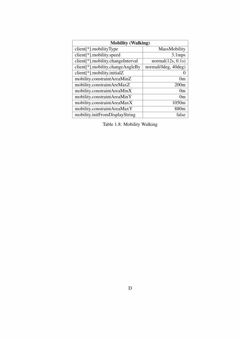
Mobility (Walking)client[*].mobilityType MassMobilityclient[*].mobility.speed 3.1mpsclient[*].mobility.changeInterval normal(12s, 0.1s)client[*].mobility.changeAngleBy normal(0deg, 40deg)client[*].mobility.initialZ 0mobility.constraintAreaMinZ 0mmobility.constraintAreMaxZ 200mmobility.constraintAreaMinX 0mmobility.constraintAreaMinY 0mmobility.constraintAreaMaxX 1050mmobility.constraintAreaMaxY 880mmobility.initFromDisplayString false

Table 1.8: Mobility Walking

D

Mobility (Driving)client[0].mobilityType RectangleMobilityclient[1].mobilityType RectangleMobilityclient[2].mobilityType RectangleMobilityclient[3].mobilityType RectangleMobilityclient[4].mobilityType RectangleMobilityclient[0].mobility.startPos 0client[0].mobility.constraintAreaMaxX 950mclient[0].mobility.constraintAreaMaxY 200mclient[1].mobility.startPos 1client[1].mobility.constraintAreaMaxX 500mclient[1].mobility.constraintAreaMaxY 500mclient[2].mobility.constraintAreaMaxX 960mclient[2].mobility.constraintAreaMaxY 860mclient[3].mobility.startPos 3client[3].mobility.constraintAreaMaxX 960mclient[3].mobility.constraintAreaMaxY 700mclient[4].mobility.startPos 3client[4].mobility.constraintAreaMaxX 100mclient[4].mobility.constraintAreaMaxY 860mclient[0].mobility.speed uniform(18.64mps, 24.85mps)client[1].mobility.speed uniform(18.64mps, 24.85mps)client[2].mobility.speed uniform(18.64mps, 24.85mps)client[3].mobility.speed uniform(18.64mps, 24.85mps)client[4].mobility.speed uniform(18.64mps, 24.85mps)client[5].mobilityType MassMobilityclient[6].mobilityType MassMobilityclient[7].mobilityType MassMobilityclient[8].mobilityType MassMobilityclient[9].mobilityType MassMobilitymobility.speed 9.6mpsmobility.changeInterval normal(12s, 0.1s)mobility.changeAngleBy normal(0deg, 45deg)client[10].mobilityType TractorMobilityclient[10].mobility.x1 5mclient[10].mobility.y1 5mclient[10].mobility.x2 960mclient[10].mobility.y2 860mclient[11].mobilityType TractorMobilityclient[11].mobility.x1 250mclient[11].mobility.y1 5mclient[11].mobility.x2 960mclient[11].mobility.y2 860m

E

client[12].mobilityType TractorMobilityclient[12].mobility.x1 500mclient[12].mobility.y1 300mclient[12].mobility.x2 960mclient[12].mobility.y2 860mclient[13].mobilityType TractorMobilityclient[13].mobility.x1 200mclient[13].mobility.y1 250mclient[13].mobility.x2 960mclient[13].mobility.y2 860mclient[14].mobilityType TractorMobilityclient[14].mobility.x1 5mclient[14].mobility.y1 400mclient[14].mobility.x2 960mclient[14].mobility.y2 860mmobility.speed 24.85mpsmobility.rowCount 4mobility.initialZ 0mobility.updateInterval 1smobility.constraintAreaMinZ 0mmobility.constraintAreaMaxZ 200mmobility.constraintAreaMinX 0mmobility.constraintAreaMinY 0mmobility.constraintAreaMaxX 960mmobility.constraintAreaMaxY 860m

Table 1.9: Mobility Driving

F

B Appendix 2 - Creating a new project

To create a new simulation project it requires a number of steps:

1. Start OMNeT++ IDE by double clicking on its icon, if using Windows,otherwise run omnetpp at a linux terminal.

2. Select a workspace to host your project. As a rule of thumb try to avoiddirectories with spaces.

3. From the File menu select New -> OMNeT++ project. Choose a nameand click next.

4. On this screen, choose Empty Project and click Finish or in case moreoptions are required choose "Next".

5. A default Network Description File (NED) should have been createdautomatically for you.

6. Should you desire to create a new NED file, choose File -> New ->Network Description File then select the project folder, choose a filename along with the “.ned” extension, select an Empty NED File andclick Finish. By default the new NED file will open in the design modewhere dragging and dropping components is possible. Of course, thereis the option to switch to source code mode, by clicking “Source” atthe bottom of the pane. With source mode one can copy-paste codefrom existing projects or write his/her own code.

7. The last component that is needed is the omnetpp.ini, which is theheart of any simulation as it contains all the parameters and configura-tions for all the scenarios. To create the file (if not there), navigate toFile -> New -> Initialisation File (ini) and choose the Empty Ini tem-plate. In case you are being asked to choose a network click Browse. . .and OMNeT will detect and propose the network in the NED file youcreated earlier. When done click Finish to conclude this step.

8. One last step that might be required if you choose to use the INETframework is: right click on your project and select Properties. At theleft pane there would be an option named "Project References" selectit, and on the right pane, locate and choose "inet".

Now the workspace and the project are ready for deployment. It is onlyneeded to define a network by adding the necessary components in the NEDfile, and set the right parameters in the omnetpp.ini file.

G

thesis project performance evaluation of routing protocols...

Documents