thesis mujgan omary

Biomass Energy Production Potential and Supply from Afforestation of

Wasteland in Rajasthan India

Mujgan Omary Studentnr:

Utrecht University Department of Science, Technology and Society Master program: Energy Science First supervisor (NL): Mr. B. Batidzirai MSc Second supervisor (NL): Prof. Dr. A.P.C. Faaij

Supervisor (India): Prof. Dr V. V. N. Kishore

1

Contents

1 INTRODUCTION ...................................................................................................................................................... 4

1.1 PROBLEM DEFINITION AND RESEARCH OBJECTIVES .............................................................................................. 5 1.1.1 Research question ........................................................................................................................................... 6 1.1.2 Scope and limitation ....................................................................................................................................... 6

2 WASTELANDS IN INDIA........................................................................................................................................ 7

2.1 WASTELAND CATEGORIES .................................................................................................................................... 8 2.1.1 Wasteland categorization by Directorate of Economics and Statistics........................................................... 8 2.1.2 Wasteland categorization by NRSA ................................................................................................................ 9

2.2 AVAILABILITY OF WASTELANDS IN INDIA AND THEIR SUITABILITY FOR PLANTATION ........................................ 10 2.2.1 Scrubland ...................................................................................................................................................... 13 2.2.2 Degraded forest ............................................................................................................................................ 13 2.2.3 Sand dunes and sands-desertic ..................................................................................................................... 13

2.3 REHABILITATION OF WASTELANDS .................................................................................................................... 13 2.4 DISCUSSION ....................................................................................................................................................... 15 2.5 SUMMARY .......................................................................................................................................................... 16

3 AFFORESTATION ................................................................................................................................................. 17

3.1 AFFORESTATION PROGRAMMES ......................................................................................................................... 18 3.1.1 Progress and achievements of afforestation programmes in India ............................................................... 19

3.2 FEASIBILITY OF AFFORESTATION ........................................................................................................................ 21 3.3 SMALL SCALE AFFORESTATION PROJECTS .......................................................................................................... 23 3.4 WASTELAND RECLAMATION AND BIOENERGY IN RAJASTHAN............................................................................ 25 3.5 DISCUSSION ....................................................................................................................................................... 26 3.6 SUMMARY .......................................................................................................................................................... 27

4 BIOMASS-BASED POWER................................................................................................................................... 29

4.1 BIOMASS POTENTIAL FROM WASTELANDS .......................................................................................................... 30 4.2 PROSOPIS JULIFLORA .......................................................................................................................................... 31 4.3 SUMMARY .......................................................................................................................................................... 33

5 METHODOLOGY................................................................................................................................................... 34

5.1 STATE AND WASTELAND SELECTION .................................................................................................................. 34 5.1.1 Study area ..................................................................................................................................................... 37

5.2 YIELD ESTIMATION ............................................................................................................................................ 37 5.2.1 Soil ................................................................................................................................................................ 38 5.2.2 Slope ............................................................................................................................................................. 42 5.2.3 Climate .......................................................................................................................................................... 44

5.3 SOIL AND TERRAIN, AND CLIMATE INDEX ........................................................................................................... 44 5.4 ECONOMIC PERFORMANCE ................................................................................................................................. 46 5.5 SUPPLY CHAINS PERFORMANCE.......................................................................................................................... 47 5.6 SENSITIVITY ANALYSIS ...................................................................................................................................... 49 5.7 LIMITATION IN METHODOLOGY AND DATA......................................................................................................... 49

6 DATA INPUT ........................................................................................................................................................... 50

6.1 STATE AND WASTELAND SELECTION: RAJASTHAN ............................................................................................. 50 6.1.1 Soil rating ..................................................................................................................................................... 55 6.1.2 Climate rating ............................................................................................................................................... 59 6.1.3 Climate rating and yield calculation............................................................................................................. 59

6.2 ECONOMIC PERFORMANCE ................................................................................................................................. 60 6.3 SUPPLY CHAINS PERFORMANCE.......................................................................................................................... 62 6.4 FREIGHT TRANSPORT AND ROAD CONNECTIVITY ................................................................................................ 64

6.4.1 Road connectivity and road density of Rajasthan ......................................................................................... 64

7 RESULTS AND DISCUSSION............................................................................................................................... 66

7.1 BIOMASS POTENTIAL .......................................................................................................................................... 66

2

7.2 COST OF BIOMASS PRODUCTION DISTRICT-WISE ................................................................................................. 71 7.3 TRANSPORTATION COST OF SELECTED BIOMASS SUPPLY CHAINS ....................................................................... 73

7.3.1 Biomass supply to thermal power plants (Co-firing) .................................................................................... 74 7.3.2 Supply of biomass to biomass-based power plants ....................................................................................... 80 7.3.3 Large scale biomass power plant.................................................................................................................. 84

7.4 COMPARISON BETWEEN COSTS OF ELECTRICITY PRODUCTION ........................................................................... 85 7.5 SENSITIVITY ANALYSIS ...................................................................................................................................... 88 7.6 DISCUSSION ....................................................................................................................................................... 91

7.6.1 Methodology ................................................................................................................................................. 91 7.6.2 Data .............................................................................................................................................................. 92 7.6.3 Comparison with other studies ..................................................................................................................... 93 7.6.4 Achievability of large scale plantation ......................................................................................................... 93

8 CONCLUSION AND RECOMMENDATION...................................................................................................... 95

8.1 CONCLUSION ...................................................................................................................................................... 95 8.2 RECOMMENDATION ............................................................................................................................................ 97

9 REFERENCES ......................................................................................................................................................... 98

10 APPENDICES ........................................................................................................................................................ 105

10.1 APPENDIX I WASTELAND RAJASTHAN ............................................................................................................. 105 10.2 APPENDIX II SOIL CHARACTERISTICS OF RAJASTHAN ...................................................................................... 106 10.3 APPENDIX III SOIL MAPPING UNIT OF RAJASTHAN DISTRICT-WISE ................................................................... 114 10.4 APPENDIX IV SLOPE......................................................................................................................................... 115 10.5 APPENDIX V CLIMATE CHARACTERISTICS........................................................................................................ 116 10.6 APPENDIX VI DISTRICT-WISE PRE-MONSOON GROUNDWATER LEVEL MAPS ..................................................... 118 10.7 APPENDIX VII NURSERY RAISING COSTS.......................................................................................................... 131 10.8 APPENDIX VIII COST CALCULATION OF BIOMASS CHIPPING CO-FIRING ............................................................ 132 10.9 APPENDIX IX COST CALCULATION OF BIOMASS DRYING (CO-FIRING) .............................................................. 133 10.10 APPENDIX X COST CALCULATION OF BIOMASS SIZING (CO-FIRING) ............................................................. 134 10.11 APPENDIX XI COST CALCULATION OF BIOMASS PELLETIZING (CO-FIRING) .................................................. 135 10.12 APPENDIX XII COST CALCULATION OF CHIPPING FOR SMALL SCALE BIOMASS POWER PLANTS .................... 136 10.13 APPENDIX XIII COST CALCULATION OF DRYING FOR SMALL SCALE BIOMASS POWER PLANTS ..................... 137 10.14 APPENDIX XII COST CALCULATION OF SIZING FOR SMALL SCALE BIOMASS POWER PLANTS ........................ 138 10.15 APPENDIX XII COST CALCULATION OF PELLETIZING FOR SMALL SCALE BIOMASS POWER PLANTS .............. 139 10.16 APPENDIX XVI DISTANCE BETWEEN DISTRICT HEADQUARTERS .................................................................. 140 10.17 APPENDIX XIII STATE-WISE ROAD LENGTH AND ROAD DENSITY ................................................................. 141 10.18 APPENDIX XIV VILLAGE CONNECTIVITY..................................................................................................... 142 10.19 APPENDIX XIX PRICE OF NON-COKING COAL ............................................................................................. 143 10.20 APPENDIX XX RAILWAY FREIGHT RATE AND GOODS CLASSIFICATION ........................................................ 144 10.21 APPENDIX XXI ESTIMATED COST OF SELECTED SUPPLY CHAINS BIOMASS POWER PLANTS FROM DISTRICTS

WITH THE LOWEST COST OF SUPPLY .............................................................................................................................. 145 10.22 APPENDIX VXII DISTRICT-WISE ESTIMATED COST OF SELECTED SUPPLY CHAINS BIOMASS BASED POWER

PLANTS 147 10.23 APPENDIX XXIII COST OF ELECTRICITY PRODUCTION BIOMASS BASED POWER PLANTS .............................. 151 10.24 APPENDIX XXIV SENSITIVITY ANALYSIS DISCOUNT RATE, LABOUR WAGES AND YIELD ............................. 153

3

List of Figures

FIGURE 1 SHARE OF HARD COAL TRADE ................................................................................................................................ 5

FIGURE 2 CUMULATIVE AFFORESTED AREA ......................................................................................................................... 19

FIGURE 3 AVERAGE SURVIVAL PERCENTAGE IN THE SAMPLED PLANTATIONS FOR DIFFERENT BIO-GEOGRAPHICAL ZONE ... 21

FIGURE 4 YEAR-WISE SURVIVAL UNDER VARIOUS MODELS ................................................................................................. 22

FIGURE 5 BIOMASS-BASED INSTALLED CAPACITY ACROSS SOME STATES OF INDIA TILL 2009 (MW) .................................. 29

FIGURE 6 YEAR WISE CAPACITY INCREASE IN BIOMASS BASED POWER ............................................................................... 29

FIGURE 7 CRITERIA FOR THE STATE CHOICE ......................................................................................................................... 36

FIGURE 8 STATE SELECTION ................................................................................................................................................ 36

FIGURE 9 SOIL MAP OF RAJASTHAN DISTRICT-WISE ............................................................................................................. 38

FIGURE 10 SOIL RATING ...................................................................................................................................................... 39

FIGURE 11 SOIL RATING OF LAND WITH SCRUB AND DEGRADED FORESTS ........................................................................... 39

FIGURE 12 SOIL RATING BIKANER DISTRICT ........................................................................................................................ 40

FIGURE 13 SOIL’S TEXTURAL CLASSES ................................................................................................................................ 41

FIGURE 14 YIELD ESTIMATION SAND-DUNES ....................................................................................................................... 41

FIGURE 15 SLOPE MAP OF RAJASTHAN ................................................................................................................................ 42

FIGURE 16 SLOPE RATING STEPS .......................................................................................................................................... 43

FIGURE 17 SLOPE AND WASTELAND MAP OF BIKANER ........................................................................................................ 43

FIGURE 18 PRE-MONSOON GROUNDWATER LEVEL MAP ....................................................................................................... 45

FIGURE 19 BIOMASS SUPPLY CHAIN..................................................................................................................................... 48

FIGURE 20 DISTRICT MAP OF RAJASTHAN ........................................................................................................................... 50

FIGURE 21: ANNUAL RAINFALL RAJASTHAN ....................................................................................................................... 51

FIGURE 22 DISTRICT-WISE WASTELAND AREA AND PERCENTAGE OF TOTAL GEOGRAPHICAL AREA ..................................... 51

FIGURE 23: WASTELAND MAP OF RAJASTHAN ..................................................................................................................... 52

FIGURE 24 SPATIAL ANALYSIS OF A SELECTED WASTELAND AREA IN DHOLPUR RAJASTHAN .............................................. 53

FIGURE 25 SPATIAL ANALYSIS OF A SELECTED WASTELAND AREA IN JAISALMER RAJASTHAN............................................ 54

FIGURE 26 BIOMASS POTENTIAL AND COST OF PRODUCTION ............................................................................................... 71

FIGURE 27 SUPPLY OF BIOMASS FROM JHALAWAR .............................................................................................................. 74

FIGURE 28 SUPPLY OF BIOMASS FROM KOTA ....................................................................................................................... 75

FIGURE 29 COST OF ELECTRICITY PRODUCTION CHHABRA THERMAL POWER PLANT ........................................................... 75


4

FIGURE 31 SUPPLY OF BIOMASS FROM BHILWARA .............................................................................................................. 76

FIGURE 32 COST OF ELECTRICITY PRODUCTION FOR KOTA THERMAL POWER PLANT .......................................................... 77


FIGURE 34 SUPPLY OF BIOMASS FROM JHALAWAR .............................................................................................................. 77


FIGURE 36 COST OF ELECTRICITY PRODUCTION KALISINDH THERMAL POWER PLANT ......................................................... 78

FIGURE 37 SUPPLY OF BIOMASS FROM AJMER ..................................................................................................................... 79


FIGURE 39 COST OF ELECTRICITY PRODUCTION SURATGARH THERMAL POWER PLANT ....................................................... 79

FIGURE 40 COST OF SELECTED SUPPLY CHAINS FROM KOTA (BARAN) ................................................................................ 80

FIGURE 41 COST OF ELECTRICITY PRODUCTION POWER PLANT BARAN ............................................................................... 81

FIGURE 42 COST OF SELECTED SUPPLY CHAINS FROM ALWAR (GANGANAGAR) .................................................................. 81

FIGURE 43 COST OF ELECTRICITY PRODUCTION POWER PLANT GANGANAGAR .................................................................... 81

FIGURE 44 COST OF SELECTED SUPPLY CHAINS (SIROHI) .................................................................................................... 82

FIGURE 45 COST OF ELECTRICITY PRODUCTION SIROHI POWER PLANT ................................................................................ 82

FIGURE 56 WASTELAND IN DISTRICTS WITH HIGHEST BIOMASS YIELD PER HECTARE .......................................................... 84

FIGURE 57 SUPPLY OF LOGS TO AJMER ................................................................................................................................ 84

FIGURE 58 COST OF ELECTRICITY PRODUCTION BIOMASS BASED POWER PLANT .................................................................. 85

FIGURE 49 COST OF POWER PRODUCTION FROM LOGS ......................................................................................................... 86

FIGURE 50 COST OF POWER PRODUCTION FROM PELLETS .................................................................................................... 86

FIGURE 51 SENSITIVITY ANALYSIS DISCOUNT RATE, LABOUR WAGES AND YIELD................................................................ 88

5

List of Tables

TABLE 1 WASTELAND CLASSIFICATION BY DIRECTORATE OF ECONOMICS AND STATISTICS ................................................. 9

TABLE 2 WASTELAND CATEGORIES ..................................................................................................................................... 10

TABLE 3 ESTIMATION OF WASTELANDS BY DIFFERENT AGENCIES ....................................................................................... 10

TABLE 4 WASTELAND AREA CATEGORY WISE (MHA) .......................................................................................................... 11

TABLE 5 STATE WISE WASTELAND COVER .......................................................................................................................... 12

TABLE 6 WASTELAND DEVELOPMENT PROGRAMMES .......................................................................................................... 13

TABLE 7 THE GREEN INDIA MISSION TARGETS.................................................................................................................... 18

TABLE 8 PROGRESS OF AFFORESTATION .............................................................................................................................. 19

TABLE 9 PLANTED AREA (2006-2010) ................................................................................................................................. 20

TABLE 10 PHYSICAL PROGRESS OF THE PLANTATION TILL 2007 .......................................................................................... 24

TABLE 11 ARAVALLI AFFORESTATION PROJECT ................................................................................................................. 25

TABLE 12 BIOMASS POWER GENERATION INSTALLED CAPACITY AND POTENTIAL ............................................................... 29

TABLE 13 STATE-WISE BIOMASS POTENTIAL FROM WASTELANDS ...................................................................................... 30

TABLE 14 CAPITAL COST AND LOAD FACTOR ...................................................................................................................... 31

TABLE 15 TREE SPECIES FOR DIFFERENT RAINFALL REGIONS .............................................................................................. 31

TABLE 16 REPORTED YIELD OF PROSOPIS JULIFLORA IN LITERATURE.................................................................................. 32

TABLE 17 YIELD PROSOPIS JULIFLORA IN SAND DUNES OF RAJASTHAN ............................................................................... 32

TABLE 18 SUITABILITY OF DIFFERENT WASTELAND CATEGORIES FOR PLANTATION ............................................................ 34

TABLE 19 SUITABILITY OF DIFFERENT WASTELAND CATEGORIES FOR PLANTATION ............................................................ 35

TABLE 20 WASTELAND CATEGORIES ACCORDING WAI 2011 .............................................................................................. 36

TABLE 21 USED SOURCES AND PROGRAMMES ..................................................................................................................... 37

TABLE 22 LAND-USE STATISTICS RAJASTHAN ..................................................................................................................... 50

TABLE 23 SOIL AND TERRAIN REQUIREMENTS USED FOR ESTIMATION OF YIELD FROM WL FOR PROSOPIS JULIFLORA......... 55

TABLE 24 SOIL BIKANER (SOIL MAPPING UNIT 3541) .......................................................................................................... 55

TABLE 25 RATING OF SOIL BIKANER (SOIL MAPPING UNIT 3541) ........................................................................................ 56

TABLE 26 SOIL BIKANER (SOIL MAPPING UNIT 3882) .......................................................................................................... 56

TABLE 27 RATING SOIL BIKANER (SOIL MAPPING UNIT 3882) ............................................................................................. 57

TABLE 28 AVERAGE RATING OF SOIL MAPPING UNITS ......................................................................................................... 57

TABLE 29 MECHANICAL COMPOSITION AND CHEMICAL CHARACTERISTICS OF DESERT SOIL ............................................... 57

TABLE 30 MECHANICAL COMPOSITION AND CHEMICAL CHARACTERISTICS OF SAND DUNES ................................................ 57

6

TABLE 31 SLOPE RATING ..................................................................................................................................................... 58

TABLE 32 SLOPE RATING BIKANER...................................................................................................................................... 58

TABLE 33 CLIMATE REQUIREMENTS PROSOPIS JULIFLORA .................................................................................................. 59

TABLE 34 OVEN DRY WEIGHT OF 6 YEARS OLD PROSOPIS JULIFLORA .................................................................................. 59

TABLE 35 RECOMMENDED PLANTATION DENSITIES FOR VARIOUS TYPES OF PROSOPIS JULIFLORA PLANTATION ................. 59

TABLE 36 DISCOUNT RATE .................................................................................................................................................. 60

TABLE 37 FOREST NURSERY ................................................................................................................................................ 60

TABLE 38 COST OF PLANTATION ......................................................................................................................................... 61

TABLE 39 LABOUR WAGES .................................................................................................................................................. 61

TABLE 40 DATA FOR ESTIMATING COST OF PRE-TREATMENT .............................................................................................. 62

TABLE 41 EXISTING POWER PLANTS IN RAJASTHAN ............................................................................................................ 62

TABLE 42 PROPERTIES OF PROSOPIS JULIFLORA IN DIFFERENT REGIONS.............................................................................. 63

TABLE 43 CONVERSION FACTORS ........................................................................................................................................ 63

TABLE 44 DENSITY OF PROSOPIS JULIFLORA ....................................................................................................................... 63

TABLE 45 ANNUAL OPERATING COSTS OF SMALL OPERATORS ESTIMATED BY WORLD BANK (RS) ..................................... 65

TABLE 46 DISTRICT-WISE AREA OF WASTELAND CATEGORIES 3, 4, 11 AND 17-19............................................................... 66

TABLE 47 DISTRICT-WISE SOIL MAPPING UNITS OF RAJASTHAN. ......................................................................................... 67

TABLE 48 SOIL AND TERRAIN, AND CLIMATE RATINGS FOR ESTIMATION OF AVERAGE YIELD PER HECTARE ....................... 67

TABLE 49 AVERAGE YIELD OF PROSOPIS JULIFLORA FROM WL CATEGORIES 3, 4 AND 11 (OVEN DRY)................................ 68

TABLE 50 YIELD OF PROSOPIS JULIFLORA PER SOIL MAPPING UNIT FOR 12 DISTRICTS WITH HIGHEST AVERAGE YIELD ...... 69

TABLE 51 BIOMASS YIELD FROM WL CATEGORIES 17-19 (OVEN DRY) ................................................................................ 70

TABLE 52 COST OF PRODUCTION FOR AVERAGE BIOMASS YIELD ......................................................................................... 71

TABLE 53 PRICE OF COAL $/GJ (HHV) ................................................................................................................................ 72

TABLE 54 AVERAGE FARMER SELLING PRICE OF MUSTARD HUSK ........................................................................................ 72

TABLE 55 COST OF TRANSPORTATION FOR SELECTED BIOMASS SUPPLY CHAINS ................................................................. 73

TABLE 56 COST OF SELECTED SUPPLY CHAINS FOR THERMAL POWER PLANTS ..................................................................... 74

TABLE 57 COST OF POWER PRODUCTION CO-FIRING ............................................................................................................ 74

TABLE 58 COST OF LOGS SUPPLY AND PRICE OF MUSTARD HUSK......................................................................................... 83

TABLE 59 COST OF ELECTRICITY PRODUCTION BIOMASS BASED POWER PLANTS ................................................................. 83

TABLE 60 HIGHEST AND LOWEST ESTIMATED YIELD OF PROSOPIS JULIFLORA VERSUS AVERAGE YIELD (TONNE/HA/YEAR) 88

TABLE 61 DISTRICT-WISE PRODUCTION POTENTIAL FROM 30 OF WL AREA (MILLION OVEN DRY TONNE PER YEAR) ........... 89

TABLE 62 YIELD OF PROSOPIS JULIFLORA BY VARYING THE RATING THE MOST LIMITING FACTORS (TONNE/HA/YEAR) ...... 89

7

TABLE 63 PRODUCTION POTENTIAL UNDER DIFFERENT SCENARIOS ..................................................................................... 90

8

List of Appendices

Appendix I

TABLE I 1 DISTRICT AND CATEGORY WISE WASTELANDS OF RAJASTHAN.......................................................................... 105

TABLE I 2 DISTRICT AND CATEGORY WISE WASTELANDS OF RAJASTHAN.......................................................................... 105

TABLE I 3 WASTELAND AREA WASTELAND ALLOTMENT (HA) ........................................................................................... 106

Appendix II

TABLE II 1 SOIL MAPPING UNIT 3541 ................................................................................................................................. 106

TABLE II 2 SOIL MAPPING UNIT3606.................................................................................................................................. 107








TABLE II 10 SOIL MAPPING UNIT 3781 ............................................................................................................................... 109


TABLE II 12 SOIL MAPPIN G UNIT 3797 .............................................................................................................................. 110












9

Appendix III

TABLE III 1 SOIL MAPPING UNIT OF RAJASTHAN DISTRICT-WISE ....................................................................................... 114

Appendix IV

TABLE IV 1 SLOPE AND SLOPE RATING DISTRICT-WISE...................................................................................................... 115

TABLE IV 2 DISTRICT-WISE AGRO-CLIMATIC ZONE. GROUNDWATER LEVEL AND CONSTRAINS FOR PLANTATION.............. 117

Appendix V

TABLE V 1 CLIMATE CHARACTERISTICS AND CLIMATE RATING ........................................................................................ 116

Appendix VI

TABLE VII 1 COST OF NURSERY RAISING .......................................................................................................................... 131

Appendix VII

TABLE VII 1 COST OF NURSERY RAISING .......................................................................................................................... 131

Appendix VIII

TABLE VIII 1 BIOMASS CHIPPING ...................................................................................................................................... 132

Appendix IX

TABLE IX 1 BIOMASS DRYING ........................................................................................................................................... 133

Appendix X

TABLE X 1 BIOMASS SIZING (HAMMER-MILL) ................................................................................................................... 134

Appendix XI

TABLE XI 1 PELLETIZING OF BIOMASS............................................................................................................................... 135

Appendix XII

TABLE XII 1 CHIPPING OF BIOMASS................................................................................................................................... 136

Appendix XIII

TABLE XIII 1 DRYING OF BIOMASS.................................................................................................................................... 137

Appendix XIV

TABLE XIV 1 SIZING OF BIOMASS ..................................................................................................................................... 138

Appendix XV

TABLE XV 1 PELLETIZING OF BIOMASS ............................................................................................................................. 139

Appendix XVI

TABLE XVI 1 2ND

TRANSPORTATION DISTANCE THERMAL POWER PLANTS ......................................................................... 140

10

TABLE XVI 2 2ND

TRANSPORTATION DISTANCE BIOMASS BASED POWER PLANTS ............................................................... 140

Appendix XVII

TABLE XVII 1 ROAD LENGTH AND ROAD DENSITY OF INDIA ............................................................................................. 141

Appendix XVIII

TABLE XVIII 1 DISTRICT-WISE VILLAGE CONNECTIVITY .................................................................................................. 142

Appendix XIX

TABLE XIX 1 PRICE OF COAL ............................................................................................................................................ 143

Appendix XX

TABLE XX 1 RAILWAY FREIGHT RATE PER TONNE ............................................................................................................ 144

TABLE XX 2 CLASSIFICATION OF GOODS .......................................................................................................................... 144

Appendix XXI

FIGURE XXI 1 COST OF SELECTED SUPPLY CHAINS FOR JAIPUR FROM AJMER ................................................................... 145

FIGURE XXI 2 COST OF SELECTED SUPPLY CHAINS JALORE FROM JALORE ........................................................................ 145

FIGURE XXI 3 COST OF SELECTED SUPPLY CHAINS KOTA FROM KOTA ............................................................................. 145

FIGURE XXI 4 COST OF SELECTED SUPPLY CHAINS FOR NAGAUR FROM ............................................................................ 146

FIGURE XXI 5 COST OF SELECTED SUPPLY CHAINS FOR TONK FROM TONK ...................................................................... 146

Appendix XXII

TABLE XXII 1 COST OF PRODUCTION AT THE POWER PLANT GATE BARAN DISTRICT ($/GJ) ............................................. 147

TABLE XXII 2 COST OF PRODUCTION AT THE POWER PLANT GATE GANGANAGAR DISTRICT ($/GJ).................................. 147

TABLE XXII 3 COST OF PRODUCTION AT THE POWER PLANT GATE JAIPUR DISTRICT ($/GJ) .............................................. 148

TABLE XXII 4 COST OF PRODUCTION AT THE POWER PLANT GATE JALORE DISTRICT ($/GJ) ............................................. 148

TABLE XXII 5 COST OF PRODUCTION AT THE POWER PLANT GATE KOTA DISTRICT ($/GJ)................................................ 149

TABLE XXII 6 COST OF PRODUCTION AT THE POWER PLANT GATE NAGAUR DISTRICT ($/GJ) ........................................... 149

TABLE XXII 7 COST OF PRODUCTION AT THE POWER PLANT GATE SIROHI DISTRICT ......................................................... 150

TABLE XXII 8 COST OF PRODUCTION AT THE POWER PLANT GATE TONK DISTRICT ($/GJ) ................................................ 150

11

Appendix XXIII

FIGURE XXIII 6 BIOMASS POWER PLANT JAIPUR ............................................................................................................... 151

FIGURE XXIII 7 BIOMASS POWER PLANT JALORE .............................................................................................................. 151

FIGURE XXIII 8 BIOMASS POWER PLANT KOTA ................................................................................................................ 151

FIGURE XXIII 9 BIOMASS POWER PLANT NAGAUR ............................................................................................................ 152

FIGURE XXIII 10 BIOMASS POWER PLANT TONK............................................................................................................... 152

Appendix XXIV

FIGURE XXIV 1 SENSITIVITY ANALYSIS DISCOUNT RATE .................................................................................................. 153




FIGURE XXIV 5 SENSITIVITY ANALYSIS LABOUR WAGES .................................................................................................. 154




FIGURE XXIV 9 SENSITIVITY ANALYSIS YIELD ................................................................................................................. 155

List of abbreviations

BRAI Biomass Resource Atlas of India

DOLR Department Of Land Resources

CGP Central Gathering Point

CGWB Central Ground Water Board

GOI Government of India

HWSD Harmonized World Soil Database

COP Cost of Production

Gov of Raj Government of Rajasthan

IIED International Institute for Environment and Development

JFM Joint Forest Management

kt Kilo tonne

MNRE Ministry of New and Renewable Energy

MOEF Ministry of Environment and Forests

MOA Ministry of Agriculture

MORD Ministry of Rural Development

mha million hectare

mt Million tonne

NAEB National Afforestation and Eco-development Board

NAP National Afforestation Programme

NBSS&LUP National Bureau of Soil Survey and Land Use Planning

NFP National Forest Policy

NRSA National Remote Sensing Agency

NWDB National Wasteland Development Board

PC Planning Commission

RREC Rajasthan Renewable Energy Corporation Limited

SPWD Society for Promotion of Wasteland Development

TGA Total Geographical Area

Wl Wasteland

WAI Wasteland Atlas of India

Summary

Population growth, poverty and utilization of natural resources in India have increased the pressure on arable land and forests which led to land degradation. Degraded lands are called wastelands in India. The National Wasteland Development Board defines wasteland as degraded land which is currently underutilized, deteriorating due to lack of appropriate water and soil management or natural causes but it can be brought

under vegetative cover with reasonable efforts. Based on available reports, the area of wasteland ranged from 30 to 175 million hectares in India. The variation on the extent of wasteland was due to different definitions for different categories of wastelands, use of different databases and methodologies for obtaining information on wastelands by diverse agencies. National Remote Sensing Agency on behest of Ministry of Rural Development used three season satellite data to estimate the area of different wasteland categories for 2006. In 2008, the three seasons satellite data was harmonized by Indian Council of Agriculture Research and National Remote Sensing Agency and also a

practical and management-responsive estimation on wastelands was conducted. Wasteland is classified in 23 categories and the total estimated extent of wasteland was 47.2 million hectare, which is 15% of the total geographical area of India. The results of estimated area were published in Wasteland Atlas of India in 2010. After the publication of 2010, the change in area of different wasteland categories between 2006 and 2009 was again estimated and the results were published in Wasteland Atlas of India 2011. The most recent estimation of wasteland area is around 46.7 million hectare. The area of wasteland for all the states is presented by

category and district. The largest wasteland categories are land with dense-scrub, land with open-scrub and under-utilized /degraded forest-scrub which cover 57% of total wasteland area. The largest area for the first two categories can be found in the states of Rajasthan, Maharashtra, Madhya Pradesh, Gujarat and Andhra Pradesh. The wasteland category underutilized/degraded forest scrub-dominated is mostly located in the states of Andhra Pradesh, Madhya Pradesh, Rajasthan and Maharashtra. The states of Rajasthan, Jammu &Kashmir and Madhya Pradesh have the largest area of wasteland with 18%, 16% and 9% respectively.

Deforestation and land degradation were the triggers for the government, private sector and foreign agencies to come up with numerous attempts to stop deforestation, stimulate afforestation and rehabilitate wastelands. The National Forest Policy in 1894 was the first move of the government to tackle forest degradation by stressing on conservation of forests in order to maintain environmental stability and meet the basic needs of communities living at the forest fringes. The National Forest Policy was the forerunner of the green movement in India. In 1952, the policy was revised and it emphasized on increasing the tree cover behind the established forests. One of the objectives was to bring 33% of the total geographical area under tree cover by 2012.

Afforestation started in the late 1950s and plantation activities were carried out under different programmes. The main objectives of these programmes were conserving the environment and meeting the wood demand by planting fast growing species suitable for fuel-wood and timber. Externally aided social forestry projects were also implemented during 1980-1992 with the same objectives by targeting degraded forests. Community-land plantations have also been launched on wastelands owned by the government and private. All the efforts resulted in afforestation of almost 35 million hectare land from 1950 to 2005. In addition an area of 7.3 million hectare was planted since the establishment of Twenty Point Programme in 2006. The average annual

plantation rate between 1980 and 2005 was 1.32 million hectare and the target annual plantation rate for 2010-2011 was 1.8 million hectare per year. The annual plantation rate was and still is below the required plantation rate to bring one third of the country under forest cover. The government also launched many programmes like National Watershed Development Project for Rainfed Areas, Watershed Development in Shifting Cultivation Areas, Drought Prone Areas Programme, Desert Development Programme, Integrated Wasteland Development Programme, and Employment Assurance Schemes to rehabilitate wastelands. Other aims of these programmes are to increase tree cover, meet the

growing wood and energy demand and to create rural employment. In 2009 the National Policy on bio-fuels adopted a non-mandatory 20% blending of bio-diesel and bio-ethanol by 2017 and the plantation for biofuels would only take place on wastelands.

1

The ministry of Environment and Forest brought four schemes with similar goals under National Afforestation

Programmes in order to prevent overlap between different schemes and create transparency. However, there still exist other schemes with similar goals e.g. afforestation project under wasteland development programmes. As part of rural and wasteland development programmes, large-scale plantations and social forestry projects were launched in several states in the early 1980s. Because the supply of wood from government-owned forests has been declining it is believed that afforestation of wasteland is emerging as a big enterprise in India to meet the demand of wood-based industries. Consistent with a study on economic performance of afforestation, afforestation of wastelands is financially feasible, even without taking non-

market benefits into account. However, the rate of return on the investments made on afforestation by Indian government over the past decades was low. The reasons for low return were utilization of poor technology, low quality seed, low yield and lack of maintenance. Even if afforestation is economically feasible, substantial investments are needed for large-scale afforestation of wastelands. Biomass provides about one third of India’s total primary energy supply. According to estimations of Ministry of New and Renewable Energy around 540 million tonnes of biomass are available in India annually. This

includes residues from agriculture, agro-industry, forestry, and plantations. Biomass Resource Atlas of India project was carried out to assess the biomass availability excluding the current usage. The atlas contains data on agro-residues, biomass potential from forests and wastelands as extension of forests. The total estimated biomass potential from wastelands is around 6.2GWe while the installed biomass-based capacity was 2.6GWe at the end of 2010. The states of Uttar Pradesh and Andhra Pradesh have the highest installed capacities whereas Punjab and Rajasthan have the lowest installed capacities. According to Ministry of New and Renewable energy, biomass-based power plants use agro-residues and woody biomass from dedicated energy plantations.

The main objective of this paper was to estimate the potential of biomass from most suitable wasteland categories in the state of Rajasthan and to assess economic performance of biomass supply chains. The yield per hectare was estimated for Prosopis juliflora tree because it can be planted on low nutrient and quality soils. This tree species can survive in low rainfall region, provides high quality fuel-wood and has been used for reclamation of degraded land in the arid and semi-arid parts of India. The reported yield of this plant is between 11-20t/ha/year in India. Nevertheless low yield of 0.6-1.8t/ha/year has also been reported in low

rainfall regions. The estimated biomass potential from plantation of wasteland categories land with open scrub, land with dense scrub and degraded forests is around 19.3 million tonne per year based on the obtained results in this study. The biomass potential from 30% of mentioned wasteland categories, as it was assumed that only 30% of wasteland would be available for plantation, is around 5.8 million tonne per year. And the cost of production ranges between 2 to 13.3 $/GJ. The cost of production is lowest in district of Ajmer and highest in

district of Jaisalmer. The potential from wasteland categories sand-dunes and sands-desertic is around 1.2 million tonne per year. If 30% of these categories would be used for plantation, it can deliver 0.4 million tonne per year. The districts of Ajmer and Sirohi have the highest yield from these categories with 1.8 tonnes per hectare per year. The lowest yield is obtained from Barmer, Bikaner and Jaisalmer which is less than 2 tonnes per hectare in six years. The yields from these categories are too low to be used for energy plantation as the cost of production of biomass would be very high.

The estimated cost of transportation in India is around $0.05t-1km-1 and the calculated cost of transportation from CGP to the thermal power plants ranges between $0.5-4.5 /GJ, $0.5-5/GJ for chips and $0.4-3.5/GJ for pellets. The cost of transportation for pellets is lower than for logs, however due to low transportation cost in India the difference is very small to have an impact on the cost of supplied biomass. Pre-treatment of biomass for the purpose of decreasing transportation cost can only have opposing impact on the cost of biomass at the power plant gate since cost of pre-treatment is much higher than the difference between costs of

transportation. In supply of biomass the cost of transportation plays less important role in India because of low transportation cost. Nevertheless, connectivity of the villages by road plays a more important factor in supply of biomass, because limited number of villages in Rajasthan with low population is connected by road.

2

The supply of biomass logs (production plus transportation) for coal-based power plants, under the study costs

3.4-6.1$/GJ, if it is supplied from Ajmer, Bhilwara, Jhalawar and Kota districts. The supply of biomass from these districts is the most economic option compared to other districts. The price of different coal grades ranges between 0.8-3.2 $/GJ without transportation costs. Most of the coal based power plants in India use low grade coal. The price of low grade coal is around 0.8$/GJ which is much more economical than the usage of biomass. The cost of supplied logs to eight small scale biomass-based power plants also under the study in Rajasthan is

3.1-6.5$/GJ; if it is delivered from Ajmer, Alwar, Kota, Jalore, Sirohi and Tonk, while the price of mustard husk used by these power plants ranged between 2.1-4.4$/GJ. Supply of biomass from other districts is comparatively higher than the mentioned districts. Based on the yield estimations and considering the relevant factors e.g. availability of wasteland and road connectivity the best location to setup a large scale biomass-based power plant is between districts of Ajmer, Bhilwara, Pali and Rajsamand. The cost of power production is lowest for co-firing and ranges 58-82$/MWhe for logs, 59-85$/MWhe for

chips and 62-81$/MWhe for pellets. For the thermal power plant located in Ganganagar, cost of power production is the lowest if biomass supplied as pellets. The cost of electricity production for large scale power plant is $86/MWhe for logs, $88/MWhe for chips and 91 $/MWhe for large scale biomass-based power plant. The cost of power production for small scale biomass power plants in Rajasthan is between 149 and 233$/MWhe. For all the existing biomass based power plants in Rajasthan, supply of biomass and cost of power production is the lowest if biomass is supplied as logs, except for the power plant located in Ganganagar. The supply of logs at the power plant gate is the lowest for logs, however when looking at the cost of power production, supply of pellets are more economical than logs.

The best option to increase the share of biomass-based power would be biomass co-firing. Not only the cost of power production is low for biomass co-firing, the power plant can also keep operating if biomass would not be available. Another advantage of co-firing is that up to 444MW biomass power capacity could be generated by four coal-based power plants in Rajasthan by replacing up to 10% of their annual coal usage.

3

Preface

The topic of this research was chosen out of curiosity for energy plantation on degraded lands, and passion and love for India and developing countries. This study wouldn’t have been possible without hard work, interest in the topic and support of several people. This is a good opportunity for me to express my sincere gratitude to:

André Faaij: thank you for making it possible for me to conduct this research and being the first one providing me with details on the topic of my thesis Bothwell Batidzirai: thank you for all your patience, intensive feedback, active involvement and moral support Birka Wicka: thank you for providing me the method you used in your own research and your time

explaining it, without your method I wouldn’t have been able to develop a method in this research Judith Verstegen: thank you for your effort and patience explaining me how to use the slope function in Arcmap Jenske van Eijk: thank you for offering your help and providing me relevant papers

Dr.V.V.N. Kishore: thank you for making it possible to conduct interview at the Ministry of Environment and Forests, for your hospitality at your University and mental support during my stay in Delhi. Viren Lobo: thank you for giving your time and providing me information on wasteland, and explaining the concept and history of wasteland in India SN SriNivas: thank you for receiving me at UNDP and providing me information on Bioenergy for Rural

India project Last but not least, thanks to my dear family and friends (Mariësse van Sluisveld, Seema Gogia and Ranjana Sharma) for their support during my research.

4

1 Introduction

India is one of the emerging economies with a constant GDP growth exceeding 8% for the past years and the expectation is that this growth will continue. Such a high growth is essential for India to eliminate poverty and meet its economic and human developing goals. Energy is a key driver of this growth and its availability is essential to sustain this growth. Based on official projections of the Planning Commission (PC), the energy demand in India is expected to be three to four times of the current level in 25 years. Due to such an

extraordinary growth, India is expected to face challenges in meeting its energy demand (PC. 2005; Ravindranath& Balachandra. 2009). According to the World Energy Outlook (WEO) 2009, global energy demand is expected to increase by 1.5% per year between 2007 and 2030 and India alone will account for 15% of the global energy demand growth (IEA. 2009). To meet its energy demand, India is importing 30% of its energy needs. Along with the growing demand, the share of fossil fuel is increasing, which makes India more dependent on import from oil rich

regions (PC. 2005). Above all, it is projected by International Energy Agency (IEA), that India would be responsible for 2Gt energy-related CO2 emissions growth in 2030, which is 18% of the total global emissions growth (IEA. 2009). To reduce its fossil energy related GHG emissions, India needs to increase its share of renewable energy. Afforestation/reforestation1 of degrade lands with energy plantation could be a solution to growing energy demand and to increasing energy related CO2 emission. India has enormous areas of degraded land, which are defined as wastelands. These wastelands are the result of either intrinsic characteristic such as location,

environment, chemical, and physical properties of the soil or lack of proper management (Balooni& Singh. 2003; Ravindranath et al. 2008). The soil fertility of wastelands is low and there is no or little irrigation potential. Therefore, these wastelands are not suitable for food crops that require fertile soil and continuous water supply. Afforestation in India started in 1950, however, large-scale afforestation started in the 1980s. Afforestation/reforestation in India was carried out under different programmes such as social forestry

programme started in the early 1980s, Joint Forest Management Programme started in 1990, and afforestation under national Afforestation and Eco-development Board programmes started in 1992. One of the objectives of the above-mentioned programmes is to increase forest cover through afforestation on degraded and unproductive land to meet the demand of fuel-wood, fodder, and timber (Ravindranath et al. 2008). Besides meeting the fuel-wood demand, afforestation can also provide socio-economic and environmental benefits. The plantation activities create rural employment in establishing, protecting, and maintaining of

plantations. It also provides diverse biomass products like fodder, timber, non-timber forest products such as fruits, oil seeds, leaves, gum, honey, etc. The environmental benefits include conservation of biodiversity and watershed protection. In addition, forest carbon sinks would be conserved as biomass needs will be met from afforestation/reforestation activities (Ravindranath et al. 2001). Energy plantations (afforestation with dedicated energy crops) can help India to improve its energy security, as the capacity for such plantations is significant. If 10 million hectares of wasteland is converted to fuel-wood plantation with a sustained yield of 100 million tonnes of wood annually, 100 million tonnes of

domestic coal can be replaced since the calorific value of Indian coal is identical to wood. According to PC, if fuel-wood plantations are developed in India, biomass can be a major source of energy (PC. 2005). Moreover, if plantation of dedicated energy crops is economically feasible and environmentally sound, it will help India to reduce its share in energy related CO2 emission.

1 Afforestation is the establishment of a forest in an area where the preceding vegetation or land use was not a forest. Reforestation is the

reestablishment of forest cover after the previous forest was removed

5

1.1 Problem definition and research objectives

As India alone contributes to 15% of global energy-consumption growth and to 18% of energy related CO2

emission, it is necessary to assess the availability and contribution of biomass from wastelands to power

generation, as more than 67% of power in India was being generated from coal in 2009. According to projections by WEO 2010, India will surpass China as the biggest coal importer around 2020, see figure 1 (IEA. 2010; IEA. 2011).

Figure 1 Share of hard coal trade

Source: (IEA. 2010)

Biomass can be a major source of energy to meet this expected increase in energy demand yet continuous supply of biomass needs production of energy crops e.g. fuel-wood plantations to meet the demand. India has large areas of wasteland that can be used for production of biomass for power plants and for other commercial uses, especially for rural area without electricity access. At the same time utilization of wastelands for energy plantations, will help rehabilitate the degraded lands and prevents the overexploitation and destruction of forests.

The extent of wasteland has been determined by many organizations in the past giving different estimations, making an accurate estimation of biomass potential difficult. In addition, most studies until now focused partially on economic performance of afforestation/reforestation. Less attention has been paid to supply chain aspects of biomass energy from wastelands in India. Having insight on the logistics and supply strategies is the key to a competitive bio-energy industry in the country.

Land availability, biomass productivity, economic performance of plantation and logistic infrastructure are important factors in determining the economic potential of biomass in India. To assess the contribution of biomass from plantation of wastelands with energy crops, it is essential to collect data on wastelands and forestry activities intended to meet the biomass demand. The aim of this study was to assess the potential supply of biomass from wasteland in Rajasthan India. A method was developed to assess the potential of biomass from six wasteland categories. The economic performance of wasteland afforestation of three suitable wasteland categories and multiple supply chains for

four coal-based power plants, eight small scale biomass-based power plants and a large scale non-existing biomass-based power plant was estimated. The objectives of this study were to gather accurate and recent data on estimation of wasteland area in India, its suitability for energy plantation in order to identify major wasteland categories with best prospect for biomass production and afforestation/plantation activities in India (i.e. progress, scale and economic performance, suitable tree species). Subsequently, the technical potential of biomass obtained from plantation

of suitable wasteland categories; as well their economic performances were assessed. Lastly, the performance of biomass supply chains in the state of Rajasthan from feedstock production to the gate of existing power plants was assessed.

6

1.1.1 Research question

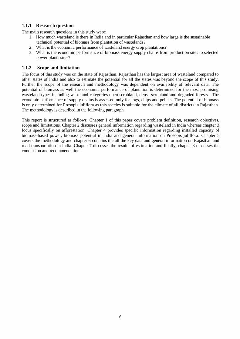
The main research questions in this study were: 1. How much wasteland is there in India and in particular Rajasthan and how large is the sustainable

technical potential of biomass from plantation of wastelands?

2. What is the economic performance of wasteland energy crop plantations? 3. What is the economic performance of biomass energy supply chains from production sites to selected

power plants sites?

1.1.2 Scope and limitation

The focus of this study was on the state of Rajasthan. Rajasthan has the largest area of wasteland compared to other states of India and also to estimate the potential for all the states was beyond the scope of this study. Further the scope of the research and methodology was dependent on availability of relevant data. The potential of biomass as well the economic performance of plantation is determined for the most promising

wasteland types including wasteland categories open scrubland, dense scrubland and degraded forests. The economic performance of supply chains is assessed only for logs, chips and pellets. The potential of biomass is only determined for Prosopis juliflora as this species is suitable for the climate of all districts in Rajasthan. The methodology is described in the following paragraph. This report is structured as follows: Chapter 1 of this paper covers problem definition, research objectives, scope and limitations. Chapter 2 discusses general information regarding wasteland in India whereas chapter 3 focus specifically on afforestation. Chapter 4 provides specific information regarding installed capacity of

biomass-based power, biomass potential in India and general information on Prosopis juliflora. Chapter 5 covers the methodology and chapter 6 contains the all the key data and general information on Rajasthan and road transportation in India. Chapter 7 discusses the results of estimation and finally, chapter 8 discusses the conclusion and recommendation.

7

2 Wastelands in India

Rapid industrialization, economic development and population growth have put an enormous pressure on land leading to degradation of it in all parts of India. To increase biomass production and to restore the environment, preventative and restorative measures are necessary for rehabilitation of degraded lands (MORD. 2010b). That is why, information on the nature, amount, and severity of degradation is necessary in attempt to reclaim these degraded lands and use them for plantation.

The degraded lands are called wastelands in India and the concept of wasteland was introduced during the

British rule of India and originated from the perspective of revenue rather than ecology (Bhumbla& Khare. 1984). Lands that were not under cultivation, hence non-revenue lands, were classified as wastelands and its proprietary rights were claimed by the state. In post-independence era, wastelands were viewed as empty land available for expanding agriculture and setting agricultural labourers. The focus of the government was more on expansion of agriculture in order to make the country more self-sufficient in food. However, this view changed when the country achieved self-sufficiency in food in the 1970s and the degradation of forests and shortages of fuel-wood and fodder were the main challenges. In the 1980s, a massive afforestation programme

was launched to bring 33% of the country under tree cover. Later, the emphasis shifted more towards addressing the challenges of global warming (Bhumbla& Khare. 1984; Saigal. 2011).

To rehabilitate the degraded lands, National Wasteland Development Board (NWDB) was setup under the Ministry of Environment and Forests by the Government of India in 1985 with the objective of reclaiming 5mha of degraded land each year for fuel-wood and fodder production through a massive programme of seeding and afforestation. Subsequently, a separate Department of Wasteland Development in the Ministry of Rural Development and Poverty Alleviation was created in 1992 and NWDB was transferred to this department. This department was later renamed as Department of Land Resources to act as nodal agency for

land resources management. This department is implementing three area Development Programmes on watershed basis namely, Integrated Wasteland Development Programme (IWDP), Drought Prone Areas Programme (DPAP) and Desert Development Programme (DDP) with aim to treat barren lands (MORD. 2010a; MOEF. 2006).

The definition of wasteland according to oxford dictionary2 is an area of land that cannot be used or that is no longer used for building or agriculture (OALD. 2011). The estimated productivity of wastelands compared to agricultural land is less than 20% of constraint free yields 3 (Garg et al. 2011). The soil organic carbon levels are severely reduced due to soil degradation process, which is primary caused, by low biomass productivity and removal of crop-residues in large amounts (Balooni& Singh. 2003; Ravindranath& Hall. 1995).

Society for Promotion of Wasteland Development (SPWD) indicates that there is no consensus on the definition for wastelands. An economic potential and actual returns based definition was accepted for a short time, which stated that any land that gives less than 20% of its economic potential is a wasteland. According to SPWD, this definition is not very practical for estimating the extent of wasteland because it is based on productivity, which depends on the state of the technology and its actual application. Together with improvement in technology, the productivity of land increases as well. However, the actual increase in production will depend on the acceptance and application of improved technology over a period of time. Therefore, this definition makes wastelands a function of state of technology, frequency of its acceptance and

time. A change in any of these factors shall change the description of a piece of land into wastelands. Based on this definition, any land with ecological hazard is not considered as wasteland if the land has proper economic returns (Bhumbla& Khare. 1984).

One of the objectives of SPWD is to develop a working definition for wastelands that helps to estimate the wasteland area and at the same time considers ecological concern as well. The definition used by SPWD for quantitative estimation of wasteland is: ―Those lands which are (a) ecologically unstable (b) whose top soil has been nearly completely lost and (c) which have developed toxicity in the root zones for growth of most plants,

2 Oxford Advanced Learner’s Dictionary 3 Maximum potential yield of a certain crop where factors such as soil suitability, moisture stress or workability parameter are not

taken into consideration(Stewart. 1981)

8

both annual crops and trees‖. This definition covers lands that are affected by water erosion, wind erosion,

floods, waterlogging, soil salinization and soil alkalinisation (Bhumbla& Khare. 1984). According to Ministry of Rural Development, Department of Land Resources, wastelands are not currently being used and if these wastelands cannot be reclaimed, they can be used for other commercial purposes (Chaudhary. 2011). In contrast to MORD DOLR, SPWD stated that the so-called wastelands are being used by villagers in various ways like grazing and marginal agriculture. Thus, the term wasteland is not a proper word to refer degraded lands with and this view was shared by MOEF as well (Saxena. 2011; Baka. 2011).

The Wasteland Atlas of India uses the definition of NWDB for wasteland which defines wasteland as: ―Wasteland is degraded land that can be brought under vegetative cover with reasonable

4 efforts and which

is currently under-utilized and or/land that is deteriorating due to lack of appropriate water and soil management or due to natural causes. Wasteland occurs from inherent/or imposed constraints such as location, environmental conditions, chemical and physical properties of the soil and/or financial and management constraints‖ (WAI, 2010). Barren rocky areas are example degraded land due to inherent/ or imposed constraints. In addition, social factors like population growth, poverty are the causes of land degradation. Explosive population growth has increased the pressure on arable land leading to an increase in utilization of natural resources (Ministry of Finance.; MOEF. 2001b).

According to SPWD, the definition of wasteland should include that some wasteland categories are currently

being used, but they can be used more productively. The definition of NWDB for wastelands does not define what reasonable effort entails, nonetheless reasonable effort can be defined as maximum total cost per hectare that does not exceed the released budget for a certain project per hectare for rehabilitation of wasteland. Despite disagreement on the definition of wasteland, all scientific reports and government organizations use the definition of NWDB for wastelands.

2.1 Wasteland categories

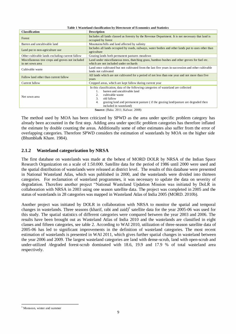
Wasteland categories have been identified by various government organizations and individuals (Baka. 2011; Kalwar. 2008). The main sources of wasteland categorizations/classification are the estimations conducted by National Remote Sensing Agency (NRSA) on behest DOLR MORD and the Directorate of Economics and Statistics (MORD. 2010b; Baka. 2011). The identification by these two main sources is given in the following sub-paragraphs.

2.1.1 Wasteland categorization by Directorate of Economics and Statistics

The Directorate of Economics and Statistics within the Ministry of Agriculture (MOA)

has classified wastelands into cultivable and uncultivable wastelands and this classification is usually referred as Nine-Fold classification. The land use is categorized into nine land use categories and land that has not been under cultivation for the past five years but was cultivated at some point in the past, have been brought under cultivable wasteland. Land that never has been cultivated like desserts and rocky-land are classified as uncultivable wastesland, see table 1 (Baka. 2011; Kalwar. 2008; Trivedi. 2010; Ramachandra& Kamakshi. 2005).

The assessments for wastelands are gathered annually with a two-year gap in the publication of the assessments. The statistics are based on village land settlement records maintained by the village administrative officer and the most recent statistics are from the year 2008. Every year in the month of May or June, settlements are conducted at village-wide meeting. The directorate of Economics and Statistics passes the settlement records along the district, state and central government levels and the records are merged together (Baka. 2011; Kalwar. 2008). The area of wastelands is determined by assuming a certain percentage of area under each category of land-use as problem area. Subsequently the problem area is estimated and

added to the assumed area in the first step.

4 What reasonable effort entails is not defined

9

Table 1 Wasteland classification by Directorate of Economics and Statistics

Classification Description

Forest Includes all lands classed as forestry by the Revenue Department. It is not necessary that land is

occupied by forest

Barren and uncultivable land Mountains/hills and land affected by salinity

Land put to non-agriculture use Includes all lands occupied by roads, railways, water bodies and other lands put to uses other than

agriculture

Other cultivable lands excluding current fallow Grazing lands both permanent pastures meadows

Miscellaneous tree crops and groves not included

in net sown area

Land under miscellaneous trees, thatching grass, bamboo bushes and other groves for fuel etc.

which are not included under orchards

Cultivable waste Land once cultivated but not cultivated from the last five years in succession and other cultivable

lands not cultivated

Fallow land other than current fallow All lands which are not cultivated for a period of not less than one year and not more than five

years

Current fallow Cropped areas, which are kept fallow during current year

Net sown area

In this classification, data of the following categories of wasteland are collected

1. barren and uncultivable land

2. cultivable waste

3. old fallow

4. grazing land and permanent pasture ( if the grazing land/pasture are degraded then

included in wasteland)

Source: (Baka. 2011; Kalwar. 2008)

The method used by MOA has been criticized by SPWD as the area under specific problem category has already been accounted in the first step. Adding area under specific problem categories has therefore inflated

the estimate by double counting the areas. Additionally some of other estimates also suffer from the error of overlapping categories. Therefore SPWD considers the estimation of wastelands by MOA on the higher side (Bhumbla& Khare. 1984).

2.1.2 Wasteland categorization by NRSA

The first database on wastelands was made at the behest of MORD DOLR by NRSA of the Indian Space Research Organization on a scale of 1:50.000. Satellite data for the period of 1986 until 2000 were used and

the spatial distribution of wastelands were released at district level. The results of this database were presented in National Wasteland Atlas, which was published in 2000, and the wastelands were divided into thirteen categories. For reclamation of wasteland programmes, it was necessary to update the data on severity of degradation. Therefore another project ―National Wasteland Updation Mission was initiated by DoLR in collaboration with NRSA in 2003 using one season satellite data. The project was completed in 2005 and the status of wastelands in 28 categories was mapped in Wasteland Atlas of India 2005 (MORD. 2010b).

Another project was initiated by DOLR in collaboration with NRSA to monitor the spatial and temporal changes in wastelands. Three seasons (kharif, rabi and zaid)5 satellite data for the year 2005-06 was used for this study. The spatial statistics of different categories were compared between the year 2003 and 2006. The results have been brought out as Wasteland Atlas of India 2010 and the wastelands are classified in eight classes and fifteen categories, see table 2. According to WAI 2010, utilization of three-season satellite data of 2005-06 has led to significant improvements in the definition of wasteland categories. The most recent estimation of wastelands is presented in WAI 2011, which gives further spatial changes in wasteland between the year 2006 and 2009. The largest wasteland categories are land with dense-scrub, land with open-scrub and

under-utilized /degraded forest-scrub dominated with 18.6, 19.9 and 17.9 % of total wasteland area respectively.

5 Monsoon, winter and summer

10

Table 2 Wasteland categories

Wasteland Category Wasteland Category

A Gullied/Ravinous land F Scrub Forest (Underutilized notified forest land)

1 Medium ravine 11 Scrub dominated

2 Deep/very deep ravine 12 Agricultural land inside notified forest land

B Scrubland (Land with or without scrub) 13 Degraded pastures/grazing land

3 Land with dense scrub 14 Degraded land under plantation crops

4 Land with open scrub G Sands (coastal/desert/riverine)

C Waterlogged and marshy land 15 Sands-Riverine

5 Permanent 16 Sands-Coastal sand

6 Seasonal 17 Sands-Desert sand

D Land affected by salinity/alkalinity 18 Semi-stabilized to stabilized (>40m)dune

7 Moderate 19 Semi-stabilized moderately high (15-40m) dune

8 Strong H Others

E Shifting cultivation 20 Mining wasteland

9 Current Jhum6 21 Industrial wasteland

10 Abandoned Jhum 22 Barren rocky area

23 Snow cover and/or glacial area

Source: (MORD. 2010b)

In WAI, detailed information on suitability of wasteland categories for plantation is missing, yet according to the definition used in WAI, wastelands can be brought under vegetative cover with reasonable efforts, but there are wasteland categories that cannot be considered as cultivable wasteland or at least cannot be brought under vegetative cover with reasonable efforts. The availability and suitability of wasteland categories as described in WAI are discussed in the following paragraph.

2.2 Availability of wastelands in India and their suitability for plantation

Availability of land is an important requirement for large-scale energy plantations. One option is the utilization of wastelands to facilitate energy plantation without affecting the food security. The available estimates of degraded lands in India ranged from around 30 to 175mha. However there exist variations in the range of wasteland given by different government organizations. In the 11th Five-Year Plan, a range of 55mha to 175mha is given by the Planning Commission. The variations on the extent of wastelands were due to

different definitions for different classes of wastelands, use of different databases and having different methodologies for deriving information on wastelands by different agencies (MORD. 2010b; MORD. 2010a). Balooni (2003) states in his paper that the most accepted number for the extent of wasteland was 175mha assessed by MOA in 1976. He further mentions that according to MOA, around 37mha of wastelands was treated till the end of 1993-94. Out of this, about 20mha of degraded land was afforested during 1952–1992 (Balooni. 2003). According to SPWD, the amount of wasteland in India was around 93mha for the year 1984

excluding 33mha wasteland under forests when double counting was reduced. The estimates of wasteland by some organisations are depicted in table 3.

Table 3 Estimation of wastelands by different agencies

Agency Area (mha) Criteria for delineation

National Commission on Agriculture (NCA 1976) 175 Based on the NCA’s estimates no systematic survey was undertaken

Society for Promotion of Wastelands Development (1984) 129.6 Based on the secondary estimates

MOA (1985) 173.6 Land degradation statistics for states

Department of Environment (Vohra, 1980) 95 1:1 million scale soil map

NRSA on behest of DOLR MORD 2000 63.6

NRSA on behest of DOLR MORD 2005 55.6

NRSA on behest of DOLR MORD 2010 47.2 Three-season remote sensing

NRSA on behest of DOLR MORD 2011 46.7 Three-season remote sensing

Source: (Trivedi. 2010; MOEF. 2001a; PC. 2002; Wani& Sreedevi. 2005)

6 In a Shifting cultivation practice tracts which are called jhum are cleared by burning, cultivated for limited time period and then

abandoned for a number of years to allow regeneration of the natural vegetation and soil nutrients (Encyclopaedia Britannica, 2011)

.

11

The extent of wasteland estimated by NRSA on behest of DOLR MORD for the project ―National Wasteland

Updation‖ in 2003 was 55.64mha. For the year 2005-6, the three season satellite data revealed an extent of 47.2mha, which means that the area of wasteland was reduced with 8.4mha during 2003-06, see table 11. These changes in spatial extent of wastelands can be ascribed to non-uniform usage of satellite datasets (single season vs. three season), differences in the datum and projection of satellite data of these two periods. Besides, inconsistencies in definition and number of categories of wastelands and implementation of reclamation programs on wastelands by MORD and other Central and State Government agencies can be attributed for the change in the spatial extent of wastelands. Therefore, to give a more accurate estimation of wasteland area data

for 2005-2006 project was harmonized by Indian Council of Agriculture Research and NRSA in 2008 and a practical and management-responsive estimate of wastelands was conducted. The state-wise and district-wise wasteland area for 2005-2006 was presented in WAI 2010 (MORD. 2010b). The latest project sponsored by MORD was the National Wasteland Change Analysis with the aim to assess further spatial changes in wasteland between the year 2006 and 2009. The results are presented in WAI 2011 with an area of 46.7mha, which is 15% of total geographical area of India. Undoubtedly, not all wasteland

categories can be considered as cultivable wasteland and used for energy plantation. The availability of wasteland published in WAI 2011 is depicted category wise in table 4. Around 57% of the wasteland area consists of categories land with dense scrub, land with open scrub and under-utilized/degraded forest scrub dominated. The largest area amongst the first two wasteland categories can be found in the states of Rajasthan, Maharashtra, Madhya Pradesh, Gujarat and Andhra Pradesh. The wasteland category under-utilized/degraded forest scrub-dominated is mostly confined in the states of Andhra Pradesh, Madhya Pradesh, Rajasthan and Maharashtra (MORD. 2010b).

Table 4 Wasteland area category wise (mha)

Wasteland Category Area (mha) % WL Area (mha) % WL

Gullied and/or ravenous land-Medium 0.61 1.3 Degraded pasture/grazing land 0.68 1.5

Gullied and/or ravenous land-Deep/very

deep ravine 0.13 0.3 Degraded land under plantation crops 0.03 0.1

Land with dense scrub 8.70 18.6 Sands-Riverine 0.21 0.5

Land with open scrub 9.30 19.9 Sands-Coastal sand 0.07 0.1

Waterlogged and Marshy

land-Permanent 0.18 0.4 Sands-Desert Sands 0.39 0.8

Waterlogged and Marshy land-Seasonal 0.69 1.5 Sands-Semi-stabilized to stabilized (>40) dune 0.93 2.0

Land affected by salinity/

alkalinity-Moderate 0.54 1.2

Sands-Semi-Stabilized to stabilized moderately

high (15—40m) dune 1.43 3.1

Land affected by salinity/alkalinity-Strong 0.14 0.3 Mining Wasteland 0.06 0.1

Shifting cultivation area-Current Jhum 0.48 1.0 Industrial Wasteland 0.01 0.0

Shifting cultivation area-Abandoned

Jhum 0.42 0.9 Barren rocky area 5.95 12.7

Underutilized/degraded

forest-scrub dominated 8.37 17.9 Snow cover and/or glacial area 5.82 12.5

Agricultural land inside notified

forest land 1.57 3.4 Total 46.7 100

Degraded pasture/grazing land 0.68 1.5

Source: (MORD. 2011)

The states of Rajasthan, Jammu &Kashmir and Madhya Pradesh have the largest area of wastelands with

18.19%, 16.15% and 8.59% respectively, see table 5. In Rajasthan, around 18mha which is 26% of the total geographical area of the state is under wasteland. The major wasteland category is land with dense scrub with an area of more than 2mha. In Madhya Pradesh, around 13% of the total geographical area is under wasteland and land with open scrub accounts for the largest area. In the state of Jammu & Kashmir, more than 72% of the total geographical area is under wastelands. The major wasteland category in this state is Barren Rocky area with an area of 4.6mha (MORD. 2010b).

12

Table 5 State wise wasteland cover

State Wl area ( mha) % Total Wl area State Wl area (mha) % Total Wl area

Andhra Pradesh 3.73 7.99 Maharashtra 8.10 8.1

Arunachal Pradesh 1.49 3.19 Manipur 1.21 1.5

Assam 0.85 1.81 Meghalaya 0.88 0.8

Bihar 0.96 2.06 Mizoram 1.06 1.3

Chhattisgarh 1.15 2.46 Nagaland 1.13 1.0

Delhi 0.01 0.02 Orissa 3.52 3.5

Goa 0.05 0.10 Punjab 0.20 0.2

Gujarat 2.01 4.31 Rajasthan 8.5 18.2

Haryana 0.21 0.46 Sikkim 0.70 0.7

Himachal Pradesh 2.23 4.79 Tamil Nadu 1.87 1.9

Jammu & Kashmir 7.54 16.15 Tripura 0.21 0.3

Jharkhand 1.10 2.36 Uttarakhand 2.75 2.7

Karnataka 1.30 2.79 Uttar Pradesh 2.12 2.3

Kerala 0.24 0.52 West Bengal 0.41 0.4

Madhya Pradesh 4.01 8.59 Union Territory 0.07 0.1

Total 46,7 100


A field research was conducted on Bio-fuel and Wasteland Grabbing by Bakka in southern Tamil Nadu. Baka

states in her paper, that there is no guidance available on the precise wasteland categories that can be used for plantation. It is concluded that categories used for plantation or will be used are land with dense-scrub, land with open-scrub, degraded pastures and grazing lands and under-utilized/degraded forest (Baka. 2011). In another study7 on biomass energy the wasteland categories are divided in three categories based on their suitability as follow: suitable, moderately suitable and unsuitable, see table 18. Also, in a draft recommendation by Ministry of New and Renewable Energy suitability of wastelands for dedicated energy plantation, the suitability of wasteland for Prosopis juliflora and high yield plantation is discussed, see table

19. In table 19, some wasteland categories, like land with open scrub and land with dense scrub are considered unsuitable. However these lands are more fertile than sand dunes and are considered unsuitable since these lands are said to be used for pasture. This contradicts the definition of wasteland which gives under-utilized as one of the characteristics wasteland. Further as can be seen in table 19, categories sand dunes and sands-desertic (17-19) are considered suitable for plantation with Prosopis juliflora which is in line with literature study, see chapter 4 (MNRE. 2011a). According to personal communication with MORD, DOLR, wasteland category mining wastelands is

reclaimed after mining by compulsory afforestation, thus this category cannot be used for energy plantation. The extent of wasteland under wasteland category degraded land under plantation crops is quite small. Besides, this wasteland category is already under plantation, therefore this category should not be considered for plantation either. The estimation of wasteland by NRSA is the most recent and detailed data on extent of wastelands. Since the estimations are based on satellite images of three seasons, it is so far the most reliable estimation of

wastelands. Therefore, in this study the latest estimation of wastelands published in WAI 2010 and WAI 2011 are used for estimation of biomass potential from wastelands. In this study, the potential of biomass wasteland categories are determined for scrublands, degraded forests, sands-desertic and sand dunes (3- 4, 11, 17-19). Below a short description of these categories are given.

7 Biomass energy-optimising its contribution to poverty reduction and ecosystem service

13

2.2.1 Scrubland

Scrubland is delineated into two categories: land with dense scrub and land with open scrub based on the presence of vegetation cover. Scrubland is mostly prone to deterioration due to erosion and usually occupies topographically high locations, excluding hilly/mountainous terrain. This category have shallow and skeletal soil, sometimes chemically degraded, have extreme slopes and is subjected to excessive aridity with scrubs dominating the landscape and has the tendency of intermixing with croplands. Land with open scrub is same

as land with dense scrub, except that it has sparse vegetative cover or is devoid of scrub and has then soil covers (MORD. 2011).

2.2.2 Degraded forest

This category is confined to notified forest areas. There are 15 districts with percentage of this category ranging between 15 to 50 per cent, 102 districts with percentage varying between 5 to 15, and 329 districts that have an areal extent of less than 5 per cent (MORD. 2011).

2.2.3 Sand dunes and sands-desertic

Wasteland categories Sands-semi-stabilized to stabilized (>40) dune, sands-semi-stabilized to stabilized moderately high (15-40m) dune and sands-desertic (sands-desert sand) placed under main category sands in WAI 2010. Sand dunes and sands-desertic occur in regions where the rainfall is very low. Sand dunes vary in size and height and have developed as a result of transportation of soil through aeolian process. The first two mentioned categories are mapped based on their height: sand dunes higher than 40m and sand dunes having a height of 15-40m (MORD. 2010b).

2.3 Rehabilitation of wastelands

There are six major programmes, namely National Watershed Development Project for Rainfed Areas, Watershed Development in Shifting Cultivation Areas, Drought Prone Areas Programme, Desert Development Programme, Integrated Wasteland Development Programme, and Employment Assurance Schemes to rehabilitate wastelands. Through these Watershed Development Programmes, around 30mha of land has been developed up to the end of 9th five-year plan (MORD. 2010a; Ramachandra& Kamakshi. 2005;

PC. 2002). The table 6 shows the above mentioned programmes and their main objectives.

Table 6 Wasteland development programmes

Programme Main objectives Started

Watershed Development Programme

Development of forests in non-forest areas, checking land degradation, sustainable use of

wasteland, increasing availability of fuel-wood, fodder and increasing agriculture production in

rain-fed areas

Drought Prone Area Programme Conserving the soil moisture in drought prone areas 1973-

1974

Desert Development Programme Restore the ecological balance, conservation of soil and water and bringing a halt to

desertification through shelter belt plantation

1977-

1978

Integrated Wasteland Development

Programme Development of government wastelands and common property resources 1989-90

National Watershed Development

Project for Rain-fed Areas Improving agriculture production in in rain-fed areas and restoring ecological balance

1990-

1991

Watershed Development Programme

in Shifting Cultivation Areas Controlling shifting cultivation practice

1974-

1979

Source: (Saigal. 2011; MORD. 2010a; Ramachandra& Kamakshi. 2005; PC. 2001)

India started a 5% bio-ethanol blending pilot program in 2001 to reduce the countries energy dependency. In

2009, the National Policy on bio-fuels was adopted and a non-mandatory 20% blending of bio-diesel and bio-ethanol was proposed by 2017. The target is to be achieved through utilization of wastelands and fallow-lands for the cultivation of oil seed plants in order to not affect the food security. The bio-fuel policy has identified Jatropha curcas and Pongamia pinnata as the main feedstock for biodiesel. Under the IWD and other poverty alleviation programmes, around 2mha wasteland was assessed for plantation of Jathropha. In addition, 4mha of government wastelands were also assessed for plantation of Jathropha (PC. 2003; Centre for Jatropha Promotion. 2011).

14

In 2011, the growth of Jatropha was promoted in different parts of the country through various incentives, for

instance community development programs, minimum support pricing for Jathropha seed and afforestation programs. The most important characteristic of the bio-fuel program in India is to make use of wastelands/degraded-lands only (Garg et al. 2011; Gunatilake et al. 2011). Rehabilitation of wastelands through afforestation have the preference by the local population, but lack of financial resources to initiate plantation activities, a low productivity of wasteland and scarcity of water are said to be the reason for slow development of wastelands (MORD. 2010a; Palm. 2011).

15

2.4 Discussion

The data on wasteland categories estimated by NRSA on behest of DOLR MORD is the most recent data, however the information needed for assessing the potential of biomass from wastelands like present and future uses and soil fertility are missing. This lack of information makes it difficult to identify which wasteland categories are cultivable. To give a more precise estimation of the economic performance of plantation with

dedicated energy crops, up to date data on soil fertility, present and future use, ownership and suitability of wasteland categories for plantation are required. The data published in WAI 2011 is based on three-season remote sensing, however SPWD states that for a better estimation of wasteland area, three-season remote sensing should be combined with planning on ground level as remote sensing does not work during monsoon season which gives a wrong estimation of wastelands. The availability and the existence of wastelands are doubted by some. According to Kishore (2011),

wastelands exist in government reports, but in reality, they do not exist as these wastelands are being used by villagers for grazing and marginal agriculture. When villages are visited there are no wastelands, however according to DOLR MORD, wastelands do exist, but in a village the extent would not exceed above 1ha. An example on existence and availability of wastelands was given by SPWD for the district of Jaisalmer in Rajasthan where around 1mha land was considered as wastelands. Out of 1mha, only 30-40% could be used for plantation of bio-fuel. However, the actual area available for plantation of bio-fuel in district of Jaisalmer was only 38000ha (Lobo. 2011). Another example is the area of wasteland identified by Biofuel Authority Rajasthan. The area of cultivable wasteland was identified for some districts of Rajasthan and compared to the

estimated area of wasteland in WAI 2011the identified cultivable wasteland area is quite small. For example, the identified cultivable wasteland area in Baran district is around 1383 hectare, while according to WAI 2011 the area of degraded forests alone exceeds 116000 hectare (Gov of Raj. 2013b). A study has been conducted by Baka on bio-fuels and wasteland grabbing in Tamil Nadu India. Baka studies the effect of bio-fuel on wasteland grabbing between the years 2005-2006 based on the interviews with affected farmers (Baka. 2011). Baka states in her paper that according to stakeholder such a thing as wasteland

does not exist, however not all the stakeholder meant the same with this statement. For corporate and government stakeholders there is no wasteland, but wasted land that can be used more productively. On the other hand, for civil society and village stakeholders wastelands does not exist since those so called wastelands are currently being used and serve an important purpose in the villages (Baka. 2011; PISCES RPC Consortium. 2011).

Another issue regarding wastelands is the disagreement on its definition. According to SPWD the definition should include that wastelands are being used, however they could be used more productively. SPWD also suggests that the emphasis of the definition should be more on the ecological aspects of wastelands rather than

on its economical return. According to SPWD, ecologically unstable lands, where the top soil is completely lost and have developed toxicity in the root zones for growth of most plants, both annual crops and trees should be considered as wasteland. As mentioned in the chapter wasteland, the definition of wasteland by NWDB states that wastelands can be brought under vegetation with reasonable efforts. However, further explanation on what reasonable efforts entail is not given.

16

2.5 Summary

Degraded lands are called wastelands in India and cultivable wasteland categories have a productivity of less than 20% of constraint free yield compared to agricultural land. Wastelands occurs from inherent/or imposed constraints such as location, environmental conditions, chemical and physical properties of the soil and/or financial and management constraints. Barren rocky areas are example of degraded land due to inherent

constraints. In addition, social factors like population growth, poverty are the causes of land degradation. Explosive population growth has increased the pressure on arable land leading to an increase in utilization of natural resources.

There is a disagreement on the definition of wasteland, however the definition of National Wasteland Development Board for wastelands is mostly used, which describes wasteland as degraded land that can be brought under vegetative cover with reasonable efforts and which is currently underutilized and or/land that is deteriorating due to lack of appropriate water and soil management or due to natural causes. Different wasteland categories have been identified by various government organizations. The main government

agencies that provide data on wasteland categories and estimate the area of wastelands are National Remote Sensing Agency on behest of Ministry of Rural Development, Department of Land Resources and the Directorate of Economics and Statistics within the Ministry of Agriculture.

The estimates of degraded lands in India ranged from 30 to 175mha. These variations on the extent of wastelands were due to different definitions for different categories of wastelands, use of different databases and different methodologies for deriving information on wastelands by different agencies. The most commonly accepted number was 175mha assessed by National Commission on Agriculture in 1978. On behest of Ministry of Rural Development, National Remote Sensing Agency monitors the spatial and temporal

changes in wastelands. For the year 2006, three season satellite data has been used and the spatial statistics of different categories were compared between the year 2003 and 2006. The results have been brought out as Wasteland Atlas of India 2010 with wastelands being classified in 23 categories. The extent of wasteland was 47.2mha, which is 15% of the total geographical area of India. The most recent estimation on change of wasteland area between 2006 and 2009, presented in WAI 2011, indicates an area of 46.7mha for wastelands. The largest wasteland categories are land with dense-scrub, land with open-scrub and under-utilized /degraded forest-scrub dominated consisting 57% of total wasteland area. The largest area for the first two categories can

be found in the states of Rajasthan, Maharashtra, Madhya Pradesh, Gujarat and Andhra Pradesh. The wasteland category underutilized/degraded forest scrub-dominated is mostly confined in the states of Andhra Pradesh, Madhya Pradesh, Rajasthan and Maharashtra. The states of Rajasthan, Jammu &Kashmir and Madhya Pradesh have the largest area of wastelands with 18%, 16% and 9% respectively. The data presented in Wasteland Atlas of India 2011 is the most recent data on extent of wasteland. It is also the most detailed estimation of wasteland till now, as the estimations are given district-wise and based on satellite images of three seasons.

There are six major programmes, namely National Watershed Development Project for Rainfed Areas, Watershed Development in Shifting Cultivation Areas, Drought Prone Areas Programme, Desert Development Programme, Integrated Wasteland Development Programme, and Employment Assurance Schemes to rehabilitate wastelands. Plantation of bio-fuel is considered as an option to rehabilitate wastelands and at the same time to enhance energy security and employment generation in rural areas. In 2009 the National Policy on bio-fuels adopted a non-mandatory 20% blending of bio-diesel and bio-ethanol by 2017 and for plantation

of biofuels only wastelands are to be used.

17

3 Afforestation

Utilization of wood (timber and fuel-wood) in India is much higher than what actually can sustainably be removed from the forests. India’s population density per unit area of forest is one of the highest in the world and around 196.000 villages in India are located in forests or on the fringes of forests, where fuel-wood is the main source of energy for cooking. Forest sourced fuel-wood contributes significantly to the supply of energy. Village communities also depend on forest for small timber, bamboo, and non-timber forest products

(Ravindranath et al. 2008). Fuel-wood collection for household-energy, significantly contributes to pressure on forests. Also, a large amount of fuel-wood is obtained by unrecorded over-cut, which accelerates the process of land degradation and deforestation. Other causes of deforestation are use of forests for agriculture (including shifting cultivation), over-grazing, fire, uncontrolled and wasteful logging. Also ban on timber extraction from natural forests, without alternate supplies and an effective mechanism to protect the natural forests from illicit cutting and smuggling leads to further deterioration of an already depleted resource (Hooda& Rawat. 2006; MOEF. 2001c).

The first move of the Indian government towards forestry was the National Forest Policy (NFP) of 1894 which stressed on conservation of forests for maintaining environmental stability and meeting basic needs of communities living at the forest fringes. The policy was revised in 1952 and emphasised on extension of forests beyond the long-established forest areas and drove towards social forestry and agro/farm forestry. This policy was the forerunner of the green movement in India and one of the objectives was to bring 33% of the total geographical area of the country under tree cover by 2012 (MOEF. 2001c; MOEF. 2008). The National Forest Policy was once again adjusted due to extreme depletion of forest resources as the result of biotic and

industrial pressure in 1988. The new evolved strategy in this policy is the participation of the community in the protection and regeneration of forests (MOEF. 1988). The main objectives of NFP 1988 was protection of environmental stability through preservation and restoration of the ecological balance that has been negatively disturbed by depletion of forests; preserving the remaining natural forests; checking the extension of sand-dunes in the desert areas and along the coastal tracts; increasing substantially the forest cover in the country through massive afforestation and social forestry;

meeting the requirement of fuel-wood, fodder, small timber of the rural and tribal population; increasing the productivity of forests to meet essential national needs; encouraging efficient utilization of forest produce and maximizing substitution of wood and creating a massive people’s movement with the involvement of women (MOEF. 1988). As mentioned above, increasing forest area in the country through massive afforestation/reforestation is one of the main objectives of NFP. Afforestation is the establishment of a forest in an area where the preceding

vegetation or land use was not a forest. Reforestation is the reestablishment of forest cover after the previous forest was removed. Around 90% of forestation activities in India are afforestation under social forestry programme on village commons, degraded revenue-lands8 that are owned by the government and farmland (Ravindranath et al. 2001). Afforestation/reforestation started in India in the late 1950s, however large-scale plantations, social forestry projects in several states and other projects as part of rural and wasteland development programmes were launched in the early 1980s (Ravindranath et al. 2008; MOEF. 2001c; SPWD. 2009). Afforestation activities

were carried out under different programmes such as Social Forestry Programme started in the early 1980s, Joint Forest Management Programme started in 1990, and afforestation under National Afforestation and Eco-development Board programmes started in 1992 (Ravindranath et al. 2008; SPWD. 2009; Jagadish. 2003). The main objectives of these plantations were to meet the fuel-wood and industrial demand and conserving the environment with the focus mainly on plantations of fast growing species suitable for fuel-wood and timber for rural use. Also externally aided social forestry projects were carried out mainly targeting degraded forests during the period of 1980-1992. Community-land plantations have been launched outside forest reserves on

wastelands owned by the Government and on private lands (MOEF. 2001c).

8 Agricultural land that may not be used for industrial or residential purposes

18

3.1 Afforestation Programmes

In 1990 Joint Forest Management (JFM) Scheme was introduced by MOEF as participation of locals was considered essential in conservation of natural resources. This programme was launched to meet the local needs by sustainable use of forests. Guidelines for the involvement of villagers and voluntary agencies in regeneration of degraded forests were provided by MOEF. Under this programme the village committees are

entrusted with the task of protecting and managing the forests in their villages together with the state forest department. The objectives of this scheme are to preserve environment and create job through planting of trees and grass, to elicit participation of villagers in protection of plantations and to utilize degraded jhum-land (Ravindranath et al. 2008; Ramachandra& Kamakshi. 2005; MOEF. 2001a). JFM programme span in 28 states and cover more than 22mha of forest land. In order to support JFM, MOEF came up with National Afforestation Programme (NAP) under the 9th (1997-2002) and 10th (2002-2007) five- year plans.

NAP started in 2002-03 with the aim to regenerate eco-development of degraded forests and adjoining areas on watershed basis, check land degradation, deforestation and loss of biodiversity. The programme is being implemented through decentralized mechanism of State Forest Development Agency at state level, Forest Development Agency at Forest Division level and Joint Forest Management Committees at the village level. NAP is a fusion of four centrally sponsored afforestation scheme of MOEF: Integrated Afforestation and Eco-development Projects Schemes, Area Oriented Fuel-wood and Fodder Projects Schemes, Conservation and Development of Non-Timber Forest Produce and Association of Scheduled Tribes and Rural Poor in Regeneration of Degraded Forests with the objective to reduce the multiplicity of schemes with similar goals,

ensure uniformity in funding pattern and implementation mechanism (MOEF. 2011a; PC. 2008; PC. 2006b). Another programme to bring one third of the country under tree cover is the Green India Mission under the

National Action Plan on Climate Change. This mission puts the greening in the context of climate change adaptation and mitigation in order to improve ecosystem services like carbon sequestration and storage, and provision of services like fuel-wood and fodder. The objectives of this mission regarding afforestation are to increase forest cover on 5mha of forest/non-forest lands, improve quality of forest cover on another 5mha, and enhance annual CO2 sequestration of 50-60 million tonnes by the 2020. The targets of the Green India Mission are depicted in table 7 (MOEF. 2010; Ravindranath& Murthy. 2010).

Table 7 the Green India Mission Targets

Targets

2mha of moderately dense forests show increased cover and density

4mha of degraded forest are afforested/regenerated and sustainably managed

2mha of degraded scrub/grasslands are restored and put under sustainable multiple uses

0.1mh of mangroves restored/established

0.1mh of wetlands show enhanced conservation status

0.20mha of urban/peri-urban forest lands and institutional lands are under tree cover

1.50 mha of degraded agricultural lands and fallows are brought under agro-forestry

0.10 mha of corridor areas, critical to wildlife migration are secured

Improved fuel-wood use efficiency devices adopted in about 10 million households (along with alternative

energy devices)

Biomass/non-timber forest products based community livelihoods are enhanced that lead to reduced vulnerability

Source: (MOEF. 2010)

Under the category scrub/grassland are lands with less than 10% cover and the area under this category amounts around 4.15mha. These lands are highly degraded and most of these lands are in arid or semi-arid parts of the country. The Green India Mission also supports programme of nurseries for raising quality seedlings to meet the demands of farmers. The mission has been planned to be taken up in the next ten years between 2011 and 2020 for afforestation and eco-restoration through strengthening local community institutions like Joint Forest Management Committees and Forest Development Agencies (MOEF. 2010)

Other schemes under National Afforestation and Eco-development Board (NAEB) are Grants-in-Aid for Greening India Scheme, Monitoring and Evaluation scheme and Support to Regional Centres scheme. Grants-in-Aid for Greening India Scheme started in 2005-06 with the objective to increase environmental capacity by

19

planting trees, and producing and making use of high quality planting material. In addition the aim is to

establish high-tech nurseries, create awareness for use of improved technology and planting material for tree planting, to increase tree cover through planting of non-forest lands. The Monitoring and Evaluation scheme started in 1988-89 with the aim the aim to evaluate sanctioned projects. The last mentioned scheme also started in order to assist NAEBD in dissemination of technologies and NAEB programmes through training and workshop, conduct studies relevant to afforestation and eco-development and to assess NAEB in monitoring and evaluating of the schemes (MOEF. 2011a; PC. 2006b).

3.1.1 Progress and achievements of afforestation programmes in India

A report on the status of forests by MOEF indicates two different figures for total planted area between the periods of 1951-1998. The total area under nine five-Year plans is given in table 35which is around 28mha. However the same report also gives an area 23.4mha out of which 4.7mha was estimated on the basis of seedlings distribution to people and other estimation were based on satellite images. Around 9,31 million costless seedlings were distributed and the planted area was estimated by equating 2000 seedlings to one hectare. The costless plantations carried out by people and communities have led to differences in

interpretation of figures and contribution of it to the total planted area therefore the data on planted area varies for different periods (MOEF. 2001c; MOEF. 2011a; PC. 2006b).

Table 8 Progress of afforestation

Plan Period Area Afforested in Plan period (mh) Cumulative (mha)

First (1951-56) 0.05 0.05

Second (1956-61) 0.31 0.36

Third (1961-66) 0.58 0.94

(1966- 69) 0.45 1.39

Fourth (1969-74) 0.71 2.10

Fifth (1974-79) 1.22 3.32

(1979-80) 0.22 3.54

Sixth (1980-85) 4.65 8.19

Seventh (1985-90) 8.86 17.05

(1990-91) 0.75 17.80

(1991-92) 1.15 18.95

Eighth Plan 7.95 26.90

Ninth Plan (1997-98) 1.48 28.38

Source: (MOEF. 2011a; PC. 2006b)

By 1990, the annual planting level was approximately 1.8mha and reduced to approximately 1.2mha. Yet, an annual planting level of 5mha was required to achieve the 33% forest cover in the country (MOEF. 2001c; MOEF. 2011a; PC. 2006b). The average annual rate of afforestation over the period 1980-2005 was 1.32mha, see figure 15 (Ravindranath et al. 2008). According to Ravindranath et al (2008), the average annual rate of afforestation over the period of 1980-2005 was 1.32mh and with this rate for the period of 2006-2030, the total afforested area would be around 70.5mh by the end of 2030.

Figure 2 Cumulative afforested area

Source: (Ravindranath et al. 2008)

Figure 2 shows the increase in planted area in 1980 is much bigger compared to previous years. This increase in planted area under the sixth plan was due to internationally aided social forestry projects, since large-scale

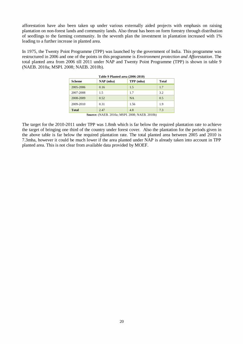
20

afforestation have also been taken up under various externally aided projects with emphasis on raising

plantation on non-forest lands and community lands. Also thrust has been on form forestry through distribution of seedlings to the farming community. In the seventh plan the investment in plantation increased with 1% leading to a further increase in planted area. In 1975, the Twenty Point Programme (TPP) was launched by the government of India. This programme was restructured in 2006 and one of the points in this programme is Environment protection and Afforestation. The total planted area from 2006 till 2011 under NAP and Twenty Point Programme (TPP) is shown in table 9

(NAEB. 2010a; MSPI. 2008; NAEB. 2010b).

Table 9 Planted area (2006-2010)

Scheme NAP (mha) TPP (mha) Total

2005-2006 0.16 1.5 1.7

2007-2008 1.5 1.7 3.2

2008-2009 0.52 NA 0.5

2009-2010 0.31 1.56 1.9

Total 2.47 4.8 7.3

Source: (NAEB. 2010a; MSPI. 2008; NAEB. 2010b)

The target for the 2010-2011 under TPP was 1.8mh which is far below the required plantation rate to achieve the target of bringing one third of the country under forest cover. Also the plantation for the periods given in the above table is far below the required plantation rate. The total planted area between 2005 and 2010 is 7.3mha, however it could be much lower if the area planted under NAP is already taken into account in TPP planted area. This is not clear from available data provided by MOEF.

21

3.2 Feasibility of afforestation

Afforestation/reforestation of wastelands requires huge investments. Balooni and Singh state in their paper that despite afforestation being economically feasible and ecologically sound, huge investment is needed for a large-scale afforestation. The costs are beyond the available means of most degraded landowners and other potential tree growers. On the other hand, the allocated budget of the Government for afforestation is far less

than the required budget (Balooni& Singh. 2003). The Indian government allocated 1% of its budget to the forestry sector between 1985-2002. Since, economic development has higher priority in India; an increase in government investment in the forestry sector is not likely to take place in near future. Balooni and Singh argue that institutional credit to facilitate investment in afforestation activities is necessary and this need has been recognized by the National Bank for Agriculture and Rural Development of India. Therefore, it has developed various schemes to finance individuals and

organisations for afforestation activities (Balooni& Singh. 2003). The same study also concludes that afforestation of wastelands in India are financially feasible without considering non-market benefits based on a review study on the economics of afforestation over the last two decades. It is believed that afforestation of wastelands is emerging as a big enterprise in India in order to meet the rising demand for raw materials of the rapidly growing wood-based industries. The reason behind this is the decline in supply of wood from government-owned forests in recent years due to conservation-oriented strategies of the government (Balooni& Singh. 2003).

Balooni reviews some studies on the economic performance of afforestation of wastelands in India. Most of the studies are focused on the west of the country (Balooni. 2003). Based on the review of these studies, it can be concluded that afforestation in the west and north of India is much more expensive compared to the east, central and south of the country. On the other hand, most of the studies were focused on west of the country the costs of afforestation cannot be compared fairly between the regions. The benefit/cost ratios for afforestation in all regions are above one and the Internal Rate of Return is higher than the discount rate.

Hence, it can be concluded that afforestation is economically feasible even in the arid and semi-arid regions of Rajasthan and Gujarat. According to a study by World Bank, the rate of return from afforestation investments by the government of India was low over the past decades. The given reasons for a low return were utilization of poor technology, low yield and the effective area of forest plantation on an average was only 60% of the gross planted area. Yet, plantation projects funded by external agencies were relatively well maintained during the first years after

establishment but after three years the plantations lacked maintenance and remained unprotected (MOEF. 2001c). In a midterm evaluation, NAP has been evaluated in 27 states of the country. The figure below shows the survival rate of the plantations in different bio-geographical zones of the country. As expected the survival rate in desert area and semi-arid area are the lowest compared to other bio-geographical zones, however the difference is not huge, see figure 3.

Figure 3 Average survival percentage in the sampled plantations for different bio-geographical zone


22

Figure 4 shows the survival rate of different models and as can be seen assisted regeneration has the highest

survival percentage, yet the difference between various models is quite small. However, the survival percentage decreases with the age of plantation.

Year-wise survival (%)

Figure 4 Year-wise survival under various models


Further it was concluded that in some of the Forest Development Agencies in Maharashtra, Madhya Pradesh, Orissa, Tamil Nadu, Uttar Pradesh, Uttarakhand, Goa and Karnataka plantation activities has been delayed and were behind the schedule due to lack of available wastelands in these states. Yet, according to WAI 2011 there exist million hectares of wastelands in these states, see table 32. Afforestation programmes in India have been undermined by widespread use of inappropriate and low quality seed that have led to plantation failure and poor growth which would discourage forest establishment in long

run. The Seed Development Scheme is meant to correct these problems. Where improved seed has been used eucalyptus yields increased from 7 to 20m 3ha-1year-1 (Williams. 2001). In the following paragraph example of few afforestation/plantation projects by government, NGO and private sector are given.

23

3.3 Small scale afforestation projects

Many small scale projects were carried out in the past to reclaim degraded land and the projects for which data was available is being discussed here. A 20ha plantation project was launched in Kolar district of Karnataka and the aim of this plantation was to rehabilitate wasteland through plantation. The project took place under the National Tree Growers’ Cooperative Federation. The aim of this federation is to restore and protect the

biological productivity of marginally productive and unproductive degraded/wasteland through a cooperative system. This federation organizes and develops village level Tree Grower’s Cooperative Society in the states of Andhra Pradesh, Gujarat, Karnataka, Orissa, Rajasthan and Uttar Pradesh. The national federation provides the village-level cooperative societies with plantation materials, financial assistance and conducts technical and socio-economic research and development activities (Balooni& Singh. 2003; MOEF. 2001a).

In Sisra Haryana, a small scale project started with the objectives to earn carbon credits from growing tree under Clean Development Mechanism Provisions of Kyoto Protocol, increase water holding capacity of the lands and humus of the soil, stabilising the sand dunes by converting the marginal and degraded croplands into forested lands and to create rural employment. The reclaimed area in this project borders the state of Rajasthan. The area is spread across eight villages comprising 370ha making use of seven forest species. In this area previous afforestation attempts under social forestry were not successful and without carbon finance

this project would not take place as it would be too costly. This project started in July 2008 and the credit period is 20 years with choice of renewal twice for 20 years. The verification takes place every five years which is followed by issuing of temporary Certified Emission Reductions (CIFOR. 2009; Green& Unruh. 2010; Chakraborty. 2010). The obstacles in this afforestation project were lack of access to credit, no access to planting material and technology since forestry is not the main land use in the region and absence of local organisations that focus

on tree plantation. A credit mechanism to give commercial loans to farmers to make long term investment possible was also missing and the plantation costs were beyond the farmer’s resource. Some of the barriers in the project were overcome as it is a Clean Development Mechanism project and through carbon credits the gestation period for economic returns of a project can decrease. Haryana Forest Department took this project as a small scale CDM pilot project to promote tree planting on degraded lands. The lands used for this project are lands affected by shifting sand dunes. According to initial assessment, the land used in this project would remain degraded if this small scale afforestation did not take place (CIFOR. 2009).

In 2001, the project Biomass Energy for Rural India (BERI) was started in Tumkur district of the southern state Karnataka and the project was supported by Global Environment Facility- United Nations Development Programme (GEF-UNDP). The project’s mission was to develop and implement a decentralized cost-effective, renewable bio-energy technology package to reduce GHG emission and at the same time meet rural

energy necessities. One of the bio-energy technology packages is the erection of the gasifier-units to produce electricity in order to meet the rural demand for electricity. The design of the project was based on research findings of the Indian Institute of Science’s Centre for Application of Science and Technology in Rural Areas. According to that research, biomass strategy based on sustainable forestry, biomass gasifier and systems can meet all the country’s rural energy demand and at the same time benefit the local and global environment by replacing fossil fuels and unsustainable wood as well reclaiming of degraded land (Ravindranath. 2011; BERI. 2009).

One of the important activities in BERI project was development of biomass on degraded forests. The plantation model, category of land used for plantation and its status are depicted in table10 (Ravindranath. 2011; BERI. 2009). As can be seen from the table, the scale of energy plantation for BERI project was very small. According to personal communication, one third of the plantation took place on wastelands, one third on underutilized forests and one third was based on farm forestry in semi-arid part of Karnataka state. The yield per ha was around 4.2 tonnes, but the harvested yield was lower due to stealing of biomass from the planted area. The project period was extended up to December 2010 (Srinivas. 2011).

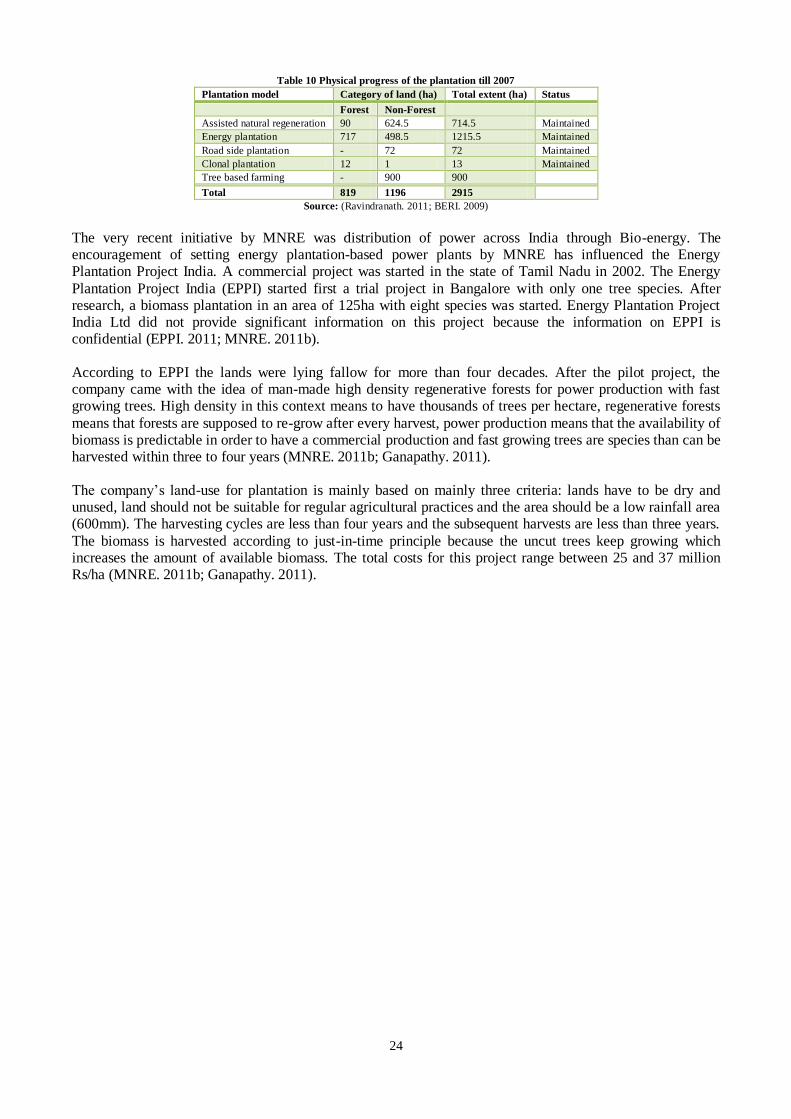
24

Table 10 Physical progress of the plantation till 2007

Plantation model Category of land (ha) Total extent (ha) Status

Forest Non-Forest

Assisted natural regeneration 90 624.5 714.5 Maintained

Energy plantation 717 498.5 1215.5 Maintained

Road side plantation - 72 72 Maintained

Clonal plantation 12 1 13 Maintained

Tree based farming - 900 900

Total 819 1196 2915

Source: (Ravindranath. 2011; BERI. 2009)

The very recent initiative by MNRE was distribution of power across India through Bio-energy. The encouragement of setting energy plantation-based power plants by MNRE has influenced the Energy Plantation Project India. A commercial project was started in the state of Tamil Nadu in 2002. The Energy

Plantation Project India (EPPI) started first a trial project in Bangalore with only one tree species. After research, a biomass plantation in an area of 125ha with eight species was started. Energy Plantation Project India Ltd did not provide significant information on this project because the information on EPPI is confidential (EPPI. 2011; MNRE. 2011b). According to EPPI the lands were lying fallow for more than four decades. After the pilot project, the company came with the idea of man-made high density regenerative forests for power production with fast growing trees. High density in this context means to have thousands of trees per hectare, regenerative forests

means that forests are supposed to re-grow after every harvest, power production means that the availability of biomass is predictable in order to have a commercial production and fast growing trees are species than can be harvested within three to four years (MNRE. 2011b; Ganapathy. 2011). The company’s land-use for plantation is mainly based on mainly three criteria: lands have to be dry and unused, land should not be suitable for regular agricultural practices and the area should be a low rainfall area (600mm). The harvesting cycles are less than four years and the subsequent harvests are less than three years.

The biomass is harvested according to just-in-time principle because the uncut trees keep growing which increases the amount of available biomass. The total costs for this project range between 25 and 37 million Rs/ha (MNRE. 2011b; Ganapathy. 2011).

25

3.4 Wasteland reclamation and bioenergy in Rajasthan

One of the afforestation projects in Rajasthan was the Aravalli Afforestation Project which took place between 1992 and 1997 and the project period was extended up to March 2000. The objectives of this project was to check desertification and to restore ecological status of the Aravalli hills by intensive reforestation; to meet the fuel-wood, fodder, grass timber and other forest products demand and to check soil erosion. The project took

place in ten districts of Rajasthan namely Alwar, Sikar Jhunjhunu, Nagpur, Jaipur, Pali, Sirohi, Udaipur, Chittorgarh and Banswara (Gov of Raj. 2013a; Yamashita et al. 2001; Shrivastava. 2007). The Aravalli Afforestation Project was funded by Japan and around 115000ha land was planted with the participation of local communities. In this project, not all objectives, like meeting the fuel-wood and fodder demand of the local, were achieved. However, as can be seen from table 11 the afforested area is somewhat larger than the initial targeted area (Gov of Raj. 2013a; Yamashita et al. 2001; Shrivastava. 2007).

Table 11 Aravalli Afforestation Project

Afforestation/Reforestation Activities Target (ha) Achievement

Reforestation of barren hills 25000 25400

Rehabilitation of degraded forests 101500 105930

Plantation on community land 19500 20060

Source: (Gov of Raj. 2013a)

The main goal of Aravalli afforestation project was to restore the ecological status of the Aravalli hills and not commercial plantation. One of the objectives of this study was to estimate the yield of biomass from plantation of wastelands. However, data on plantation of wastelands for bioenergy could not be found, except that plantation of Jathropha on wastelands is being promoted by the state government. Around 90% of

Jathropha in India is being grown in the state of Rajasthan and the state government offers free Jathropha saplings and fallow land on very nominal lease (Gov of Raj. 2013b; Pandey et al. 2010; Herath et al. 2011). Among non-conventional energy sources, biomass has a good potential for electricity generation in the state of Rajasthan. To promote renewable power, the government of Rajasthan promulgated a policy in 1999 known as Policy for Promoting Generation of Power through Non-Conventional Energy Sources. This policy ended in 2004 and the government issued a comprehensive policy for promoting generation of electricity through

non-conventional energy source, which is known as Policy-2004. The state also decided to issue a comprehensive policy for generation of electricity from various sources to offer solution to various problems faced by developers, investors and utilities (Gov of Raj. 2010; Gov of Raj. 2004). In 2010, the state government issued another policy namely, Policy for Promoting Generation of Electricity from Biomass 2010. In this policy Biomass means forestry based & agro-based industrial residues, energy plantations, forestry and agro- residues. There are eight existing biomass based power plants in Rajasthan, but

only four of these power plants are operating. In addition, there are six biomass power projects under process of installation (Gov of Raj. 2010; Gov of Raj. 2004).

26

3.5 Discussion

Based on the study of Balooni and Singh discussed in previous paragraph, afforestation of wastelands is economically feasible. However nationally implemented programmes like Joint Forest Management failed due to low returns from the plantations. The main reasons were lack of complementarily between site and species, poor seeds, nursery techniques and quality of the stock. Despite having large plantation programmes, India

lacks a system for suitable collection, testing, classification, certification and safe storage of tree seeds up to now. According to World Bank observation, in case of teak plantation only 15% of planting material was good enough for plantation (Palm. 2011; MOEF. 2001c). Other reason for failure of forestry programmes were insufficient site preparation, poor plantation establishment practice, and lack of after-establishment maintenance. In case of externally aided projects, the plantations are well established, but the maintenance diminishes with time. This means that a well-established

project might be unsuccessful after a few years leading to loss of the entire investment. Also, illegal removals, absence of people’s participation, and poor protection from fire and grazing contributed to poor state of the forest plantations. Lack of infrastructure such as roads, land use conflicts, budgetary constraints, monitoring and evaluation, and insufficient research and development support also played a role in failure of plantation projects (Palm. 2011; MOEF. 2001c).

An environmental barrier like scarcity of water is another major problem in establishment of plantations, especially plantation of degraded lands. The areas where these lands are located have become drier and warmer. The available irrigation-water is required for the agriculture and an environmental barrier like scarcity of water is difficult to overcome. The suggested solution is plantation of species that do not require much

water and nutrient and at the same time increase the organic material of the soil and limits the erosion of wastelands (Palm. 2011). Another issue regarding afforestation of degraded lands was unsuitability of land for plantation. In many cases the degraded lands that were used for plantation, were identified as extremely degraded. Despite that the plantations were carried out to meet the target of covering one third of the country with forests (MOEF. 2001c; Damodaran& Engel. 2003).

Projects regarding afforestation of degraded lands are also hindered by economic constraints (Balooni& Singh. 2003; Ravindranath& Hall. 1995). The environmental and socio-economic benefits of afforestation are quite clear for the local stakeholders and they are willing to invest their time and give their land to an eventual

project. However, local financial supports are missing and besides the policies are fragmented across numerous agencies with different policy mandates. Also, due to absence of trained personnel and comprehensive database, many projects are delayed (Ministry of Finance.; MOEF. 2001b).

According to Palm et al 2010, a compensatory scheme for increasing carbon stock and vegetation cover could be a possible option to overcome financial barriers and rehabilitate more wasteland areas and at the same time generates income for the locals. Palm points out that the price of forest carbon credits needs an improvement and since afforestation of wasteland benefits the public good, national means or international aid should cover the costs of it. Failure of nationally implemented programmes like Joint Forest Management Programme is

assigned to low returns from the plantations. Therefore, Palm states that a financial return either from carbon sequestration or payment for the environmental services will stimulate communities and local institutions to be active in the maintenance of the wasteland rehabilitation programmes (Palm. 2011; MOEF. 2001c).

Despite the fact that many schemes with similar goals were brought under National Afforestation Programme, lack of clarity still exist and other programmes like Green India Mission with similar goal exist next to NAP. In order to specify the role of afforestation in future, it is essential to specify the role of each plantation that has taken place in India. Therefore, Plantations that have been taken place in India need to be brought in a clear picture. An inventory of the past and existing plantations is necessary with detailed data on costs

nationally and externally aided afforestation projects. Having a clear picture of past and current plantation project with cost and yield details will give a much clear picture of feasibility of afforestation for different agro-climatic zones.

27

3.6 Summary

Utilization of fuel-wood by households and high population density have contributed significantly to deforestation in India. The government, private sector and foreign agencies have come up with numerous

attempts to stop deforestation and instead stimulate afforestation. The National Forest Policy in 1894 was the first move of the government to tackle this problem by stressing on conservation of forests in order to meet the basic needs of communities living at the forest fringes. The National Forest Policy was the forerunner of the green movement in India. In 1952, the policy was revised and the new policy emphasized on the extension of forests beyond the established forest areas. The objectives were to bring 33% of the total geographical area under tree cover by

2012, preserving the remaining natural forests and checking the extension of sand dunes in the desert areas. This has led towards social and agro/farm forestry. Due to extreme depletion of forest resources the policy was adjusted in 1988. The new evolved strategy in the policy of 1988 was the participation and involvement of communities in protection and regeneration of forests. Actual afforestation/reforestation started in the late 1950s. The activities were carried out under different programmes. The main objectives of these programmes were conserving the environment to meet the wood

demand by planting fast growing species suitable for fuel-wood and timber. Externally aided social forestry projects were also implemented during 1980-1992 with the same objectives by targeting degraded forests. Community-land plantations have also been launched outside forest reserves on wastelands owned by the government and privates. As part of rural and wasteland development programmes, large-scale plantations and social forestry projects were launched in several states in the early 1980s. Monitoring and Evaluation scheme, and Support to Regional Centres scheme started in 1988-89 under National Afforestation and Eco-development Board

(NAEB). The aims of these programmes were to evaluate sanctioned projects, to disseminate technologies and programmes and conduct studies relevant to afforestation and eco-development. Joint Forest Management (JFM) scheme was introduced by MOEF in 1990. NAEB started afforestation programme to support JFM in 1992. Grants-in-Aid for Greening India is another scheme under NAEB which was started in 2005-2006. The objective of this project was to increase environmental capacity by planting trees, establishing high-tech nurseries, create awareness for use of improved technology and planting material

and increase tree cover through planting of non-forest lands. The Green India Mission under the National Action Plan on Climate Change was initiated in 2011 with the objectives to increase forest cover on 5mha of forest/non-forest lands, improve quality of forest cover on another 5mha, and enhance annual CO2 sequestration of 50-60 million tonnes by the 2020. Green India Mission also supports programme of nurseries for raising quality seedlings to meet the demands of farmers.

The Twenty Point Programme (TPP) was also launched by the government of India in 1975. Environment protection is one of the twenty points aimed by this programme. TPP was restructured under nine five-year plans in 2006. All the efforts resulted to afforestation of almost 35mha land from 1950 to 2005. In addition an area of 7.3mha was planted since the establishment of TPP in 2006. The average annual plantation rate between 1980 and 2005 was 1.32mha and the target annual plantation rate for 2010-2011 under TPP was 1.8mha per year. The annual plantation rate was and still is below the required plantation rate to bring one third of the country under

forest cover.

Supply of wood from government-owned forests have been declining that is why it is believed that afforestation of wasteland is emerging as a big enterprise in India to meet the demand of wood-based industries. However, from commercial point of view economical feasibility of afforestation is one of the most important factors for the businesses. Consistent with a study on economic performance of afforestation, afforestation of wastelands is financially feasible, even without taking non-market benefits into account.

28

According to a study by World Bank the rate of return on the investments made on afforestation by Indian

government over the past decades was low. The reasons for low return were utilization of poor technology, low quality seed, low yield and lack of maintenance. Even if afforestation is economically feasible, huge investments are needed for large-scale afforestation of wastelands. Institutional credit to facilitate investment in afforestation activities were considered necessary. Therefore, the National Bank for Agriculture and Rural Development of India has developed various schemes to finance individuals and organisations for afforestation undertaking.

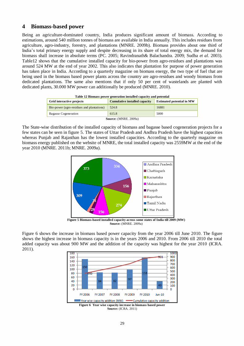
29

4 Biomass-based power

Being an agriculture-dominated country, India produces significant amount of biomass. According to estimations, around 540 million tonnes of biomass are available in India annually. This includes residues from agriculture, agro-industry, forestry, and plantations (MNRE. 2009b). Biomass provides about one third of India’s total primary energy supply and despite decreasing in its share of total energy mix, the demand for biomass shall increase in absolute terms (PC. 2005; Ravindranath& Balachandra. 2009; Sudha et al. 2003).

Table12 shows that the cumulative installed capacity for bio-power from agro-residues and plantations was around 524 MW at the end of year 2002. This also indicates that plantation for purpose of power generation has taken place in India. According to a quarterly magazine on biomass energy, the two type of fuel that are being used in the biomass based power plants across the country are agro-residues and woody biomass from dedicated plantations. The same also mentions that if only 50 per cent of wastelands are planted with dedicated plants, 30.000 MW power can additionally be produced (MNRE. 2010).

Table 12 Biomass power generation installed capacity and potential

Grid interactive projects Cumulative installed capacity Estimated potential in MW

Bio-power (agro-residues and plantations) 524.8 16881

Bagasse Cogeneration 615.8 5000

Source: (MNRE. 2009a)

The State-wise distribution of the installed capacity of biomass and bagasse based cogeneration projects for a few states can be seen in figure 5. The states of Uttar Pradesh and Andhra Pradesh have the highest capacities whereas Punjab and Rajasthan has the lowest installed capacities. According to the quarterly magazine on biomass energy published on the website of MNRE, the total installed capacity was 2559MW at the end of the year 2010 (MNRE. 2011b; MNRE. 2009a).

Figure 5 Biomass-based installed capacity across some states of India till 2009 (MW)


Figure 6 shows the increase in biomass based power capacity from the year 2006 till June 2010. The figure shows the highest increase in biomass capacity is in the years 2006 and 2010. From 2006 till 2010 the total added capacity was about 900 MW and the addition of the capacity was highest for the year 2010 (ICRA. 2011).

Figure 6 Year wise capacity increase in biomass based power

Source: (ICRA. 2011)

30

4.1 Biomass potential from wastelands

A nationwide Biomass Resource Atlas project, Biomass Resource Atlas of India (BRAI), was executed by Combustion, Gasification & Propulsion Laboratory on behalf of MNRE with a view to assess the biomass availability in order to estimate the power generation potential. The availability of biomass, excluding the current usage such as fodder, domestic fuel, thatching and manure, was assessed. The available biomass

resources in this project are for 2000 to 2004. Initially the atlas contained data on agro-residues, but later it included biomass potential from forests and wastelands. In this project the aim was to develop a software package for the estimation of power generation potential. In order to get some specific field data and the local trend in the utilization of biomass, taluk9 and district level surveys were conducted (CGPL10. 2011; CGPL.; MNRE. 2012). The Biomass Resource Atlas of India has considered wasteland as extension of forests for their assessment of

biomass potential from wastelands. The first level estimations are based on the available species in the forest. For each state, the distribution of species is considered the same, consequently the area will be the same for each class of forest and the yield of residues are used for the estimation of biomass potential from wastelands (CGPL.; CGPL. 2010).

Table 13 State-wise biomass potential from wastelands

State Area (mha) Biomass Generation

(Mt/year)

Biomass Surplus

(Mt/year)

Power Potential

(MWe)

Maharashtra 7.44 1.08 7.32 1.02

Gujarat 7.73 10.68 7.18 1.01

Madhya Pradesh 7.33 10.34 6.90 0.97

Jammu & Kashmir 6.89 8.16 5.38 0.75

Rajasthan 10.98 6.70 4.42 0.62

Andhra Pradesh 2.80 4.14 2.80 0.39

Chattisgarh 1.69 2.39 1.59 0.22

Uttar Pradesh 1.56 2.22 1.49 0.21

Karnataka 1.50 2.16 1.43 0.20

Jharkand 1.08 1.57 1.05 0.15

Arunachal Pradesh 0.92 1.15 0.84 0.12

Himachal Pradesh 0.90 1.19 0.79 0.11

Tamil Nadu 0.69 1.15 0.76 0.11

Assam 0.65 0.87 0.57 0.08

Bihar 0.40 0.58 0.39 0.05

Mizoram 0.45 0.55 0.37 0.05

Tripura 0.29 0.40 0.26 0.04

Haryana 0.24 0.33 0.22 0.03

Meghalaya 0.22 0.27 0.18 0.03

Manipur 0.19 0.22 0.15 0.02

Punjab 0.05 0.12 0.08 0.01

Sikkim 0.07 0.09 0.06 0.01

Orissa 0.05 0.09 0.06 0.01

Nagaland 0.06 0.08 0.05 0.01

West Bengal 0.03 0.04 0.03 0.00

Uttaranchal 0.01 0.02 0.01 0.00

Kerala 0.01 0.01 0.01 0.00

Total 54.25 66.35 44.37 6,21

Source: (CGPL. 2011)

The state-wise power potential from wastelands and biomass surplus is given in table 13. As can be seen, Maharashtra, Gujarat, Madhya Pradesh, Jammu & Kashmir and Rajasthan have the highest power potential from wastelands. Although the states of Rajasthan and Jammu & Kashmir have the largest wasteland area

compared with the other afore mentioned states, the power potential in these two states are lower than those states. This is mainly because these two states have large areas of uncultivable wastelands. Unlike the WAI where the wastelands are given district-wise, the BRAI provides biomass power potential from wasteland on taluk level (CGPL. 2011; CGPL. 2010).

9 An administrative district for taxation purposes typically comprising a number of villages (OALD. 2011).

10

Combustion, Gasification & Propulsion Laboratory, Department of Aerospace Engineering Indian Institute of of Science

31

Table 14 Capital cost and load factor

Capital cost Rs Crore/MW Plant load factor%

Biomass 5 - 5.5 50 - 80

Wind 6 - 6.5 15 - 30

Small Hydro 6 - 7 25 - 70

Solar PV 14 - 15 20

Source: (ICRA. 2011)

The total power potential from wastelands is around 6211 MW, while the installed capacity as mentioned earlier was only 2259MW at the end of 2010. Based on the previous tables and figures it can be concluded that India has high potential for biomass based power, while the installed capacity is very low. Compared to other renewable energy sources, the load factor of a biomass based power plant is much higher and also the capital cost for biomass based power plant is much lower, see table 14.

4.2 Prosopis juliflora

Climate is one of the important factors in afforestation activities. India has various climate conditions and the climate of Rajasthan is arid in the west and semi-arid in the east of the state. The costs of plantation are dependent on many factors like quality of the soil and its nutrient value, rainfall, and the requirement of vegetation to be planted. Therefore the energy crops have to fulfil certain conditions. The most important conditions are to survive under unfavourable biotic conditions like low rainfall and low input of management. An indicator to survival is the yield of biomass. The very important factors for a plant species to be used as

energy source are the growth rate, calorific value of the wood and suitability of the species to local climate (Sudha et al. 2003; Sharma. 1992). In table 41 the tree species for different annual rainfall is depicted. Prosopis juliflora and Acacia tortilis can be planted in different rainfall zones of the country as can be seen from table 15 (MOEF. 2001a; CAZRI11. 2009). .

Table 15 Tree species for different rainfall regions

Annual rainfall zone (mm) Trees species

150 - 300 Prosopis juliflora, Acacia tortilis, Acacia senerged

300 - 400 Acacia tortilis, Acacia Senegal, Prospis juliflora, Prosopis cineraria, Tecomella undulate,

Parkinsonia aculeate, Acacia nubica

400 - 550 Acacia tortilis, Prosopis cineria Prosopis juliflora, Acacia Senegal, Dalbergia sissoo

Source: (MOEF. 2001a; CAZRI. 2009)

Prosopis juliflora has the character of adapting to different soils and landscapes, also in arid and semi-arid environments where the rainfall is quite low. Prosopis juliflora had been used wildly for reclamation of degraded land in the arid and semi-arid parts of India. This tree species has a calorific value between 4200-4800 kcal kg-1. Prosopis species coppice well and do not show any detrimental effects on the plant health after repeated cutting. The tree does not require special care, therefore can be planted on marginal and wastelands. The tree does not only give high quality fuel-wood, but also by-products like timber, forage and honey. Under

favourable condition, the yield of Prosopis juliflora is said to be very high, however different studies give different yield for this species (Pasiecznik et al. 2001; Singh. 1998; DFID et al. ; Wright. 2010). The reported yields range from 0.5t/ha/year to 39t/ha/year and vary per region. The yield for India is between 11-20t/ha/year and yield as low as 0.6-1.8t/ha/year has also been reported, see table 16. These low yields are usually obtained from arid regions of India where the mean annual rainfall is below 300m and with no irrigation or post-planting care. The highest yield was obtained from a trial in a region in Kenya where the

annual rainfall is above 1500 mm. The plants were also provided additional water and post-planting maintenance. The expected biomass yield over a 5-10 year rotations is said to be generally in the range of 2-8t/ha/year for plantation densities of 400-2500 trees/ha in a mean annual rainfall zones of 400-800 mm without any additional irrigation. Annual biomass production per tree is also reported for different regions. In Somalia, individual biomass increments for Prosopis juliflora include 0.2-1.7 kg/tree/year, 4.9-8.4 kg/tree/year in India and up to 10 kg/tree/year in Pakistan (Pasiecznik et al. 2001).

11

Central Arid Zone Research Institute

32

Table 16 Reported yield of Prosopis juliflora in literature

Country Yield t/ha/year Yield m3/ha/year Source

USA 7-20 Felker et al 1983

Kenya 6-12 Kaarakka and Johansson 1992

India 11-20 Chaturvedi and Behl 1996

Ethiopia 10-16 Abebe 1994

Sudan 1.6 Wunder 1999

India 0.6-1.8 Singh et al 1990

Source: (Pasiecznik et al. 2001)

Yields of around 50 to 60 tonnes per hectare for 10 year old plantation and 75 to 100 tonnes per hectare after 15 years have also been reported. In Gandhinagar Gujarat, the yield of dry fuel-wood for a four yield old

plantation with a density of 6410 plants per hectare was around 148 tonnes (Saxena. 1998; Singh. 2008). The depicted data in table 17 shows the yield for Prosopis juliflora for sandy soils from trials in arid part of Rajasthan (FAO. 1985). It is not mentioned whether the yields are dry weight or fresh weight, but assuming that the given yields in table 43 are fresh weight, they are still much higher than the estimated yield of 5 and 9 kg per tree for Barmer and Churu respectively. On the other hand, lower average yields of 4.3 and 1.5 kg per tree for 5 year old trees for the districts of Bikaner and Barmer and 27 kg per tree for 10 year old trees for

Jhunjhunu have also been reported (Saxena. 1998).

Table 17 yield Prosopis juliflora in sand dunes of Rajasthan

Yield (kg)

Jhunjhunu Churu Bikaner Gadra Road Sardarshahr Churu

Age tree

4 - - 15,1 15,5 41,9

5 - - 23,9 41,7 36,7

6 - - - 43,8 36,2

7 78,8 - - - 38,2

8 193,3 - - - 49,8

9 51,6 47,5 - - 41,5

10 136,9 - - - 54,4

Source: (FAO. 1985)

Prosopis juliflora gives high quality fuel-wood and charcoal and useful by-products like timber, forage and

honey. However, it can become an invasive species and therefore the management of the species should be with care. It grows fast and has a deep to very deep root system. The tree can also be planted on marginal and wasteland for reclamation purpose as the tree does not require special care (Saxena. 1998; Sirmah et al. 2008).

33

4.3 Summary

According to estimations around 540 million tonnes of biomass are available in India annually. This includes residues from agriculture, agro-industry, forestry, and plantations. Biomass provides about one third of India’s

total primary energy supply. Despite decreasing in its share of total energy mix, the demand for biomass shall increase in absolute terms. Two types of fuel: agro-residues and woody biomass from dedicated plantations are mainly being used in biomass based power plants across the country. This indicates that plantation for purpose of power generation has been taking place. The total installed biomass-based capacity was 2559MW at the end of 2010. The states of Uttar Pradesh and Andhra Pradesh have the highest installed capacities whereas Punjab and Rajasthan have the lowest installed

capacities. To estimate the power generation potential, a nationwide Biomass Resource Atlas project (BRAI) was carried out to assess the biomass availability excluding the current usage. The available biomass resources in this project are from 2000 to 2004 and contain data on agro-residues and biomass potential from forests and wastelands as extension of forests. Despite the fact that Rajasthan and Jammu & Kashmir have the largest wasteland area, the power potential from wastelands is lower than the states of Maharashtra, Gujarat and Madhya Pradesh because these two states have large areas of uncultivable wastelands. The total power potential from wastelands is according to BRAI around 6211 MW.

Energy crops for plantation in wastelands must have certain attributes to survive in low rainfall region, low nutrient value and low soil quality land. Prosopis juliflora and Acacia tortilis can be planted in different rainfall zones of India. Prosopis juliflora is adapting to different soils like arid and semi-arid environments, provides high quality fuel-wood and charcoal. It also produces useful by-products like timber, forage and honey. It grows fast and has a deep to very deep root system. This plant has been used wildly for reclamation of degraded land in the arid and semi-arid parts of India. This tree species has a calorific value between 4200-4800 kcal kg-1. Prosopis species coppice well and do not show any detrimental effects on the plant health after

repeated cutting. The tree does not require special care however; it can become an invasive species which needs careful management. The yields of Prosopis juliflora range from 0.5t/ha/year to 39t/ha/year depending on the region. The yield of this plant is between 11-20t/ha/year in India. Nevertheless low yield of 0.6-1.8t/ha/year has also been reported. Low yields are usually obtained from arid regions of India where the mean annual rainfall is below 300ml without irrigation or post-planting care.

34

5 Methodology

An exploratory research was conducted to find literature on afforestation/plantation in India, in particular plantation of wasteland with energy crops. Interviews were conducted to gain more insight in availability of wastelands, rehabilitation of wastelands, and their current use. In the following paragraphs the methodology for state and wasteland selection; yield estimation; the economic performances of biomass plantation; and the performance of biomass supply chains are described separately. All the data used in this study are presented in

paragraph 1.3 and Appendices.

5.1 State and wasteland selection

Most recent data on the extent and type of wasteland, presented in Wasteland Atlas of India 2011 (WAI), were used to estimate the potential of biomass from wasteland. The suitability of different wasteland categories for plantation is depicted in table 3 which is determined with data presented table 18 and 19. In table 20 wastelands are divided into four categories namely suitable, moderately suitable, marginally suitable and unsuitable. Data presented in table 18 is taken from IIED (2010)12, which is in turn taken from WAI 2005,

wherein the wastelands were categorized into suitable, moderately suitable and unsuitable categories.

Table 18 Suitability of different wasteland categories for plantation

Category of wasteland Suitability Category of wasteland Suitability

1 Gullied and/or ravenous land (Shallow) Sa

15 Sands-(Levees) Mods

2 Land with scrub suitable S 16 Sands-(Coastal Sand) Mods

3 Land without scrub suitable S 17 Sands-(Semi Stab.-Stab.>40m) moderately Mods

4 Land affected by salinity/alkalinity (Slight) S 18 Sands-(Semi Stab.-Stab Moder. High 15-40m) Mods

5 Shifting cultivation area (Abandoned Jhum) S 19 Sands-(Semi Stab.-Stab. Low<15m) Mods

6 Shifting cultivation area (Current Jhum) S 20 Sands-(Closely Spaced Inter-Dune Area) m Mods

7 Underutilized/degraded notified forest land S 21 Mining wastelands Mods

8 Underutilized/degraded notified forest land

(Agri.) S 22 Industrial Wastelands Mods

9 Degraded pastures/grazing land suitable S 23 Gullied and/or ravenous land (Deep) Unsc

10 Degraded land under plantation crop S 24 Waterlogged and Marshy land (Permanent) Uns

11 Gullied and/or ravenous land (Medium) Modsb

25 Sands-(Flood Plain) Uns

12 Waterlogged and Marshy land (Seasonal) Mods 26 Barren Rocky/Stone Waste/Sheet Rock Area Uns

13 Land affected by salinity/alkalinity (Strong) Mods 27 Steep Sloping Area Uns

14 Land affected by salinity/alkalinity (Moderate) Mods 28 Snow covered and/or Glacial Area Uns

aS-suitable, bMods-Moderately suitable, cUns-Unsuitable

Source: (International Institute for Environment and Development. 2010)

In WAI 2005, wastelands are divided in 28 categories, however in WAI 2011 some categories are merged together and divided into 23 categories. Table 19 is taken from Ministry of New and Renewable Energy (MNRE) (2010)13 wherein the suitability of wastelands for Prosopis juliflora and high yield plantation is discussed. Based on data depicted in table 19, barren rocky areas are suitable for plantation of Prosopis

juliflora. However, according to IIED, barren rocky wasteland is not suitable for energy plantations, see table 18. Further, in table 19 wasteland categories open scrubland and dense scrubland are not considered suitable for plantation because these wasteland categories are used for grazing. Yet according to the definition of wasteland, see chapter 2, wasteland is land that is underutilized.

12

Biomass energy-optimising its contribution to poverty reduction and ecosystem service, IIED 2010 13

Dedicated Energy Plantation and Forest Residues, MNRE 2010

35

Table 19 Suitability of different wasteland categories for plantation

Category Pj Hy Remarks

1 Gullied and/or ravenous land-Medium Yes Yes

2 Gullied and/or ravenous land deep/very deep ravine No No Water logged in monsoon season, therefore unsuitable

3 Land with dense-scrub No No Used as pasture, therefore should not be considered

4 Land with open-scrub No No Same as above

5 Waterlogged and Marshy land-Permanent No No Plantation in waterlogged area not possible

6 Waterlogged and Marshy land-seasonal No No Same as above

7 Land affected by salinity/alkalinity-moderate Yes Yes

8 Land affected by salinity/alkalinity-strong Yes No Strong saline/alkaline not suitable for high yield plantation

9 Shifting cultivation area- current Jhum No No Cultivation area cannot be considered for energy plantation on account

of food security

10 Shifting cultivation area-abandoned Jhum No No Same as above

11 Under- utilized/degraded forest-scrub dominated Yes Yes

12 Agricultural land inside notified forest land No No Same as above

13 Degraded pastures/grazing land No No As used for pasture it provides fodder for cattle

14 Degraded land under plantation crops Yes Yes

15 Sands-Riverine Yes Yes

16 Sands- Costal sand Yes No High yield plantation cannot be grown in sandy soil

17 Sands-Desert Sand Yes No Same as above

18 Sands-Semi-stabilized to stabilized (>40m) dune Yes No Same as above

19 Sands- Semi-stabilized to stabilized moderately high

(15-40m) dune Yes No Same as above

20 Mining wastelands No No Productive soil is eroded, hence cultivation not possible

21 Industrial wastelands No No The land is private thus difficult to get it for plantation

22 Barren rocky area Yes No Minimum rainfall for high yield 800mm, thus not suitable

23 Snow cover and/or glacial area No No Plantation cannot be grown in snow

aPj-Prosopis Juliflora, bHy-High yield


Around 57% of wasteland consists of categories land with dense scrub, land with open scrub14 and degraded forests15 (3, 4 and 11) and these categories are considered suitable. Wasteland categories sand dunes16 and sand-desertic17 (17, 18 and 19) form around 6% of total wasteland area and are marginally suitable. Other suitable, moderately and marginally suitable wasteland categories have much smaller area, as discussed in

chapter 2. One of the aims of this study was to estimate the biomass potential from the most suitable wasteland categories, therefore presence of wasteland categories land with dense scrub, land with open scrub and degraded forest land, and their extent was one of the criteria for state selection. Wasteland can be found in all states of India, however estimating the biomass potential for the whole country was beyond the scope of this study. Figure 7 shows which criteria were used for the state selection and figure 8 shows which state was selected in the third step.

14

These categories are also referred as scrub land or land with scrub in this report 15

For the sake of simplicity wasteland category Under- utilized/degraded forest-scrub dominated (11) is referred as degraded forests in this report 16

Semi-stabilized to stabilized dunes with > 40m height and dunes with height between 15 and 40m 17

Also called Sand –Desert sand

36

Table 20 Wasteland categories according WAI 2011

Wasteland Category Wasteland Category

1 Gullied and/or ravenous land-Medium Unsa

13 Degraded pasture/grazing land S

2 Gullied and/or ravenous land-Deep/very deep ravine Uns 14 Degraded land under plantation crops S

3 Land with dense scrub Sb

15 Sands-Riverine Mods

4 Land with open scrub S 16 Sands-Coastal sand Mods

5 Waterlogged and Marshy land-Permanent Uns 17 Sands-Desert Sands Mars

6 Waterlogged and Marshy land-Seasonal S 18 Sands-Semi-stabilized to stabilized (>40) dune Mars

7 Land affected by salinity/alkalinity-Moderate Modsc

19 Sands-Semi-Stabilized to stabilized moderately high (15—40m) dune Mars

8 Land affected by salinity/alkalinity-Strong Marsd

20 Mining Wasteland Mars

9 Shifting cultivation area-Current Jhum S 21 Industrial Wasteland Mars

10 Shifting cultivation area-Abandoned Jhum S 22 Barren rocky area Uns

11 Underutilized/degraded forest-scrub dominated S 23 Snow cover and/or glacial area Uns

12 Agricultural land inside notified forest land S

a Uns-Unsuitable, b S-suitable, c Mods-Moderately suitable, d Mars-Marginally suitable


Figure 7 criteria for the state choice

The three states with highest component of wasteland are Rajasthan, Jammu & Kashmir and Madhya, see table 5. Jammu & Kashmir has the smallest area in the categories mentioned in figure 2 and therefore is excluded in the second step. The state with lowest forest cover is Rajasthan, thus Madhya Pradesh is excluded. The selected state is Rajasthan with highest component of wasteland and lowest forest cover per capita, see

figure 8.

Figure 8 State selection

37

5.1.1 Study area

The potential of biomass from wastelands economic performance of energy plantation and the performance of biomass supply chain were determined for 32 districts of the state Rajasthan. To estimate the biomass potential for all the states of India was beyond the scope of this study. With 18.2% of total wasteland area,

Rajasthan has the largest wasteland area in India; therefor this study was limited to Rajasthan. Additionally, Rajasthan has the lowest forest cover per capita in India. The biomass potential was determined for all districts of Rajasthan. The economic performance of selected supply chains were only estimated for districts with either coal based or biomass based power plant. The location of large scale biomass power plant was determined by biomass potential from wasteland and cost of production of biomass. Since the state of Rajasthan was selected as study area, the biomass potential was not only estimated for the

most suitable wasteland categories but also for categories sand-dunes and sands-desertic (17-19), because Rajasthan has large areas of wasteland available in the last mentioned categories, see table 4-5 for category-wise and state-wise wasteland area, and Appendix I for district-wise wasteland area. In the next subparagraph the methodology used for yield estimation of Prosopis juliflora from six wasteland categories is described.

5.2 Yield estimation

From literature study data was gathered on suitable species for plantation of wasteland. Prosopis juliflora was selected as suitable species for the arid and semi-arid climate of Rajasthan. The characteristics of Prosopis

juliflora is described in paragraph 2 of chapter 4. The method to determine the yield of Prosopis juliflora is based on the method described in Wicke et al (2011)18 and Vashev et al (2010)19 for estimating the potential of bioenergy from salt affected soils. However, the method was modified to apply it on other wasteland categories other than salt affected soil and to estimate the potential without using GIS. The method required certain region specific soil, terrain and climate characteristics. The used software’s and sources for soil and terrain, and climate requirements are depicted in table 21. The soil and terrain, and climate requirements are depicted in table 5 and 15. In 1.3 and Appendices all the tables with data used for the methodology can be found.

Table 21 Used sources and programmes

Requirements Software Database Source

Soil and terrain

characteristics HWSD viewer

Food and Agriculture Organization Land

Resources

Soil organic carbon Soil health map Rajasthan Krishi Government of Rajasthan

Slope Web-GIS maps Web GIS India-WRIS Web GIS

Groundwater depth Web-GIS maps Central Ground Water Board, India; India-

WRIS Web GIS

Climate requirements New_LocClim New LocClim Food and Agriculture Organisation

Area soil mapping unit Interactive Digital Soil Map of the

World GeoNetwork Food and Agriculture Organisation

Administrative layer Bhuvan Thematic Data National Remote Sensing

Centre

National Remote Sensing Centre Government of

India

The yields of forestry plantations on salt affected soils used by Wicke et al (2011) and Vashev et al (2010) matches climate, soil, and terrain requirements of tree species with the characteristics of the land under consideration. The following (groups of) land characteristics are distinguished with respect to soil and terrain:

topography (slope gradient) wetness (internal drainage class) physical soil characteristics (gravel content, drainage class, soil texture class, gypsum, calcium

carbonate content) chemical soil characteristics (cation exchange capacity of the clay fraction, base saturation, total

exchangeable bases, organic carbon, pH (H2O)) degree of salinity–alkalinity (electrical conductivity, exchangeable sodium percentage)

18

The global technical and economic potential of bioenergy from salt-affected soils, Wicke et al 2011 19

Biosafar Project Deliverable 9: Cropping Potential For Saline Areas in India, Pakistan and Bangladesh, Vashev et al 2010

38

Vashev et al. include three additional land characteristics (flooding, soil depth, and depth of

groundwater) for which global data are unavailable or insufficient to be able to include them in the global analysis. In addition to land characteristics, the following climatic characteristics are taken into account:

rainfall (annual precipitation, length of dry season) temperature (mean maximum temperature of the warmest month, mean minimum temperature of the

coldest month, mean annual temperature) radiation (fraction of sunshine hours).

Depending on the tree-specific requirements, ratings between 0 (unsuitable) and 100 (very suitable) are

defined, indicating the level of limitation for the growth of the tree species under the given climate and land characteristics. A climate index and a soil and terrain index are then calculated based on the theory that the scarcest resource is the limiting factor for plant growth.

5.2.1 Soil

The soil parameters for Rajasthan are extracted from Harmonized World Soil Database (HWSDB), except soil organic carbon level which is extracted from soil health database of Rajasthan20. HWSD provides a much higher organic carbon level, while the organic carbon level provided by soil health data base gives a much lower carbon level and is also up to date. Rajasthan has 23 different soil mapping-units21 which in turn can

have up to 9 soil unit/topsoil texture combinations. Figure 9 shows the soil map of Rajasthan which was constructed by adding shape files of the state and districts of Rajasthan with their names. Every colour within the district represents a soil mapping unit and as can be seen, most of the districts have more than one soil mapping unit. The soil mapping units of Rajasthan with its characteristics and district-wise soil mapping units are depicted in Appendix II and III.

Figure 9 Soil map of Rajasthan district-wise

Source: (FAO et al. 2012)

In order to rate the soil parameters, an administrative layer of India was added to Digital Soil Map of the World22 and for each district of Rajasthan, the area of every soil mapping unit was measured. Subsequently,

20

Krishi Rajasthan, Government of Rajasthan, 2011 21

A soil map unit is a collection of areas defined and named the same in terms of their soil components or miscellaneous areas or both. HWSD provide

soil data at about 1kmx1km. 22

http://www.fao.org/geonetwork/srv/en/main.home

http://www.fao.org/geonetwork/srv/en/main.home

39

the percentage of every soil mapping-unit was calculated and also within every soil mapping-unit the

percentage of soil units was estimated. The soil units of all soil mapping-units were rated and for soil mapping-units with more than one soil unit, each soil unit was rated separately and a weighted average was used. Figure 10 shows the steps and assumptions for rating the soil parameters.

Figure 10 Soil rating

HWSD contains physical and chemical characteristics of topsoil as well of subsoil for every soil unit. To rate the soil units, data on physical and chemical characteristics of topsoil was used. The organic carbon level, which is extracted from soil health database of Rajasthan, is provided per village. The number of villages for different organic carbon ranges given in table 23 was counted and rated. Subsequently, a weighted average of these ranges was used for organic carbon level of wasteland categories land with scrub and degraded forests. Some of the districts have more than two thousand villages. Therefore,

the amount of data for 32 districts is too large to be added in this report. Figure 11 shows the steps in particular for wasteland categories land with open scrub, land with dense scrub and degraded forests. For wasteland categories land with open scrub, land with dense scrub and degraded forests soil mapping unit sand-dunes and soil units having soil texture sand was excluded. Hence it was assumed that land with scrub and degrades forests do not have a sandy soil texture. In most districts of Rajasthan, wasteland area under different categories is scattered in patches over all over the district. For that

reason it was assumed that these three categories have the same physical and chemical characteristics and also the same fertility level.

Figure 11 Soil rating of land with scrub and degraded forests

As an example, the steps for rating soil and terrain characteristics of Bikaner are depicted in figure 12. Bikaner has two soil mapping-units with 97% consisting of soil mapping-unit 3541 and 3% consist of soil mapping-unit 3882. In table 24 and 26 the characteristics of the two soil mapping-units are depicted. As can be seen,

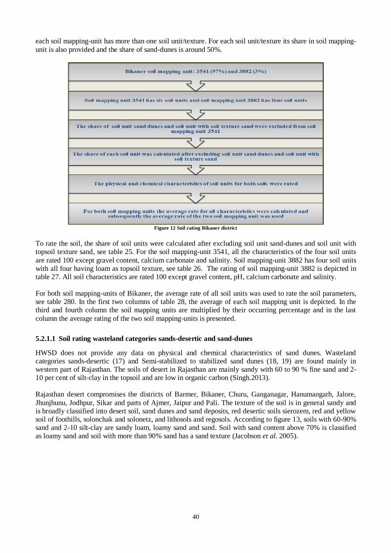
40

each soil mapping-unit has more than one soil unit/texture. For each soil unit/texture its share in soil mapping-

unit is also provided and the share of sand-dunes is around 50%.

Figure 12 Soil rating Bikaner district

To rate the soil, the share of soil units were calculated after excluding soil unit sand-dunes and soil unit with topsoil texture sand, see table 25. For the soil mapping-unit 3541, all the characteristics of the four soil units

are rated 100 except gravel content, calcium carbonate and salinity. Soil mapping-unit 3882 has four soil units with all four having loam as topsoil texture, see table 26. The rating of soil mapping-unit 3882 is depicted in table 27. All soil characteristics are rated 100 except gravel content, pH, calcium carbonate and salinity. For both soil mapping-units of Bikaner, the average rate of all soil units was used to rate the soil parameters, see table 280. In the first two columns of table 28, the average of each soil mapping unit is depicted. In the third and fourth column the soil mapping units are multiplied by their occurring percentage and in the last

column the average rating of the two soil mapping-units is presented.

5.2.1.1 Soil rating wasteland categories sands-desertic and sand-dunes

HWSD does not provide any data on physical and chemical characteristics of sand dunes. Wasteland categories sands-desertic (17) and Semi-stabilized to stabilized sand dunes (18, 19) are found mainly in western part of Rajasthan. The soils of desert in Rajasthan are mainly sandy with 60 to 90 % fine sand and 2-10 per cent of silt-clay in the topsoil and are low in organic carbon (Singh.2013). Rajasthan desert compromises the districts of Barmer, Bikaner, Churu, Ganganagar, Hanumangarh, Jalore,

Jhunjhunu, Jodhpur, Sikar and parts of Ajmer, Jaipur and Pali. The texture of the soil is in general sandy and is broadly classified into desert soil, sand dunes and sand deposits, red desertic soils sierozem, red and yellow soil of foothills, solonchak and solonetz, and lithosols and regosols. According to figure 13, soils with 60-90% sand and 2-10 silt-clay are sandy loam, loamy sand and sand. Soil with sand content above 70% is classified as loamy sand and soil with more than 90% sand has a sand texture (Jacobson et al. 2005).

41

Figure 13 Soil’s textural classes

Source: (Jacobson et al. 2005)

Table 29 contains characteristics of desert soil and the topsoil (0-20cm) has a pH of 8.4, a CaCO3 1.5% and organic carbon of 0.17%. Desert soil are the dominant soil of the area covering whole of Bikaner, Jaisalmer and Barmer districts and parts of Ganganagar, Nagaur, Churu and Jodhpur district. The topsoil of sand dunes

has a CaCO3 of 0.7% and organic carbon of 0.10%, see table 30. Looking at the composition of the desert soil and sand dunes and figure 13, it can be concluded that both desert soils and sand dunes have sand as soil texture (Dhir et al. 1978). Although the desert in Rajasthan has many different soils, as mentioned above, it was assumed that the wasteland categories sands-desertic and semi-stabilized to stabilized sand dunes belong to desert soils and sand dunes respectively (Singh. 2013; Dhir et al. 1978; Gov of Raj. 2012a). Table 29 and 30 does not provide all required data for soil rating, therefore some of other soil parameters were extracted from HWSD by using

the physical and chemical characteristics of soil unit with soil texture sand. There are four soil mapping-units (3541, 3774, 3839, and 3840), see Appendix I, which have soil unit with sand as soil texture and can be found in above mentioned districts of Rajasthan. The soil unit with soil texture sand has the same physical and chemical characteristics in all four mentioned soil mapping-units.

Figure 14 Yield estimation sand-dunes

42

The pH of the topsoil extracted from HWSD is around 6.4 and the pH given in table 29 and 30 is 8.4 for desert

soil and 8.5 for sand-dunes. However, the pH has to some extent less impact on yield of Prosopis juliflora. Soils having a pH of 5.5-6.7 and a pH of 8.1-8.7 are rated 90, therefor it does not matter whether the pH given in table 29 and 30 or pH data extracted from HWSD was used. It was assumed that the data on organic carbon used for wasteland categories land with scrub and degraded forest does not apply on wasteland categories sands-desertic and sand dunes unless its value is lower than the percentages given in table 29 and 30. Therefore, for districts where the organic carbon is lower than 0.17 and 0.1 the same organic carbon level as that for the wasteland categories land with scrub and degraded forest was used. A calcium carbonate

percentage of 0 to 20% is rated 100, it does not matter whether one use the data provided in table 29 and 30 or data extracted from HWSD since the percentage provided by both fall in the range of 0-20% . All other required physical and chemical characteristics for yield estimation were extracted from HWSD, see figure 14. In addition GIS soil fertility maps were studied to distinguish fertility of wasteland categories land with scrub, degraded forests, sands-desertic and sand dunes, though the fertility maps did not show any significant differences in organic carbon level.

5.2.2 Slope

Figure 15shows the slope map of Rajasthan and to rate the slope per district, the slope and wasteland maps of each district were studied. For districts where the wasteland categories land with dense scrub, land with open scrub and degraded forests are concentrated in one part of the district the slope of that area was used. In districts where wastelands are scattered in small patches over the area of the district, the average slope of the district was used, see figure 16. The slope of all districts and its ratings are depicted in Appendix IV.

Figure 15 Slope map of Rajasthan

Source: (India-WRIS WebGis. 2012)

As illustrated in figure 15, the slope for the state is given in four ranges, however the district-wise slope maps gives five ranges for the slope, see table 31. Per district, percentage of the occurring slope range is given; therefore prior rating the slope the average of every range was calculated and subsequently rated, see figure 16.

43

Figure 16 Slope rating steps

Table 32 shows the slope for the district of Bikaner which shows that more than 45% of the area is characterized as nearly-level. For the district of Bikaner every slope range was rated separately and the average rate of the slope ranges is 89. From figure 17 can be seen that land with dense scrub has for a large part a slope of 0-1%. However land with open scrub and degraded forest are gently sloping and steeply sloped respectively, therefore an average slope

of the district was used for Bikaner. If the wastelands were concentrated in an area with one slope range, only the slope range of that particular area would have been rated. This is a rough approach as GIS was not used to determine the slope of the studied wasteland categories.

Figure 17 Slope and wasteland map of Bikaner

44

5.2.3 Climate

The New locClim software programme and database was used in order to rate the of climate parameters depicted in table 33. The climate characteristics and rating per district and additional data on agro-climatic zones, groundwater level and constrains for plantation can be found in Appendix V.

5.3 Soil and terrain, and climate index

The soil and terrain, and climate requirements were needed to calculate the soil and terrain, and climate index. Equation 1, 2 and 3 were used to calculate soil and terrain index, climate index and climate rating. 1. IS = A x (B/100) x (C/100) x (D/100)……

2. IC = A x (B/100) x (C/100) x (D/100)……

3. RC= IC x 0.94 =16.67 -> 25.0 < IC ≤ 92; IC x 0.94 +16.67 -> 25.0 < IC ≤ 92.5; IC, -> 92.5< IC ≤ 100.0

Where IS is the soil and terrain index, IC climate index and A, B, C, D.... are the ratings of the requirements depicted in table 5 and15. Within each group of land characteristics (Chemical characteristics of soil, wetness etc.) and climate characteristics (radiation, rainfall and temperature) only the rate of most limiting factor is used to calculate the soil and terrain index, and climate index. The climate index is used to calculate the

climate rating RC, with equation 3 and subsequently land index LI is calculated with equation 4. 4. LI =RC ( IS /100)

The yield for Prosopis juliflora is calculated with equation 5 where Ymax is the maximum yield in kg/tree for Prosopis juliflora. The maximum yield used in this study, is the average weight of 11 Prosopis juliflora trees in Mombasa Kenya, see table 34. The yield for a 6 year old tree is calculated with equation 6. 5. Y(Kg/tree) = Ymax + (LI/100)

6. Yield 6 year old tree (kg/tree) = Average yield of 11 6 year old trees

In India different plantation trials have different spacing between trees. The highest density was 10000 plants per hectare on highly alkali soils. However, the table below which is taken from a study conducted in 2001 gives the recommended spacing for plantation for different purposes (Pasiecznik et al. 2001; Goel& Behl. 1998; Singh. 1998). Based on personal communication, the recommended density is 6666 trees per hectare (Suresh. 2011). The density of 1111 tress per hectare, recommended for afforestation of wastelands, was used in this study

instead of the recommended densities for energy plantation since the productivity of wasteland is very low. One of the objectives of this study was to estimate the potential of biomass from suitable wasteland categories with largest area component. However, Rajasthan has also large areas of wasteland in categories sand-dunes and sand-desertic, which are also considered suitable for plantation by MNRE. The same methodology used for yield determination of scrubland and degraded forest, was also used to determine the yield for sand dunes by assuming that sand-dunes have the characteristics of sandy soils with a plantation density of 444 plants per hectare as recommended in table 35. The estimated yields from sand dunes are presented in Chapter 7.

It was also assumed that water requirement of Prosopis juliflora would only be met by the annual rainfall. However, in some districts especially in the eastern part of Rajasthan groundwater levels are much more favourable than the western part of the state, see figure 18. This means a higher yield is possible than the estimated yield in parts of the state where the groundwater level is more favourable.

45

Figure 18 Pre-monsoon groundwater level map


As an alternative, the yield was also determined by assuming that the water requirements will be met with groundwater only. The most recent groundwater data by Central Groundwater Board was only available for 15 districts of Rajasthan (CGWB. 2011). However, India-WRIS provides data on groundwater level for the observed wells for most of the districts for the year 2003 and groundwater level map of the state of Rajasthan (India-WRIS WebGis. 2012). From the available groundwater level map of Rajasthan, district-wise maps were constructed for the district for which no maps were available. District-wise pre-monsoon groundwater level

maps are presented in Appendix VI. District-wise maps and the groundwater level of observed wells were studied and rated. The yields are somewhat lower than estimated yield where annual rainfall is assumed to provide the required water. India-WRIS provides only state-wise groundwater level map and data on observed wells is not available for all districts of Rajasthan. Therefore the estimated yield of biomass where groundwater was assumed to provide the required water was not used to estimate the economic performance of Prosopis juliflora plantation. The

estimated yields, for which the annual precipitation data extracted from New locClim was used, are more accurate than the estimated yield where groundwater level was assumed as a limiting factor since the groundwater level was rated roughly.

46

5.4 Economic performance

For the economic performance feasibility of wasteland plantation the cost of production was calculated, see equation 723.

7.

Cop = cost of production Ct = total costs Bft = total benefits r = the discount rate n= the life time of the project Yt = Yield of wood t = Year

The inflation rate in 2012 was 9.3% and it was 11.4% for the first quarter of 2013. The inflation has trended downwards since March 2013. For the sake of simplicity a constant inflation of 9% was assumed to calculate the cost of production. The lending interest rate of 11.8% used in this study is the Base Rate of the Indian Bank meant for agricultural loan (Inflation.eu. 2013; Indian-Bank. 2013; MOSPI.; Tradings-Economics.

2013). The costs of plantation establishment consist of nursery raising and planting. These costs were calculated by using data from various sources. The nursery raising cost was determined by using the model and the data provided by National Bank for Agricultural and Rural Development (NABARD), see table 37 (NABARD. 2007).

The costs of nursery-raising depicted in table 37 are for an area of 0.25 ha and 125000 seedlings, but it is not mentioned for which tree species these costs are meant. Therefore, it was adjusted for Prosopis juliflora requirements for which an area 0.4ha for 50000 seedlings was recommended (Garden-Organic.). Also, the recommended number of poly-beds, amount of seeds was adjusted for Prosopis juliflora. The costs provided by NABARD are from 2007 and were corrected for inflation of 2012, see Appendix VII. The cost of tree planting consists of land preparation, plantation, harvesting and other costs. The required

labour and material were determined by using data from plantation of 100 seedlings on one hectare land and were adjusted for 1111 seedlings, see table 38. All the required labour can be performed by unskilled labour except management and supervisory. It was assumed that for the function of management and supervisory semi-skilled and skilled labourers are needed. Labour wages used in this study depicted in table 39. Although Prosopis juliflora can survive harsh condition, watering the seedlings in the first year is recommended to increase the survival rate of the seedlings. The cost of irrigation pipelines can be very high therefore using water tanker might be a solution. The cost of water tanker used in this study is for the fresh

water meant for households. The cost of water is for the state of Maharashtra and the most accurate price that could be found for water tanker in India 24. Therefore, the actual cost of water for agriculture could be much lower than the fresh water meant for households. The estimated cost of production for biomass was compared to the price of coal in order to find out whether it is economical for coal-based power plants to replace around 10% of their cola use with biomass. It was also compared to price of crop residues like mustard husk at the power plant gate. The prices of crop residue in

various districts are from a study on biomass supply in the state of Rajasthan which are obtained from farmers and biomass based power plants.

23

The global technical and economic potential of bioenergy from salt-affected soils, Wicke et al 2011 24

http://www.hindustantimes.com/India-news/Mumbai/Rates-of-private-water-tankers-may-rise-sharply/Article1-906221.aspx

http://www.hindustantimes.com/India-news/Mumbai/Rates-of-private-water-tankers-may-rise-sharply/Article1-906221.aspx

47

5.5 Supply chains performance

The economic performance of biomass supply chains was determined for logs, chips and pellets transportation by truck. Equation 8 was used to calculate the cost of production for logs, chips and pellets.

8.

Cpre-treatment = cost of pre-treatment

To calculate the cost of pre-treatment, the data in table 40 was used and the costs were adjusted for inflation by taking an average inflation of OECD countries. The economic performance of supply chains was determined for four coal-based power plants, eight small

scale biomass-based power plants. For co-firing, it was estimated how much biomass is required if 10% of the coal would be replaced by biomass. In table 41, the capacity of power plants and the required biomass are depicted. In addition, the performance of supply chains of small scale biomass-based power plants and co-firing was compared to the performance of a non-existing large scale biomass-based power plant located in a location with the highest biomass potential and lowest production cost. There was no information available on bulk density of Prosopis juliflora and that is why, dry density of Prosopis juliflora was used to calculate the density for chopped logs. The lowest dry density given in table 42

is around 700 kg/m3. This density with the conversion factors given in table 43 and a volumetric swelling factor of 8.7 were used to calculate the bulk density of Prosopis juliflora. Equation 9 shows how the volumetric swelling factor for Prosopis juliflora was calculated. To calculate the volumetric swelling factor of Prosopis juliflora, a volumetric shrinkage of 4.7% was used (Bohra et al. 1999). 9. αv = (100xßv) / (100-ßv)

αv = Volumetric swelling factor ßv = Volumetric shrinkage factor

Volumetric swelling factor and moisture content on dry basis were used to calculate the density of logs with

30% moisture content. The conversion factor of 2 was used to estimate the density for chopped logs, see table 43. The calculated density and the densities used for pellets and chips are depicted in table 44. For pellets an average density of 700 kg/m3 was used. The cost calculations of pre-treatments for all power plants can be found in Appendix VIII-XV. The cost of transportation was calculated by using data from a study conducted by World Bank in 2005. The annual operating cost of small operators estimated by World Bank is depicted in table 45. This was used to

calculate the transportation cost of biomass for the state of Rajasthan. The costs were corrected for inflation and it was assumed that for the supply of biomass a truck with a capacity of 27 tonnes would be used. The volume of the truck was assumed to be 100 m3 and an average diesel price of Rs.49 was used for the year 2012. For the transportation of biomass from the field to the CGP a value of $0.13 was used. This value is taken from Batidzirai et al. 2013. The first transport distance, from biomass field to CGP was calculated by using the methodology described in Batidzirai et al.201225. In this methodology the transport requirements are related to the spatial distribution of

biomass in each region. The distribution over an area is assumed to be constant and the transportation of biomass takes place over a marginal distance. The distance is assumed to be equal to the radius of a circle in which the biomass is spread with the given distribution density. In order to estimate the first transport distance, the required ―delivery area‖ around the CGP is calculated by using equation 10. 10. A= P/YxCx100

A = required area for Prosopis juliflora plantation for selected power plant

25

Sustainable biomass resource availability and supply strategies for production of synfuels: Assessment of biomass production and supply from

Mozambique

48

P = Plant input capacity (in wet tonnes)

C= Coverage of energy crop (as a % of whole region) The first transport distance is then calculated by using equation 11

11. R= √A/2π Since the information on the extent of wasteland per district is available, the biomass production potential per

district was estimated. The percentage of wasteland that can be used by government and companies undertaking is 30%, therefore biomass for thermal power plants has to be supplied from more than one district. In order to calculate the first transport distance the above methodology was slightly adjusted. In table 41, the required amount of biomass per power plant is depicted. Per district it was estimated what the production potential from 30% of wasteland is. The plant input capacity in oven dry tonnes is used to calculate the area. However, if the production potential from 30% of wasteland is below the input capacity of the power plant, the production potential is used in equation 10. Subsequently, the first transportation distance is

calculated and the costs of biomass supply chains are estimated. For all power plants the biomass is assumed to be supplied from the district with the lowest cost of supply. In case not enough biomass can be supplied from a certain district, the rest of biomass is supplied from the second most economical district. The amount of biomass that needs to be supplied from the second and third district is used to calculate the cost of first transportation distance.

Figure 19 Biomass supply chain

For the distance between CGP and conversion facility to power plant, the road distance between the districts headquarters and power plants was used, see for distance between district headquarters and power plants Appendix XVI.

49

5.6 Sensitivity analysis

The costs of plantation establishment were calculated per hectare, therefore the higher the yield the lower the cost of production per GJ. Different studies on trials and plantations gave yields with significant differences,

see chapter 4.2. All the obtained data on yield for shows variation in yield, however the yield data for Rajasthan is only available for a few districts, therefore those yield were not used as lower and upper limit to illustrate the sensitivity of yield on cost of production. Instead, a range of 20% less and more biomass yield was used for sensitivity analysis to illustrate the effect of yield on production costs. Other inputs that have effect on cost of production are the labour cost, as the establishment of a plantation in India is labour intensive and discount rate. Stille states in his report that labour wages changes with labour

demand. The cost of labour is low when the demand is low and high when the demand is high. Additionally the mobility of unskilled labour is quite low; therefore the wage can differ over a distance of only 30 km (Stille et al. 2011). Sensitivity is performed for a range of 20% lower and 20% higher labour cost. According to Stille, the discount rates can be as high as 18% for commercial banks. Stille used a discount rate of 12%. The given nominal discount rate by Indian Bank is 11.75 for agricultural loan and this discount rate was used in this study. The sensitivity is performed for up to 40% higher discount rate. Sensitivity analysis was also performed for the cost of biomass transportation by varying the density of biomass logs and chips.

Regarding the yield of Prosopis juliflora, soil and terrain characteristics that have an impact on the yield are gravel content, organic carbon level and slope gradient. The lowest possible yield was calculated by rating the lowest occurring carbon level in a district, highest gravel content of a soil unit and the highest occurring slope gradient in a district. Thus, the lowest yield would be obtained if the organic carbon level is very low, the soil has high gravel content and slope gradient. To estimate the highest yield, per district the highest occurring organic carbon level, lowest gravel content and slope gradient was rated. In addition, the yield was also calculated for low carbon level, high gravel content and slope gradient by only varying the value of one of the

factors at a time.

5.7 Limitation in methodology and data

Detailed and specific data on past and current afforestation projects were not available either due to lack of proper reporting or confidentiality of information. Therefore it was not possible to use plantation data such as yield and cost of plantation from past or on-going plantation projects. The method that has been used to estimate the potential of biomass from wastelands has its limitations. The yield for every district was calculated by taking an average rating of different soil textures. It was also assumed that wasteland categories

land with dense scrub, land with open scrub and degraded forest do not have a sand texture. These three wasteland categories have different properties; still in this study it was assumed that these wasteland categories have the same chemical and physical properties. Also the slope of wasteland was rated roughly, e.g. for some districts where the wastelands are scattered over the area of the district, an average slope was used. Therefore the actual yield of a wasteland patch might be lower or higher depending on the slope of that area. A better yield result would have been obtained if GIS was used to estimate the yield of different wasteland categories.

The distances between districts headquarter and power plants were used as distance between biomass Central Gathering Point and power plant, while the actual distances from biomass field can deviate from the distances that were used. Further the cost of transport is based on the study of World Bank only as this was the only available study on road transportation in India and the logistic companies did not provide any data on transportation. Due to lack of data on cost of transportation in India, the cost of transportation from biomass field to the Central Gathering point is taken from Batidzirai et al.2013.

50

6 Data input

6.1 State and wasteland selection: Rajasthan

Rajasthan, the largest state of India with 32 districts, is located in the north-western part of the country with a geographical area of 34mha. The state is bounded in the west by Pakistan, in the north by Haryana and Punjab, in the east by Uttar Pradesh and Madhya Pradesh, and in the south by Gujarat, see figure 20.

Figure 20 District map of Rajasthan

Source: (Maps-of-India. 2009) Around 40% Rajasthan’s total geographical area is under crop land and according to data depicted in table 22, nearly 7.9mha, which is around 23% of geographical area is wasteland. This figure is lower than the 8.5mha mentioned in WAI 2011 (India-WRIS WebGis. 2013).

Table 22 Land-use statistics Rajasthan

Land-use Area in mha

% Total geographical area

Geographical area 34.2

Crop land 13.7 38.6

Fallow 6.8 19.9

Deciduous 0.9 2.6

Shrub/degraded/scrub 0.73 2.1

Grassland and grazing land 0.01 0.03

Other wasteland 7.04 20.6

Gullied/ravines 0.12 0.35

Scrub land 4.4 12.9

Water bodies 0.4 1.2

Built up land (urban & rural) 0.1 0.29


The state has been separated into western plain with two sub-physiographic zones, namely the sandy arid plain and the semi-arid transitional plain, and the central highlands with four sub-zones, the Aravalli landscape, the

eastern Rajasthan upland, the Pathar and Bundelkhand uplands, and the Malwa plateau. The climate of Rajasthan ranges from semi-arid to arid on the west of Aravallis and semi-arid to sub-humid on the east of Aravallis. The mean annual rainfall in the western part of Rajasthan varies from less than 100 to 400mm and it

51

ranges between 557mm and 1000mm in the east of the state, see figure 21. The mean annual temperature

varies between 24°C and 27°C. In the western part, the average temperature in months of May and June is around 40° -43° and mean winter temperature drops to 13°C during December to January. The west part of the state, including the Thar Desert, is very dry and arid. In the south-western part of the state, the land is wetter, hilly, and more fertile (Trivedi. 2010; MOEF. 2011b).

Figure 21: Annual rainfall Rajasthan

Source: (RPCB26.)

Among the 32 districts, Jaisalmer is highly degraded with 2.5mha, followed by Bikaner and Barmer with

0.85mha and 0.5mha respectively. Figure 22 illustrates district-wise area of total wasteland and percentage of total geographical area as wasteland. According to MNRE, a small area and high percentage means that wasteland is less scattered over the area of district and can be used for large scale plantation. This means that the wastelands in districts of Barmer, Bikaner and Jaisalmer are scattered and cannot be used for large scale plantation.

Figure 22 District-wise wasteland area and percentage of total geographical area

Out of 23 wasteland categories, only 19 categories can be found in the state of Rajasthan, see figure 23 (MORD. 2011). The total areas of wasteland categories land with scrub, land without scrub and degraded

forest is around 8.4mha out of which nearly 5mha can be found in the state of Rajasthan.

26

Rajasthan State Pollution Control Board

52

Figure 23: Wasteland map of Rajasthan


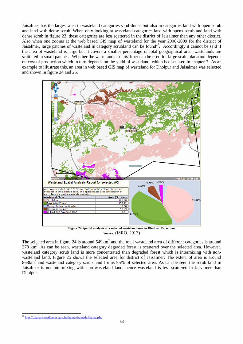
53

Jaisalmer has the largest area in wasteland categories sand-dunes but also in categories land with open scrub

and land with dense scrub. When only looking at wasteland categories land with opens scrub and land with dense scrub in figure 23, these categories are less scattered in the district of Jaisalmer than any other district. Also when one zooms at the web based GIS map of wasteland for the year 2008-2009 for the district of Jaisalmer, large patches of wasteland in category scrubland can be found27. Accordingly it cannot be said if the area of wasteland is large but it covers a smaller percentage of total geographical area, wastelands are scattered in small patches. Whether the wastelands in Jaisalmer can be used for large scale planation depends on cost of production which in turn depends on the yield of wasteland, which is discussed in chapter 7. As an

example to illustrate this, an area in web based GIS map of wasteland for Dholpur and Jaisalmer was selected and shown in figure 24 and 25.

Figure 24 Spatial analysis of a selected wasteland area in Dholpur Rajasthan

Source: (ISRO. 2013)

The selected area in figure 24 is around 549km2 and the total wasteland area of different categories is around 278 km2. As can be seen, wasteland category degraded forest is scattered over the selected area. However, wasteland category scrub land is more concentrated than degraded forest which is intermixing with non-wasteland land. Figure 25 shows the selected area for district of Jaisalmer. The extent of area is around 868km2 and wasteland category scrub land forms 85% of selected area. As can be seen the scrub land in Jaisalmer is not intermixing with non-wasteland land, hence wasteland is less scattered in Jaisalmer than Dholpur.

27

http://bhuvan-noeda.nrsc.gov.in/theme/thematic/theme.php

http://bhuvan-noeda.nrsc.gov.in/theme/thematic/theme.php

54

Figure 25 Spatial analysis of a selected wasteland area in Jaisalmer Rajasthan

Source: (ISRO. 2013)

The wasteland map of Rajasthan shows that sandy wasteland categories can be found in western part of the state while degraded forests are more in the eastern part of the state the largest area in wasteland category degraded forest can be found in the district of Udaipur, Baran, Karuali and Chittaurgarh. This can also be seen from figure 23 and it can also be seen that for example in district of Dungarpur and Kota degraded forests are less scattered compared to wasteland category land with scrub. Wasteland categories with large area in the state of Rajasthan are wasteland categories sands-desertic and sand-dunes covering 34% of the total geographical area of Rajasthan. Jaisalmer and Bikaner are the districts with largest area in the last mentioned categories where the annual rainfall is also quite low compared to the eastern part of the state.

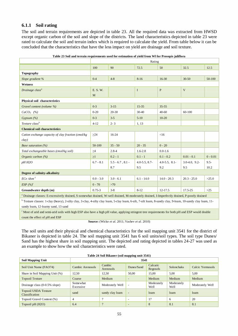
55

6.1.1 Soil rating

The soil and terrain requirements are depicted in table 23. All the required data was extracted from HWSD except organic carbon of the soil and slope of the districts. The land characteristics depicted in table 23 were rated to calculate the soil and terrain index which is required to calculate the yield. From table below it can be

concluded that the characteristics that have the less impact on yield are drainage and soil texture.

Table 23 Soil and terrain requirements used for estimation of yield from Wl for Prosopis juliflora

Rating

100 90 72.5 50 32.5 12.5

Topography

Slope gradient % 0-4 4-8 8-16 16-30 30-50 50-100

Wetness

Drainage classa E. S. W.

M

I P V

Physical soil characteristics

Gravel content (volume %) 0-3 3-15 15-35 35-55

CaCO3 (%) 0-20 20-30 30-40 40-60 60-100

Gypsum (%) 0-3 3-5 5-10 10-20

Texture classb 4-12 2- 3 1, 13

Chemical soil characteristics

Cation exchange capacity of clay fraction (cmol/kg

clay)

≥24 16-24 <16

Base saturation (%) 50-100 35 - 50 20 - 35 0 - 20

Total exchangeable bases (cmol/kg soil) ≥4 2.8-4 1.6-2.8 0.0-1.6

Organic carbon (%) ≥1 0.2 - 1 0.1 - 1 0.1 - 0.2 0.01 - 0.1 0 - 0.01

pH H2O 6.7 - 8.1 5.5 - 6.7 , 8.1 -

8.7

4.0-5.5, 8.7-

9.5

4.0-5.5, 8.1-

9.2

3.0-4.0, 9.2-

9.5

9.5-

10.2

Degree of salinity-alkalinity

ECe /dsm-1 0.0 - 3.0 3.0 - 6.1 6.1 - 14.0 14.0 - 20.3 20.3 - 25.0 >25.0

ESP (%)c 0 - 70 >70

Groundwater depth (m) 0.75-3 3-8 8-12 12-17.5 17.5-25 >25

a Drainage classes: E-excessively drained, S-somewhat drained, W-well drained, M-moderately drained, I-Imperfectly drained, P-poorly drained

b Texture classes: 1-clay (heavy), 2-silty clay, 3-clay, 4-silty clay loam, 5-clay loam, 6-silt, 7-silt loam, 8-sandy clay, 9-loam, 10-sandy clay loam, 11-

sandy loam, 12-loamy sand, 13 sand

c Most of arid and semi-arid soils with high ESP also have a high pH value, applying stringent tree requirements for both pH and ESP would double

count the effect of pH and ESP

Source: (Wicke et al. 2011; Vashev et al. 2010)

The soil units and their physical and chemical characteristics for the soil mapping unit 3541 for the district of Bikaner is depicted in table 24. The soil mapping unit 3541 has 6 soil units/soil types. The soil type Dunes/ Sand has the highest share in soil mapping unit. The depicted and rating depicted in tables 24-27 was used as

an example to show how the soil characteristics were rated.

Table 24 Soil Bikaner (soil mapping unit 3541)

Soil Mapping Unit 3541

Soil Unit Name (FAO74) Cambic Arenosols Cambic

Arenosols Dunes/Sand

Calcaric

Regosols Solonchaks Calcic Yermosols

Share in Soil Mapping Unit (%) 12,50 12,50 50,00 15,00 5,00 5,00

Topsoil Texture Coarse Medium - Medium Medium Medium

Drainage class (0-0.5% slope) Somewhat

Excessive Moderately Well -

Moderately

Well

Moderately

Well Moderately Well

Topsoil USDA Texture

Classification sand sandy clay loam - loam loam loam

Topsoil Gravel Content (%) 4 7 - 17 6 20

Topsoil pH (H2O) 6.4 7 - 8 8.1 8.1

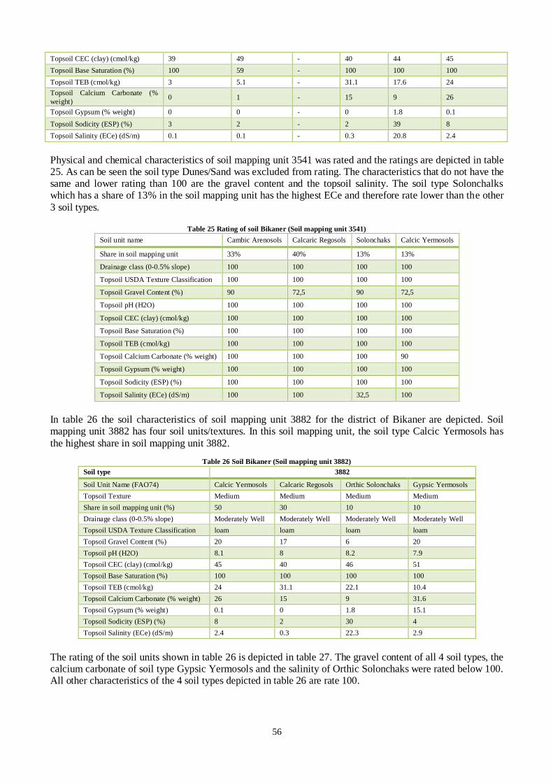
56

Topsoil CEC (clay) (cmol/kg) 39 49 - 40 44 45

Topsoil Base Saturation (%) 100 59 - 100 100 100

Topsoil TEB (cmol/kg) 3 5.1 - 31.1 17.6 24

Topsoil Calcium Carbonate (%

weight) 0 1 - 15 9 26

Topsoil Gypsum (% weight) 0 0 - 0 1.8 0.1

Topsoil Sodicity (ESP) (%) 3 2 - 2 39 8

Topsoil Salinity (ECe) (dS/m) 0.1 0.1 - 0.3 20.8 2.4

Physical and chemical characteristics of soil mapping unit 3541 was rated and the ratings are depicted in table 25. As can be seen the soil type Dunes/Sand was excluded from rating. The characteristics that do not have the same and lower rating than 100 are the gravel content and the topsoil salinity. The soil type Solonchalks which has a share of 13% in the soil mapping unit has the highest ECe and therefore rate lower than the other

3 soil types.

Table 25 Rating of soil Bikaner (Soil mapping unit 3541)

Soil unit name Cambic Arenosols Calcaric Regosols Solonchaks Calcic Yermosols

Share in soil mapping unit 33% 40% 13% 13%

Drainage class (0-0.5% slope) 100 100 100 100

Topsoil USDA Texture Classification 100 100 100 100

Topsoil Gravel Content (%) 90 72,5 90 72,5

Topsoil pH (H2O) 100 100 100 100

Topsoil CEC (clay) (cmol/kg) 100 100 100 100

Topsoil Base Saturation (%) 100 100 100 100

Topsoil TEB (cmol/kg) 100 100 100 100

Topsoil Calcium Carbonate (% weight) 100 100 100 90

Topsoil Gypsum (% weight) 100 100 100 100

Topsoil Sodicity (ESP) (%) 100 100 100 100

Topsoil Salinity (ECe) (dS/m) 100 100 32,5 100

In table 26 the soil characteristics of soil mapping unit 3882 for the district of Bikaner are depicted. Soil mapping unit 3882 has four soil units/textures. In this soil mapping unit, the soil type Calcic Yermosols has

the highest share in soil mapping unit 3882.

Table 26 Soil Bikaner (Soil mapping unit 3882)

Soil type 3882

Soil Unit Name (FAO74) Calcic Yermosols Calcaric Regosols Orthic Solonchaks Gypsic Yermosols

Topsoil Texture Medium Medium Medium Medium

Share in soil mapping unit (%) 50 30 10 10

Drainage class (0-0.5% slope) Moderately Well Moderately Well Moderately Well Moderately Well

Topsoil USDA Texture Classification loam loam loam loam

Topsoil Gravel Content (%) 20 17 6 20

Topsoil pH (H2O) 8.1 8 8.2 7.9



Topsoil TEB (cmol/kg) 24 31.1 22.1 10.4

Topsoil Calcium Carbonate (% weight) 26 15 9 31.6

Topsoil Gypsum (% weight) 0.1 0 1.8 15.1


Topsoil Salinity (ECe) (dS/m) 2.4 0.3 22.3 2.9

The rating of the soil units shown in table 26 is depicted in table 27. The gravel content of all 4 soil types, the calcium carbonate of soil type Gypsic Yermosols and the salinity of Orthic Solonchaks were rated below 100. All other characteristics of the 4 soil types depicted in table 26 are rate 100.

57

Table 27 Rating soil Bikaner (soil mapping unit 3882)

Soil mapping unit 3882


Share in soil mapping unit 50% 30% 10% 10%

Drainage class (0-0.5% slope) 100 100 100 100

Topsoil USDA Texture Classification 100 100 100 100

Topsoil Gravel Content (%) 72,5 72,5 90 72,5

Topsoil pH (H2O) 100 100 90 100



Topsoil TEB (cmol/kg) 100 100 100 100

Topsoil Calcium Carbonate (% weight) 90 100 100 72,5



Topsoil Salinity (ECe) (dS/m) 100 100 32,5 100

Table 28 shows the average rate of the soil mapping units and the average of soil rating for the district of Bikaner. Table 28 shows that the gravel content and salinity have the lowest rating compared to other characteristics.

Table 28 Average rating of soil mapping units

Soil characteristics Average 3541 Average 3882 3541 (97%) 3882(30%) Average of 3541and 3882

Drainage class (0-0.5% slope) 100 100 97 3 100

Topsoil USDA Texture Classification 100 100 97 3 100

Topsoil Gravel Content (%) 81 74 78 3 80

Topsoil pH (H2O) 100 99 97 3 100

Topsoil CEC (clay) (cmol/kg) 100 100 97 3 100

Topsoil Base Saturation (%) 100 100 97 3 100

Topsoil TEB (cmol/kg) 100 100 97 3 100

Topsoil Calcium Carbonate (% weight) 99 92 95 3 98

Topsoil Gypsum (% weight) 100 95 97 3 100

Topsoil Sodicity (ESP) (%) 100 100 97 3 100

Topsoil Salinity (ECe) (dS/m) 91 93 88 3 91

The mechanical composition and chemical characteristics of desert soil are depicted in table 29. Together with data extracted from HWSD, the data from table 29 and 30 was used to rate the physical and chemical characteristics of wasteland categories sand-desertic and sand dunes.

Table 29 Mechanical composition and chemical characteristics of desert soil

Depth (cm) Coarse sand Fine sand Silt Clay CaCO3 pH Organic C

0-20 21.3 70.7 2.6 5.4 1.5 8.4 0.17

20-60 15.0 70.3 6.3 8.4 7.3 8.6

60-90 14.2 71.1 8.4 6.3 9.13 8.5

90-120 18.8 70.2 7.3 3.7 7.45 8.5

In table 30 the mechanical and chemical composition of sand dunes are depicted. According to data depicted in table 30, the wasteland category sand dunes have a sandy soil type. Based on the data depicted in table 29 and 30 and figure 13 which shows the soil’s textural classes, the characteristics of sandy soil types were extracted from HWSD to rate wasteland categories sand-desrtic and sand dunes.

Table 30 mechanical composition and chemical characteristics of sand dunes

Depth (cm) Coarse sand Fine sand Silt Clay CaCO3 pH Organic C

0-30 22.4 70.5 1.4 4.7 0.7 8.5 0.10

30-60 11.4 81.1 1.1 5.0 0.6 8.5

60-90 14.7 78.1 1.1 4.8 0.6 8.5

90-120 12.5 82.7 1.0 3.9 0.5 8.5

120-150 14.0 81.0 0.4 2.5 0.6 8.5

150-180 14.2 78.8 1.5 3.3 0.8 8.5

180-210 13.8 80.3 2.0 2.9 0.8 8.5

58

Table 31 contains slope ranges for the state of Rajasthan. It also contains the average of every range and their ratings. A slope gradient of 0-1 is considered nearly level and the average slope gradient of nearly level is 0.5% which is rated 100. A slope of 1-3 is described as very gently sloping and is also rated 100. Moderately sloping and steeply sloping is rated 72.5 and 32.5 respectively.

Table 31 Slope rating

Description Slope (%) Average slope (%) Rating

Nearly level (0-1%) 0-1 0,5 100

Very gently sloping (1-3%) 1-3 2 100

Gently sloping (3-8%) 3-8 5,5 90

Moderately sloping (8-15%) 8-15 11,5 72.5

Steeply sloped (>30%) >30 >30 32,5

The slope and the related relative area and their ratings for the district of Bikaner are depicted in table 32.

Table 32 shows that around 45% area of Bikaner has slope between 0-1% which is described as nearly level. As shown in table 31, the average nearly level is 0.5% and is rated 100. Since 45.5% of the area is nearly level the weighted rate is 45.5. The average slope rate for district of Bikaner is 89.

Table 32 Slope rating Bikaner

Description Area (%) Rating Weighted rate

Nearly level (0-1%) 45,5 100 45,5

Very gently sloping (1-3%) 0,0 - -

Gently sloping (3-8%) 30,0 90 27

Moderately sloping (8-15%) 21,9 72.5 15,9

Steeply sloped (>30%) 2,5 32,5 0,8

Average - - 89

59

6.1.2 Climate rating

Table 33 was used to rate the climate parameter and the climate data was extracted from New locClim. The table below shows that data on annual perception, mean maximum temperature, mean annual temperature, mean minimum temperature and fraction of sunshine hours are needed.

Table 33 Climate requirements Prosopis juliflora

Rating

100 90 72.5 50 32.5 12.5 0

Rainfall ≥1200 750-1200 550-750 300-550 100-300 0-100

Annual perception 0-6 6-7 7-8 8-10 10-11 11-12

length of dry season/months

Temperature 20-30 30-34 34-42 42-50 50-55 >55

Mean max temp 20-30 (30-35) (18-20) (35-38) (16-18) (38-42) (14-16) (42-45) (12-14) >45 <12

Mean annual temp 20-25 (16-20) (25-35) 12-16 8-12 5-8 <5

Mean min temp

Radiation

Fraction of sunshine hours 0.7-1.0 0.5-0.7 0.0-0.5

6.1.3 Climate rating and yield calculation

Yield in kg/tree of 6 year old trees in Mombasa Kenya are depicted in table 34. The average yield of large branches and stem was used as Ymax to estimate the yield of biomass from wastelands.

Table 34 Oven dry weight of 6 years old Prosopis juliflora

No Small branches Large branches Stem Total

1 0,8 0,0 2,8 3,7

2 3,5 0,0 4,4 7,9

3 2,8 1,8 8,2 12,7

4 13,5 5,6 23,1 42,1

5 12,3 8,1 40,5 61,0

6 27,2 20,4 63,4 111,1

7 15,1 20,1 60,2 95,4

8 57,6 45,9 146,8 250,3

9 45,2 59,9 113,9 218,9

10 46,0 67,9 128,4 242,2

11 44,2 51,7 276,5 372,3

Source: (Maghembe et al. 1983)

The recommended densities for Prosopis juliflora for different plantation types and purposes are depicted in table 35. For afforestation of degraded land a density of 1111 plants per hectare is recommended. For energy plantation, with the main purpose fuel-wood production, densities of 3333 and 2500 plants per hectare is recommended.

Table 35 Recommended plantation densities for various types of Prosopis juliflora plantation

Purpose Spacing

Plantation type Main Secondary Row to row Plant to plant Density

Afforestation degraded land Land/soil conservation Fuel-wood production 3 3 1111

Sand dune stabilization Land/soil conservation Fuel-wood production 5 5 400

Energy plantation Fuel-wood production Charcoal/pod 3/2 / 2 3333/2500

Fodder production Pod production Fuel-wood/seed 6 /5 4 /5 416/400

Timber production Timber Pods for fodder and seeds 10 5 200

Seed orchard Improved seed pods for fodder 6 6 278

Hedge row Live fences Shelter, erosion control 0.3-0.5 0.5 n/a

Agroforestry and agri-

silviculture Fuel and fodder

Production of associated

crops 10 10 100

Silvo-pastoral Fuel and fodder Production of

grasses/animals 10 5 200

60

Road and river sides, field

boundaries

Aesthetic value, wind break, soil

conservation Pods for fodder Single row 3_5 n/a

Shelterbelts Soil/moisture conservation, reducing

wind speed

Pods for fodder, shades for

livestock 3 3 n/a


6.2 Economic performance

The nominal interest rate used for cost of production calculation is depicted in table 35.

Table 36 Discount rate

Discount rate 11.75%

Inflation 9%

Source: (Inflation.eu. 2013; Indian Bank. 2013; MOSPI.; Tradings Economics. 2013)

The cost of forest nursery depicted in table 19 was adjusted to calculate the cost of nursery-raising for 50000 Prosopis juliflora seedlings using an area of 0.4ha.

Table 37 Forest nursery

Particulars of works Unit Cost. (Rs.)

Fixed Cost

Site Preparation 8 MD 400

Fencing with barbed wire for 150 RMT Rs.30/RMT 4500

Preparation of compost pit, nursery path 10 MD 500

Maintenance of irrigation source LS 2000

5 HP Diesel Pump set LS 25000

Cost of pipeline for irrigation (100 m.) Rs.15/RMT 1500

Cost of implements for nursery operations LS 2500

Cost of Water Tank LS 5000

Preparation of Polybeds (120) 100 MD 5000

Cost of Net for providing shade and installation LS 30000

Subtotal 76400

Contingency 5% 3820

Total 80220

Recurring Cost

Particulars of works Unit Cost. (Rs.)

Rent for land 0.25 ha. Rs.2500/yr 2500

Preparation of Seed beds (10) 10MD 500

Cost of seeds LS 5000

Cost of Polybags (400 Polybags/kg) Rs.40/kg 12000

Cost of Pot mixture including loading, unloading ( 2 kg/bag) Rs.120/MT 30000

Cost of fertilizer (10 gm./polybag required) Rs.10/kg 12000

Cost of chemicals for plant protection LS 2500

Cost of diesel and lubricants for pump sets (1.5 hrs. for 100 days) 1 L. /hr. @ Rs.22/lL 3300

Cost of thatching material LS 1000

Cost of sowing on seed beds 10 MD 500

Cost of weeding and hoeing 50 MD 2500

Cost of picking up from germi beds 50 MD 2500

Filling up of polybags (200 Polybags /MD) 625 MD 31250

Shifting of polybags 50 MD 2500

Cost of labour for irrigation 100 MD 5000

Cost of fertilizer application 25 MD 1250

Cost of application of insecticides 25 MD 1250

Maintenance of paths 10 MD 500

Maintenance of pump set LS 2500

Watch and ward Rs.1000/month 12000

Subtotal 130550

Cost of supervision 5% 6527

61

Total 137077

Grand Total 217297

Source: (NABARD. 2007)

The calculated costs of plantation are presented in table 38. It was assumed that biomass is harvested every 2 year.

Table 38 Cost of plantation

Required Unit Price Unit Y1 Y2 Y3 Y4 Y Y6 Total Unit

Land preparation

Fencing area with strand

barbed wire (m) 300 RMT/1ha 48 Rs./RMT 14414 0 0 0 0 0 14414 Rs.

Building of micro-

windbreaks 0 0 0 0 0 0 0 0 Rs.

Site preparation,

alignment ploughing

and staking

1602 Rs./ha 1602 0 0 0 0 0 1602

Remarking of the area 3 MD 147 Rs./MD 441 0 0 0 0 0 441 Rs.

Opening of lanes 3 MD 147 Rs./MD 441 0 0 0 0 0 441 Rs.

Land preparation cost/ha

16897 Rs./ha

Planting cost

Placement of marks for

planting 33 MD 147 Rs./MD 4900 0 0 0 0 0 4900 Rs.

Digging pits and

backfilling with the soil 1111 Pits/ha 6 Rs./pit 7117 0 0 0 0 0 7117 Rs.

Seedling allotment 11 MD 147 Rs./MD 1633 0 0 0 0 0 1633 Rs.

Fertilizer 25 gms/plant 13 Rs/kg 356 356 356 0 0 0 1068 Rs.

Farm yard manure (2-

3kg/pit) 3 tonne 354 Rs./ton 1063 0 0 0 0 0 1063 Rs.

Water tanker (10000

ltr/tanker) 6 tanker 1700 Rs./tanker 10200 0 0 0 0 0 10200 Rs.

planting cost /tree 23 Rs./tree

Harvesting cost

Manual28

Labour required for

harvesting 1,88 MD/tonne 147 Rs./MD 0 276 0

27

6 0

27

6 276

Rs./ton

ne

Treatment

Hoeing (for 3 years) 12 MD/yr 147 Rs./MD 1764 1764 1764 0 0 0 5292 Rs./ha

Manual harvesting

machinery cost

Harvesting tools - - 51 Rs./tonne 51 Rs./ton

ne

Other costs

Supervisory staff 1 MD/50MD 167 Rs./MD 334 167 0 16

7 0

16

7 835

Contingency 10% annual cost

Managerial staff 3 MD 217 Rs./MD 651 651 Rs./ha

Source: (Pasiecznik et al. 2001; Wicke et al. 2011; DFID et al. ; The Indian Express. 2011; Seshadri et al. 1978)

The minimum labour wages for unskilled, semi-skilled, skilled and highly skilled used in this study are presented in table 39. The depicted labour wages in table 39 are for the state of Rajasthan for the year 2012.

Table 39 Labour wages

Labour Minimum wages in Rajasthan 2012 (Rs./manday)

Unskilled Semi-skilled Skilled Highly skilled

147 157 167 217

Source: (Gov of Raj. 2012b)

28

The cost for manual harvesting is taken from Wicke et. Al 2011

62

6.3 Supply chains performance

The data in table 40 was used to estimate the cost of sizing, drying and pelletizing for 12 power plants under the study. The matter loss during sizing and drying due to the action was assumed to be zero.

Table 40 Data for estimating cost of pre-treatment

Sizing Drying Densification

Roll crusher Hammermill Rotary drum Pellet press

Base scale (tonne/h) 10 50 100 6

Base capital (M$) 0,14 0,37 5 0,12

Scale factor R 0,7 0,7 0,7 0,61

Load factor (%) 90 90 100 90

O&M (%) 20 20 3 197

Lifetime 15 15 15 10

Energy-e (kWh/tonne) 8,22 3,5 20 28

Energy-h 2,5GJ/twe

Form Chips Chips Chips Pellets

Average particle size (mm) 3000 to 30 30 to 10 30 10

Bulk density (kg/m3 bulk)

All matter loss/action (%) 2 2 1

Moisture content (%) 7 8

Source: (Hamelinck et al. 2005)

In table 41 the capacity, annual fuel requirement and the amount of biomass delivered for the coal based thermal power plants and biomass based power plants under study are depicted. As can be seen, there are eight biomass-based power plants, however only four of them are actually operating.

Table 41 Existing power plants in Rajasthan

Power plants Fuel Capacity

(MW)

Annual fuel

Requirement

(PJ)

Cola replaced

by biomass

(PJ)

Biomass input

(odt/year)

Chhabra Thermal Power Station (Baran) Coal 500 36.6 3.7 203389

Kota Thermal Power Station (Kota) Coal 1240 113.5 11.4 630720

Suratgarh Super Thermal Power Station

(Ganganagar) Coal 1500 134 13.4 744600

Kalisindh Thermal Power Stationn (Jhalawar) Coal 1200 94 9.4 522667

S M Environmental Technologies (P) Ltd. (Baran) Biomass 8 0.8 - 44851

Kalpataru Power Transmission Ltd. (Ganganagar) Biomass 7.8 0.8 - 43730

Amrit Environmental Technologies (Jaipur) Biomass 8 0.8 - 44851

Transtech Green Power Pvt. Ltd. (Jalore) Biomass 12 1.2 - 67277

Surya Chambal Power Ltd (Kota) Biomass 7.5 0.76 - 42048

Sathyam Power Pvt. Ltd. (Nagaur) Biomass 10 1 - 56064

Sambhav Energy Ltd. (Sirohi) Biomass 20 2 - 112128

Kalpataru Power Transmission Ltd (Tonk ) Biomass 8 0.8 - 44851

Source: (RRECL. 2013; RVUN. 2013) In table 42 the moisture content, green density and dry density of Prosopis juliflora is presented. This was

used to calculate the bulk density for Prosopis juliflora logs.

63

Table 42 Properties of Prosopis juliflora in different regions

Location Moisture content % Specific gravity Density green (kg/m3) Density dry (kg/m3) Source

Brazil 29.8 - - 910 Lima 1994

Brazil 31.1-40.8 - 745-934 - Riegelhaupt et al 1990

Brazil 33.2 - 1126 - IPA 1989

Sudan 38.7 0.77 1151 708 El Fadl 1997

S. Arabia - 0.55-0.66 - Abohassan et al 1988

Pakistan - 0.57-1.07 - - Khan et al 1986

India 42.0 0.74-0.76 1052 848 Shukla et al 1990

India 43.2-46.3 0.78-0.85 1123-1251 - Sekhar and Rawat 1960

India - 0.83-0.86 - - Kazmi and Singh 1992

India 46.3 0.85 1249 - Sanyal and Saxena 1980

India 45.0 - - 730 Pandey et al 1990

India - - - 800-890 Goel and Behl 1992


The conversion factors required for calculating bulk density of chopped logs and wood chips are depicted in table 43. The conversion factor 1.2 was used to calculate the density of stacked logs from round wood. For Prosopis juliflora chips and pellets a density of 240kg/m3and 700kg/m3 was used to estimate the cost of transportation.

Table 43 Conversion factors

Assortments Roundwood

m3

One-meter logs woods

stacked m3 Chopped logs woods m3 Wood chips bulk m3

stacked bulked fine (G30) Medium (G50)

1 m3 roundwood 1 1,4 1,2 2 2,5 3

1 stacked m3 one-meter log

woods 0,7 1 0,8 1,4 1,75 2,1

1 stacked m3 chopped log woods 0,85 1,2 1 1,7

1 bulk m3 chopped log woods 0,5 0,7 0,6 1

1 bulk m3forest chips fine (G30) 0,4 0,55 1 1,2

1 bulk m3 chips medium (G50) 0,33 0,5 0,8 1

Source: (Francescato& Krajnc. 2009; KRAJNC. )

In table 44 density of Prosopis juliflora, lower heating value per cubic metre and tonne are depicted. These values were used to calculate the cost of transportation in $/GJ/km.

Table 44 Density of Prosopis juliflora

Moisture content Density kg/m3 GJ/t

Chopped logs mc 30% 460 12,6

Chips mc 30% 240 12,6

Pellets mc 10% 700 16,2

64

6.4 Freight transport and road connectivity

A power plant using biomass as feedstock requires steady and reliable supply of biomass from land to the power plant, thus transport is a key issue throughout the supply chain of biomass. The Indian railway carries around two million tonnes of freight a day and has a leading role in carrying cargo across India vast territory, yet most of its major corridors have capacity constraints. In contrast, roads are the dominant mode of

transportation and carry 65 per cent of India’s freight. The cost of freight transportation by rail is higher than in most other countries because freight tariffs are kept high in order to subsidize the passenger traffic. On the other hand, the presence of large number of small truck operators in road transport industry has led to a fragmented industry causing the rates of freight transport to decrease significantly (Bansal et al. 2005; MORTH. 2011). The road transport industry in India is highly competitive with lowest freight rates in the world, but at the

same time with poor service quality, low reliability and transit times. According to a World Bank on road transport in India, the cost of transportation varies little from the freight rates. The low freight rates have led to low profit and even to losses. Despite the low rates for freight transport the cost of transportation can stil l be high for light-loading freight as the volume of the trucks in India is around 30-40m3 (Bansal et al. 2005; Mehta. 2012). According to a study on economics of trucking industry, there are no statistics available on volume and nature of transported goods by roads except broad estimation of overall transported volume per annum (MORTH.

2011). Further, the available freight rates are usually for a 9 tonne truck between major cities. Freight rates are not available per tonne per km and also no distinguish can be made between different goods that has to be transported.

6.4.1 Road connectivity and road density of Rajasthan

The density of highway network of India was around 0.66km per km2 similar to the density of United States and much larger than that of Brazil and China which is only 0.16 and 0.20 km per km2 respectively. However

around 40 per cent of villages in India lacked all weather roads, especially in northern and north-eastern states of the country in the year 2000. Further the roads in India have a poor quality and are congested and the maintenance of it remains unfunded (Bansal et al. 2005). Rajasthan has around eleven per cent of total geographical area of the country but it has only six per cent of the total road length as per 2011. According to Rajasthan’s State Development Report for the year 2006, the road density was around 0.338km/km2, far below the national average of 0.66km/km2. However, the most

recent data shows that the road density have increased for Rajasthan. As on 2012, the road density is said to be around 1.25km per km2.The data on village connectivity shows that villages with a population group of 1000 or above have almost a connectivity of 100% and the village with a population group of 500 to 1000 have slightly lower connectivity. On the other hand, smaller villages with a population group of below 500 people have a very low connectivity; see Appendix XVI (Gov of Raj. 2013d; MOSPI. 2013; PC. 2006a; Gov of Raj. 2013c).

When looking at connectivity of all villages per district, Jalore, Jhunjhunu and Jodhpur are the districts with relatively highest connectivity and Baran, Chittaurgarh and Hanumangarh are the districts with lowest connectivity. However when looking at the number of villages with a population group of below 500, Ganganagar, Hanumangarh and Udaipur have the highest number of unconnected villages while Sirohi and Karuali are the districts with highest connectivity (Gov of Raj. 2013d). The wasteland map of Rajasthan in figure 23 shows that the western part of Bikaner and Jaisalmer district is not connected to main roads and railway. However this could be due to low population density of Bikaner and

Jaisalmer with 78 and 17 person per km2 which is much lower than the state average of 201 persons per km2. Also compared to districts with much smaller area like Bhilwara, Jaisalmer has only about 600 villages, while the number of villages in Bhilwara is around 1700 (Gov of Raj. 2011). This means that large parts of Jaisalmer, like the western part where large areas of sand dunes can be found, is not well connected by road.

65

In 2005, the World Bank conducted a study on road transportation in India. This was the only study on road

transportation providing insight on truck transportation and operating cost of truck operators in India. The annual operating costs of small truck operators presented in table 45 were used to calculate the cost of transportation for selected supply chains.

Table 45 Annual operating costs of small operators estimated by World Bank (Rs)

Type of truck

5 tonne 9 tonne 16 tonne 27 tonne

Fuel 150000 356000 492300 711100

Lubricants 9000 24000 28000 40000

Tyres 37800 67200 105600 182400

Spares 9000 24000 28000 40000

Crew 67500 91100 112500 168600

Maintenance 9000 24000 28000 40000

Wayside labour/repairs 11250 40000 60000 80000

Overheads expenses

-Staff/Administration 0 0 0 0

-Tax 27690 47690 49330 54910

-Interest 16800 22400 29400 63000

-Depreciation 60000 80000 105000 225000

-Other 27900 54300 72700 112400

-Profit 15900 31100 41500 64200

Total overheads 148290 235490 297930 519510

Total cost 441840 861790 1152330 1781610

Annual Utilization (km) 45000 80000 80000 80000

Cost per truck km 9.8 10.8 14.4 22.3

Cost per ton km of capacity 1.96 1.20 0.90 0.82

Source: (Bansal et al. 2005)

66

7 Results and Discussion

7.1 Biomass potential

The potential of biomass from wastelands has been calculated for all districts and different wasteland categories. This calculation covers land with open scrub, land with dense scrub and land under-utilised/degraded forests. The total area of wasteland in Rajasthan is around 8.5mha out of which 4.74mha is under wasteland categories land with scrub, land without scrub and degraded forests. The area under wasteland categories sands-desertic and sand dunes is approximately 2.7mha, see table 46.

Table 46 District-wise area of wasteland categories 3, 4, 11 and 17-19

Area wasteland categories (kha)

3 4 11 17 18 19 Total

Ajmer 56 108 20 1 0 0 185

Alwar 50 5 10 0 0 0 65

Barmer 62 72 11 16 131 139 431

Banswara 17 18 63 0 0 0 98

Baran 29 17 116 0 0 0 162

Bharatpur 28 13 4 0 0 0 45

Bhilwara 141 81 35 0 0 0 257

Bikaner 13 40 7 95 101 530 787

Bundi 26 8 72 0 0 0 106

Chittaurgarh 77 39 90 0 0 0 206

Churu 15 24 0 1 0 3 44

Dausa 19 6 6 0 0 0 32

Dholpur 34 10 29 0 0 0 73

Dungarpur 40 55 31 0 0 0 126

Ganganagar 8 8 0 17 0 93 125

Hanumangarh 2 4 2 10 0 12 31

Jaipur 22 82 38 1 0 0 142

Jaisalmer 775 357 11 55 682 490 2369

Jalore 28 9 15 24 2 11 89

Jhalawar 78 30 53 0 0 0 161

Jhunjhunu 7 29 17 1 0 0 54

Jodhpur 36 91 6 100 12 138 383

Karauli 32 9 110 0 0 0 150

Kota 40 10 53 0 0 0 103

Nagaur 29 48 13 9 0 9 107

Pali 120 41 19 0 0 0 181

Rajsamand 78 67 3 0 0 0 148

Sikar 11 31 29 4 0 0 76

Sirohi 52 41 50 3 0 1 148

Sawai madhopur 17 13 34 1 0 0 64

Tonk 32 27 10 0 0 0 70

Udaipur 136 143 138 0 0 0 417

Total 2111 1535 1098 341 930 1427 7442

The district of Jaisalmer has 65% of its total geographical area under wasteland and has the largest area of

wasteland under the mentioned categories in table 46. Other districts with large areas of wasteland are Bikaner, Barmer and Udaipur.

67

The yield calculation steps are comprehensively described in chapter 1 and this involves the use of soil and

terrain, and climate ratings. Rajasthan has 23 soil mapping units and the soil mapping units per district are depicted in table 47.

Table 47 District-wise soil mapping units of Rajasthan.

District Soil mapping unit District Soil mapping unit

Ajmer 3677; 3678; 3840; 6673 Jaipur 3541; 3677; 3716; 3840; 3878

Alwar 3716; 3797; 3840; 3878 Jaisalmer 3541; 3606; 3730; 3839; 3882

Banswara 3652; 3858; 3859 Jalore 3541; 6673

Baran 3686; 3714; 3781; 3861 Jhalawar 3861

Barmer 3541; 3716; 3730; 6673 Jhunjhunu 3541; 3716; 3840

Bharatpur 3686; 3797; 3714 Jodhpur 3541; 6673

Bhilwara 3677; 3678; 3809 Karauli 3677; 3686; 3714; 3716

Bikaner 3541; 3882 Kota 3714; 3809; 3861

Bundi 3677; 3714; 3809; 3861 Nagaur 3541; 3716; 3840; 6673

Chittaurgarh 3677; 3809; 3859; 3861 Pali 3716; 3677; 6673

Churu 3541 Rajsamand 3677; 3716

Dausa 3677 Sawai madhopur 3677; 3686; 3714; 3716; 3861

Dholpur 3686; 3714 Sikar 3541; 3716; 3840

Dungarpur 3774; 3858; 3859 Sirohi 3616; 6673

Ganganagar 3541; 3878; 3880; 3891 Tonk 3677; 3678

Hanumangarh 3541; 3878; 3891 Udaipur 3677; 3678; 3716; 3840; 6673

Each soil mapping unit was rated separately by rating their soil types, since a soil mapping unit can have up to

9 soil types. As an example, the rating of soil mapping units of Bikaner is given in chapter 5 and the tables with the rating of soil mapping units of Bikaner can be found in chapter 6. The ratings of the soil characteristics for a few districts are depicted in table 48. The table shows that the limiting factors under soil and terrain characteristics are the slope gradient, drainage class, gravel content and organic carbon. The limiting factors under climate characteristics are length of dry month, either mean maximum temperature or mean minimum temperature and fraction of sunshine hours.

Table 48 Soil and terrain, and climate ratings for estimation of average yield per hectare

Ajmer Alwar Barmer Banswara Baran Bharatpur Bhilwara Bikaner

Soil and terrain

Topography

Slope gradient % 1

100 90 90 90 72,5 90 90 89

Wetness

Drainage class 2

97 95 99 71 71 98 95 100

Physical soil characteristics

Gravel content (volume%)3

90 84 82 91 88 89 90 80

CaCO3 (%) 100 100 99 100 100 100 100 98

Gypsum (%) 100 100 100 100 100 100 100 100

Texture class 100 100 100 100 100 100 100 100

Chemical soil characteristics

Cation exchange capacity of clay

fraction(cmol/kg clay)4

100 100 100 99 100 100 100 100

Base saturation ( %) 100 100 100 99 100 100 100 100

Total exchangeable bases (cmol/kg soil) 100 100 100 100 100 100 100 100

Organic carbon (%) 90 85 69 90 90 83 89 78

pH H2O 94 93 99 97 99 91 93 100

Degree of salinity-alkalinity

ECe /dsm-1

99 97 93 100 98 84 100 91

ESP (%)5 100 100 100 100 100 100 100 100

Climate

Rainfal

Annual perception 90 90 50 90 72,5 72,5 90 50

length of dry season/months 50 50 12,5 50 50 50 50 12,5

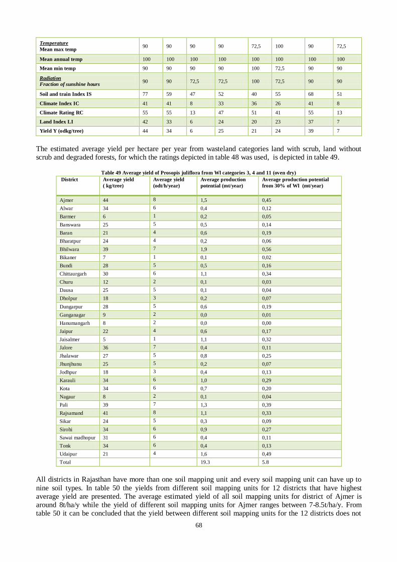
68

Temperature

Mean max temp 90 90 90 90 72,5 100 90 72,5

Mean annual temp 100 100 100 100 100 100 100 100

Mean min temp 90 90 90 90 100 72,5 90 90

Radiation

Fraction of sunshine hours 90 90 72,5 72,5 100 72,5 90 90

Soil and train Index IS 77 59 47 52 40 55 68 51

Climate Index IC 41 41 8 33 36 26 41 8

Climate Rating RC 55 55 13 47 51 41 55 13

Land Index LI 42 33 6 24 20 23 37 7

Yield Y (odkg/tree) 44 34 6 25 21 24 39 7

The estimated average yield per hectare per year from wasteland categories land with scrub, land without scrub and degraded forests, for which the ratings depicted in table 48 was used, is depicted in table 49.

Table 49 Average yield of Prosopis juliflora from Wl categories 3, 4 and 11 (oven dry)

District Average yield

( kg/tree)

Average yield

(odt/h/year)

Average production

potential (mt/year)

Average production potential

from 30% of Wl (mt/year)

Ajmer 44 8 1,5 0,45

Alwar 34 6 0,4 0,12

Barmer 6 1 0,2 0,05

Banswara 25 5 0,5 0,14

Baran 21 4 0,6 0,19

Bharatpur 24 4 0,2 0,06

Bhilwara 39 7 1,9 0,56

Bikaner 7 1 0,1 0,02

Bundi 28 5 0,5 0,16

Chittaurgarh 30 6 1,1 0,34

Churu 12 2 0,1 0,03

Dausa 25 5 0,1 0,04

Dholpur 18 3 0,2 0,07

Dungarpur 28 5 0,6 0,19

Ganganagar 9 2 0,0 0,01

Hanumangarh 8 2 0,0 0,00

Jaipur 22 4 0,6 0,17

Jaisalmer 5 1 1,1 0,32

Jalore 36 7 0,4 0,11

Jhalawar 27 5 0,8 0,25

Jhunjhunu 25 5 0,2 0,07

Jodhpur 18 3 0,4 0,13

Karauli 34 6 1,0 0,29

Kota 34 6 0,7 0,20

Nagaur 8 2 0,1 0,04

Pali 39 7 1,3 0,39

Rajsamand 41 8 1,1 0,33

Sikar 24 5 0,3 0,09

Sirohi 34 6 0,9 0,27

Sawai madhopur 31 6 0,4 0,11

Tonk 34 6 0,4 0,13

Udaipur 21 4 1,6 0,49

Total 19.3 5.8

All districts in Rajasthan have more than one soil mapping unit and every soil mapping unit can have up to

nine soil types. In table 50 the yields from different soil mapping units for 12 districts that have highest average yield are presented. The average estimated yield of all soil mapping units for district of Ajmer is around 8t/ha/y while the yield of different soil mapping units for Ajmer ranges between 7-8.5t/ha/y. From table 50 it can be concluded that the yield between different soil mapping units for the 12 districts does not

69

differ much. The largest difference between the soil mapping units can be seen for the districts of Karauli,

Kota and Swai madhopur. Since the wastelands are scattered all over the districts, therefore one cannot assign one soil mapping unit or soil type to wasteland categories land with scrub, land without scrub and degraded forests.

Table 50 Yield of Prosopis juliflora per soil mapping unit for 12 districts with highest average yield

Yield (t/ha/y)

3541 3677 3678 3686 3714 3716 3797 3809 3840 3859 3861 3878 6673 Yield range

(t/ha/y)

Ajmer 8.1 8.5 7.0 8.4 7 - 8.5

Alwar 6.1 5.1 5.9 6.2 5.1 - 6.2

Bhilwara 7.3 7.6 6.0 6 -7.6

Chittaurgarh 5.9 4.9 4.4 4.1 4.1 - 5.9

Jalore 5.8 6.9 5.8 - 6.9

Karauli 7.3 5.3 6.2 6.5 5.3 - 7.3

Kota 8.4 7.5 6.3 6.3 -8.4

Pali 6.9 6.1 7.2 6.1 - 7.2

Rajsamand 7.7 6.8 6.8 - 7.7

Sirohi 5.4 6.4 5.4 - 6.4

Sawai

madhopur

6.2 5.0 5.8 5.5 4.3 4.3 -6.2

Tonk 6.2 6.5 6.2 - 6.5

Based on the obtained results depicted in table49, Ajmer has the highest yield and the district of Bikaner has the lowest yield per hectare. Comparing the estimated yields with the yields of Prosopis juliflora form trial plantations in arid part of Rajasthan, the estimated yield in kg/tree is much lower. The reason could be because

the number of plants per hectare is usually low for trial plantations and plants are provided additional water and fertilizer see table 17. Yield of Prosopis juliflora in India is assumed to be between 11-20 tonne per hectare per year while elsewhere it is between 0.5-39 tonne per hectare per year. Lower yields of around 0.6-1.8 tonne per hectare per year for regions with an annual rainfall of lower than 300mm have also been reported. Barmer, Bikaner, Jaisalmer, Nagaur, Ganganagar and Hanumangarh are among the districts with annual rainfall lower than 300mm. The

estimated yield for the mentioned districts falls in the range of reported yield from regions with low rain fall. Due to large extent of available wasteland, the estimated potential of biomass from wasteland of Jaisalmer per year is high. Plantation of Prosopis juliflora in Jaisalmer might not be economical because the yield per hectare is low. The estimated average yield form other districts is lower than the reported yield of 11-20 tonne per hectare per year for India. However, it is possible that the reported yield of 11-20 tonne per hectare per year is for regions in India where the annual rainfall is higher Rajasthan.

According to Biofuel Authority of Rajasthan, maximum 30% of available wasteland can be allotted to government undertakings and companies (Gov of Raj. 2013b). The biomass potential from wasteland categories: land with open scrub, land with dense scrub and degraded forests is around 19 million tonne per year. Presumably 30% of the wasteland is available for plantation of Prosopis Juliflora. Based on stated 30% availability of wasteland, around 5.8 million tonne biomass (oven dry) can be supplied from wasteland per year. According to BRAI, the surplus of biomass from wasteland of Rajasthan is around 4.2 million per year. The estimated potential is much higher than the potential given by BRAI.

The biomass potential from wasteland categories sand-dunes and sands-desertic is presented in table 51. As expected the yields from wasteland categories sand-dunes and sands-desertic are much lower than wasteland categories land with scrub and degraded forests.

70

Table 51 Biomass yield from Wl categories 17-19 (Oven dry)

Yield Y

( kg/tree) Yield t/ha Yield t/ha /y Yield kt/y Yield kt/y ( 30% Wl )

Ajmer 27 11 1.8 2 0.9

Barmer 5 2 0.3 94 28.3

Bikaner 5 2 0.3 253 82

Churu 9 4 0.6 3 1

Ganganagar 7 3 0.5 53 18

Hanumangarh 7 3 0.5 11 4

Jaipur 17 7 1.1 1 0.3

Jaisalmer 5 2 0.4 433 130

Jalore 27 11 1.8 67 24

Jhunjhunu 22 9 1.5 2 0.7

Jodhpur 15 6 1.0 247 74

Nagaur 6 3 0.4 8 2.6

Pali 21 8 1.4 0 0.2

Sikar 22 9 1.5 6 2

Sirohi 27 11 1.8 7 3

Total (mt/y) 1.2 0.4

The yield in kg/tree is around 27kg for sand-dunes and sands-desertic in Ajmer while it is 44kg/tree for wasteland categories land with scrub and degraded forests. Ajmer, Jalore, Sirohi, Jhunjhunu and Pali are the only districts with high yield per tree for sand-dunes and sands-desrtic. These districts have a better climate than the districts like Bikaner, Barmer and Jaisalmer. Compared to yields depicted in table 17, the given yields in table 48 are much lower. The yields depicted in table 44 are from plantation trials of sandy soils, but the difference in yield could be because of the use of fertilizers and supplementary water.

If the coal-based power plants replace around 10% of their coal requirement with biomass, around 2.1 million tonnes of biomass would be needed per year. The total biomass required for biomass-based power plants is around 0.46 million tonnes per year. This means enough biomass can be supplied from plantation of wasteland categories under this study to meet the required annual biomass usage of mentioned power plants in chapter one.

71

7.2 Cost of biomass production district-wise

The estimated cost of production (COP) of biomass production ranges between $2-13.3/GJ. The COP of biomass is lowest for the district of Ajmer due to higher yield per hectare while in district of Jaisalmer production cost is the highest as a result of low yield per hectare, see table 52. The cost of production is low in districts located in the east of Rajasthan, while it is quite high in districts located in the west part of the state

Rajasthan. Table 52 Cost of production for average biomass yield

District COP ($/GJ) District COP ($/GJ)

Ajmer 2 Jaipur 3.4

Alwar 2.4 Jaisalmer 13.3

Barmer 10.8 Jalore 2.3

Banswara 3 Jhalawar 2.9

Baran 3.6 Jhunjhunu 3.1

Bharatpur 3.2 Jodhpur 4.1

Bhilwara 2.2 Karuali 2.4

Bikaner 8.9 Kota 2.4

Bundi 2.8 Nagaur 8.3

Chittaurgarh 2.7 Pali 2.2

Churu 6.1 Rajsamand 2.1

Dausa 3.1 Sikar 3.2

Dholpur 4.1 Sirohi 2.4

Dungarpur 2.9 Sawai madhopur 2.6

Ganganagar 7.4 Tonk 2.4

Hanumangarh 8.2 Udaipur 3.6

The cumulative biomass potential from wasteland categories land with open scrub, land with dense scrub and degraded forests of Rajasthan against the COP is illustrated in figure 18. Bellow COP of $3/GJ, the biomass potential is around 59PJ per year and a potential of 89PJ per year can be produced bellow $4/GJ. The total

available potential below $13.3/GJ is about 105PJ per year. The potentials shown in figure 26 can be generated if 30% of mentioned wasteland categories are planted with Prosopis juliflora.

Figure 26 Biomass potential and cost of production

The price of coal in India is depicted in table 50. The price ranges between 0.8 and 3.2 $/GJ, the higher the

gross calorific value the higher the price, see Appendix XIX. The price of coal per GJ for lower grade is much lower than the cost of production for biomass. According to Rajasthan State Mines and Minerals Limited, lignite or brown coal mines are in two districts of Rajasthan namely Barmer and Nagaur with a calorific value of 11 to 14 GJ/tonne. The price for coal with a calorific value of 11 to 14 GJ per tonne was between 0.8 - 0.9$ /GJ in 2012.

72

Chhabra thermal power plant uses coal with a calorific value 3500 kcal/kg which falls under coal grade 13.

The price of coal grade 13 is between 0.8-0.9$/GJ. For other three coal-based power plants in Rajasthan, information on calorific value of used coal was not available. However, most of the coal-based power plants in India use low grade coal.

Table 53 Price of coal $/GJ (HHV)

Grade GCV bands (GJ/tonne) Price (Rs./tonne) Price ($/tonne) Price ($/GJ)

G2 28 - 29 4870 90,2 3.1 – 3.2

G3 27 - 28 4420 81,9 2.9 – 3.1

G4 26 - 27 3970 73,5 2.7 – 2.9

G5 24 - 26 2800 51,9 2 – 2.1

G6 23 - 24 1740 32,2 1.3 – 1.4

G7 22 - 23 1520 28,1 1.2 – 1.4

G8 21 - 22 1370 25,4 1,2

G9 19 - 21 1060 19,6 1

G10 18 - 19 940 17,4 0.9 – 1

G11 17 - 18 770 14,3 0.8 – 0.9

G12 15 - 17 720 13,3 0.8 – 0.9

G13 14 - 15 660 12,2 0.8 – 0.9

G14 13 - 14 600 11,1 0.8 – 0.9

G15 12 - 13 550 10,2 0.8 – 0.9

G16 10 - 12 490 9,1 0.8 – 0.9

G17 9 - 10 430 8,0 0.8 – 0.9

Source: (CIL. 2013)

On behalf of Rajasthan Renewable Energy Corporation Limited (RREC) a study was conducted on supply of biomass in the state of Rajasthan. In this study a survey was conducted among farmers and biomass traders to find the price of biomass, namely crop residue and Prosopis juliflora. The average selling price of mustard

husk by farmers and traders is depicted in table 50. The average farmer’s price of mustard husk is lowest in Jhalawar with 1.3$/GJ and highest for the district of Jaipur. Comparing to COP biomass, the price of mustard husk is much lower in districts like Ganganagar, Hanumangarh and Jaisalmer. On the other hand the price is somewhat higher in districts like Ajmer, Alwar and Jalore.

Table 54 Average farmer selling price of mustard husk

District Price ($/GJ) District Price ($/GJ)

Farmers Traders Farmers Traders

Ajmer 2.6 3.1 Jaisalmer 1.5 N.A

Alwar 2.5 3.1 Jalore 3.1 3.6

Baran 1.5 2.1 Jhalawar 1.3 1.6

Barmer 1.4 N.A Jhunjhunu 2.8 3.2

Bharatpur 1.4 2.3 Jodhpur 1.5 2.1

Bikaner 2.6 3.1 Karuali 1.9 2.7

Bundi 1.9 2.7 Kota 2.2 2.7

Churu 1.9 3.1 Nagaur 2.6 3.2

Dausa 2.7 3.1 Pali 2.6 3.3

Dholpur 2.1 3.2 Sikar 2.7 3.0

Ganganagar 2.7 3.5 Sirohi 3.1 3.2

Hanumangarh 2.7 3.5 Sawai Madhopur 2.6 3.5

Jaipur 3.2 4.4 Tonk 2.2 3.1

Source: (Gov of Raj. 2013b)

The price of mustard husk by farmers is lower than cost of production of biomass in some districts and higher in others, however the price of low grade coal/GJ is significantly lower than the COP of biomass from

plantation of wasteland. In the following paragraphs the cost of transportation and cost of selected supply chains at the power plant gate is presented. The price of traders for mustard husk is than compared to cost of supply chains.

73

7.3 Transportation cost of selected biomass supply chains

As discussed in chapter five, the cost of transportation by road is highly competitive in India. However, due to low cubic capacity of trucks transport rates can still be high for freight with low density. In this paper a cubic capacity of 100m3 was assumed which resulted in a lower transportation cost, see table 51. A truck with a maximum load capacity of 27 tonnes can only transport 21 tonnes of logs and only 17 tonnes of chips if the

volume is 40m3. This means if a much lower cubic capacity was assumed, the difference between cost of transportation for logs and pellets and dry chips would be have been more significant. The estimated cost of transportation is around $0.05t-1km-1. The cost of transportation by truck was taken from a study on road transport in India by World Bank in 2005. However, the very recent available freight rates29 between Jaipur, Rajasthan and Delhi, Chennai, Mumbai and Kolkata show that the cost of transportation was between $0.023 and $0.035t-1km-1.

Table 55 Cost of transportation for selected biomass supply chains

Logs chips Pellets

Maximum load (t) 27 27 27

Maximum load (m3) 100 100 100

Maximum load used (t) 27 24 27

Maximum load used (m3) 58 72 39

GJ transported /trip 340 302 437

1st transportation ($/t) 0.13

2nd transportation ($/t) 0.05

On the basis of a study conducted by RREC, the cost of transportation for Prosopis juliflora from the forest was approximately $14/tonne for a transportation distance of 75km. In that case, the cost of transportation was $0.18t-1km-1 which is almost four times higher than the calculated cost of 2nd transportation in this paper. The

reported cost of transportation for mustard husk was around 2.2-3.2$/tonne, but the transportation distance between biomass source and power plant was not given.

29

http://www.infobanc.com/logistics/logtruck.htm

74

7.3.1 Biomass supply to thermal power plants (Co-firing)

The cost of selected supply chains for the coal-based power plants from the districts with the lowest cost at the power plant gate are shown in table 56. It was assumed that per district not more than 30% of wasteland can be used for plantation. Therefore the biomass has to be supplied from more than one district to meet the required amount. The districts with the lowest cost of biomass supply to the four thermal power plants under the study are Ajmer, Bhilwara, Jhalawar and Kota. For the power plants in Baran, Kota and Jhalawar, supply

of biomass from Kota is the most economical option. However, not all the required biomass can be supplied from Kota. Therefore, biomass has also to be supplied from Bhilwara and Jhalawar. The capacity of all power plants and the annual required amount of biomass are depicted in table 41, chapter 6.

Table 56 Cost of selected supply chains for thermal power plants

In table 56 the cost of biomass supply from the above mentioned districts to the power plants are depicted. The figures below show the cost of biomass supply and cost of electricity production for all power plants. For biomass chips, the cost of pre-treatment consists of chipping and for pellets the cost of pre-treatment includes

chipping, drying, milling and pelletsing. The cost of electricity production for the four thermal power plants is depicted in table 57.The cost of conversion from logs and chips to electricity includes cost of pre-treatment required at the power plant.

Table 57 Cost of power production co-firing

Chhabra thermal power plant, located in the district of Baran, has a capacity of 500MW. Supply of biomass

from Jhalawar and Kota is the most economical option for this power plant, see table 56. Supply of biomass from all other districts to Chhabra power plant is less economical compared to the mentioned districts. .

Figure 27 Supply of biomass from Jhalawar

Figure 27 shows that supply of logs and chips is more economical than supply of pellets at the power plant gate. It can be seen that the cost of 2nd transportation is lower for pellets and highest for chips, however the lower transportation cost of pellets does not compensate for the cost of pre-treatment. The cost of biomass supply chains is $4.49/GJ, $4.77/GJ and $5.2/GJ for logs, chips and pellets respectively. Figure 28 shows the cost of biomass supply from Jhalawar. The cost of biomass supply is around $4.53/GJ, $4.8/GJ and $5.8/GJ

Power Plants district

Baran Kota Jhalawar Ganganagar

Logs ($/GJ) 4.5 3.4, 4.3 4, 4.7 6.1, 7.2

Chips ($/GJ) 4.8 3.5, 4.6 4.2, 5, 4.1 6.6, 7.8

Pellets ($/GJ) 5.2, 5.8 4.4, 5 4,8, 5.4, 4.9 6.3, 7.1

Supply district Kota &

Jhalawar

Kota &

Bhilwara

Kota, Jhalawar and

Bhilwara Ajmer & Bhilwara

Power Plants district

Baran Kota Jhalawar Ganganagar

Logs ($/MWhe) 69 58 62 82

Chips ($/MWhe) 70 59 63 85

Pellets ($/MWhe) 72 62 68 81

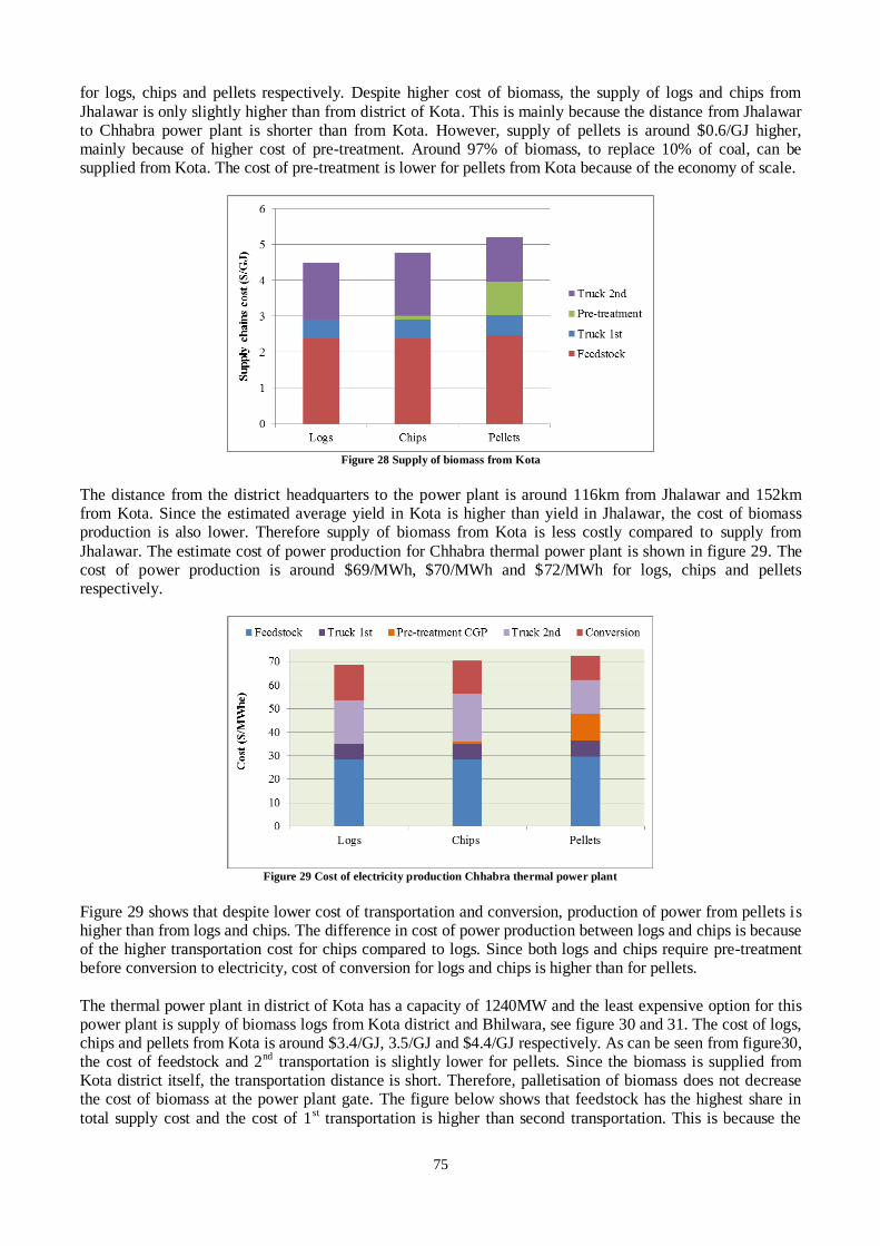
75

for logs, chips and pellets respectively. Despite higher cost of biomass, the supply of logs and chips from

Jhalawar is only slightly higher than from district of Kota. This is mainly because the distance from Jhalawar to Chhabra power plant is shorter than from Kota. However, supply of pellets is around $0.6/GJ higher, mainly because of higher cost of pre-treatment. Around 97% of biomass, to replace 10% of coal, can be supplied from Kota. The cost of pre-treatment is lower for pellets from Kota because of the economy of scale.

Figure 28 Supply of biomass from Kota

The distance from the district headquarters to the power plant is around 116km from Jhalawar and 152km from Kota. Since the estimated average yield in Kota is higher than yield in Jhalawar, the cost of biomass production is also lower. Therefore supply of biomass from Kota is less costly compared to supply from

Jhalawar. The estimate cost of power production for Chhabra thermal power plant is shown in figure 29. The cost of power production is around $69/MWh, $70/MWh and $72/MWh for logs, chips and pellets respectively.

Figure 29 Cost of electricity production Chhabra thermal power plant

Figure 29 shows that despite lower cost of transportation and conversion, production of power from pellets is higher than from logs and chips. The difference in cost of power production between logs and chips is because of the higher transportation cost for chips compared to logs. Since both logs and chips require pre-treatment before conversion to electricity, cost of conversion for logs and chips is higher than for pellets.

The thermal power plant in district of Kota has a capacity of 1240MW and the least expensive option for this power plant is supply of biomass logs from Kota district and Bhilwara, see figure 30 and 31. The cost of logs, chips and pellets from Kota is around $3.4/GJ, 3.5/GJ and $4.4/GJ respectively. As can be seen from figure30, the cost of feedstock and 2nd transportation is slightly lower for pellets. Since the biomass is supplied from Kota district itself, the transportation distance is short. Therefore, palletisation of biomass does not decrease the cost of biomass at the power plant gate. The figure below shows that feedstock has the highest share in

total supply cost and the cost of 1st transportation is higher than second transportation. This is because the

76

biomass is being supplied from Kota district and the cost of second transportation is higher than cost of second

transportation.


According to the estimated yield and production potential, only around 30% of biomass that is required to replace 10% of coal can be supplied from Kota district. After Kota, supply of biomass is economical from Bhilwara district. The cost of supply chains from Bhilwara is around $4.3/GJ for logs, $4.6/GJ for chips and $5/GJ for pellets. The difference in cost of supply logs and pellets from Kota is around $1.1/GJ, while from Bhilwara is only $0.7/GJ. This indicates a longer transportation distance which is also visible in figure 31. The 2nd transportation distance from Bhilwara is around 152km which is clearly much longer compared to the

transportation distance from Kota district. As can be seen from figure 31, the cost of second transportation from Bhilwara is much higher compared to figure 30.

Figure 31 Supply of biomass from Bhilwara

Despite the longer distance, supply of pellets from Bhilwara is economically less favourable compared to logs and chips from Bhilwara. Also in this case the lower cost of transportation does not compensate the cost of pre-treatment. Compared to figure 31, it can be seen that the share of second transportation is higher in supply cost due to longer transportation distance.

Figure 32 shows the cost of electricity production for Kota thermal power plant. The cost of electricity production from logs, chips and pellets is around $58/MWhe, $59/MWhe and $62/MWhe respectively. For logs and chips as well for pellets, cost of feedstock covers around 50% of the total production cost. The figure shows that the cost of electricity from logs is the lowest and highest from pellets.

77

Figure 32 Cost of electricity production for Kota thermal power plant

The Kalisindh thermal power plant is located in the district of Jhalawar. With a capacity of 1500MW, Kalisindh thermal power plant has the highest capacity among the four thermal power plants under the study. The most economical option for this thermal power plant is to supply logs from district of Kota, Jhalawar and Bhilwara. Supply of biomass from Kota is less costly compared to supply from districts of Jhalawar and Bhilwara. However, only around 38% of the required amount can be delivered from Kota.


The cost of biomass supply from Kota district is around $4/GJ for logs, $4.2/GJ for chips and $4.8/GJ for pellets, see figure 33. After Kota, supply of biomass is economical from district of Jhalawar. About 53% of the required biomass amount can be supplied from Jhalawar. The cost of biomass supply from Jhalawar is around $4/GJ, $4.1/GJ and $4.9/GJ for logs, dry chips and pellets respectively, see figure 34.

Figure 34 Supply of biomass from Jhalawar

78

Around 9% of the required biomass has to be supplied from another district. After Kota and Jhalawar, supply

of biomass from Bhilwara is the most economical option. The estimated cost of biomass supply from Bhilwara is around $4.7/GJ, $5/GJ and $5.4/ GJ for logs, chips and pellets respectively, see figure 35.


Compared to figure 33 and 34, the cost of 2nd transportation is higher in figure 35. This is because the distance between the district of Bhilwara and Kalisindh thermal power plant is longer. The distance from Kota to the

power plant is around 84km, 13km from Jhalawar and around 214km from Bhilwara. From the figures 33-35, it can be seen that the cost of feedstock is lowest in the district of Bhilwara. However, due to longer distance, the cost of second transportation is much higher which makes supply of biomass to Kalisindh power plant less economical compared to supply of biomass from districts of Kota and Jhalawar.

Figure 36 Cost of electricity production Kalisindh thermal power plant

The power plant in Suratgarh is located in district of Ganganagar, the north western part of the Rajasthan state

and has a capacity of 1200MW. The distance between Ganganagar and districts with low COP of biomass is much longer compared to the other power plants. Therefore, supply of biomass to Suratgarh thermal power plant in Ganganagar is higher than for other power plants, see figure 37. The most economical option for the power plant in Ganganagar is to supply logs from Ajmer and Bhilwara districts. The cost of biomass supply from Ajmer is around $6.1/GJ for logs, $6.6/GJ for chips and $6.3/GJ for pellets. The distance between Ajmer and Suratgarh thermal power plant is around 419km. Despite the long transportation distance, supply of logs is still economical at the power plant gate. However, due to the long transportation distance, the difference in cost of supply of logs and pellets are smaller.

79

Figure 37 Supply of biomass from Ajmer

Figure37 which illustrates the cost of biomass supply from district of Ajmer, clearly shows that cost of

transportation for pellets are lower than for logs and chips. However, the difference in cost of transportation of logs and pellets are slightly lower than the cost of pre-treatment making pellets less economical. Figure 38 shows the cost of supply from Bhilwara district. It can be seen that supply of pellets is less costly than logs and chips. The distance from Bhilwara to Suratgarh thermal power plant is around 543km which is longer than the transportation distance between Ajmer and the power plant in Ganganagar.


Figure 37 and 38 shows that the cost of second transportation covers more than the 50% of total supply cost

clearly showing that the biomass has to be supply over a long distance.

Figure 39 Cost of electricity production Suratgarh thermal power plant

80

The cost of electricity production for Suratgarh thermal power plant is shown in figure 39 and the cost of

electricity production is approximately $82/MWhe for logs, $85/MWhe for chips and $81/MWhe for pellets. Unlike figures 37 and 38, figure 39 shows that the cost of power production from pellets is more cost-effective than cost of production from logs. Economical feasibility to replace 10% coal with biomass depends on transportation distance of coal and the grade of coal being used. If coal transportation takes place by mean of railway, the cost of transportation would be around $0.02 t-1km-1 for coal from Barmer and Nagaur. The freight rate per tonne by railway and

general classification of goods can be found in Appendix XX. The total amount of required biomass for co-firing would be around 2.1 million oven dry tonne per year. According to the estimated costs of biomass supply chains for the four coal-based power plants, supply of logs is the cheapest option from the districts of Ajmer and Kota. When we compare the price of low grade coal with the production costs of biomass, the production costs of biomass is much higher. The of cost transportation for coal by railway is quite low which does not have any significant effect on the

final price delivered at the power plant gate. Since, the price of low grade coal and transportation costs is cheaper than the production and transportation costs of biomass. It is economically not feasible to replace 10% of coal for biomass co-firing. However, if thermal power plants are using high grade coal, coal grade 2 and 3, replacing of 10% coal would economically be feasible. For all coal-based power plants, the district-wise estimated cost of selected supply chains can be found in Appendix XXI.

7.3.2 Supply of biomass to biomass-based power plants

In this paragraph the cost of biomass supply chains to small scale biomass-based power plants is being discussed. The figures below show the supply of biomass and cost of electricity production for the power plants located in Baran, Ganganagar and Sirohi. The figures for all other power plants can be found in Appendices XXI and XXIII. The power plant in Baran has a capacity of 8MW and uses mustard husk as fuel. Assuming an efficiency of 25%, the total required biomass per year would be approximately 45 kilo tonnes. The supply of logs from Kota district is $4.1/GJ which is the most cost efficient option, see figure 31. Since biomass can be supplied

over short transportation distance and the difference in cost of transportation for logs and pellets is very small to compensate the cost of pre-treatment.

Figure 40 Cost of selected supply chains from Kota (Baran)

Farmers and traders ask $1.5/GJ and $2.1/GJ for mustard husk for the district of Baran. Compared to the price of traders for mustard husk which includes transportation cost, the cost of biomass logs at the power plant gate is $2.2/GJ higher. Figure 41 shows the cost of power production and as can be seen, production of power from logs is the lowest and from pellets the highest. The cost of power production is around $201/MWhe, $203/MWhe and $207/MWhe from logs, chips and pellets respectively.

81

Figure 41 Cost of electricity production power plant Baran

The biomass based power plant in the district of Ganganagar has a capacity of 7.8MW and uses mustard husk

and cotton stalk as fuel. The price of mustard husk including transportation cost is about $3.5/GJ, while supply of logs cost around $6.7/GJ. Figure42 shows that the cost of supply for pellets is higher than for logs and lower than chips. The figure also shows that the cost of 2nd transportation covers more than half of the supply cost for logs and chips.

Figure 42 Cost of selected supply chains from Alwar (Ganganagar)

Although figure 42 shows that the supply of logs is less costly compared to pellets, figure 43 shows that the cost of power production is the lowest from pellets which is approximately $233/MWhe against $236/MWhe and $242/MWhe for logs and chips.

Figure 43 Cost of electricity production power plant Ganganagar

82

The power plant in Sirohi has a capacity of 20MW and is the largest biomass-based power plant in the state

for Rajasthan. Hence, the cost of pellets is marginally lower than for other power plants but the supply of pellets is still not economical compared to logs, see figure 44. The COP of logs at the power plant gate is around $2.9/GJ.

Figure 44 Cost of selected supply chains (Sirohi)

Unlike the power plants in Baran and Ganganagar, biomass for the power plant in Sirohi can be supplied locally. Therefore, it was assumed that biomass logs can be supplied directly to the power plant. However, for pellets and chips, it was assumed that biomass would be gathered at CGP and supplied to power plant being pre-treated.

Figure 45 Cost of electricity production Sirohi power plant

The biomass based power plant in Sirohi has the highest capacity among the eight small scale power plants and therefore the cost of power production for all other small scale power plant is higher than the cost for power plant in Sirohi, see table 59. In table 58, the name of the districts from where the supply of biomass is the lowest are depicted. Supply of biomass from all other districts can be found in Appendix XXII. Supply of biomass and cost of electricity production for the power plants in Jaipur, Jalore, Kota, Nagaur and Tonk is shortly discussed below. In table 58 and 59 the cost of supply for logs and cost of electricity

production can be found. For the power plant in Jaipur and Nagaur, the supply of biomass is more cost efficient if supplied from districts of Alwar and Ajmer. For the power plants in Jalore, Kota and Tonk biomass can be supplied locally.

83

Table 58 Cost of logs supply and price of mustard husk

Power plant district Supply district Logs ($/GJ) Mustard husk traders ($/GJ)

Baran Kota 4.3 2.1

Ganganagar Ajmer 6.5 3.5

Jaipur Alwar 4 4.4

Jalore Jalore 2.8 3.6

Kota Kota 3.1 2.7

Nagaur Ajmer 3.5 3.2

Sirohi Sirohi 3.7 3.2

Tonk Tonk 3.7 3.1

In table 58 the cost of power production for all biomass based power plants are depicted. It can be seen that the cost of power production is the lowest if biomass is supplied as logs, except for the power plant located in the district of Ganganagar. The transportation distance between supply district and power plant district is too long and therefore supply of pellets is more economical.

Table 59 Cost of electricity production biomass based power plants

Power plant district Logs ($/MWhe) Chips ($/MWhe) Pellets ($/MWhe)

Baran 201 203 207

Ganganagar 236 242 233

Jaipur 196 197 203

Jalore 163 175 183

Kota 183 188 202

Nagaur 180 181 187

Sirohi 149 160 167

Tonk 181 193 201

The 8MW power plant in Jaipur district also uses mustard husk as fuel. The price of mustard husk for Jaipur is

around $4.4/GJ which is costlier than the supply of logs from district of Alwar. Logs from Alwar costs $4/GJ which is the most economical option. The cost of supply for chips and pellets can be found in the Appendix XXII. Table 59 shows that the cost of electricity production for the power plant Jaipur is around $196/MWhe from logs and around $203/MWhe from pellets. The cost of biomass logs for the 10MW power plant in Nagaur is is around $3.5/GJ and the cost of power production is around $180/MWhe. The 12MW power plant in district of Jalore uses Prosopis juliflora, groundnut shell and saw dust as fuel.

According to the study of RREC, Prosopis juliflora can be supplied by Agriculture department, State Forest Department and farmers to the power plants. The price of Prosopis juliflora is between 2.3-2.6$/GJ for logs and 2.7-2.9$/GJ for wood chips at the power plant gate. The cost of biomass supply from wasteland for district of Jalore is around $2.8/GJ for logs which is the cheapest option. Compared to the price of Prosopis juliflora the cost of biomass supply from wastelands is slightly higher. For the 8MW power plant in Kota, supply of biomass is cost efficient if supplied locally. The estimated cost

of logs at the power plant gate is $3.1/GJ. The price of mustard husk for Kota is around $2.1/GJ which is about $1/GJ lower than COP of biomass from wasteland. Tonk has a capacity of 8MW and uses mustard husk as fuel. The cost of logs at the power plant gate is approximately $3.4/GJ while the price of mustard husk is around $2.7/GJ. The cost of transportation for pellets is lower than the cost of transportation for logs; however the cost of pre-treatment is higher than the difference in cost of transportation. Therefore, supply of pellets is less economical than supply of logs for all the small scale biomass based power plants except the power plant located in the

district of Ganganagar. Also supply of biomass as chips is economically less favourable. Figure 40-45 show that the cost of transportation for pellets due to higher density is lower; however for chips the cost of transportation because of their lower density is higher than for logs. Therefore, chipping of biomass irrespective transportation distance only increases the cost of supply.

84

7.3.3 Large scale biomass power plant

Based on the estimated yield per year around 5.8 million oven dry tonne biomass can be supplied from plantation of 30% wasteland categories land with open scrub, land with dense scrub and degraded forests. Hence enough biomass can be produced to feed a large scale biomass power plant. The biomass power plant in Polaniec Poland has a capacity of 205MW. It is claimed to be the world largest

power plant with an efficiency of more than 36% (Foster-Wheeler. 2013). Ajmer, Bhilwara, Pali and Rajsamand are districts with highest yield per hectare. About 1.7 million oven dry tonne biomass can be supplied from 30% of wastelands in these four districts which can feed a power plant with a capacity up to 444MW assuming the same efficiency as the power plant in Polaniec Poland. If a 200MW power plant would be setup in one of the above mentioned districts, around 0.8 million oven dry tonne biomass would be required.

Figure 46 Wasteland in districts with highest biomass yield per hectare

In order to estimate the cost of biomass supply chains for a non-existing large scale power plant, it was assumed that the power plant would be located in the district of Ajmer. The biomass would be supplied from

Ajmer district and in case not enough biomass can be supplied from Ajmer, it would be supplied from Bhilwara and Rajsamand, see figure 56.

Figure 47 Supply of logs to Ajmer

85

The distance between the district headquarters was used as second transportation distance. The distance

between Bhilwara and Ajmer, and Rajsamand and Ajmer is around 135km and 215km respectively. Supply of logs at the power plant gate from the districts of Ajmer, Bhilwara and Rajsamand would cost around $2.5/GJ, $3.7/GJ and $4.2/GJ. Supply of logs from Bhilwara and Rajsamand is much costlier than from district of Ajmer mainly because of the cost of 2nd transportation, see figure 57. Since the biomass for the non-existing power plant has to be supplied from different districts, the cost of electricity production was estimated for logs, chips and pellets. Figure58 shows the cost of electricity

production for the large scale power plant and as it can be seen the most economical option is production of electricity from logs. The cost of power production is around $86/MWhe for logs, $88/MWhe for chips and $91/MWhe for pellets. As can be seen the cost of 2nd transportation and conversion is lower for pellets than for logs and chips. Yet the lower cost of 2nd transportation and conversion for pellets do not compensate for the cost of pre-treatment. Another disadvantage of pre-treatment is that biomass has to be supplied from different districts. If biomass is pre-treated before 2nd transportation the cost of pre-treatment is somewhat higher than when it is pre-treated at the power plant because of the economy of scale. Hence, it can be said

pre-treatment of biomass before transporting it to the power plant is not required since it does not decrease the cost of power production.

Figure 48 Cost of electricity production biomass based power plant

As mentioned above, supply of logs from Bhilwara and Rajsamand is more expensive than Ajmer. However, if a power plant would be located in such an area in Ajmer where large tracks of wasteland is available and is close to the districts of Bhilwara and Rajsamand, the cost of transportation would be much lower. Figure 59 shows a selected area located in districts of Ajmer, Bhilwara, Rajsamand and Pali. Around 1.2million oven dry tonne biomass can be supplied from that area. Thus, by locating a power plant in area where large tracks

wasteland is available, the transportation distance between biomass field and end destination would be much shorter leading to a lower cost of transportation.

7.4 Comparison between costs of electricity production

To compare the cost of power production between co-firing, large scale and small scale biomass-base power plant, the cost of power production for smallest thermal power plant in Baran, thermal power plant located in Ganganagar, a 200MW non-existing and 20 MW biomass-based power plant in district of Sirohi is compared. The cost of power production from logs and pellets for the above mentioned power plants are presented in

figure 49 and 50. The cost of electricity production from logs is around $149/MWhe for 20MW power plant in Sirohi, $86/MWhe for large scale power plant, $69MWhe for the thermal power plant in Baran and $82/MWhe for the power plant in Ganganagar.

86

Figure 49 Cost of power production from logs

Figure 59 shows that that the main difference between small scale biomass power plant, large scale biomass

power plant and co-firing is in cost of conversion. The cost of conversion is the lowest for the two thermal power plants and highest for the 20MW biomass based power plant in Sirohi. The cost of feedstock for 20MW power plant is the highest because of a lower efficiency compared to the large scale power plant and co-firing. Since a higher efficiency was assumed for the large scale biomass based power plant, the cost of feedstock is lower than for the co-firing. The cost of transportation is the lowest for the 20MW power plant, since biomass can be supplied locally. However for the thermal power plants in Baran and Ganganagar biomass has to be supplied from Kota and Ajmer, making the cost of transportation high. As can be seen, the cost of transportation for Baran is much lower compared to Ganganagar. This is because of the longer

transportation distance between Ajmer and Ganganagar. On the other hand, the cost of transportation for large scale biomass power plant is much lower since it was assumed that a power plant would be located in a district with high yield and low cost of production.

Figure 50 Cost of power production from pellets

In figure 61, the cost of power production from pellets for the above mentioned power plants is presented. The cost of electricity production from pellets is around $159/MWhe, $91/MWhe, $72/MWhe and $81/MWhe for

20MW, 200MW, 500MW co-firng and 1200MW co-firing respectively. The cost of biomass for all power plants under the study at the power plant gate is the lowest if biomass would be supplied as logs. The lower cost of transportation for pellets does not make them more economical than logs. However, when looking at the cost of power production, the cost of power production for the Suratgarh thermal power plant located in Ganganagar is more economical if pellets are used for power generation. Thus, supply of pellets compared to logs is not economical except for the Suratgarh thermal power plant located in the district of Ganganagar.

As expected the cost of power production is lowest for co-firing and highest for small scale biomass power plant. The cost of power production for large scale biomass-based power plant is higher than co-firing and lower than small scale biomass-based power plants. Therefore, the most economical option to increase share

87

of biomass based power is co-firing. The main difference in the cost of electricity production stems from cost

of conversion to electricity.

88

7.5 Sensitivity analysis

Sensitivity analysis for COP was performed for three parameters namely discount rate, labour wages and yield. The discount rate used in this study was 11.8% and sensitivity was performed for a range of 20% lower and up to 40 % higher discount rate.

Figure 51 Sensitivity analysis discount rate, labour wages and yield

Figure 44 shows sensitivity analysis of COP against percentile variation of discount rate, labour wages and yield. As expected the yield has the greatest influence on COP. COP changes drastically with the change in yield. With 20% higher yield, the cost of production decreases with more than 15%. Since the plantation is quite labour intensive in India, labour wages have also significant influence on the COP. However, labour

wages have less impact on COP compared to yield. Figure 44 illustrates that the percentile variation of discount rate has almost no impact on COP, unless the discount rate increases with high percentage to impact COP. With an increase of 40% discount the cost of production increases with only 8%. In Appendix XXIV district-wise sensitivity analysis for labour wages, yield and discount rate can be found. Regarding the yield per hectare, soil and terrain characteristics that have an impact are organic carbon level, gravel content and slope gradient. In table 60, the lowest and highest estimated yields per hectare are depicted.

Table 60 Highest and lowest estimated yield of Prosopis juliflora versus average yield (tonne/ha/year)

District Average yield Highest

estimated yield

Lowest

estimated yield


estimated

yield

Lowest

estimated

yield

Ajmer 8.2 8.4 2.7 Jaipur 4.1 5.6 0.8

Alwar 6.3 8.2 2.5 Jaisalmer 0.9 2.0 0.2

Barmer 1.2 1.9 0.3 Jalore 6.7 7.9 1.7

Banswara 4.7 7.4 0.8 Jhalawar 5.1 8.5 1.5

Baran 3.9 7.8 1.4 Jhunjhunu 4.7 6.3 0.9

Bharatpur 4.4 5.4 0.8 Jodhpur 3.4 5.0 0.7

Bhilwara 7.2 8.5 2.1 Karauli 6.4 8.4 1.1

Bikaner 1.3 1.9 0.3 Kota 6.4 9.5 0.9

Bundi 5.2 7.4 1.3 Nagaur 1.6 2.0 0.3

Chittaurgarh 5.5 8.5 1.6 Pali 7.2 7.4 1.5

Churu 2.2 2.8 0.9 Rajsamand 7.5 11.2 2.2

Dausa 4.7 5.3 0.9 Sikar 4.4 6.3 0.9

Dholpur 3.3 5.3 0.7 Sirohi 6.3 9.2 1.3

Dungarpur 5.1 9.5 1.5 Sawai

madhopur 5.8 8.9 1.7

Ganganagar 1.7 2.1 1.0 Tonk 6.2 7.4 1.9

Hanumangarh 1.6 2.1 0.7 Udaipur 3.9 8.4 1.7

89

The lowest possible yield is estimated by rating the lowest carbon level, highest slope gradient and gravel

percentage per district. The percentage of villages per district having a low carbon level is quite low and different wasteland categories are fragmented all over the area of the districts. Therefore, the average calculated yield was used to give a more accurate biomass production potential from wasteland categories under the study. In table 61 the highest and the lowest production potential from 30% of the three suitable wasteland categories are given. The estimated lowest production potential is around 1.6 million oven dry tonne biomass per year, which is significantly lower than the estimated average yield. However, as mentioned above, the lowest production potential is estimated by assuming the worst possible condition.

Table 61 District-wise production potential from 30 of Wl area (Million oven dry tonne per year)


estimated yield

Lowest

estimated yield


estimated

yield

Lowest

estimated

yield

Ajmer 0.45 0.46 0.15 Jaipur 0.17 0.24 0.03

Alwar 0.12 0.16 0.05 Jaisalmer 0.32 0.69 0.07

Barmer 0.05 0.08 0.01 Jalore 0.11 0.12 0.03


Baran 0.19 0.38 0.07 Jhunjhunu 0.07 0.10 0.01



Bikaner 0.02 0.03 0.01 Kota 0.20 0.30 0.03

Bundi 0.16 0.23 0.04 Nagaur 0.04 0.05 0.01


Churu 0.03 0.03 0.01 Rajsamand 0.33 0.50 0.10

Dausa 0.04 0.05 0.01 Sikar 0.09 0.14 0.02

Dholpur 0.07 0.12 0.02 Sirohi 0.27 0.40 0.06

Dungarpur 0.19 0.36 0.06 Sawai

madhopur 0.11 0.17 0.03

Ganganagar 0.01 0.01 0 Tonk 0.13 0.15 0.04

Hanumangarh 0 0.01 0 Udaipur 0.49 1.05 0.21

Total 5.8 8.7 1.6

In table 62, the estimated different scenarios are depicted. The table shows the yield for the lowest occurring

carbon level, highest gravel content and slope gradient and shows the impact of these factors on yield.

Table 62 Yield of Prosopis juliflora by varying the rating the most limiting factors (tonne/ha/year)

District Lowest

organic

carbon

Highest

occurring

gravel content

Highest

occurring slope

gradient

District Lowest organic

carbon

Highest

occurring

gravel

content

Highest occurring

slope gradient

Ajmer 4.5 8.2 2.7 Jaipur 2.6 3.4 1.5

Alwar 3.7 5.4 5.0 Jaisalmer 0.7 0.8 0.3

Barmer 0.9 1.0 0.4 Jalore 3.8 5.6 2.4


Baran 2.2 3.2 1.8 Jhunjhunu 2.8 4.2 1.7



Bikaner 0.8 1.2 0.5 Kota 3.5 5.2 2.1

Bundi 2.9 4.2 1.9 Nagaur 0.9 1.3 0.6


Churu 1.4 2.2 1.7 Rajsamand 4.2 6.1 3.4

Dausa 2.8 4.7 1.5 Sikar 2.8 3.8 1.6

Dholpur 2.0 2.7 1.5 Sirohi 3.6 5.1 2.8

Dungarpur 2.8 4.2 2.3 Sawai madhopur 3.3 4.7 2.6

Ganganagar 1.0 1.6 1.3 Tonk 3.5 6.2 2.3


In table 63, biomass production potential for the scenarios depicted in table 62 is given. The biomass potential is around 3.4million oven dry tonne per year when assuming that the wastelands have the lowest occurring

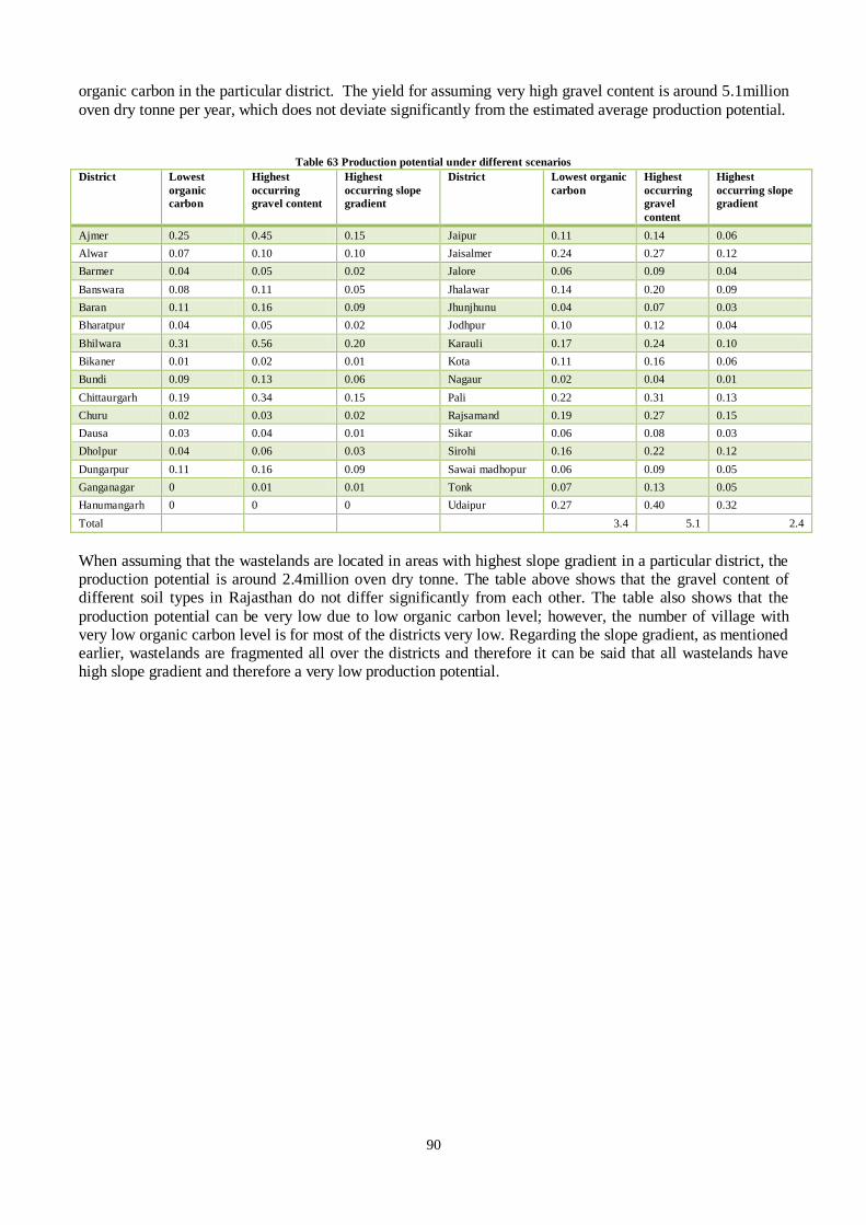
90

organic carbon in the particular district. The yield for assuming very high gravel content is around 5.1million

oven dry tonne per year, which does not deviate significantly from the estimated average production potential.

Table 63 Production potential under different scenarios

District Lowest

organic

carbon

Highest

occurring

gravel content

Highest

occurring slope

gradient

District Lowest organic

carbon

Highest

occurring

gravel

content

Highest

occurring slope

gradient

Ajmer 0.25 0.45 0.15 Jaipur 0.11 0.14 0.06

Alwar 0.07 0.10 0.10 Jaisalmer 0.24 0.27 0.12

Barmer 0.04 0.05 0.02 Jalore 0.06 0.09 0.04


Baran 0.11 0.16 0.09 Jhunjhunu 0.04 0.07 0.03



Bikaner 0.01 0.02 0.01 Kota 0.11 0.16 0.06

Bundi 0.09 0.13 0.06 Nagaur 0.02 0.04 0.01


Churu 0.02 0.03 0.02 Rajsamand 0.19 0.27 0.15

Dausa 0.03 0.04 0.01 Sikar 0.06 0.08 0.03

Dholpur 0.04 0.06 0.03 Sirohi 0.16 0.22 0.12


Ganganagar 0 0.01 0.01 Tonk 0.07 0.13 0.05

Hanumangarh 0 0 0 Udaipur 0.27 0.40 0.32

Total 3.4 5.1 2.4

When assuming that the wastelands are located in areas with highest slope gradient in a particular district, the production potential is around 2.4million oven dry tonne. The table above shows that the gravel content of different soil types in Rajasthan do not differ significantly from each other. The table also shows that the

production potential can be very low due to low organic carbon level; however, the number of village with very low organic carbon level is for most of the districts very low. Regarding the slope gradient, as mentioned earlier, wastelands are fragmented all over the districts and therefore it can be said that all wastelands have high slope gradient and therefore a very low production potential.

91

7.6 Discussion

7.6.1 Methodology

To accomplish this paper a comprehensive and well thought methodology was applied which is discussed in chapter 1. However, this paper and the methodology used have its limitation and shortcoming which is also discussed. To estimate the yield of Prosopis juliflora from wastelands specific soil and terrain, and climate characteristics were required. In general, wastelands have low nutrient value which makes them less suitable

for food crop production compared to agriculture land which has much higher productivity. Wastelands are fragmented all over the districts of Rajasthan. To rate the soil characteristics of each district, data of existing soil mapping units was extracted and all soil units/soil types of each soil mapping unit were rated. Subsequently, the average rating of all soil mapping units was used to estimate the yield from wasteland categories scrub land and degraded forests. The extracted data on physical and chemical characteristics of an area is not only from wasteland but it is also from non-wasteland areas. By not distinguishing in physical and

chemical attributes of wasteland and non-wasteland, one assumes that both land categories have the same productivities while there might be significant difference in productivities concerning Prosopis juliflora. The same land characteristics were assumed for different wasteland categories: land with scrub, land without scrub and degraded forest. Since mentioned wastelands belong to different wasteland categories, their physical and chemical characteristics might not be the same. To give a better yield estimation from these different categories and to be able to distinguish between their productivities, one should distinguish between their physical and chemical characteristics in different regions.

Physical and chemical characteristics of wasteland are rated roughly by using the average of soil mapping units. Yet, it can be argued that the adjusted methodology used in this study still provides reliable yield estimations from wastelands, because the tree species Prosopis juliflora can survive and thrive in poor soil and drought conditions. The wide adaptation of Prosopis juliflora is also visible from the rating of soil and terrain, and climate characteristics. For example, it does not matter whether the soil is excessively drained, somewhat excessively drained, well drained or moderately drained. It only makes a difference when the soil is imperfectly drained, poorly drained or very poorly drained. In Wasteland Atlas of India, land that is not

drained falls under wasteland category waterlogging. For wasteland categories land with scrub, land without scrub and degraded forests the drainage can be rated 100. Since, for every soil mapping unit an average rating of soil units/types was used, the soil units/types that are imperfectly drained, poorly drained and very poorly drained were not excluded. The rating of drainage for all the districts except Jalore is below 100. When looking only at the rating of drainage, it can be said that yield from the mentioned wasteland categories might be slightly higher because land that is not drained falls under wasteland category waterlogging.

Another land characteristic that has no significant impact on yield of Prosopis juliflora is the texture of soil. Out of 13 soil textures, 11 soil textures are rated 100, 2 are rated 90 and 2 are rated 72.5. It can be said that Prosopis juliflora grows on all soil types. The same applies on the cation exchange capacity of the clay fraction of the soil and when it is above 24, it is rated 100. Out of 23 soil-mapping units in the state of Rajasthan, only 1 soil-mapping unit has 2 soil units/soil types that have a cation exchange capacity of clay fraction below 24. Concerning the cation exchange capacity of clay fraction, it can be argued that it is not important to which soil units/soil types the different wasteland categories belong to. This is also the case for base saturation where soils having a base saturation of 50-100% is rated 100. Only one soil mapping unit have

two soil types with base saturation not falling in the range of 50-100%. The same argument is valid for total exchangeable base/cmol kg-1 soil, sodicity of soil and electrical conductivity of soil. There are only three soil mapping units that have one soil unit/ soil type with a very high electrical conductivity. These soil types are called Orthic Solonchalks and according to Wasteland Atlas of India, these soil types belong to wasteland category moderately saline/alkali land. Since, an average rate of the soil types was used, the electrical conductivity rating for the mentioned wasteland categories is below 100.

This means that estimated yield would have been somewhat higher if the Orthic Solonchalks was excluded from soil rating. To some extent, the pH of the soil has also less impact on yield and has no impact on the yield estimations in this study. Organic carbon level and pH of soil both fall under soil chemical characteristics. To calculate the soil and terrain index, only the most limiting factor under soil chemical

92

characteristics should be used in calculation. Since the organic carbon level is the most limiting factor under

soil chemical characteristics, the rating of pH was not used. The land characteristics that have an impact on yield estimation are the slope gradient, gravel content and organic carbon. By using an average rating for these characteristics, the estimated yields are either slightly on lower side or on a higher side. Since, land characteristics could not be solely extracted for specific wasteland category per soil mapping unit, it is difficult to say whether the estimated yield per hectare is on higher side or lower side from the actual yield.

Regarding the climate characteristics, average of mean max temperature, mean max annual temperature, mean minimum temperature, annual rainfall, length of dry season and fraction of sunshine per district were used. However, as can be seen from the annual rainfall map of Rajasthan in chapter 5, the rainfall in the western part of Jaisalmer district is lower than average and higher in the eastern part. A wasteland patch of category land with scrub in the west part of Jaisalmer district does not give similar yield as in the east part while in this study the estimated yield from land with scrub is the same whether it is located in the west of Jaisalmer or in

the east part of Jaisalmer. In order to point out high yield areas in a district, it is necessary to distinguish the yield of same wasteland category located in different parts of the district. This was not possible to achieve through this study because GIS was not used for yield estimations. In the cost estimation for biomass production, the costs of fertilizer and additional water were taken into consideration without taking the impact of fertilizer and supplementary water on yield from wasteland into consideration. If the impact of these two elements were taken into consideration the estimated yield could have been higher. As a result, a higher yield per hectare would lead to a lowers cost of production.

With regards to transportation costs, it was assumed that the biomass would be first transported to CGP in the district headquarter before being supplied to the thermal power plants within the district or other districts. However, in reality the CGP can be somewhere close to biomass field and does not have to be located in the district headquarters. Therefore, the actual cost of transportation to power plants could deviate from the estimated cost of transportation. Furthermore, the World Bank is the only body which has conducted a study on road transportation in India and it provided reliable information on transportation costs.

The main aims of this study were to provide insight into the extent and types of available wasteland, afforestation activities, in particular of wasteland and to estimate the biomass potential from afforestation of wasteland. In addition, the cost of four selected supply chains was estimated at the power plant gate. The calculated cost of power production for the power plants under the study was conducted only to compare the cost of power production between co-firing, small scale biomass based power plants and a non-existing large scale biomass power plant. Since, the cost of supply chains were calculated at the power plant gate, the cost of

storage was not taken into consideration. Therefore, the calculated cost of electricity production could be higher. Nevertheless, these cost calculations show significant difference between costs of electricity production of co-firing, small scale biomass based power plants and large scale biomass based power plant.

7.6.2 Data

The data on extent and categories of wasteland presented in Wasteland Atlas of India shows that there is a large area of wasteland available in India. The data on the extent of wasteland is very crucial for estimation of biomass potential from wastelands. Therefore, ground level data on the existence and availability of wasteland is required to give a more accurate estimation of biomass potential from plantation of wastelands. The three season satellite data presented in Wasteland Atlas of India was published in 2010. In a later project, the

change in area of different wasteland categories was measured and the results were published in Wasteland Atlas of India 2011. During the research on this paper more data were available. Also the web based GIS maps on wasteland, ground level water and slope gradient were available much later during this study. By the end of this study, data on road density and village connectivity was also available. Therefore, during the research certain assumption and methodology were adjusted and the content of research was extended. Detailed and specific data on past and current afforestation projects were not available either due to lack of

proper reporting or confidentiality of information. Therefore it was not possible to use plantation data such as yield and cost of plantation from past or on-going plantation projects. The obtained results show that the yield

93

of biomass is not the same in different districts of Rajasthan mainly due to different climate. Therefore, to

compare the estimated yield with actual yield, data on yield for different parts of Rajasthan is required. However, the available yield data from trial plantations is only for a few districts. In order to compare the estimate yield with actual yield, yield data for all districts for Rajasthan is needed which were not available. With regard to the cost of transportation, limited data was available on road transportation in India and the cost of transportation is only based on the study of World Bank. A reliable website provides information on freight rates per tonne for trucks with a capacity of 16 tonnes between major cities of India. Since, a truck

capacity of 27 tonnes was assumed in this study, the data provided on the road transportation by World Bank was used. This study provides the cost of transportation for trucks with a capacity of 9 tonnes, 16 tonnes and 27 tonnes. However, the associated cubic capacity of the trucks is not given. The study of World Bank indicates that the cubic capacity of the trucks in India is quite low with a maximum of 40m3. It should be noticed that the available sources do not provide relevant information about cubic capacity of the trucks in India. For a better cost estimation, it is essential to know whether the volume or

weight is the determining factors in transportation of biomass. If biomass is being transported with a truck that have a maximum capacity of 40m3, the cubic capacity would be the determining factor. A lower cubic capacity makes the cost of transportation in $/GJ for logs and wet chips slightly higher leading to a bigger difference between cost of transportation of the selected supply chains. Biomass based power plants can be found in all states of India; still there are no studies available on cost of transportation of biomass. The existing power plants and logistic companies are not keen on sharing any information concerning the price of feedstock, transportation and the like. Availability of information on transportation of

biomass would lead to better cost estimation of selected supply chains.

7.6.3 Comparison with other studies

The Biomass Resource Atlas of India has estimated the yield from wastelands in India. The estimated yield by Biomass Resource Atlas of India is quite low comparing with the yield from energy plantation estimated in this study. The estimated biomass potential from land with scrub, land without scrub and degraded forests is around 19.3 million tonnes if the total area under these categories would be used for plantation. The estimated potential from 30% of land is around 5.8 million tonnes. According to Biomass Resource Atlas of India, the total generated biomass from wastelands is around 6.7 million tonne per year from an area of 11mha and the

biomass surplus for power production is approximately 4.4 million tonnes per year. The main reason for this low potential could be that the Biomass Resource Atlas of India has considered wasteland as extension of forest. The estimations are based on the available species in forest and the yield from residues is used for the estimation of biomass potential from wastelands (CGPL. 2011; CGPL. 2010). Since, the yield of biomass depends on biophysical conditions, yield of Prosopis juliflora in Rajasthan might not be the same as in other parts of India. Consequently, the cost of biomass production might also not be the

same. To make a reasonable comparison of the obtained yield results with other studies or plantation projects, comprehensive data is required. Because no study on economical feasibility of large scale plantation of Prosopis juliflora could be found in India the calculated cost of plantation in this study cannot be compared.

7.6.4 Achievability of large scale plantation

According to recent data on wastelands, large areas of wastelands are available. Based on the obtained results from this study significant amount of biomass can be generated through plantation of these wastelands. However, availability of wasteland in government reports and the estimated biomass potential from wasteland do not say anything how realistic large scale plantation is. There are many other factors like wasteland ownership and connectivity of villages by road where wastelands are available which should be taken into

account. In this study, the yield was only estimated for one tree species while it is quite unrealistic to think that thousands hectares of wasteland would be covered with one species without any resistance from organisations protecting the environment. Degraded forests might still have many shrubs and other lower vegetation of food which might be wiped out by large scale monoculture plantation. Another issue is that the communities, living at the forest fringes depend on degraded forest for their livelihood and therefore large scale plantation might lead to opposition of local communities.

94

The web based GIS wasteland map shows that wasteland can be found in large patches. However, if

wastelands are fragmented in small patches across districts, the plantation activity would require more resources and time if it has to take place across different villages. Therefore, a clear picture of available wasteland per district is necessary which can be only achieved through ground level surveys. Implementing plantation activities on degraded lands that are fragmented over different village makes the management and control of it difficult which leads to a higher cost and would make wastelands less attractive for commercial plantation. Supply of biomass to the destination would also be a problem since biomass has to be gathered from different places.

In 2009, the National Policy on bio-fuels was adopted and a non-mandatory 20% blending of bio-diesel and bio-ethanol was proposed by 2017. The target is to be achieved through utilization of wastelands and fallow-lands for the cultivation of Jatropha curcas and Pongamia pinnata as the main feedstock for biodiesel. Under the Integrated Wasteland Development and other poverty alleviation programmes, around 2mha wasteland was assessed for plantation of Jathropha. Additionally, 4mha of government wasteland was assessed for plantation of Jathropha (PC. 2003; Centre for Jatropha Promotion. 2011).

The growth of Jatropha was promoted in different parts of the country in 2011 through various incentives. The most important characteristic of the bio-fuel program is to make only use of wastelands for plantation (Garg et al. 2011; Gunatilake et al. 2011). The growth of Jatropha on wasteland is also being promoted in Rajasthan and according to Biofuel Authority of Rajasthan maximum 30% of available wasteland can be used for government and companies undertaking (Gov of Raj. 2013b). On the other hand, the state government of Rajasthan has issued a policy to promote generation of electricity from biomass in 2010. In this policy, biomass from plantation of energy crops is also taken into consideration. This means that there would be a

competition in use of wasteland for plantation of biomass for electricity generation and Jatropha plantation to achieve the target of 20% non-mandatory blending (Gov of Raj. 2010; Gov of Raj. 2004). To determine the feasibility of large scale plantation, it is also important to include determinate issues discussed in this paper in future studies.

95

8 Conclusion and recommendation

8.1 Conclusion

To prevent further forest degradation and increase forest area through plantation, nationally and externally

aided social forestry and afforestation programmes were launched in India. The rate of return from social forestry programme like joint forest management was low. Mainly because of poor technology, poor seed quality, lack of post-plantation maintenance and the like. The forest policy in 1952 emphasized on bringing more than 30% of the geographical area of the country under tree cover by 2012. Despite annual plantation rate was too low to bring one third of the geographical area under tree cover, more than 42mha land was brought under tree cover between 1950 and 2011. Indian government put significant effort to prevent land degradation and increase tree cover and it can be

figured out from the number of programmes that have been launched so far. However, these programmes are not well organized and lack harmonization among various schemes. There have been efforts to tackle this issue and that is why, four centrally sponsored afforestation schemes were fused in one National Afforestation Programme to reduce multiplicity under the 9th five-year plan. Yet there exist different schemes with similar goals. The government of India also launched many wasteland development programmes to rehabilitate wasteland. Afforestation of wasteland is also taking place under these wasteland development programmes in order to meet the fuel-wood of rural community and to create rural employment.

Wasteland area was estimated by various agencies and the area ranged between 30-175mha. The most recent assessment of wasteland area for 2006 was conducted by National Remote Sensing Agency. Their estimation is the most accurate, reliable and detailed assessment till now since it is based on three season satellite data. The data on wasteland was also harmonized across databases in 2008 to give an accurate estimation. The recent estimations indicate a wasteland area of 47.2mha for 2006 and 46.7mha for 2009.

The two states with largest area of wasteland are Rajasthan and Jammu & Kashmir. Based on available data, out of 23 categories only 17 can be considered as marginally suitable, moderately suitable and suitable for plantation. Around 26mha of wasteland area, which is 57% of total wasteland area, consists of categories land with open scrub: land with dense scrub and degraded forests and these categories are suitable for plantation. Six wasteland categories were considered unsuitable for plantation. Nevertheless, the definition of wasteland by National Wasteland Development Board states that wastelands can be brought under vegetative cover with reasonable effort and the definition also applies on unsuitable wasteland categories like barren rocky areas. The area of wasteland in Rajasthan is approximately 8.5mha and around 4.7mha consists of wasteland

categories land with dense scrub, land with open scrub and degraded forests. Small scale plantations have taken place in India for the purpose of power generation either as main or secondary objective. However, it can be concluded that large scale plantation with dedicated energy crops to produce electricity has not taken place, because no such information was available on this subject. Yet the total biomass potential from wasteland as part of Biomass Resources Atlas of India project was estimated. Based on the estimation of this project, biomass power potential from wasteland is around 6.2GWe. Biomass

that can be generated from plantation of wasteland in Rajasthan is around 6.7 million tonne per year and the biomass surplus from wasteland is around 4.4 million tonne per year. Estimated biomass potential in this study from plantation of land with open scrub, land with dense scrub and degraded forests with Prosopis juliflora is around 19.3 million oven dry tonne per year. It was assumed that only 30% of wasteland under each category would be available for plantation. Therefore, a sustainable potential from the mentioned wasteland categories is around 5.8 million oven dry tonne per year. The highest

yield per hectare can be obtained from wastelands located in Ajmer and Rajsamand with 8 tonnes ha-1 year-1. The lowest yield is obtained from wastelands located in Jaisalmer and Barmer with 1 tonne per hectare per year. The cost of production from wasteland categories scrub land and degraded forests ranges between 2 to 15.8 $/GJ. The cost of production is lowest in district of Ajmer and highest in district of Jaisalmer. Biomass potential from plantation of wasteland categories sand-dunes and sands-desertic would be around 1.2 million tonne per year and 0.4 million tonne per year if only 30% of these categories would be used. The yield per hectare is 11 tonnes for districts of Ajmer and Sirohi, and 2 tonnes per hectare for Barmer, Bikaner and

96

Jaisalmer after a rotation cycle of six years. The Ministry of New and Renewable Energy considered these

wasteland categories suitable for energy plantation. Based on the result of this study, the yields from these categories are too low to use them for energy plantation. A very low yield implies a high cost of production per GJ and hence it is not economically feasible. With regard to transportation of biomass there are two main factors that were studied: transportation cost and road connectivity. Due to large number of small companies in transportation sector by road, the freight rates in India are among the lowest in the world. The state of Rajasthan has a road density of 0.55km per km2 which is

lower than national average of 1.25km per km2 despite being the largest state in the country. The percentage of villages with a population of 250-500 and below 250 people connected by road is very low. If wastelands are located in villages with low population, which is most likely the case, supply of biomass to power plants would be a challenge to overcome. On the other hand the road density has been increasing in India which might tackle village connectivity in the future. Nevertheless, it is very important to take village connectivity into account before establishing a plantation.

The estimated cost of transportation is around $0.05t-1km-1. The cost of transportation is quite low to have an impact on the delivered cost of biomass at the power plant gate. The cost of selected supply chains was estimated and since the cost of transportation is very low in India, pre-treatment only increases the cost of biomass at the power plant gate. It can be concluded that pre-treatment of biomass for the purpose of decreasing transportation cost is not a cost efficient choice, unless the transportation distance is above 500km. Compared to price of low grade coal, the cost of production of biomass is very high. The price of coal ranges between 0.8 and 3.2 $/GJ and most of coal based power plants in India use low grade cool. The price of low

grade coal is around 0.8$/GJ, while biomass logs cost 3.4- 7.2$/GJ for coal-based power plants if supplied from districts of Ajmer, Bhilwara, Jhalawar and Kota. The low grade coal is available in the state of Rajasthan and does not have to be supplied from other states. Even if it has to be supplied from other states, the cost of transportation of coal by railway is very low to have any impact on its price. Hence, replacing 10% of coal by biomass is economically not feasible for coal-based power plants unless high grade coal is being used for power production and /or coal is being transported over extremely long distances.

The cost of supply for logs for all biomass-based power plants, under the study is 3.1-6.5$/GJ if delivered from districts of Ajmer, Alwar, Kota, Jalore, Sirohi and Tonk. The price of mustard husk for these power plants ranges between 2.1-4.4$/GJ. Mustard husk can be supplied against lower price for all biomass based power except the power plant located in Jalore. Therefore, replacing crop residue with biomass delivered from wasteland is not economical for the biomass based power plants. Based on the district-wise estimated yield per hectare, the best location to setup a large scale biomass-based

power plant is between the districts of Ajmer, Bhilwara, Pali and Rajsamand. The yield per hectare is highest in these districts therefore the cost of production is the lowest compared to other districts. The supply of biomass logs would cost between 2.5 to 2.7$/GJ depending on the mentioned supply districts. The cost of power production is lowest for biomass co-firing and for all thermal power plants, except Suratgarh thermal power, the cost of production is the lowest if biomass is supplied as logs. The cost of power production from logs is around $69/MWhe for Chhabra thermal power plant, $58/MWhe for Kota thermal power plant, $62/MWhe for Kalisindh thermal power plant in Jhalawar district and $82/MWhe for Suratgarh

thermal power plant in Ganganagar. The estimated cost of electricity production for large scale biomass-based power plant is approximately $86MWhe for logs, $88/MWhe for chips and around $91/MWhe for pellets. The cost of power production for small scale biomass power plants is between 149 and 233$/MWhe. The cost of biomass for all power plants under the study at the power plant gate is the lowest if biomass would be supplied as logs. The lower cost of transportation for pellets does not make them more economical than logs. However, when looking at the cost of electricity production, pellets are more economical than logs for thermal

power plant in Suratgarh. Based on the results, it can be said that the best option to produce biomass-based power is co-firing. Not only from economical point of view as it was expected that co-firing is the most economical option, but also large amount of biomass-based power can be generated since the capacity of smallest thermal power plant is about

97

500MW. In addition, if biomass is not available coal-based power plants can still operate. The existing small

scale biomass power plants are already using surplus crop residues. Therefore, there is no need for energy plantation to meet their demand. Since, there is ambiguity on continuous availability of biomass in future; it is not a good option to setup a large scale biomass-based power plant to increase the share of biomass-based power.

8.2 Recommendation

In India, investments in afforestation projects are mostly undertaken by the government while the participation of private sector is negligible and most of afforestation programmes do not led to expected results. To implement the programmes successfully and achieve intended objectives, the government should involve private sector in afforestation of wasteland by leasing wasteland for commercial plantation with dedicated energy crops against a favourable price to make energy plantation for them economically feasible. Rajasthan has the capacity to produce significant amount of biomass from wasteland to replace 10% of annual

coal use of all its four coal-based power plants. Approximately 24% of plantation establishment costs, estimated in this study, consist of land cost. Therefore, leasing wasteland against an economical price for commercial plantation would drastically reduce the cost of biomass production. At the same time, wastelands that are not being used or are under-utilized would be reclaimed and used more productively. To claim large amounts of biomass that can be supplied from plantation of wasteland in Rajasthan requires more detailed en comprehensive research on the ownership of wasteland, current use and its impact on rural

communities. These are very important aspects that should be taken into consideration in order to obtain a more accurate estimation of available wasteland. According to definition of wasteland, wasteland is not being used or it is underutilized. But there is disagreement on the existence of wasteland as it has been argued that wasteland is being used in various ways by poor villagers. Therefore, for a better estimation more ground level data on the availability of wasteland is needed in order to avoid social conflicts with rural communities depending on common lands for their livelihood since the population is growing explosively in India. However, these aspects were not covered in this paper, because it

was beyond the scope of this paper. Further, in order to give more accurate estimation of biomass potential from wasteland, category-wise up to date data on the chemical and physical characteristics of wastelands is needed. Therefore, a database on soil properties of wasteland categories for every state is necessary to make more accurate estimation on availability of biomass in long term.

Although many forestry programmes with similar aim were merged by Ministry of Environment and Forests, there still exist many schemes with main objectives to increase tree cover and to meet the wood demand by plantation of wastelands. Ministry of Rural Development also have similar scheme with the same objective to reclaim wasteland through afforestation. Therefore, all the programmes targeting wasteland should be brought under one scheme in order to create a database with detailed data on categories of wasteland that are being planted, tree species used for plantation, cost of plantation and survival of plantation post establishment which will enable them to get a clear picture of wasteland plantation possibilities.

Last but not least, National Wasteland Development Board defines wasteland as degraded land that can be brought under vegetative cover with reasonable efforts and which is currently under-utilized and or/land that is deteriorating due to lack of appropriate water and soil management or due to natural causes. This definition refers to all categories of wasteland while there are categories like barren rocky area and glacial area that cannot be brought under vegetative cover with reasonable effort. Hence, this definition requires a revision and also more transparency should be provided on the definition of reasonable effort.

98

9 References

Baka, J. 2011. Biofuels and Wasteland Grabbing: How India’s Biofuel Policy is Facilitating Land Grabs in Tamil Nadu, India. Balooni, K. 2003. Economics of wastelands afforestation in India, a review. New Forests, 26, 101-136.

Balooni, K. & Singh, K. 2003. Financing of wasteland afforestation in India. 27, 235-246. Bansal, A., Chatterton, I., et al. 2005. India, Road Transport Efficiency Study. World Bank, Energy & Infrastructure Operations Division South Asia Regional Office. BERI. 2009. Biomass Energy for Rural India. World Wide Web Address: http://bioenergyindia.kar.nic.in/.

Bhumbla, D. R. & Khare, A. 1984. Estimate of Wastelands in India. Society for Promotion of Wastelands Development. Bohra, M. D., Harsh, L. N., et al. 1999. The Genus Prosopis: A Boon for Combating Desertification. September 1999, 3. CAZRI. 2009. Trends in Arid Zone Research in India. Central Arid Zone Research Institute, Jodhpur. Centre for Jatropha Promotion. 2011. The National Mission on Jatropha Biodiesel.

CGPL. Mapping of Bio-Waste Resources Across India. Combustion, Gasification & Propulsion Laboratory, Department of Aerospace Engineering Indian Institute of of Science. CGPL. 2010. Biomass Resource Atlas of India. World Wide Web Address: http://lab.cgpl.iisc.ernet.in/. CGPL. 2011. Biomass Resource Assessment. World Wide Web Address:

http://cgpl.iisc.ernet.in/site/BiomassAtlas/tabid/91/Default.aspx. CGWB. GW Profiles: District GW Brouchers Rajasthan. World Wide Web Address: http://cgwb.gov.in/District_Profile/Rajasthan_districtprofile.html. Chakraborty, D. 2010. Small holder’s carbon forestry project in Haryana India: issues and challenges. Mitigation and Adaptation Strategies for Global Change, 15, 899-915.

Chaudhary, A. P. C. 2011. New Delhi India,. CIFOR. 2009. Example of an afforestation/reforestation Clean Development Mechanism Project in Sisra, Haryana, India. Centre for International Forestry Research. CIL. 2013. Coal India Limited: Revised coal price with effect from 20 June 2012. World Wide Web Address: http://www.coalindia.in/Business.aspx?tab=2&AspxAutoDetectCookieSupport=1.

Damodaran, A. & Engel, S. 2003. Joint forest management in India: assessment of performance and evaluation of impacts. Discussion Papers, . DFID, HDRA, et al. Managing Prosopis Juliflora (Vilayati Babul) A Technical Manual.

Dhir, R. P., Kolarkar, A. S., et al. 1978. Soils of Rajasthan Desert and Their Characteristics. 44, 161-167. EPPI. 2011. Energy Plantation Project India. World Wide Web Address: http://www.eppi.co.in/index.php?page=concepts.

http://bioenergyindia.kar.nic.in/

http://lab.cgpl.iisc.ernet.in/

http://cgpl.iisc.ernet.in/site/BiomassAtlas/tabid/91/Default.aspx

http://cgwb.gov.in/District_Profile/Rajasthan_districtprofile.html

http://www.coalindia.in/Business.aspx?tab=2&AspxAutoDetectCookieSupport=1

http://www.eppi.co.in/index.php?page=concepts

99

FAO. 1985. Sand dune stabilization, shelterbelts and afforestation in dry zones

FAO Conservation Guide 10. Rome, Italy, . FAO, IIASA, et al. 2012. Harmonized World Soil Database (Version 1.2). World Wide Web Address: http://webarchive.iiasa.ac.at/Research/LUC/External-World-soil-database/HTML/. Foster-Wheeler. 2013. 205MWe Polanie Project: World’s Largest Biomass CFB Boiler Now in Commercial Operation.

Francescato, V. & Krajnc, N. 2009. Wood fuels handbook. AIEL-Italian Agriforestry Energy Association, . Ganapathy, J. 2011. Energy Plantation Project India. Garden-Organic. Managing Prosopis Manual. World Wide Web Address: http://www.gardenorganic.org.uk/pdfs/international_programme/ManagingProsopisManual.

Garg, K. K., Karlberg, L., et al. 2011. Jatropha production on wastelands in India: opportunities and trade-offs for soiland water management at the watershed scale. Goel, V. & Behl, H. 1998. Fuelwood quality of promising tree species for alkaline soil sites in relation to tree age. Biomass and Bioenergy, 10, 57-57-61. Gov of Raj. 2004. Policy for Promoting Generation of Electricity through Non-Conventional Energy Sources

2004. Government of Rajasthan, Energy Department. Gov of Raj. 2010. Policy for Promoting Generation of Electricity from Biomass 2010. Government of Rajasthan, Energy Department. Gov of Raj. 2011. Census of India 2011.

Gov of Raj. 2012a. Components of RACP. Department of Agriculture, Government of Rajasthan. Gov of Raj. 2012b. Minimum Wages. Government of Rajasthan, Labour Department. Gov of Raj. 2013a. Aravalli Afforestation Project. World Wide Web Address: http://rajforest.nic.in/?q=aravalli-afforestation-project.

Gov of Raj. 2013b. Biofuel Authority Rajasthan. World Wide Web Address: http://www.biofuel.rajasthan.gov.in/faq.html. Gov of Raj. 2013c. Draft Annual Plan 2013-2014: Transport and Communication. Gov of Raj. 2013d. Statistical Abstract 2011. World Wide Web Address: http://www.transport.rajasthan.gov.in/Statistical.htm.

Green, A. G. & Unruh, J. D. 2010. Clean Development Mechanism Afforestation and Reforestation projects: implications for local agriculture. CAB Reviews: Perspectives in Agriculture, Veterinary Science, Nutrition and Natural Resources, 5. Gunatilake, H., Sigyato, G., et al. 2011. Economy-Wide Impacts of Biodiesel Production and use in India: A Computable General Equilibrium Model Assessment. Asian Development Bank.

Hamelinck, C. N., Suurs, R. A. A., et al. 2005. International bioenergy transport costs and energy balance. Biomass and Bioenergy, 29, 114-134. Herath, G., Pohit, S., et al. 2011. Economy-Wide Impacts of Biodiesel Production and Use in India: A Computable General Equilibrium Model Assessment.

http://webarchive.iiasa.ac.at/Research/LUC/External-World-soil-database/HTML/

http://www.gardenorganic.org.uk/pdfs/international_programme/ManagingProsopisManual.

http://rajforest.nic.in/?q=aravalli-afforestation-project

http://www.biofuel.rajasthan.gov.in/faq.html

http://www.transport.rajasthan.gov.in/Statistical.htm

100

Hooda, N. & Rawat, V. R. S. 2006. Role of Bio-Energy plantations for carbon-dioxide mitigation with special reference to India. Mitigation and Adaptation Strategies for Global Change, 11, 437-459. ICRA. 2011. Spiralling Biomass Costs t Affect the Growth. Investment Information and Credit Rating Agency of India. IEA. 2009. World Energy Outlook 2009. International Energy Agency.

IEA. 2010. World energy outlook 2010. IEA (International Energy Agency), Paris, . IEA. 2011. Electricity/Heat Data for India. World Wide Web Address: http://www.iea.org/stats/electricitydata.asp?COUNTRY_CODE=IN. Indian-Bank. 2013. Lending Rates. World Wide Web Address: http://www.indian-bank.com/rate_loan.php.

India-WRIS WebGis. 2012. Water Resources Information System of India. World Wide Web Address: http://www.india-wris.nrsc.gov.in/. India-WRIS WebGis. 2013. LULC. World Wide Web Address: http://www.india-wris.nrsc.gov.in/LULCApp.html?UType=R2VuZXJhbA==?UName=. Inflation.eu. 2013. Inflation India. World Wide Web Address: http://www.inflation.eu/inflation-

rates/india/inflation-india.aspx. International Institute for Environment and Development. 2010. Biomass Energy – Optimising its Contribution to Poverty Reduction and Ecosystem Services. ISRO. 2013. Bhuvan Thematic Services. World Wide Web Address: http://bhuvan.nrsc.gov.in/bhuvan_links.php.

Jacobson, J., Jones, C., et al. 2005. Basic Soil Properties. Jagadish, K. 2003. Bioenergy for India: prospects, problems and tasks. Energy for sustainable development, 7, 28-34. Kalwar, S. C. 2008. Wastelands and Planning for Development. Concept Publishing Company, New Delhi,

India, . Kishore, V. V. N. 2011. New Delhi, India, . KRAJNC, N. Wood Energy Technologies. Lobo, V. 2011. SPWD. New Delhi, India, .

Maghembe, J. A., Kariuki, E. M., et al. 1983. Biomass and nutrient accumulation in young Prosopis juliflora at Mombasa, Kenya. Agroforestry Systems, 1, 313-321. Maps-of-India. 2009. Rajasthan District Map. World Wide Web Address: http://www.mapsofindia.com/maps/rajasthan/rajasthan.htm. Mehta, U. S. 2012. Research Study of the Road Transport Sector in India. Ministry of Corporate Affairs,

Government of India. Ministry of Finance. The Underlying Causes of Degradation.

http://www.iea.org/stats/electricitydata.asp?COUNTRY_CODE=IN

http://www.indian-bank.com/rate_loan.php

http://www.india-wris.nrsc.gov.in/

http://www.india-wris.nrsc.gov.in/LULCApp.html?UType=R2VuZXJhbA==?UName=

http://www.india-wris.nrsc.gov.in/LULCApp.html?UType=R2VuZXJhbA==?UName=

http://www.inflation.eu/inflation-rates/india/inflation-india.aspx

http://www.inflation.eu/inflation-rates/india/inflation-india.aspx

http://bhuvan.nrsc.gov.in/bhuvan_links.php

http://www.mapsofindia.com/maps/rajasthan/rajasthan.htm

101

MNRE. 2009a. Framework for MMATIC CDM Projects in Renewable Energy. Ministry of New and

Renewable Energy, Government of India. MNRE. 2009b. Report on Development of Conceptual Framework for Renewable Energy Certificate Mechanism for India. Ministry of New and Renewable Energy, Government of India. MNRE. 2010. BIOENERGY INDIA A QUARTERLY MAGAZINE ON BIOMASS ENERGY, PUBLISHED UNDER THE UNDP-GEF

BIOMASS POWER PROJECT OF MINISTRY OF NEW AND RENEWABLE ENERGY, GOVERNMENT OF INDIA. June 2010, . MNRE. 2011a. Draft Recommendations of Sub-Group on "Dedicated Energy Plantations and Forest Residues". Ministry of New and Renewable Energy, Government of India. MNRE. 2011b. A QUARTERLY MAGAZINE ON BIOMASS ENERGY, PUBLISHED UNDER THE

UNDP-GEF BIOMASS POWER PROJECT OF MINISTRY OF NEW AND RENEWABLE ENERGY, GOVERNMENT OF INDIA. January-March 2011, . MNRE. 2012. Biomass Resource Atlas. World Wide Web Address: http://mnre.gov.in/mnre-2010/schemes/resource-assessment/biomass-resource-atlas/. MOEF. 1988. National Forest Policy 1988. Ministry of Environment and Forests, Government of India.

MOEF. 2001a. National Action Programme to Combat Desertification in the Context of United Nations Convention to Combat Desertification. Ministry of Environment and Forests Government of India. MOEF. 2001b. State of Environment India. Ministry of Environment and Forests. MOEF. 2001c. Status of Forest in India. Ministry of Environment and Forests.

MOEF. 2006. Annual Report 2005-2006. Ministry of Environment & Forests, Government of India. MOEF. 2008. Mid Term Evaluation of the National Afforestation Programme. Ministry of Environment, Government of India. MOEF. 2010. National Mission for A Green India. Ministry of Environment and Forests.

MOEF. 2011a. Annual Report 2010-2011. Ministry of Environment and Forests, Government of India. MOEF. 2011b. India State of the Forest Report. Ministry of Environment and Forests, Government of India. MORD, D. 2010a. Annual Report 2009-2010. Ministry of Rural Development, Government of India. MORD, D. 2010b. Wastelands Atlas of India 2010. Ministry of Rural Development, Department of Land Resources, Government of India.

MORD, D. 2011. Wasteland Atlas of India 2011. Ministry of Rural Development, Department of Land Resources, Government of India. MORTH. 2011. Study on Economics of Trucking Industry. Ministry of Road Transport and Highways, Government of India.

MOSPI. Press Release on New CPI. World Wide Web Address: http://mospi.nic.in/Mospi_New/upload/new_cpi_18feb11.htm. MOSPI. 2013. Total and Surfaced Road Length. Ministry of Statistics and Programme Implementation, Government of India.

http://mnre.gov.in/mnre-2010/schemes/resource-assessment/biomass-resource-atlas/

http://mnre.gov.in/mnre-2010/schemes/resource-assessment/biomass-resource-atlas/

http://mospi.nic.in/Mospi_New/upload/new_cpi_18feb11.htm

102

MSPI. 2008. Twenty Point Programme-2006 Guidelines. Ministry of Statistics and Programme

Implementation, Government of India. NABARD. 2007. Forestry Wasteland, Forest Nursery. World Wide Web Address: http://www.nabard.org/modelbankprojects/forestry_nursery.asp. NAEB. 2010a. Reports-Statistics at a Glance: NAP Area. New Delhi, India, 2012. NAEB. 2010b. Schemes, Programmes and other Activities: 20 Point Programme. New Delhi, india, 2012.

OALD. 2011. Oxford Advanced Learner's Dictionary. World Wide Web Address: http://oald8.oxfordlearnersdictionaries.com/dictionary/wasteland. Palm, M. 2011. Rehabilitating Indian wasteland - a role for afforestation. Pandey, A., Bhargava, P., et al. 2010. Performance of Jatropha curcas: a biofuel crop in wasteland of Madhya

Pradesh, India. Journal homepage: www.IJEE.IEEFoundation.org, 1, 1017-1026. Pasiecznik, N. M., Felker, P., et al. 2001. The'Prosopis Juliflora'-'Prosopis Pallida'Complex: A Monograph. HDRA Coventry, . PC. 2001. Report of the Task Force on Greening India for Livelihood Security and Sustainable Development. Planning Commission, Government of India.

PC. 2002. Tenth Five Year Plan. Planning Commission, Government of India. PC. 2003. Report of the Committee on Development of Bio-Fuel. Planning Commission, Government of India. PC. 2005. Draft Report of the Expert Committee on Integrated Energy Policy. Planning Commission, Government of India.

PC. 2006a. Rajasthan Development Report. Planning Commission, Government of India. PC. 2006b. Report of Working Group on Forests for the Eleventh Five Year Plan (2007-2012). Planning Commission, Government of India. PC. 2008. Eleventh Five Year Plan. Oxford University Press.

PISCES RPC Consortium. 2011. Bioenergy Resource Status in India. M.S Swaminathan Research Foundation. Ramachandra, T. V. & Kamakshi, G. 2005. Bioresource Potential of Karnataka(Talukwise Inventory with Mangement Options). Ravindranath, D. 2011. Bioenergy for Rural India, Carbon Mitigation Report. UNDP.

Ravindranath, N. H. & Hall, D. O. 1995. Biomass, energy and environment: a developing country perspective from India. Oxford University Press, . Ravindranath, N. & Balachandra, P. 2009. Sustainable bioenergy for India: Technical, economic and policy analysis. Energy, 34, 1003-1013.

Ravindranath, N., Chaturvedi, R. K., et al. 2008. Forest conservation, afforestation and reforestation in India: Implications for forest carbon stocks. Current science, 95, 216-222. Ravindranath, N. & Murthy, I. 2010. Greening India Mission. Current Science(Bangalore), 99, 444-449.

http://www.nabard.org/modelbankprojects/forestry_nursery.asp

http://oald8.oxfordlearnersdictionaries.com/dictionary/wasteland

103

Ravindranath, N., Sudha, P., et al. 2001. Forestry for sustainable biomass production and carbon

sequesteration in India. Mitigation and Adaptation Strategies for Global Change, 6, 233-256. RPCB. State Environmental Atlas Rajasthan. Rajasthan State Pollution Control Board. RRECL. 2013. Details of Commissioned Biomass Power Projects. Rajasthan Renewable Energy Corporation. RVUN. 2013. World Wide Web Address: http://www.rvunl.com/Index.php#.

Saigal, S. 2011. Greening the'Wastelands': Evolving Discourse on Wastelands and its Impact on Community Rights in India. Saxena, S. K. 1998. Ecology of Prosopis juliflora in the arid regions of India. Saxena, V. P. C. 2011. New Delhi, India, .

Seshadri, C. V., Venkataramani, G., et al. 1978. Monograph Series On ´ Engineering of Photosynthetic System´ Energy Plantations´- A case Study for the Coromandel Littoral. 2. Sharma, R. D. 1992. Economics of fuelwood production in wastelands. Concept Publishing Company, .

Shrivastava, A. K. 2007. Environment Monitoring and Evaluation. A P H Publishing Corporation, New Delhi, India, . Singh, G. 1998. Practices for raising Prosopis plantations in saline soils. Singh, G. 2008. Managing Prosopis for Livelihood Security in Salt Affected and Dry Areas. Central Soil Salinity Research Institute.

Singh, J. V. Rehabilation of Degraded Rangelands and Stabilization of Production in Arable Arid Land of Thar Desert, India. 2013. Sirmah, P., Muisu, F., et al. 2008. Evaluation of Prosopis juliflora properties as an alternative to wood shortage in Kenya. Bois et Forêts des Tropiques, 298, 25-35.

SPWD. 2009. Wastelands News. XXIV, 26. Srinivas, S. N. 2011. Biomass Energy for Rural India. New Delhi, India, . Stewart, R. 1981. Modelling Methodology for Assessing Crop Production Potentials in Canada. , 29. Stille, L., Smeets, E., et al. 2011. The economic performance of four (agro-) forestry systems on alkaline soils in the state of Haryana in India. Energy for Sustainable Development, 15, 388-397.

Sudha, P., Somashekhar, H., et al. 2003. Sustainable biomass production for energy in India. Biomass and Bioenergy, 25, 501-515. Suresh, D. R. 2011. Suresh Forestry Network. The Indian Express. 2011. To Add to City's Water Woes, Tanker Operators Hike Prices. The Indian Express,

News. Tradings-Economics. 2013. India-National Statistics. World Wide Web Address: http://www.tradingeconomics.com/india/indicators.

http://www.rvunl.com/Index.php

http://www.tradingeconomics.com/india/indicators

104

Trivedi, T. P. 2010. Degraded and Wastelands of India

Status and Spatial Distribution. Indian Council of Agricultural Research, New Delhi India, . Vashev, B., Gaiser, T., et al. 2010. Biosafor Project Deliverable 9: Remediation of Saline Wastelands through the Production of Bioasaline Biomass (for Bioenergy, Fodder and Biomass). University of Hohenheim, Hohenheim, Germany. Wani, S. P. & Sreedevi, T. K. 2005. Pongamia's Journey from Forest to Micro-Enterpise for Improving

Livelihoods. International Crops Research Institute for the Semi-Arid Tropics. Wicke, B., Smeets, E., et al. 2011. The global technical and economic potential of bioenergy from salt-affected soils. Energy Environ.Sci., 4, 2669-2681. Williams, J. 2001. Financial and other incentives for plantation establishment. , 87-101.

Wright, J. E. 2010. Literature Review of Woody Biomass and Land Use Potential for Community Management in India. Yamashita et al. 2001. Afforestation Project in Aravalli Hills.

105

10 Appendices

10.1 Appendix I Wasteland Rajasthan

Table I 1 District and category wise wastelands of Rajasthan

Ajmer Alwar Barmer Banswara Baran Bharatpur Bhilwara Bikaner Bundi Chittaurgarh Churu Dausa Dholpur Dungarpur Ganganagar Hanumangarh

Wl cat.

1 34 45 0,5 0 73 3 12 58 81 0,1 4 9 75 0 0 0

2 0 40 19 0 39 0,2 0 35 191 0 0 3 31 0 0 0

3 559 496 619 172 291 277 1406 132 255 771 150 192 344 400 76 24

4 1076,7 51,3 719,5 176,7 165,9 134,8 814,3 398,3 82,9 388,5 241,0 64 96 551 81 41

5 8,6 0,0 0,2 0,0 0,0 0,0 0,0 0,4 0 0 1,3 0 0 0 7 7

6 0 0 21 0 0 8 0 0 0 0 0 0 0 0 7 1

7 10,8 0,2 105,3 0 0 0,3 0 0 0 3 15 0 0 0 0 0

8 18 0 3 0 0 0 0 0 0 0 0 0 0 0 0 0

9 0 0 0 0 0 0 0 0 0 0 0 0 0 0 0 0

10 0 0 0 0 0 0 0 0 0 0 0 0 0 0 0 0

11 200 98 113 628 1160 40 352 70 717 902 0 64 294 311 0 23

12 0 10 0 15 7 0 3 1 1 5 0 1 1 18 0 0

13 88 0,1 156 19 96 0 313 466 26 49 130 11 0 26 0 11

14 0,1 0 0 0 0 0 0 0 0 0 0 0 0 0 0 0

15 0,1 0,1 2,3 0 40 0 0 0 0 0 0 0,5 0,2 0 0 0

16 0 0 0 0 0 0 0 0 0 0 0 0 0 0 0 0

17 13 0,1 160 0 0 1 0 952 0,4 0 14 0,3 0 0 170 103

18 0 0 1313 0 0 0 0 1014 0 0 0 0 0 0 0 0

19 0 0 1387 0,0 0 0 0 5302 0 0 31 0 0 0 927 119

20 5 0,6 3 3 0 1 3 0 0,5 6 0 0,3 0,2 2,4 0 0,2

21 1,1 0 0,2 0,2 0 0 0 3 0 0 0 0,1 0 0,1 3 0

22 144 228 395 91 28 91 205 20 57 89 3 8 20 43 0 0

23 0 0 0 0 0 0 0 0 0 0 0 0 0 0 0 0

Total 2158 969 5020 1105 1899 556 3108 8451 1413 2213 589 352 862 1352 1271 329

TGA 8481 8380 28387 5037 6955 5092 10455 27244 5550 10856 16830 3432 3008 3770 10978 9656

TGA% 0,3 0,1 0,2 0,2 0,3 0,1 0,3 0,3 0,3 0,2 0 0,1 0,3 0,4 0,1 0

Total mha 0,2 0,1 0,5 0,1 0,2 0,1 0,3 0,8 0,1 0,2 0,1 0 0,1 0,1 0,1 0

Table I 2 District and category wise wastelands of Rajasthan

Jaipur Jaisalmer Jalore Jhalawar Jhunjhunu Jodhpur Karauli Kota Nagaur Pali Rajsamand Sikar Sirohi Sawai

madhopur Tonk Udaipur Total

Wl cat.

1 199 0 48 5 19 10 33 13 34 9 0 87 42 129 65 0 1020

2 18 0 7 0,3 22 0 2 18 0 0 0 2 8 0 2 0 865

3 216 7749 279 783 70 365 316 402 288 1204 780 113 523 166 325 1363 23662

4 817 3565 92 298 291 911 88 96 478 413 670 313 408 126 270 1429 14619

106

5 0 0 0 0 0 0 0 0 23 0 0 0 0 0 0 0 65

6 0 5 0,7 0 0 28 0 0 0 0 0 0 0 0 0 0 55

7 15 12 12 0 0 50 0,1 0 10 73 0 9 9 0,5 0 0 347

8 32 39 34 0 0 6 0 0 86 7 0 1 0 0,5 0 0 269

9 0 0 0 0 0 0 0 0 0 0 0 0 0 0 0 0 0

10 0 0 0 0 0 0 0 0 0 0 0 0 0 0 0 0 0

11 380 111 152 532 168 60 1096 534 127 189 27 288 505 341 105 1378 11366

12 0 0 0,1 0,7 0,2 0,5 7 0 0 3 0 0 9 4 0 87 854

13 42 87 270 16 51 643 2 5 419 339 26 46 45 11 2 41 3918

14 0 0 0 0 1 0 0 0 0 0 0 0 0 0 0 0 0

15 13 0 0,1 0 11 0,2 0 0,4 0 37 0 2 4 2 2 0 197

16 0 0 0 0 0 0 0 0 0 0 0 0 0 0 0 0 0

17 8 547 240 0 14 1003 0,1 0 90 3 0 42 30 8 0,4 0 4656

18 0 6816 16 0 0 121 0 0 0 0 0 0 0 0 0 0 11188

19 0 4903 113 0 0 1375 0 0 86 0 0 0 9 0 0 0 15586

20 3 0,7 0,9 4 0,3 20 0,5 0,4 7 6 18 0,4 5 0,4 0,2 26 107

21 0 0 0,7 0,0 0,0 1 0 0 0 1 0,7 0 2 0 0 1 9

22 71 1226 174 12 27 502 35 6 64 266 338 26 102 21 15 248 4906

23 0 0 0 0 0 0 0 0 0 0 0 0 0 0 0 0 0

Total 1814 25060 1439 1650 676 5095 1580 1074 1711 2549 1859 929 1701 810 787 4571 93690

TGA 10636 38401 10640 6219 5928 22850 5524 5481 17718 12387 4689 7732 5136 5003 7194 12590 342239

TGA% 0,2 0,7 0,1 0,3 0,1 0,2 0,3 0,2 0,1 0,2 0,4 0,1 0,3 0,2 0,1 0,4 0

Total

mha 0,2 3 0,1 0,2 0,1 0,5 0,2 0,1 0,2 0,3 0,2 0,1 0,2 0,1 0,1 0,5 9

Table I 3 Wasteland area wasteland allotment (ha)

Name of

District

Culturable Wasteland

according to Agri.

Statistics 2007-08 (ha)

Culturable Wasteland as

Identified by District

Collector (ha)

Status of wasteland allotment (ha)

SHG's Gram

Panchayat

Societies Total

No. Area No. Area No. Area No. Area

Baran 29392 1383 71 830.71 0 0 0 0 71 830.71

Banswara 15501 209 62 390.57 41 699.92 0 0 103 1090.48

Bhilwara 135222 8812 6 49.54 0 0 0 0 6 49.54

Bundi 29892 3780 158 1925.15 0 0 0 0 158 1925.15

Chittaurgarh 137294 741 53 514.20 0 0 0 0 53 514.20

Dungarpur 21913 1285 0 0 33 330 0 0 33 330.00

Jhalawar 46583 4254 0 0 0 0 0 0 0 0

Kota 22735 644 0 0 0 0 0 0 0 0

Rajsamand 117751 6799 281 2806.50 0 0 0 0 281 2806.50

Sirohi 9417 2547 32 355.32 11 127.63 0 0 43 482.95

Udaipur 120443 8792 278 1564.96 333 3264.01 0 0 611 4828.97

Total 686143 41127 941 8436.95 418 4421.56 0 0 1359 12858.50

10.2 Appendix II Soil characteristics of Rajasthan

Table II 1 Soil mapping unit 3541

Dominant Soil Group DS – Sand Dunes

Sequence 1 2 3 4 5 6

Share in Soil Mapping Unit (%) 12,50 12,50 50 15 5 5

Soil Unit Name (FAO74) Cambic Arenosols Cambic Arenosols Dunes/Sand Calcaric Regosols Solonchaks Calcic Yermosols

Topsoil Texture Coarse Medium - Medium Medium Medium

Drainage class (0-0.5% slope) Somewhat Excessive Moderately Well - Moderately Well Moderately Well Moderately Well

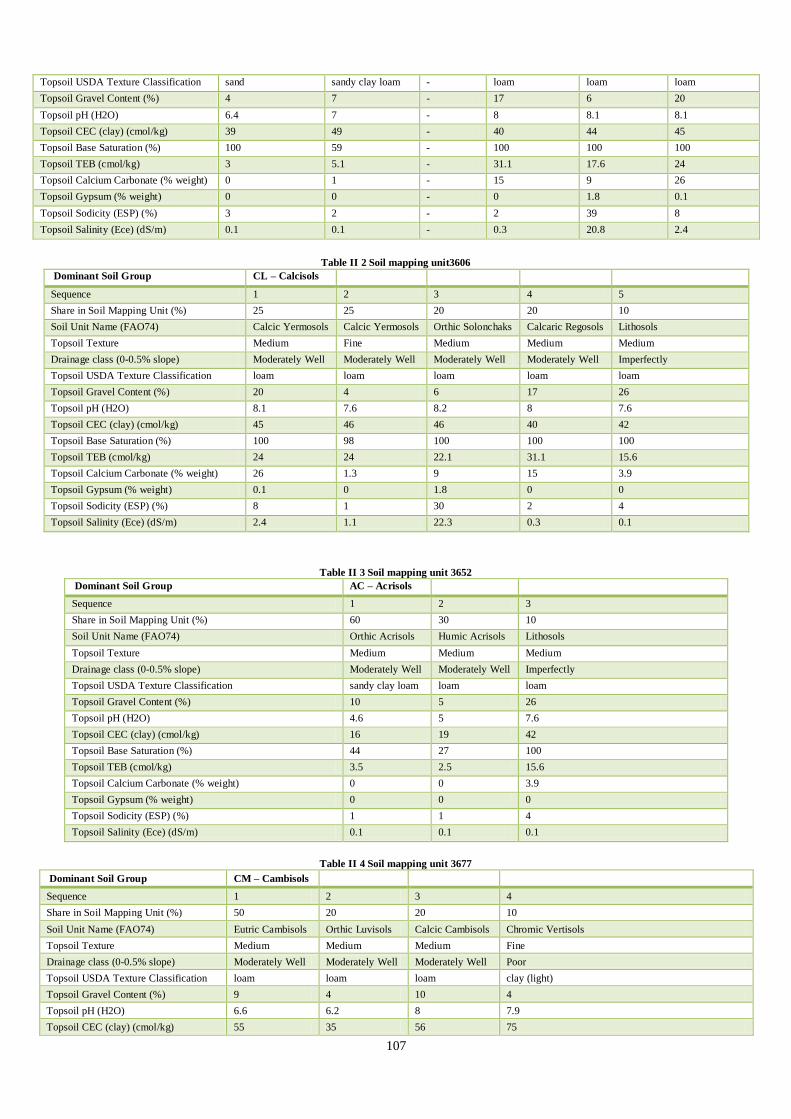
107

Topsoil USDA Texture Classification sand sandy clay loam - loam loam loam

Topsoil Gravel Content (%) 4 7 - 17 6 20

Topsoil pH (H2O) 6.4 7 - 8 8.1 8.1

Topsoil CEC (clay) (cmol/kg) 39 49 - 40 44 45

Topsoil Base Saturation (%) 100 59 - 100 100 100

Topsoil TEB (cmol/kg) 3 5.1 - 31.1 17.6 24

Topsoil Calcium Carbonate (% weight) 0 1 - 15 9 26

Topsoil Gypsum (% weight) 0 0 - 0 1.8 0.1

Topsoil Sodicity (ESP) (%) 3 2 - 2 39 8

Topsoil Salinity (Ece) (dS/m) 0.1 0.1 - 0.3 20.8 2.4

Table II 2 Soil mapping unit3606

Dominant Soil Group CL – Calcisols

Sequence 1 2 3 4 5

Share in Soil Mapping Unit (%) 25 25 20 20 10

Soil Unit Name (FAO74) Calcic Yermosols Calcic Yermosols Orthic Solonchaks Calcaric Regosols Lithosols

Topsoil Texture Medium Fine Medium Medium Medium

Drainage class (0-0.5% slope) Moderately Well Moderately Well Moderately Well Moderately Well Imperfectly

Topsoil USDA Texture Classification loam loam loam loam loam


Topsoil pH (H2O) 8.1 7.6 8.2 8 7.6



Topsoil TEB (cmol/kg) 24 24 22.1 31.1 15.6

Topsoil Calcium Carbonate (% weight) 26 1.3 9 15 3.9

Topsoil Gypsum (% weight) 0.1 0 1.8 0 0


Topsoil Salinity (Ece) (dS/m) 2.4 1.1 22.3 0.3 0.1


Dominant Soil Group AC – Acrisols

Sequence 1 2 3

Share in Soil Mapping Unit (%) 60 30 10

Soil Unit Name (FAO74) Orthic Acrisols Humic Acrisols Lithosols

Topsoil Texture Medium Medium Medium

Drainage class (0-0.5% slope) Moderately Well Moderately Well Imperfectly

Topsoil USDA Texture Classification sandy clay loam loam loam

Topsoil Gravel Content (%) 10 5 26

Topsoil pH (H2O) 4.6 5 7.6

Topsoil CEC (clay) (cmol/kg) 16 19 42

Topsoil Base Saturation (%) 44 27 100

Topsoil TEB (cmol/kg) 3.5 2.5 15.6

Topsoil Calcium Carbonate (% weight) 0 0 3.9

Topsoil Gypsum (% weight) 0 0 0

Topsoil Sodicity (ESP) (%) 1 1 4

Topsoil Salinity (Ece) (dS/m) 0.1 0.1 0.1


Dominant Soil Group CM – Cambisols

Sequence 1 2 3 4

Share in Soil Mapping Unit (%) 50 20 20 10

Soil Unit Name (FAO74) Eutric Cambisols Orthic Luvisols Calcic Cambisols Chromic Vertisols

Topsoil Texture Medium Medium Medium Fine

Drainage class (0-0.5% slope) Moderately Well Moderately Well Moderately Well Poor

Topsoil USDA Texture Classification loam loam loam clay (light)


Topsoil pH (H2O) 6.6 6.2 8 7.9


108


Topsoil TEB (cmol/kg) 13.8 8.3 27.1 45.2


Topsoil Gypsum (% weight) 0 0 0.1 0


Topsoil Salinity (Ece) (dS/m) 0.1 0.1 0.3 0.2



Sequence 1 2 3 4


Soil Unit Name (FAO74) Eutric Cambisols Eutric

Cambisols Orthic Luvisols Vertic Cambisols

Topsoil Texture Medium Fine Medium Fine

Drainage class (0-0.5% slope) Moderately Well Moderately

Well

Moderately

Well Moderately Well

Topsoil USDA Texture Classification loam clay (light) loam clay (light)


Topsoil pH (H2O) 6.6 6.8 6.2 7.1




Topsoil Calcium Carbonate (% weight) 0 0.1 0 0.3






Sequence 1 2 3

Share in soil mapping unit % 60 30 10

Soil Unit Name (FAO74) Eutric Cambisols Orthic Solonchaks Lithosols


PHASE1 Saline - -

Drainage class (0-0.5% slope) Moderately Well Moderately Well Imperfectly

Topsoil USDA Texture Classification loam loam loam


Topsoil pH (H2O) 6.6 8.2 7.6




Topsoil Calcium Carbonate (% weight) 0 9 3.9

Topsoil Gypsum (% weight) 0 1.8 0




Dominant Soil Group LP – Leptosols

Sequence 1 2 3


Database ID 42039 42041 42040

Soil Unit Name (FAO74) Lithosols Chromic Luvisols Chromic Cambisols

Topsoil Texture Medium Medium Fine

Drainage class (0-0.5% slope) Imperfectly Moderately Well Moderately Well

Topsoil USDA Texture Classification loam loam clay (light)


Topsoil pH (H2O) 7.6 6.4 6.8

109



Topsoil TEB (cmol/kg) 15.6 10 20.8

Topsoil Calcium Carbonate (% weight) 3.9 0 0.1






Sequence 1 2 3


Soil Unit Name (FAO74) Lithosols Chromic Luvisols Eutric Cambisols


Drainage class (0-0.5% slope) Imperfectly Moderately Well Moderately Well

Topsoil USDA Texture Classification loam loam loam


Topsoil pH (H2O) 7.6 6.4 6.6




Topsoil Calcium Carbonate (% weight) 3.9 0 0






Sequence 1 2

Share in Soil Mapping Unit (%) 50 50

Soil Unit Name (FAO74) Lithosols Calcaric Regosols

Topsoil Texture Medium Medium

Drainage class (0-0.5% slope) Imperfectly Moderately Well

Topsoil USDA Texture Classification loam loam

Topsoil Gravel Content (%) 26 17

Topsoil pH (H2O) 7.6 8

Topsoil CEC (clay) (cmol/kg) 42 40

Topsoil Base Saturation (%) 100 100

Topsoil TEB (cmol/kg) 15.6 31.1

Topsoil Calcium Carbonate (% weight) 3.9 15

Topsoil Gypsum (% weight) 0 0

Topsoil Sodicity (ESP) (%) 4 2

Topsoil Salinity (Ece) (dS/m) 0.1 0.3


Dominant Soil Group LV – Luvisols

Sequence 1 2 3


Soil Unit Name (FAO74) Chromic Luvisols Chromic Vertisols Lithosols

Topsoil Texture Medium Fine Medium

Drainage class (0-0.5% slope) Moderately Well Poor Imperfectly

Topsoil USDA Texture Classification loam clay (light) loam


Topsoil pH (H2O) 6,4 7,9 7,6



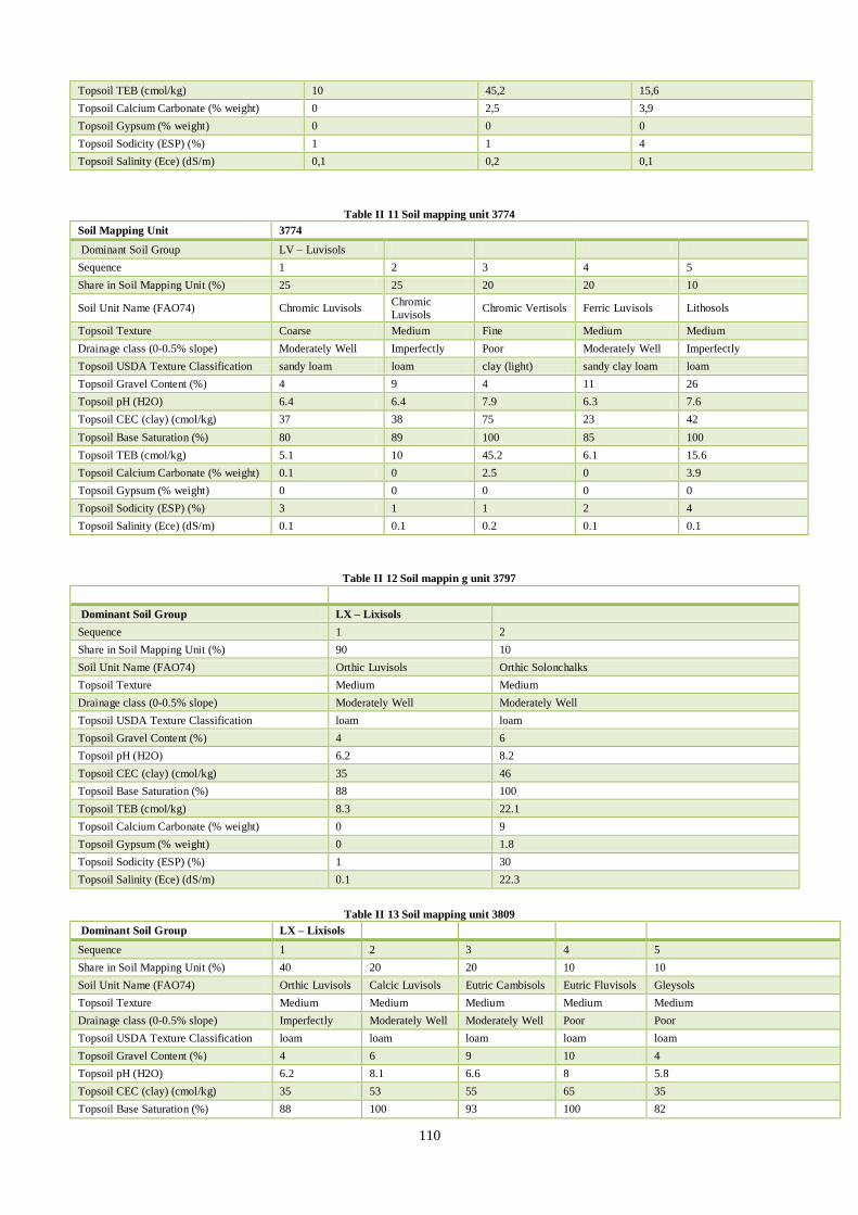
110

Topsoil TEB (cmol/kg) 10 45,2 15,6

Topsoil Calcium Carbonate (% weight) 0 2,5 3,9



Topsoil Salinity (Ece) (dS/m) 0,1 0,2 0,1



Dominant Soil Group LV – Luvisols

Sequence 1 2 3 4 5


Soil Unit Name (FAO74) Chromic Luvisols Chromic

Luvisols Chromic Vertisols Ferric Luvisols Lithosols

Topsoil Texture Coarse Medium Fine Medium Medium

Drainage class (0-0.5% slope) Moderately Well Imperfectly Poor Moderately Well Imperfectly

Topsoil USDA Texture Classification sandy loam loam clay (light) sandy clay loam loam


Topsoil pH (H2O) 6.4 6.4 7.9 6.3 7.6



Topsoil TEB (cmol/kg) 5.1 10 45.2 6.1 15.6

Topsoil Calcium Carbonate (% weight) 0.1 0 2.5 0 3.9

Topsoil Gypsum (% weight) 0 0 0 0 0



Table II 12 Soil mappin g unit 3797

Dominant Soil Group LX – Lixisols

Sequence 1 2


Soil Unit Name (FAO74) Orthic Luvisols Orthic Solonchalks


Drainage class (0-0.5% slope) Moderately Well Moderately Well



Topsoil pH (H2O) 6.2 8.2




Topsoil Calcium Carbonate (% weight) 0 9

Topsoil Gypsum (% weight) 0 1.8




Dominant Soil Group LX – Lixisols

Sequence 1 2 3 4 5


Soil Unit Name (FAO74) Orthic Luvisols Calcic Luvisols Eutric Cambisols Eutric Fluvisols Gleysols

Topsoil Texture Medium Medium Medium Medium Medium

Drainage class (0-0.5% slope) Imperfectly Moderately Well Moderately Well Poor Poor

Topsoil USDA Texture Classification loam loam loam loam loam


Topsoil pH (H2O) 6.2 8.1 6.6 8 5.8



111

Topsoil TEB (cmol/kg) 8.3 18.9 13.8 19.8 8.8

Topsoil Calcium Carbonate (% weight) 0 10.8 0 11.7 0

Topsoil Gypsum (% weight) 0 0 0 0.2 0




Dominant Soil Group AR – Arenosols

Sequence 1 2


Soil Unit Name (FAO74) Cambic Arenosols Calcaric Regosols

Topsoil Texture Coarse Medium

Drainage class (0-0.5% slope) Somewhat Excessive Moderately Well

Topsoil USDA Texture Classification sand loam


Topsoil pH (H2O) 6.4 8



Topsoil TEB (cmol/kg) 3 31.1

Topsoil Calcium Carbonate (% weight) 0 15

Topsoil Gypsum (% weight) 0 0




Dominant Soil Group AR – Arenosols

Sequence 1 2 3 4 5


Soil Unit Name (FAO74) Cambic Arenosols Haplic Xerosols Orthic Solonchaks Calcic Xerosols Eutric Fluvisols

Topsoil Texture Coarse Medium Medium Medium Medium

Drainage class (0-0.5% slope) Somewhat Excessive Moderately Well Moderately Well Moderately Well Poor

Topsoil USDA Texture Classification sand loam loam loam loam


Topsoil pH (H2O) 6.4 8.2 8.2 7.9 8



Topsoil TEB (cmol/kg) 3 14.3 22.1 33.2 19.8

Topsoil Calcium Carbonate (% weight) 0 14.5 9 9 11.7

Topsoil Gypsum (% weight) 0 0 1.8 0.4 0.2




Dominant Soil Group VR – Vertisols

Sequence 1 2 3


Soil Unit Name (FAO74) Chromic Vertisols Chromic Vertisols Vertic Cambisols

Topsoil Texture Medium Fine Fine

Drainage class (0-0.5% slope) Poor Poor Moderately Well

Topsoil USDA Texture Classification sandy clay loam clay (light) clay (light)


Topsoil pH (H2O) 6.8 7.9 7.1


112



Topsoil Calcium Carbonate (% weight) 0.3 2.5 0.3






Sequence 1 2 3


Soil Unit Name (FAO74) Chromic Vertisols Chromic Luvisols Chromic Cambisols

Topsoil Texture Fine Medium Fine

Drainage class (0-0.5% slope) Poor Moderately Well Moderately Well

Topsoil USDA Texture Classification clay (light) loam clay (light)


Topsoil pH (H2O) 7.9 6.4 6.8




Topsoil Calcium Carbonate (% weight) 2.5 0 0.1






Sequence 1 2 3


Soil Unit Name (FAO74) Chromic Vertisols Vertic Cambisols Lithosols

Topsoil Texture Fine Fine Medium

Drainage class (0-0.5% slope) Poor Moderately Well Imperfectly

Topsoil USDA Texture Classification clay (light) clay (light) loam


Topsoil pH (H2O) 7.9 7.1 7.6




Topsoil Calcium Carbonate (% weight) 2.5 0.3 3.9





Sequence 1 2 3


Soil Unit Name (FAO74) Haplic

Yermosols

Haplic

Yermosols Orthic Solonchaks

Topsoil Texture Medium Fine Medium

PHASE1 Saline Saline -

Drainage class (0-0.5% slope) Moderately Well Moderately Well Moderately Well

Topsoil USDA Texture Classification loam clay (light) loam


Topsoil pH (H2O) 8.3 7.7 8.2

113




Topsoil Calcium Carbonate (% weight) 1.5 3 9

Topsoil Gypsum (% weight) 0.1 0 1.8


Topsoil Salinity (Ece) (dS/m) 1 1.1 22.3


Sequence 1 2 3 4


Soil Unit Name (FAO74) Calcic Yermosols Cambic Arenosols Orthic Solonchaks Calcaric Regosols

Topsoil Texture Fine Coarse Medium Medium

Drainage class (0-0.5% slope) Moderately Well Somewhat Excessive Moderately Well Moderately Well

Topsoil USDA Texture Classification loam sand loam loam


Topsoil pH (H2O) 7,6 6,4 8,2 8



Topsoil TEB (cmol/kg) 24 3 22,1 31,1

Topsoil Calcium Carbonate (% weight) 1,3 0 9 15

Topsoil Gypsum (% weight) 0 0 1,8 0


Topsoil Salinity (Ece) (dS/m) 1,1 0,1 22,3 0,3


Sequence 1 2 3 4



Topsoil Texture Medium Medium Medium Medium

Drainage class (0-0.5% slope) Moderately Well Moderately Well Moderately Well Moderately Well

Topsoil USDA Texture Classification loam loam loam loam


Topsoil pH (H2O) 8.1 8 8.2 7.9



Topsoil TEB (cmol/kg) 24 31.1 22.1 10.4


Topsoil Gypsum (% weight) 0.1 0 1.8 15.1





Dominant Soil Group SC – Solonchaks

Sequence 1 2 3 4


Soil Unit Name (FAO74) Orthic Solonchaks Haplic Yermosols Calcaric Regosols Eutric Fluvisols

Topsoil Texture Fine Medium Medium Medium

Drainage class (0-0.5% slope) Moderately Well Moderately Well Moderately Well Poor

Topsoil USDA Texture Classification clay (light) loam loam loam


Topsoil pH (H2O) 8.3 8.3 8 8


114



Topsoil Calcium Carbonate (% weight) 10.6 1.5 15 11.7

Topsoil Gypsum (% weight) 1.3 0.1 0 0.2


Topsoil Salinity (Ece) (dS/m) 5.9 1 0.3 0.7


Dominant Soil Group CL – Calcisols

Sequence 1 2


Soil Unit Name (FAO74) Haplic Xerosols Calcic Xerosols


PHASE1 Saline -

Drainage class (0-0.5% slope) Moderately Well Moderately Well



Topsoil pH (H2O) 8.2 7.9




Topsoil Calcium Carbonate (% weight) 14.5 9

Topsoil Gypsum (% weight) 0 0.4



10.3 Appendix III Soil mapping unit of Rajasthan district-wise

Table III 1 Soil mapping unit of Rajasthan district-wise

District Soil mapping unit District Soil mapping unit

Ajmer 3677; 3678; 3840; 6673 Jaipur 3541; 3677; 3716; 3840; 3878

Alwar 3716; 3797; 3840; 3878 Jaisalmer 3541; 3606; 3730; 3839; 3882

Banswara 3652; 3858; 3859 Jalore 3541; 6673

Baran 3686; 3714; 3781; 3861 Jhalawar 3861

Barmer 3541; 3716; 3730; 6673 Jhunjhunu 3541; 3716; 3840

Bharatpur 3686; 3797; 3714 Jodhpur 3541; 6673

Bhilwara 3677; 3678; 3809 Karauli 3677; 3686; 3714; 3716

Bikaner 3541; 3882 Kota 3714; 3809; 3861

Bundi 3677; 3714; 3809; 3861 Nagaur 3541; 3716; 3840; 6673

115

Chittaurgarh 3677; 3809; 3859; 3861 Pali 3716; 3677; 6673

Churu 3541 Rajsamand 3677; 3716

Dausa 3677 Sawai madhopur 3677; 3686; 3714; 3716; 3861

Dholpur 3686; 3714 Sikar 3541; 3716; 3840

Dungarpur 3774; 3858; 3859 Sirohi 3616; 6673

Ganganagar 3541; 3878; 3880; 3891 Tonk 3677; 3678

Hanumangarh 3541; 3878; 3891 Udaipur 3677; 3678; 3716; 3840; 6673

10.4 Appendix IV Slope

Table IV 1 Slope and slope rating district-wise

Districts Nearly level

(0-1%) %

Very gently sloping

(1-3%) %

Gently sloping

(3-8%) %

Moderatly sloping (8-

15%) %

Steeply sloped

(>30%) % Rating

Ajmer 68 0 27 0 5 94

Alwar 42 0 36 22 0 90

Barmer 7 0 81 11 1 88

Banswara 21 0 62 13 4 88

Baran 56 0 8 1 36 75

Bharatpur 56 0 38 0 7 92

Bhilwara 68 0 25 0 7 93

Bikaner 46 0 30 22 3 89

116

Bundi 38 0 46 0 17 84

Chittaurgarh 37 0 29 1 33 74

Churu 7 0 86 6 0 90

Dausa 71 0 20 0 8 92

Dholpur 48 0 31 0 21 83

Dungarpur 0 0 70 0 30 73

Ganganagar 33 0 65 2 0 93

Hanumangarh 34 0 56 10 0 92

Jalore 35 0 61 0 4 91

Jaipur 47 0 45 0 8 90

Jaisalmer 19 0 43 36 3 84

Jhalawar 66 0 13 0 21 84

Jhunjhunu 6 0 84 0 10 85

Jodhpur 38 0 61 1 0 93

Karauli 57 0 29 0 14 88

Kota 64 0 13 0 23 83

Nagaur 9 0 91 0 0 91

Pali 67 0 27 0 6 93

Rajsamand 42 0 25 3 31 76

Sikar 21 0 72 0 7 88

Sirohi 32 0 35 0 33 74

Sawai madhopur 26 0 41 0 33 74

Tonk 25 0 72 0 3 91

Udaipur 8 0 39 1 52 61

10.5 Appendix V Climate characteristics

Table V 1 Climate characteristics and climate rating

Rating

Annual

rain

Dry

season

T-

max

T-

mean

T-

min

Sun

Fr

Annual

rain

Dry

season

T-

max

T-

mean

T-

min

Sun

Fr

Ajmer 751 9 31.13 25.68 18.25 0.65 90 50 90 100 90 90

Alwar 801 9 34.4 26.3 18.2 0.67 90 50 90 100 90 90

Barmer 311 11 32.2 25.7 19.1 0.47 50 13 90 100 90 73

Banswara 1032 9 32.2 25.7 19.1 0.47 90 50 90 100 90 73

Baran 707 9 34 27.7 22 0.71 73 50 73 100 100 100

Bharatpur 641 9 28.2 20.2 12.3 0.48 73 50 100 100 73 73

Bhilwara 848 9 32.5 27.1 18.6 0.52 90 50 90 100 90 90

117

Bikaner 301 12 36.2 27.7 19.1 0.66 50 13 73 100 90 90

Bundi 803 9 34.5 27.3 21 0.59 90 50 73 100 100 90

Chittaurgarh 848 9 32.5 27.1 18.6 0.52 90 50 90 100 90 90

Churu 480 11 33 25.1 17.1 0.71 50 13 90 100 90 100

Dausa 609 10 34.4 26.3 18.2 0.67 73 33 73 100 90 90

Dholpur 811 9 34.2 26.7 19.8 0.48 90 50 73 100 90 73

Dungarpur 1498 7 31.3 27.2 22.2 0.42 100 73 90 100 100 73

Ganganagar 237 12 35 26 17 0.75 33 13 73 100 90 100

Hanumangarh 237 12 35 26 17 0.75 33 13 73 100 90 100

Jaipur 609 10 34.4 26.3 18.2 0.67 73 33 73 100 90 90

Jaisalmer 216 11 36 28.1 20.1 0.88 33 13 73 100 100 100

Jalore 393 9 26.6 22 17.3 0.55 50 50 100 100 90 90

Jhalawar 903 9 33.5 27.2 18.2 0.6 90 50 90 100 90 90

Jhunjhunu 402 10 33 25.1 17.1 0.71 50 33 90 100 90 100

Jodhpur 402 10 35.7 27.7 19.6 0.62 50 33 73 100 90 90

Karauli 811 9 32.9 25.6 18.3 0.73 90 50 90 100 90 100

Kota 1410 7 28.5 24.3 18.3 0.44 100 73 100 100 90 73

Nagaur 281 11 36.2 27.7 19.1 0.66 33 13 73 100 90 90

Pali 1258 8 30.6 25.7 17.6 0.38 100 50 90 100 90 73

Rajsamand 705 7 32 25.3 18.8 0.63 73 73 90 100 90 90

Sikar 441 10 33 25.1 17.1 0.71 50 33 90 100 90 100

Sirohi 1691 8 26.6 22 17.3 0.55 100 50 100 100 90 90

Sawai

madhopur 861 9 32.9 25.6 18.3 0.73 90 50 90 100 90 100

Tonk 623 9 33.2 25.5 18.2 0.47 73 50 90 100 90 73

Udaipur 674 8 32 25.3 18.8 0.63 73 50 90 100 90 90

Table IV 2 District-wise agro-climatic zone. groundwater level and constrains for plantation

District Agro-climatic zone Average altitude m Ground water level Constrains

Ajmer IIIA-Semi-Arid Eastern Plain 471 5-20

Alwar IIIB-Flood Prone Eastern Plain 250 <5-15<

Barmer IA-Arid Western 227 10-40< Frost. water level

Banswara IVB-Humid southern 243 2-9

Baran V-Humid Southern Eastern Plain 265 <10-20

Bharatpur IIIB-Flood Prone Eastern Plain 250 5-20

Bhilwara IVA-Sub humid Southern Plain 432 5-20

Bikaner IC-Hyper Arid Partial Irrigated Zone 246 40-120 water level

118

Bundi V-Humid Southern Eastern Plain 268 12-18

Chittaurgarh IVA-Sub humid Southern Plain 392 <10-20<

Churu IC-Hyper Arid Partial Irrigated Zone 321 <40-80<

Dausa IIIA-Semi-Arid Eastern Plain 381 <10-20

Dholpur IIIB-Flood Prone Eastern Plain 177 0-15

Dungarpur IVB-Humid southern 225 5-10

Ganganagar IB-Irrigated North Western Plain 176 20-40< High speed wind

Hanumangarh IB-Irrigated North Western Plain 177 10-20

Jalore IIB-Transitional Plain of Luni Basin 222 10-40<

Jaipur IIIA-Semi-Arid Eastern Plain 431 <10-40<

Jaisalmer IC-Hyper Arid Partial Irrigated Zone 264 40-120 Frost. watr level

Jhalawar V-Humid Southern Eastern Plain 312 <8-14

Jhunjhunu IIA-Internal Drainage dry zone 323 30-80

Jodhpur IA-Arid Western 269 20-40 Water level

Karauli IIIB-Flood Prone Eastern Plain 275 10-20

Kota V-Humid Southern Eastern Plain 271 6-16

Nagaur IIA-Internal Drainage dry zone 302 20-40

Pali IIB-Transitional Plain of Luni Basin 214 10-20

Rajsamand IVA-Sub humid Southern Plain 533 10-20

Sikar IIA-Internal Drainage dry zone 341 20-60

Sirohi IIB-Transitional Plain of Luni Basin 320 <10-40<

Sawai madhopur IIIB-Flood Prone Eastern Plain 350 10-20

Tonk IIIA-Semi-Arid Eastern Plain 289 5-10

Udaipur IVB-Humid southern 582 15-25

10.6 Appendix VI District-wise pre-monsoon groundwater level maps

119

Figure VI 1 Ajmer (2006)

Figure VI 2 Alwar (2006)

Figure VI 3 Banswara (2007)

120

Figure VI 4 Barmer (2006)

Figure VI 5 Bharatpur (2007)

Figure VI 6 Baran (2006)

121

Figure VI 7 Bhilwara (2006)

Figure VI 8 Bikaner (2006)

Figure VI 9 Bundi (2006)

122

Figure VI 10 Churu (2006)

Figure VI 11 Chittaurgarh (2006)

Figure VI 12 Dausa (2006)

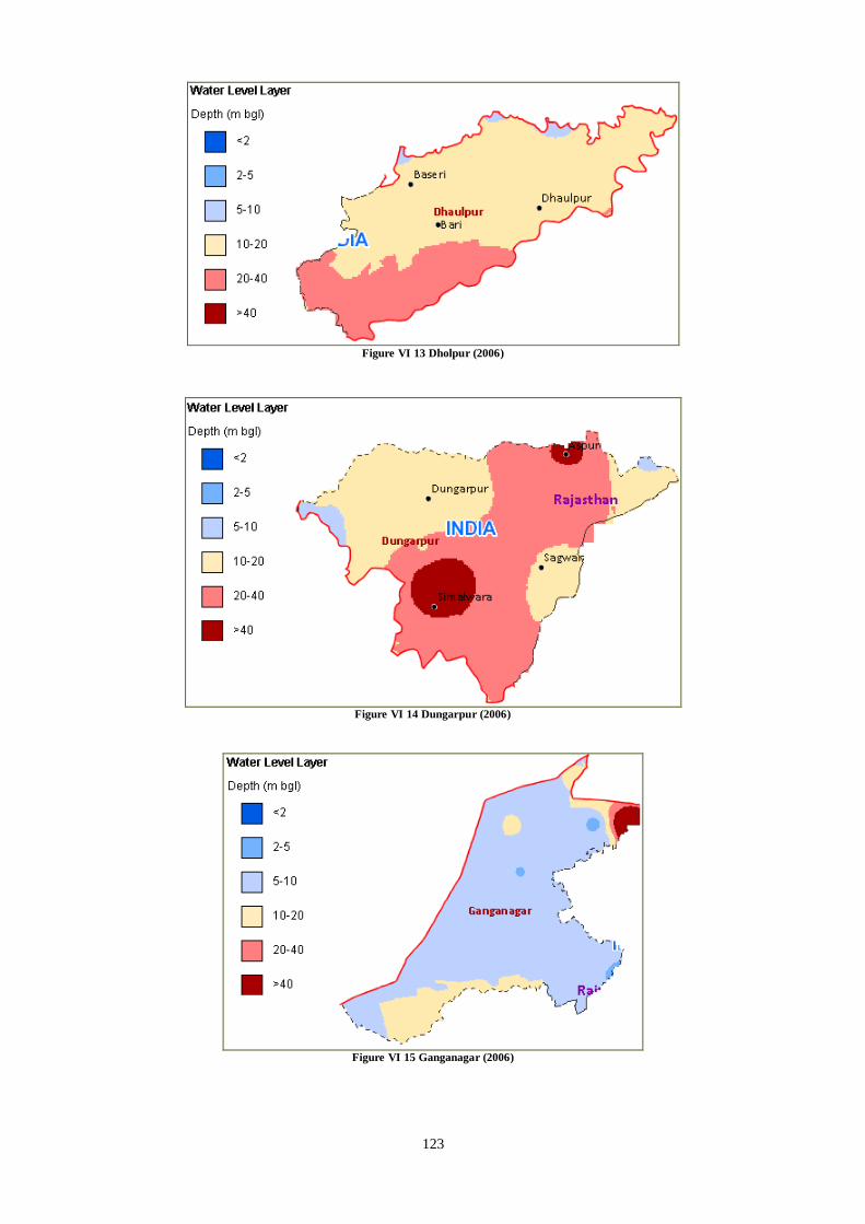
123

Figure VI 13 Dholpur (2006)

Figure VI 14 Dungarpur (2006)

Figure VI 15 Ganganagar (2006)

124

Figure VI 16 Hanumangarh (2006)

Figure VI 17 Jaipur (2006)

Figure VI 18 Jalore (2006)

125

Figure VI 19 Jaisalmer (2006)

Figure VI 20 Jhalawar (2008)

126

Figure VI 21 Jhunjhunu (2007)

Figure VI 22 Jodhpur (2006)

127

Figure VI 23 Karauli (2006)

Figure VI 24 Kota (2006)

Figure VI 25 Nagaur (2006)

128

Figure VI 26 Pali (2006)

Figure VI 27 Rajsamand (2006)

Figure VI 28 Sikar (2006)

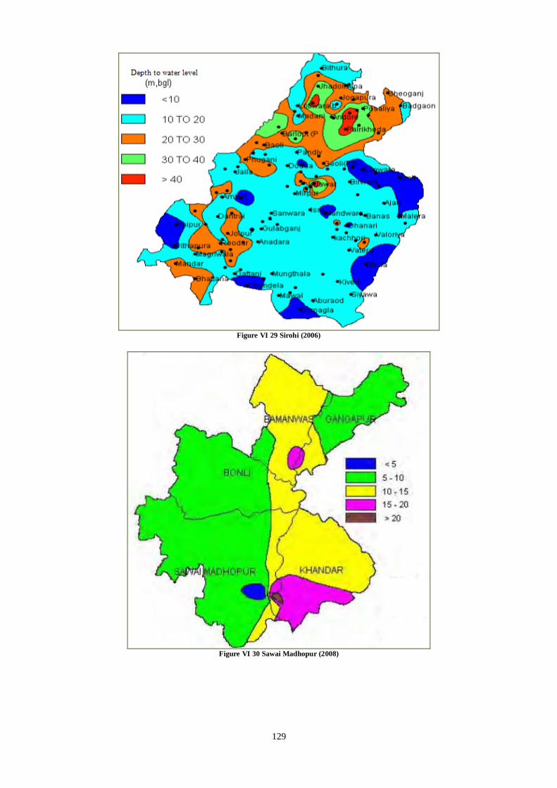
129

Figure VI 29 Sirohi (2006)

Figure VI 30 Sawai Madhopur (2008)

130

Figure VI 31 Tonk (2006)

Figure VI 32 Udaipur (2006)

131

10.7 Appendix VII Nursery raising costs

Table VII 1 Cost of Nursery raising

Fixed Cost Required Unit Price Unit Cost (Rs.)

Site Preparation 13 MD 147 Rs./MD 1882

Fencing with barbed wire 240 RMT 48 Rs/RMT 11531

Preparation of compost pit. nursery path 10 MD 147 Rs./MD 1470

Maintenance of irrigation source 3203 LS 3203

5 HP Diesel Pumpset 40039 LS 40039

Cost of pipeline for irrigation 160 M 24 Rs./M 3844

Cost of implements for nursery operations 4004 LS 2500

Cost of Water Tank 8008 LS 8008

Preparation of Polybeds 20 MD 147 Rs./MD 2917

Cost of Net for providing shade and installation 76874 LS 76874

SubTotal 152267

Contingency 5% 7613

Total 159880

Recurring Cost

Rent for land 0 ha 16015 Rs/ha 6406

Cost of seeds 2 kg 801 Rs./kg 1602

Cost of Polybags 125 kg 64 Rs./kg 8008

Cost of Pot mixture including loading. unloading 50 tonnes 192 Rs/MT 9609

Cost of diesel and lubricants for pumpsets 1 ltr/hr 49 Rs./ltr 7350

Cost of thatching material 1602 LS 1602

Cost of weeding and hoeing 20 MD 147 Rs./MD 2940

Filling up of polybags 250 MD 147 Rs./MD 36750

Shifting of polybags 21 MD 147 Rs./MD 3063

Cost of labour for irrigation 40 MD 147 Rs./MD 5880

Maintenance of paths 10 MD 157 Rs./MD 1570

Maintenance of pumpset 167 LS 167

Watch and ward 5 months 1602 Rs./month 8008

Subtotal 92953

Cost of supervision 5% 4648

Total 97601

Grand Total 257481

Cost per seedling Rs./seedling 5.1

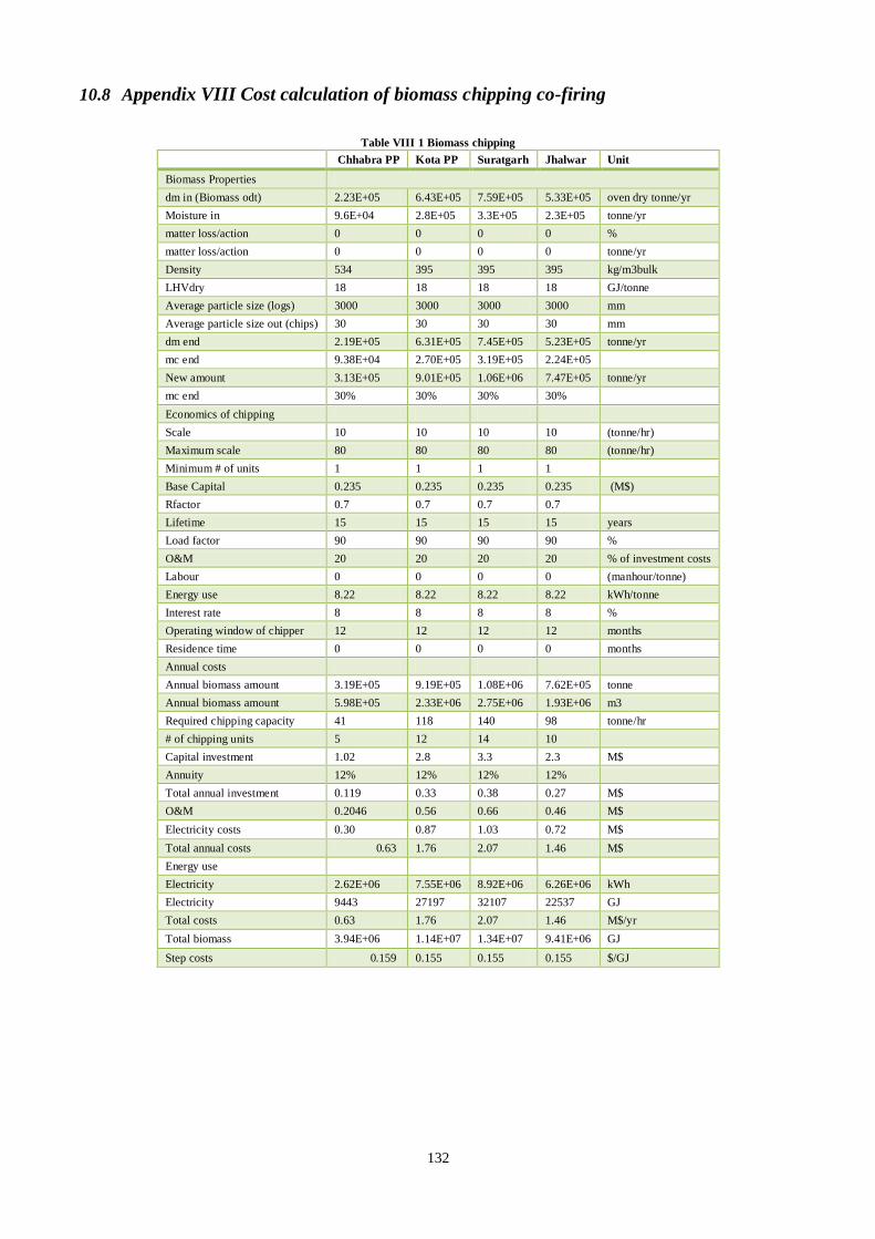
132

10.8 Appendix VIII Cost calculation of biomass chipping co-firing

Table VIII 1 Biomass chipping

Chhabra PP Kota PP Suratgarh Jhalwar Unit

Biomass Properties

dm in (Biomass odt) 2.23E+05 6.43E+05 7.59E+05 5.33E+05 oven dry tonne/yr

Moisture in 9.6E+04 2.8E+05 3.3E+05 2.3E+05 tonne/yr

matter loss/action 0 0 0 0 %

matter loss/action 0 0 0 0 tonne/yr

Density 534 395 395 395 kg/m3bulk

LHVdry 18 18 18 18 GJ/tonne

Average particle size (logs) 3000 3000 3000 3000 mm

Average particle size out (chips) 30 30 30 30 mm

dm end 2.19E+05 6.31E+05 7.45E+05 5.23E+05 tonne/yr

mc end 9.38E+04 2.70E+05 3.19E+05 2.24E+05

New amount 3.13E+05 9.01E+05 1.06E+06 7.47E+05 tonne/yr

mc end 30% 30% 30% 30%

Economics of chipping

Scale 10 10 10 10 (tonne/hr)

Maximum scale 80 80 80 80 (tonne/hr)

Minimum # of units 1 1 1 1

Base Capital 0.235 0.235 0.235 0.235 (M$)

Rfactor 0.7 0.7 0.7 0.7

Lifetime 15 15 15 15 years

Load factor 90 90 90 90 %

O&M 20 20 20 20 % of investment costs

Labour 0 0 0 0 (manhour/tonne)

Energy use 8.22 8.22 8.22 8.22 kWh/tonne

Interest rate 8 8 8 8 %

Operating window of chipper 12 12 12 12 months

Residence time 0 0 0 0 months

Annual costs

Annual biomass amount 3.19E+05 9.19E+05 1.08E+06 7.62E+05 tonne

Annual biomass amount 5.98E+05 2.33E+06 2.75E+06 1.93E+06 m3

Required chipping capacity 41 118 140 98 tonne/hr

# of chipping units 5 12 14 10

Capital investment 1.02 2.8 3.3 2.3 M$

Annuity 12% 12% 12% 12%

Total annual investment 0.119 0.33 0.38 0.27 M$

O&M 0.2046 0.56 0.66 0.46 M$

Electricity costs 0.30 0.87 1.03 0.72 M$

Total annual costs 0.63 1.76 2.07 1.46 M$

Energy use

Electricity 2.62E+06 7.55E+06 8.92E+06 6.26E+06 kWh

Electricity 9443 27197 32107 22537 GJ

Total costs 0.63 1.76 2.07 1.46 M$/yr

Total biomass 3.94E+06 1.14E+07 1.34E+07 9.41E+06 GJ

Step costs 0.159 0.155 0.155 0.155 $/GJ

133

10.9 Appendix IX Cost calculation of biomass drying (co-firing)

Table IX 1 Biomass drying


Biomass Properties

Dry matter input biomass 2.10E+05 6.50E+05 7.67E+05 5.39E+05 Tonne/year

Moisture in 8.98E+04 2.79E+05 3.29E+05 2.31E+05 Tonne/year

LHV (GJ/oven dry) 18 18 18 18 GJ/tonne

Average particle size 30 30 30 30 mm


matter loss/action 0 0 0 0 Tonne/year

mc loss (forced) 66784 207101 244494 171621 Tonnes/year

dry matter combusted 9276 28764 33958 23836 Tonnes/year

Biomass combusted (mc30% ) 13251 41091 48511 34052 Tonne/year

mc end (forced) 10 10 10 10 %

mc end (forced) 2.31E+04 7.15E+04 8.44E+04 5.93E+04 Tonnes/year

dm end 2.08E+05 6.44E+05 7.60E+05 5.33E+05 Tonnes/year

New amount 2.31E+05 7.15E+05 8.44E+05 5.93E+05 Tonnes/year

Economics of drying

Scale of dryer (rotary drum type) 100 100 1.00E+02 100 Tonne/hour

Base Capital dryer 8.39 8.39 8.39 8.39 (M$

Rfactor 0.7 0.7 0.7 0.7


Load factor 100 100 100 100 %

O&M 3% 0.03 0.03 0.03 % of investment costs

Energy use (electricity) 20 20 20 20 kWh/tonne

Energy use (heat) 2.5 2.5 2.5 2.5 GJ/tonne water evap.


Operating window of dryer 12 12 12 12 Months

Annual costs

Annual biomass amount 2.99E+05 9.29E+05 1.10E+06 7.70E+05 Tonne

Required drying capacity 35 107 127 89 Tonne/hour

# of dryer units 1 2 2 1


Annuity 12% 12% 12% 12%


O&M 0.120 0.326 0.366 0.232 M$



Energy use


Electricity 2.16E+04 6.69E+04 7.89E+04 5.54E+04 GJ

Heat GJ/year

Total costs 1.28 3.7 4.3 2.9 M$/year


Step costs 0.34 0.32 0.32 0.30 $/GJ

6.17 5.82 5.70 5.47 $/oven dry tonne

134

10.10 Appendix X Cost calculation of biomass sizing (co-firing)

Table X 1 Biomass sizing (Hammer-mill)


Biomass Properties

Dry matter input (mc 10%) 2.31E+05 7.15E+05 8.44E+05 5.93E+05 Tonne/year

Moisture content 10 10 10 10 %

dm in 2.08E+05 6.44E+05 7.60E+05 5.33E+05 Tonne/year

Moisture in 2.31E+04 7.15E+04 8.44E+04 5.93E+04 Tonne/year


LHVdry 18 18 18 18 GJ/tonne

Average particle size 30 30 30 30 mm

matter loss/action 0 0 0 0

matter loss/action 0 0 0 0 Tonne/year

Average particle size out 10 10 10 10 mm

dm end 2.03E+05 6.31E+05 7.45E+05 5.23E+05 Tonne/year

mc end 10% 10% 10% 10%

moist end 2.26E+04 7.01E+04 8.27E+04 5.81E+04 Tonne/year

New amount 2.26E+05 7.01E+05 8.27E+05 5.81E+05 Tonne/year

Economics of grinding

Scale of hammer mill 50 50 50 50 Tonne/hour

Base Capital of hammermill 0.621 0.621 0.621 0.621 M$

Rfactor 0.7 0.7 0.7 0.7




Energy use 3.5 3.5 3.5 3.5 kWh/tonne


Operating window of hammer mill 12 12 12 12 Months

Residence time 0 0 0 0 Months

Annual costs

Annual biomass amount 2.31E+05 7.15E+05 8.44E+05 5.93E+05 Tonne

Annual biomass amount 5.40E+05 1.67E+06 1.98E+06 1.39E+06 m3

Required grinding capacity 30 92 109 76 Tonne/hour

# of hammer mills units 1 2 3 2


Annuity 12 12 12 12 %


O&M 0.09 0.234 0.297 0.205 M$



Energy use





Step costs 0.06 0.058 0.061 0.060 $/GJ

135

10.11 Appendix XI Cost calculation of biomass pelletizing (co-firing)

Table XI 1 Pelletizing of biomass

Chhabra PP Kota PP Suratgarh Jhalawar Unit

Biomass properties

Biomass input (mc 10%) 2.26E+05 7.01E+05 8.27E+05 5.81E+05 tonne/year

Moisture content 10 10 10 10 %

Moisture in 2.26E+04 7.01E+04 8.27E+04 5.81E+04 tonne/year

dm in 2.03E+05 6.31E+05 7.45E+05 5.23E+05


LHVdry (odt) 18 18 18 18 GJ/tonne


matter loss/action 0 0 0 0 tonne/year

Average particle size out 10 10 10 10 mm

Product characteristics

Form Pellets Pellets Pellets Pellets

Bulk density 650 620 620 620 kg/m3bulk

LHV (oven dry) 11 10 10 10 GJ/m3

dm end 2.03E+05 6.31E+05 7.45E+05 5.23E+05 tonne/year

mc end 10 10 10 10 %

moist end 2.26E+04 7.01E+04 8.27E+04 5.81E+04 tonne/year

New amount 2.26E+05 7.01E+05 8.27E+05 5.81E+05 tonne/year

Economics of pelletizing

Scale of pellet mill 6 6 6 6 (tonne/hour)

Base Capital of pellet mill 0.201 0.201 0.201 0.201 (M$)

Rfactor 0.61 0.61 0.61 0.61




Energy use 28 28 28 28 kWhe/tonne


Operating window 12 12 12 12 months

Residence time 0 0 0 0 months

Annual costs

Annual biomass amount 2.26E+05 7.01E+05 8.27E+05 5.81E+05 tonne/year

Required pelletising capacity 29 90 106 75 tonne/hour

# of pellet mills units 5 16 18 13


Annuity 15 15 15 15 %


O&M 1.95 6.11 7.07 5.02 M$



Energy use





Step costs 0.77 0.779 0.768 0.774 $/GJ

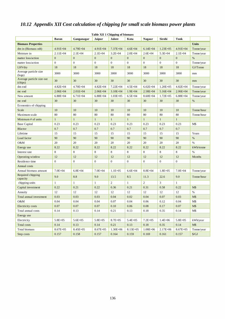
136

10.12 Appendix XII Cost calculation of chipping for small scale biomass power plants

Table XII 1 Chipping of biomass

Baran Ganganagar Jaipur Jalore Kota Nagaur Sirohi Tonk

Biomass Properties Units

dm in (Biomass odt) 4.91E+04 4.79E+04 4.91E+04 7.37E+04 4.6E+04 6.14E+04 1.23E+05 4.91E+04 Tonne/year

Moisture in 2.11E+04 2.1E+04 2.1E+04 3.2E+04 2.0E+04 2.6E+04 5.3E+04 2.1E+04 Tonne/year

matter loss/action 0 0 0 0 0 0 0 0 %

matter loss/action 0 0 0 0 0 0 0 0 Tonne/year

LHVdry 18 18 18 18 18 18 18 18 GJ/Tonne

Average particle size

(logs) 3000 3000 3000 3000 3000 3000 3000 3000 mm

Average particle size out

(chips) 30 30 30 30 30 30 30 30 mm

dm end 4.82E+04 4.70E+04 4.82E+04 7.22E+04 4.5E+04 6.02E+04 1.20E+05 4.82E+04 Tonne/year

mc end 2.06E+04 2.01E+04 2.06E+04 3.10E+04 1.9E+04 2.58E+04 5.16E+04 2.06E+04 Tonne/year

New amount 6.88E+04 6.71E+04 6.88E+04 1.03E+05 6.5E+04 8.60E+04 1.72E+05 6.88E+04 Tonne/year

mc end 30 30 30 30 30 30 30 30 %

Economics of chipping

Scale 10 10 10 10 10 10 10 10 Tonne/hour

Maximum scale 80 80 80 80 80 80 80 80 Tonne/hour

Minimum # of units 1 1 1 1 1 1 1 1

Base Capital 0.23 0.23 0.23 0.23 0.23 0.23 0.23 0.23 M$

Rfactor 0.7 0.7 0.7 0.7 0.7 0.7 0.7 0.7

Lifetime 15 15 15 15 15 15 15 15 Years

Load factor 90 90 90 90 90 90 90 90 %

O&M 20 20 20 20 20 20 20 20 %

Energy use 8.22 8.22 8.22 8.22 8.22 8.22 8.22 8.22 kWh/tonne

Interest rate 8 8 8 8 8 8 8 8 %

Operating window 12 12 12 12 12 12 12 12 Months

Residence time 0 0 0 0 0 0 0 0

Annual costs

Annual biomass amount 7.0E+04 6.8E+04 7.0E+04 1.1E+05 6.6E+04 8.8E+04 1.8E+05 7.0E+04 Tonne/year

Required chipping

capacity 9.0 8.8 9.0 13.5 8.5 11.3 22.6 9.0 Tonne/hour

chipping units 1 1 1 2 1 2 3 1

Capital investment 0.22 0.21 0.22 0.36 0.21 0.31 0.58 0.22 M$

Annuity 12 12 12 12 12 12 12 12 %

Total annual investment 0.03 0.03 0.03 0.04 0.02 0.04 0.07 0.03 M$

O&M 0.04 0.04 0.04 0.07 0.04 0.06 0.12 0.04 M$

Electricity costs 0.07 0.07 0.07 0.10 0.06 0.08 0.17 0.07 M$

Total annual costs 0.14 0.13 0.14 0.21 0.13 0.18 0.35 0.14 M$

Energy use

Electricity 5.8E+05 5.6E+05 5.8E+05 8.7E+05 5.4E+05 7.2E+05 1.4E+06 5.8E+05 kWh/year

Total costs 0.14 0.13 0.14 0.21 0.13 0.18 0.35 0.14 M$

Total biomass 8.67E+05 8.45E+05 8.67E+05 1.30E+06 8.13E+05 1.08E+06 2.17E+06 8.67E+05 Tonne/year

Step costs 0.157 0.158 0.157 0.164 0.159 0.169 0.161 0.157 $/GJ

137

10.13 Appendix XIII Cost calculation of drying for small scale biomass power plants

Table XIII 1 Drying of biomass

Baran Ganganagar Jaipur Jalor Kota Nagaur Sirohi Tonk

Biomass properties Unit

Biomass input comb inc (mc 30%) 7E+04 7E+04 7E+04 1E+05 6E+04 9E+04 2E+05 7E+04 Tonnes/year

Biomass input (mc 30%) 7E+04 6E+04 7E+04 1E+05 6E+04 8E+04 2E+05 7E+04 Tonnes/year

Dry matter input biomass 5E+04 4E+04 5E+04 7E+04 4E+04 6E+04 1E+05 5E+04 Tonnes/year

Moisture in 2E+04 2E+04 2E+04 3E+04 2E+04 2E+04 5E+04 2E+04 Tonnes/year

LHVdry 2E+01 2E+01 2E+01 2E+01 2E+01 2E+01 2E+01 2E+01 GJ/Tonne

Average particle size 3E+01 3E+01 3E+01 3E+01 3E+01 3E+01 3E+01 3E+01 mm


matter loss/action 0 0 0 0 0 0 0 0 Tonnes/year

mc loss (forced) 1E+04 1E+04 1E+04 2E+04 1E+04 2E+04 4E+04 1E+04 Tonnes/year

dry matter combusted 2E+03 2E+03 2E+03 3E+03 2E+03 3E+03 5E+03 2E+03 Tonnes/year

Biomass combusted (mc30% ) 3E+03 3E+03 3E+03 4E+03 3E+03 4E+03 7E+03 3E+03 Tonnes/year

mc end (forced) 10 10 10 10 10 10 10 10 %

mc end (forced) 5E+03 5E+03 5E+03 8E+03 5E+03 6E+03 1E+04 5E+03 Tonnes/year

dm end 5E+04 4E+04 5E+04 7E+04 4E+04 6E+04 1E+05 5E+04 Tonnes/year

New amount 5E+04 5E+04 5E+04 8E+04 5E+04 6E+04 1E+05 5E+04 Tonnes/year

Economics of drying

Scale of dryer (rotary drum type) 1E+02 1E+02 1E+02 1E+02 1E+02 1E+02 1E+02 1E+02 Tonne/hour

Base Capital dryer 8 8 8 8 8 8 8 8 M$

Rfactor 0.70 0.70 0.70 0.70 0.70 0.70 0.70 0.70

Lifetime 15 15 15 15 15 15 15 15 years

Load factor 1 1 1 1 1 1 1 1

O&M 3E-02 3E-02 3E-02 3E-02 3E-02 3E-02 3E-02 3E-02 of investment costs

Labour 0 0 0 0 0 0 0 0 (manhour/Tonne)

Energy use (electricity) 2E+01 2E+01 2E+01 2E+01 2E+01 2E+01 2E+01 2E+01 kWh/Tonne

Energy use (heat) 30 3 3 3 3 3 3 3 GJ/Tonne water evap.

Interest rate 8E-02 8E-02 8E-02 8E-02 8E-02 8E-02 8E-02 8E-02

Operating window of dryer 1E+01 1E+01 1E+01 1E+01 1E+01 1E+01 1E+01 1E+01 Months

Annual costs

Annual biomass amount 7E+04 6E+04 7E+04 1E+05 6E+04 8E+04 2E+05 7E+04 Tonnes/year

Required drying capacity 7.63 7.44 7.63 11.44 7.15 9.53 19.07 7.63 Tonne/hour

# of dryer units 1 1 1 1 1 1 1 1

Capital investment 1 1 1 2 1 2 3 1 M$

Annuity 12 12 12 12 12 12 12 12 %


O&M 0.04 0.04 0.04 0.06 0.04 0.05 0.08 0.04 M$



Energy use

Electricity 1E+06 1E+06 1E+06 2E+06 1E+06 2E+06 3E+06 1E+06 kWh

Heat 4E+04 4E+04 4E+04 6E+04 3E+04 5E+04 9E+04 4E+04 GJ/yr

Total costs 0.36 0.35 0.36 0.50 0.34 0.43 0.77 0.36 M$/yr

Total biomass 8E+05 8E+05 8E+05 1E+06 8E+05 1E+06 2E+06 8E+05 GJ

Step costs 0.43 0.43 0.43 0.40 0.44 0.42 0.37 0.43 $/GJ

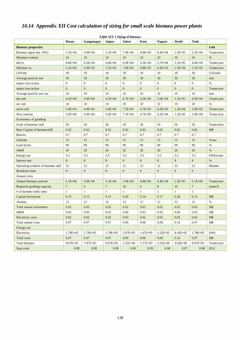
138

10.14 Appendix XII Cost calculation of sizing for small scale biomass power plants

Table XIV 1 Sizing of biomass



Biomass input (mc 10%) 5.1E+04 5.0E+04 5.1E+04 7.6E+04 4.8E+04 6.4E+04 1.3E+05 5.1E+04 Tonne/year

Moisture content 10 10 10 10 10 10 10 10 %

dm in 4.6E+04 4.5E+04 4.6E+04 6.9E+04 4.3E+04 5.7E+04 1.1E+05 4.6E+04 Tonne/year

Moisture in 5.1E+03 5.0E+03 5.1E+03 7.6E+03 4.8E+03 6.4E+03 1.3E+04 5.1E+03 Tonne/year

LHVdry 18 18 18 18 18 18 18 18 GJ/tonne

Average particle size 30 30 30 30 30 30 30 30 mm



Average particle size out 10 10 10 10 10 10 10 10 mm


mc end 10 10 10 10 10 10 10 10 %

moist end 5.0E+03 4.9E+03 5.0E+03 7.5E+03 4.7E+03 6.2E+03 1.2E+04 5.0E+03 Tonne/year


Economics of grinding

Scale of hammer mill 50 50 50 50 50 50 50 50 Tonne/hour

Base Capital of hammermill 0.62 0.62 0.62 0.62 0.62 0.62 0.62 0.62 M$

Rfactor 0.7 0.7 0.7 0.7 0.7 0.7 0.7 0.7

Lifetime 15 15 15 15 15 15 15 15 Years

Load factor 90 90 90 90 90 90 90 90 %

O&M 20 20 20 20 20 20 20 20 %

Energy use 3.5 3.5 3.5 3.5 3.5 3.5 3.5 3.5 kWh/tonne

Interest rate 8 8 8 8 8 8 8 8 %

Operating window of hammer mill 12 12 12 12 12 12 12 12 Months

Residence time 0 0 0 0 0 0 0 0

Annual costs


Required grinding capacity 7 6 7 10 6 8 16 7 tonne/h

# of hammer mills units 1 1 1 1 1 1 1 1


Annuity 12 12 12 12 12 12 12 12 %


O&M 0.03 0.03 0.03 0.04 0.03 0.03 0.06 0.03 M$



Energy use

Electricity 1.78E+05 1.74E+05 1.78E+05 2.67E+05 1.67E+05 2.22E+05 4.45E+05 1.78E+05 kWh

Total costs 0.07 0.07 0.07 0.09 0.06 0.08 0.14 0.07 M$

Total biomass 8.07E+05 7.87E+05 8.07E+05 1.21E+06 7.57E+05 1.01E+06 2.02E+06 8.07E+05 Tonne/year

Step costs 0.08 0.08 0.08 0.08 0.09 0.08 0.07 0.08 $/GJ

139

10.15 Appendix XII Cost calculation of pelletizing for small scale biomass power plants

Table XV 1 Pelletizing of biomass



Biomass input (mc 10%) 4.98E+04 4.86E+04 4.98E+04 7.48E+04 4.67E+04 6.23E+04 1.25E+05 4.98E+04 Tonne/year

Moisture content 10 10 10 10 10 10 10 10 %

Moisture in 4983 4859 4983 7475 4672 6229 12459 4983 Tonne/year

dm in 4.49E+04 4.37E+04 4.49E+04 6.73E+04 4.20E+04 5.61E+04 1.12E+05 4.49E+04 Tonne/year

LHVdry (odt) 18 18 18 18 18 18 18 18 GJ/tonne



Average particle size out 10 10 10 10 10 10 10 10 mm

Product characteristics

Form Pellets Pellets Pellets Pellets Pellets Pellets Pellets Pellets

Bulk density 650 650 650 650 650 650 650 650 kg/m3bulk

LHV (oven dry) 10 10 10 10 10 10 10 10 GJ/m3


mc end 10 10 10 10 10 10 10 10 %

moist end 4.98E+03 4.86E+03 4.98E+03 7.48E+03 4.67E+03 6.23E+03 1.25E+04 4.98E+03 Tonne/year


Economics of pelletizing

Scale of pellet mill 6 6 6 6 6 6 6 6 Tonne/hour

Base Capital of pellet mill 0.20 0.20 0.20 0.20 0.20 0.20 0.20 0.20 (M$)

Rfactor 0.61 0.61 0.61 0.61 0.61 0.61 0.61 0.61

Lifetime 10 10 10 10 10 10 10 10 Years

Load factor 90 90 90 90 90 90 90 90 %

O&M 197 197 197 197 197 197 197 197 % investment costs

Energy use 28 28 28 28 28 28 28 28 kWhe/tonne

Interest rate 8 8 8 8 8 8 8 8 %

Operating window 12 12 12 12 12 12 12 12 Months

Residence time 0 0 0 0 0 0 0 0 Months

Annual costs


Required pelletising capacity 6.4 6.2 6.4 9.6 6.0 8.0 16.0 6.4 Tonne/hour

pellet mills units 2.0 2.0 2.0 2.0 2.0 2.0 3.0 2.0


Annuity 15 15 15 15 15 15 15 15 %


O&M 0.54 0.53 0.54 0.69 0.52 0.62 1.11 0.54 M$



Energy use

Electricity 1.40E+06 1.36E+06 1.40E+06 2.09E+06 1.31E+06 1.74E+06 3.49E+06 1.40E+06 kWh

Electricity 5.02E+06 4.90E+06 5.02E+06 7.54E+06 4.71E+06 6.28E+06 1.26E+07 5.02E+06 GJ

Total costs 0.74 0.73 0.74 0.99 0.71 0.87 1.60 0.74 M$/year

Total biomass 8.07E+05 7.87E+05 8.07E+05 1.21E+06 7.57E+05 1.01E+06 2.02E+06 8.07E+05 GJ

Step costs 0.92 0.93 0.92 0.82 0.94 0.86 0.79 0.92 $/GJ

140

10.16 Appendix XVI Distance between district headquarters and power plants

Table XVI 1 2nd

transportation distance thermal power plants

Chhabra thermal power plant

Baran

Suratgarh thermal power plant

Ganganagar

Kalisindh thermal power plant

Jhalawar

Kota thermal power plant

Kota

Ajmer - 416 - -

Bhilwara - 543 214 152

Jalore - - - -

Jhalawar 116 - 13 -

Kota 152 - 84 6

Table XVI 2 2

nd transportation distance biomass based power plants

Baran Ganganagar Jaipur Jalore Nagaur Kota Sirohi Tonk

Ajmer - 506 - 76

Alwar - - 81 -

Baran - - - -

Bhilwara - - - -

Jaipur - - - -

Jalore - - - -

Jhalawar - - - -

Kota 136 - - -

Nagaur - - - -

Sirohi - - - -

Tonk - - - -

141

10.17 Appendix XIII State-wise road length and road density

Table XVII 1 Road length and road density of India

STATES Area (km2) Surfaced (km) Total (km) % Density (km/km

2)

Andhra Pradesh 275069 155579 238001 7% 0.87

Aruachal Pradesh 83743 14336 21555 1% 0.26

Assam 78550 37816 241789 8% 3.08

Bihar 94163 57198 130642 4% 1.39

Chhattisgarh 136034 64078 93965 2% 0.69

Goa 3702 7531 10627 0% 2.87

Gujarat 196024 141565 156188 5% 0.80

Haryana 44212 37701 41729 1% 0.94

Himachal Pradesh 55673 33247 47963 1% 0.86

Jammu & Kashmir 222236 14178 26980 1% 0.12

Jharkhand 79714 16379 23903 1% 0.30

Karnataka 191791 179099 281773 8% 1.47

Kerala 38863 110359 201220 7% 5.18

Madhya Pradesh 308144 119921 197293 6% 0.64

Maharashtra 307713 339794 410521 7% 1.33

Manipur 22327 8140 19133 1% 0.86

Meghalaya 22429 7072 11984 0% 0.53

Mizoram 21081 7001 9810 0% 0.47

Nagaland 16579 15470 34146 1% 2.06

Orissa 155707 58719 258836 7% 1.66

Punjab 50362 76612 84193 2% 1.67

Rajasthan 342240 194979 241318 6% 0.71

Sikkim 7096 4119 4630 0% 0.65

Tamil Nadu 130058 158473 192339 6% 1.48

Tripura 10492.69 14203 33772 1% 3.22

Uttaranchal 240928 297674 390256 1% 1.62

Uttar Pradesh 53484 26664 49277 9% 0.92

West Bengal 88752 115534 299209 7% 3.37

Source: (MOSPI. 2013)

142

10.18 Appendix XIV Village connectivity

Table XVIII 1 District-wise village connectivity

Population Group 1000 &

Above

Population Group 500 –

1000

Population Group 250 –

500

Population Group Below –

250

DISTRICT Total

Villages Connectivity %

Total


Total


Total


Ajmer 454 100 295 100 183 63 93 38

Alwar 928 100 584 100 296 39 146 29

Bansawara 437 100 425 100 324 92 196 54

Baran 243 100 342 92 286 30 218 16

Barmer 516 100 840 95 469 87 108 35

Bharatpur 627 100 391 97 214 39 134 31

Bhilwara 481 100 524 100 440 38 248 21

Bikaner 410 100 175 100 112 96 107 34

Bundi 237 100 314 96 208 34 80 18

Chittaurgarh 283 100 435 100 431 35 403 22

Churu 477 100 219 100 90 98 68 56

Dausa 396 100 299 99 165 38 165 15

Dholpur 290 99 307 93 140 33 49 39

Dungarpur 351 100 265 100 157 99 81 46

Ganganagar 318 100 465 100 676 72 1371 50

Hanumangarh 354 100 199 99 190 81 1030 38

Jaipur 850 100 649 100 356 53 222 24

Jaisalmer 136 100 174 98 134 93 156 24

Jalore 477 100 143 100 47 96 30 33

Jhalawar 262 100 448 98 465 34 302 23

Jhunjhunun 494 100 246 100 96 89 19 42

Jodhpur 635 100 273 99 107 94 43 37

Karauli 379 99 197 96 102 37 77 21

Kota 212 100 264 98 214 45 122 24

Nagaur 836 100 385 100 173 96 86 45

Pali 478 100 270 100 126 97 62 24

Pratapgarh 213 99 212 97 244 85 236 16

Rajsamand 288 100 288 100 260 54 137 23

Sawai Madhopur 311 99 199 94 122 37 87 29

Sikar 635 100 226 100 73 96 52 42

Sirohi 233 100 124 99 46 61 52 21

Tonk 290 98 278 97 260 28 204 21

Udaipur 667 100 603 97 507 75 400 27

TOTAL 14198 100 11058 98 7713 60 6784 33

Source: (Gov of Raj. 2013d)

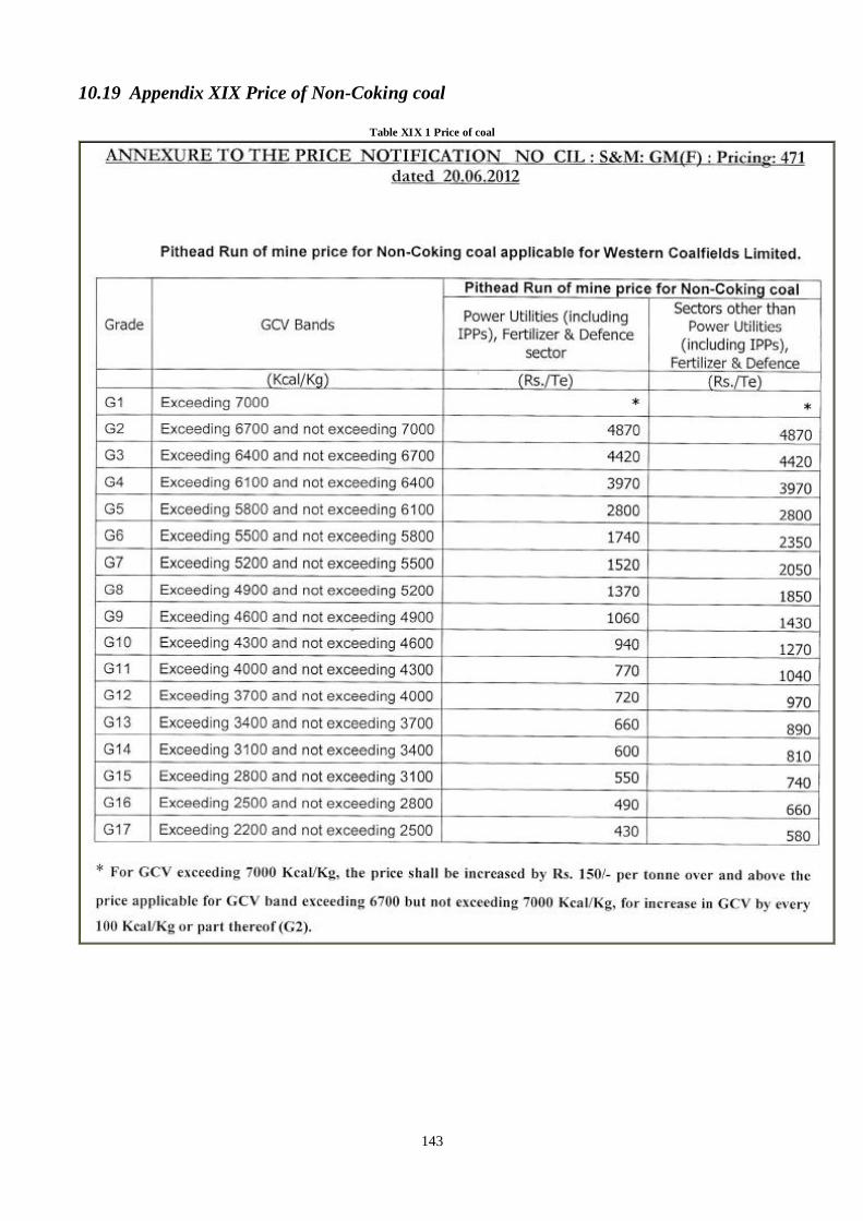
143

10.19 Appendix XIX Price of Non-Coking coal

Table XIX 1 Price of coal

144

10.20 Appendix XX Railway freight rate and goods classification Table XX 1 Railway freight rate per tonne

Table XX 2 Classification of goods

145

10.21 Appendix XXI Estimated cost of selected supply chains biomass power plants from

districts with the lowest cost of supply

Figure XXI 1 Cost of selected supply chains for Jaipur from Ajmer

Figure XXI 2 Cost of selected supply chains Jalore from Jalore

Figure XXI 3 Cost of selected supply chains Kota from Kota

146

Figure XXI 4 Cost of selected supply chains for Nagaur from

Figure XXI 5 Cost of selected supply chains for Tonk from Tonk

147

10.22 Appendix XXII District-wise estimated cost of selected supply chains biomass based

power plants Table XXII 1 Cost of production at the power plant gate Baran district ($/GJ)

District Logs Chips Pellets District Logs Chips Pellets

Ajmer 5.4 5.9 5.9 Jaipur 7.2 7.6 7.7

Alwar 6.6 7.1 7.0 Jaisalmer 20.3 21.1 20.5

Barmer 16.9 17.7 17.3 Jalore 7.4 8.0 7.5


Baran 4.1 5.0 5.9 Jhunjhunu 8.1 8.7 8.3



Bikaner 14.4 15.1 14.8 Kota 4.3 4.6 5.2

Bundi 5.0 5.3 5.9 Nagaur 13.0 13.5 13.5


Churu 11.4 12.0 11.7 Rajsamand 6.0 6.5 6.4

Dausa 6.4 6.8 7.0 Sikar 7.8 8.4 8.1

Dholpur 7.7 8.1 8.3 Sirohi 7.4 8.0 7.6


Ganganagar 14.5 15.4 14.5 Tonk 5.5 5.9 6.1


Table XXII 2 Cost of production at the power plant gate Ganganagar district ($/GJ)

District Logs Chips Pellets District Logs Chips Pellets

Ajmer 6.7 7.2 6.9 Jaipur 7.8 8.4 8.2

Alwar 6.9 7.4 7.1 Jaisalmer 18.6 19.2 19.1

Barmer 16.6 17.3 17.0 Jalore 8.0 8.7 8.0


Baran 10.3 11.1 10.1 Jhunjhunu 6.5 6.9 7.0



Bikaner 11.7 12.0 12.6 Kota 8.6 9.3 8.5

Bundi 8.7 9.4 8.7 Nagaur 12.0 12.4 12.7


Churu 9.1 9.5 9.9 Rajsamand 8.3 9.1 8.2

Dausa 8.0 8.6 8.2 Sikar 6.8 7.2 7.3

Dholpur 10.0 10.7 10.1 Sirohi 8.9 9.7 8.7


Ganganagar 7.9 9.0 10.0 Tonk 7.8 8.5 7.9


148

Table XXII 3 Cost of production at the power plant gate Jaipur district ($/GJ)

District Logs Chips Chips (dry) Pellets District Logs Chips Chips (dry) Pellets

Ajmer 4.7 5.0 5.3 Jaipur 3.9 5.0 5.1 5.1 6.1

Alwar 4.0 4.1 4.9 Jaisalmer 18.9 19.6 19.4 18.1 19.4

Barmer 16.6 17.3 17.0 Jalore 7.5 8.1 7.6 5.2 6.2

Banswara 8.5 9.2 8.6 Jhalawar 7.1 7.6 7.5 5.4 6.5

Baran 7.6 8.1 8.0 Jhunjhunu 4.9 5.1 5.8 5.1 6.1

Bharatpur 5.6 5.9 6.4 Jodhpur 8.3 8.8 8.7 7.0 8.0

Bhilwara 5.7 6.1 6.2 Karauli 4.9 5.2 5.6 4.3 5.3

Bikaner 12.4 12.8 13.2 Kota 6.0 6.4 6.5 4.6 5.7

Bundi 6.1 6.5 6.7 Nagaur 11.5 11.9 12.3 11.2 12.4

Chittaurgarh 6.7 7.2 7.1 Pali 6.1 6.6 6.5 4.6 5.7

Churu 8.3 8.6 9.3 Rajsamand 6.4 6.9 6.7 4.7 5.7

Dausa 5.1 5.3 5.9 Sikar 5.1 5.3 6.0 5.0 6.1

Dholpur 7.1 7.5 7.8 Sirohi 7.4 8.0 7.5 5.4 6.5

Dungarpur 8.4 9.1 8.5 Sawai madhopur 5.3 5.6 6.0 4.5 5.5

Ganganagar 11.4 11.9 12.0 Tonk 5.2 5.5 5.8 4.3 5.4

Hanumangarh 11.8 12.2 12.6 Udaipur 8.4 9.0 8.7 6.6 7.7

Table XXII 4 Cost of production at the power plant gate Jalore district ($/GJ)

District Logs Chips Chips (Dry) Pellets District Logs Chips Chips (Dry) Pellets

Ajmer 6.0 6.4 6.3 Jaipur 8.5 9.0 8.6 6.4 7.3

Alwar 8.6 9.2 8.4 Jaisalmer 16.5 16.8 17.5 17.1 18.2

Barmer 12.9 13.0 14.0 Jalore 2.8 2.9 3.8 3.8 4.8


Baran 9.2 9.8 9.2 Jhunjhunu 8.8 9.4 8.7 6.5 7.4



Bikaner 13.6 14.0 14.0 Kota 7.5 8.0 7.5 5.7 6.6

Bundi 7.8 8.4 7.9 Nagaur 12.3 12.7 12.9 11.2 12.3


Churu 11.7 12.3 11.8 Rajsamand 5.4 5.7 5.8 4.0 4.9

Dausa 8.7 9.3 8.6 Sikar 8.5 9.0 8.5 6.4 7.3

Dholpur 11.0 11.8 10.7 Sirohi 4.5 4.7 5.2 3.9 4.9


Ganganagar 13.9 14.6 13.8 Tonk 7.5 8.1 7.6 4.5 5.5


149

Table XXII 5 Cost of production at the power plant gate Kota district ($/GJ)

District Logs Chips (Wet) Chips (Dry) Pellets District Logs Chips (Wet) Chips (Dry) Pellets

Ajmer 4.5 4.4 5.2 Jaipur 6.3 6.1 6.9 5.8 6.9

Alwar 5.9 5.9 6.4 Jaisalmer 19.3 19.6 19.8 18.5 19.8

Barmer 16.0 16.2 16.5 Jalore 6.8 6.9 7.1 5.7 6.7


Baran 5.1 4.8 6.1 Jhunjhunu 7.2 7.2 7.6 6.1 7.1



Bikaner 13.5 13.6 14.0 Kota 2.9 3.0 4.0 3.8 4.9

Bundi 4.1 3.8 5.1 Nagaur 12.0 12.0 12.7 11.6 12.7


Churu 10.4 10.5 10.9 Rajsamand 5.0 4.9 5.6 4.4 5.4

Dausa 5.7 5.6 6.4 Sikar 6.2 6.1 6.8 6.0 7.1

Dholpur 7.7 7.6 8.2 Sirohi 6.5 6.5 6.8 5.9 6.9


Ganganagar 13.6 13.9 13.7 Tonk 4.6 4.4 5.4 4.3 5.4


Table XXII 6 Cost of production at the power plant gate Nagaur district ($/GJ)


Ajmer 3.5 3.6 4.3 Jaipur 5.9 6.2 6.6 5.9 6.9

Alwar 6.0 6.4 6.4 Jaisalmer 17.2 17.7 18.0 17.0 18.2

Barmer 14.2 14.6 15.1 Jalore 5.6 6.0 6.1 4.7 5.7


Baran 7.4 7.8 7.8 Jhunjhunu 6.0 6.3 6.6 5.4 6.3



Bikaner 11.3 11.6 12.3 Kota 5.7 6.1 6.1 5.1 6.0

Bundi 5.8 6.2 6.4 Nagaur 8.8 8.9 10.2 10.4 11.5


Churu 9.0 9.4 9.8 Rajsamand 4.8 5.1 5.4 3.8 4.8

Dausa 6.1 6.5 6.7 Sikar 5.7 6.0 6.4 6.1 7.1

Dholpur 8.4 9.0 8.8 Sirohi 5.4 5.8 6.0 5.0 5.9


Ganganagar 11.7 12.2 12.2 Tonk 5.0 5.3 5.6 5.0 6.0


150

Table XXII 7 Cost of production at the power plant gate Sirohi district


Ajmer 5.0 5.4 5.5 Jaipur 7.5 8.0 7.8 6.6 7.5

Alwar 7.5 8.2 7.6 Jaisalmer 17.0 17.5 17.9 17.1 18.2

Barmer 13.4 13.7 14.4 Jalore 3.8 4.0 4.6 3.8 4.7


Baran 8.1 8.6 8.3 Jhunjhunu 8.1 8.7 8.2 6.4 7.3



Bikaner 13.1 13.6 13.7 Kota 6.3 6.8 6.6 5.8 6.6

Bundi 6.7 7.2 7.0 Nagaur 11.7 12.1 12.4 11.4 12.4


Churu 11.2 11.8 11.4 Rajsamand 4.2 4.4 4.9 3.8 4.7

Dausa 7.7 8.2 7.8 Sikar 7.8 8.3 8.0 6.3 7.2

Dholpur 10.0 10.7 10.0 Sirohi 2.9 3.0 4.0 3.8 4.7


Ganganagar 13.7 14.5 13.7 Tonk 6.5 7.0 6.8 5.2 6.1


Table XXII 8 Cost of production at the power plant gate Tonk district ($/GJ)


Ajmer 4.3 4.6 5.1 Jaipur 5.4 5.6 6.2 5.5 6.5

Alwar 5.2 5.5 5.8 Jaisalmer 19.3 20.0 19.7 18.3 19.5

Barmer 16.2 16.9 16.7 Jalore 7.3 7.9 7.4 4.5 5.5


Baran 5.7 5.9 6.5 Jhunjhunu 6.3 6.7 6.9 5.1 6.1



Bikaner 13.3 13.9 13.9 Kota 4.2 4.4 5.1 4.2 5.3

Bundi 4.4 4.6 5.3 Nagaur 11.9 12.3 12.6 11.5 12.6


Churu 9.5 10.0 10.2 Rajsamand 5.3 5.7 5.9 4.7 5.7

Dausa 5.0 5.2 5.9 Sikar 6.0 6.3 6.7 5.4 6.5

Dholpur 6.9 7.3 7.6 Sirohi 6.9 7.5 7.2 5.2 6.3


Ganganagar 12.8 13.4 13.1 Tonk 2.9 3.0 4.1 3.9 5.0


151

10.23 Appendix XXIII Cost of electricity production biomass based power plants

Figure XXIII 1 Biomass power plant Jaipur

Figure XXIII 2 Biomass power plant Jalore

Figure XXIII 3 Biomass power plant Kota

152

Figure XXIII 4 Biomass power plant Nagaur

Figure XXIII 5 Biomass power plant Tonk

153

10.24 Appendix XXIV Sensitivity analysis discount rate, labour wages and yield

Figure XXIV 1 Sensitivity analysis discount rate



154


Figure XXIV 5 Sensitivity analysis labour wages


155



Figure XXIV 9 Sensitivity analysis yield